Spin-Orbital Ordering in Alkali Superoxides

Abstract

Akali superoxides $A$O2 ($A=\textrm{Na}$, K, Rb, Cs), due to an open $p$ shell of the oxygen ion O2^- with degenerate $\pi$ orbitals, have spin and orbital degrees of freedom. The complex magnetic, orbital, and structural phase transitions observed experimentally in this family of materials are only partially understood. Based on density functional theory, we derive a strong-coupling effective model for the isostructural compounds $A$O2 ($A=\textrm{K}$, Rb, Cs) from a two-orbital Hubbard model. We find that CsO2 has highly frustrated exchange interactions in the $a$-$b$ plane, while the frustration is weaker for smaller alkali ions. We solve the resulting Kugel-Khomskii model in the mean-field approximation. We show that CsO2 exhibits an antiferro-orbital (AFO) order with the ordering vector $\bm{q}=(1,0,0)$ and a stripe antiferromagnetic order with $\bm{q}=(1/2,0,0)$, which is consistent with recent neutron scattering experiments. We discuss the role of the $\pi$-orbital degrees of freedom for the experimentally observed magnetic transitions and interpret the as-yet-unidentified $T_{\mathrm{s2}}=70$ K transition in CsO2 as an orbital ordering transition.

I Introduction

O2 is a unique molecule that possesses a magnetic moment $S=1$ on its own. Solid oxygen, in which O2 molecules are aggregated by the van der Waals force, exhibits a variety of electronic properties such as antiferromagnetism, metal-to-insulator transition [1], and superconductivity [2] under temperature and pressure variations.

Another interesting system composed of O2 molecules is an ionic crystal, where O2 molecules act as electron acceptors for the counter metal ions. Alkali superoxides $A$O2 ($A=\textrm{Na}$, K, Rb, Cs) are famous examples of such compounds [3]. The O2^- ion has three electrons in the anti-bonding $\pi_{g}^{\ast}$ orbitals, which consist of two orbital states with symmetries similar to $d_{zx}$ and $d_{yz}$. Hence, one hole per O2^- molecule having spin $S=1/2$ and orbital degrees of freedom dominate the low-temperature physical properties. As a consequence, spin and orbital physics as in $d$ electron systems are expected.

Electronically, alkali superoxides exhibit insulating behavior for all temperatures. Since the unit cell contains an odd number of electrons, the insulating behavior is ascribed to the Coulomb repulsion. A first-principles assessment with dynamical mean-field theory for RbO2 concluded that RbO2 is indeed a Mott insulator [4]. This indicates that $A$O2 ($A=\textrm{K}$, Rb, Cs) are strongly correlated electron systems consisting of $\pi$ electrons.

Three compounds KO2, RbO2, and CsO2 with the exception of NaO2 take the same crystal structure at room temperature [5, 6, 7, 8, 9]. The temperature variation of crystal structure and magnetic properties is summarized in Fig. 1. Above 400 K, $A$O2 exhibits the cubic NaCl-type ($Fm\bar{3}m$, no. 225) crystal structure, in which O2 molecules are disoriented (phase I). At around room temperature, the O2 molecules are oriented parallel to the $c$ axis (phase II), and the crystal structure of $A$O2 becomes tetragonal ($I4/mmm$, no. 139) with $a=b<c$. Figure 2 (a) shows the crystal structure in phase II. Phases below 200 K are material dependent, although there is a tendency that a smaller alkali radius leads to a lower symmetry. KO2 undergoes two steps of symmetry lowering to monoclinic at $T=196$ K and to triclinic at $T\simeq 10$ K [7]. RbO2 first loses the four-fold symmetry to become orthorhombic ($Immm$, no. 71) with $a\neq b$ at $T=194$ K and is slightly distorted to $\gamma=90.6^{\circ}$ (angle between $a$ and $b$ axes) to become monoclinic below $T=90$ K [9, 10]. CsO2 undergoes only one structural transition from tetragonal to orthorhombic ($Immm$) at $T=T_{\mathrm{s1}}\simeq 150$ K [7, 11].

Figure 1: Summary of the structural phase transitions and magnetic properties in CsO2, RbO2, and KO2. [5, 7, 8, 9]

Magnetic properties of KO2 and RbO2 follow the Curie-Weiss law. A transition to the antiferromagnetic (AFM) state has been observed at $T_{\mathrm{N}}\simeq 10$ K and $T_{\mathrm{N}}\simeq 15$ K, respectively [8]. The magnetic structure of KO2 has been identified to be AFM with ordering vector $\bm{q}=(1,0,0)$ in units of the reciprocal lattice vector of the conventional unit cell [12]. For RbO2, the magnetic structure has not been determined, although full magnetic volume fraction has been confirmed [10]. On the other hand, CsO2 shows peculiar magnetic properties. The susceptibility $\chi(T)$ in CsO2 follows the Curie-Weiss law down to $T=T_{\mathrm{s2}}\simeq 70$ K [13, 11]. Below $T_{\mathrm{s2}}$, $\chi(T)$ takes a maximum and is suppressed as $T$ decreases. This indicates a development of short-range spin correlations. It is reported that $\chi(T)$ in this region is well fitted by the Bonner-Fisher function, which was taken to suggest that the magnetic properties are described by the one-dimensional antiferromagnetic Heisenberg model [13, 11]. At $T=T_{\mathrm{N}}=9.6$ K, an AFM transition takes place [8]. Recent neutron scattering experiments revealed a stripe-type magnetic structure [14, 15]. Two experiments proposed different propagation vectors $\bm{q}=(0,1/2,0)$ [14] and $\bm{q}=(1/2,0,0)$ [15], in the orthorhombic structure with $a<b$.

These experimental results demonstrate the diverse structural and magnetic properties in $A$O2 ($A=\textrm{K}$, Rb, Cs). For a comprehensive understanding, the following two issues need to be addressed: (i) What is the relevant microscopic control parameter that governs the physical properties in $A$O2? An apparent parameter that systematically changes for different $A$ atoms is the lattice parameter, which increases in the order of K, Rb, and Cs. However, it is highly nontrivial why the short-range correlations are clearly observed only in CsO2, which has the largest O2–O2 distance. We thus raise a more specific issue: (ii) What is the electronic state of CsO2? The role of the orbitals in the magnetic properties is of particular interest.

Theoretical studies have addressed the electronic structure in RbO2 [16, 17, 18, 4] and KO2 [19, 20, 21, 22, 23]. Regarding the correlated magnetic behavior in CsO2, Riyadi et al. proposed a zigzag orbital ordered state [13]. By assuming only hopping between O2-$\pi_{g}^{*}$ and Cs-$5p$, they argue that super-exchange interaction is allowed only on a one-dimensional zigzag path in the $a$-$b$ plane. The magnetic properties have been investigated by NMR [24], electron paramagnetic resonance [25], and high-field magnetization measurement [11].

In this paper, we derive an effective spin-orbital model for $A$O2 based on first-principles calculations. We will demonstrate that geometrical frustration is the key element that constitutes a difference between $A$ atoms: The frustration plays a crucial role in CsO2 but is less important in KO2 and RbO2. With a mean-field calculation, we will propose an alternative type of orbital order in CsO2 that leads to the magnetic state with the experimentally observed stripe AFM order.

The rest of this paper is organized as follows. We first derive the electronic structure of $A$O2 and an approximate tight-binding model in Sec. II. Using perturbation theory, we derive an effective model describing intersite spin and orbital interactions in Sec. III. Possible spin and orbital phase transitions are identified using the mean-field (MF) approximation in Sec. IV. Based on these results, we discuss implications for $A$O2 in Sec. V. Results are summarized in Sec. VI.

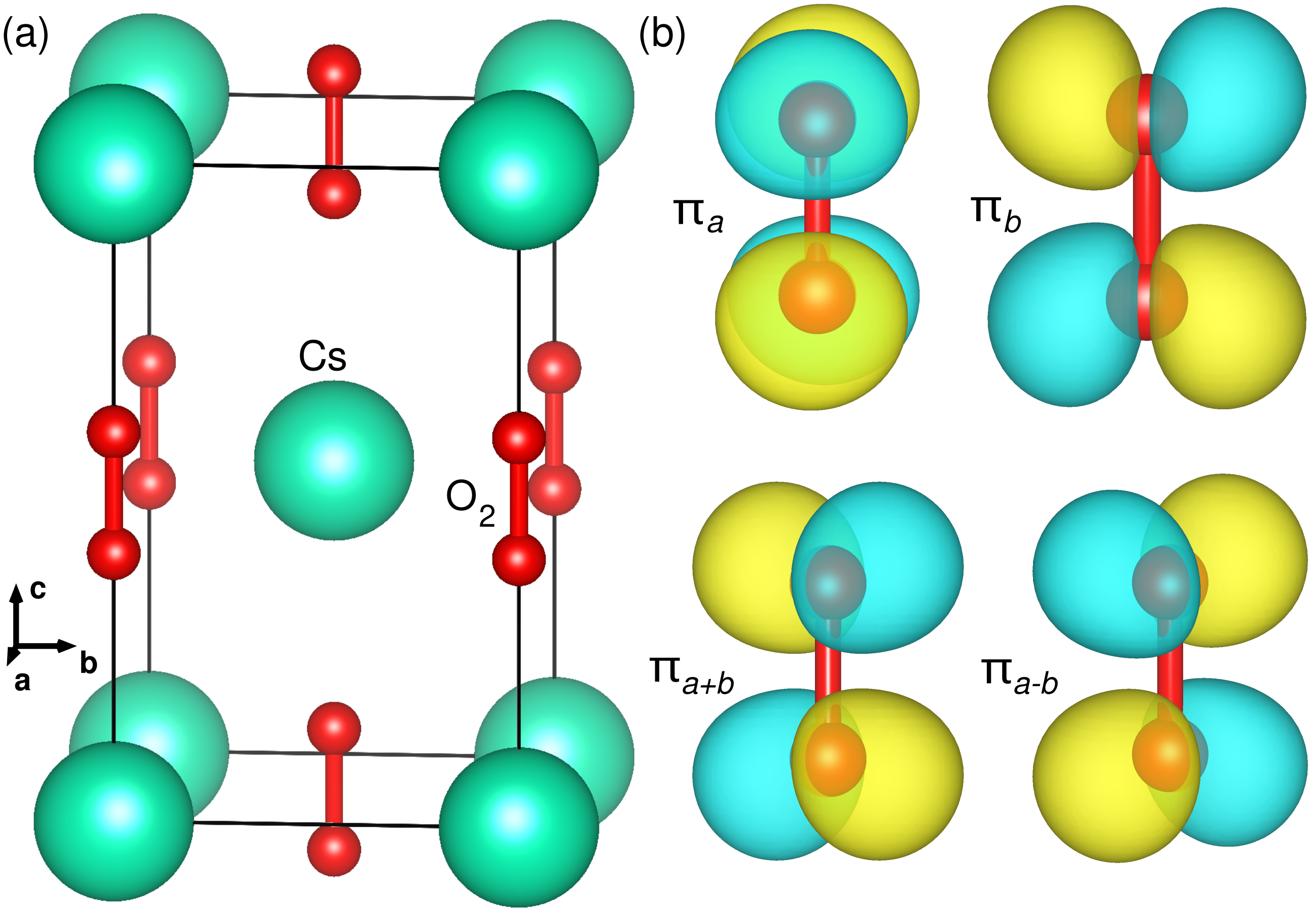
Figure 2: (a) Structure of tetragonal CsO2 ($I4/mmm$ space group). (b) Wannier functions of oxygen $\pi_{g}^{*}$ orbitals in $(\pi_{a}$, $\pi_{b})$ basis and in $(\pi_{a+b}$, $\pi_{a-b})$ basis.

Table 1: Crystal structures used in the density functional theory calculations. O $z$ positions in brackets are obtained by structure optimization within GGA.

material	SG	$T$ [K]	$a$ [Å]	$b$ [Å]	$c$ [Å]	O $z$	Ref.
CsO2	$Immm$	40	4.37164	4.40176	7.34214	0.412030 (0.408076)	9
CsO2	$I4/mmm$	300	4.46529	$=a$	7.32980	0.422770 (0.407922)	9
RbO2	$Immm$	130	4.14325	4.16334	7.00745	0.40656 (0.403463)	9
RbO2	$I4/mmm$	300	4.20866	$=a$	7.00572	0.407160 (0.403441)	9
KO2	$I4/mmm$	298	4.03334	$=a$	6.69900	0.40450 (0.399067)	26

II Electronic structure

We perform our density functional theory calculations using the all electron full potential local orbital (FPLO) basis set [27]. We use the generalized gradient approximation exchange correlation functional [28]. In order to extract suitable tight-binding models, we employ the symmetry preserving projective Wannier functions of FPLO [29]. We base our calculation on the structures specified in Table 1.

Figure 3 (a) shows the band structure and density of states of the room-temperature structure of CsO2 ($I4/mmm$ space group). The $\bm{k}$-path is a standard one for the body-centered tetragonal structure [30, 31]. There are only two $\pi_{g}^{\star}$ orbitals of oxygen near the Fermi level. The weights of the two $\pi_{g}^{\ast}$ Wannier functions are shown in Figure 3 (b). The weights are not equally distributed in the path segments $Y-\Gamma$ and $Z-P$ along which either only $k_{x}$ or only $k_{y}$ changes. The dispersion of the two $\pi_{g}^{\star}$ bands of RbO2 and KO2 at room temperature ($I4/mmm$ structure) is very similar to CsO2.

Figure 4 shows the results for the $T=40$ K structure of CsO2 ($Immm$ space group). At $\Gamma$, the $\pi_{b}$ band is 14 meV below the $\pi_{a}$ band because the $b$ axis is 0.7% longer than the $a$ axis. RbO2 in $Immm$ space group ($T=130$ K structure) exhibits a similar dispersion of $\pi_{g}^{\star}$ orbitals near the Fermi level.

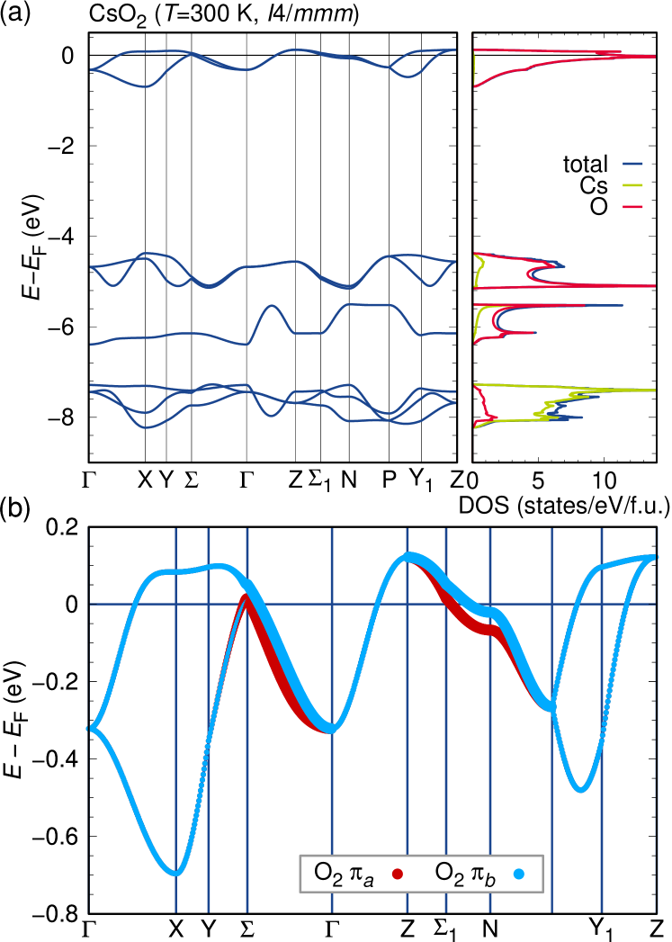
Figure 3: (a) Band structure and density of states of CsO2 in $I4/mmm$ space group ($T=300$ K structure). The $\bm{k}$-points are defined in [31]. (b) Wannier fit of the two bands near $E_{\rm F}$ with weights of the $\pi_{a}$ and $\pi_{b}$ Wannier orbitals.

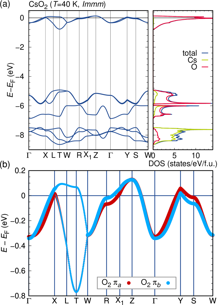
Figure 4: (a) Band structure and density of states of CsO2 in $Immm$ space group ($T=40$ K structure). The $\bm{k}$-points are defined in [32]. (b) Wannier fit of the two bands near $E_{\rm F}$ with weights of the $\pi_{a}$ and $\pi_{b}$ Wannier orbitals.

The band structure near the Fermi level can be well described by a two-orbital tight-binding model consisting of the two $\pi_{g}^{*}$ orbitals. Figure 2 (b) shows Wannier orbitals of the $\pi_{g}^{*}$ in two sets of representations. The ($\pi_{a}$, $\pi_{b}$) basis describes orbitals that extend along $a$ and $b$ axes, while ($\pi_{a+b}$, $\pi_{a-b}$) basis describes orbitals that extend to the $[110]$ and $[1\bar{1}0]$ directions. These representations are converted to each other by

$$\begin{pmatrix}\ket{\pi_{a-b}}\\ \ket{\pi_{a+b}}\end{pmatrix}=\frac{1}{\sqrt{2}}\begin{pmatrix}1&-1\\ 1&1\end{pmatrix}\begin{pmatrix}\ket{\pi_{a}}\\ \ket{\pi_{b}}\end{pmatrix}.$$ (1)

Figure 5 shows three kinds of dominant bonds, which include the hopping along the $a$ or $b$ axis (denoted by $l=a$, $b$), the diagonal hopping in the $a$-$b$ plane ($l=a+b$), and the hopping between the corner site and the body-center site ($l=\textrm{BC}$). The hopping matrix $t_{ij}^{\gamma\gamma^{\prime}}$ becomes diagonal in the ($\pi_{a}$, $\pi_{b}$) basis for $l=a$ and $b$, and diagonal in the ($\pi_{a+b}$, $\pi_{a-b}$) basis for $l=a+b$ and BC. We assign two eigenvalues to $\pi$ and $\delta$ hopping following the usual convention [33], and represent them by $t_{\pi}^{l}$ and $t_{\delta}^{l}$, respectively. The hopping parameters computed using DFT and projective Wannier functions are summarized in Table 2. The tight binding bands computed only with the hoppings along three paths in the tetragonal case and along four paths in the orthorhombic case perfectly reproduce the original dispersion in Figs. 3 and 4.

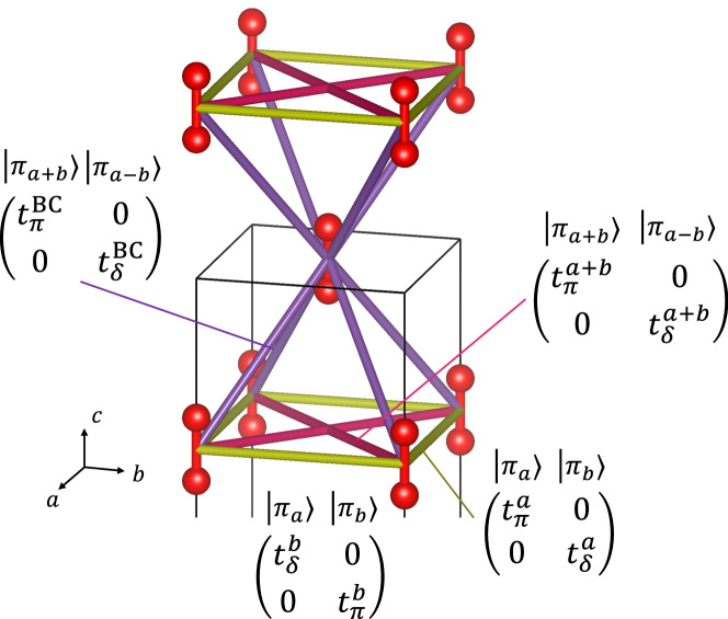
Figure 5: Relevant transfer integrals between $\pi_{g}^{\ast}$ orbitals on the O2^- ions.

Table 2: The hopping parameters, $t_{\pi}^{l}$ and $t_{\delta}^{l}$, for $A$O2 in units of meV. Other quantities, $t$, $\theta$, $\phi$, and $r^{l}$, are defined from $t_{\pi}^{l}$ and $t_{\delta}^{l}$. See Eqs. (2)–(4) for the definitions. “opt O $z$” means the use of the optimized O $z$ positions (the values in the brackets in Table 1).

	material	SG		$t^{a}_{\pi}$	$t^{a}_{\delta}$	$t^{b}_{\pi}$	$t^{b}_{\delta}$	$t^{a+b}_{\pi}$	$t^{a+b}_{\delta}$	$t^{\mathrm{BC}}_{\pi}$	$t^{\mathrm{BC}}_{\delta}$	$t$	$\theta$	$\phi$	$r^{ab}$	$r^{a+b}$	$r^{\mathrm{BC}}$
(i)	CsO2	$Immm$		39	23	36	24	-38	-2	-82	22	84	$16.6^{\circ}$	$45.8^{\circ}$	0.63	0.05	-0.27
(ii)	CsO2	$Immm$	(opt O $z$)	36	22	33	23	-34	0	-80	21	81	$14.5^{\circ}$	$43.6^{\circ}$	0.66	0.01	-0.26
(iii)	CsO2	$I4/mmm$		55	27	55	27	-43	-1	-102	30	105	$18.8^{\circ}$	$31.4^{\circ}$	0.49	0.02	-0.29
(iv)	CsO2	$I4/mmm$	(opt O $z$)	32	19	32	19	-28	0	-78	20	79	$12.0^{\circ}$	$37.4^{\circ}$	0.59	0	-0.26
(v)	RbO2	$Immm$		55	15	53	15	-28	0	-94	26	97	$18.9^{\circ}$	$15.0^{\circ}$	0.27	0	-0.29
(vi)	RbO2	$Immm$	(opt O $z$)	52	14	50	14	-26	0	-92	25	95	$17.7^{\circ}$	$14.6^{\circ}$	0.28	0.02	-0.27
(vii)	RbO2	$I4/mmm$		52	13	52	13	-25	-1	-92	26	94	$18.2^{\circ}$	$13.0^{\circ}$	0.25	0.04	-0.28
(viii)	RbO2	$I4/mmm$	(opt O $z$)	48	12	48	12	-23	0	-90	25	92	$16.6^{\circ}$	$12.8^{\circ}$	0.25	0.02	-0.27
	KO2	$I4/mmm$		68	6	68	6	-19	-1	-109	31	113	$21.3^{\circ}$	$4.5^{\circ}$	0.09	0.05	-0.28
	KO2	$I4/mmm$	(opt O $z$)	63	5	63	5	-17	0	-107	30	110	$19.3^{\circ}$	$4.1^{\circ}$	0.08	0.02	-0.23

In order to characterize differences in the hopping parameters between the three compounds, we introduce two kinds of dimensionless parameters as follows. Firstly, the ratio between $t_{\pi}^{l}$ and $t_{\delta}^{l}$ for each bond $l$ is defined as $r^{l}\equiv t_{\delta}^{l}/t_{\pi}^{l}$. Table 2 indicates that $|r^{l}|$ ranges from 0 to 0.68 depending on the bond and $A$ atoms. Here, we averaged $r^{a}$ and $r^{b}$ as $r^{ab}\equiv(r^{a}+r^{b})/2$. Secondly, the relation between different bonds is represented by three-dimensional polar coordinates defined by

$$(t_{\pi}^{\textrm{BC}})^{2} =t^{2}\cos\theta,$$ (2)

$$(t_{\pi}^{\textrm{ab}})^{2} =t^{2}\sin\theta\cos\phi,$$ (3)

$$(t_{\pi}^{\textrm{a}+\textrm{b}})^{2} =t^{2}\sin\theta\sin\phi,$$ (4)

where $(t_{\pi}^{\textrm{ab}})^{2}\equiv[(t_{\pi}^{\textrm{a}})^{2}+(t_{\pi}^{\textrm{b}})^{2}]/2$. Here, we consider the square of the hopping parameters because the effective intersite exchange interactions are proportional to $t^{2}$ rather than $t$ itself (Sec. III). A graphical interpretation of $\theta$ and $\phi$ is presented in Fig. 6. The north pole corresponds to a system with only the nearest-neighbor hopping $t^{\mathrm{BC}}$, while the equator corresponds to a two-dimensional square lattice model with $t^{a}$ and $t^{a+b}$. Combinations of two or more hopping parameters lead to geometrical frustration of the exchange interactions. In particular, $\phi=45^{\circ}$ leads to a two-dimensional frustration within the $a$-$b$ plane, while $\theta=45^{\circ}$ leads to a three-dimensional frustration between $l=\mathrm{BC}$ bond and in-plane bonds.

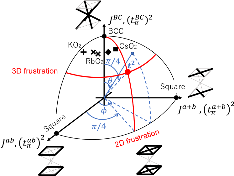
Figure 6: Parameterization of the bond-dependence of the transfer integrals using polar coordinates. The symbols indicate the DFT estimates for CsO2, RbO2, and KO2 (only results without the optimization are shown).

DFT estimates of $\theta$ and $\phi$ are presented in Table 2 and marked with symbols in Fig. 6. The $A$O2 series is located in the $\theta<45^{\circ}$ region, which means that the $l=\mathrm{BC}$ bond is the largest and three-dimensional hopping plays a major role. Regarding the hopping in the $a$-$b$ plane, CsO2 is located around $\phi=45^{\circ}$, which indicates that CsO2 is characterized by two-dimensional frustration between $l=a$ and $a+b$ bonds. This frustration is largest in CsO2 and tends to get weaker for smaller alkali ions.

III Strong-coupling effective model

Since $A$O2 ($A=\textrm{K}$, Rb, Cs) are Mott insulators [4], we employ a strong-coupling effective model that describes intersite exchange interactions between localized spin and orbital degrees of freedom. We first compare two kinds of exchange interactions, and then derive an explicit form of the Hamiltonian.

III.1 Comparison between kinetic exchange and superexchange interactions

There are two perturbation processes that give rise to intersite exchange interactions between $\pi_{g}^{*}$ electrons on the O2^- ions. One is the second-order process of the O2^—O2^- hopping (kinetic exchange), and the other is the fourth-order process of the O2^—Cs^+ hopping (super-exchange). The coupling constant of the kinetic exchange interaction, $J_{\mathrm{kinetic}}$, is estimated to be

$$J_{\mathrm{kinetic}}\sim\frac{t^{2}}{U},$$ (5)

where $U$ is the Coulomb repulsion between two electrons on the same orbital. On the other hand, the coupling constant of the super-exchange interaction through Cs^+ ions, $J_{\mathrm{super}}$, is estimated to be

$$J_{\mathrm{super}}\sim\frac{(t_{\textrm{Cs-O}_{2}})^{4}}{U\Delta_{5p}^{2}},$$ (6)

where $t_{\textrm{Cs-O}_{2}}$ is the hopping amplitude between the O2-$\pi_{g}^{*}$ orbital and the Cs-$5p$ orbital. We estimated $t_{\textrm{Cs-O}_{2}}$ by projecting the energy dispersion in Fig. 4 onto an eight-band tight-binding model consisting of O2-$\pi_{g}^{*}$, $\pi_{u}$, $\sigma_{g}$, and Cs-$5p$ orbitals. We thus concluded that $t_{\textrm{Cs-O}_{2}}$ is the same order as $t$ in the two-band model, namely, $t\sim t_{\textrm{Cs-O}_{2}}$. Hence, the ratio between $J_{\mathrm{kinetic}}$ and $J_{\mathrm{super}}$ is estimated as

$$\frac{J_{\mathrm{super}}}{J_{\mathrm{kinetic}}}\sim\frac{t^{2}}{\Delta_{5p}^{2}}\sim 10^{-4}.$$ (7)

Here, we used $t\sim 0.1$ eV (Table 2) and $\Delta_{5p}\sim 8$ eV (Fig. 4). Therefore, we consider from now on only the kinetic exchange interaction by the direct O2–O2 hopping, neglecting the superexchange process through Cs.

III.2 Derivation of the interactions

In order to derive the kinetic exchange interactions, we begin with the two-orbital Hubbard model consisting of the $\pi_{g}^{*}$ orbitals, $\pi_{a}$ and $\pi_{b}$. The Hamiltonian reads

$$H= \sum_{\langle ij\rangle}\sum_{\gamma\gamma^{\prime}\sigma}t^{\gamma\gamma^{\prime}}_{ij}(c^{{\dagger}}_{i\gamma\sigma}c_{j\gamma^{\prime}\sigma}+\textrm{h.c.})+U\sum_{i\gamma}n_{i\gamma\uparrow}n_{i\gamma\downarrow}$$

$$+U^{\prime}\sum_{i\gamma>\gamma^{\prime}}n_{i\gamma}n_{i\gamma^{\prime}}+J_{\mathrm{H}}\sum_{i\sigma\sigma^{\prime}\gamma>\gamma^{\prime}}c^{{\dagger}}_{i\gamma\sigma}c^{{\dagger}}_{i\gamma^{\prime}\sigma^{\prime}}c_{i\gamma\sigma^{\prime}}c_{i\gamma^{\prime}\sigma}$$

$$+J^{\prime}_{\mathrm{H}}\sum_{i\gamma\neq\gamma^{\prime}}c^{{\dagger}}_{i\gamma\uparrow}c^{{\dagger}}_{i\gamma\downarrow}c_{i\gamma^{\prime}\downarrow}c_{i\gamma^{\prime}\uparrow},$$ (8)

where $c_{i\gamma\sigma}$ is the annihilation operator for site $i$, orbital $\gamma$, and spin $\sigma$, and $n_{i\gamma\sigma}=c^{{\dagger}}_{i\gamma\sigma}c_{i\gamma\sigma}$ is the number operator. The first term represents the electron hopping between site $i$ and site $j$. The symbol $\langle ij\rangle$ stands for the pairs of neighboring O2 sites shown in Fig. 5. The second and third terms represent the intra-orbital and inter-orbital Coulomb repulsion, respectively. The fourth and fifth terms represent the Hund’s rule coupling and the pair hopping interaction, respectively.

We consider the Mott insulating state with the occupation number $n=3$ per site. For convenience, we treat this as $n=1$ from now on, using a hole picture. Note that the relation between orbital states and lattice distortion is reversed in the hole picture, though the effective Hamiltonian derived below is the same for $n=1$ and $n=3$. The local electronic degrees of freedom in the Mott insulating state are described by the spin and orbital (pseudo-spin) operators defined by

$$\bm{S}_{i}=\frac{1}{2}\sum_{\gamma\sigma\sigma^{\prime}}c_{i\gamma\sigma}^{{\dagger}}\bm{\sigma}_{\sigma\sigma^{\prime}}c_{i\gamma\sigma^{\prime}},$$ (9)

$$\bm{T}_{i}=\frac{1}{2}\sum_{\gamma\gamma^{\prime}\sigma}c_{i\gamma\sigma}^{{\dagger}}\bm{\sigma}_{\gamma\gamma^{\prime}}c_{i\gamma^{\prime}\sigma},$$ (10)

where $\bm{\sigma}=(\sigma^{x},\sigma^{y},\sigma^{z})$ is the Pauli matrix. The eigenstates of $T^{z}$ are $\ket{\pi_{a}}$ and $\ket{\pi_{b}}$ orbitals, which extend along the $a$ and $b$ axes, respectively [Fig. 2 (b)]. On the other hand, the eigenstates of $T^{x}$ describe $\ket{\pi_{a+b}}$ and $\ket{\pi_{a-b}}$ orbitals that extend to the diagonal direction [Fig. 2 (b)], because the ($\pi_{a+b}$, $\pi_{a-b}$) basis is obtained by linear combination of ($\pi_{a}$, $\pi_{b}$) as given in Eq. (1). In general, we can describe the orbital state in an arbitrary direction by rotating $T^{z}$ and $T^{x}$ in the pseudo-spin space as

$$\widetilde{T}^{z}(\varphi) =T^{z}\cos\varphi+T^{x}\sin\varphi,$$

$$\widetilde{T}^{x}(\varphi) =-T^{z}\sin\varphi+T^{x}\cos\varphi.$$ (11)

Figure 7 shows the variation of the eigenstates of the operators $\widetilde{T}^{z}$ and $\widetilde{T}^{x}$. The orbital state is rotated by $\varphi/2$ around the $c$ axis.

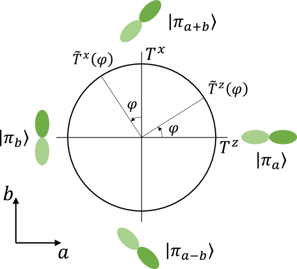
Figure 7: A diagram for the orbital (pseudo-spin) operators and the orbital states. The orbital on the right (left) represents the eigenstate of the operator $T^{z}$ with the eigenvalue $+1/2$ ($-1/2$). The orbital state is rotated around the $c$ axis by $\varphi/2$ as the operator is rotated by $\varphi$ in the pseudo-spin space.

In second-order perturbation theory around the atomic limit with respect to the hopping, the effective Hamiltonian $\mathcal{H}_{\mathrm{eff}}$ for the $n=1$ subspace is given by

$$\mathcal{H}_{\mathrm{eff}}= -2\sum_{\langle ij\rangle}J_{1}^{l}\left(\frac{3}{4}+\bm{S}_{i}\cdot\bm{S}_{j}\right)\left\{\left[1+\left(r^{l}\right)^{2}\right]\left(\frac{1}{4}-\tau_{i}^{l}\tau_{j}^{l}\right)-r^{l}\left(\tau_{i}^{l+}\tau_{j}^{l-}+\tau_{i}^{l-}\tau_{j}^{l+}\right)\right\}$$

$$-2\sum_{\langle ij\rangle}J_{2}^{l}\left(\frac{1}{4}-\bm{S}_{i}\cdot\bm{S}_{j}\right)\left\{\left[1+\left(r^{l}\right)^{2}\right]\left(\frac{1}{4}-\tau_{i}^{l}\tau_{j}^{l}\right)+r^{l}\left(\tau_{i}^{l+}\tau_{j}^{l-}+\tau_{i}^{l-}\tau_{j}^{l+}\right)\right\}$$

$$-2\sum_{\langle ij\rangle}J_{2}^{{}^{\prime}l}\left(\frac{1}{4}-\bm{S}_{i}\cdot\bm{S}_{j}\right)\left[\left(\frac{1}{2}+\tau_{i}^{l}\right)\left(\frac{1}{2}+\tau_{j}^{l}\right)+\left(r^{l}\right)^{2}\left(\frac{1}{2}-\tau_{i}^{l}\right)\left(\frac{1}{2}-\tau_{j}^{l}\right)-r^{l}\left(\tau_{i}^{l+}\tau_{j}^{l+}+\tau_{i}^{l-}\tau_{j}^{l-}\right)\right]$$

$$-2\sum_{\langle ij\rangle}J_{3}^{l}\left(\frac{1}{4}-\bm{S}_{i}\cdot\bm{S}_{j}\right)\left[\left(\frac{1}{2}+\tau_{i}^{l}\right)\left(\frac{1}{2}+\tau_{j}^{l}\right)+\left(r^{l}\right)^{2}\left(\frac{1}{2}-\tau_{i}^{l}\right)\left(\frac{1}{2}-\tau_{j}^{l}\right)+r^{l}\left(\tau_{i}^{l+}\tau_{j}^{l+}+\tau_{i}^{l-}\tau_{j}^{l-}\right)\right],$$ (12)

where $l$ is the bond index that takes the values $a$, $b$, $a+b$, $a-b$, BC, or $\overline{\textrm{BC}}$, depending on the combination of $i$ and $j$ (Fig. 8). Here, we introduced $l=a-b$ and $\overline{\textrm{BC}}$, which have the same hopping parameter as $l=a+b$ and BC, respectively, but are different in the definition of the operator $\tau_{i}^{l}$ (see below). The coupling constants $J_{1}^{l},J_{2}^{l},J_{2}^{{}^{\prime}l}$, and $J_{3}^{l}$ are given by

$$J_{1}^{l} =\frac{(t_{\pi}^{l})^{2}}{U^{{}^{\prime}}-J_{\mathrm{H}}},$$

$$J_{2}^{l} =\frac{(t_{\pi}^{l})^{2}}{U^{{}^{\prime}}+J_{\mathrm{H}}},$$

$${J_{2}^{{}^{\prime}}}^{l} =\frac{(t_{\pi}^{l})^{2}}{U-J_{\mathrm{H}}^{{}^{\prime}}},$$

$$J_{3}^{l} =\frac{(t_{\pi}^{l})^{2}}{U+J_{\mathrm{H}}^{{}^{\prime}}}.$$ (13)

The operators $\tau^{l}$ and $\tau^{l\pm}$ are bond-dependent orbital operators defined by

$$\tau^{l} =\widetilde{T}^{z}(2\varphi_{l}),$$

$$\tau^{l\pm} =\widetilde{T}^{x}(2\varphi_{l})\pm iT^{y},$$ (14)

where $\varphi_{l}$ is the azimuthal angle around the $c$ axis: $\varphi_{a}=0$, $\varphi_{a+b}=\varphi_{\mathrm{BC}}=\pi/4$, $\varphi_{b}=\pi/2$, and $\varphi_{a-b}=\varphi_{\mathrm{\overline{BC}}}=3\pi/4$. The coupling constants satisfy $J_{1}^{l}>J_{2}^{l}\simeq J_{2}^{{}^{\prime}l}>J_{3}^{l}$ in a typical choice of parameters. Details are given in Appendix A.

Equation (12) includes $\delta$ hopping, which is expressed by the coefficient $r^{l}\equiv t_{\delta}^{l}/t_{\pi}^{l}$. Without $r^{l}$ terms, namely, inserting $r^{l}=0$ into Eq. (12), $\mathcal{H}_{\mathrm{eff}}$ is reduced to the well-known form of the Kugel-Khomskii (KK) Hamiltonian for $d$-$e_{g}$ orbital systems [34, 35, 36, 37, 38]. We note that the definition of the bond-dependent orbital operator $\tau^{l}$ in Eq. (14) is different from that in $e_{g}$ orbital systems, since the rotation of the $\pi_{g}^{*}$ orbitals follows the rule in Eq. (1), which is different from that for $e_{g}$ orbitals. The KK-type interaction for $\pi$ electron systems has also been derived in the context of organic conductors [39, 40] and RbO2 [17, 18].

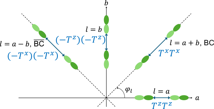
Figure 8: The orbital-orbital interactions, $\tau_{i}^{l}\tau_{j}^{l}$, described by the bond-dependent orbital operator $\tau_{i}^{l}$.

Figure 8 shows examples of the bond-dependent orbital interactions in Eq. (12). For the $l=a$ bond, $\tau^{l}$ is given by $\tau^{l}=T^{z}$ and hence the ($\pi_{a}$, $\pi_{b}$) basis is relevant. Depending on the sign of the coefficient for $T^{z}_{i}T^{z}_{j}$, either $\pi_{a}$ or $\pi_{b}$ is uniformly aligned [ferro-orbital (FO) order] or $\pi_{a}$ and $\pi_{b}$ orbitals are alternately aligned [antiferro-orbital (AFO) order]. The $l=b$ bond has the same interaction $T^{z}_{i}T^{z}_{j}$, since $\tau^{l}=-T^{z}$. The difference between $l=a$ and $l=b$ arises in the operator $(1/2+\tau_{i}^{l})$, which projects onto the $\pi_{a}$ ($\pi_{b}$) orbital for $l=a$ ($l=b$). On the other hand, the interaction is described by the $\tau^{l}=T^{x}$ ($-T^{x}$) operator for $l=a+b$ and $l=\textrm{BC}$ ($l=a-b$ and $l=\overline{\textrm{BC}}$). Therefore, if the interactions of the diagonal in the $a$-$b$ plane or the body-center are dominant, the orbital tends to form $\pi_{a+b}$ or $\pi_{a-b}$ orbitals.

IV Mean-field calculations

IV.1 Calculation details

We apply the mean-field (MF) approximation to search for possible phase transitions emerging in the effective model in Eq. (12). The order parameters include $\expectationvalue*{T_{i}^{\xi}}$, $\expectationvalue{S_{i}^{z}}$, and $\expectationvalue*{S_{i}^{z}T_{i}^{\xi}}$, where $\xi=x,y,z$ and $\expectationvalue{\cdot}$ stands for the thermal average. We set $\expectationvalue{S_{i}^{x}}=\expectationvalue{S_{i}^{y}}=\expectationvalue*{S_{i}^{x}T_{i}^{\xi}}=\expectationvalue*{S_{i}^{y}T_{i}^{\xi}}=0$ to enforce the spin moment along the $S^{z}$ direction, because the spin orientation is arbitrary in the present model without spin-orbit coupling.

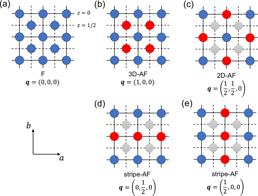
Figure 9: Configurations of the ordered states. The ordering vector $\bm{q}$ is indicated in units of the reciprocal lattice vectors of the conventional unit cell. The circles with the same color represent the same spin or orbital state. The gray sites are not involved in the two-dimensional ordered states in (c)–(e). The sites connected by the solid (dashed) lines represent the layer at $z=0$ ($z=1/2$), respectively. States are labeled F for ferro-orbital/ferromagnetic and AF for antiferro-orbital/antiferromagnetic.

We consider 8 sublattices in a $2\times 2\times 2$ supercell. Five possible configurations are shown in Fig. 9. There are (a) one ferroic (F) and (b)–(e) four antiferroic (AF) configurations. (b) 3D-AF is the three-dimensional AF configuration with the ordering vector $\bm{q}=(1,0,0)$ [which may also be expressed as $\bm{q}=(0,1,0)$ or $\bm{q}=(0,0,1)$]. The rest are two-dimensional AF configurations: (c) 2D-AF is the AF order on the square lattice with the ordering vector $\bm{q}=(1/2,1/2,0)$. (d) and (e) are stripe-AF with the ordering vector $\bm{q}=(0,1/2,0)$ and $\bm{q}=(1/2,0,0)$, respectively. They are degenerate in a tetragonal model. For reference, various ordered states in the Heisenberg model on the bcc lattice are discussed in Ref. [41].

The spin and orbital separately take one of the five configurations in Fig. 9. We address spin (orbital) configurations by adding M (O) at the end of the configuration name (here, M stands for magnetic or magnetism). Examples include 3D-AFM and stripe-AFO order.

We define the Fourier components of the order parameters as $\expectationvalue*{T^{\xi}_{\bm{q}}}=(1/N)\sum_{i}\expectationvalue*{T^{\xi}_{i}}e^{-i\bm{q}\cdot\bm{R}_{i}}$, where $\bm{R}_{i}$ is the coordinate of site $i$ and $N$ is the number of sites. We use a simplified notation by replacing $\bm{q}$ with the name of the configuration in Fig. 9. For example, $\expectationvalue*{T^{\xi}}_{\textrm{3D-AF}}$ stands for $\expectationvalue*{T^{\xi}_{\bm{q}}}$ with $\bm{q}=(1,0,0)$ and $\expectationvalue*{S^{z}}_{\textrm{stripe-AF}}$ stands for $\expectationvalue*{S^{z}_{\bm{q}}}$ with $\bm{q}=(1/2,0,0)$ or $(0,1/2,0)$.

There are four interaction parameters, $U$, $U^{\prime}$, $J_{\mathrm{H}}$, and $J_{\mathrm{H}}^{\prime}$. We use the standard relations $U^{\prime}=U-2J_{\mathrm{H}}$ and $J_{\mathrm{H}}^{\prime}=J_{\mathrm{H}}$ that are valid in $e_{g}$ orbital systems. Once the ratio $J_{\mathrm{H}}/U$ is given, the effective Hamiltonian $\mathcal{H}_{\mathrm{eff}}$ in Eq. (12) is proportional to $J\equiv t^{2}/U$. Hence, we vary $J_{\mathrm{H}}/U$, and measure the temperature $T$ in units of $J$. As a reference, the values of $U$ and $J_{\mathrm{H}}$ were estimated for KO2 using a constrained DFT scheme [19], which gives $U\approx 3.55$ eV and $J_{\mathrm{H}}\approx 0.62$ eV, and thus $J_{\mathrm{H}}/U\approx 0.17$. Another estimate on solid oxygen yields $U\approx 11.6$ eV $J_{\rm H}\approx 0.82$ eV, and thus $J_{\rm H}/U\approx 0.07$, by the van-der-Waals density functional plus $U$ method [42] and optical absorption experiment [43]. From these estimates, we fix the ratio as $J_{\rm H}/U=0.1$ in the following calculations, unless otherwise noted.

Regarding the hopping term, there are three parameters $\theta$, $\phi$, and $r^{l}$. We fix $r^{l}$ to the value for CsO2 [(iv) in Table 2] and vary $\theta$ and $\phi$ to get a comprehensive understanding of the present model. This will highlight the importance of the geometrical frustration in CsO2 compared to KO2 and RbO2. Then, we focus on CsO2 and RbO2 and discuss the influence of the distortion in the low-temperature phase in Sec. IV.3.

IV.2 Ground-state phase diagram for the tetragonal structure

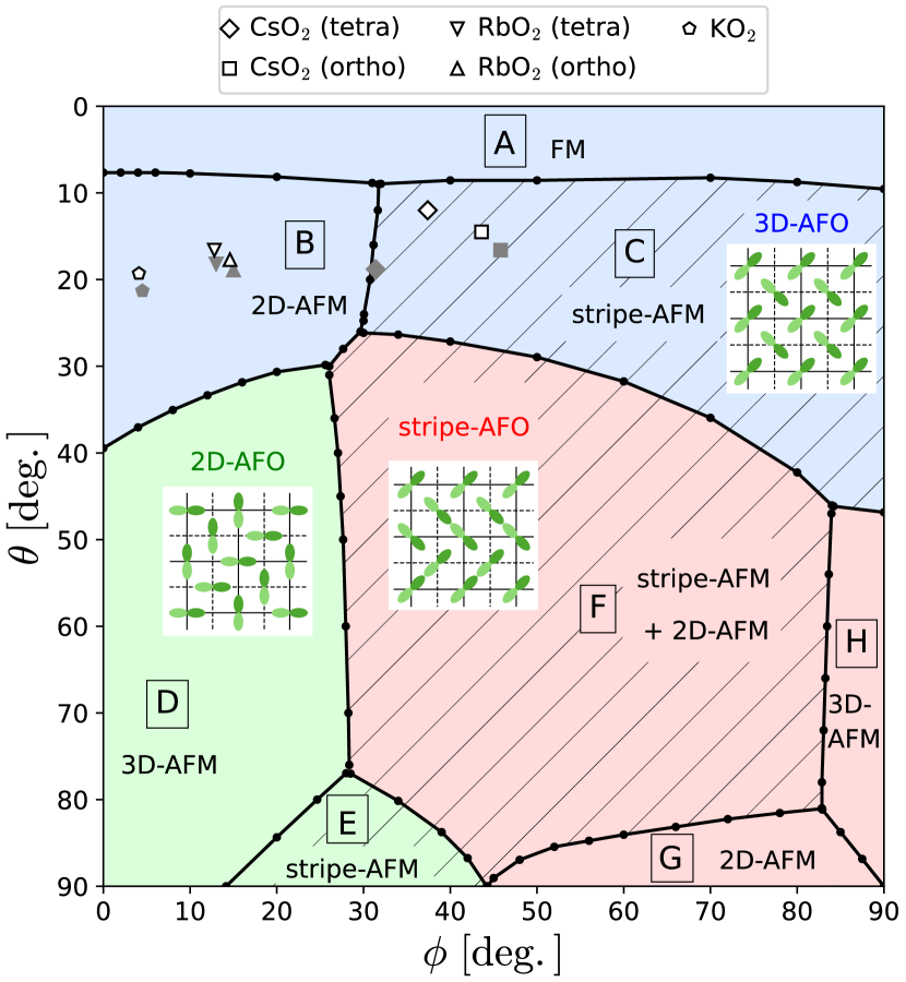
Figure 10: The ground-state phase diagram of the tetragonal model in the $(\phi,\theta)$ plane for $J_{\mathrm{H}}/U=0.10$. The background colors distinguish orbital states. The diagonally shaded areas indicate phases having stripe-AFM order. The symbols indicate the DFT estimates for CsO2, RbO2, and KO2 (see Table 2). The open symbols are for the optimized O $z$ positions, and the filled symbols are for the experimental values. The spin-orbital configuration of each phase is shown in Fig. 11. The values of $r^{l}$ were set to (iv) in Table 2.

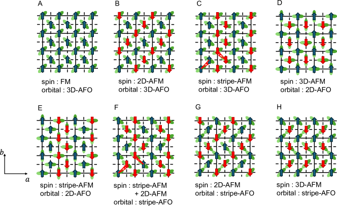
Figure 11: Schematic diagrams of the spin-orbital ordered states appearing in the phase diagram for the tetragonal model in Fig. 10, The arrows represent spins. The stripe-AF orders have two degenerate states with $\bm{q}=(1/2,0,0)$ and $\bm{q}=(0,1/2,0)$. The one stabilized under orthorhombic distortion with $a<b$ is shown.

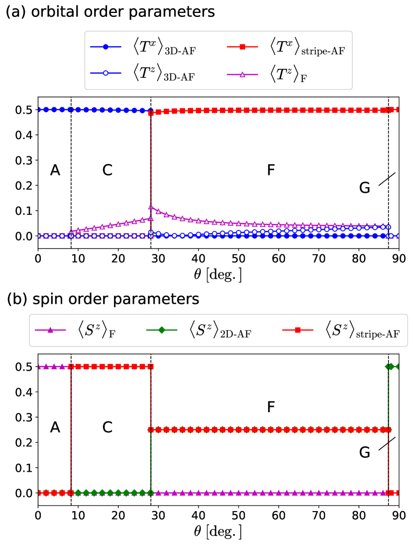
Figure 12: (a) The orbital and (b) spin order parameters in the ground state as functions of $\theta$ for $\phi=46^{\circ}$ and $J_{\mathrm{H}}/U=0.1$. The labels such as $\expectationvalue{S^{z}}_{\textrm{F}}$ and $\expectationvalue{T^{x}}_{\textrm{3D-AF}}$ stand for the Fourier components, where the subscript indicates the configuration in Fig. 9. A, C , F, and G represent the labels of spin-orbital ordered phases listed in Fig. 11. The hopping parameters are set to (iv) in Table 2.

The ground-state phase diagram in the $\phi$-$\theta$ plane is shown in Fig. 10, where the values of $r^{ab}$, $r^{a+b}$, and $r^{\rm BC}$ are fixed to the parameter set (iv) in Table 2. The blue, green, and red regions represent the orbital ordered phases with the propagation vectors $\bm{q}=(1,0,0)$ (3D-AFO order), $\bm{q}=(1/2,1/2,0)$ (2D-AFO order), and $\bm{q}=(0,1/2,0)$ or $(1/2,0,0)$ (stripe-AFO order), respectively. The diagonally hatched area corresponds to the stripe-AFM phases, and the other areas are the FM, 2D-AFM, or 3D-AFM ordered phases.

There are eight kinds of ordered phases, termed A-H as shown in Fig. 11, by the combinations of the spin order and orbital patterns and the ordered components of the orbital moment. The overall trend is that the 3D-AFO ordered phases are stabilized in the small $\theta$ region ($\theta<40^{\circ}$), while in the large-$\theta$ region, the 2D-AFO and stripe-AFO ordered phases compete with each other and a phase transition occurs around $\phi=30$–$40^{\circ}$. This is because small $\theta$ means that $(t_{\pi}^{\textrm{BC}})^{2}$ dominates over $(t_{\pi}^{\textrm{ab}})^{2}$ and $(t_{\pi}^{\textrm{a}+\textrm{b}})^{2}$, and the opposite is true for large $\theta$. The phase competition between these three orbital ordered states is reproduced by the MF approximation on the orbital-only model obtained by setting the spin operators in Eq. (12) to zero, presented in Appendix B. Since the change of the spin configurations strongly depends on the underlying orbital order patterns as well as on $\phi$ and $\theta$, the details will be described in the following.

Here, let us investigate changes of order parameters as a function of $\theta$ while fixing $\phi=46^{\circ}$, corresponding to the hopping parameters of tetragonal CsO₂. Figure 12 (a) shows the Fourier components of the orbital order parameters, $\expectationvalue{T^{x}}_{\textrm{3D-AF}}$, $\expectationvalue{T^{x}}_{\textrm{stripe-AF}}$, and $\expectationvalue{T^{z}}_{\textrm{F}}$; $\expectationvalue{T^{x}}_{\textrm{3D-AF}}$ and $\expectationvalue{T^{x}}_{\textrm{stripe-AF}}$ represent staggered alignments of $\pi_{a+b}$ and $\pi_{a-b}$ orbitals along the $c$ axis and the $a$ or $b$ axis, respectively, and $\expectationvalue{T^{z}}_{\textrm{F}}$ denotes the uniform order of $\pi_{a}$ or $\pi_{b}$ orbital. In Fig. 12 (b), the spin order parameters, $\expectationvalue{S^{z}}_{\textrm{F}}$, $\expectationvalue{S^{z}}_{\textrm{stripe-AF}}$, and $\expectationvalue{S^{z}}_{\textrm{2D-AF}}$ are plotted, which characterize the FM, stripe-AFM, and 2D-AFM order of the $S^{z}$ component, respectively. All the order parameters are defined so that their maximum values are $0.5$.

At $\theta=0$, $\expectationvalue{T^{x}}_{\textrm{3D-AF}}$ and $\expectationvalue{S^{z}}_{\textrm{F}}$ take the value $0.5$, showing that the phase A (FM + 3D-AFO order) shown in Fig. 11 is realized. When $\theta$ increases, $\expectationvalue{T^{x}}_{\textrm{3D-AF}}$ slightly decreases from $0.5$ and instead $\expectationvalue{T^{z}}_{\textrm{F}}$ becomes finite and increases above $\theta\simeq 8^{\circ}$. Simultaneously, the $\expectationvalue{S^{z}}_{\textrm{F}}$ discontinuously drops to zero and $\expectationvalue{S^{z}}_{\textrm{stripe-AF}}$ jumps to the maximum value. This is a first-order phase transition from phase A to C (stripe-AFM + 3D-AFO order). We note that in phase C the direction of the $\pi$ orbital shows canting towards the $a$ axis due to the small $\expectationvalue{T^{z}}_{\textrm{F}}$ as shown in Fig. 11.

Further increasing $\theta$ in Fig. 12, the dominant orbital order parameter changes to $\expectationvalue{T^{x}}_{\textrm{stripe-AF}}$ and the canting component $\expectationvalue{T^{z}}_{\textrm{F}}$ begins to decrease for $\theta\gtrsim 28^{\circ}$. As for the spin sector, $\expectationvalue{S^{z}}_{\textrm{stripe-AF}}$ discontinuously decreases and coexists with $\expectationvalue{S^{z}}_{\textrm{2D-AF}}$. This is because the stripe-AFM and 2D-AFM orders separately develop on the $z=0$ and $1/2$ planes, respectively, as the phase F in Fig. 11. These results indicate that the ground state changes from phase C to phase F at $\theta\simeq 28^{\circ}$. When $\theta$ approaches the maximum value $90^{\circ}$, only two of the constituents in phase F, $\expectationvalue{T^{x}}_{\textrm{stripe-AF}}$ and $\expectationvalue{S^{z}}_{\textrm{2D-AF}}$, remain finite and the canting of the orbitals vanishes (phase G).

For $\phi\lesssim 44^{\circ}$ in the phase diagram in Fig. 10, phases B, D, and E (see Fig. 11) appear in the region with $\theta>10^{\circ}$. Phase B has the same orbital configuration (3D-AFO order of $T^{x}$) with phase A, while the spin pattern is 2D-AFM. Increasing $\theta$ from phase B, the system enters phase D, where the orbital and spin configurations change to the 2D-AFO order of $T^{z}$ and 3F-AFM order, respectively. In phase E, which is stabilized for $\theta\gtrsim 80^{\circ}$, the orbital configuration is the same as in the neighboring phase D whereas the spin configuration is stripe-AFM, which is common to the other neighboring phase F. On the other hand, in phase H near $\phi=90^{\circ}$, the 3D-AFM order appears on the stripe-AFO order, which is shared with phases F and G.

The DFT estimates of $(\theta,\phi)$ for CsO2, RbO2, and KO2 (Table 2) are indicated by symbols in Fig. 10, showing that CsO2 is located in phase C but in the competing region with adjacent phases A, B, and F. We note that, since other parameters $r^{l}=t_{\delta}^{l}/t_{\pi}^{l}$ were fixed at the value for CsO2, the symbols of RbO2 and KO2 should be take just for reference; however, as we will show below, the full set of parameters still leads to phase B for RbO2.

IV.3 Influence of distortion

In the previous subsection, we have investigated stable spin and orbital ordered states in the tetragonal structure common to the $A$O2 at room temperature. Here, we discuss the influence of the lattice distortion which depends on each compound at low temperatures, especially focusing on the orthorhombic CsO2 and monoclinic RbO2. Since KO2 shows a triclinic structure accompanied by tilting of O₂ molecules, which is beyond our effective model assuming the O-O bond parallel to the $c$ axis, we leave it for future work.

IV.3.1 Orthorhombic distortion in CsO2

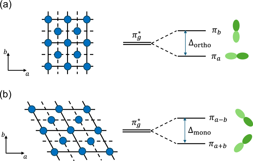
Figure 13: Schematic diagrams of (a) the orthorhombic distortion with $a<b$ and (b) the monoclinic distortion with $\gamma>90^{\circ}$, and the resultant CEF splitting of the $\pi_{g}^{\ast}$ orbitals.

CsO2 has the orthorhombic structure with $a<b$ for $T<T_{\mathrm{s1}}\simeq 150$ K (Fig. 1). The orthorhombic crystalline electric field (CEF) lifts the degeneracy between $\pi_{a}$ and $\pi_{b}$ orbitals as illustrated in Fig. 13 (a). We note that the distortion $a<b$ stabilizes the $\pi_{a}$ orbital in the hole picture. This energy splitting due to the orthorhombic distortion can be represented using the operator $T^{z}$ as

$$\mathcal{H}_{\mathrm{CEF}}=-\Delta_{\mathrm{ortho}}\sum_{i}T_{i}^{z}.$$ (15)

We thus consider the orthorhombic model given by $\widetilde{\mathcal{H}}_{\mathrm{eff}}=\mathcal{H}_{\mathrm{eff}}+\mathcal{H}_{\mathrm{CEF}}$ and adopt the parameter set (ii) in Table. 2 as the hopping parameters for the low-temperature structure of CsO₂.

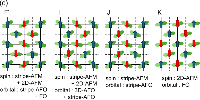
Figure 14: (a) The orbital and (b) spin order parameters in the orthorhombic model as a function of $\Delta_{\mathrm{ortho}}$ defined in Eq. (15). The hopping parameters (ii) in Table 2 were used. The arrow represents the DFT estimate for the orthorhombic CsO2, $\Delta_{\mathrm{ortho}}/(t^{2}/U)=0.60$. (c) Schematic ordering patterns in the orthorhombic model.

Figure 14 (a) and 14 (b) show the $\Delta_{\mathrm{ortho}}$ dependence of the orbital and spin order parameters, respectively. In the absence of $\Delta_{\mathrm{ortho}}$, the ground state is phase C, which is the same as in the tetragonal CsO₂ [parameter set (iv)] shown in Fig. 10. When $\Delta_{\mathrm{ortho}}$ is introduced, $\expectationvalue{T^{z}}_{\textrm{F}}$, which directly couples to the CEF, monotonically increases and the spin and orbital patterns successively change. At $\Delta_{\mathrm{ortho}}/(t^{2}/U)\simeq 0.81$, $\expectationvalue{T^{x}}_{\textrm{3D-AF}}$ discontinuously decreases, and simultaneously, other five orbital order parameters plotted in Fig. 14 (a) become finite. In the spin sector in Fig. 14 (b), $\expectationvalue{S^{z}}_{\textrm{2D-AF}}$ and $\expectationvalue{S^{z}}_{\textrm{stripe-AF}}$ are finite at the same value, indicating the coexistence of the 2D-AFM order and the stripe-AFM order as in phase F. This ordered state, termed phase I, is represented by the diagram in Fig. 14 (c). Based on the state in phase F, the orbitals are canted to the $a$ axis accompanied by the stripe-AFO order with $\bm{q}=(0,1/2,0)$ on the $z=0$ plane. When $\Delta_{\mathrm{ortho}}$ is slightly increased in phase I, the ground state changes to phase F^′, which is stable in a wide range of $\Delta_{\mathrm{ortho}}$. The orbital pattern of phase F^′ is that the $z=1/2$ plane (stripe-AFO order) in phase F is replaced by the FO order of $\pi_{a}$ orbitals. Further increasing $\Delta_{\mathrm{ortho}}$, the orbital pattern of the $z=0$ plane is also forced to FO order, and accordingly, phase K with the 2D-AFM order in all planes, shown in Fig. 14 (c), becomes stable.

According to the DFT calculation for orthorhombic CsO₂ [parameter set (ii) in Table. 2], the CEF splitting is estimated to be $\Delta_{\mathrm{ortho}}=1.1$ meV, which is normalized as $\Delta_{\mathrm{ortho}}/(t^{2}/U)\approx 0.60$, using $t=81$ meV and $U=3.55$ eV [19]. This is located in phase C as indicated by arrows in Figs. 14 (a) and 14 (b). Figure 15 shows the ground-state phase diagram obtained by changing $\phi$ and $\theta$ in the presence of the orthorhombic distortion with $\Delta_{\mathrm{ortho}}/(t^{2}/U)=0.60$. Comparing with the phase diagram for the tetragonal model in Fig. 10, we can see that, although the minor phases I and F^′ develop in the parameter region surrounded by phases A, B, C, D, and F, the overall structure of the phase diagram does not change significantly. In addition, the narrow phase J appears between phases C and H in the large $\phi$ region, where both the orbital and spin orders are stripe-AF configuration.

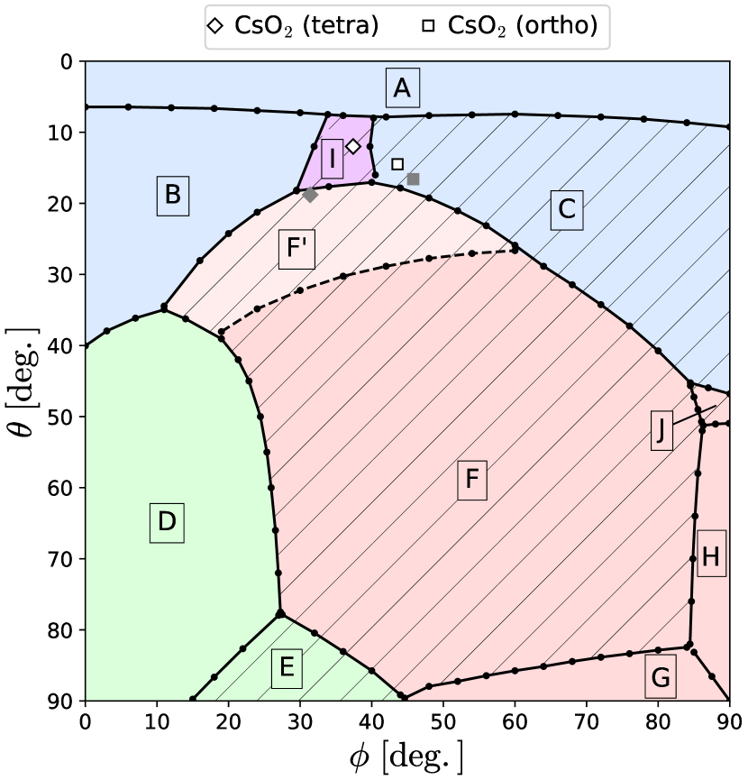
Figure 15: The ground-state phase diagram of the orthorhombic model in the $(\phi,\theta)$ plane. The symbols indicate the DFT estimates for CsO2. See the caption of Fig. 10 for more details. The parameter set (ii) in Table 2 were used with $\Delta_{\mathrm{ortho}}/(t^{2}/U)=0.60$.

IV.3.2 Monoclinic distortion in RbO2

RbO2 undergoes two structural phase transitions from tetragonal to orthorhombic, $a\neq b$, and then to monoclinic, $\gamma\neq 90^{\circ}$, with decreasing temperature, as shown in Fig. 1. The distortion of the angle with $\gamma>90^{\circ}$ lifts the degeneracy of the $\pi_{g}^{\ast}$ orbitals into $\pi_{a+b}$ and $\pi_{a-b}$ orbitals as illustrated in Fig. 13 (a). This energy splitting can be represented using the operator $T^{x}$. Hence, the CEF potential in the monoclinic phase is given by the combination of $T^{x}$ and $T^{z}$ as

$$\mathcal{H}_{\mathrm{CEF}}=-\sum_{i}(\Delta_{\mathrm{ortho}}T_{i}^{z}+\Delta_{\mathrm{mono}}T_{i}^{x}).$$ (16)

We estimated $\Delta_{\mathrm{ortho}}$ and $\Delta_{\mathrm{mono}}$ by the DFT calculation for the monoclinic structure (not shown), and obtained $\Delta_{\mathrm{ortho}}=1.15$ meV and $\Delta_{\mathrm{mono}}=4.95$ meV. We fix the ratio $\Delta_{\mathrm{ortho}}/\Delta_{\mathrm{mono}}=0.232$ and vary $\Delta_{\mathrm{mono}}$ to discuss the influence of the monoclinic CEF in RbO2. The hopping parameters $r^{l}$ for the monoclinic structure differ from those for the orthorhombic structure only by 0.01. Hence, we adopt the values in (vi) of Table 2.

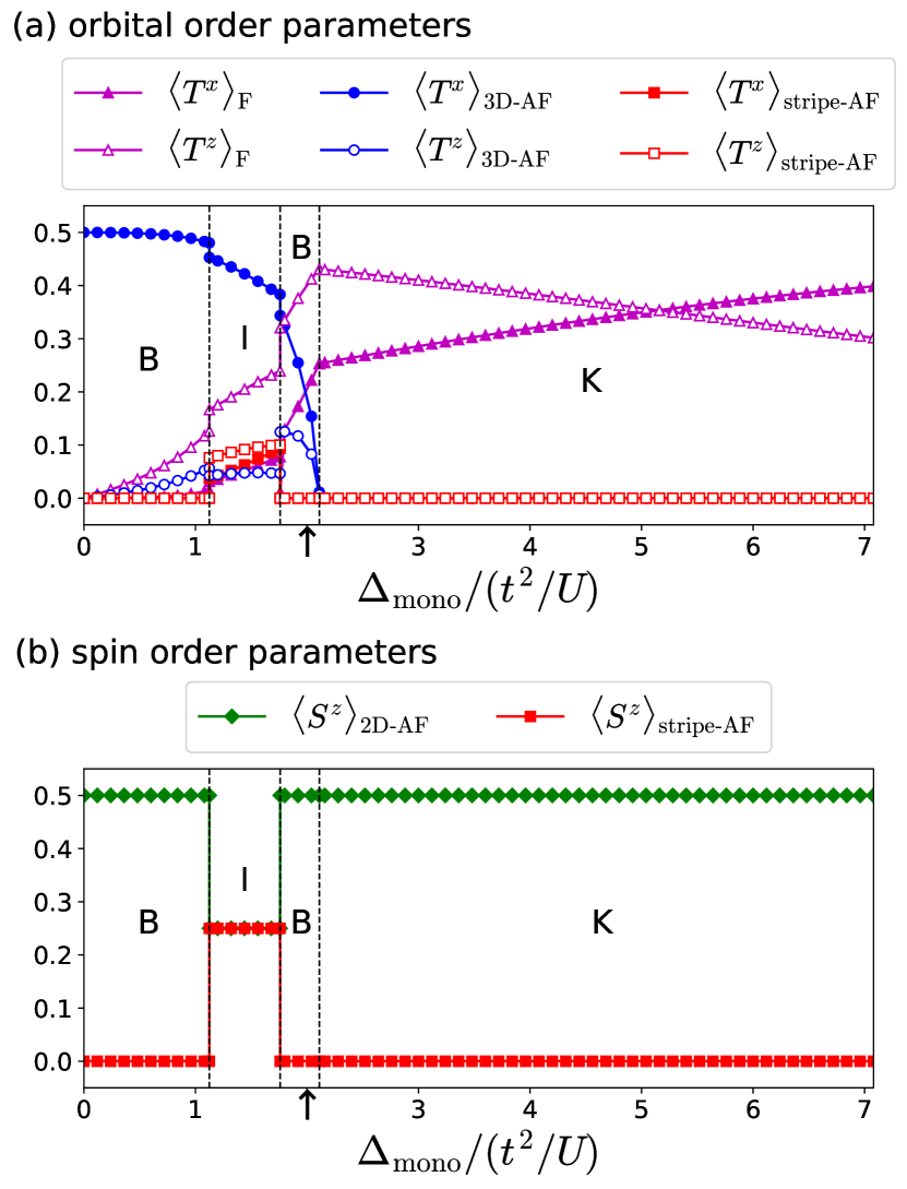
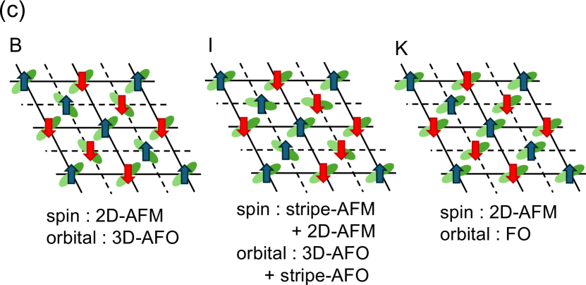
Figure 16: (a) The orbital and (b) spin order parameters in the monoclinic model as a function of $\Delta_{\mathrm{mono}}$ with fixed $\Delta_{\mathrm{ortho}}/\Delta_{\mathrm{mono}}=0.232$. The hopping parameter set (vi) in Table 2 was used. The arrow represents the DFT estimate for monoclinic RbO2, $\Delta_{\mathrm{mono}}/(t^{2}/U)=2.0$. (c) Schematic ordering patterns in the monoclinic model.

Figures 16 (a) and 16 (b) show the variations of the orbital and spin order parameters as a function of $\Delta_{\mathrm{mono}}$. The ordered states in the presence of monoclinic distortion are depicted in Fig. 16 (c). At $\Delta_{\mathrm{mono}}=0$, the ground state is phase B (3D-AFO + 2D-AFM order) in contrast to CsO2. In the middle region of $1.13\leq\Delta_{\mathrm{mono}}\leq 1.76$ in phase B, six orbital order parameters plotted in Fig. 16 (a) and two spin order parameters in Fig. 16 (b) appear as the first-order transition. This state corresponds to phase I, which appeared also in the case of the orthorhombic distortion. Further increasing $\Delta_{\mathrm{mono}}$, the forced FO ordered state with 2D-AFM order is stabilized (phase K). The difference from the orthorhombic case is that $\expectationvalue{T^{z}}_{\textrm{F}}$ begins to decrease in the large $\Delta_{\mathrm{mono}}$ region since the distortion is coupled with $\expectationvalue{T^{x}}_{\textrm{F}}$. Besides, under the monoclinic distortion, phase F^′ shown in Fig. 14 (c) does not appear. This is because $\expectationvalue{T^{z}}_{\textrm{F}}$ in the $z=1/2$ plane is unstable in the monoclinic CEF in Eq. (16).

The DFT estimate $\Delta_{\mathrm{mono}}=4.95$ meV is normalized to $\Delta_{\mathrm{mono}}/(t^{2}/U)=2.0$ using $t=95$ meV and $U=3.55$ eV [19]. This value is indicated by arrows in Figs. 16 (a) and 16 (b). We thus conclude that RbO2 is in phase B or phase K. In both cases, the spin structure is 2D-AFM, which is characterized by the translation vector $\bm{q}=(1/2,1/2,0)$.

IV.4 Finite temperature properties

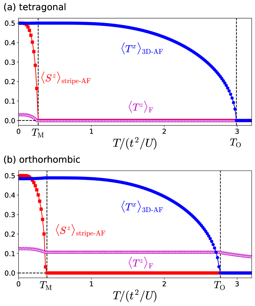
Figure 17: Temperature dependence of the order parameters in phase C. (a) The tetragonal parameter set (iv) in Table 2 and (b) the orthorhombic parameters (ii) with $\Delta_{\mathrm{ortho}}/(t^{2}/U)=0.60$ were used.

We conclude this section by presenting finite temperature properties. Figure 17 shows the temperature dependence of the order parameters in phase C. (a) is the result for the tetragonal model and (b) for the orthorhombic model with finite $\Delta_{\mathrm{ortho}}$. The order parameter for phase C is represented by $\expectationvalue{T^{x}}_{\textrm{3D-AF}}$ for the orbital part and $\expectationvalue{S^{z}}_{\textrm{stripe-AF}}$ for the spin part. We define the temperatures of the orbital and spin orders by $T_{\mathrm{O}}$ and $T_{\mathrm{M}}$, respectively. $T_{\mathrm{O}}$ is about six times higher than $T_{\mathrm{M}}$. This ratio depends on parameters such as $\theta$, $\phi$, and $J_{\mathrm{H}}/U$.

It is interesting that the canting of the orbital, represented by $\expectationvalue{T^{z}}_{\mathrm{F}}$, appears only below $T=T_{\mathrm{M}}$ in Fig. 17 (a). This means that the stripe-AFM order gives rise to the canting of the orbital. In fact, the direction of the stripe-AFM order and the canting of the orbital are correlated with each other. In the orthorhombic model in Fig. 17 (b), $\expectationvalue{T^{z}}_{\mathrm{F}}$ is finite in the whole temperature range because of the external orthorhombic distortion. $\expectationvalue{T^{z}}_{\mathrm{F}}$ exhibits a cusp at $T=T_{\mathrm{O}}$ and increases below $T=T_{\mathrm{M}}$, indicating that the stripe-AFM order enhances the orthorhombic distortion.

V Discussion

V.1 Role of the orbital degree of freedom

In this section, we first discuss the role of the orbital degree of freedom in our results. In particular, we focus on phase C (stripe-AFM + 3D-AFO order), which corresponds to the orthorhombic phase of CsO₂, and consider the origin of the phase transitions. The exchange interactions on all three kinds of bonds are relevant. The order of their strengths is $|J^{\mathrm{BC}}|>|J^{a}|\simeq|J^{a+b}|$ as shown in Fig. 6. The leading interaction $J^{\mathrm{BC}}$ leads to the 3D-AFO ordered state as demonstrated in the orbital-only model in Appendix B. The spin correlations are then considered on top of the 3D-AFO ordered state.

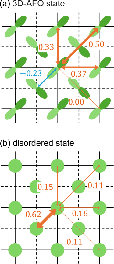
Figure 18: Values of the coupling constants, $J_{ij}$, in units of $t^{2}/U$ in the effective Heisenberg model in Eq. (17). The orange and blue indicate AFM and FM interactions, respectively. (a) 3D-AFO ordered state, (b) disordered state. The parameter set for the orthorhombic CsO2 in (ii) of Table 2 was used.

For this purpose, we derive the effective spin-spin interactions represented by the Heisenberg Hamiltonian

$$\mathcal{H}_{\mathrm{spin}}=\sum_{\langle ij\rangle}J_{ij}\bm{S}_{i}\cdot\bm{S}_{j},$$ (17)

by eliminating the orbital operators from $\mathcal{H}_{\mathrm{eff}}$ in Eq. (12). We estimate $J_{ij}$ by replacing the orbital operators $T_{i}^{z}$ and $T_{i}^{x}$ with their expectation values. In the 3D-AFO ordered state in phase C, for example, $T_{i}^{x}$ is replaced by $+1/2$ or $-1/2$ depending on the site and $T_{i}^{z}$ is replaced by 0 for all sites (the canting of the orbital is ignored). Figure 18 (a) shows the exchange interactions $J_{ij}$ obtained in the 3D-AFO ordered state. The leading interaction turns out to be the AFM interaction on the diagonal bond in the $a$-$b$ plane ($l=a+b$), which favors the stripe-AFM ordering [44, 45]. For comparison, we estimated $J_{ij}$ in the disordered state by replacing all orbital operators with zero in $\mathcal{H}_{\mathrm{eff}}$. The result is presented in Fig. 18 (b). The strengths of $J_{ij}$ in the disordered state are simply determined by the hopping amplitude. Therefore, $l=\textrm{BC}$ bond has the largest AFM interaction, which does not enhance the stripe-AFM order. The comparison between Figs. 18 (a) and (b) clearly demonstrates that the orbital order in the 3D-AFO ordered state is relevant for the emergence of the stripe-AFM state. Sensitivity of the magnetic order to the presence or absence of orbital order has been observed for RbO2 [20].

Finally, we consider the direction of the stripe-AFM state under the orthorhombic distortion. The external orthorhombic distortion with $a<b$ tilts the $\pi_{a+b}$ and $\pi_{a-b}$ orbitals to the $a$ axis (we again note that we are considering holes). Therefore, the interaction on the $a$ bond becomes predominant over the $b$ bond since the $a$ ($b$) bond is described more by $\pi$ ($\delta$) hopping under the distortion. The KK mechanism explains the AF spin configuration on the ferro-orbital configuration on the $a$ bond, which leads to the stripe-AFM order with the translation vector $\bm{q}=(1/2,0,0)$.

V.2 Implication for experiments

Recent neutron scattering experiments for CsO2 reported the stripe-AFM order with propagation vector $\bm{q}=(0,1/2,0)$ [14] or $\bm{q}=(1/2,0,0)$ [15] in the orthorhombic structure with $a<b$. Our results for phase C and other phases having the stripe-AFM ordered configuration exhibit $\bm{q}=(1/2,0,0)$ because the KK interaction on the $l=a$ bond favors $\bm{q}=(1/2,0,0)$ over $\bm{q}=(0,1/2,0)$ as discussed above.

The DFT estimate is located in phase C but close to phases A, B, I, and F^′ in the phase diagram in Fig. 15. Among those nearby phases, I and F^′ have the stripe-AFM configuration. However, it is not a pure stripe-AFM order but a stack of the stripe-AFM and the 2D-AFM orders. In these phases, neutron scattering experiments should observe not only $\bm{q}=(1/2,0,0)$ but also $\bm{q}=(1/2,1/2,0)$. Since the peak at $\bm{q}=(1/2,1/2,0)$ has not been observed, we exclude phases I and F^′ and propose only phase C as a candidate for CsO2.

Regarding RbO2, the spin structure has not been resolved experimentally (apart from a study of oxygen deficient RbO2 [46]). Our results in Fig. 16 predict phase B, namely, the 2D-AFM order with $\bm{q}=(1/2,1/2,0)$ on top of the 3D-AFO order, which is the same orbital order as in CsO2. In KO2, magnetic order occurs in the monoclinic phase which is beyond the scope of the present study. A previous theoretical study [18] discussed the 3D-AFO + 2D-AFM order (phase D in Fig. 10) for KO2 and RbO2. It is close to our DFT estimates, but in-plane hopping would need to be stronger for its realization.

We turn our attention to the finite-temperature properties in CsO2. Experimentally, there are three phase transitions, $T_{\mathrm{s1}}$, $T_{\mathrm{s2}}$, and $T_{\mathrm{N}}$, in phases II–III (Fig. 1). On the other hand, we obtained two phase transitions in phase C of our model: the stripe-AFM transition at $T_{\mathrm{M}}$ and the 3D-AFO order transition at $T_{\mathrm{O}}$ [Fig. 17 (a) for tetragonal structure and Fig. 17 (b) for orthorhombic structure]. The energy unit $J\equiv t^{2}/U$ is estimated to be $J\approx 21$ K using the DFT value $t=81$ meV for the orthorhombic CsO2 in (ii) of Table 2 and $U=3.55$ eV [19]. Hence, $T_{\mathrm{M}}$ and $T_{\mathrm{O}}$ in Fig. 17 (b) are converted to $T_{\mathrm{M}}\approx 8.4$ K and $T_{\mathrm{O}}\approx 59$ K. We identify $T_{\mathrm{M}}$ with $T_{\mathrm{N}}$ since the calculated magnetic structure and the transition temperature is consistent with the experiment. We further identify $T_{\mathrm{O}}$ with $T_{\mathrm{s2}}$ as presented in Fig. 19 since the AFO ordered state for $T_{\mathrm{M}}<T<T_{\mathrm{O}}$ does not give rise to a global lattice distortion as shown in Fig. 17 (a). The experimental structural phase transition from tetragonal to orthorhombic at $T=T_{\mathrm{s1}}$ is ascribed to an origin that is not considered in our effective model. Describing this transition would require a model that also includes lattice degrees of freedom.

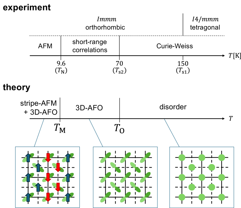
Figure 19: Comparison between the experimental and theoretical finite-$T$ phase diagrams.

In this scenario, the magnetic properties observed for $T_{\mathrm{N}}<T<T_{\mathrm{s2}}$ should be explained by the 3D-AFO ordered state. Experimentally, the temperature dependence of the susceptibility for $T_{\mathrm{N}}<T<T_{\mathrm{s2}}$ is well fitted by the Bonner-Fisher function [13, 11], which was developed to fit the one-dimensional Heisenberg model. In our model with O2–O2 hopping, none of the ordered states in Fig. 11 give a one-dimensional hopping path. We note that even the stripe-AFO ordered state proposed in Ref. [13] (e.g., $z=0$ plane in phase F) is not one-dimensional in the presence of the O2–O2 direct hopping. Considering the fact that the Bonner-Fisher curve of the susceptibility can be observed in a wide range of Heisenberg models [47], we expect that the susceptibility could be reproduced by the frustrated Heisenberg model on top of the 3D-AFO order as presented in Fig. 18 (a). For this, strong correlations and thermal fluctuations beyond the MF approximation need to be included which is beyond the scope of the present study.

The neutron diffraction experiment in Ref. [15] also suggests doubling of the unit cell along the $a$ axis for $T\leq T_{\rm s2}$, which is attributed to displacements of Cs and O₂ ions along the $b$ axis with the propagation vector $\bm{q}=(1/2,0,0)$. On the other hand, in the present calculation, the stripe-AFO order with $\bm{q}=(1/2,0,0)$ has not been obtained within the realistic parameter range. Therefore, this structural change is expected to originate from the instability of the background lattice system rather than the correlated $\pi$-electron system.

Finally, we refer to the experimental indication for the stripe-AFM + 3D-AFO ordered state of phase C in CsO₂. As shown in Fig. 17, the orbital order parameter $\expectationvalue{T^{z}}_{\mathrm{F}}$ corresponding to the orthorhombic distortion is enhanced below $T_{\rm M}$, accompanied by the development of the stripe-AFM order. This is because in phase C the orbital on each site tends to cant uniformly towards the $a$ axis to gain the AFM exchange interaction along the $a$ axis, parallel to the spin propagation vector. This canting of the orbital moment can be detected as the elongation and contraction of the $a$ and $b$ axes, respectively, as the temperature decreases through $T_{\rm N}$. This prediction provides a good validation of our scenario in experiments.

VI Summary

We investigated the spin-orbital order in $A$O2 ($A=\textrm{Cs}$, Rb, K) using a strong-coupling effective model derived based on first-principles calculations. Relevant interactions between the $\pi_{g}^{\ast}$ orbitals on the O2 molecule are up to third neighbor for tetragonal and up to fourth neighbor for orthorhombic structures. It is common to all $A$ atoms that the interaction between the corner and body-center sites ($l=\textrm{BC}$) is the largest. The difference in $A$ atoms can be seen in the $a$-$b$ plane. CsO2 has highly frustrated interactions between the $a$ ($b$) bond and the diagonal $a+b$ bond, while RbO2 and KO2 have weaker frustration. We conclude that a relevant microscopic control parameter that distinguishes the low-temperature properties in $A$O2 is the magnitude of the geometrical frustration in the $a$-$b$ plane ($\phi$ in our notation).

The MF calculations for the strong-coupling effective model reveal possible ground states in CsO2. Based on this, we propose a 3D-AFO order of $\pi_{a+b}$ and $\pi_{a-b}$ orbitals with the ordering vector $\bm{q}=(1,0,0)$. The orbital is canted towards the $a$ axis, which is consistent with the orthorhombic distortion. We predict that the canted orbital moment is enhanced, i.e., the lattice distortion increases, following the stripe-AFM transition to $\bm{q}=(1/2,0,0)$ order below $T_{\mathrm{N}}=9.6$ K.

The peculiar magnetic properties below $T=T_{\mathrm{s2}}$ in CsO2 remain unsolved in the present MF calculations. Our results suggest that the temperature dependence of the susceptibility fitted by the Bonner-Fisher curve should be explained by another mechanism such as geometrical frustration in systems with two or three dimensions. The fact that the observed magnetic moment is considerably reduced from $S=1/2$ indicates the importance of correlations in the magnetic properties, which is left for future work.

Appendix A Coupling constants

In this appendix, we compare the magnitude of the coupling constants defined in Eq. (13). The ratio between $J_{1}^{l}$, $J_{2}^{l}$, $J_{2}^{{}^{\prime}l}$, and $J_{3}^{l}$ is determined by the local interaction parameters. Figure 20 shows the ratios, $J_{2}^{l}/J_{1}^{l}$ and $J_{3}^{l}/J_{1}^{l}$ as a function of $J_{\mathrm{H}}/U$. Here, we use the relation $U^{\prime}=U-2J_{\mathrm{H}}$ and $J_{\mathrm{H}}^{\prime}=J_{\mathrm{H}}$ as in the main text. In this case, $J_{2}^{{}^{\prime}l}$ is identical to $J_{2}^{l}$, namely, $J_{2}^{{}^{\prime}l}=J_{2}^{l}$. Figure 20 demonstrates the inequality $J_{1}^{l}\geq J_{2}^{l}=J_{2}^{{}^{\prime}l}\geq J_{3}^{l}$. The equality holds when $J_{\mathrm{H}}/U=0$. For $J_{\mathrm{H}}/U=0.1$, for example, $J_{2}^{l}$ and $J_{3}^{l}$ are about 80% and 60% of $J_{1}^{l}$, respectively.

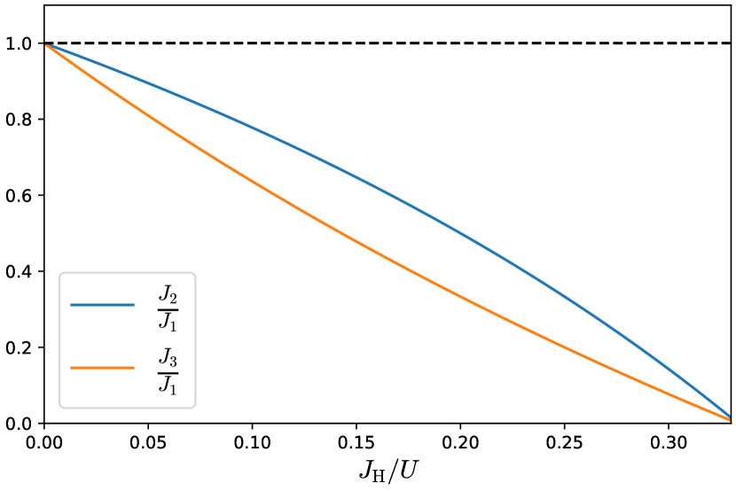
Figure 20: The ratios $J_{2}^{l}/J_{1}^{l}$ and $J_{3}^{l}/J_{1}^{l}$ as a function of $J_{\mathrm{H}}/U$.

Appendix B Orbital-only model

The effective Hamiltonian $\mathcal{H}_{\mathrm{eff}}$ in Eq. (12) consists of the spin and orbital operators. Here, we consider an orbital-only model by setting $\bm{S}_{i}=0$ in $\mathcal{H}_{\mathrm{eff}}$. Figure 21 shows the ground-state phase diagram of the orbital-only model in the $(\phi,\theta)$ plane. This figure explains the tendency of the orbital order in Fig. 10.

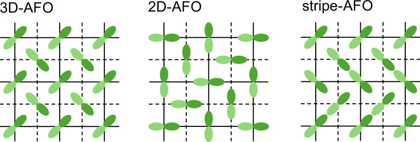
Figure 21: The ground-state phase diagram and orbital configuration in the orbital-only model. The parameters are the same as in Fig. 10.

There are three phases. The 3D-AFO state of the $(\pi_{a+b},\pi_{a-b})$ orbital is stabilized due to the interaction between the corner site and the body-center site, which is dominant near $\theta=0$. The region near $\theta=90^{\circ}$ is divided into two phases with a two-dimensional character. The 2D-AFO state of the $(\pi_{a},\pi_{b})$ orbital is stabilized below $\phi\simeq 53^{\circ}$ by the interaction along the $a$ axis and $b$ axis. The diagonal interaction in the $a$-$b$ plane, which is dominant near $\phi=90^{\circ}$, stabilizes the stripe-AFO order of the $(\pi_{a+b},\pi_{a-b})$ orbital.

Appendix C $J_{\mathrm{H}}/U$ dependence

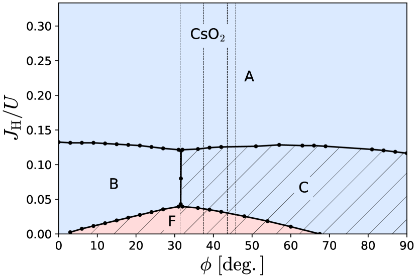
Figure 22: The ground-state phase diagram in $(\phi,J_{\mathrm{H}}/U)$ plane with $\theta=12.0^{\circ}$. The parameter set for the tetragonal CsO2 was used [(iv) in Table 2]. The vertical dashed lines indicate the DFT estimates of the $\phi$ value for CsO2 (see Table 2).

In the main text, $J_{\mathrm{H}}/U$ has been fixed at 0.1. In this appendix, we present how the phases change as $J_{\mathrm{H}}/U$ is varied. Figure 22 shows the phase diagram with $\phi$ and $J_{\mathrm{H}}/U$ on the axes. The value of $\theta$ is fixed at $\theta=12^{\circ}$ for the tetragonal CsO2. The cut of Fig. 22 at $J_{\mathrm{H}}/U=0.1$ corresponds to the horizontal cut of Fig. 10 at $\theta=12^{\circ}$. It turns out that $J_{\mathrm{H}}/U$ stabilizes phase A over phases B and C, whereas phase F appears when $J_{\mathrm{H}}/U$ is decreased. Comparison between Fig. 22 and Fig. 10 indicates that an increase of $J_{\mathrm{H}}/U$ corresponds to a decrease of $\theta$. This tendency can be understood as follows. As $J_{\mathrm{H}}/U$ increases, the $J_{1}^{l}$ term becomes dominant (Appendix A). Then, the simple KK-type ordered state is favored. In contrast, four interaction terms ($J_{1}^{l}$, $J_{2}^{l}$, $J_{2}^{{}^{\prime}l}$, and $J_{3}^{l}$) become relevant in the limit $J_{\mathrm{H}}/U\to 0$. Competition between different interaction terms favors rather complicated states such as phase F.

References

- Freiman and Jodl [2004] Y. Freiman and H. Jodl, Solid oxygen, Phys. Rep. 401, 1 (2004).
- Shimizu et al. [1998] K. Shimizu, K. Suhara, M. Ikumo, M. I. Eremets, and K. Amaya, Superconductivity in oxygen, Nature 393, 767 (1998).
- Hesse et al. [1989] W. Hesse, M. Jansen, and W. Schnick, Recent results in solid state chemistry of ionic ozonides, hyperoxides, and peroxides, Prog. Solid State Chem. 19, 47 (1989).
- Kováčik et al. [2012] R. Kováčik, P. Werner, K. Dymkowski, and C. Ederer, Rubidium superoxide: A -electron Mott insulator, Phys. Rev. B 86, 075130 (2012).
- Zumsteg et al. [1974] A. Zumsteg, M. Ziegler, W. Känzig, and M. Bösch, Magnetische und kalorische Eigenschaften von Alkali-Hyperoxid-Kristallen, Phys. Condens. Matter 17, 267 (1974).
- Bösch and Känzig [1975] M. Bösch and W. Känzig, Optische Eigenschaften und Elektronische Struktur von Alkali-Hyperoxid-Kristallen, Helv. Phys. Acta 48, 743 (1975).
- Ziegler et al. [1976] M. Ziegler, M. Rosenfelf, and W. Känzig, Strukturuntersuchungen an Alkalihyperoxiden, Helv. Phys. Acta. 49, 57 (1976).
- Labhart et al. [1979] M. Labhart, D. Raoux, W. Känzig, and M. A. Bösch, Magnetic order in -electron systems: Electron paramagnetic resonance and antiferromagnetic resonance in the alkali hyperoxides K, Rb, and Cs, Phys. Rev. B 20, 53 (1979).
- [9] M. Miyajima, Research on the correlation between electron magnetism and molecular arrangement/orbitral order of alkali superoxide \ceAO2, Ph.D. thesis, Okayama University (2021).
- Astuti et al. [2019] F. Astuti, M. Miyajima, T. Fukuda, M. Kodani, T. Nakano, T. Kambe, and I. Watanabe, Anionogenic magnetism combined with lattice symmetry in alkali-metal superoxide \ceRbO2, J. Phys. Soc. Jpn. 88, 043701 (2019).
- Miyajima et al. [2018] M. Miyajima, F. Astuti, T. Kakuto, A. Matsuo, D. P. Sari, R. Asih, K. Okunishi, T. Nakano, Y. Nozue, K. Kindo, I. Watanabe, and T. Kambe, Magnetism and high-magnetic field magnetization in alkali superoxide \ceCsO2, J. Phys. Soc. Jpn. 87, 063704 (2018).
- Smith et al. [1966] H. G. Smith, R. M. Nicklow, L. J. Raubenheimer, and M. K. Wilkinson, Antiferromagnetism in potassium superoxide \ceKO2, J. Appl. Phys. 37, 1047 (1966).
- Riyadi et al. [2012] S. Riyadi, B. Zhang, R. A. de Groot, A. Caretta, P. H. M. van Loosdrecht, T. T. M. Palstra, and G. R. Blake, Antiferromagnetic spin chain driven by -orbital ordering in , Phys. Rev. Lett. 108, 217206 (2012).
- Nakano et al. [2023] T. Nakano, S. Kontani, M. Hiraishi, K. Mita, M. Miyajima, and T. Kambe, Antiferromagnetic structure with strongly reduced ordered moment of p-electron in \ceCsO2, J. Phys.: Condens. Matter 35, 435801 (2023).
- Ewings et al. [2023] R. A. Ewings, M. Reehuis, F. Orlandi, P. Manuel, D. D. Khalyavin, A. S. Gibbs, A. D. Fortes, A. Hoser, A. J. Princep, and M. Jansen, Crystal and magnetic structure of cesium superoxide, Phys. Rev. B 108, 174412 (2023).
- Kováčik and Ederer [2009] R. Kováčik and C. Ederer, Correlation effects in -electron magnets: Electronic structure of \ceRbO2 from first principles, Phys. Rev. B 80, 140411(R) (2009).
- Ylvisaker et al. [2010] E. R. Ylvisaker, R. R. P. Singh, and W. E. Pickett, Orbital order, stacking defects, and spin fluctuations in the -electron molecular solid \ceRbO2, Phys. Rev. B 81, 180405(R) (2010).
- Wohlfeld et al. [2011] K. Wohlfeld, M. Daghofer, and A. M. Oleś, Spin-orbital physics for p orbitals in alkali ro2 hyperoxides—generalization of the goodenough-kanamori rules, Europhys. Lett. 96, 27001 (2011).
- Solovyev [2008] I. V. Solovyev, Spin–orbital superexchange physics emerging from interacting oxygen molecules in KO2, New J. Phys. 10, 013035 (2008).
- Nandy et al. [2010] A. K. Nandy, P. Mahadevan, P. Sen, and D. D. Sarma, : Realization of orbital ordering in a -orbital system, Phys. Rev. Lett. 105, 056403 (2010).
- Kim et al. [2010] M. Kim, B. H. Kim, H. C. Choi, and B. I. Min, Antiferromagnetic and structural transitions in the superoxide \ceKO2 from first principles: A -electron system with spin-orbital-lattice coupling, Phys. Rev. B 81, 100409(R) (2010).
- Kim and Min [2014] M. Kim and B. I. Min, Temperature-dependent orbital physics in a spin-orbital-lattice-coupled electron Mott system: The case of \ceKO2, Phys. Rev. B 89, 121106(R) (2014).
- Sikora et al. [2020] O. Sikora, D. Gotfryd, A. Ptok, M. Sternik, K. Wohlfeld, A. M. Oleś, and P. Piekarz, Origin of the monoclinic distortion and its impact on the electronic properties in \ceKO2, Phys. Rev. B 102, 085129 (2020).
- Klanjšek et al. [2015] M. Klanjšek, D. Arčon, A. Sans, P. Adler, M. Jansen, and C. Felser, Phonon-Modulated Magnetic Interactions and Spin Tomonaga-Luttinger Liquid in the -Orbital Antiferromagnet , Phys. Rev. Lett. 115, 057205 (2015).
- Knaflič et al. [2015] T. Knaflič, M. Klanjšek, A. Sans, P. Adler, M. Jansen, C. Felser, and D. Arčon, One-dimensional quantum antiferromagnetism in the -orbital \ceCsO2 compound revealed by electron paramagnetic resonance, Phys. Rev. B 91, 174419 (2015).
- Abrahams and Kalnajs [1955] S. C. Abrahams and J. Kalnajs, The crystal structure of -potassium superoxide, Acta Cryst. 8, 503 (1955).
- Koepernik and Eschrig [1999] K. Koepernik and H. Eschrig, Full-potential nonorthogonal local-orbital minimum-basis band-structure scheme, Phys. Rev. B 59, 1743 (1999).
- Perdew et al. [1996] J. P. Perdew, K. Burke, and M. Ernzerhof, Generalized gradient approximation made simple, Phys. Rev. Lett. 77, 3865 (1996).
- Koepernik et al. [2023] K. Koepernik, O. Janson, Y. Sun, and J. van den Brink, Symmetry-conserving maximally projected Wannier functions, Phys. Rev. B 107, 235135 (2023).
- Setyawan and Curtarolo [2010] W. Setyawan and S. Curtarolo, High-throughput electronic band structure calculations: Challenges and tools, Comput. Mater. Sci. 49, 299 (2010).
- [31] high symmetry points are , , , , , , , where and .
- [32] high symmetry points are , , , , , , , , where , , and .
- Slater and Koster [1954] J. C. Slater and G. F. Koster, Simplified LCAO method for the periodic potential problem, Phys. Rev. 94, 1498 (1954).
- Kugel’ and Khomskiĭ [1982] K. I. Kugel’ and D. I. Khomskiĭ, The Jahn-Teller effect and magnetism: transition metal compounds, Sov. Phys. Usp. 25, 231 (1982).
- Feiner et al. [1997] L. F. Feiner, A. M. Oleś, and J. Zaanen, Quantum melting of magnetic order due to orbital fluctuations, Phys. Rev. Lett. 78, 2799 (1997).
- Khaliullin and Oudovenko [1997] G. Khaliullin and V. Oudovenko, Spin and orbital excitation spectrum in the Kugel-Khomskii model, Phys. Rev. B 56, R14243 (1997).
- Okamoto et al. [2001] S. Okamoto, S. Ishihara, and S. Maekawa, Orbital structure and magnetic ordering in layered manganites: Universal correlation and its mechanism, Phys. Rev. B 63, 104401 (2001).
- Maekawa et al. [2004] S. Maekawa, T. Tohyama, S. E. Barnes, S. Ishihara, W. Koshibae, and G. Khaliullin, Physics of Transition Metal Oxides, Springer Series in Solid-State Sciences (Springer, 2004).
- Naka and Ishihara [2010] M. Naka and S. Ishihara, Electronic ferroelectricity in a dimer Mott insulator, J. Phys. Soc. Jpn. 79, 063707 (2010).
- Hotta [2010] C. Hotta, Quantum electric dipoles in spin-liquid dimer Mott insulator , Phys. Rev. B 82, 241104(R) (2010).
- Ghosh et al. [2019] P. Ghosh, T. Müller, F. P. Toldin, J. Richter, R. Narayanan, R. Thomale, J. Reuther, and Y. Iqbal, Quantum paramagnetism and helimagnetic orders in the Heisenberg model on the body centered cubic lattice, Phys. Rev. B 100, 014420 (2019).
- Kasamatsu et al. [2017] S. Kasamatsu, T. Kato, and O. Sugino, First-principles description of van der waals bonded spin-polarized systems using the vdW-DF+ method: Application to solid oxygen at low pressure, Phys. Rev. B 95, 235120 (2017).
- Landau et al. [1962] A. Landau, E. J. Allin, and H. Welsh, The absorption spectrum of solid oxygen in the wavelength region from 12,000 Å to 3300 Å, Spectrochimica Acta 18, 1 (1962).
- Jin et al. [2013] S. Jin, A. Sen, W. Guo, and A. W. Sandvik, Phase transitions in the frustrated Ising model on the square lattice, Phys. Rev. B 87, 144406 (2013).
- Glasbrenner et al. [2015] J. K. Glasbrenner, I. I. Mazin, H. O. Jeschke, P. J. Hirschfeld, R. M. Fernandes, and R. Valentí, Effect of magnetic frustration on nematicity and superconductivity in iron chalcogenides, Nat. Phys. 11, 953 (2015).
- Riyadi et al. [2011] S. Riyadi, S. Giriyapura, R. A. de Groot, A. Caretta, P. H. M. van Loosdrecht, T. T. M. Palstra, and G. R. Blake, Ferromagnetic order from p-electrons in rubidium oxide, Chem. Mater. 23, 1578 (2011).
- Zheng et al. [2005] W. Zheng, R. R. P. Singh, R. H. McKenzie, and R. Coldea, Temperature dependence of the magnetic susceptibility for triangular-lattice antiferromagnets with spatially anisotropic exchange constants, Phys. Rev. B 71, 134422 (2005).