Beamforming Design for Semantic-Bit Coexisting Communication System

Abstract

Semantic communication (SemCom) is emerging as a key technology for future sixth-generation (6G) systems. Unlike traditional bit-level communication (BitCom), SemCom directly optimizes performance at the semantic level, leading to superior communication efficiency. Nevertheless, the task-oriented nature of SemCom renders it challenging to completely replace BitCom. Consequently, it is desired to consider a semantic-bit coexisting communication system, where a base station (BS) serves SemCom users (sem-users) and BitCom users (bit-users) simultaneously. Such a system faces severe and heterogeneous inter-user interference. In this context, this paper provides a new semantic-bit coexisting communication framework and proposes a spatial beamforming scheme to accommodate both types of users. Specifically, we consider maximizing the semantic rate for semantic users while ensuring the quality-of-service (QoS) requirements for bit-users. Due to the intractability of obtaining the exact closed-form expression of the semantic rate, a data driven method is first applied to attain an approximated expression via data fitting. With the resulting complex transcendental function, majorization minimization (MM) is adopted to convert the original formulated problem into a multiple-ratio problem, which allows fractional programming (FP) to be used to further transform the problem into an inhomogeneous quadratically constrained quadratic programs (QCQP) problem. Solving the problem leads to a semi-closed form solution with undetermined Lagrangian factors that can be updated by a fixed point algorithm. Extensive simulation results demonstrate that the proposed beamforming scheme significantly outperforms conventional beamforming algorithms such as zero-forcing (ZF), maximum ratio transmission (MRT), and weighted minimum mean-square error (WMMSE).

I Introduction

According to Shannon and Weaver [1], communication could be classified into three levels, namely technical level concerning how accurately can the symbols of communication be transmitted, semantic level concerning how precisely do the transmitted symbols convey the desired meaning, and effectiveness level concerning how effectively does the received meaning affect conduct in the desired way. In the past forty years, researchers mainly focused on the first level design, driving the mobile communication system evolved from the first generation (1G) to the fifth generation (5G). The transmission rate has been significantly improved and the system capacity is gradually approaching the Shannon limit. However, the rapid growth of communication demand in modern society shows no signs of stopping. Specifically, the upcoming sixth generation (6G) is expected to achieve transmission rates that are ten times faster than those of 5G [2], which will enable the support of numerous new applications including virtual and augmented reality (VR/AR), smart factories, intelligent transportation systems, etc [3]. This thus prompts an active research area that rethinks the communication systems at the semantic even effectiveness level.

I-A Semantic Communication

To build communication systems at the semantic level, semantic communication (SemCom) that mines the semantic information from the source, is one of the most popular candidate technologies in 6G. Compared with the traditional bit-level digital communication (BitCom) framework that adopts separate source and channel coding (SSCC) for minimizing bit/symbol error rate, SemCom embraces joint source and channel coding (JSCC) through neural network, which enables the extraction of semantic information and demonstrates a better transmission efficiency compared with BitCom [4]. The authors in [5] proposed to use neural network to achieve JSCC for image recovery, and optimized the system performance through end-to-end learning under the criteria of mean square error (MSE). Then, the authors in [4] incorporated transformer and proposed DeepSC, which is shown to outperform BitCom, especially in the low signal-to-noise (SNR) regime. Based on these pioneering works [5, 4], SemCom has then been extensively studied under different data modalities, including image [6, 7], text [8], speech [9], video [10], and multimodal data [11]. Despite the potential performance gain of SemCom, critical concerns about its practical deployment remain. For example, most of the SemCom systems employ analog symbol transmission, while it has been verified that digital transmission is more reliable and secure, as well as cost-effective in hardware implementation. This prompts the development of digital SemCom by designing codebooks [12] and quantization methods [13, 14] for semantic information. Besides, the current SemCom heavily relies on neural networks, which are prone to overfitting the training data collected under certain limited scenarios and thus lack of generalization capability to deal with the challenges brought by the dynamic wireless environment. Prompted by this, authors in [15] proposed an attention-based JSCC scheme that uses channel-wise soft attention to scale features according to SNR conditions, which enables it applicable to scenarios with a broad range of SNRs through a single model. Then, given the multiple antenna cases, a channel-adaptive JSCC scheme that exploits the channel state information (CSI) and SNR through attention mechanism was further proposed in [16].

I-B Motivations

Although SemCom has shown great potential for 6G, there is a critical issue that requires further investigation: Can SemCom completely replace BitCom? We believe the answer is no. This is because the task-oriented nature of SemCom implies that it needs to be tailored for each specific task, which renders it not suitable for generic transmission tasks. As a result, we envision that future 6G network will see the co-existence of SemCom and BitCom, yielding the semantic-bit coexisting system that supports both SemCom users (sem-users) and BitCom users (bit-users). In the coexisting system, due to the diverse performance objectives, existing transmission schemes for BitCom can no longer provide satisfactory services for the sem-users, and thus need to be redesigned. In response to this, we investigate the beamforming design for the coexisting multi-user multiple-input single-output (MU-MISO) system, and try to shed lights on how to adapt the current transmission algorithms in BitCom to the coexisting system.

I-C Related works

The study of multiuser SemCom has received a lot of attention in recent years, which mainly lies in two directions: resource allocation and interference management. In terms of resource allocation, a semantic-aware channel assignment mechanism was proposed in [17], and an optimal semantic-oriented resource block allocation method was put forward in [18] subsequently. The main idea of these two works is adjusting communication resources for boosting the transmission of semantic information. On the other hand, multiuser usually accompanies with interference, which can cause semantic noise that significantly degrades the performance [19]. To mitigate the interference, several methods have been proposed. For instance, the authors in [20] proposed to jointly optimize the codebook and the decoder, as such the user interference could be minimized. The authors in [21] further proposed to dynamically fuse the semantic features to a joint latent representation and adjust the weights of different user semantic features to combat fading channels. In addition to the interference from other sem-users, the interference from bit-users needs to be appropriately mitigated as well. Given this, the coexistence of sem-users and bit-users was considered in the non-orthogonal multiple access (NOMA) system [22, 23], where bit-users and sem-users are viewed as primary users and secondary users, respectively. The interference issue was addressed through successive interference cancellation (SIC). However, in the case of MU-MISO that enables multi-users through spatial multiplexing, the coordination of the two types of users with diverse transmission objectives remains largely unexplored.

Beanforming is a key technique of MU-MISO systems and has been commonly-used for interference mitigation [24, 25, 26, 27, 28, 29, 30]. Several linear design methods have been proposed to tackle the beamforming problem in MU-MISO systems. Zero forcing (ZF) and maximum ratio transmission (MRT) algorithm are two simple but effective beamforming algorithms. The former minimizes the user interference, and the latter maximizes the signal gain at the destination user. Besides, a well-known iterative algorithm is the weighted minimum mean-square error (WMMSE) algorithm [24], which achieves high performance by first transforming the original problem into an MMSE problem and then updating the variables in an alternative manner. Given high complexity of the WMMSE algorithm and limited performance of the ZF and the MRT algorithm, researchers resort to deep learning for developing beamforming scheme with both low complexity and high performance. With the optimal solution structure revealed in [25], the data driven method that learns the undetermined parameters in the solution structure was proposed in [26], and further extended in [27]. Besides, the authors in [31] proposed to use deep unfolding of the WMMSE algorithm for MU-MISO downlink precoding, which constructs the iteration process in neural networks. Variants of the deep unfolding-based methods have been investigated in [28]. The aforementioned schemes aim to maximize the data rate for BitCom. However, recent research has revealed that the semantic rate in SemCom has a distinct mapping from SNR to performance [17, 22]. As a result, existing methods may not be suitable for the semantic-bit coexisting system, and a new beamforming scheme that takes into account the different transmission objectives is urgently needed.

I-D Contribution and Organization

In this paper, we investigate the transmission design for the semantic-bit coexisting paradigm in the multiple-antenna communication system. Specifically, we consider sem-users with the task of image transmission and propose an adaptive JSCC autoencoder for semantic information extraction and recovery. A data driven method is adopted to approximate the semantic rate of sem-users, based on which a beanforming problem that optimizes the performance of sem-users under the QoS constraints of bit-users is formulated and solved. The contributions of this paper are summarized as follows:

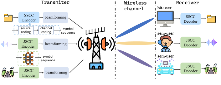
Figure 1: Semantic-bit coexisting communication system framework

• Targeting the task of image transmission, we propose an effective JSCC scheme that features a dynamic depth of downsampling, which is realized through the “early exit” mechanism [11] and the proposed module-by-module training scheme. On this basis, we further conduct semantic rate approximation on the ImageNet dataset and build the mapping from the depth of downsampling and SNR to semantic rate through data regression.

• We propose a beamforming design scheme for the semantic-bit coexisting system. Specifically, we tackle the primary challenge posed by the transcendental semantic rate function. By employing majorization-minimization (MM) and introducing a novel surrogate function, the original objective is transformed into a multiple-ratio form, which which is further converted to an inhomogeneous quadratically constrained quadratic programs (QCQP) problem by fractional programming. The semi-closed form solution for the resulting QCQP problem is derived, and the original problem is solved in an alternative manner. Additionally, the alternative algorithm has inspired a low-complexity beamforming method to address the complexity concern.

• Both theoretical analysis and numerical simulations are presented to validate the effectiveness of the proposed beamforming scheme in semantic-bit coexisting communication systems.

The rest of this paper is organized as follows. Section II introduces the semantic-bit coexisting system model. Section III presents the proposed JSCC design, the approximation of semantic rate, and the problem formulation. The optimization problem is solved in Section IV. Then, extensive simulation results are given in Section V, followed by the concluding remarks in Section VI.

II System Model

In this section, we first present the semantic-bit coexisting system and the transmission protocol, based on which the performance metrics of sem-users and bit-users are analyzed, respectively.

II-A Semantic-bit Coexisting Communication Framework

We consider a single-cell downlink multi-user multiple-input single-output (MU-MISO) system shown in Fig. 1. The base station (BS) is equipped with $N_{t}$ transmit antennas, while the users have a single antenna each. The users are divided into two groups, namely bit-users with BitCom and sem-users with SemCom. We denote the bit-users set as $\mathcal{B}=\{b_{1},b_{2},...,b_{B}\}$ and the sem-users set as $\mathcal{T}=\{t_{1},t_{2},...,t_{T}\}$, with $B$ and $T$ being the numbers of bit-users and sem-users, respectively. The transmit signal vector at the BS, denoted by $\mathbf{x}\in\mathbb{C}^{N_{t}\times 1}$, is given by

$$\mathbf{x}=\sum_{i=1}^{B}\mathbf{v}_{b_{i}}{s}_{b_{i}}+\sum_{j=1}^{T}\mathbf{v}_{t_{j}}s_{t_{j}},$$ (1)

where $\mathbf{v}_{b_{i}}\in\mathbb{C}^{N_{t}\times 1}$ and $\mathbf{v}_{t_{j}}\in\mathbb{C}^{N_{t}\times 1}$ denote the beamforming vector of the $i$-th bit-user and the $j$-th sem-user, respectively. Furthermore, we assume that $s_{b_{i}}$ and $s_{t_{j}}$ are zero mean and $\mathbb{E}[s_{b_{i}}s_{b_{i}}^{H}]=\mathbb{E}[s_{t_{j}}s_{t_{j}}^{H}]=1$, and the symbols desired for different users are independent from each other.

Then, the received signal $y_{b_{k}}\in\mathbb{C}$ at bit-user $b_{k}$ can be expressed as

$$y_{b_{k}}=\mathbf{h}_{b_{k}}^{H}\mathbf{v}_{b_{k}}s_{b_{k}}+\sum_{i=1,i\neq k}^{B}\mathbf{h}_{b_{k}}^{H}\mathbf{v}_{b_{i}}s_{b_{i}}\\ +\sum_{j=1}^{T}\mathbf{h}_{b_{k}}^{H}\mathbf{v}_{t_{j}}s_{t_{j}}+{n}_{b_{k}},\forall b_{k}\in\mathcal{B},$$ (2)

where $\mathbf{h}_{b_{k}}\in\mathbb{C}^{N_{t}\times 1}$ denotes the MISO channel from the BS to user $b_{k}$ and ${n}_{b_{k}}$ represents the additive noise which is modeled as a circularly symmetric complex Gaussian random variable following the distribution $\mathcal{CN}\big{(}\mathbf{0},\sigma_{b_{k}}^{2}\big{)}$, with $\sigma_{b_{k}}^{2}$ being the average noise power.

Similarly, let $\mathbf{h}_{t_{k}}\in\mathbb{C}^{N_{t}\times 1}$ denote the channel from the BS to the sem-user $t_{k}$, the received signal $y_{t_{k}}$ at sem-user $t_{k}$ is given by

$$y_{t_{k}}=\mathbf{h}_{t_{k}}^{H}\mathbf{v}_{t_{k}}s_{t_{k}}+\sum_{i=1}^{B}\mathbf{h}_{t_{k}}^{H}\mathbf{v}_{b_{i}}s_{b_{i}}\\ +\sum_{j=1,j\neq k}^{T}\mathbf{h}_{t_{k}}^{H}\mathbf{v}_{t_{j}}s_{t_{j}}+{n}_{t_{k}},\forall t_{k}\in\mathcal{T},$$ (3)

where ${n}_{t_{k}}$ is the additive white Gaussian noise with distribution $\mathcal{CN}(0,\sigma_{t_{k}}^{2})$. Notice that $s_{t_{j}}$ denotes the symbol stream that contains symbols in the latent representation, which is the output of the JSCC encoder. The symbols within the latent representation are transmitted sequentially.

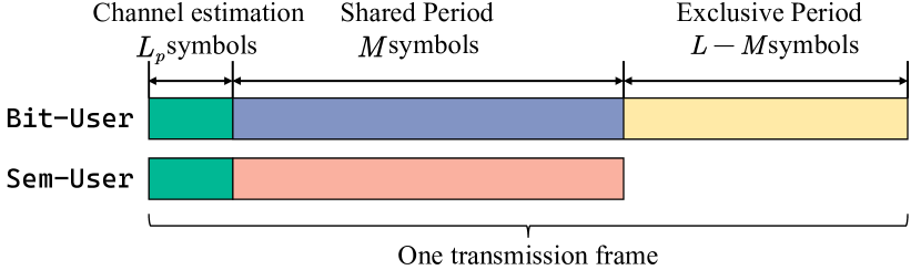
Figure 2: Transmission protocol for bit-users and sem-users

II-B Bit-level Communication

We adopt a transmission frame structure consisting of $L+L_{p}$ symbol intervals, as shown in Fig. 2. We assume slow fading channel, which means that the channel does not change within a frame and independently fades across different frames. In this vein, the first $L_{p}$ symbols are utilized for channel estimation and the remaining $L$ symbols for data transmission. With the estimated channel state information (CSI), the BS is able to conduct beamforming. It is worth noting that for sem-users, the target of transmission is to convey the latent representation from transmitter to receiver. Once this process completes, no further symbols are required. We assume sem-users should finish transmission of the latent representation in $M$ symbol intervals ($M<L$) and bit-users uses all $L$ symbol intervals for data transmission, which leads to the semi-non-orthogonal multiple access (semi-NOMA) [32]. In this context, the total data transmission component of length $L$ symbol intervals is further divided into two parts, as shown in Fig. 2. At the shared period of length $M$ symbol intervals, the BS simultaneously serves all users. Both bit-users and sem-users will be interfered by each other. The exclusive period of length $L-M$ symbol intervals is dedicated to data transmission for bit-users, i.e., $s_{t_{k}}=0,\forall t_{k}\in\mathcal{T}$. As digital transmission is employed at the bit-user, the achievable bit rate (bits/s/Hz) during the shared period is given by [1]

$$R_{{b_{i},1}}=\log_{2}\left(1+{\gamma}_{b_{i},1}\right),$$ (4)

where $\gamma_{b_{i},1}=\frac{|\mathbf{h}_{b_{i}}^{H}\mathbf{v}_{b_{i}}|^{2}}{\sum_{j\in\{\mathcal{B},\mathcal{T}\}/b_{i}}|\mathbf{h}_{b_{i}}^{H}\mathbf{v}_{j}|^{2}+\sigma_{b_{i}}^{2}}$ denotes the signal-to-interference-plus-noise ratio (SINR) of bit-user $b_{i}$ during the shared period.

Then, at the exclusive period, the BS only serves the bit-users, and the corresponding achievable bit rate is given by

$$R_{{b_{i},2}}=\log_{2}\left(1+{\gamma}_{b_{i},2}\right),$$ (5)

where $\gamma_{b_{i},2}=\frac{|\mathbf{h}_{b_{i}}^{H}\mathbf{v}_{b_{i}}|^{2}}{\sum_{j\in\{\mathcal{B}\}/b_{i}}|\mathbf{h}_{b_{i}}^{H}\mathbf{v}_{j}|^{2}+\sigma_{b_{i}}^{2}}$.

As a result, the overall normalized bit rate of the bit-user $b_{i}$ in a frame is defined as below.

$$R_{{b_{i}}}=\frac{M}{L}\log_{2}\left(1+{\gamma}_{b_{i},1}\right)+\frac{L-M}{L}\log_{2}\left(1+{\gamma}_{b_{i},2}\right).$$ (6)

II-C Semantic Communication

In semantic communication, the semantic rate no longer focuses on the symbol error rate, but on the quality of task completion. Fundamentally, the performance of semantic communication hinges on the effectiveness of the JSCC model and the wireless noise intensity. In this sense, the semantic rate can be generally expressed as

$$S_{t_{i}}=\epsilon(\boldsymbol{\Theta},\gamma_{t_{i}}),$$ (7)

where $\boldsymbol{\Theta}$ denotes the semantic model composed of deep neural networks (DNNs) that determines $M$ and the specific method for the extraction of semantic information, and $\gamma_{t_{i}}=\frac{|\mathbf{h}_{t_{i}}^{H}\mathbf{v}_{t_{i}}|^{2}}{\sum_{j\in\{\mathcal{B,T}\}/t_{i}}|\mathbf{h}_{t_{i}}^{H}\mathbf{v}_{j}|^{2}+\sigma_{t_{i}}^{2}}$ is the SINR of the sem-user $t_{i}$ at the shared period. In the context of image transmission scenario, $\epsilon(\boldsymbol{\Theta},\gamma_{t_{i}})$ is evaluated under the widely-adopted performance metric called structural similarity index measure (SSIM).

As mentioned, the overall semantic rate is determined by the adopted JSCC model and the transmission environment. The former represents the semantic compression and exploitation ability of the semantic communication, while the later determines the level of noise disturbation. However, semantic communication highly relies on neural networks for semantic extraction and recovery, the black-box nature of which hinders the theoretical analysis, making $\epsilon(\boldsymbol{\Theta},\gamma_{t_{i}})$ unable to be acquired precisely. A commonly adopted method for tackling this problem is data regression [22, 32, 17], which obtains the mapping from $\boldsymbol{\Theta}$ and $\gamma_{t_{i}}$ to $S_{t_{i}}$ through sufficient experimental instances and curve fitting, which will be further elaborated in the subsequent section.

III JSCC Design and Semantic Rate Approximation

In this section, we will elaborate on the design of semantic communication in detail. Considering the task of image transmission,we first present the proposed design of the JSCC model. Then, we conduct a series of experiments to evaluate the performance in different system settings. Building on this, we approximate the semantic rate with data regression. Finally, the problem that jointly optimizes the beamforming vectors and the downsampling depth is formulated.

III-A JSCC Network Characterization

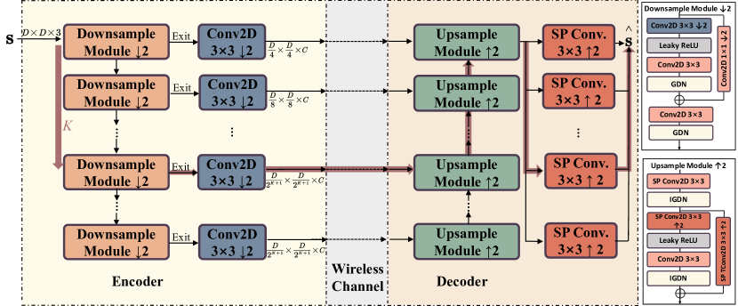
Figure 3: JSCC network for image transmission with multi exit mechanism

The proposed JSCC network for image transmission is shown in Fig. 3. At the encoder part, we consider compressing the original image $\mathbf{s}$ through multiple downsample modules $\mathcal{D}=\{\mathscr{D}_{n}\}_{n=1}^{N}$, each of which comprises a residual block [33], followed by a convolution layer. The number of filters in all the convolution layers is set to $C$. After each downsample module, the image size is reduced by half, and the number of channels is fixed to $C$. For the upsample module $\mathcal{U}=\{\mathscr{U}_{n}\}_{n=1}^{N}$ at the decoder part, the reverse process is conducted. Without loss of generality, we consider the image having a square size, that is, $\mathbf{s}\in\mathbb{R}^{D\times D\times 3}$, with $D$ being the image size, and “3” the number of channels, respectively.

Additionally, in typical 5G and beyond communication systems, due to the rapid growth in the number of users and data volumn, the BS needs to allocate communication resources to individual users. As a result, the available communication resources for users vary considerably in time and space, which poses new requirements for semantic communication. Specifically, the JSCC model should be able to dynamically adjust the number of the transmission symbols. To this end, we propose a multi-exit mechanism, as illustrated in Fig. 3. With this mechanism, the decoder can exit early rather than pass all the downsample modules. Consequently, the size of the latent representation can be adjusted by selecting the number of passed downsample module. Let $K$ be the number of passed downsample module, then the number of required transmission symbols $M_{K}$ is given by

$$M_{K}=C\big{(}\frac{D}{2^{K+1}}\big{)}^{2}=\frac{CD^{2}}{4^{K+1}}.$$ (8)

III-B Semantic Rate Approximation

Before deployment, training is required to obtain the JSCC neural network $\boldsymbol{\Theta}$. With the multi-exit mechanism, it is desired that the downsample and upsample modules in $\boldsymbol{\Theta}$ can work independently, and also be incorporated into deeper models (i.e., $\boldsymbol{\Theta}$ with a larger $K$). To this end, we propose a module-by-module training algorithm. As shown in Algorithm 1, the modules are trained sequentially, with only the weight parameters in the current layer modules being updated during the $K$-th round of training, while the upper layer modules (i.e., $\{\mathscr{D}_{n}\}_{n=1}^{K-1}$, $\{\mathscr{U}_{n}\}_{n=1}^{K-1}$) are frozen. Let $\boldsymbol{\Theta}_{K}$ be the JSCC model with a specific downsampling depth $K$. The semantic rate defined in (7) is given by $\epsilon(\boldsymbol{\Theta}_{K},\gamma)$, where $\gamma$ denotes the SNR. For simplicity, we use the notation $\epsilon(K,\gamma)$ for $\epsilon(\boldsymbol{\Theta}_{K},\gamma)$ in the rest of this paper, since $\boldsymbol{\Theta}_{K}$ is uniquely determined by $K$ when the downsampling and upsampling modules are specified.

Algorithm 1 Algorithm for Module-by-module Training

0:  all the modules including $\{\mathscr{D}_{M}\}_{M=1}^{N}$, $\{\mathscr{U}_{M}\}_{M=1}^{N}$.

1:  for $K=1,2,...,N$ do

2:     $\Theta=\{\{\mathscr{D}_{M}\}_{M=1}^{K},\{\mathscr{U}_{M}\}_{M=1}^{K}\}$.

3:     while $\Theta$ not converged do

4:        Sample a minibatch of data from training dataset

5:        Obtain the gradient $\nabla\mathscr{D}_{K}$ and $\nabla\mathscr{U}_{K}$ through loss calculation and backpropagation.

6:        Update $\mathscr{D}_{K}$ and $\mathscr{U}_{K}$ using $\mathscr{D}_{K}=\mathscr{D}_{K}-\eta\nabla\mathscr{D}_{K}$, $\mathscr{U}_{K}=\mathscr{U}_{K}-\eta\nabla\mathscr{U}_{K}$.

7:     end while

8:     Frozen $\mathscr{D}_{K}$ and $\mathscr{U}_{K}$.

9:  end for

We train $\boldsymbol{\Theta}$ on the ImageNet dataset [34], a large-scale image dataset containing over 14 million images, which serves as a standard benchmark for various computer vision tasks. For the channel setting, we consider the AWGN channel, where the SNR is fixed to 10 dB in the training process. Moreover, mean squared error (MSE) criteria is adopted as the loss function, and the Adam optimizer with the initiate learning rate of $10^{-4}$ is adopted. After sufficient training, we evaluate the performance $\epsilon(K,\gamma)$ on the validation dataset with different $K$ and SNR settings, under SSIM. The evaluation results are depicted in Fig. 4. It can be seen that with a increasing $K$, i.e., more stringent compression of the original image, the performance floor when ${\rm SNR}\rightarrow\infty$ decreases monotonically. Besides, for each $K$, $\epsilon(K,\gamma)$ follows an $S$ shape with respect to $\gamma$ in dB, which is also revealed in [22] under the text transmission task with the DeepSC model [4]. Therefore, similar to [22], the generalized logistic function could be utilized to well approximate $\epsilon(K,\gamma)$, as follows.

$$\epsilon(K,\gamma)\approx\tilde{\epsilon}(K,\gamma) =a_{K}+\frac{b_{K}}{c_{K}+{\rm exp}(-10d_{K}\log_{10}(\gamma))}$$

$$=a_{K}+\frac{b_{K}}{c_{K}+\gamma^{-\alpha_{K}}},$$ (9)

where $a_{K}$, $b_{K}$, $c_{K}$, $\alpha_{K}$ are parameters determined by $K$, and are obtained through curve fitting.

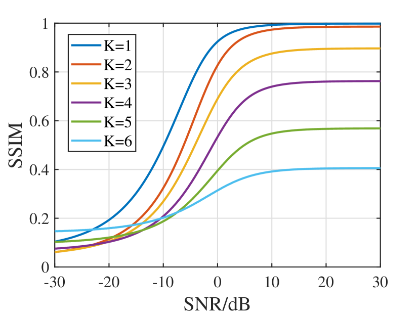
Figure 4: Performance evaluation under different $K$ and SNR settings

III-C Problem Formulation

As illustrated in Section II-A, there are two types of users with different performance metrics in the sematic-bit coexisting communication system. In this paper, we aim to maximize the semantic rate of sem-users while satisfying the QoS requirements of bit-users, by jointly optimizing the beamforming vectors and the downsampling depth. The considered optimization problem can be formulated as

$$\mathbf{P1}:\max_{\mathbf{V},K}\leavevmode\nobreak\ \leavevmode\nobreak\ \sum_{i=1}^{T}\tilde{\epsilon}\left(K,\gamma_{t_{i}}\right),$$ (10a)

$${\rm s.t.}\leavevmode\nobreak\ \leavevmode\nobreak\ \frac{M_{K}}{L}\log_{2}\left(1+\gamma_{b_{i},1}\right)+\frac{L-M_{K}}{L}$$

$$\qquad\leavevmode\nobreak\ \leavevmode\nobreak\ \leavevmode\nobreak\ \leavevmode\nobreak\ \cdot\log_{2}\left(1+\gamma_{b_{i},2}\right)\geq\beta_{b_{i}},\forall b_{i}\in\mathcal{B},$$ (10b)

$$\sum_{i=1}^{B}\left\|\mathbf{v}_{b_{i}}\right\|^{2}+\sum_{j=1}^{T}\left\|\mathbf{v}_{t_{j}}\right\|^{2}\leq P_{T},$$ (10c)

where $\gamma_{t_{i}}=\frac{|\mathbf{h}_{t_{i}}^{H}\mathbf{v}_{t_{i}}|^{2}}{\sum_{j\in\{\mathcal{B,T}\}/t_{i}}|\mathbf{h}_{t_{i}}^{H}\mathbf{v}_{j}|^{2}+\sigma_{t_{i}}^{2}}$, $\gamma_{b_{i},1}=\frac{|\mathbf{h}_{b_{i}}^{H}\mathbf{v}_{b_{i}}|^{2}}{\sum_{j\in\{\mathcal{B},\mathcal{T}\}/b_{i}}|\mathbf{h}_{b_{i}}^{H}\mathbf{v}_{j}|^{2}+\sigma_{b_{i}}^{2}}$, $\gamma_{b_{i},2}=\frac{|\mathbf{h}_{b_{i}}^{H}\mathbf{v}_{b_{i}}|^{2}}{\sum_{j\in\{\mathcal{B}\}/b_{i}}|\mathbf{h}_{b_{i}}^{H}\mathbf{v}_{j}|^{2}+\sigma_{b_{i}}^{2}}$, and $\mathbf{V}=[\mathbf{V}_{B},\mathbf{V}_{T}]\in\mathbb{C}^{N_{t}\times(B+T)}$, with $\mathbf{V}_{B}=[\mathbf{v}_{b_{1}},...,\mathbf{v}_{b_{B}}]\in\mathbb{C}^{N_{t}\times B}$ and $\mathbf{V}_{T}=[\mathbf{v}_{t_{1}},...,\mathbf{v}_{t_{T}}]\in\mathbb{C}^{N_{t}\times T}$. $\beta_{b_{i}}$ denotes the requirements of transmission rate in one frame from bit-user $b_{i}$. $P_{T}$ denotes the transmit power budget of the BS. $R_{b_{i},1}$ and $R_{b_{i},2}$ denote the transmission rate defined in (4) and (5), respectively. $\tilde{\epsilon}(K,\gamma_{t_{i}})$ is the approximated semantic rate given by (9).

Remark 1.

As shown in $\mathbf{P1}$, beamforming design for a semantic-bit coexisting system faces some new challenges compared to a BitCom system. Firstly, the semantic rate $\tilde{\epsilon}(K,\gamma_{t_{i}})$ admits a completely different form (which is neither convex nor concave) from channel capacity w.r.t. SINR, which renders the existing interference suppression algorithms ineffective. Additionally, the performance of sem-users also partially depends on the downsampling depth $K$ that requires careful design. Unfortunately, there exists a strong coupling between beamforming design and $K$, making the problem even more challenging to solve.

IV Joint Optimization of Beamforming and $K$-Configuring for Coexisting System

In this section, we solve the problem $\mathbf{P1}$ for beamforming design and configuring $K$ in semantic-bit coexisting MU-MISO systems. As discussed in Remark 1, it is hard to directly solve the joint optimization problem, and we thus consider solving $\mathbf{P1}$ by optimizing $\mathbf{V}$ and $K$ alternatively.

IV-A Beamforming Design

In this subsection, we optimize the beamforming matrix $\mathbf{V}$ in $\mathbf{P1}$ with a given $K$, and the subproblem is given below.

$$\mathbf{P2}:\max_{\mathbf{V}}\leavevmode\nobreak\ \leavevmode\nobreak\ \sum_{i=1}^{T}a_{K}+\frac{b_{K}}{c_{K}+(\gamma_{t_{i}})^{-\alpha_{K}}},$$ (11a)

$${\rm s.t.}\leavevmode\nobreak\ \leavevmode\nobreak\ (\ref{eq: qos constraints in p1}),(\ref{eq: power constraints in p1}).$$

As shown in $\mathbf{P2}$, the objective function (11a) is non-convex as (11a) is a transcendental function of $\mathbf{V}$. Moreover, the fractional expression exists in the QoS constraints. Therefore, $\mathbf{P2}$ is a NP-hard problem, indicating that the optimal solution is intractable. We thus resort to a suboptimal solution. To this end, the problem-solving process is mainly divided into four steps. Firstly, we relax the power constraint by regulating the noise intensity with ${{\rm Tr}(\mathbf{V}\mathbf{V}^{H})}/{P_{T}}$. Then, we propose a surrogate function for approximating the objective function. Next, the transforming method proposed in [36] is adopted to transform the multiple-ratio fractional programming (FP) problem into a QCQP problem. Finally, the resulting QCQP problem is solved in a low-complexity manner.

IV-A1 Problem Transformation

It can be observed that the beamforming vectors appear in $\mathbf{P}_{2}$ as the form of SINR in both the objective function (11a) and the QoS constraints (10b). Without loss of optimality, similar to [28, 37], the power constraint can be removed by integrating it to the SINR terms, as follows.

$$\mathbf{P3}:\max_{\mathbf{V}}\qquad \sum_{i=1}^{T}a_{K}+\frac{b_{K}}{c_{K}+(\Gamma_{t_{i}})^{-\alpha_{K}}},$$ (12a)

$${\rm s.t.}\qquad \frac{M_{K}}{L}\log_{2}\left(1+\Gamma_{b_{i},1}\right)+\frac{L-M_{K}}{L}$$

$$\qquad\cdot\log_{2}\left(1+\Gamma_{b_{i},2}\right)\geq\beta_{b_{i}},\forall b_{i}\in\mathcal{B}.$$ (12b)

where the equivalent SINR terms are given by

$$\Gamma_{t_{i}} =\frac{|\mathbf{h}_{t_{i}}^{H}\mathbf{v}_{t_{i}}|^{2}}{\sum_{j\in\{\mathcal{B,T}\}/t_{i}}|\mathbf{h}_{t_{i}}^{H}\mathbf{v}_{j}|^{2}+\frac{{\rm Tr}(\mathbf{V}\mathbf{V}^{H})}{P_{T}}\sigma_{t_{i}}^{2}},$$ (13)

$$\Gamma_{b_{i},1} =\frac{\left|\mathbf{h}_{b_{i}}^{H}\mathbf{v}_{b_{i}}\right|^{2}}{\sum_{j\in\left\{\mathcal{B},\mathcal{T}\right\}/b_{i}}\left|\mathbf{h}_{b_{i}}^{H}\mathbf{v}_{j}\right|^{2}+\frac{{\rm Tr}(\mathbf{V}\mathbf{V}^{H})}{P_{T}}\sigma_{b_{i}}^{2}},$$ (14)

$$\Gamma_{b_{i},2} =\frac{\left|\mathbf{h}_{b_{i}}^{H}\mathbf{v}_{b_{i}}\right|^{2}}{\sum_{j\in\left\{\mathcal{B}\right\}/b_{i}}\left|\mathbf{h}_{b_{i}}^{H}\mathbf{v}_{j}\right|^{2}+\frac{{\rm Tr}(\mathbf{V}\mathbf{V}^{H})}{P_{T}}\sigma_{b_{i}}^{2}}.$$ (15)

It can be found that the optimal solution $\mathbf{V}^{*}$ of the problem $\mathbf{P2}$ should satisfy the power constraint (10c) with equality. Then with the optimal solution $\mathbf{V}^{**}$ of the problem $\mathbf{P3}$, $\mathbf{V}^{*}$ can be obtained by $\sqrt{\frac{{P_{T}}}{{\rm Tr}(\mathbf{V}^{**}(\mathbf{V}^{**})^{H})}}\mathbf{V}^{**}$. Therefore, we can resort to solving $\mathbf{P3}$ for obtaining $\mathbf{V}^{*}$.

IV-A2 Objective Approximation

The goal is to transform the objective function (12a) such that the corresponding optimization problem can be appropriately solved. We adopt the idea of MM, that is, using a surrogate function to approximate the objective function (12a). Firstly, the semantic rate in $\mathbf{P3}$ is given by

$$\tilde{\epsilon}_{K}(\Gamma_{t_{i}})=a_{K}+\frac{b_{K}}{c_{K}+\Gamma_{t_{i}}^{-\alpha_{K}}}.$$ (16)

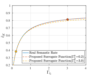
(a) $\alpha_{K}\leq 1$

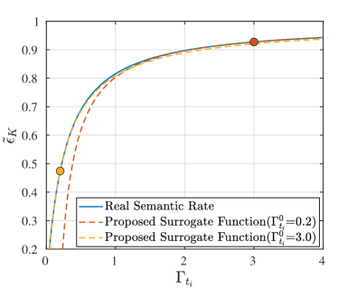
(b) $\alpha>1$

Figure 5: Objective Approximation with different surrogate functions

The exemplary functions with different $K$ settings are depicted in Fig. 5. Note that, our objective is to maximize the semantic rate w.r.t. the precoding matrix $\mathbf{V}$ rather than the SINR term $\{\Gamma_{t_{i}}\}$. Therefore, it is necessary to find an appropriate surrogate function that can accurately capture the shape of $\epsilon_{K}(\Gamma_{t_{i}})$ and also has a simple form for ease of handling during the optimization of $\mathbf{V}$. To this end, we propose to approximate $\tilde{\epsilon}_{K}(\cdot)$ with a surrogate function for the station point $\Gamma_{t_{i}}^{0}$ in each update round, as follows.

$$\zeta_{K}(\mathbf{V},\Gamma_{t_{i}}^{0})=D(K,\Gamma_{t_{i}}^{0})+E(K,\Gamma_{t_{i}}^{0})\frac{|\mathbf{h}_{t_{i}}^{H}\mathbf{v}_{t_{i}}|^{2}}{F(K,\Gamma_{t_{i}}^{0})|\mathbf{h}_{t_{i}}^{H}\mathbf{v}_{t_{i}}|^{2}+G(K,\Gamma_{t_{i}}^{0})(\sum_{j\in\{\mathcal{B,T}\}/t_{i}}|\mathbf{h}_{t_{i}}^{H}\mathbf{v}_{j}|^{2}+\frac{{\rm Tr}(\mathbf{V}\mathbf{V}^{H})}{P_{T}}\sigma_{t_{i}}^{2})},$$ (17)

 

$$\mathcal{J}(\Gamma_{t_{i}},{\Gamma_{t_{i}}^{0}},\alpha_{K})=\left\{\begin{aligned} \frac{1}{(\Gamma_{t_{i}}^{0})^{\alpha_{K}}}+\frac{\alpha_{K}}{(\Gamma_{t_{i}}^{0})^{\alpha_{K}-1}}(\frac{1}{\Gamma_{t_{i}}}-\frac{1}{\Gamma_{t_{i}}^{0}}),\alpha_{K}\leq 1\\ \frac{1}{\Gamma_{t_{i}}^{0}+\alpha_{K}(\Gamma_{t_{i}}^{0})^{\alpha-1}(\Gamma_{t_{i}}-\Gamma_{t_{i}}^{0}))},\alpha_{K}>1\end{aligned}\right.$$ (18)

Let $\zeta_{K}(\mathbf{V},\Gamma_{t_{i}}^{0})=a_{K}+\frac{b_{K}}{c_{K}+\mathcal{J}(\Gamma_{t_{i}},{\Gamma_{t_{i}}^{0}},\alpha_{K})}$, we have $\tilde{\epsilon}_{K}(\Gamma_{t_{i}})\geq\zeta_{K}(\mathbf{V},\Gamma_{t_{i}}^{0})$. Therefore we use $\zeta_{K}(\mathbf{V},\Gamma_{t_{i}}^{0})$ as the surrogate function for $\tilde{\epsilon}_{K}(\Gamma_{t_{i}})$. As shown in Fig. 5, the proposed surrogate function captured the original $\tilde{\epsilon}_{K}(\cdot)$ well, which leads to the following optimization problem:

$$\mathbf{P4}:\max_{\mathbf{V}} \sum_{i=1}^{T}\zeta_{K}(\mathbf{V},\Gamma_{t_{i}}^{0}),$$ (19a)

$${\rm s.t.}\qquad (\ref{eq: qos constraints in p3}).$$

It can be found that $\zeta_{K}(\cdot)$ exhibits a fractional form of $\Gamma_{t_{i}}$. Therefore, we resort $\zeta_{K}(\cdot)$ as a function of beamforming vectors, as shown in (17) on the top of this page, where $D(K,\Gamma_{t_{i}}^{0})=a_{K}$, $\qquad E(K,\Gamma_{t_{i}}^{0})=b_{K}$, $F(K,\Gamma_{t_{i}}^{0})=c_{K}+(1-\alpha_{K})(\Gamma_{t_{i}}^{0})^{-\alpha_{K}}$, and $G(K,\Gamma_{t_{i}}^{0})=\alpha_{K}(\Gamma_{t_{i}}^{0})^{1-\alpha_{K}}$ when $\alpha_{K}\leq 1$; $D(K,\Gamma_{t_{i}}^{0})=a_{K}+\frac{b_{K}(1-\alpha_{K})(\Gamma_{t_{i}}^{0})^{\alpha_{K}}}{c_{K}(1-\alpha_{K})(\Gamma_{t_{i}}^{0})^{\alpha_{K}}+1}$, $\qquad E(K,\Gamma_{t_{i}}^{0})=\frac{\alpha_{K}b_{K}(\Gamma_{t_{i}}^{0})^{\alpha_{K}-1}}{c_{K}(1-\alpha_{K})(\Gamma_{t_{i}}^{0})^{\alpha_{K}}+1}$, $F(K,\Gamma_{t_{i}}^{0})=\alpha_{K}c_{K}(\Gamma_{t_{i}}^{0})^{\alpha_{K}-1}$, and $G(K,\Gamma_{t_{i}}^{0})=c_{K}(1-\alpha_{K})(\Gamma_{t_{i}}^{0})^{\alpha_{K}}+1$ when $\alpha_{K}>1$.

Using the approximation method in each iteration, the problem is transformed into a multiple-ratio FP problem.

IV-A3 Fractional Programming

In this part, we solve the multiple-ratio FP problem $\mathbf{P4}$. Note that, $\mathbf{P4}$ still cannot be directly solved, because the QoS constraints are non-convex. Besides, in terms of the beamforming vector, both the objective and the constraints (12b) are in fractional form. To this end, the alternating optimization method is considered. We first apply the Lagrangian dual transformation proposed in [36] to (12b), and the problem can be equivalently written as

$$\mathbf{P5}:\max_{\mathbf{V},\mathbf{y},\mathbf{z}}\leavevmode\nobreak\ \leavevmode\nobreak\ \sum_{i=1}^{T}\zeta_{K}\big{(}\mathbf{V},\Gamma_{t_{i}}^{0}\big{)},$$ (20a)

$${\rm s.t.}\leavevmode\nobreak\ \leavevmode\nobreak\ \frac{M_{K}}{L}R_{b_{i},1}^{\prime}\big{(}y_{i},\mathbf{V}\big{)}$$

$$+\frac{L-M_{K}}{L}R_{b_{i},2}^{\prime}\big{(}z_{i},\mathbf{V}\big{)}\geq\beta_{b_{i}},\forall b_{i}\in\mathcal{B},$$ (20b)

where $\mathbf{y}=[y_{1},...,y_{B}]^{T}\in\mathbb{R}^{B}$, $\mathbf{z}=[z_{1},...,z_{B}]^{T}\in\mathbb{R}^{B}$ are auxiliary variables for the SINR terms,

$$R_{b_{i},1}^{\prime} =\log_{2}(1+y_{i})-y_{i}$$

$$\qquad\qquad+{\frac{(1+y_{i})|\mathbf{h}_{b_{i}}^{H}\mathbf{v}_{b_{i}}|^{2}}{\sum_{j\in\left\{\mathcal{B},\mathcal{T}\right\}}\left|\mathbf{h}_{b_{i}}^{H}\mathbf{v}_{j}\right|^{2}+\frac{{\rm Tr}(\mathbf{V}\mathbf{V}^{H})}{P_{T}}\sigma_{b_{i}}^{2}}},$$ (21)

$$R_{b_{i},2}^{\prime} =\log_{2}(1+z_{i})-z_{i}$$

$$\qquad\qquad+\frac{(1+z_{i})\left|\mathbf{h}_{b_{i}}^{H}\mathbf{v}_{b_{i}}\right|^{2}}{\sum_{j\in\left\{\mathcal{B}\right\}}\left|\mathbf{h}_{b_{i}}^{H}\mathbf{v}_{j}\right|^{2}+\frac{{\rm Tr}(\mathbf{V}\mathbf{V}^{H})}{P_{T}}\sigma_{b_{i}}^{2}}.$$ (22)

Note that, for maximizing $R_{b_{i},1}^{\prime}$ and $R_{b_{i},2}^{\prime}$ with a fixed $\mathbf{V}$, the optimal $\mathbf{y}$ and $\mathbf{z}$ equal to the corresponding SINR term of user $b_{i}$, as follows.

$$y_{i} =\frac{|\mathbf{h}_{b_{i}}^{H}\mathbf{v}_{b_{i}}|^{2}}{\sum_{j\in\{\mathcal{B,T}\}/b_{i}}|\mathbf{h}_{b_{i}}^{H}\mathbf{v}_{j}|^{2}+\frac{{\rm Tr}(\mathbf{V}\mathbf{V}^{H})}{P_{T}}\sigma_{b_{i}}^{2}},\leavevmode\nobreak\ i\in\{1,...,B\},$$ (23)

$$z_{i} =\frac{|\mathbf{h}_{b_{i}}^{H}\mathbf{v}_{b_{i}}|^{2}}{\sum_{j\in\{\mathcal{B}\}/b_{i}}|\mathbf{h}_{b_{i}}^{H}\mathbf{v}_{j}|^{2}+\frac{{\rm Tr}(\mathbf{V}\mathbf{V}^{H})}{P_{T}}\sigma_{b_{i}}^{2}},\leavevmode\nobreak\ \leavevmode\nobreak\ \leavevmode\nobreak\ \leavevmode\nobreak\ i\in\{1,...,B\}.$$ (24)

Moreover, $R^{\prime}_{b_{i},1}=R_{b_{i},1}$ and $R^{\prime}_{b_{i},2}=R_{b_{i},2}$ holds for optimal $\{y_{i}\}_{i=1}^{B}$ and $\{z_{i}\}_{i=1}^{B}$, respectively. The same properties holds for $R_{b_{i},2}^{{}^{\prime}}$ and $\mathbf{z}$ as well. Therefore, with the optimal $\mathbf{y}$ and $\mathbf{z}$, the problem $\mathbf{P5}$ can be reduced to

$$\mathbf{P6}:\max_{\mathbf{V}}\leavevmode\nobreak\ \leavevmode\nobreak\ \sum_{i=1}^{T}\zeta_{K}\big{(}\mathbf{V},\Gamma_{t_{i}}^{0}\big{)},$$ (25)

$${\rm s.t.}\leavevmode\nobreak\ \leavevmode\nobreak\ (\ref{eq: yz added QOS constraints}).$$

It can be found that in $\mathbf{P6}$, the sum-of-ratio form exists in both the objective and the QoS constraints. Therefore, we adopt the quadratic transformation proposed in [36], which yields the following optimization problem.

$$\mathbf{P7}:\max_{\mathbf{V},\mathbf{x},\mathbf{m},\mathbf{n}}\leavevmode\nobreak\ \leavevmode\nobreak\ \sum_{i=1}^{T}E(K,\gamma_{t_{i}}^{0})\bigg{[}2x_{i}{\rm Re}\{\mathbf{h}_{t_{i}}^{H}\mathbf{v}_{t_{i}}\}$$

$$-x_{i}^{2}\bigg{(}F(K,\gamma_{t_{i}}^{0})|\mathbf{h}_{t_{i}}^{H}\mathbf{v}_{t_{i}}|^{2}+G(K,\gamma_{t_{i}}^{0})$$

$$\cdot\big{(} \sum_{j\in\{\mathcal{B,T}\}/t_{i}}|\mathbf{h}_{t_{i}}^{H}\mathbf{v}_{j}|^{2}+\frac{{\rm Tr}(\mathbf{V}\mathbf{V}^{H})}{P_{T}}\sigma_{t_{i}}^{2}\big{)}\bigg{)}\bigg{]},$$ (26a)

$${\rm s.t.}\leavevmode\nobreak\ \leavevmode\nobreak\ \frac{M_{K}}{L}R_{b_{i},1}^{\prime\prime}(\mathbf{V},y_{i},m_{i})$$

$$+ \frac{L-M_{K}}{L}R_{b_{i},2}^{\prime\prime}(\mathbf{V},z_{i},n_{i})\geq\beta_{b_{i}},\forall b_{i}\in\mathcal{B},$$ (26b)

where $R_{b_{i},1}^{\prime\prime}(\mathbf{V},y_{i},m_{i})$ and $R_{b_{i},1}^{\prime\prime}(\mathbf{V},y_{i},m_{i})$ are given by

$$R_{b_{i},1}^{\prime\prime}(\mathbf{V},y_{i},m_{i}) =\log\left(1+y_{i}\right)-y_{i}+2m_{i}\sqrt{1+y_{i}}{\rm Re}\{\mathbf{h}_{b_{i}}^{H}\mathbf{v}_{b_{i}}\}$$

$$-m_{i}^{2}\big{(}\sum_{j\in\{\mathcal{B,T}\}}|\mathbf{h}_{b_{i}}^{H}\mathbf{v}_{j}|^{2}+\frac{{\rm Tr}(\mathbf{V}\mathbf{V}^{H})}{P_{T}}\sigma_{b_{i}}^{2}\big{)},$$ (27)

$$R_{b_{i},2}^{\prime\prime}(\mathbf{V},z_{i},n_{i}) =\log\left(1+z_{i}\right)-z_{i}+2n_{i}\sqrt{1+z_{i}}{\rm Re}\{\mathbf{h}_{b_{i}}^{H}\mathbf{v}_{b_{i}}\}$$

$$\leavevmode\nobreak\ \leavevmode\nobreak\ \leavevmode\nobreak\ -n_{i}^{2}\big{(}\sum_{j\in\{\mathcal{B}\}}|\mathbf{h}_{b_{i}}^{H}\mathbf{v}_{j}|^{2}+\frac{{\rm Tr}(\mathbf{V}\mathbf{V}^{H})}{P_{T}}\sigma_{b_{i}}^{2}\big{)}.$$ (28)

In $\mathbf{P7}$, three auxiliary vectors $\mathbf{x}=[x_{1},...,x_{T}]$, $\mathbf{m}=[m_{1},...,m_{B}]$, and $\mathbf{n}=[n_{1},...,n_{B}]$ are introduced to transform the original problem to a quadratic programming problem. More specifically, with a given $\mathbf{V}$, the optimal $\mathbf{x}$, $\mathbf{m}$, and $\mathbf{n}$ for $\mathbf{P7}$ are given as follows.

$$x_{i} ={\rm Re}\{\mathbf{h}_{t_{i}}^{H}\mathbf{v}_{t_{i}}\}\bigg{[}F(K,\Gamma_{t_{i}}^{0})|\mathbf{h}_{t_{i}}^{H}\mathbf{v}_{t_{i}}|^{2}+G(K,\Gamma_{t_{i}}^{0})$$

$$\cdot {\big{(}\sum_{j\in\{\mathcal{B,T}\}/t_{i}}|\mathbf{h}_{t_{i}}^{H}\mathbf{v}_{j}|^{2}+\frac{{\rm Tr}(\mathbf{V}\mathbf{V}^{H})}{P_{T}}\sigma_{t_{i}}^{2}\big{)}}\bigg{]}^{-1},\forall i=\{1,...,T\},$$ (29)

$$m_{i} =\frac{\sqrt{1+y_{i}}{\rm Re}\{\mathbf{h}_{b_{i}}^{H}\mathbf{v}_{b_{i}}\}}{\sum_{j\in\{\mathcal{B,T}\}}|\mathbf{h}_{b_{i}}^{H}\mathbf{v}_{j}|^{2}+\frac{{\rm Tr}(\mathbf{V}\mathbf{V}^{H})}{P_{T}}\sigma_{b_{i}}^{2}},\forall i=\{1,...,B\},$$ (30)

$$n_{i} =\frac{\sqrt{1+z_{i}}{\rm Re}\{\mathbf{h}_{b_{i}}^{H}\mathbf{v}_{b_{i}}\}}{\sum_{j\in\{\mathcal{B}\}}|\mathbf{h}_{b_{i}}^{H}\mathbf{v}_{j}|^{2}+\frac{{\rm Tr}(\mathbf{V}\mathbf{V}^{H})}{P_{T}}\sigma_{b_{i}}^{2}},\forall i=\{1,...,B\}.$$ (31)

Then, in terms of fixed $\mathbf{x}$, $\mathbf{m}$, and $\mathbf{n}$, the problem $\mathbf{P6}$ can be further reduced to

$$\mathbf{P8}:\max_{\mathbf{V}} \sum_{i=1}^{T}E(K,\gamma_{t_{i}}^{0})\bigg{[}2x_{t_{i}}{\rm Re}\{\mathbf{h}_{t_{i}}^{H}\mathbf{v}_{t_{i}}\}$$

$$-x_{t_{i}}^{2}\bigg{(}F(K,\Gamma_{t_{i}}^{0})|\mathbf{h}_{t_{i}}^{H}\mathbf{v}_{t_{i}}|^{2}+G(K,\Gamma_{t_{i}}^{0})$$

$$\big{(}\sum_{j\in\{\mathcal{B,T}\}/t_{i}}|\mathbf{h}_{t_{i}}^{H}\mathbf{v}_{j}|^{2}+\frac{{\rm Tr}(\mathbf{V}\mathbf{V}^{H})}{P_{T}}\sigma_{t_{i}}^{2}\big{)}\bigg{)}\bigg{]},$$ (32a)

$${\rm s.t.}\leavevmode\nobreak\ \leavevmode\nobreak\ (\ref{eq: qos constraints after fractional programming}).$$

It can be observed that $\mathbf{P8}$ is actually an inhomogeneous and separable QCQP problem, which can be solved by convex optimization toolboxes like CVX in MATLAB. However, the complexity of CVX is still unbearable since $\mathbf{P8}$ needs to be solved in each iteration. Therefore, we derive a semi-closed form solution for $\mathbf{P8}$ and propose a computationally efficient fixed point algorithm to search for the Lagrangian multipliers. Formally, the Lagrangian of $\mathbf{P8}$ is given by

$$\mathcal{L}(\mathbf{V},\boldsymbol{\lambda})= \sum_{i=1}^{T}E(K,\gamma_{t_{i}}^{0})\bigg{[}2x_{t_{i}}{\rm Re}\{\mathbf{h}_{t_{i}}^{H}\mathbf{v}_{t_{i}}\}$$

$$-x_{t_{i}}^{2}\bigg{(}F(K,\Gamma_{t_{i}}^{0})|\mathbf{h}_{t_{i}}^{H}\mathbf{v}_{t_{i}}|^{2}+G(K,\Gamma_{t_{i}}^{0})$$

$$\cdot\big{(}\sum_{j\in\{\mathcal{B,T}\}/t_{i}}|\mathbf{h}_{t_{i}}^{H}\mathbf{v}_{j}|^{2}+\frac{{\rm Tr}(\mathbf{V}\mathbf{V}^{H})}{P_{T}}\sigma_{t_{i}}^{2}\big{)}\bigg{)}\bigg{]}$$

$$+\sum_{i=1}^{B}\lambda_{i}\bigg{[}\frac{M_{K}}{L}R_{b_{i},1}^{\prime\prime}(\mathbf{V},y_{i},m_{i})$$

$$+\frac{L-M_{K}}{L}R_{b_{i},2}^{\prime\prime}(\mathbf{V},z_{i},n_{i})-\beta_{b_{i}}\bigg{]},$$ (33)

where $\boldsymbol{\lambda}=[\lambda_{1},...,\lambda_{B}]$ is the vector composed of multiple non-negative Lagrange multipliers.

By taking the first-order derivative of $\mathcal{L}$ over the precoding vectors (i.e., $\{\mathbf{v}_{t_{i}}\}_{i=1}^{T}$, $\{\mathbf{v}_{b_{i}}\}_{i=1}^{B}$) and setting it to zero, we have the following proposition.

Proposition 1.

For the MU-MISO system with channel $\{\{\mathbf{h}_{b_{i}}\}_{i=1}^{B},\{\mathbf{h}_{t_{i}}\}_{i=1}^{T}\}$, the optimal solution of the problem $\mathbf{P8}$ is given by

$$\mathbf{v}_{b_{i}} =\underbrace{\lambda_{i}\frac{M_{K}m_{i}\sqrt{1+y_{i}}+(L-M_{K})n_{i}\sqrt{1+z_{i}}}{L}}_{\rho_{b_{i}}}\mathbf{A}^{-1}\mathbf{h}_{b_{i}},$$ (34)

$${\rm where}\leavevmode\nobreak\ \mathbf{A}=\frac{\sum_{j=1}^{B}\mu_{j}\sigma_{b_{j}}^{2}+\sum_{j=1}^{T}\nu_{j}\sigma_{t_{j}}^{2}}{P_{T}}\mathbf{I}+\sum_{j=1}^{B}\mu_{j}\mathbf{h}_{b_{j}}\mathbf{h}_{b_{j}}^{H}$$

$$\qquad\qquad\qquad\qquad\qquad\qquad\qquad+\sum_{j=1}^{T}\nu_{j}\mathbf{h}_{t_{j}}\mathbf{h}_{t_{j}}^{H},$$ (35)

$$\mathbf{v}_{t_{i}} =\underbrace{x_{i}E(K,\Gamma_{t_{i}}^{0})}_{\varsigma_{t_{i}}}\mathbf{B}_{t_{i}}^{-1}\mathbf{h}_{t_{i}},\vspace{-10mm}$$ (36)

$${\rm where}\leavevmode\nobreak\ \mathbf{B}_{t_{i}}=\frac{\sum_{j=1}^{B}\mu_{j}\sigma_{b_{j}}^{2}+\sum_{j=1}^{T}\nu_{j}\sigma_{t_{j}}^{2}}{P_{T}}\mathbf{I}$$

$$+x_{i}^{2}E(K,\Gamma_{t_{i}}^{0})F(K,\Gamma_{t_{i}}^{0})\mathbf{h}_{t_{i}}\mathbf{h}_{t_{i}}^{H}+\sum_{j=1}^{B}\frac{\lambda_{j}M_{K}}{L}m_{j}^{2}\mathbf{h}_{b_{j}}\mathbf{h}_{b_{j}}^{H}$$

$$\qquad\qquad\qquad\qquad\qquad\qquad+\sum_{j=1,j\neq t_{i}}^{T}\nu_{j}\mathbf{h}_{t_{j}}\mathbf{h}_{t_{j}}^{H},$$ (37)

where $\mu_{j}=\frac{m_{j}^{2}\lambda_{j}M_{K}+n_{j}^{2}\lambda_{j}(L-M_{K})}{L}$, $\nu_{j}=x_{j}^{2}E(K,\Gamma_{t_{j}}^{0})G(K,\Gamma_{t_{j}}^{0})$.

Remark 2.

(Optimal Beamforming Structure) As shown in Proposition 1, it can be observed that the precoding vectors of both bit-users and sem-users are linear transformations of their corresponding channel vectors, where the weight coefficients is divided into linear power allocation coefficients (i.e., $\rho_{b_{i}}$ and $\varsigma_{t_{i}}$ in (34) and (36)) and priority coefficients for interference suppression (i.e., $\mu_{j}$, $\nu_{j}$, $\frac{\lambda_{j}M_{K}}{L}m_{j}^{2}$ in $\mathbf{A}$ and $\{\mathbf{B}_{t_{i}}\}_{i=1}^{T}$). Comparing (34) and (36), we can find that $\mathbf{v}_{t_{i}}$and $\mathbf{v}_{b_{i}}$ have different weight coefficients, indicating that sem-users have different resource allocation strategies compared to traditional digital communication due to their different objective functions. Furthermore, according to Proposition 1, the optimal precoding vector of $\mathbf{P8}$ is only determined by $\{\lambda_{i}\}_{i=1}^{B}$, so we can turn to find the optimal $\{\lambda_{i}\}_{i=1}^{B}$ for solving $\mathbf{P8}$, thereby reducing computational complexity.

Remark 3.

(Computation Complexity Analysis) For the calculation of $\{\mathbf{v}_{b_{i}}\}_{i=1}^{B}$, it can be observed that the inverse matrix is shared among bit-users, thus only needs to be calculated once. The complexity for calculating $\{\mathbf{v}_{b_{i}}\}_{i=1}^{B}$ is given by $\mathcal{O}(BN_{t}^{2}+TN_{t}^{2}+N_{t}^{3})$. For the calculation of $\{\mathbf{v}_{t_{i}}\}_{i=1}^{T}$, according to the Sherman–Morrison formula, we have $\mathbf{B}_{t_{i}}=(\mathbf{C}-\omega_{t_{i}}\mathbf{h_{t_{i}}\mathbf{h}_{t_{i}}^{H}})^{-1}=\mathbf{C}^{-1}+\omega_{t_{i}}\frac{\mathbf{C}^{-1}\mathbf{h}_{t_{i}}\mathbf{h}_{t_{i}}^{H}\mathbf{C}^{-1}}{1-\omega_{t_{i}}\mathbf{h}_{t_{i}}^{H}\mathbf{C}^{-1}\mathbf{h}_{t_{i}}}$, where $\mathbf{C}$ is defined in (38), and $\omega_{t_{i}}=\nu_{i}-x_{i}^{2}E(K,\Gamma_{t_{i}}^{0})F(K,\Gamma_{t_{i}}^{0})$. Therefore, the complexity for calculating $\{\mathbf{v}_{t_{i}}\}_{i=1}^{T}$ is given by $\mathcal{O}(BN_{t}^{2}+TN_{t}^{2}+N_{t}^{3})$. In a nutshell, the overall complexity for calculating the beamforming vectors by (34) and (36) is $\mathcal{O}(BN_{t}^{2}+TN_{t}^{2}+N_{t}^{3})$.

Algorithm 2 The proposed method for solving $\mathbf{P8}$

0:  $\boldsymbol{\lambda}=[\lambda_{1},...,\lambda_{B}]=0.01\times\mathbf{1},\boldsymbol{\lambda}^{\prime}=\mathbf{0}$.

1:  repeat

2:     Update $\boldsymbol{\lambda}^{\prime}$ by $\boldsymbol{\lambda}^{\prime}\leftarrow\boldsymbol{\lambda}$.

3:     Update precoding matrix $\mathbf{V}$ by (34), (36), and $\{\lambda_{i}\}_{i=1}^{B}$.

4:     Update $\{\lambda_{i}\}_{i=1}^{B}$ by (39).

5:  until $\sum_{i=1}^{B}|\lambda_{i}-\lambda_{i}^{\prime}|\leq\xi$

5:  the precoding matrix $\mathbf{V}$.

Algorithm 3 The proposed MM-FP algorithm for solving $\mathbf{P2}$

0:  the precoding matrix $\mathbf{V}$.

1:  repeat

2:     Update the SINR related terms, i.e., $\Gamma_{t_{i},0}\leftarrow\Gamma_{t_{i}}$, $\mathbf{y}$ with (23), $\mathbf{z}$ with (24).

3:     Update the ratio related terms, i.e., $\mathbf{x}$ with (29), $\mathbf{m}$ with (30), $\mathbf{n}$ with (31).

4:     Update the beamforming matrixes $\mathbf{V}$ by solving $\mathbf{P8}$ with Algorithm 2.

5:  until the objective value of $\mathbf{P2}$ converges or the iteration number reaches the maximum.

6:  Normalize the precoding matrix, i.e., $\mathbf{V}\leftarrow\sqrt{\frac{P_{T}}{{\rm Tr}(\mathbf{V}\mathbf{V}^{H})}}\mathbf{V}$.

$$\mathbf{C} =\frac{\sum_{j=1}^{B}\mu_{j}\sigma_{b_{j}}^{2}+\sum_{j=1}^{T}\nu_{j}\sigma_{t_{j}^{2}}}{P_{T}}\mathbf{I}+\sum_{j=1}^{B}\frac{\lambda_{j}M_{K}}{L}m_{j}^{2}\mathbf{h}_{b_{j}}\mathbf{h}_{b_{j}}^{H}+\sum_{j=1}^{T}\nu_{j}\mathbf{h}_{t_{j}}\mathbf{h}_{t_{j}}^{H},$$ (38)

$$\lambda_{i} =\frac{{\beta_{b_{i}}-\frac{M_{K}}{L}(\log(1+y_{i})-y_{i}-m_{i}^{2}\frac{{\rm Tr}(\mathbf{V}\mathbf{V}^{H})}{P_{T}}\sigma_{b_{i}}^{2})-\frac{L-M_{K}}{L}(\log(1+z_{i})-z_{i}-n_{i}^{2}\frac{{\rm Tr}(\mathbf{V}\mathbf{V}^{H})}{P_{T}}\sigma_{b_{i}}^{2})}}{{2(\frac{M_{K}}{L}m_{i}\sqrt{1+y_{i}}+\frac{L-M_{K}}{L}n_{i}\sqrt{1+z_{i}})^{2}}{\rm Re}\{\mathbf{h}_{b_{i}}^{H}\mathbf{A}^{-1}\mathbf{h}_{b_{i}}\}}$$

$$\qquad\qquad\qquad\qquad\qquad\qquad\qquad+\frac{\frac{M_{K}}{L}m_{i}^{2}\big{(}\sum_{j\in\{\mathcal{B,T}\}}|\mathbf{h}_{b_{i}}^{H}\mathbf{v}_{j}|^{2}\big{)}+\frac{L-M_{K}}{L}n_{i}^{2}\big{(}\sum_{j\in\{\mathcal{B}\}}|\mathbf{h}_{b_{i}}^{H}\mathbf{v}_{j}|^{2}\big{)}}{{2(\frac{M_{K}}{L}m_{i}\sqrt{1+y_{i}}+\frac{L-M_{K}}{L}n_{i}\sqrt{1+z_{i}})^{2}}{\rm Re}\{\mathbf{h}_{b_{i}}^{H}\mathbf{A}^{-1}\mathbf{h}_{b_{i}}\}}.$$ (39)

 

As discussed in Remark 2, to obtain the optimal solution of $\mathbf{P8}$, only the Lagrange multipliers $\{\lambda_{i}^{*}\}_{i=1}^{B}$ needs to be determined, where $\lambda_{i}^{*}$ denotes the optimal dual variable. In addition, it can be found that the optimal solution of $\mathbf{P8}$ should satisfy the QoS constraints with equality. As a result, we can obtain $\{\lambda_{i}^{*}\}_{i=1}^{B}$ by the fixed-point algorithm. The update rule is presented in (39). The solution process for $\mathbf{P8}$ is concluded in Algorithm 2.

So far, the problem $\mathbf{P2}$ has been solved in an alternating manner, which is summarized in Algorithm 3 and termed as majorization-minimization fractional programming (MM-FP). There are two groups of introduced variables, namely SINR related terms ($\{\gamma_{t_{i},0}\}_{i=1}^{T}$, $\mathbf{y}$, $\mathbf{z}$) and the fraction related terms ($\mathbf{x}$, $\mathbf{m}$, $\mathbf{n}$). As shown in (29)-(31), the two groups are updated in sequence, followed by the update of $\mathbf{V}$.

In addition, we propose a low-complexity beamforming method to address practicality concerns. Generally, beamforming involves determining the precoding direction and allocating power. As shown in (34) and (36), the precoding direction is determined by the channel vectors, $\{m_{i}\}_{I=1}^{B}$, $\{n_{i}\}_{I=1}^{B}$, $\{x_{i}\}_{I=1}^{B}$, and $\{\lambda_{i}\}_{I=1}^{B}$. Given this, we consider setting a uniform $\lambda_{i}$ for all bit-user $b_{i}$ for avoiding iteration, and approximating the value of $\{m_{i}\}_{I=1}^{B}$, $\{n_{i}\}_{I=1}^{B}$, $\{x_{i}\}_{I=1}^{B}$ by (29), (30), (31), where the precoding vectors are replaced by the corresponding channel vector. Consequently, the beamforming direction, denoted by $\{\widetilde{v}_{b_{i}}\}_{I=1}^{B},\{\widetilde{v}_{t_{i}}\}_{I=1}^{T}$, is established. Then we allocate the power by solving the following problem.

$$\mathbf{P9}:$$

$$\max_{\mathbf{p}_{T},\mathbf{p}_{B}}\sum_{i=1}^{T}a_{K}+\frac{b_{K}}{c_{K}+(\frac{p_{t_{i}}|\mathbf{h}_{t_{i}}^{H}\widetilde{\mathbf{v}}_{t_{i}}|^{2}}{(\sum_{j\in\{\mathcal{B,T}\}/t_{i}}p_{j}|\mathbf{h}_{t_{i}}^{H}\widetilde{\mathbf{v}}_{j}|^{2}+\sigma_{t_{i}}^{2})})^{-\alpha_{K}}},$$ (40a)

$${\rm s.t.}\frac{M_{K}}{L}\log_{2}\left(1+\frac{p_{b_{i}}\left|\mathbf{h}_{b_{i}}^{H}\widetilde{\mathbf{v}}_{b_{i}}\right|^{2}}{\sum_{j\in\left\{\mathcal{B},\mathcal{T}\right\}/b_{i}}p_{j}\left|\mathbf{h}_{b_{i}}^{H}\widetilde{\mathbf{v}}_{j}\right|^{2}+\sigma_{b_{i}}^{2}}\right)+\frac{L-M_{K}}{L}$$

$$\leavevmode\nobreak\ \leavevmode\nobreak\ \leavevmode\nobreak\ \cdot\log_{2}\left(1+\frac{p_{b_{i}}\left|\mathbf{h}_{b_{i}}^{H}\widetilde{\mathbf{v}}_{b_{i}}\right|^{2}}{\sum_{j\in\left\{\mathcal{B}\right\}/b_{i}}p_{j}\left|\mathbf{h}_{b_{i}}^{H}\widetilde{\mathbf{v}}_{j}\right|^{2}+\sigma_{b_{i}}^{2}}\right)\geq\beta_{b_{i}},\forall b_{i},$$ (40b)

$$\leavevmode\nobreak\ \leavevmode\nobreak\ \leavevmode\nobreak\ \leavevmode\nobreak\ \sum_{i=1}^{B}p_{b_{i}}+\sum_{j=1}^{T}p_{t_{j}}\leq P_{T}.$$ (40c)

where $\mathbf{p}_{T}=[p_{t_{1}},...,p_{t_{T}}]$ and $\mathbf{p}_{B}=[p_{b_{1}},...,p_{b_{B}}]$ denote the power allocation vectors of sem-users and bit-users, respectively.

The low-complexity majorization-minimization fractional programming (LP-MM-FP) algorithm is concluded in Algorithm 4.

Algorithm 4 The proposed LP-MM-FP algorithm for solving $\mathbf{P2}$

1:  $\lambda_{i}\leftarrow\lambda_{0}$, $i=1,...,B$.

2:  Calculate $\mathbf{m}$, $\mathbf{n}$, $\mathbf{x}$ ,$\{\Gamma_{t_{i}}\}_{i=1}^{T}$ by channel vectors and MRT precoding vectors (i.e., $\mathbf{v}_{t_{i}}=\frac{\mathbf{h}_{t_{i}}}{\|\mathbf{h}_{t_{i}}\|},\mathbf{v}_{b_{i}}=\frac{\mathbf{h}_{b_{i}}}{\|\mathbf{h}_{t_{i}}\|}$).

3:  Calculate the beamforming directions with $\{\lambda_{i}\}_{i=1}^{B}$ and $\{\Gamma_{t_{i}}\}_{i=1}^{T}$, i.e., $\widetilde{\mathbf{v}}_{t_{i}}=\frac{\mathbf{B}_{t_{i}}^{-1}\mathbf{h}_{t_{i}}}{\|\mathbf{B}_{t_{i}}^{-1}\mathbf{h}_{t_{i}}\|}$, $\widetilde{\mathbf{v}}_{t_{i}}=\frac{\mathbf{A}^{-1}\mathbf{b}_{t_{i}}}{\|\mathbf{A}^{-1}\mathbf{h}_{b_{i}}\|}$, where $\mathbf{A}$, $\mathbf{B}_{t_{i}}$ are given by (35) and (37), respectively.

4:  Calculate power allocation vectors $\mathbf{p}_{T}$ and $\mathbf{p}_{B}$ by solving problem $\mathbf{P9}$ with $\{\widetilde{\mathbf{v}}_{t_{i}}\}_{i=1}^{T}$ and $\{\widetilde{\mathbf{v}}_{b_{i}}\}_{i=1}^{B}$.

5:  Calculate the final precoding vectors by $\mathbf{v}_{t_{i}}=\sqrt{p_{t_{i}}}\widetilde{\mathbf{v}}_{t_{i}}$, $\mathbf{v}_{b_{i}}=\sqrt{p_{b_{i}}}\widetilde{\mathbf{v}}_{b_{i}}$.

Algorithm 5 The proposed beamforming algorithm for solving $\mathbf{P1}$

0:  The sample set $\mathcal{K}=\{K|K_{\rm min}\leq K\leq K_{\rm max},K\in\mathbb{Z}\}$

1:  for $K=K_{\min},...,K_{\rm max}$ in parallel do

2:     Obtain $\mathbf{V}_{K}$ through Algorihtm 3 with $K$.

3:     Calculate the objective value of problem denoted by $\mathbf{P1}$ $\tau(\mathbf{V}_{K},K)$ with $\mathbf{V}_{K}$ and $K$.

4:  end for

5:  $K_{\rm opt}=\arg\max_{K\in\mathcal{K}}{\tau(\mathbf{V}_{K},K)}$

5:  The beamforming matrix $\mathbf{V}_{K_{\rm opt}}$, $K_{\rm opt}$.

IV-B Overall Algorithm

In this subsection, we shall present the proposed method for solving the problem $\mathbf{P1}$. Firstly, the subproblem that optimizes the beamforming vector with a fixed $K$ has been tackled in a computation-efficient manner. Subsequently, recognising that the feasible set for $K$ (i.e., the downsampling depth) is typically constrained within a narrow integer range, we employ the exhaustive algorithm to identify the optimal $K$.

The overall algorithm is presented in Algorithm 5. It can be found that executing Algorithm 5 requires at most $K_{\rm max}-K_{\rm min}$ times the complexity of Algorithm 3, where $K_{\rm max}$ and $K_{\rm min}$ represent the maximum and minimum feasible values of $K$, respectively. For conducting Algorithm 3, it requires multiple iterations, each of which is divided into three steps. The first step includes the update of SINR related terms, with a complexity of $\mathcal{O}(BN_{t}+TN_{t})$; the second step includes the updates of the ratio related terms, with a complexity of $\mathcal{O}(BN_{t}+TN_{t})$; the third step includes the updates of precoding matrix, with a complexity of $\mathcal{O}(L_{2}(BN_{t}^{2}+TN_{t}^{2}+N_{t}^{3}))$, where $L_{2}$ denotes the the number of iteration rounds for the fixed point method. Therefore, the complexity for conducting Algorithm 3 is $\mathcal{O}(L_{1}L_{2}BN_{t}^{2}+L_{1}L_{2}TN_{t}^{2}+L_{1}N_{t}^{3})$, where $L_{1}$ denotes the iteration number of Algorithm 3. In conclusion, the complexity for conducting Algorithm 5 is given by $\mathcal{O}((K_{\rm max}-K_{\rm min})L_{1}L_{2}BN_{t}^{2}+(K_{\rm max}-K_{\rm min})L_{1}L_{2}TN_{t}^{2}+(K_{\rm max}-K_{\rm min})L_{1}N_{t}^{3})$.

V Numerical Results

V-A Simulation Setup

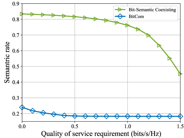
(a) Low SNR case (${\rm SNR}=0$ dB)

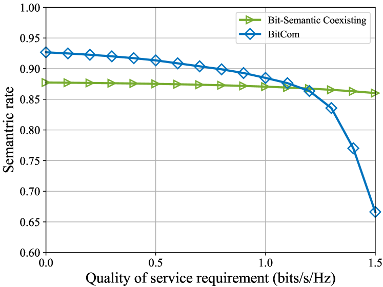
(b) High SNR case (${\rm SNR}=5$ dB)

Figure 6: Performance comparison of transmission systems

System setup. We consider the clustered Saleh-Valenzuela channel model [38], in which the channel from the BS to a specific user $i$ is given as follows.

$$\mathbf{h}_{i}=\frac{1}{\sqrt{L_{p}}}\sum_{l=1}^{L_{p}}\delta_{i,l}\mathbf{a}_{T}(\theta_{i,l}),$$ (41)

where $L_{p}$ is the number of paths and $\delta_{i,l}\sim\mathcal{CN}(0,1)$ is the channel attenuation of the $l$-th path. Without loss of generality, we set $L_{p}$ to $10$. $\theta_{i,l}$ denotes the azimuth angle of departure (AoD) at the transmitter, and we assume $\theta_{i,l}$ follows a uniform distribution from $0$ to $2\pi$. The response vector of Uniform Linear Array (ULA) at the BS side can be expressed as

$$\mathbf{a}_{T}(\theta_{i,l})=[1,e^{-j\pi\sin(\theta_{i,l})},...,e^{-j\pi(N_{t}-1)\sin(\theta_{i,l})}].$$ (42)

For the MISO system setting, unless specified, the following system parameters will be used as the default setting in the experiments: $N_{t}=16$, $B=5$, $T=3$, $K=3$, ${\rm SNR}=0$ dB, $\beta_{i}=1,\forall i$. Besides, as mentioned in Section III-B, the ImageNet dataset and SSIM are used as the training dataset and performance metric, respectively. The images are resized to $128\times 128$. The length of frame $L$ and the number of filters $C$ are set to $32,768$ and $128$, respectively. The downsampling depth $K\in\{K|2\leq K\leq 6,K\in\mathbb{Z}\}$. We also conduct performance evaluation on the Kodak image dataset, which comprises of 24 high-quality images.

Benchmark schemes. We compare the proposed beamforming algorithm, MM-FP and LP-MM-FP, with three commonly-adopted beamforming schemes, including the zero focing (ZF) algorithm, maximum ratio transmission (MRT) algorithm, and weighted minimum mean-square error (WMMSE) algorithm. Note that the aforementioned algorithms cannot be directly used for solving $\mathbf{P1}$, as the QoS constraints may not be satisfied. Given this, we first obtain the beamforming direction through these algorithms, i.e., $\widetilde{\mathbf{v}}_{i}={\mathbf{v}_{i}}/{\|\mathbf{v}_{i}\|_{2}},\forall i\in\mathcal{B}\cup\mathcal{T}$. Then we reallocate the power by solving the problem $\mathbf{P9}$, and the final beamforming vector is given by $\mathbf{v}_{i}=\sqrt{p_{i}}\widetilde{\mathbf{v}}_{i},\forall i\in\mathcal{B}\cup\mathcal{T}$. The resulting benchmark schemes are named ZF-PC, MRT-PC, and WMMSE-PC respectively.

V-B Evaluation of Coexisting System

In this subsection, we evaluate the effectiveness of the semantic-bit coexisting system. Firstly, we compare this system with the BitCom system. The semantic-bit coexisting system utilizes JSCC with neural network for image transmission, while the BitCom system enables image transmission through standard modular design, i.e., BPG for source coding, Turbo for channel coding, and 64QAM for modulation. The two different systems result in two sets of $\{a_{K},b_{K},c_{K},\alpha_{K}\}_{K=1}^{L}$, and we conduct Algorithm 3 for beamforming under the two parameter sets. The results are presented in Fig. 6, where Fig. 6(a) shows the performance in low SNR case (SNR = $0$dB), and Fig. 6(b) in high SNR case (SNR = $5$dB). In the low SNR case, the BitCom system fails to work under any of the examined QoS requirement. This is because BitCom is sensitive to noise. In the high SNR case, with a low QoS requirement, sem-users in the BitCom system enjoy low interference from bit-users, and thanks to the channel coding, the receiver is able to perfectly decode the BPG bit flow and attains good performance when $\beta_{i}\leq 0.5$. With the increase of QoS requirements, the strong interference causes the performance of BitCom to degrade quickly. In the meantime, the semantic-bit coexisting system only experiences a slight performance degradation as the QoS requirement increases from 0 to 1.5, thus demonstrating its effectiveness.

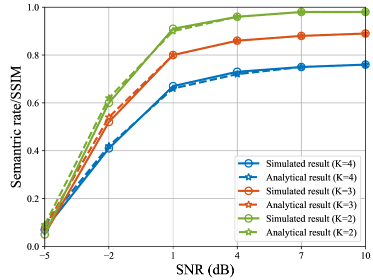
Figure 7: Validation of Semantic Rate Approximation

Since data driven method is used to approximate the semantic rate, it is important to compare the real semantic rate with the approximated one. We first implement the proposed beamforming scheme in Algorithm 3 and then compare the image recovery quality (i.e., SSIM) and the objective value in $\mathbf{P1}$. The performance comparison is presented in Fig. 7, where three different $K$ settings are considered. The final performance is averaged over $2,000$ test samples. As shown in Fig. 7, the approximation and simulation curves almost overlap, and the approximating-based method can well capture the performance growth trend as SNR increases. This validates the effectiveness of the data driven method in accurately approximating the semantic rate.

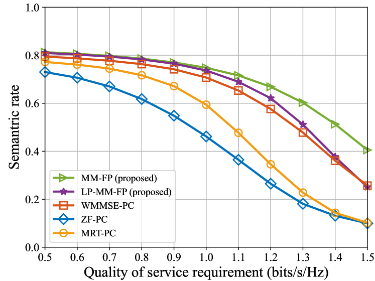
(a) ${\rm SNR=0}$ dB

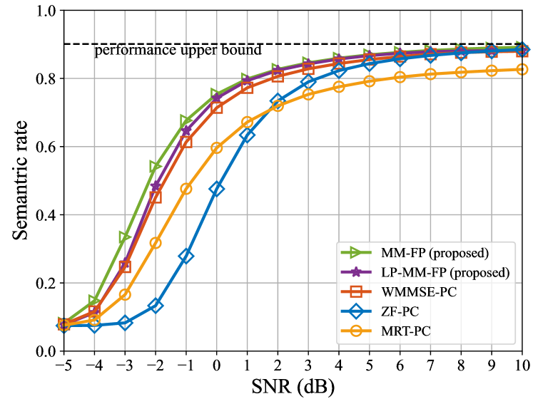
(b) $\beta_{i}=1,\forall i=1,...,B$

Figure 8: Performance comparison of different beamforming schemes

V-C Performance of Beamforming Design

In this subsection, we compare the performance of the proposed beamforming algorithm with three benchmark schemes. Fig. 8 depicts the semantic performance using different beamforming schemes in the coexisting system. We evaluate performance across different SNR and QoS settings. Under different QoS settings, Fig. 8(a) shows that heuristic beamforming schemes, such as ZF-PC and MRT-PC, perform poorly since they fail to coordinate beamforming direction and power for the problem $\mathbf{P2}$. The optimization-induced method WMMSE-PC achieves better performance than ZF-PC and MRT-PC. However, WMMSE-PC fails to consider the semantic objective in Fig. 4 and (9), which has a different mapping relationship between SNR and performance. As a result, the performance of WMMSE-PC degrades significantly when QoS requirements increase, which implies that tailored design of beamforming for coexisting systems is required. The proposed beamforming algorithm outperforms the three benchmark schemes in all QoS settings, achieving the best performance given all the examined QoS requirements. Moreover, the proposed LP-MM-FP algorithm achieves near performance with MM-FP algorithm especially in low QoS regime, while with much lower computational complexity. We also present some test examples in Fig. 10, where $\beta_{i}$ is set to 0.8. The recovered image from the system that adopts the ZF-PC or MRT-PC beamforming schemes has an obvious blur, which is also reflected in SSIM performance. The system with the WMMSE-PC algorithm has relatively more noise points in the first and third image. The system with the proposed beamforming scheme recovers the first and second image clearly, with some blurs in the third image, yet still outperforms the other three benchmark schemes in terms of SSIM.

Fig. 8(b) illustrates the performance comparison across different SNR settings. ZF-PC performs poorly in the low SNR regime, although it can approach the performance upper bound like WMMSE-PC and the proposed method when ${\rm SNR\geq 6}$ dB. MRT-PC performs relatively well in the low SNR regime, but the performance quickly degrades compared with other schemes as SNR increases since it does not consider user interference for beamforming design. Similarly, the proposed scheme outperforms these benchmark schemes in all the examined SNR settings, particularly in the low SNR regime, demonstrating its robustness. We present some test examples in Fig. 11, and the recovery performance is consistent with the analytical results in Fig. 8(b). The system that adopts the proposed beamforming scheme achieves the best SSIM performance in all three recovered images.

V-D Evaluation of $K$ Configuring Strategies

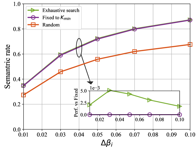
Figure 9: Performance comparison of different $K$-setting

This subsection evaluates the effectiveness of different methods for the configuration of $K$ in a typical loaded scenario, i.e., $N_{t}=16,\leavevmode\nobreak\ B=14,\leavevmode\nobreak\ T=1$. We compare the exhaustive search against two benchmark schemes: Random, which randomly selects a value of $K$ from $1$ to $L$; the best fixed $K$ setting, which we found to be the minimum value $K=2$ based on numerical experiments.We present the performance comparison in Fig. 9, where we use $\Delta\beta_{i}$ to denote the gap between the currently selected QoS value and the maximum achievable QoS, and a smaller $\Delta\beta_{i}$ indicates a more stringent QoS requirement. We observe that the performance of all schemes improves as $\Delta\beta_{i}$ increases, with the Random algorithm performing noticeably worse than the other three schemes. The fixed $K$ algorithm has already achives satisfactory performance in the transmission task considered in this paper, which can be adopted in the scenarios with limited computation capability. The considered method optimizes $K$ through the exhaustive method and can achieves the best performance.

Original	ZF-PC	MRT-PC	WMMSE-PC	MM-FP
SSIM	0.553	0.699	0.750	0.803
SSIM	0.717	0.642	0.766	0.851

Figure 10: Examples of reconstructed images under ${\rm SNR}=0$ dB, $\beta_{i}=0.8,\forall i=1,...,B$.

VI Conclusion

In this paper, we considered a semantic-user and bit-user coexisting system. A beamforming problem that maximizes the semantic rate under QoS constraints from bit-users and power constraint was formulated and solved in an low-complexity manner. Experiments show that the proposed method significantly improves the existing beamforming methods dedicated for BitCom. Addressing issues beyond beamforming in the coexisting system remains an interesting future direction.

Original	ZF-PC	MRT-PC	WMMSE-PC	MM-FP
SSIM	0.757	0.691	0.789	0.848
SSIM	0.781	0.475	0.827	0.844

Figure 11: Examples of reconstructed images under SNR=3dB, $\beta_{b_{i}}=1.0,\forall i=1,...,B$.

References

- [1] C. E. Shannon and W. Weaver, The mathematical theory of communication. University of illinois Press, 1949.
- [2] W. Jiang, B. Han, M. A. Habibi, and H. D. Schotten, “The road towards 6g: A comprehensive survey,” IEEE Open J. Commun. Soc., vol. 2, pp. 334–366, 2021.
- [3] W. Saad, M. Bennis, and M. Chen, “A vision of 6g wireless systems: Applications, trends, technologies, and open research problems,” IEEE Netw., vol. 34, no. 3, pp. 134–142, 2019.
- [4] H. Xie, Z. Qin, G. Y. Li, and B.-H. Juang, “Deep learning enabled semantic communication systems,” IEEE Trans. Singal Process., vol. 69, pp. 2663–2675, 2021.
- [5] E. Bourtsoulatze, D. B. Kurka, and D. Gündüz, “Deep joint source-channel coding for wireless image transmission,” IEEE Trans. Cogn. Commun. Netw., vol. 5, no. 3, pp. 567–579, 2019.
- [6] J. Dai, S. Wang, K. Tan, Z. Si, X. Qin, K. Niu, and P. Zhang, “Nonlinear transform source-channel coding for semantic communications,” IEEE J. Sel. Areas Commun., vol. 40, no. 8, pp. 2300–2316, 2022.
- [7] H. Gao, G. Yu, and Y. Cai, “Adaptive modulation and retransmission scheme for semantic communication systems,” IEEE Trans. Cogn. Commun. Netw., 2023.
- [8] P. Jiang, C.-K. Wen, S. Jin, and G. Y. Li, “Deep source-channel coding for sentence semantic transmission with HARQ,” IEEE transactions on communications, vol. 70, no. 8, pp. 5225–5240, 2022.
- [9] Z. Weng and Z. Qin, “Semantic communication systems for speech transmission,” IEEE J. Sel. Areas Commun., vol. 39, no. 8, pp. 2434–2444, 2021.
- [10] S. Wang, J. Dai, Z. Liang, K. Niu, Z. Si, C. Dong, X. Qin, and P. Zhang, “Wireless deep video semantic transmission,” IEEE J. Sel. Areas Commun., vol. 41, no. 1, pp. 214–229, 2022.
- [11] G. Zhang, Q. Hu, Z. Qin, Y. Cai, G. Yu, X. Tao, and G. Y. Li, “A unified multi-task semantic communication system for multimodal data,” [Online]. Available: https://arxiv.org/abs/2209.07689, 2022.
- [12] Q. Fu, H. Xie, Z. Qin, G. Slabaugh, and X. Tao, “Vector quantized semantic communication system,” IEEE Wireless Commun. Lett., 2023.
- [13] T.-Y. Tung, D. B. Kurka, M. Jankowski, and D. Gündüz, “Deepjscc-q: Constellation constrained deep joint source-channel coding,” IEEE J. Sel. Areas Inf. Theory, 2022.
- [14] Y. Bo, Y. Duan, S. Shao, and M. Tao, “Learning based joint coding-modulation for digital semantic communication systems,” [Online]. Available: https://arxiv.org/abs/2208.05704, 2022.
- [15] J. Xu, B. Ai, W. Chen, A. Yang, P. Sun, and M. Rodrigues, “Wireless image transmission using deep source channel coding with attention modules,” IEEE Trans. Circuits Syst. Video Technol., vol. 32, no. 4, pp. 2315–2328, 2021.
- [16] H. Wu, Y. Shao, K. Mikolajczyk, and D. Gündüz, “Channel-adaptive wireless image transmission with OFDM,” IEEE Wireless Commun. Lett., vol. 11, no. 11, pp. 2400–2404, 2022.
- [17] L. Yan, Z. Qin, R. Zhang, Y. Li, and G. Y. Li, “Resource allocation for text semantic communications,” IEEE Wireless Commun. Lett., vol. 11, no. 7, pp. 1394–1398, 2022.
- [18] C. Liu, C. Guo, Y. Yang, and N. Jiang, “Adaptable semantic compression and resource allocation for task-oriented communications,” [Online]. Available: https://arxiv.org/abs/2204.08910, 2022.
- [19] Q. Hu, G. Zhang, Z. Qin, Y. Cai, G. Yu, and G. Y. Li, “Robust semantic communications with masked VQ-VAE enabled codebook,” IEEE Trans. Wireless Commun., 2023.
- [20] M. Zhu, C. Feng, C. Guo, Z. Liu, N. Jiang, and O. Simeone, “Semantics-aware remote estimation via information bottleneck-inspired type based multiple access,” [Online]. Available: https://arxiv.org/abs/2212.09337, 2022.
- [21] T. Wu, Z. Chen, M. Tao, B. Xia, and W. Zhang, “Fusion-based multi-user semantic communications for wireless image transmission over degraded broadcast channels,” [Online]. Available: https://arxiv.org/abs/2305.09165, 2023.
- [22] X. Mu, Y. Liu, L. Guo, and N. Al-Dhahir, “Heterogeneous semantic and bit communications: A semi-NOMA scheme,” IEEE J. Sel. Areas Commun., vol. 41, no. 1, pp. 155–169, 2022.
- [23] W. Li, H. Liang, C. Dong, X. Xu, P. Zhang, and K. Liu, “Non-orthogonal multiple access enhanced multi-user semantic communication,” [Online]. Available: https://arxiv.org/abs/2303.06597, 2023.
- [24] Q. Shi, M. Razaviyayn, Z.-Q. Luo, and C. He, “An iteratively weighted MMSE approach to distributed sum-utility maximization for a MIMO interfering broadcast channel,” IEEE Trans. Singal Process., vol. 59, no. 9, pp. 4331–4340, 2011.
- [25] E. Björnson, M. Bengtsson, and B. Ottersten, “Optimal multiuser transmit beamforming: A difficult problem with a simple solution structure [lecture notes],” IEEE Signal Process. Mag., vol. 31, no. 4, pp. 142–148, 2014.
- [26] W. Xia, G. Zheng, Y. Zhu, J. Zhang, J. Wang, and A. P. Petropulu, “A deep learning framework for optimization of MISO downlink beamforming,” IEEE Trans. Commun., vol. 68, no. 3, pp. 1866–1880, 2019.
- [27] J. Kim, H. Lee, S.-E. Hong, and S.-H. Park, “Deep learning methods for universal MISO beamforming,” IEEE Wireless Commun. Lett., vol. 9, no. 11, pp. 1894–1898, 2020.
- [28] Q. Hu, Y. Cai, Q. Shi, K. Xu, G. Yu, and Z. Ding, “Iterative algorithm induced deep-unfolding neural networks: Precoding design for multiuser MIMO systems,” IEEE Trans. Wireless Commun., 2020.
- [29] L. Pellaco, M. Bengtsson, and J. Jaldén, “Matrix-inverse-free deep unfolding of the weighted MMSE beamforming algorithm,” IEEE Open J. Commun. Soc., vol. 3, pp. 65–81, 2021.
- [30] X. Hu, C. Liu, M. Peng, and C. Zhong, “Irs-based integrated location sensing and communication for mmwave simo systems,” IEEE Trans. Wireless Commun., 2022.
- [31] L. Pellaco, M. Bengtsson, and J. Jaldén, “Deep unfolding of the weighted MMSE beamforming algorithm,” [Online]. Available: https://arxiv.org/abs/2006.08448, 2020.
- [32] X. Mu and Y. Liu, “Exploiting semantic communication for non-orthogonal multiple access,” IEEE J. Sel. Areas Commun., 2023.
- [33] Z. Cheng, H. Sun, M. Takeuchi, and J. Katto, “Deep residual learning for image compression.,” in Proc. of the IEEE conference on computer vision and pattern recognition (CVPR), Long Beach, Canada, 2019.
- [34] J. Deng, W. Dong, R. Socher, L.-J. Li, K. Li, and L. Fei-Fei, “Imagenet: A large-scale hierarchical image database,” in Proc. IEEE Conference on Computer Vision and Pattern Recognition (CVPR), pp. 248–255, Miami, Florida, USA, 2009.
- [35] M. Zhang, Y. Li, Z. Zhang, G. Zhu, and C. Zhong, “Wireless image transmission with semantic and security awareness,” accepted to appear in IEEE Wireless Commun. Lett., 2023.
- [36] K. Shen and W. Yu, “Fractional programming for communication systems—Part I: Power control and beamforming,” IEEE Trans. Singal Process., vol. 66, no. 10, pp. 2616–2630, 2018.
- [37] X. Zhao, S. Lu, Q. Shi, and Z.-Q. Luo, “Rethinking WMMSE: Can its complexity scale linearly with the number of BS antennas?,” IEEE Trans. Singal Process., vol. 71, pp. 433–446, 2023.
- [38] J. Gao, C. Zhong, G. Y. Li, J. B. Soriaga, and A. Behboodi, “Deep learning-based channel estimation for wideband hybrid mmWave massive MIMO,” IEEE Trans. Commun., 2023.