Skyrmion on Magnetic Tunnel Junction: Interweaving Quantum Transport with Micro-magnetism

Abstract

Over the last two decades, non-trivial magnetic textures, especially the magnetic skyrmion family, have been extensively explored out of fundamental interest, and diverse possible applications. Given the possible technological and scientific ramifications of skyrmion-texture on magnetic tunnel junction (ST-MTJ), in this work, we present non-equilibrium Green’s function (NEGF) based description of ST-MTJs both for Néel and Bloch textures, to capture the spin/charge current across different voltages, temperatures, and sizes. We predict the emergence of a textured spin current from the uniform layer of the ST-MTJs, along with a radially varying, asymmetrical voltage dependence of spin torque. We delineate the voltage-induced rotation of the spin current texture, coupled with the appearance of helicity in spin current, particularly in the case of Néel skyrmions on MTJs. We describe the TMR roll-off in ST-MTJ with lower cross-sectional area and higher temperature based on transmission spectra analysis. We also introduce a computationally efficient coupled spatio-eigen framework of NEGF to address the 3D-NEGF requirement of the ST-MTJs. With analytical underpinning, we establish the generic nature of the spatio-eigen framework of NEGF, alleviating the sine-qua-non of the 3D-NEGF for systems that lack transnational invariance and simultaneous eigen-basis in the transverse directions.

I Introduction

The rise of topological magnetic textures such as merons, skyrmions, bimerons, antiskyrmions, skyrmioniums, hopfions, chiral bobbers to name a fewGobel et al. (2021), at the nano-scale has sparked a cascade of opportunities-from fundamental exploration to a myriad of practical applications. The magnetic skyrmionsMuhlbauer et al. (2009); Jonietz et al. (2010); Yu et al. (2010); Heinze et al. (2011); Hrabec et al. (2017), particularly notable for their stable vortex-like spin textures and nontrivial topology Nagaosa and Tokura (2013), have garnered significant attention for their technologically relevance. These micromagnetic structures manifest particle-like attributes attributed to their topological stability and nanometer-scale dimensions Wang et al. (2018). The combination of these characteristics, coupled with a low depinning current density, Romming et al. (2013) and the capability for electrical manipulation and detection Sampaio et al. (2013), positions magnetic skyrmions as highly auspicious candidates for the development of next-generation memory and processing devices. Consequently, many skyrmion based applications have been proposed such as nano-oscillators Garcia-Sanchez et al. (2016), racetrack memories Tomasello et al. (2014), logic gates Luo et al. (2018); Zhang et al. (2015a), neuromorphic computing Huang et al. (2017); Bhattacharya et al. (2019), and transistors Zhang et al. (2015b). Recent works Psaroudaki and Panagopoulos (2021); Psaroudaki et al. (2023) based on the quantization of the helicity have delineated the potential of skyrmions, merons Xia et al. (2022) and domain-wallsZou et al. (2023) for quantum computing. From a technological perspective, the electrical detection of skyrmions or magnetic textures via the tunnel magnetoresistance (TMR) in the magnetic tunnel junctions (MTJs) holds significant importance. The successful demonstration of nucleation and electrical detection of magnetic skyrmions in MTJs at room temperature Penthorn et al. (2019); He et al. (2023); Li et al. (2022); Kasai et al. (2019); Guang et al. (2023) marks a significant milestone in unlocking the potential of skyrmions. A uniform-textured (UT) MTJ comprises two ferromagnets (FMs) with uniform magnetization separated by an insulator (MgO) Butler et al. (2001), as depicted in Fig. 1(a). UT-MTJs have garnered significant attention primarily due to their notable TMR and spin transfer torque effect. Moreover, the early theoretical predictions unveiling the non-trivial voltage dependence of the spin current in UT-MTJs Slonczewski (1989); Theodonis et al. (2007) further elevated their importance. These revelations laid the groundwork for subsequent experimental validations Gosavi et al. (2017); Sun and Ralph (2008), sparking thorough investigations into device behavior. Moreover, these phenomena have not only inspired comprehensive studies but have also significantly influenced the design of various applications relying on UT-MTJsKim (2012); Sharma et al. (2017); Kultursay et al. (2013); van Dijken and Coey (2005); Sharma et al. (2016),. For the device like UT-MTJ, the Non-equilibrium Green’s Function (NEGF) based quantum transport Datta (1997), coupled with the Landau-Lifshitz-Gilbert (LLG) equation Slonczewski (1996), provides a robust framework for comprehending the dynamic interplay between charge/spin transport and magnetization dynamics of nano-magnet Salahuddin and Datta (2006); Sharma et al. (2017).

In the realm of magnetic textures, particularly concerning the dynamics of magnetic skyrmions, the micromagnetic framework based on the LLGS equation has been instrumental, leading to various innovative propositions for magnetic skyrmion devices. However, achieving a complete integrated understanding that merges micromagnetism and quantum transport on the same footing remains elusive, primarily due to unprecedented computational requirements.

Given the substantial technological implications associated with the skyrmion texture on the magnetic tunnel junctions (ST-MTJs), in this work, we present quantum transport interwoven with micromagnetic textures to capture the non-equilibrium dynamics of spin/charge current of ST-MTJs (Fig. 1(b)). Our work predicts the emergence of a textured spin current from the uniform top layer of ST-MTJs, accompanied by an asymmetrical voltage dependence. Additionally, we demonstrate a voltage-induced rotation of the spin current texture, coupled with the emergence of helicity, particularly observed in the case of Néel skyrmions.

To address the formidable task of solving the 3D-NEGF for the ST-MTJ, we introduce ‘spatio-eigen’ approach of the NEGF. The necessity for solving the 3D NEGF for the ST-MTJ arises due to the absence of translations symmetry and the lack of a simultaneous eigen basis of the contacts and channel along the transverse direction to the transport (refer to the methodology section). The computationally efficient spatio-eigen approach of NEGF is not limited to MTJ-like devices with skyrmions but is generic in nature, alleviating the need for 3D NEGF. This approach remains agnostic about the transnational symmetry and commutativity of the device Hamiltonian along the transverse direction.

Furthermore, we analytically demonstrate that the spatio-eigen approach of NEGF provides the same description of current flow while significantly reducing the size of matrices and the computational requirements, without compromising the physics. Utilizing the spatio-eigen approach of NEGF, we present an non-equilibrium description of the ST-MTJ, analyzing its spin and current profiles, as well as TMR, across varying voltages, temperatures and sizes.

II Methodology

In this section, we detail the non-equilibrium Green’s function (NEGF) based quantum transport coupled to micro-magnetism. We present two devices: the uniform magnetic textured magnetic tunnel junction (UT-MTJ) device, consisting of an insulating channel (MgO) sandwiched between two ferromagnetic (FM) layers with spatially uniform magnetization texture, and the magnetic skyrmion textured magnetic tunnel junction (ST-MTJ), in which one FM layer exhibits uniform magnetization, and the other layer features a magnetic Skyrmion, as depicted in Fig. 1. The current-voltage and spin current profile of these devices in principle can be obtained by the 3D-NEGF method. However this method requires a considerable amount of computing resources, making it practically unfeasible. The translation symmetry in the UT-MTJ along the orthogonal direction to the transport (i.e., $\hat{x}$ & $\hat{y}$ directions, see Fig. 1) allows for reduction of the complexity of quantum transport calculation by using Bloch expansion along the orthogonal direction Papior et al. (2017). But the absence of translation symmetry in ST-MTJ along the orthogonal direction breaks the notion of crystal momentum being a good quantum number, hence limiting the scope of Bloch expansion Ashcroft and Mermin (1976). Therefore, we introduce the spatio-eigen approach for NEGF-based quantum transport, which provides computational advantages over the full 3D-NEGF method. The spatio-eigen approach for NEGF can be applied in both cases, regardless of whether the system exhibits orthogonal translation symmetry along the direction perpendicular to the transport. In this approach of the NEGF decomposes, the Hamiltonian of the device is described in spatial basis (e.g., tight-binding or LCAO Papior et al. (2017)) along the transport direction and in the eigen basis along the orthogonal direction to the transport. We delineate both the decoupled and coupled spatio-eigen approaches of NEGF. Additionally, we provide analytical groundwork to illustrate that these approaches yield identical physics to that of the more computationally intensive full 3D-NEGF method

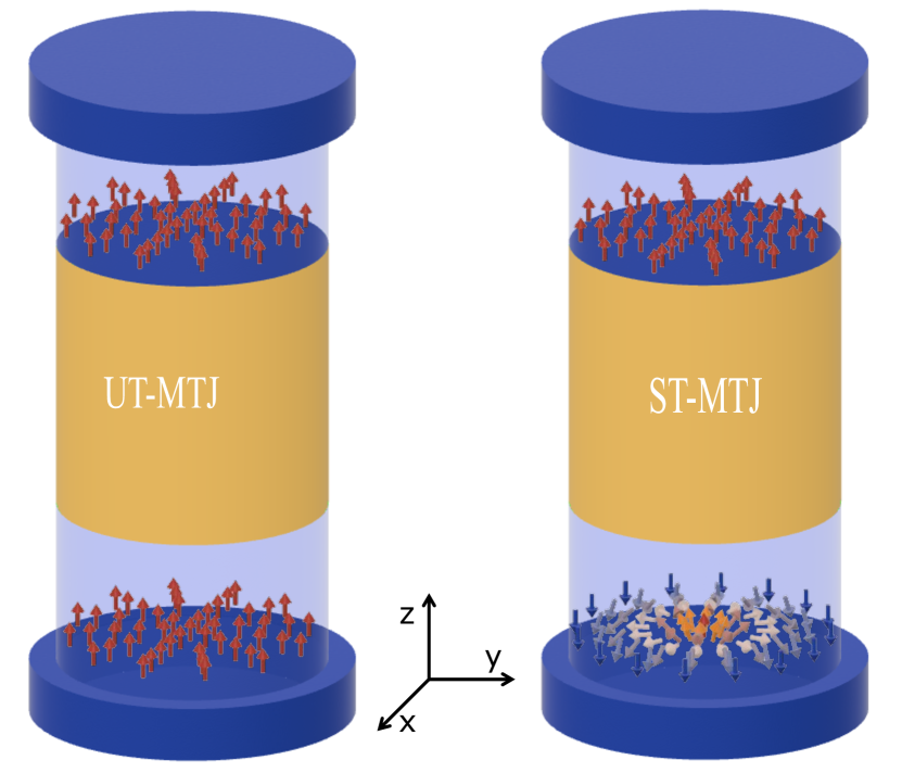
Figure 1: The Schematics of UT-MTJ(on left) and ST-MTJ(on right)

We commence with the Hamiltonian matrix H of the device, the matrix for the energy-resolved, spin-dependent single-particle Green’s function G(E) can be expressed as

$$G(E)=[EI-H-\Sigma]^{-1},$$ (1)

where, the device Hamiltonian matrix ($H=H_{0}+U$) has a spin-dependent tight-binding Hamiltonian term $H_{0}$ and the applied potential profile matrix $U$. The quantity $\Sigma$ represents the spin-dependent self-energy matrix of the bottom and top FM contact, evaluated within the tight-binding framework with open boundary conditions.

We utilized the finite difference tight-binding model for the device Hamiltonian with first nearest neighbor interaction Sharma et al. (2021). The device consists of $N$ lattice points in the direction of transport ($\hat{z}$), which includes the channel/insulator region (N-4 points), with one layer from both the ferromagnetic layers (2 points), and one layer representing the interaction between the ferromagnetic and insulator interface for both the ferromagnetic layers (2 points). Both ferromagnetic contacts have been described using the Stoner model of ferromagnetism with ferromagnetic exchange energy ($\delta$) Ralph and Stiles (2008), effective mass ($m_{FM}^{*}$), and Fermi energy ($E_{f}$). The Hamiltonian ($H_{0}$) can be expressed as a block matrix of order $N\times N$, with each block having dimensions of $P\times P$, where $P=2LM$, $L$ and $M$ are the number of points along the $\hat{x}$ and $\hat{y}$ directions, respectively, and an extra factor of 2 accounts for spin degree of freedom.

$$\left[H_{0}\right]=\left(\begin{array}[]{cccccccc}H_{B}^{FM}&\tau_{B}^{FM}&0&.&.&.&.&.\\ \tau_{B}^{\dagger FM}&H_{I}^{B\rightarrow C}&\tau_{C}&0&.&.&.&.\\ 0&\tau_{C}^{\dagger}&H^{C}&\tau_{C}&0&.&.&.\\ .&0&\tau_{C}^{\dagger}&H^{C}&\tau_{C}&0&.&.\\ .&.&0&.&.&.&0&.\\ .&.&.&0&.&.&.&0\\ .&.&.&.&0&\tau_{C}^{\dagger}&H_{I}^{C\rightarrow T}&\tau_{T}^{FM}\\ &.&.&.&.&0&\tau_{T}^{\dagger FM}&H_{T}^{FM}\end{array}\right)$$ (2)

Here, $H^{FM}_{B}$ and $H^{FM}_{T}$ are onsite energy matrices in the transverse directions ($\hat{x}$ and $\hat{y}$) for the ferromagnetic bottom and top contacts, respectively, and can be written as:

$$H_{B/T}^{FM}=(H_{t}^{FM}+2\operatorname{t_{m}}\textbf{I}_{x}\otimes\textbf{I}_{y})\otimes\textbf{I}_{2}+\Delta_{B/T}$$ (3a)

$$H_{t}^{FM}=H^{FM}_{x}\otimes\textbf{I}_{y}+\textbf{I}_{x}\otimes{H}^{FM}_{y}$$ (3b)

$\textbf{I}_{x}$, $\textbf{I}_{y}$, and $\textbf{I}_{2}$ are identity matrices of order $L\times L$, $M\times M$, and $2\times 2$, respectively. $H_{x/y}$ is the tight-binding Hamiltonian of order $L/M\times L/M$ along the $\hat{x}$/$\hat{y}$ direction, given by:

$$[H^{FM}_{x/y}]_{i,j}=\begin{cases}2t_{m},&i=j,\\ -t_{m},&i=j\pm 1,\\ 0,&\text{ else. }\end{cases}$$ (4)

Where $t_{m}=\frac{\hbar^{2}}{2m_{\text{FM}}^{*}a^{2}}$, $\hbar$ is the reduced Planck constant, $m_{\text{FM}}^{*}$ is the effective mass of the ferromagnetic material, and $a$ is the lattice spacing or discretization step. The spin-dependent exchange energy $\Delta_{B/T}$ of the bottom/top ferromagnetic layer with magnetization texture is given by:

$$\Delta_{B/T}=\delta\dfrac{\textbf{I}_{x}\otimes\textbf{I}_{y}\otimes\textbf{I}_{2}-M_{B/T}}{2}$$ (5)

Where $\delta$ is the ferromagnetic exchange energy, and $M_{B/T}$ is a diagonal matrix of order $P\times P$, describing the spatial variation of the magnetization of the bottom/top contact, given by:

$$[M_{B/T}]^{ij}_{ij}=\hat{m}(x_{i},y_{j},z_{B/T}).\sigma$$ (6)

Where $[{M}T]^{ij}{ij}$ is a $2\times 2$ matrix, $\vec{\sigma}$ represents Pauli’s matrices, and $\hat{m}(x_{i},y_{j},z_{B/T})$ is the spatially varying unit vector of magnetization of the bottom/top ferromagnetic layer. The $\tau^{FM}_{B/T}$ is the spin-dependent coupling matrix of the bottom/top ferromagnetic layer, given by:

$$\tau^{FM}_{B/T}=-t_{m}(\textbf{I}_{x}\otimes\textbf{I}_{y}\otimes\textbf{I}_{2}).$$ (7)

Similarly, $H^{C}$ is the onsite energy matrix in the transverse direction of the channel and is given by:

$$H^{C}=(H_{t}^{C}+2\operatorname{t_{c}}\textbf{I}_{x}\otimes\textbf{I}_{y})\otimes\textbf{I}_{2}$$ (8a)

$$H_{t}^{C}=H^{C}_{x}\otimes\textbf{I}_{y}+\textbf{I}_{x}\otimes{H}^{C}_{y}$$ (8b)

$t_{c}=\frac{\hbar^{2}}{2m_{c}^{*}a^{2}}$ represents the site-to-site hopping energy of the channel with an effective mass $m^{*}_{c}$. The spin-dependent coupling matrix of the channel region is given by:

$$\tau_{C}=-t_{c}(\textbf{I}_{x}\otimes\textbf{I}_{y}\otimes\textbf{I}_{2}).$$ (9)

$H^{B\rightarrow C}_{I}$ and $H^{C\rightarrow T}_{I}$ are the spin-dependent on-site energy matrices of the interface between the channel and the ferromagnetic material, given by:

$$H_{I}^{B\rightarrow C/C\rightarrow T}=\left[H_{t}^{I}+(t_{c}+t_{m})\textbf{I}_{x}\otimes\textbf{I}_{y}\right]\otimes\textbf{I}_{2}$$ (10a)

$$H_{t}^{I}=H^{I}_{x}\otimes\textbf{I}_{y}+\textbf{I}_{x}\otimes{H}^{I}_{y}$$ (10b)

$H^{I}_{x/y}$ is the tight-binding Hamiltonian of order $L/M\times L/M$ along the $\hat{x}$/$\hat{y}$ direction at the interface, given by:

$$[H^{I}_{x/y}]_{i,j}=\begin{cases}t_{m}+t_{c},&i=j,\\ -(t_{m}+t_{c})/2,&i=j\pm 1,\\ 0,&\text{ else. }\end{cases}$$ (11)

The self-energy matrix within the 3D-NEGF framework for the device, with its Hamiltonian defined by Eq. 2, can be articulated as

$$\Sigma_{i,j}=\begin{cases}\Sigma_{B},&i=j=1,\\ \Sigma_{T},&i=j=N,\\ \textbf{0},&\text{ else. }\end{cases}$$ (12)

Here, $\Sigma$ and $\Sigma_{B/T}$ matrices of order $NP\times NP$ and $P\times P$, respectively. The broadening matrices corresponding to both the FMs can be expressed using self energy matrix as

$$\Gamma_{B/T}=i(\Sigma_{B/T}-\Sigma^{\dagger}_{B/T})$$ (13)

The spin and charge current of device can be calculated using transmission operator $T_{op}$ given by

$$\hat{T}_{op}(E)=(\Gamma_{T}\otimes E_{NN})G(\Gamma_{B}\otimes E_{11})G^{\dagger}$$ (14)

where, $E_{11}$ & $E_{NN}$ are the matrix unit, matrices of order $N\times N$.

The charge current and spin current are calculated by integrating the trace of the transmission operator over the energy.

$$I=\frac{q^{2}}{\hbar}\int dE\operatorname{Re}\left[\operatorname{Tr}\left(\hat{T}_{op}\right)\right](f_{T}(E)-f_{B}(E)),$$ (15)

$$I_{S\sigma}=\frac{q^{2}}{\hbar}\int dE\operatorname{Re}\left[\operatorname{Tr}\left(\sigma\cdot\hat{T}_{op}\right)\right](f_{T}(E)-f_{B}(E)),$$ (16)

Where $f_{B}(E)$ and $f_{T}(E)$ are the Fermi–Dirac distributions of the bottom/free ferromagnetic (FM) and top/fixed FM contacts, respectively.

II.1 Uniform Magnetization and Decoupled Spacio-Eigen Approach of NEGF

We first outline the decoupled spatio-eigen approach of NEGF to address the formidable computational demands of solving large 3D systems such as UT-MTJs. If both the FMs have uniform magnetization, then their exchange energy matrix can be written as:

$$\Delta_{B/T}=\textbf{I}_{x}\otimes\ \textbf{I}_{y}\otimes\left[\delta\left(\dfrac{\textbf{I}_{2}-\hat{m}_{B/T}.\sigma}{2}\right)\right]$$ (17)

$\hat{m}_{B/T}$ is the directions of magnetization of bottom/top contact and $\delta$ is exchange splitting energy. In the case of uniform magnetization, the Hamiltonian in transverse direction $H^{FM}_{B}$ & $H^{FM}_{T}$ (see Eq. 3) can be simultaneously block-diagonalized up to spin-dependent block. The Hamiltonian components independent of the spin-splitting terms $H_{t}^{FM}$, $H^{C}_{t}$, and $H^{I}_{t}$ in Eqs.3, 8, and 10 can be simultaneously diagonalized with their eigenvalues denoted as $\epsilon^{FM}_{i}$, $\epsilon^{C}_{i}$, and $\epsilon^{I}_{i}$, respectively.

Figure 2: Transformation of UT-MTJ from real space basis to spatio-eigen basis

The off-diagonal elements in the tight-binding Hamiltonian (Eq. 4) along the transverse directions represent connections between two lattice points in the transverse direction. Through the simultaneous diagonalization of the transverse Hamiltonian matrices, i.e., $H_{t}^{FM}$, $H_{t}^{C}$, $H_{t}^{I}$, our device (UT-MTJ) is effectively partitioned into multiple decoupled spin-dependent 1-D channels, each corresponding to different eigenvalues along the transverse direction. This enables us to formulate NEGF equations in a decoupled spatio-eigen basis for each 1-D channel independently(2).

In this context, the Hamiltonian for each of these eigenmodes ($i$) is represented by:

$$\left[H^{i}_{0}\right]=\left(\begin{array}[]{cccccccc}\alpha_{B}^{FM}&\beta_{B}^{FM}&0&.&.&.&.&.\\ \beta_{B}^{\dagger FM}&\alpha_{I}^{B\rightarrow C}&\beta_{C}&0&.&.&.&.\\ 0&\beta_{C}^{\dagger}&\alpha_{C}&\beta_{C}&0&.&.&.\\ .&0&\beta_{C}^{\dagger}&\alpha_{C}&\beta_{C}&0&.&.\\ .&.&0&.&.&.&0&.\\ .&.&.&0&.&.&.&0\\ .&.&.&.&0&\beta_{C}^{\dagger}&\alpha_{I}^{C\rightarrow T}&\beta_{T}^{FM}\\ &.&.&.&.&0&\beta_{T}^{\dagger FM}&\alpha_{T}^{FM}\end{array}\right)$$ (18)

where $\alpha_{B}^{FM}$, $\alpha_{I}^{B\rightarrow C}$, $\alpha^{C}$, $\alpha_{I}^{C\rightarrow T}$, and $\alpha_{T}^{FM}$ are spin-dependent on-site energy matrices of the bottom FM, interface between the bottom FM and the channel region, channel, interface between the channel and the top FM contact, respectively, given by:

$$\alpha_{B/T}^{FM}=\left(2t_{m}+\epsilon_{i}^{FM}\right)\textbf{I}_{2}+\Delta^{2\times 2}_{B/T}$$ (19a)

$$\alpha_{I}^{B\rightarrow C/C\rightarrow T}=\left(t_{c}+t_{m}+\epsilon_{i}^{I}\right)\textbf{I}_{2}$$ (19b)

$$\alpha^{C}=\left(2t_{c}+\epsilon_{i}^{C}\right)\textbf{I}_{2}$$ (19c)

Where the spin-splitting energy matrix for these spatio-eigen modes is given by $\Delta^{2\times 2}_{B/T}=\delta\frac{\textbf{I}_{2}-\hat{m}_{B/T}.\sigma}{2}$, as shown in Eq. 17. The matrices $\beta^{FM}_{B/T}$ and $\beta^{C}$ are the spin-dependent coupling matrices of the bottom/top FM contact and channel, respectively, given by:

$$\beta^{FM}_{B/T}=-t_{m}\textbf{I}_{2}$$ (20a)

$$\beta^{C}=-t_{c}\textbf{I}_{2}.$$ (20b)

Now, this recasting of the Hamiltonian ($H_{0}$) allows one to solve NEGF for each eigen ($i$) 1D-channel independently. The non-equilibrium Green’s function of each channel ($i$) can be written as:

$$[G^{i}(E)]=[E\textbf{I}-(H^{i}_{0}+U)-\Sigma^{i}]^{-1},$$ (21)

where, the self energy matrix $\Sigma^{i}$ sigma is give by

$$\Sigma_{mn}^{i}=\begin{cases}\Sigma_{B}^{i},&m=n=1,\\ \Sigma_{T}^{i},&m=n=N,\\ 0_{2,2},&\text{ else. }\end{cases}$$ (22)

Assuming the reflection-less contact with an open-boundary condition, each term of the self-energy can be written as:

$$\Sigma_{B/T}^{i}=-t_{m}R_{B/T}\left[\begin{array}[]{cc}\exp\left(ik_{B/T}^{\uparrow,i}a\right)&0\\ 0&\exp\left(ik_{B/T}^{\downarrow,i}a\right)\end{array}\right]R_{B/T}^{\dagger}$$ (23)

where $R_{B/T}$ is a spinor rotation matrix that rotates self-energy matrices from $\hat{z}$ to along the direction of magnetization of the bottom/top contactf. The $k_{B/T}^{\uparrow/\downarrow,i}$ are related to the spin-dependent $E-k$ relation inside the FM as:

$$E=\epsilon^{FM}_{i}+u_{B/T}+2t_{m}\left(1-\cos k_{B/T}^{\uparrow,i}a\right),$$ (24a)

$$E=\epsilon^{FM}_{i}+\delta+u_{B/T}+2t_{m}\left(1-\cos k_{B/T}^{\downarrow,i}a\right)$$ (24b)

Where $u_{B/T}$ is the potential at the bottom/top contact. The charge and spin current can be calculated by adding the current of each individual mode as:

$$I=\frac{q^{2}}{\hbar}\int dE\sum_{i}\operatorname{Re}\left[\operatorname{Tr}\left(\hat{T}^{i}_{op}\right)\right](f_{T}(E)-f_{B}(E)),$$ (25)

The major computational advantage of the spatio-eigen approach emerges from the fact that we need not solve NEGF for all eigen (i) 1D-channels to capture current. It can be deduced from Eq. 24 that for a specific energy (E), if:

$$\lvert 1-\frac{E-\delta-\epsilon^{FM}_{i}-u_{B/T}}{2t_{m}}\rvert>1$$ (26)

Then, $k_{B/T}^{\uparrow/\downarrow,i}$ becomes purely imaginary, resulting in the reduction of $[\Gamma^{i}_{T}]$ and $[\Gamma^{i}_{B}]$ to zero. It leads to the disappearance of current flow (Eq. 25) from the contact to the channel. Consequently, the higher eigen ($i$) 1D-channel does not contribute to the current flow, allowing for the restriction of any NEGF calculation beyond a certain eigenvalue.
The decrease in current at higher eigen-energy levels can be explained by the eigenvalues associated with specific eigenbasis/mode represent the electron’s energy in the transverse direction. As a result, when the transverse energy exceeds E, the contribution to the current from each mode rapidly diminishes. This understanding drives the development of a more efficient approach, focusing exclusively on contributions from lower energy levels to enhance computational efficiency.

II.2 Micromagnetic Texture and Coupled Spacio-Eigen Approach of NEGF

The NEGF’s decoupled spacio-eigen approach encounter difficulties in cases involving an MTJ with ferromagnetic contacts featuring micromagnetic textures, like magnetic skyrmions etc Gobel et al. (2021) . The challenge arises because the transverse Hamiltonian of the contacts, denoted as $H^{FM}_{B}$ and $H^{FM}_{T}$, can no longer be block-diagonalized simultaneously to a smaller order matrix (see Eq.3). This results in the breakdown of the decoupled spatio-eigen approach of NEGF. However, the central argument from the above section—namely, the vanishing contribution of higher modes in current—can still be leveraged for the efficient NEGF calculation of MTJs with non-uniform magnetization textures. It can be noted that the earlier effort to combine quantum transport with micromagnetism by P. Flauger et al.Flauger et al. (2022), overlooked the simultaneous diagonalization of the transverse Hamiltonian. This oversight limits the applicability of their formalism to large micromagnetic structures at best. Whereas, the methodology described in this section can be applied to any transverse Hamiltonian of the contacts that does not preserve translational symmetry in the transverse directions. The spin/charge current is calculated by taking the trace of the transmission matrix, hence the part of transmission operator which is involved in the trace (see Eq. 13 & 14), reduces to

$$T_{\text{op }}\\ (E)=\left(\Gamma_{T}\right)\left(G_{N,1}\right)\left(\Gamma_{B}\right)\left(G_{N,1}^{\dagger}\right)$$ (27)

Here, $G_{N,1}$ represents the element (a sub-matrix of order $P\times P$) at the Nth row (last row) and 1st column of the NEGF’s matrix. Note that the transverse Hamiltonian for the bottom ($H_{B}^{FM}$) and top ($H_{T}^{FM}$) contacts are not simultaneously diagonalizable. However, the transverse Hamiltonian of the channel ($H^{C}$) and the top contact ($H_{T}^{FM}$) can be simultaneously diagonalized. In the coupled spatio-eigen approach of NEGF, we choose the simultaneous eigen vectors of $H_{T}^{FM}$ & $H^{C}$ as the transverse eigen-basis ($|\epsilon_{i}\rangle$) to re-caste the device (contacts+channel) transverse Hamiltonians and the coupling matrices (see Eqs. 7 & 9). In the transverse eigen-basis, $H_{T}^{FM}$ and $H^{C}$ are transformed to their respective eigen matrices $\epsilon^{FM}_{T}$ and $\epsilon^{C}$, while the coupling matrices remain intact. Whereas, the non-commutative nature between the transverse Hamiltonians of the bottom contact ($H_{B}^{FM}$) and the top contact ($H_{T}^{FM}$) results in $H_{B}^{FM}$ transformation to a non-diagonal matrix in the transverse eigen-basis(3.

$$H^{FM}_{B}=\textbf{U}^{\dagger}\epsilon^{FM}_{B}\textbf{U}$$ (28)

$$\textbf{U}_{i,j}=\langle\epsilon^{\prime}_{i}|\epsilon_{j}\rangle$$ (29)

where, $|\epsilon^{\prime}_{i}\rangle$ and $|\epsilon_{i}\rangle$ are the eigen-basis set of the bottom contact and the transverse eigen-basis set, respectively.

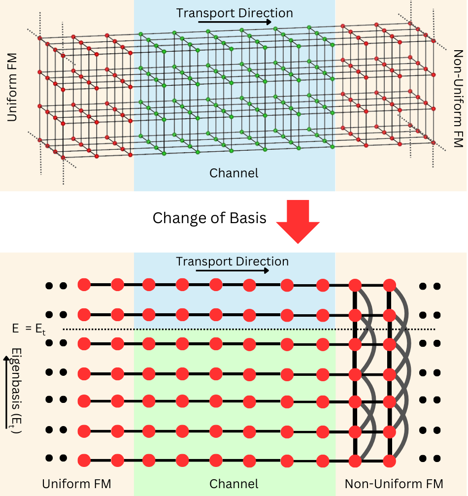
Figure 3: Transformation of ST-MTJ from real space basis to spatio-eigen basis

Since the coupling matrices remain intact in the trasverse eigen-basis, the device in the spacio-eigen approach of NEGF can be envision as shown in the Fig. 3. The self-energy matrix for the top contact in the transverse eigen-basis take diagonal form, articulated as

$$\Sigma_{T(i,j)}=\begin{cases}-t_{m}\exp\left(ik^{i}_{T}a\right),&i=j,\\ 0,&\text{ else. }\end{cases}$$ (30)

$$E=\epsilon^{FM}_{T,i}+u_{T}+2t_{m}\left(1-\cos k^{i}_{T}a\right).$$ (31)

Here, $\epsilon^{FM}_{T,i}$ represents the transverse eigenvalue of the top contact. The broadening matrix $[\Gamma_{T}]{i,i}=[\Sigma_{T}]{i,i}-[\Sigma^{\dagger}{T}]_{i,i}$ also takes on a diagonal form. In the context of a decoupled scenario, In the context of a decoupled scenario, it is observed that the expression $e^{ik_{T}a}$ transforms into a fully real value beyond a specific transverse eigenvalue. As a result, the associated entries for these transverse energies in the broadening matrix become zero. This leads to two distinct sets of eigenvalues: the ‘relevant’ set, actively contributing to transmission, and the ‘irrelevant’ set, which does not play a role in conduction. Consequently, the transverse eigen matrices of the top FM can be neatly organized into block matrices of size $2\times 2$

$$\begin{array}[]{l}\epsilon^{FM}_{T}=\left(\begin{array}[]{ll}\epsilon^{T}_{rev}&0\\ 0&\epsilon^{T}_{irr}\end{array}\right)\end{array}$$ (32)

In this context, $\epsilon^{T}_{rev}$ encompasses all the eigenvalues of the top contact below a threshold energy, beyond which both $e^{ik_{T}a}$ and $e^{ik_{B}a}$ become purely real. The remaining eigenvalues are included in $\epsilon^{T}_{irr}$. A similar partition is applied to the eigenvalues of the bottom contact. With this separation, the broadening matrix of the top contact is simplified to:

$$\begin{array}[]{l}\Gamma_{T}=\left(\begin{array}[]{ll}\Gamma^{T}_{rel}&0\\ 0&0\end{array}\right)\end{array}$$ (33)

The self-energy matrix for the bottom contact can be obtained by transforming the self-energy ($\Sigma_{B}^{{}^{\prime}}$) to the transverse eigen basis using the unitary transformation as described by the Eq. 29.

$$\Sigma_{B}=\textbf{U}^{\dagger}\Sigma_{B}^{{}^{\prime}}\textbf{U}$$ (34)

where, $\Sigma^{{}^{\prime}}_{B}$ is self energy of the bottom contact in $|\epsilon^{\prime}_{i}\rangle$ eigen basis, given by

$$\Sigma^{{}^{\prime}}_{B(i,j)}=\begin{cases}-t_{m}\exp\left(ik^{i}_{B}a\right),&i=j,\\ 0,&\text{ else. }\end{cases}$$ (35)

$$E=\epsilon^{FM}_{B,i}+u_{B}+2t_{m}\left(1-\cos k^{i}_{B}a\right).$$ (36)

where, $\epsilon^{FM}_{B,i}$ is transverse eigen value of the bottom contact. Employing the same rationale as presented in the equation in Eig. 33, the broadening matrix of the bottom contact in the traverse eigen-basis can be written as

$$\begin{array}[]{l}\Gamma_{B}=\textbf{U}^{\dagger}\left(\begin{array}[]{ll}\Gamma^{{}^{\prime}B}_{rev}&0\\ 0&0\end{array}\right)\textbf{U}.\end{array}$$ (37)

If we partition the matrix U into block matrices akin to $\Gamma$ and $\Sigma$, the aforementioned equation can be expressed as

$$\begin{array}[]{l}\Gamma_{B}=\left(\begin{array}[]{cc}U_{11}^{+}&U_{21}^{+}\\ U_{12}^{+}&U_{22}^{+}\end{array}\right)\left(\begin{array}[]{ll}\Gamma^{{}^{\prime}B}_{rel}&0\\ 0&0\end{array}\right)\left(\begin{array}[]{ll}U_{11}&U_{12}\\ U_{21}&U_{22}\end{array}\right)\\ \end{array}$$ (38)

which, simplifies to

$$\begin{array}[]{l}\Gamma_{B}=\left(\begin{array}[]{ll}\Gamma_{11}&\Gamma_{12}\\ \Gamma_{21}&\Gamma_{22}\end{array}\right)\end{array}$$ (39)

Similarly, the matrix $G_{N,1}$ can be represented in a $2\times 2$ block matrix as

$$\begin{array}[]{l}G_{N,1}=\left(\begin{array}[]{ll}g_{11}&g_{21}\\ g_{12}&g_{22}\end{array}\right).\end{array}$$ (40)

Using Eq. 33, 39 & 40, the transmission in Eq. 27 can be written as

$$T_{\text{op }}(E)=\left(\Gamma^{T}_{rel}\right)\left(g_{11}\right)\left(\Gamma_{11}\right)\left(g_{11}^{\dagger}\right)+$$ (41)

$$\left(\Gamma^{T}_{rel}\right)\left(g_{12}\right)\left(\Gamma_{21}\right)\left(g_{11}^{\dagger}\right)+\left(\Gamma^{T}_{rel}\right)\left(g_{11}\right)\left(\Gamma_{11}\right)\left(g_{12}^{\dagger}\right)+$$

$$\left(\Gamma^{T}_{rel}\right)\left(g_{12}\right)\left(\Gamma_{21}\right)\left(g_{12}^{\dagger}\right)$$

The entries of unitary transformation U from bottom contact to transverse eigen basis described by Eq. 29, represent the overlap of the eigenbases of the bottom and top contacts. Thus, we expect that eigenbases with similar wavelengths will exhibit higher overlap. As we move to lower/higher transverse energy eigenvectors (while keeping one eigenvalue constant in Eq. 29), we should observe a decrease in overlap. This decrease corresponds to the decrease/increase in wavelength for a given eigenvector. We expect U to feature a region of high overlap near the diagonal (as the eigenvalues of both contacts are of the same order). Therefore, if we further divide $U_{12}$ and $U_{21}$ in block of $2\times 2$ matrices, they are expected to have the following form

$$U_{12}=\left(\begin{array}[]{ll}0&0\\ u&0\end{array}\right)\\$$ (42a)

$$U_{21}=\left(\begin{array}[]{ll}0&u^{\dagger}\\ 0&0\end{array}\right)\\$$ (42b)

The equation suggests that the primary overlap occurs between the higher energy eigenvectors of the relevant set and the lower energy eigenvectors of the irrelevant set. This overlap can result in minor conduction within the irrelevant set. To mitigate this effect, we can ensure that certain additional relevant eigenvectors, which overlap with the irrelevant set, do not contribute to conduction themselves. This can be achieved by increasing the threshold for relevant eigenvalues. As a result, specific diagonal entries of the relevant broadening matrix $\Gamma^{B/T}{rev}$ are set to zero. This condition can be expressed as follows:

$$\begin{array}[]{l}\Gamma^{{}^{\prime}B/T}_{rev}=\left(\begin{array}[]{ll}\Gamma&0\\ 0&0\end{array}\right).\end{array}$$ (43)

Here, $\Gamma^{{}^{\prime}B/T}_{rev}$ is also partitioned into block matrices, similar to $U_{12}$ and $U_{21}$ for the sake of clarity. Now, if we substitute the expressions from Eq. 43 and Eq. 42 into Eq. 39, it simplifies to:

$$\begin{array}[]{l}\Gamma_{B}=\left(\begin{array}[]{ll}\Gamma_{11}&0\\ 0&0\end{array}\right)\end{array}$$ (44a)

$$\Gamma_{11}=\textbf{U}_{11}^{\dagger}\Gamma^{B}_{rel}\textbf{U}_{11}$$ (44b)

Hence, the contributing expression of transmission is reduced to:

$$T_{\text{op }}(E)=\left(\Gamma^{T}_{rel}\right)\left(g_{11}\right)\left(\Gamma_{11}\right)\left(g_{11}^{\dagger}\right).$$ (45)

We can obtain the expression for $g_{11}$ in spacio-eigen approach of NEGF using Eq. 1. We re-caste device Hamiltonian in spatio-eigen basis i.e transverse Hamiltonians and coupling matrices being in the simultaneous transverse eigen-basis of the top contact & channel. The inverse of the Green function can be represented as a $2\times 2$ block matrix.

$$\begin{array}[]{l}E\textbf{I}-H-\Sigma=\left(\begin{array}[]{ll}A&B\\ C&D\end{array}\right)\end{array}$$ (46)

$$A=E\textbf{I}-H^{FM}_{B}-\Sigma^{\prime}_{B}$$ (47a)

$$B=[t_{m}\textbf{I}\ \textbf{0}\ \textbf{.}\ \textbf{.}\ \textbf{.}\ \textbf{0}]$$ (47b)

$$C=B^{\dagger}$$ (47c)

Where, $D$ represents the rest of the matrix, which can be viewed as a block matrix of dimensions $N-1\times N-1$, with each block having a dimension of $P\times P$, consistent with matrix A. Then, the matrix $G_{1N}$ simplifies to (refer to the Appendices):

$$G_{1N}=-t_{m}(D_{N-1,1}^{-1})(A-t_{m}^{2}(D_{1,1})^{-1})^{-1}$$ (48)

As all blocks of $D$ are diagonal matrices, both $(D^{-1})_{11}$ and $(D^{-1})_{N-1,1}$ are also diagonal matrices. Therefore, these matrices, along with matrices A, will be expressed in terms of relevant and irrelevant blocks as::

$$\begin{array}[]{l}A=\left(\begin{array}[]{ll}a_{11}&a_{21}\\ a_{12}&a_{22}\end{array}\right)\end{array}$$ (49a)

$$\begin{array}[]{l}D_{1,1}^{-1}=\left(\begin{array}[]{ll}d_{1}&0\\ 0&d_{2}\end{array}\right)\end{array}$$ (49b)

$$\begin{array}[]{l}D_{N-1,1}^{-1}=\left(\begin{array}[]{ll}e_{1}&0\\ 0&e_{2}\end{array}\right)\end{array}$$ (49c)

Since we are interested in $g_{11}$ (see Eq. 40), we can expand the $G_{N,1}$ matrix into $2\times 2$ blocks and replace A, $(D^{-1})_{11}$, and $(D^{-1})_{N-1,1}$ using Eq. 49. This allows us to obtain $g_{11}$ using the inverse of a $2\times 2$ block matrix (refer to the Appendix).

$$g_{11}=-t_{m}(e_{1})(a_{11}-t_{m}^{2}d_{1}-a_{12}(a_{22}-d_{2})a_{21})^{-1}$$ (50)

Expanding the expressions of $a$’s using Eq. 47.a, we obtain:

$$g_{11}=-t_{m}(e_{1})(U^{\dagger}_{11}(E\textbf{I}-\epsilon^{T}_{B}-\Gamma^{B}_{rel})U_{11}-\tau_{m}^{2}d_{1}+O(u^{2}))^{-1}$$ (51)

As evident from the analysis, the formula for $g_{11}$ (and consequently, the transmission expression) has been simplified to matrices associated only with relevant eigenvalues. However, a factor contingent on the order of squares and beyond, dependent on matrix $u$, remains. As previously explained, matrix $u$ characterizes the coupling between the higher relevant eigenbasis and the lower irrelevant basis. This factor diminishes as we elevate the relevance threshold, thereby minimizing its impact. Consequently, the transmission expression can be constructed solely from the relevant terms with appropriate eigen threshold. The spacio-eigen framework of the NEGF, presented, eliminates the necessity of solving the 3D NEGF, while preserving the system’s physics under non-equilibrium conditions. The substantial reduction in computational requirements stems from the ability to fully construct the transmission operator using a set of ‘relevant’ transverse eigen states of the system. It is noteworthy that the spacio-eigen framework of the NEGF is generic and capable of handling translationally ‘variant’ system provided that the system’s Hamiltonian can be derived from the tensor sum of Hamiltonian (see Eq. 3).

III Modelling

We utilized the method presented above to model a Magnetic Tunnel Junction (MTJ) with one of its contacts containing a skyrmion. Our focus in this paper is on Bloch-type and Néel-type skyrmions. For the majority of simulations, the diameter of the MTJ is set to 20 nm, and the width of the channel is 1 nm. The diameter of the skyrmion in the MTJ is considered to be 10 nm. During the scaling of the MTJ, we assumed that the size of the skyrmion also shrinks proportionally, which may be achieved using a higher DMI interaction Sampaio et al. (2013). The effective mass of electrons in the channel and ferromagnet is 0.8 $m_{e}$ and 0.18 $m_{e}$, respectively. The Fermi energy of the system is set at 2.25 eV, and the exchange splitting is determined to be 2.15 eV Salahuddin and Datta (2006).

IV Results and discussion

We commence our analysis by examining the current-voltage characteristics of the MTJ with skyrmion texture (ST-MTJ) in different relative orientations of skyrmion core and the uniform ferromagnetic (UFM) layer (see Fig. 1). We also sketch a comparison of the ST-MTJ and the UMT-MTJ. n Fig.4(a), we present the current-voltage (IV) characteristics of the ST-MTJ with Bloch-type and Néel-type skyrmions in the parallel (PC) and anti-parallel (APC) configurations. The PC and APC configurations correspond to the relative parallel and anti-parallel orientation of the magnetization of the UFM layer to the core of the magnetic skyrmion, respectively. The I-V characteristics of the Bloch and Néel-type skyrmion in ST-MTJ concur due to the same azimuthal projection of the magnetic texture in the PC and APC. The higher current in the APC in comparison to the PC is caused by greater positive projection of the skyrmion texture on the UFM of the ST-MTJ. The spin texture dependent tunneling in the ST-MTJ lead to higher resistance in the PC and lower resistance in the APC of the device as characterised by the tunnel magnetoresistance (TMR):

$$TMR=\frac{R_{P}-R_{AP}}{R_{AP}}\times 100$$ (52)

here $R_{P}$ and $R_{AP}$ are the resistances in the PC and APC, respectively. It may be noted that for UT-MTJ $TMR=(R_{AP}-R_{P})100/R_{P}$ as resistance is higher in APC than PC. We show in Fig.4(b) the TMR of the ST-MTJ and the UMT-MTJ. It can be inferred from Fig.4(b) that the zero-voltage TMR is approximately 70%, which is notably less than half of the TMR offered by the UMT-MTJ. The reduction in the TMR in the ST-MTJ is associated with spin texture-dependent tunneling, which offers alternate eigen channels for conduction in the APC.

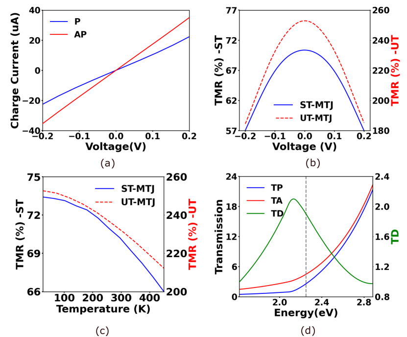
Figure 4: (a) Current-Voltage characteristics in the PC and APC, (b) TMR variation with voltage, (c) TMR roll-off with temperature for both the ST-MTJ and UMT-MTJ devices. (d) Transmission of the ST-MTJ in the PC (TP) and the APC (TA) along with transmission difference (TD=TP-TA)

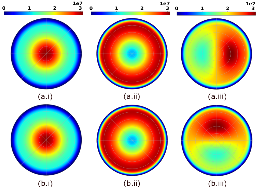
Figure 5: Charge current density($A/m^{2}$) profiles of the ST-MTJ with the UFM oriented (i) parallel, (ii) antiparallel and (iii) orthogonal to the core of the Skyrmion for (a)Néel-type and (b)Bloch-type skyrmion, at 10 mV.

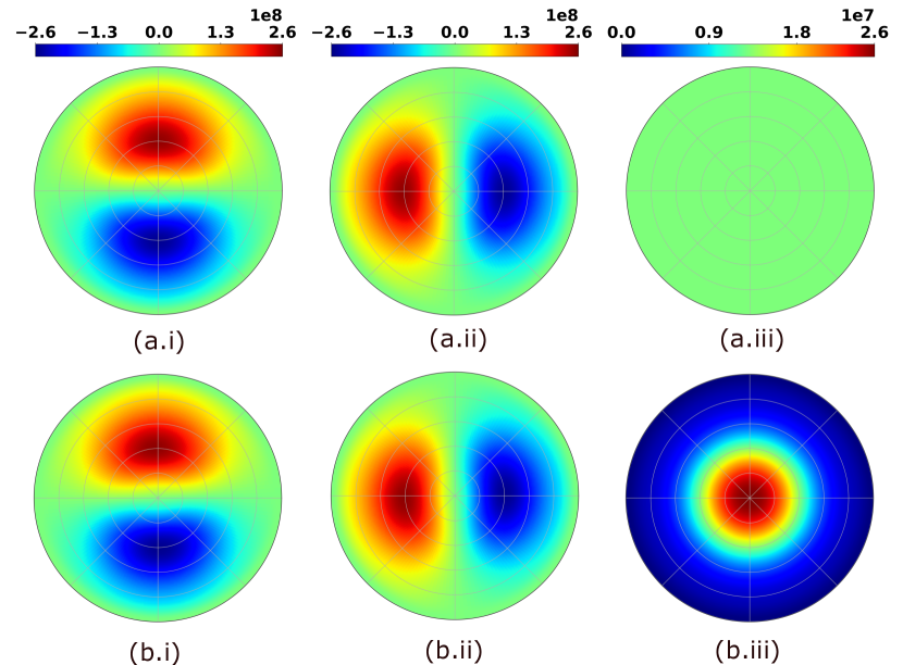
Figure 6: Spin current density($A/m^{2}$) (i) $I_{x}$, (ii) $I_{y}$, (iii) $I_{z}$ at (a)zero volt bias ,and at (b)10mV bias for Néel-type Skyrmion based MTJ

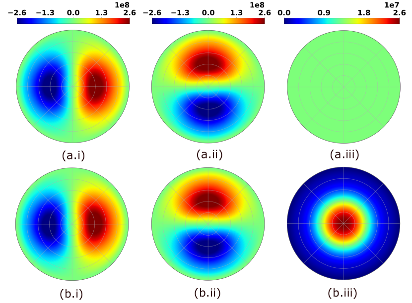
Figure 7: Spin current density($A/m^{2}$) (i) $I_{x}$, (ii) $I_{y}$, (iii) $I_{z}$ at (a)zero volt bias ,and at (b)10mV bias for Bloch-type Skyrmion based MTJ.

We show in the Fig.4(c) a monotonic reduction in the TMR with temperature for both the ST-MTJ and UMT-MTJ devices. The percentage reduction in the TMR with temperature is lower in the ST-MTJ ($\approx$ 11%) than in the UMT-MTJ ($\approx$ 19%). We also note that earlier works Chakraborti and Sharma (2023); Zhao et al. (2022); Kou et al. (2006), have associated the TMR roll-off with temperature to magnon scattering in the UMT-MTJ, but it can be explained without invoking magnon scattering to the first order. To comprehend the TMR roll-off in the ST-MTJ, we refer to Fig.4(d), which illustrates the transmission characteristics at different energy levels for both the PC ($T_{P}$) and APC ($T_{AP}$), along with the transmission difference ($TD=T_{AP}-T_{P}$). It can be seen that the transmission corresponding to the PC is lower than that of the APC for the energy spectra. The difference between transmission ($TD$) increases till $2.13eV$ and subsequently starts to roll off, as the transmission for the PC begins to rise at a faster rate compared to the APC. At very low temperatures, only a narrow range of transmission spectra contributes to current conduction around the Fermi window ($2.25eV$). The broadening of the Fermi window at higher temperatures allows a wide range of transmission spectra to participate in current conduction. The TMR in terms of transmission coefficient can be expressed as:

$$TMR=\frac{\int{T_{D}(E)}(f_{L}-f_{R})dE}{\int T_{P}(E)(f_{L}-f_{R})dE}\times 100$$ (53)

Initially, with an increase in temperature, the contribution to the numerator of Eq. 53 remains almost constant, as the Fermi window below/above the Fermi energy engulfs an increasing/decreasing $T_{D}(E)$, resulting in a slow roll-off in the TMR. However, as the transmission spectra difference ($T_{D}(E)$) below $2.13eV$ begins to contribute at higher temperatures due to a broader Fermi window, the additional transmission contribution from each energy level starts to decrease with temperature, leading to a more pronounced roll-off effect at higher temperatures.

The characteristics of current and current density are also influenced by the orientation of the UFM. The current density depends on the azimuthal projection of the Skyrmion texture on the UFM. In the PC, the current density is highest at the center (approximately $3\times 10^{7}A/m^{2}$) and gradually decreases to zero as we move radially outward. Conversely, in APC, the current at the center reduces significantly (approximately $0.7\times 10^{7}A/m^{2}$), and it increases as we move radially outward, reaching a maximum of approximately ($3\times 10^{7}A/m^{2}$), before declining to zero at the edges. It can be seen that the proposed coupled spacio-eigen approach of NEGF inherently accounts for the vanishing current at the boundary of the device, which can significantly impact the current characteristics as the size of the ST-MTJ reduces. Both in the PC and APC of the skyrmion and UFM, a circular symmetry emerges in the charge current density distribution. It can be associated with the inherent circular symmetry of both the skyrmion and the uniform ferromagnetic layer. However, when the magnetization of UFM is not co-linear to the core of the Skyrmion, the circular symmetry in the current density profile vanishes, as illustrated in Fig. 5(c) and 5(d) for Néel-type Skyrmion and Bloch-type respectively.

In Figures 5(a) and 5(b), the current density is shown for Néel-type and Bloch-type skyrmions, respectively. It’s noticeable that in the anti-parallel (AP) and anti-parallel configuration (APC), the charge density remains consistent between Néel-type and Bloch-type skyrmions. However, in other configurations, such as the perpendicular configuration, they demonstrate differences, as illustrated in Figures 5(a.iii) and (b.iii). Therefore, distinguishing between Néel-type and Bloch-type skyrmions can be achieved through local measurements of the current.

Figure 8: Spin current($A/m^{2}$) $I_{x}$ emerged from UFM when free layer have (a) Néel-type skyrmions (b) Right Handed Bloch-Type skyrmion (c) Left Handed Bloch type skyrmion at a bias of i)-0.1V, ii) 0V and iii) 0.1V

In Figures 6 and 7, we illustrate the spin current profiles for ST-MTJs with Néel and Bloch type skyrmions, respectively, in the parallel configuration at 0 V and 10 mV. The spin current emerging from the uniform ferromagnetic (UFM) layer in ST-MTJs exhibits a textured profile. Figures 6(a.i,a.ii) and 7(a.i,a.ii) demonstrate the emergence of spatially dependent exchange coupling Slonczewski (1989), also known as dissipation-less spin current ($I_{x}$ and $I_{y}$), at zero bias in the ST-MTJs. At non-zero bias, the spin current density along the z-axis ($I_{z}$) is identical for both Néel and Bloch type skyrmions-based ST-MTJs, as shown in Figures 6(b.iii) and 7(b.iii). However, the spin current density $I_{x}$ and $I_{y}$ are rotated by 90 degrees in Néel and Bloch skyrmion-based MTJs, as depicted in Figures 6(b.i,b.ii) and 7(b.i,b.ii). This provides a pathway for Néel and Bloch type skyrmion detection in MTJs through local measurements of exchange coupling.

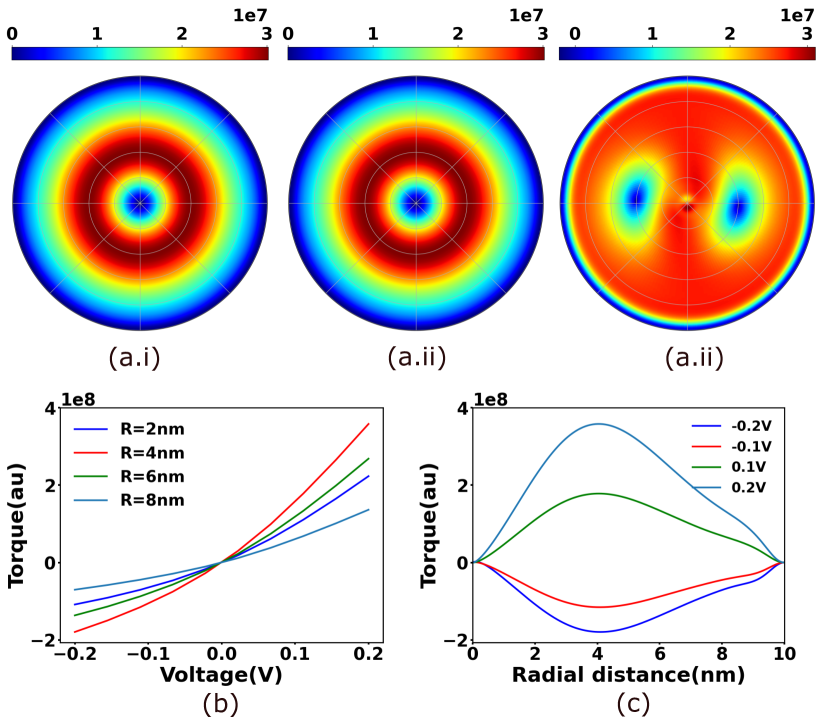
Figure 9: (a)Damping-Like Term(Arb. unit) with Spatial Variation at 20 mV for AC(a.i), APC(a.ii) and orthogonal configuration(a.iii), b)Voltage Dependency at Varying Radial Distances c) Radial Variation at Different Voltages

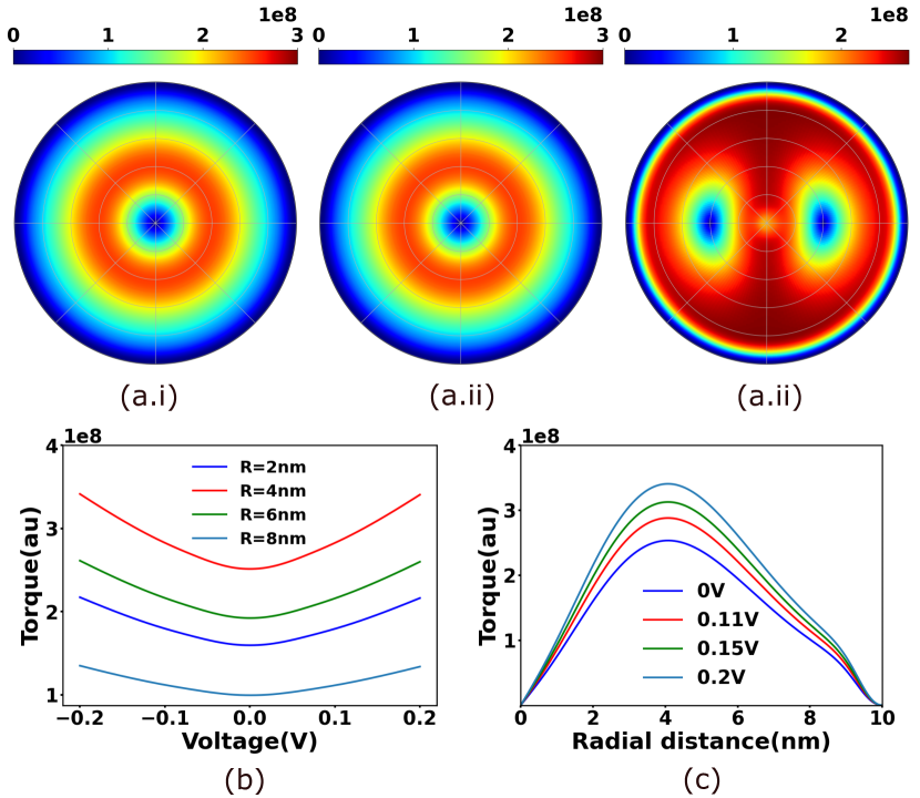
Figure 10: (a)Field-Like Term(Arb. unit) with Spatial Variation at 20 mV for AC(a.i), APC(a.ii) and orthogonal configuration(a.iii), b)Voltage Dependency at Varying Radial Distances c) Radial Variation at Different Voltages

The spin texture emerging from UFM exhibits circular symmetry in the cases of PC and APC, and interesting dynamics can arise under different biasing and Skyrmion types. As depicted in Figure 8, a pattern of rotation emerges as we sweep the voltage from -0.1 to 0.1, and the direction of rotation and phase of the texture can depend on the UMF configuration, micromagnetic texture, etc. Hence, characteristics such as helicity in Bloch-type skyrmions can be determined by carrying out local spin measurements at different voltages.

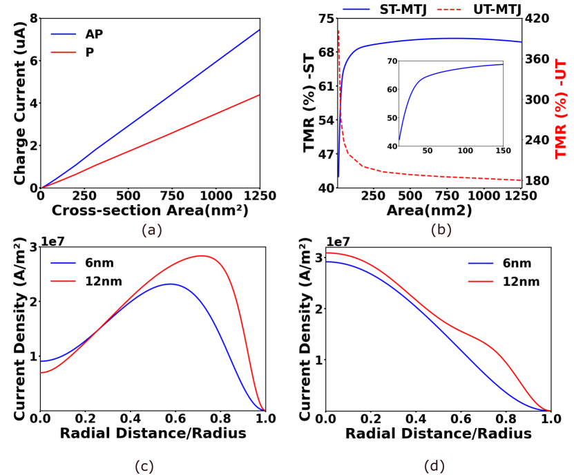
Figure 11: a) Variation of charge current with cross-section area b) Roll-off in TMR with reduction of cross-section area. Radial Variation in charge current for ST-MTJ of diameter 12nm and 6nm for c) APC and d) PC

In this section, we decompose the torque on the skyrmion in the ST-MTJ by using the Landau–Lifshitz–Gilbert–Slonczewski (LLGS) equation described as:

$$\left(1+\alpha^{2}\right)\frac{\partial\hat{m}}{\partial t}= -\gamma\hat{m}\times\left(\vec{H}_{eff}+\vec{h}_{ff}\right)$$ (54)

$$-\gamma\alpha\left(\hat{m}\times\left(\hat{m}\times\left(\vec{H}_{eff}+\vec{h}_{f}\right)\right)\right)$$

$$-\frac{\gamma h}{2qM_{S}V}\left(\left(\hat{m}\times\left(\hat{m}\times\vec{I}_{S}\right)\right)-\alpha\left(\hat{m}\times\vec{I}_{S}\right)\right),$$

where, $\hat{m}(\vec{r})$ is magentization of free layer.

The torque for the dynamics cause by spin current($I_{s}$) is given by

$$\left(1+\alpha^{2}\right)\frac{\partial\hat{m}}{\partial t}= -\frac{\gamma h}{2qM_{S}V}\left(\hat{m}\times\left(\hat{m}\times\vec{I}_{S}\right)\right),$$ (55)

We decompose spin transfer torque components along the unit vector in the direction of $m$, $m\times(m\times M)$, and $m\times M$. The component of torque along the unit vector in the direction of $m\times(m\times M)$ and $m\times M$ are termed as damping/anti-damping/Slonczewski torque ($T_{s}$) and field-like torque ($T_{h}$), respectively.

As depicted in Fig. 9(a) and Fig. 9(b), the $T_{s}$ term indicates that the damping introduced by the UFM in PC exhibits radial variation and circular symmetry. Consequently, different domains within the free layer experience distinct torques. Furthermore, we note that this term exhibits different profiles and values for positive and negative voltages (Fig. 9(c) and Fig. 9(d)), leading to an asymmetrical torque response for these voltage polarities. The bias-dependent torque phenomenon is a well-established concept within the context of UT-MTJs, where the degree of asymmetry has been observed to be contingent upon the angle between ferromagnetic layers Theodonis et al. (2007). In ST-MTJs, the bias-dependent asymmetry varies as a consequence of the distinctive magnetization orientations at different radial distances. We also note a radially varying, circularly symmetric pattern in the field-like term (Fig. 10(a) and Fig. 10(b)). However, unlike the damping/anti-damping terms, this field-like term does not exhibit asymmetry between positive and negative voltages (Fig. 10(d)). These terms play a crucial role in enabling us to comprehensively evaluate the dynamics of micromagnets, which is of utmost significance for their potential applications of ST-MTJ in memory storage and their potential utility as Qubits in topological quantum computers.

Finally, we present the analysis of reduction in the cross-sectional area on the characteristics of the ST-MTJ and UMT-MTJWatanabe et al. (2018); Perrissin et al. (2018). As expected, at larger sizes, the current is found to exhibit a linear relationship with the area (Fig. 11(a)). However, at smaller scales, it deviates from this linear trend, resulting in slightly reduced current. An intriguing observation is that the TMR begins to decrease as we reduce the size of the ST-MTJ (Fig. 11(b)). This reduction becomes pronounced as the device diameter shrinks below 10 nm, suggesting a strong interface at that scale. We can gain insights into this TMR roll-off by examining the current density at 12 nm and 6 nm diameters in the APC (Fig. 11(c)). Firstly, it’s noticeable that the maxima in case of smaller diameter decrease by approximately $\approx 18\%$ as compared to 12 nm ST-MTJ. One trivial explanation could be that boundary effects become more dominant at smaller sizes, leading to a reduction in current density. However, what’s truly intriguing is that the current density at the center actually increases by $\approx 30\%$. This observation implies that at smaller scales, the proximity between regions of higher and lower conduction significantly interferes with their interaction. Their spatial closeness allows the lower conduction pathway to tunnel through alternative routes, thereby enhancing their overall conductance. Consequently, this interference leads to a reduction in the disparity in transmission between the PC and APC configurations, ultimately resulting in a decreased TMR.

V Conclusion

In this work, we introduced computationally efficient spacio-eigen framework of NEGF to abate the requirement of 3D NEGF for system that lack translational invarience and simultaneous eigen-basis along the transverse directions. Using the spacio-eigen approach of NEGF, we delineated the charge/spin characteristics of ST-MTJ with both Bloch and Néel type textures across various voltages, temperatures and sizes. We detailed the appearance of a textured spin current originating from the uniform layer of ST-MTJs and outlined a radially varying, asymmetrical voltage dependence of spin torque. We described the voltage-induced rotation of the spin current texture, coupled with the emergence of helicity in the spin current, especially evident in the case of Néel skyrmions on MTJ under non-equilibrium conditions. We identified the temperature roll-off in the TMR of ST-MTJ and UT-MTJ. We attributed this roll-off to the ballistic transmission spectra abating the need of magnon to the first order. Finally, we described the effect of scaling on ST-MTJ from technological standpoint. Our work presents a computationally manageable approach to integrating micromagnetic and quantum transport, enabling the exploration of a diverse range of topological non-trivial magnetic phases on MTJs. The predicted emergence of a textured spin current holds the potential to induce non-trivial magnetization dynamics, offering diverse fundamental and technological ramifications.

Appendix A Toy Model

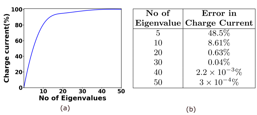
Figure 12: (a) Charge current in the Spatio-Eigen basis (as a percentage of the charge current in the real basis), varying with the number of eigenbases. (b) Error in the charge current in the Spatio-Eigen basis compared to the real basis.

We demonstrate the effectiveness of spacio-eigen approach of NEGF using a toy model of a 2D nanosheet. In our model, we consider a 2D magnetic tunnel junction (MTJ)-like structure, where a 2D insulating channel is positioned between two 2D FM contacts. One contact exhibits uniform magnetization, while the other features a non-uniform texture, where the in-plane angle of magnetization varies according to a Gaussian distribution. In our simulations, we utilize real-space 2D non-equilibrium Green’s function (NEGF) methods to calculate the charge current. Additionally, parallel calculations are conducted using spatio-eigen approch of NEGF method, which employs a smaller set of relevant eigenvalues. As depicted in Fig. 12, we observe that the charge current obtained from using the spacio-eigen approach converges to the charge current obtained from real-space NEGF as the size of the eigenvalue set increases. This comparison provides insights into the accuracy and efficiency of our computational approach.

When the simulation considers 30 eigenvalues, our method yields remarkably accurate results, displaying an error of only 0.04%. The error decreases further to below $3\times 10^{-3}\%$ with just 50 eigenvalues. We also observe an error of less than 0.05% in the spin current for a set of 30 eigenvalue. A similar trend is observed for different device characteristics and non-uniform contacts. Hence, this toy model demonstrates that the argument we presented in the methodology section, regarding the reduction of the effects of conduction and interference from the irrelevant set of eigen states, diminishes as we increase the threshold of the relevant set. The toy model numerically demonstrate that we can capture all the physics of quantum transport using spatio-eigen approaches of NEGF while utilizing only a fraction of computational resources compared to full 3D-NEGF.

Appendix B Inverse of matrix in terms of $2\times 2$ block

If we have a matrix divided into $2\times 2$ matrix, then block wise inverse of such matrix is given by expression

$$\begin{array}[]{l}\left(\begin{array}[]{ll}a&b\\ c&d\end{array}\right)=\left(\begin{array}[]{ll}A&B\\ C&D\end{array}\right)^{-1}\end{array}$$ (56a)

$$a=(A-BD^{-1}C)^{-1}$$ (56b)

$$c=D^{-1}Ca$$ (56c)

$$d=(D-CA^{-1}B)^{-1}$$ (56d)

$$b=A^{-1}Bd$$ (56e)

References

- Gobel et al. (2021) B. Gobel, I. Mertig, and O. A. Tretiakov, Physics Reports 895, 1 (2021).
- Muhlbauer et al. (2009) S. Muhlbauer, B. Binz, F. Jonietz, C. Pfleiderer, A. Rosch, A. Neubauer, R. Georgii, and P. Boni, Science 323, 915 (2009).
- Jonietz et al. (2010) F. Jonietz, S. Mühlbauer, C. Pfleiderer, A. Neubauer, W. Münzer, A. Bauer, T. Adams, R. Georgii, P. Boni, R. A. Duine, K. Everschor, M. Garst, and A. Rosch, Science 330, 1648 (2010).
- Yu et al. (2010) X. Z. Yu, Y. Onose, N. Kanazawa, J. H. Park, J. H. Han, Y. Matsui, N. Nagaosa, and Y. Tokura, Nature 465, 901 (2010).
- Heinze et al. (2011) S. Heinze, K. von Bergmann, M. Menzel, J. Brede, A. Kubetzka, R. Wiesendanger, G. Bihlmayer, and S. Blügel, Nature Physics 7, 713 (2011).
- Hrabec et al. (2017) A. Hrabec, J. Sampaio, M. Belmeguenai, I. Gross, R. Weil, S. M. Chérif, A. Stashkevich, V. Jacques, A. Thiaville, and S. Rohart, Nature Communications 8, 15765 (2017).
- Nagaosa and Tokura (2013) N. Nagaosa and Y. Tokura, Nature Nanotechnology 8, 899 (2013).
- Wang et al. (2018) X. Wang, H. Yuan, and X. Wang, Communications Physics 1, 1 (2018).
- Romming et al. (2013) N. Romming, C. Hanneken, M. Menzel, J. E. Bickel, B. Wolter, K. von Bergmann, A. Kubetzka, and R. Wiesendanger, Science 341, 636 (2013).
- Sampaio et al. (2013) J. Sampaio, V. Cros, S. Rohart, A. Thiaville, and A. Fert, Nature Nanotechnology 8, 839 (2013).
- Garcia-Sanchez et al. (2016) F. Garcia-Sanchez, J. Sampaio, N. Reyren, V. Cros, and J.-V. Kim, New Journal of Physics 18, 075011 (2016).
- Tomasello et al. (2014) R. Tomasello, E. Martinez, R. Zivieri, L. Torres, M. Carpentieri, and G. Finocchio, Sci Rep 4, 6784 (2014).
- Luo et al. (2018) S. Luo, M. Song, X. Li, Y. Zhang, J. Hong, X. Yang, X. Zou, N. Xu, and L. You, Nano Letters 18, 1180 (2018), pMID: 29350935.
- Zhang et al. (2015a) X. Zhang, M. Ezawa, and Y. Zhou, Sci Rep 5, 9400 (2015a).
- Huang et al. (2017) Y. Huang, W. Kang, X. Zhang, Y. Zhou, and W. Zhao, Nanotechnology 28, 08LT02 (2017).
- Bhattacharya et al. (2019) T. Bhattacharya, S. Li, Y. Huang, W. Kang, W. Zhao, and M. Suri, IEEE Access 7, 5034 (2019).
- Zhang et al. (2015b) X. Zhang, Y. Zhou, M. Ezawa, G. P. Zhao, and W. Zhao, Sci Rep 5, 11369 (2015b).
- Psaroudaki and Panagopoulos (2021) C. Psaroudaki and C. Panagopoulos, Phys. Rev. Lett. 127, 067201 (2021).
- Psaroudaki et al. (2023) C. Psaroudaki, E. Peraticos, and C. Panagopoulos, Applied Physics Letters 123, 260501 (2023).
- Xia et al. (2022) J. Xia, X. Zhang, X. Liu, Y. Zhou, and M. Ezawa, Communications Materials 3, 88 (2022).
- Zou et al. (2023) J. Zou, S. Bosco, B. Pal, S. S. P. Parkin, J. Klinovaja, and D. Loss, Phys. Rev. Res. 5, 033166 (2023).
- Penthorn et al. (2019) N. E. Penthorn, X. Hao, Z. Wang, Y. Huai, and H. W. Jiang, Phys. Rev. Lett. 122, 257201 (2019).
- He et al. (2023) B. He, Y. Hu, C. Zhao, J. Wei, J. Zhang, Y. Zhang, C. Cheng, J. Li, Z. Nie, Y. Luo, Y. Zhou, S. Zhang, Z. Zeng, Y. Peng, J. M. D. Coey, X. Han, and G. Yu, Advanced Electronic Materials 9 (2023), 10.1002/aelm.202201240, in press, Article ID: 2201240.
- Li et al. (2022) S. Li, A. Du, Y. Wang, X. Wang, X. Zhang, H. Cheng, W. Cai, S. Lu, K. Cao, B. Pan, N. Lei, W. Kang, J. Liu, A. Fert, Z. Hou, and W. Zhao, Science Bulletin 67, 691 (2022).
- Kasai et al. (2019) S. Kasai, S. Sugimoto, Y. Nakatani, R. Ishikawa, and Y. K. Takahashi, Appl. Phys. Express 12, 083001 (2019).
- Guang et al. (2023) Y. Guang, L. Zhang, J. Zhang, Y. Wang, Y. Zhao, R. Tomasello, S. Zhang, B. He, J. Li, Y. Liu, J. Feng, H. Wei, M. Carpentieri, Z. Hou, J. Liu, Y. Peng, Z. Zeng, G. Finocchio, X. Zhang, J. M. D. Coey, X. Han, and G. Yu, Advanced Electronic Materials 9 (2023), 10.1002/aelm.202200570, in press, Article ID: 2200570.
- Butler et al. (2001) W. H. Butler, X.-G. Zhang, T. C. Schulthess, and J. M. MacLaren, Phys. Rev. B 63, 054416 (2001).
- Slonczewski (1989) J. C. Slonczewski, Phys. Rev. B 39, 6995 (1989).
- Theodonis et al. (2007) I. Theodonis, N. Kioussis, A. Kalitsov, M. Chshiev, and W. Butler, Physical review letters 97, 237205 (2007).
- Gosavi et al. (2017) T. A. Gosavi, S. Manipatruni, S. V. Aradhya, G. E. Rowlands, D. Nikonov, I. A. Young, and S. A. Bhave, IEEE Transactions on Magnetics 53, 1 (2017).
- Sun and Ralph (2008) J. Sun and D. Ralph, Journal of Magnetism and Magnetic Materials 320, 1227 (2008).
- Kim (2012) J. V. Kim, Solid State Physics—Advances in Research and Applications, 1st ed., Vol. 63 (Elsevier Inc., 2012) pp. 217–294.
- Sharma et al. (2017) A. Sharma, A. A. Tulapurkar, and B. Muralidharan, Phys. Rev. Appl. 8, 064014 (2017).
- Kultursay et al. (2013) E. Kultursay, M. Kandemir, A. Sivasubramaniam, and O. Mutlu (2013) p. 256.
- van Dijken and Coey (2005) S. van Dijken and J. M. D. Coey, Applied Physics Letters 87, 022504 (2005).
- Sharma et al. (2016) A. Sharma, A. Tulapurkar, and B. Muralidharan, IEEE Transactions on Electron Devices 63, 4527 (2016).
- Datta (1997) S. Datta, Electronic Transport in Mesoscopic Systems (Cambridge University Press, 1997).
- Slonczewski (1996) J. Slonczewski, Journal of Magnetism and Magnetic Materials 159, L1 (1996).
- Salahuddin and Datta (2006) S. Salahuddin and S. Datta, Applied Physics Letters 89, 153504 (2006).
- Papior et al. (2017) N. Papior, N. Lorente, T. Frederiksen, A. García, and M. Brandbyge, Computer Physics Communications 212, 8 (2017).
- Ashcroft and Mermin (1976) N. W. Ashcroft and N. D. Mermin, Solid State Physics (Holt-Saunders, 1976).
- Sharma et al. (2021) A. Sharma, A. A. Tulapurkar, and B. Muralidharan, Journal of Applied Physics 129, 233901 (2021).
- Ralph and Stiles (2008) D. Ralph and M. Stiles, Journal of Magnetism and Magnetic Materials 320, 1190 (2008).
- Flauger et al. (2022) P. Flauger, C. Abert, and D. Suess, Phys. Rev. B 105, 134407 (2022).
- Chakraborti and Sharma (2023) S. Chakraborti and A. Sharma, Nanotechnology 34, 185206 (2023).
- Zhao et al. (2022) D. Zhao, Y. Wang, J. Shao, Y. Chen, Z. Fu, Q. Xia, S. Wang, X. Li, G. Dong, M. Zhou, and D. Zhu, AIP Advances 12, 055114 (2022).
- Kou et al. (2006) X. Kou, J. Schmalhorst, A. Thomas, and G. Reiss, Applied Physics Letters 88, 212115 (2006).
- Watanabe et al. (2018) K. Watanabe, B. Jinnai, S. Fukami, H. Sato, and H. Ohno, Nature Communications 9, 663 (2018).
- Perrissin et al. (2018) N. Perrissin, S. Lequeux, N. Strelkov, L. Vila, L. Buda-Prejbeanu, S. Auffret, R. Sousa, I. Prejbeanu, and B. Dieny, in 2018 International Conference on IC Design & Technology (ICICDT) (2018) pp. 125–128.