Calibration-Based ALE Model Order Reduction for Hyperbolic Problems with Self-Similar Travelling Discontinuities

Abstract

We propose a novel Model Order Reduction framework that is able to handle solutions of hyperbolic problems characterized by multiple travelling discontinuities. By means of an optimization based approach, we introduce suitable calibration maps that allow us to transform the original solution manifold into a lower dimensional one. The optimization process does not require the knowledge of the discontinuities location. In the online phase, the coefficients of the projection of the reduced order solution onto the reduced space are recovered by means of an Artificial Neural Network. To validate the methodology, we present numerical results for the $1$D Sod shock tube problem and for the $2$D double Mach reflection problem, also in the parametric case.

65M08,35L60,35L67,76L05

1 Introduction

The goal of MOR techniques [6, 15, 14], which are particularly suited for the real-time computations and many-query context, is to obtain efficient and reliable approximations of solutions of high dimensional systems of partial differential equations (PDEs). Let us consider the approximate solution $u(t;\mu)\in L^{2}(\Omega)$ of a parametrized PDE, with $\Omega\subset\mathbb{R}^{d}$, with the parameter $\mu\in\mathcal{P}_{\text{phys}}\subset\mathbb{R}^{s}$ and with time $t\in[0,t_{f}]$: for the spatial discretization one can consider, for instance, the Finite Volume (FV) discretization. We introduce the solution manifold related to this parametric PDE: $\mathcal{M}=\{u(t;\mu)\in V_{\mathcal{N}},\text{ }\mu\in{\mathcal{P}_{\text{phys}}},\text{ }t\in[0,t_{f}]\},$ where $V_{\mathcal{N}}$ is a suitable functional space defined by the chosen spatial discretization. The key idea behind MOR is to represent $\mathcal{M}$ with a finite dimensional linear space $V_{N}$, such that $N\ll\mathcal{N}$, where $N=\text{dim}V_{N}$ and $\mathcal{N}=\text{dim}V_{\mathcal{N}}$. To find the lower dimensional space $V_{N}$, one can use the well known Proper Orthogonal Decomposition (POD) strategy that, given in input a set of discrete solutions (obtained, for example, with the FV method), is able to extract a set of small cardinality $N$, which contains the so-called reduced basis functions that best approximate the manifold. A pivotal aspect for the efficiency of the MOR is the ability of the POD of compressing the discrete solution manifold $\mathcal{M}$: this concept is strictly related to the definition of Kolmogorov $N$-width of $\mathcal{M}$ and, ultimately, to the reducibility of the problem of interest.

The Kolmogorov $N$-width $d_{N}$ of $\mathcal{M}$ is defined as

(1) $$d_{N}(\mathcal{M},V_{\mathcal{N}})=\inf_{\begin{subarray}{c}V_{N}\subset V_{\mathcal{N}}\\ \text{dim}V_{N}=N\end{subarray}}\sup_{f\in\mathcal{M}}\inf_{g\in V_{N}}\lvert\lvert f-g\rvert\rvert,$$

where $\lvert\lvert\cdot\rvert\rvert$ is a suitable norm in $V_{\mathcal{N}}$. Definition (1) describes in a rigorous mathematical setting the capability of finite dimensional linear subspaces $V_{N}\subseteq V$ of reproducing any element in $\mathcal{M}$, that is, any discrete solution of the problem of interest. Therefore, the faster $d_{N}$ decays the more efficient a linear MOR will be for such a problem, as $N$ grows. Some rigorous bounds for $d_{N}$, for particular classes of problems, are available in literature [9, 22]; as an alternative, one can look at the rate of decay of the eigenvalues $\lambda_{k}$ returned by the POD on $\mathcal{M}$.

Despite the capability of standard MOR techniques to handle a vast number of applications, problems advecting local structures still represent a challenge for the MOR community. Indeed, for such problems the decay of the Kolmogorov $N$-width is slow, see for example [13]. As a result, standard MOR struggles to suitably reproduce steep features, such as solutions with (multiple) travelling shocks. For this reason, in the last decade a great number of works appeared in the literature, offering numerous approaches to deal with advection dominated problems. We mention the method of freezing [28], the shifted POD [31], the generation of advection modes by means of an optimal mass transport problem [16, 17, 19, 5], $L^{1}$ minimization [1], the calibration method introduced in [8, 7], Lagrangian based MOR techniques [25, 24], the preprocessing of the snapshots used in [18, 26], the registration method [36, 11, 3], adaptive basis methods [29], implicit feature tracking [23] and displace interpolation [34, 33]. Next to these more classical techniques, some nonlinear approaches have been lately studied starting from convolutional autoencoders neural network based approaches for learning the solution manifold [21, 12], passing through graph neural networks autoencoders [30] to graph neural network to perform the limit to vanishing viscosity [35]. Motivated by the interest that MOR for transport dominated problems sparks in the applied mathematics community, the goal of this work is to propose a calibration based reduced order algorithm that can be used to gain significant speedup in the simulations of solutions of hyperbolic PDEs. In particular, we are looking for a calibration procedure similar to [36, 11, 8], which does not increase the computational costs of the offline phase by means of more sophisticated techniques, as for the implicit feature tracking [23], as we work in an explicit FOM framework where the computational costs are limited. In this work, we will focus on time-dependent hyperbolic problems, whose solutions are (quasi) self-similar: the formal definition of (quasi) self-similar solution will be given in Section 1.1. In particular, we want to study problems where multiple structures travel along the domain with different speeds. This is typical for hyperbolic problems, where shocks, rarefactions and other discontinuities are generated and travel along the domain. The novelties of this work, in comparison to the state of the art [11], lie in two key aspects. First, our optimization process operates independently of the solution structure, eliminating the need for shock detectors or similar tools. Secondly, our method demonstrates a broader range of applicability, encompassing problems featuring multiple shocks whose positions undergo significant variation, sometimes nearly colliding with each other.

The rest of the manuscript is structured as follows. In Section 1.1, we introduce the problems of interest and the definition of self-similarity. In Section 2, we define the calibration procedure and the optimization algorithms. In Section 3, we present some geometrical transformations that interpolate the calibrated points and allow to define the original problem onto a reference domain where all the structures do not move. In Section 4, we describe the combination of classical MOR techniques with the calibration process. In Section 5, we show the good performances of the proposed reduced order model (ROM) onto one and two dimensional parametric time–dependent problems and, in Section 6, we draw some conclusions.

1.1 Motivation

We begin by introducing the problem of interest that we will tackle in this manuscript: we focus here on hyperbolic time–dependent conservation laws. As an example, we turn our attention to Euler equations, but the same framework can be applied to other conservation and balance laws. Let $\Omega\subset\mathbb{R}^{d}$, $d\geq 1$, be our physical domain. We restrict ourselves to rectangular domains of the type $\Omega=[a^{1},b^{1}]\times\dots\times[a^{d},b^{d}]$, with $a^{i},b^{i}\in\mathbb{R}$ for $i=1,\dots,d$. The generalization for more complex domains can be performed as in [37]. Let $[0,t_{f}]\subset\mathbb{R}$ be the time span of the problem and let $\bm{\mu}\in\mathcal{P}\subset\mathbb{R}^{s+1}$, $s\geq 0$, be the collection of all parameters (including time). From now on, we will assume that $s=0$ in the non parametric regime, i.e., $\bm{\mu}=t$ and $\mathcal{P}=[0,t_{f}]$, or $s\geq 1$ in the parametric regime, i.e., $\bm{\mu}=(\mu,t)$ and $\mathcal{P}=\mathcal{P}_{\text{phys}}\times[0,t_{f}]$. The parameteric Euler equations of gas dynamics, in conservative form, read as follows: find the density $\rho\colon\mathcal{P}\times\Omega\mapsto\mathbb{R}$, the momentum $\bm{m}\colon\mathcal{P}\times\Omega\mapsto\mathbb{R}^{d}$ and the total energy $E\colon\mathcal{P}\times\Omega\mapsto\mathbb{R}$ such that

(2) $$\begin{cases}\partial_{t}\rho+\nabla_{\bm{x}}\cdot\bm{m}=0&\text{ in }\mathcal{P}\times\Omega,\\ \partial_{t}\bm{m}+\nabla_{\bm{x}}\cdot\left(\frac{\bm{m}\otimes\bm{m}}{\rho}+p\,I\right)=0&\text{ in }\mathcal{P}\times\Omega,\\ \partial_{t}E+\nabla_{\bm{x}}\cdot\left(\frac{\bm{m}}{\rho}(E+p)\right)=0&\text{ in }\mathcal{P}\times\Omega,\end{cases}$$

where $\nabla_{\bm{x}}\cdot$ is the divergence with respect to $\bm{x}\in\Omega$, $I\in\mathbb{R}^{d\times d}$ is the identity matrix and the pressure $p$ is defined through the following equation of state $p=(\gamma-1)(E-0.5|\bm{m}|^{2}/\rho)$, with $\gamma=1.4$ being the adiabatic constant. System (2) is then completed by some proper initial conditions (IC) and boundary conditions (BC). We will consider as IC some Riemann problems both in one and two dimensional problems: the Sod shock tube problem [39] and the 2D double Mach reflection problem [40]. In these examples, the solution of (2) turns out to be self-similar, with features as shocks, contact discontinuities and rarefaction waves traveling in the physical domain.

Definition 1.1.

Let $\mathcal{R}\subset\mathbb{R}^{d}$ be a reference domain, which is time (and parameter) independent. We call self–similar a solution manifold $\mathcal{M}$ for which there exists a reference solution $\bar{u}:\mathcal{R}\to\mathbb{R}^{d}$ and a transformation $T^{-1}[\bm{\mu}](\cdot):\Omega\to\mathcal{R}$ such that we have $u(\bm{\mu})(T^{-1}[\bm{\mu}](\bm{x}))\approx\bar{u}(\bm{x})$ for all $\bm{\mu}\in\mathcal{P},$ $\forall\bm{x}\in\mathcal{R}$. When this condition is not satisfied, but still all solutions in $\mathcal{M}=\{u(\bm{\mu})\}_{\bm{\mu}\in\mathcal{P}}$ present the same features, with different values of the solution in between these features, we will call such manifold quasi–self–similar. More precisely, $\mathcal{M}$ is quasi–self–similar if there exists a transformation $T$ such that the transformed solution manifold $\hat{\mathcal{M}}:=\{u(\bm{\mu})(T^{-1}[\bm{\mu}](\cdot))\}$ has a fast decay of the Kolmogorov $N$-width.

We start by considering a simple 1D Sod shock tube problem, in the non–parametric regime. Here, $\Omega=[0,1]$, and the following initial data is considered:

$$\begin{bmatrix}\rho&u&p\end{bmatrix}(t=0)=\begin{cases}[1\quad 0\quad 1]^{T}&\text{ if }x<0.5,\\ [0.1\quad 0\quad 0.125]^{T}&\text{ if }x>0.5,\\ \end{cases}$$

where $u\colon\Omega\mapsto\mathbb{R}^{d}$ is the velocity. The initial conditions in conservative variables $m$ and $E$ can be derived using $m=\rho u$ and $E=p/(\gamma-1)+1/2|m|^{2}/\rho$. Figure 1 shows the density $\rho(\bm{\mu})$ for the Sod shock tube problem (left), and the corresponding modes (right), obtained by running a POD on the solution manifold $\mathcal{M}_{\rho}$: the solution of the Sod shock tube problem is exact, and its analytical expression has been taken from [39]. The density presents a shock, a contact discontinuity and a rarefaction wave that travel in the domain: as a consequence, the POD modes exhibit an highly oscillatory behavior, struggling to correctly capture the position of the moving features. Still, the solutions are self-similar as we need just transport each feature onto reference positions. Indeed, as observed in [17], the optimal transport for the density of the Sod 1D problem would lead to the exact solution, without the need for further ROM techniques. Nevertheless, we are interested also in higher dimensional problems with more complicated discontinuity structures. Hence, we will not proceed in the optimal transport direction.

2 Calibration of the snapshots

We now present the calibration technique that we use to align the different features of our snapshots, to obtain a solution manifold with a faster decaying Kolmogorov $N$-width. The key of the proposed calibration is that it can be used to align different travelling features (shocks, contact discontinuities, rarefaction waves), without the need to know explicitly the exact location of these features, as opposed to, for example, what is assumed in [26, 11]. Moreover, we assume to calibrate the density $\rho$ of the Euler system (2), other scalar quantities depending on the system unknowns, e.g., the entropy, can be equivalently used.

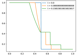
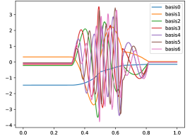
Figure 1: The density $\rho$, solution of the Sod shock tube problem at different timesteps, and the corresponding POD modes (right).

Let $\mathcal{R}$ be the reference domain, similarly to what is used in the Arbitrary Lagrangian Eulerian (ALE) formalism [38], and let $\Omega$ be the physical domain. For every $\bm{\mu}\in\mathcal{P}\subset\mathbb{R}^{s+1}$, we introduce a grid of $M=\prod_{i=1}^{d}M_{i}$ control points that are collected in the vector $\bm{w}(\bm{\mu})\in\Omega^{M}$ that we use for the calibration. These control points should lead the transformation to align the different features at different $\bm{\mu}$. Let $\bm{\alpha}=(\alpha_{1},\dots,\alpha_{d})\in\mathbb{N}^{d}$ be a multi-index with $\alpha_{i}=1,\dots,M_{i}$. Each control point $\bm{w}(\bm{\mu})_{\bm{\alpha}}$ can either belong to the physical domain, i.e., $\bm{w}(\bm{\mu})_{\bm{\alpha}}\in\ring{\Omega}$, or to the boundary of the domain, namely $\bm{w}(\bm{\mu})_{\bm{\alpha}}\in\partial\Omega$. If $\bm{w}(\bm{\mu})_{\bm{\alpha}}\in\partial\Omega$, then this point is constrained for all $\bm{\mu}$ to the boundary hyperplanes where it belongs. We then introduce $\bm{\theta}(\bm{w}(\bm{\mu}))\in\mathbb{R}^{Q}$ that is the vector of the free coordinates of the control points, with $Q\leq d\times M$. We remark that there is a bijection between $\bm{w}$ and $\bm{\theta}$, by definition.
In order to align different features of our set of snapshots, we look for a geometrical transformation map $T\colon\Omega^{M}\times\mathcal{R}\mapsto\Omega$, such that the following properties hold true:

• $T[\cdot]\in\mathcal{C}^{1}(\Omega^{M},\mathcal{C}^{1}(\mathcal{R},\Omega))$;

• $\forall\bm{\mu}\in\mathcal{P}$ and $\forall\bm{w}(\bm{\mu})\in{\Omega^{M}}$, $\exists T^{-1}[\bm{w}(\bm{\mu})]\colon\Omega\mapsto\mathcal{R}$ such that

  $$T^{-1}[\bm{w}(\bm{\mu})](T[\bm{w}(\bm{\mu})]({\hat{\bm{x}}}))={\hat{\bm{x}}}\quad\forall{\hat{\bm{x}}}\in\mathcal{R},$$

  $$T[\bm{w}(\bm{\mu})](T^{-1}[\bm{w}(\bm{\mu})](\bm{x}))=\bm{x},\text{ for all }\bm{x}\in\Omega;$$

• $T^{-1}[\cdot]\in\mathcal{C}^{1}(\Omega^{M},\mathcal{C}^{1}(\Omega;\mathcal{R}))$.

The properties are imposed to setup an ALE formulation [38, 36]. Some possibilities for the geometrical transformation $T$ have been presented in the literature over the past years: among the others we mention here translation maps, dilatation maps, polynomials and Gordon-Hall maps, see [38, 8, 36]. We will use some transformations based on Piecewise Cubic Hermite Interpolation Polynomials (PCHIPs) carefully described in Section 3. In order to use the transformation map $T$, one needs to find the calibration map $\bm{w}\colon\mathcal{P}\mapsto\Omega^{M}$, such that:

• $\bm{w}(\cdot)\in\mathcal{C}^{1}(\mathcal{P};\Omega^{M})$;

• ${\hat{\rho}}(\bm{\mu})({\hat{\bm{x}}}):=\rho(\bm{\mu})(T[\bm{w}(\bm{\mu})]({\hat{\bm{x}}})){\approx}\overline{\rho}({\hat{\bm{x}}})$, for all ${\hat{\bm{x}}}\in\mathcal{R}$, $t\in[0,t_{f}]$ and for all $\bm{\mu}\in\mathcal{P}$, where $\overline{\rho}(\cdot)$ is a reference solution of choice.

Figure 2: Example of a control point grids in 2D with $M_{1}=3$ and $M_{2}=4$ on the reference domain (left) and on the physical domain (right). Note that the coordinates of the reference control points are the tensor product of unidirectional control points

We are now ready to present a general calibration technique: the ultimate goal is to transform the solution manifold $\mathcal{M}_{\rho}$ so that the POD, applied to the transformed manifold, is more efficient. In order to achieve this goal, we need to perform the following steps. First of all we introduce the reference density $\overline{\rho}$, namely a solution of problem (2) for some $\overline{\bm{\mu}}\in\mathcal{P}$. Once $\overline{\rho}$ has been chosen, we select $M$ control points $\overline{\bm{w}}\in\mathcal{R}^{M}$. We consider the $\overline{\bm{w}}$ to be tensor product of points in the interval $[a^{i},b^{i}]$ for every dimension $i=1,\dots,d$, for example in 2D: $\overline{\bm{w}}_{\bm{\alpha}=(\alpha_{1},\alpha_{2})}=(\overline{\bm{w}}^{1}_{\alpha_{1},\alpha_{2}},\overline{\bm{w}}^{2}_{\alpha_{1},\alpha_{2}})$, see Fig. 2. Now, for any $\bm{\mu}\in\mathcal{P}$ and $\bm{w}(\bm{\mu})\in\Omega^{M}$, we can define a geometrical transformation map $T[\bm{w}(\bm{\mu})]\colon\mathcal{R}\mapsto\Omega$ such that

$$\begin{split}T[\bm{w}(\bm{\mu})](\overline{\bm{w}}_{\bm{\alpha}})=\bm{w}_{\bm{\alpha}}(\bm{\mu})\quad\forall\,\bm{\alpha}.\end{split}$$

Once $T[\bm{w}(\bm{\mu})]$ has been defined, we can introduce the calibrated snapshot

$${\hat{\rho}}(\bm{\mu})(\cdot):=\rho(\bm{\mu})(T[\bm{w}(\bm{\mu})](\cdot)).$$

We want to stress that, numerically, we rely on two meshes, one on the physical and one on the reference domain. In our simulations, these two domains will coincide; this does not mean that each transformation map leads to a one-to-one correspondence between the degrees of freedom on the two domains. Hence, we will perform an interpolation of $\rho$ to evaluate $\hat{\rho}$ at its degree of freedom. In the numerical simulations, this procedure will bring an error of the first order of accuracy (as we will use FV approximations).

The map $T[\bm{w}(\bm{\mu})]$ is identified by the control points $\bm{w}(\bm{\mu})$, which are sought in order to minimize the following residual function:

(3) $$\begin{split}R(\rho(\bm{\mu}),\bm{\theta}(\bm{w}(\bm{\mu})),\overline{\rho})=&\lvert\lvert{\hat{\rho}}(\bm{\mu})-\overline{\rho}\rvert\rvert^{2}_{L^{2}(\mathcal{R})}+\frac{\delta}{2}\left\lVert\partial_{\bm{\mu}}\bm{w}(\bm{\mu})\right\rVert^{2}_{\ell^{2}(\mathcal{P})}+\\ &\frac{\alpha}{2}\max_{\bm{x}\in\Omega}\left(\max\left\{\left\lVert\nabla T[\bm{w}(\bm{\mu})](\hat{\bm{x}})\right\rVert,\left\lVert\nabla T^{-1}[\bm{w}(\bm{\mu})](\bm{x})\right\rVert\right\}\right),\end{split}$$

where $\alpha$ and $\delta$ are two penalty parameters user defined, and $\partial_{\bm{\mu}}\bm{w}(\bm{\mu})$ will be defined more in detail in the algorithmic section. We are now ready to present the calibration technique in two different cases: the self-similar setting, and the quasi self-similar one.

2.1 Calibration in the self–similar setting

To keep the presentation as general as possible, we consider here the parametric case, hence $\bm{\mu}=(\mu,t)$ and $\mathcal{P}=\mathcal{P}_{\text{phys}}\times[0,t_{f}]$. We select a training set of physical parameters $\{\mu_{1},\dots,\mu_{N_{\text{train}}}\}=\mathcal{P}_{\text{phys}}^{\text{train}}\subset\mathcal{P}_{\text{phys}}$ and a training set of times $\{t_{1},\dots,t_{N_{\mu}}\}$ for each $\mu\in\mathcal{P}_{\text{phys}}^{\text{train}}$. We then denote $\mathcal{P}^{\text{train}}:=\{\bm{\mu}=(\mu,t):\mu\in\mathcal{P}^{\text{train}}_{\text{phys}}\text{ and }t\in[t_{1},\dots,t_{N_{\mu}}]\}\subset\mathcal{P}$. For each $\bm{\mu}\in\mathcal{P}^{\text{train}}$, we compute the full order model solution $\rho(\bm{\mu})$. We then choose as reference solution $\overline{\rho}=\rho(\bar{\bm{\mu}})$: in our numerical tests we will choose $\bar{\bm{\mu}}~{}=(\mu_{N_{\text{train}}},t_{f})$. In addition to this, we also fix the $M$ reference control points $\overline{\bm{w}}\in\mathcal{R}^{M}$ as specified above.

For all $\bm{\mu}$ in the training set, we solve the following constrained minimization problem:

(4) $$\bm{\theta}^{\text{opt}}(\bm{\mu}):=\min_{\bm{\theta}\in\mathbb{R}^{Q}}R(\rho(\bm{\mu}),\bm{\theta};\overline{\rho}),$$

subject to the following constraints:

• all the control points are within our physical domain: $\bm{w}_{\bm{\alpha}}(\bm{\mu})\in\Omega$ for all $\bm{\alpha}$ and for all training parameters $\bm{\mu}\in\mathcal{P}^{\text{train}}$;

• $\det J[\bm{w}(\bm{\mu})]>0$, where $J[\bm{w}(\bm{\mu})]$ is the Jacobian of the map $T[\bm{w}(\bm{\mu})]$. This constraint must be checked on a quite fine grid of the physical domain $\Omega$, we have used the mesh grid;

• for $i=1,\dots,d$: if $\alpha_{j}=\beta_{j}$ for all $j\neq i$ and $\alpha_{i}<\beta_{i}$, then $\bm{w}_{\bm{\alpha}}^{i}<\bm{w}_{\bm{\beta}}^{i}$ (see Fig. 2), i.e., we never switch the order of the control points on each grid line.

We approximate $\partial_{\bm{\mu}}$ in (3) with the discrete derivative $D_{\bm{\mu}}\bm{w}(\bm{\mu})$ defined as:

$$D_{\bm{\mu}}\bm{w}^{i}_{\bm{\alpha}}(\bm{\mu})=\begin{cases}0&\text{ if }\bm{w}^{i}_{\bm{\alpha}}(\bm{\mu})\text{ is not a free coordinate of }\bm{w}(\bm{\mu});\\ \frac{\bm{\theta}_{q}(\bm{\mu})-\bm{\theta}^{\text{opt}}_{q}(\bm{\mu}_{\text{neigh}}(\bm{\mu}))}{\bm{\mu}-\bm{\mu}_{\text{neigh}}(\bm{\mu})}&\text{with }q\text{ s.t. }\bm{w}^{i}_{\bm{\alpha}}(\bm{\mu})=\bm{\theta}_{q}(\bm{\mu}).\end{cases}$$

In the previous equation, the neighboring parameter $\bm{\mu}_{\text{neigh}}$ is defined as follows:

$$\bm{\mu}_{\text{neigh}}(\bm{\mu},\mathcal{S})=\arg\min_{\bm{\nu}\in\mathcal{S}}\lvert\lvert\bm{\mu}-\bm{\nu}\rvert\rvert_{\ell^{2}(\mathbb{R}^{p+1})},$$

where $\mathcal{S}\subset\mathcal{P}^{\text{train}}$ will contain the parameters for which we have already computed the optimal $\bm{\theta}$. If the minimum is not unique, we take one of the minimizers. The definition of the discrete spatial gradient $\nabla T$ in (3) will be specified in Section 3 for the specific transformation map we use.

Problem (4) is solved with the Sequential Least SQuares Programming (SLSQP) method that is available within the scipy.optimize.minimize library. We solve Problem (4) for the physical parameter $\mu\in\mathcal{P}^{\text{train}}_{\text{phys}}$ for which the solution has more developed structures (the last in our tests): we start from the final timestep $t_{N_{\mu}}$ and we proceed backwards in time. We then move onto solving Problem (4) for the neighboring parameters. In both physical and temporal parameters, the ratio is the following: we proceed form the solutions where the structures that we want calibrate are more developed and we proceed with nearest parameters until we solve the problem for all the training set $\mathcal{P}^{\text{train}}_{\text{phys}}$. The initial guess $\bm{\theta}^{(0)}(\bm{\mu}_{(\ell,j)})$ for $\bm{\mu}_{(\ell,j)}=(\mu_{\ell},t_{j})\in\mathcal{P}^{\text{train}}$ is the optimal output of the minimization for the closest parameter already performed, in our tests it will be defined as:

(5) $$\bm{\theta}^{(0)}(\bm{\mu}_{(\ell,j)})=\begin{cases}\bm{\theta}^{\text{opt}}(\bm{\mu}_{(\ell,j+1)})\text{ if }j=1,\dots,N_{\mu_{\ell}}-1,\\ \bm{\theta}^{\text{opt}}(\bm{\mu}_{(\ell+1,j)})\text{ if }j=N_{\mu_{\ell}}.\end{cases}$$

Algorithm 1 shows the details of the procedure.

Algorithm 1 Calibration for self–similar solution manifold

  Input: the reference solution $\overline{\rho}$, the control points $\overline{\bm{w}}\in\mathcal{R}^{M}$ and the training solution manifold on the physical domain $\{\rho(\mu_{\ell},t_{j})\text{ for }\ell=1,\dots,N_{\text{train}},j=1,\dots,N_{\mu_{\ell}}\}$.

  for $\ell=N_{\text{train}},\dots,1$ do

     for $j=N_{\mu_{\ell}},\dots,1$ do

        Set the initial guess $\bm{\theta}^{(0)}(\bm{\mu}_{(\ell,j)})$ as in (5).

        Solve Problem (4).

     end for

  end for

  Output: the optimal control points $\bm{w}^{\text{opt}}(\bm{\mu}_{(\ell,j)})$.

2.2 Calibration in the quasi–self–similar setting

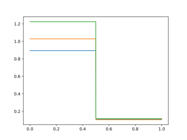
Figure 3: The density $\rho(t=0)$ for three different values of the parameter $\mu=[0.8943,0.1075,1.0906,0.0572]$ (blue), $\mu=[1.0286,0.1031,0.7358,0.0706]$ (orange), and $\mu=[1.2253,0.1157,1.1172,0.1094]$ (green)

To motivate the need of a different algorithm for quasi–self–similar solutions, we focus now on the parametric version of the 1D Sod shock tube problem (2). In this example, the physical parameter $\mu=(\mu^{0},\dots,\mu^{3})\in\mathcal{P}_{\text{phys}}\subset\mathbb{R}^{4}$ represents the IC for the Euler problem:

$$\begin{bmatrix}\rho&u&p\end{bmatrix}^{T}(t=0;\mu)=\begin{cases}\begin{bmatrix}\mu^{0}&0&\mu^{1}\end{bmatrix}^{T}&\text{ if }x<0.5,\\ \begin{bmatrix}\mu^{2}&0&\mu^{3}\end{bmatrix}^{T}&\text{ if }x>0.5.\\ \end{cases}$$

In Fig. 3, we show some analytical solutions for the parametric 1D Sod shock tube, for different values of $\mu$. Looking at Fig. 3 it is clear there is no reasonable choice for the reference solution $\overline{\rho}$ that would lead to reasonable minimization problems, similar to the one presented in Algorithm 1. Indeed, we would minimize the $L^{2}$ error between two solutions ($\overline{\rho}$ and ${\hat{\rho}}(\bm{\mu})$) that may have very different heights at the boundaries just changing the geometrical transformation. When different boundaries behaviors are present, the calibration procedure needs to be reformulated in a different way.

Instead of fixing $\overline{\rho}$, we minimize the projection error onto a suitable reduced space $V_{\textrm{POD}}$ in the following way:

(6) $$\begin{split}\min_{\bm{\theta}({\bm{\mu}})\in\mathbb{R}^{Q}}&\lVert{\hat{\rho}}({\bm{\mu}})-\Pi_{V_{\textrm{POD}}}{\hat{\rho}}({\bm{\mu}})\rVert_{L^{2}(\mathcal{R})}+\frac{\delta}{2}\lVert\partial_{\bm{\mu}}\bm{w}(\bm{\mu})\rVert^{2}_{\ell^{2}(\mathcal{P})}+\\ &\frac{\alpha}{2}\max_{\bm{x}\in\Omega}\left(\max\left\{\left\lVert\nabla T[\bm{w}(\bm{\mu})](\hat{\bm{x}})\right\rVert,\left\lVert\nabla T^{-1}[\bm{w}(\bm{\mu})](\bm{x})\right\rVert\right\}\right),\end{split}$$

with $\bm{\theta}$ constrained as in the previous section and $\Pi_{V_{\textrm{POD}}}$ the orthogonal projection onto a linear space $V_{\textrm{POD}}$ obtained through a preliminary procedure that we will describe later on.

This minimization allows to overcome the issue of quasi–self–similar solutions thanks to the projection onto a reduced space. To do so, we need to find a priori a suitable reduced space $V_{\textrm{POD}}$ that comprises the minimal information of the solution manifold: for this reason, from the training set $\mathcal{P}^{\text{train}}$ we select few parameters $\tilde{\bm{\mu}}_{1},\dots,\tilde{\bm{\mu}}_{N_{\text{few}}}$, with $N_{\text{few}}\ll\sum_{i=1}^{N_{\text{train}}}N_{\mu_{i}}$.

We then introduce the matrix of the free coordinates $\overrightarrow{\theta}\in\mathbb{R}^{N_{\text{few}}\times Q}$, where:

$$\overrightarrow{\theta}[i,:]=\bm{\theta}(\tilde{\bm{\mu}}_{i}),\quad i=1,\dots,N_{\text{few}}.$$

The free coordinates can be selected through another optimization process carried out in the same spirit of (6) on the whole matrix $\overrightarrow{\theta}$, minimizing the projection error over all the parameters $\tilde{\bm{\mu}}_{1},\dots,\tilde{\bm{\mu}}_{N_{\text{few}}}$, while updating the space $V_{\textrm{POD}}$ obtained by compressing the solutions on the reference domain for these parameters. Therefore, we solve the following constrained minimization problem:

(7) $$\min_{\overrightarrow{\theta}\in\mathbb{R}^{N_{\text{few}}\times Q}}\sum_{i=1}^{N_{\text{few}}}\lVert{\hat{\rho}}(\tilde{\bm{\mu}}_{i})-\Pi_{V_{\textrm{POD}}}{\hat{\rho}}(\tilde{\bm{\mu}}_{i})\rVert_{L^{2}(\mathcal{R})}\text{ with }V_{\textrm{POD}}:=\textrm{POD}(\{{\hat{\rho}}(\tilde{\bm{\mu}}_{i})\}_{i=1}^{N_{\text{few}}},N^{\textrm{POD}}_{\text{few}}).$$

This optimization process is of larger dimension with respect to the previous ones and it requires, for each residual evaluation, the computation of a POD over the $N_{\text{few}}$ calibrated snapshots ${\hat{\rho}}(\tilde{\bm{\mu}}_{i})$, with a user defined number of modes $N_{\text{few}}^{\textrm{POD}}$, which must be chosen trying to keep into account all the possible independent components of the problem between different travelling features. In the Sod test case, we have chosen $N_{\text{few}}^{\textrm{POD}}=3$ to keep into account the different values that there might be between the rarefaction and the contact discontinuity and between the contact and the shock. $N_{\text{few}}^{\textrm{POD}}$ should be kept as low as possible not to overload the minimization process: in the Sod test case, we did few tests with increasing $N_{\text{few}}^{\textrm{POD}}$ and $3$ was the first value where the minimization process was giving successful results. Again, we solve problem (7) with SLSQP using the same constraints defined in the previous section. This extra optimization step can be skipped when other techniques to detect interesting features can be used [11]. One possibility is the use of classical shock detection procedures to find the steepest points of the solutions and calibrating them [23]. We summarize the steps of the whole procedure in Algorithm (2).

Algorithm 2 Calibration for quasi–self–similar solution manifold

  Input: the training solution manifold on the physical domain $\{\rho(\mu_{\ell},t_{j})\text{ for }\ell=1,\dots,N_{\text{train}},j=1,\dots,N_{\mu_{\ell}}\}$ and the number of modes $N^{\textrm{POD}}_{\text{few}}$.

  Select few parameters $\tilde{\bm{\mu}}_{1},\dots,\tilde{\bm{\mu}}_{N_{\text{few}}}$.

  Find optimal $\overrightarrow{\theta}\in\mathbb{R}^{N_{\text{few}}\times Q}$ by (7) for the few parameters $\tilde{\bm{\mu}}_{1},\dots,\tilde{\bm{\mu}}_{N_{\text{few}}}$.

  for $\ell=N_{\text{train}},\dots,1$  do

     for $j=N_{\mu_{\ell}},\dots,1$ do

        Set the initial guess $\bm{\theta}^{(0)}(\bm{\mu}_{(\ell,j)})$ as in (5).

        Solve Problem (4).

     end for

  end for

  Output: the optimal control points $\bm{w}^{\text{opt}}(\bm{\mu}_{(\ell,j)})$.

3 The geometrical transformation map

We now present the geometrical transformation map $T[\bm{w}^{\text{opt}}(\bm{\mu})]\colon\mathcal{R}\mapsto\Omega$ used to define the calibrated snapshots. We start with the simpler case, namely the 1D setting, and later we consider the 2D case.

3.1 The 1D setting

Let $\bm{w}^{\text{opt}}(\bm{\mu})$ be the control points whose free coordinates are the solution to Problem (4): to interpolate the values $\{(\overline{\bm{w}}_{\bm{\alpha}}(\bm{\mu}),\bm{w}^{\text{opt}}_{\bm{\alpha}}(\bm{\mu}))\}_{\bm{\alpha}}$, we use monotone cubic $C^{1}$ splines. These are the so-called PCHIPs (Piecewise Cubic Hermite Interpolating Polynomials) interpolators, available in the scipy Python library under the interpolate classes and the built-in function is called PchipInterpolator. By employing monotone cubic splines, we obtain a transformation function that preserves the monotonicity of the calibration map $\bm{w}(\cdot)$, guaranteeing its bijectivity and $C^{1}$ smoothness if the calibration points are in the “right order”, as prescribed in Section 2.

Figure 4: Example of PCHIP calibration: solution on physical domain (left) with calibration control points (left), solution on reference domain with reference control points (center) and PCHIP transformation with all control points (right)

In Fig. 4, we can see an example of a PCHIP transformation applied to one of the snapshot calibrated on the detected features. On the right of the figure, the transformation is depicted and we can observe that it interpolates the points, it is $\mathcal{C}^{1}$ and it is very close to the identity on the boundaries, because we introduce two extra interpolation points outside the boundaries of the domain. This helps to keep the regularity of the transformation in the ALE formulation [36].

In this work, we do not focus on the ALE formulation on $\mathcal{R}$, nevertheless the PCHIPs allow to easily compute all the necessary ingredients. Indeed, they are polynomials and their derivatives and the inverse of their derivative is easy to compute. Moreover, the inverse of the transformation exists and it is unique in each point, hence, with a simple Newton method, we can easily recast the inverse function.

3.2 The 2D setting

In the 2D setting we use tensor product of one dimensional PCHIPs, in order to exploit their properties for Cartesian geometries. We refer again to Fig. 2 to better understand the transformation map. We need to compute $T[\bm{w}^{\text{opt}}(\bm{\mu})]\colon\mathcal{R}\mapsto\Omega$, such that

$$T[\bm{w}^{\text{opt}}(\bm{\mu})](\overline{\bm{w}}^{1}_{\alpha_{1},\alpha_{2}},\overline{\bm{w}}^{2}_{\alpha_{1},\alpha_{2}})=(\bm{w}^{1,\text{opt}}_{\alpha_{1},\alpha_{2}}(\bm{\mu}),\bm{w}^{2,\text{opt}}_{\alpha_{1},\alpha_{2}}(\bm{\mu}))\quad\text{ for }\alpha_{i}=1,\dots,M_{i},\,i=1,2.$$

Let ${\hat{\bm{x}}}\in\mathcal{R}$ be a point with coordinates ${\hat{\bm{x}}}=(\hat{x},\hat{y})$. We define the map:

$$T[\bm{w}^{\text{opt}}(\bm{\mu})](\hat{x},\hat{y}) :=(T^{x}[\bm{w}^{\text{opt}}(\bm{\mu})](\hat{x},\hat{y}),T^{y}[\bm{w}^{\text{opt}}(\bm{\mu})](\hat{x},\hat{y})),\text{ with }$$

$$T^{x}[\bm{w}^{\text{opt}}(\bm{\mu})](\hat{x},\hat{y}) :=\sum_{\ell=1}^{M_{2}}{\gamma}^{y}_{\ell}(\hat{y})P^{x}_{\ell}(\hat{x}),\qquad T^{y}[\bm{w}^{\text{opt}}(\bm{\mu})](\hat{x},\hat{y}):=\sum_{k=1}^{M_{1}}{\gamma}^{x}_{k}(\hat{x})P^{y}_{k}(\hat{y}).$$

In the previous equations, we made use of the following quantities:

1. $P^{x}_{\ell}$ is a PCHIP interpolating the points $\{\overline{\bm{w}}^{1}_{\alpha_{1},\ell},\bm{w}^{1,\text{opt}}_{\alpha_{1},\ell}(\bm{\mu})\}_{\alpha_{1}=1}^{M_{1}}$, where the control points $\overline{\bm{w}}^{1}_{\alpha_{1},\ell}$ for $\alpha_{1}=1,\dots,M_{1}$ are on horizontal lines $\hat{y}=\bar{y}_{\ell}$ in the reference domain, see Fig. 2, namely for all $\alpha_{1}=1,\dots,M_{1}$ we have $P^{x}_{\ell}(\overline{\bm{w}}^{1}_{\alpha_{1},\ell})=\bm{w}^{1,\text{opt}}_{\alpha_{1},\ell}(\bm{\mu});$

2. $P^{y}_{k}$ is a PCHIP interpolating the points $\{\overline{\bm{w}}^{2}_{k,\alpha_{2}},\bm{w}^{2,\text{opt}}_{k,\alpha_{2}}(\bm{\mu})\}_{\alpha_{2}=1}^{M_{2}}$, where the control points $\overline{\bm{w}}^{2}_{k,\alpha_{2}}$ for $\alpha_{1}=1,\dots,M_{1}$ are on vertical lines $\hat{x}=\bar{x}_{k}$ in the reference domain, see Fig. 2, namely for all $\alpha_{2}=1,\dots,M_{2}$ we have $P^{y}_{k}(\overline{\bm{w}}^{2}_{k,\alpha_{2}}(\bm{\mu}))=\bm{w}^{2,\text{opt}}_{k,\alpha_{2}}(\bm{\mu});$

3. ${\gamma}^{y}_{\ell}(\cdot)$ is a PCHIP interpolating the points $\{\overline{\bm{w}}^{2}_{\alpha_{1},\alpha_{2}},\delta_{\alpha_{2},\ell}\}_{\alpha_{2}=1}^{M_{2}}$, being $\delta_{\alpha_{2},\ell}$ the Kronecker delta. By doing so, we obtain that $T^{x}[\bm{w}^{\text{opt}}(\bm{\mu})]$ is a convex combination of the $\{P^{x}_{\ell}(\cdot)\}_{\ell=1}^{M_{2}}$ such that $T^{x}[\bm{w}^{\text{opt}}(\bm{\mu})](\hat{x},\hat{y}=\overline{\bm{w}}^{2}_{\alpha_{1},\alpha_{2}})=P^{x}_{\alpha_{2}}(\hat{x})$;

4. ${\gamma}^{x}_{k}(\cdot)$ is a PCHIP interpolating the points $\{\overline{\bm{w}}^{1}_{\alpha_{1},\alpha_{2}},\delta_{\alpha_{1},k}\}_{\alpha_{1}=1}^{M_{1}}$, as before, leading to the property $T^{y}[\bm{w}^{\text{opt}}(\bm{\mu})](\hat{x}=\overline{\bm{w}}^{1}_{\alpha_{1},\alpha_{2}},\hat{y})=P^{y}_{\alpha_{1}}(\hat{y})$.

Notice that, ultimately, it holds that

$$T[\bm{w}^{\text{opt}}(\bm{\mu})](\overline{\bm{w}}^{1}_{\alpha_{1},\alpha_{2}},\overline{\bm{w}}^{2}_{\alpha_{1},\alpha_{2}})=(P_{\alpha_{2}}^{x}(\overline{\bm{w}}^{1}_{\alpha_{1},\alpha_{2}}),P_{\alpha_{1}}^{y}(\overline{\bm{w}}^{2}_{\alpha_{1},\alpha_{2}}))=\bm{w}^{\text{opt}}_{\alpha_{1},\alpha_{2}}(\bm{\mu}).$$

Also in the 2D case, the Jacobian of the transformation, which is needed in the ALE formulation, is easily accessible, since all the terms are polynomials. Similarly to the 1D case, we can compute the Jacobian of the inverse of the transformation, using the inverse of the Jacobian of the transformation, provided that we can invert the map $T$.

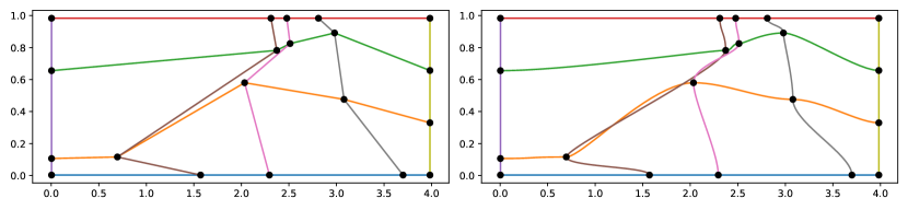
Figure 5: Calibration points ($M_{1}=5,M_{2}=4$) on the physical domain $\Omega=[0,4]\times[0,1]$ so that they respect the monotonicity in each line (left), but whose transformed horizontal and vertical lines cross multiple times (right)

Remark 3.1 (Invertibilty of $T$).

The computation of the inverse of $T$ is fundamental in many aspect of the algorithm: to display the function on the physical domain, to compute quantities and errors on the physical domain and to compute the inverse of the Jacobian for the ALE formulation.

Unfortunately, the so defined map $T$ cannot be proven to be invertible, as it might happen that some of the vertical and horizontal lines cross each other multiple times in the physical domain, see Fig. 5. To avoid this, we impose, in the optimization procedure for the calibration, to have positive determinant of the Jacobian of the transformation on the meshpoints of the reference domain, see the constraints in Section 2.1. This typically guarantees invertibility. We recall that, being PCHIPs polynomials, the computation of the Jacobian can be performed explicitly in each point. To compute the inverse of the transformation, we perform the following steps. We first apply the transformation map $T$ to the elements of the Cartesian meshgrid of $\mathcal{R}$: these will be mapped to quadrilateral elements in $\Omega$. Now, given a point $\bm{x}\in\Omega$, we can easily find to which of these quadrilaterals it belongs and with a Projective transformation (see the python module transform of the package skimage) we pull it back onto $\mathcal{R}$. Then, we use the found point as initial guess to find the solution of $T[\bm{w}^{\text{opt}}(\bm{\mu})](\hat{\bm{x}})=\bm{x}$ through a Newton type nonlinear solver (scipy.root).

4 Model Order Reduction with calibration

We are now ready to perform the model order reduction step. In what follows the procedure is similar for the non parametric and the parametric setting: we will therefore present it for the latter case, for the sake of generality.

4.1 Learning the calibration map

Once the calibration procedure presented in Section 2 has been carried out, the map $\bm{w}\colon\mathcal{P}\mapsto\Theta$ is known only through the sample values $\bm{w}^{\text{opt}}(\bm{\mu})$, for $\bm{\mu}\in\mathcal{P}^{\text{train}}$. To learn the calibration map $\bm{w}(\cdot)$ for any parameter $\bm{\mu}$, we employ an Artificial Neural Network (ANN) composed by several layers: an input layer $\bm{\mu}\in\mathcal{Y}^{(0)}=\mathcal{P}$ where we pass the parameters of the problem of interest, L hidden layers $\mathcal{Y}^{(j)}$, $j=1,\dots,L$, and an output layer $\mathcal{Y}^{(L+1)}$, see Fig. 6. As output layer, we would like to obtain $\bm{\theta}\in\mathbb{R}^{Q}$, from which we can extract the calibration points $\bm{w}$. Keeping in mind the monotonicity constraints applied to the control points in the constrained minimization problems (4) and (6), we try to enforce this constraint in the ANN. It is not easy to strongly enforce such constraints, but we can force the output to be positive, using as final activation function a Softplus. Hence, we take as output layer of our ANN not directly $\bm{\theta}$, but the vector $\bm{v}\in\mathbb{R}^{Q}$ of the differences of the free coordinates with the previous ones (in 2D it is referred to the same line). Doing so, the positivity of $\bm{v}$ is equivalent to the monotonicity in each line of points. In one dimension, it is defined as $v_{i}=w_{i}-w_{i-1}$ for $i=2,\dots,M_{1}-1$, while in two dimensions this operation is done in each horizontal or vertical line.

Figure 6: Example of the architecture of an ANN

Each layer $\mathcal{Y}^{(j)}$, $j=1,\dots,L$ is connected to the next and to the previous ones through affine maps $\delta^{(j)}\colon\mathcal{Y}^{(j)}\mapsto\mathcal{Y}^{(j+1)}$ and at every node a nonlinear activation function $\zeta^{(j)}\colon\mathbb{R}\mapsto\mathbb{R}$ is applied component–wise. We used the hyperbolic tangent in all the ANN except in the output layer where the Softplus function is used for the positivity of the outputs. On a training set, the learning process changes the weights $\delta^{(k)}$ minimizing the error between the output and the optimal calibration points.

To build and train the ANN, we used a Python based library EZyRB [10] that uses Adam method [20] to perform the minimization. More details on the architecture of the ANN for the different test cases will be provided in the numerical section.

4.2 POD-NN

In Section 2.1 and 2.2, we presented the calibration algorithm in the self-similar and in the quasi self-similar setting. Thanks to the calibration of the snapshots, we obtain the calibrated manifold $\hat{\mathcal{M}}_{\rho}=\{{\hat{\rho}}(\bm{\mu})(\cdot),\text{ }\bm{\mu}\in\mathcal{P}_{\text{train}}\}$, where ${\hat{\rho}}(\bm{\mu})(\cdot)$ is the calibrated snapshot defined in Section 2. We now proceed with the compression of $\hat{\mathcal{M}}_{\rho}$ by means of the Proper Orthogonal Decomposition (POD): we refer to [15] for more details. The dimension of the reduced basis can be chosen either setting a maximum number of basis $N^{\text{max}}_{\text{POD}}$ or choosing the most relevant modes such that the discarded energy is smaller than a certain tolerance $\tau_{\text{POD}}$. Once the POD has been carried out, we obtain a linear space $V^{\rho}_{N}$ spanned by the $N$ orthonormal reduced basis functions $\{\hat{\Phi}_{i}\}_{i=1}^{N}$ on the reference domain $\mathcal{R}$. $V^{\rho}_{N}$ should now represent with a good accuracy any element of the calibrated solution manifold $\hat{\mathcal{M}}_{\rho}$.

4.3 Online solution by means of ANN

In this work, we mainly focus on the calibration procedure and the offline phase. Hence, we will use a non–intrusive approach for the reconstruction of the online solutions. Let $\bm{\mu}\in\mathcal{P}$ be a parameter of choice: the goal is to construct a linear approximation $\rho_{N}(\bm{\mu})$ of the snapshot $\rho(\bm{\mu})$. It should be clear by now that, since we are dealing with advection dominated problems, this is not a simple task within the standard MOR setting. However, in Sections 2 and 3, we presented a calibration technique that allows us to obtain a linear space $V^{\rho}_{N}$ that approximates with good accuracy the calibrated manifold $\hat{\mathcal{M}}_{\rho}$: we are therefore able to construct a linear approximation of the calibrated solution of interest ${\hat{\rho}}(\bm{\mu})$ in the reference domain $\mathcal{R}$. This means that we can approximate ${\hat{\rho}}(\bm{\mu})$ with

(8) $${\hat{\rho}}(\bm{\mu})\approx{\hat{\rho}}_{N}(\bm{\mu}):=\sum_{i=1}^{N}\underline{{\hat{\rho}}}_{N}^{i}(\bm{\mu})\hat{\Phi}_{i},$$

(9) where $$\underline{{\hat{\rho}}}_{N}^{i}(\bm{\mu})=({\hat{\rho}}(\bm{\mu}),\hat{\Phi}_{i})_{L^{2}(\mathcal{R})}\quad\text{ for }i=1,\dots,N,$$

being $(\cdot,\cdot)_{L^{2}(\mathcal{R})}$ the $L^{2}$ scalar product on the reference domain. In order to find the vector $\underline{{\hat{\rho}}}_{N}(\bm{\mu})$ one can adopt two alternative ways: an intrusive approach, by means of a Galerkin projection of the high order algebraic system onto the reduced space, or a non-intrusive approach by means of an ANN. If the standard Galerkin projection setting is adopted, the online system and the reconstruction of the online solution is carried out within an ALE formalism [32, 38, 36]: the original problem of interest, formulated over $\Omega$, has to be re-written into a problem formulated over the reference domain $\mathcal{R}$. In this approach, a hyper-reduction procedure [4, 41] will be necessary to tackle the nonlinearities of the problem and of the transformation map. This approach is currently under investigation, and it will be part of a future extensions.

An alternative to the intrusive approach is represented by the use of ANN, in the spirit of Section 4.1. We consider the map $\Pi_{N}\colon\mathcal{P}\mapsto\mathbb{R}^{N}$

$$\begin{split}\Pi_{N}(\bm{\mu}):=\underline{{\hat{\rho}}}_{N}(\bm{\mu})=[\underline{{\hat{\rho}}}_{N}^{1}(\bm{\mu}),\dots,\underline{{\hat{\rho}}}_{N}^{N}(\bm{\mu})]^{T}.\end{split}$$

We make use of an ANN to learn the $L^{2}$ projection map $\Pi_{N}$: to train the map, we employ the set of input samples $\bm{\mu}$ for $\bm{\mu}\in\mathcal{P}^{\text{train}}$, and the set of output samples $\{\underline{{\hat{\rho}}}_{N}(\bm{\mu})\text{ for }\bm{\mu}\in\mathcal{P}^{\text{train}}\}$. In this algorithm, we do not use the optimal calibrated points obtained with the optimization process, but we use the ones predicted by the ANN of Section 4.1. Doing so, any systematic error in the online calibration should be already taken into account while performing the $L^{2}$ projection and automatically corrected by this approach. Moreover, it is also possible to use different training sets for the calibration optimization procedure and the model order reduction ones. More details on the architecture of the ANN employed will be provided in the numerical section.

5 Numerical results

We now present some numerical results to validate the proposed methodology. We will consider four different time dependent test cases: the Sod shock tube problem in 1D, in the non parametric and in the parametric setting, already introduced in Section 2.1 and 2.2, respectively. To further test the performance of our methodology, we subsequently consider a 2D problem, namely the double Mach reflection (DMR) problem, again in the non parametric and in the parametric setting.

5.1 Non-parametric Sod shock tube problem in 1D

We consider Problem (2) introduced in Section 1.1, where the physical domain is $\Omega=\mathcal{R}=[0,1]$. To obtain the high order solutions, we employ an explicit Finite Volume discretization with WENO reconstruction of order 5, with time discretization given by the optimal SSPRK54, with CFL coefficient 0.8 and Rusanov numerical flux. The number of spatial degrees of freedom is 1500 and this leads to computational costs of around 2 minutes using a Fortran code [27] on a Intel(R) Xeon(R) CPU E3-1245 v5 @ 3.50GHz. In both cases, we use Dirichlet BC as the waves do not exit the domain before the final time. The details of all the relevant quantities are presented in Table 1.

Table 1: Test details for the 1D Sod shock tube problem, non parametric (Nonparam) and parametric (Param) setting

Quantity	Nonparam	Param	Quantity	Nonparam	Param
$\rho_{L}$	$1$	$[0.7,1.3]$	$\rho_{R}$	$0.1$	$[0.1,0.15]$
$u_{L}$	$0$	0	$u_{R}$	0	$0$
$p_{L}$	$1$	$[0.7,1.3]$	$p_{R}$	$0.125$	$[0.05,0.15]$
$t_{f}$	$0.2$s	$0.2$s	$N_{h}$	1500	1500

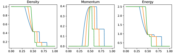
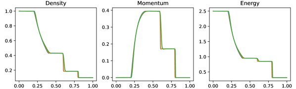
Figure 7: FOM simulation of Sod 1D problem non parameteric at times 0.04 (green), 0.1 (orange) and 0.16 (blue), on the original domain (top) and calibrated on the reference domain (bottom)

Fig. 7 shows some snapshots for the density $\rho$, the moment $m$ and the energy $E$ at three different times of the simulation: it is clear that the structures of all three the components of the solution present discontinuities that travel in the domain at the same locations.

We carry out the calibration technique proposed in Algorithm 1: we choose as reference solution $\overline{\rho}$ the density $\rho(t=0.16)$. We then choose $M=4$ control points $\overline{\bm{w}}_{1}=0.2,\,\overline{\bm{w}}_{2}=0.4,\,\overline{\bm{w}}_{3}=0.6,\,\overline{\bm{w}}_{4}=0.8$ equispaced in the reference domain $\mathcal{R}=[0,1]$. The calibrated solutions (using the ANN to forecast the calibration points) are shown in Fig. 7: the main features of the solutions, namely the shock, the contact discontinuity and the rarefaction wave are well aligned with the reference solution. The details of the quantities required to carry out the calibration step are listed in Table 2. We point out that the calibration step and the training of the ANN have been carried out on the training set $\mathcal{P}^{\text{train}}\subset[0.01,0.16]\subset[0,0.2]$ sampled with 25 equispaced parameters. The reason for excluding the first timesteps from the training is that the minimization is tricky during the first timesteps: indeed we have a transition phase, during which all the features are in the same point, leading to non invertible maps. An alternative way to overcome this difficulty could be to restore to local reduced basis spaces [2], or to use a FOM approach for the first timesteps. The final times are excluded to test the extrapolatory performances of the ROM.

Figure 8: Sod 1D: Eigenvalue decay of the PODs (normalized to have $\lambda_{1}=1$) non parametric (left) and parametric (right)

Table 2: Calibration of the 1D Sod shock tube problem, non parametric and parametric setting

Quantity	Nonparam	Param	Quantity	Nonparam	Param
$\delta$	$10^{-6}$	$10^{-6}$	$\alpha$	$0.$	$0.$
$\overline{\rho}$	$\rho(t=0.16)$	-	$M_{1}$	6	6
max. iter.	$100$	$100$	minim. alg.	SLSPQ	SLSPQ
$N_{\text{train}}$	1	$16$	$N_{\mu}$	25	25
$N_{\text{few}}$	-	$10$	$N^{\text{POD}}_{\text{few}}$	-	$3$

Table 3: Architecture and details of the calibration-NN and the POD-NN in both non parametric and parametric setting

	Non parametric case		Parametric case
Parameter	Calibration-NN	POD-NN	Calibration-NN	POD-NN
$L$	$4$	4	$4$	4
neurons per layer	$16$	$16$	16	16
max. epochs	$20000$	$10000$	$20000$	$10000$
loss fun. tol.	$10^{-6}$	$10^{-5}$	$10^{-6}$	$10^{-5}$
$\tilde{\zeta}$	Tanh/Softplus	Tanh	Tanh/Softplus	Tanh
$\tau_{\text{POD}}$	-	$10^{-4}$	$10^{-4}$	$10^{-4}$
$N^{\text{max}}_{\text{POD}}$	-	$7$	3	7

Eulerian approach
   
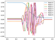
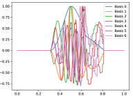
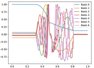
ALE approach
   

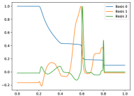
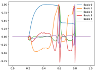
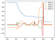
Figure 9: Sod 1D non parametric: The first modes obtained by compressing the original manifolds (Eulerian on the top) and the calibrated manifolds (ALE on the bottom) for $\rho$ (left), $m$ (center) and $E$ (right), with POD with $\tau_{\text{POD}}=10^{-4}$ and $N^{\text{max}}_{\text{POD}}=7$

Eulerian ROM
   
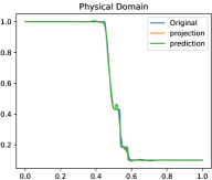
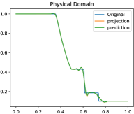
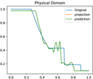
ALE ROM
   

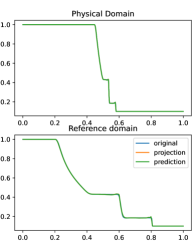
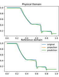
Figure 10: Sod 1D non parametric: Online approximation of the density $\rho$ at times 0.04, 0.12 and 0.2 (left to right). Top row: Eulerian ROM simulations with $N=7$ modes on $\Omega$. Central row: ALE ROM simulations on $\Omega$ with $N=3$ modes. Bottom row: ALE ROM simulations on $\mathcal{R}$ with $N=3$ modes

Fig. 8 (left) shows the eigenvalue decay of the POD for both calibrated (ALE, in blue) and original (Eulerian, in red) approaches. We can see that, differently from the Eulerian approach, for the calibrated approach the first eigenvalue is much more relevant than all the others and the Kolmogorov $n$–width decay is much faster. Fig. 9 shows the behavior of the first modes obtained by compressing with a POD the non-calibrated manifolds, for the three conservative variables $\rho$, $m$ and $E$. We remark that also here we consider the FOM solutions for $t\in\mathcal{P}^{\text{train}}$, thus excluding the initial and the final times from the compression. The modes are highly oscillatory, because they struggle to correctly represent the positions of the three discontinuities in the domain. Fig. 9 also shows the POD modes obtained by running a POD on the calibrated manifolds: after the calibration the oscillations in the modes are much milder and focused on the discontinuity locations. Fig. 10 shows some POD-NN results with $N=7$, without calibration, for the density $\rho$ at different times $t$ (including the extrapolatory regime at $t=0.2$). The comparison is made between the FOM solution $\rho$, its $L^{2}$ projection onto the reduced space generated by the first $N=7$ modes of the non-calibrated manifold (Eulerian modes) and the online reconstruction obtained using a linear combination of said modes, with coefficients that are predicted by an ANN. We can see that the Eulerian approach fails to correctly reproduce the calibrated FOM solutions: in particular, the standard MOR struggles to capture the correct position of the discontinuities, and it shows some oscillations in the online approximation that are most likely due the highly oscillating nature of the Eulerian modes themselves. Fig. 10 also shows some POD-NN simulations obtained after the calibration procedure (computational cost of prediction of both calibration points and ROM coefficients below 0.001s); here we use $N=3$ modes as the POD algorithm stops earlier for the imposed tolerance. We can see that we obtain a very good approximation of the calibrated snapshots in the reference configuration $\mathcal{R}$, i.e., ${\hat{\rho}}$, and in the physical domain $\Omega$, i.e. $\rho$, with the main features correctly reproduced by the online solution. We stress the fact that $t=0.2$ is outside the training interval $\mathcal{P}^{\text{train}}$: in this case, the positions of the shock, the contact and the rarefaction wave have been slightly misplaced by the online model, hence, the approximation is not as great as in the interpolatory regime. All the details on the architecture of the ANN used to learn the calibration map and to predict the online solution are summarized in Table 3.

5.2 Parametric Sod shock tube problem in 1D

Eulerian approach
   
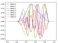
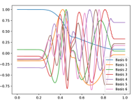
ALE approach

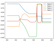
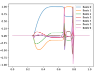
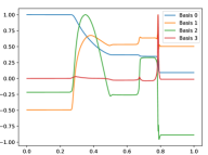
Figure 11: Sod 1D parametric: The first modes obtained by compressing the original manifolds (Eulerian on the top) and the calibrated manifolds (ALE on the bottom) for $\rho$ (left), $m$ (center) and $E$ (right), with POD with $\tau_{\text{POD}}=10^{-4}$ and $N^{\text{max}}_{\text{POD}}=7$

Eulerian ROM
   
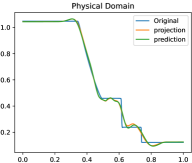
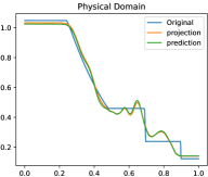
ALE ROM
   

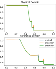
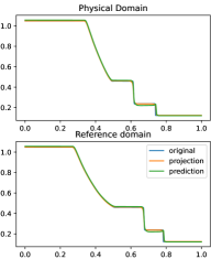
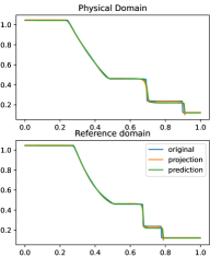
Figure 12: Sod 1D parametric: Online approximation of the density $\overline{\rho}$ at times 0.04, 0.12 and 0.2 (left to right), for $\rho_{L}=1.047937,\,\rho_{R}=0.122810,\,p_{L}=1.203980,\,p_{R}=0.144468$. Top row: Eulerian ROM simulations on $\Omega$ with $N=7$ modes. Central row: ALE ROM simulations on $\Omega$ with $N=4$ modes. Bottom row: ALE ROM simulations on $\mathcal{R}$ with $N=4$ modes

Eulerian ROM
   
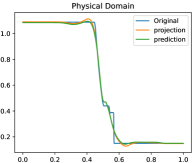
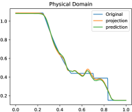
ALE ROM
   

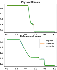
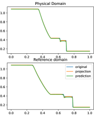
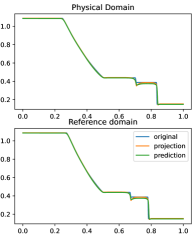
Figure 13: Sod 1D parametric: Online approximation of the density $\overline{\rho}$ at times 0.04, 0.12 and 0.2 (left to right), for $\rho_{L}=1.08827,\,\rho_{R}=0.149654,\,p_{L}=1.193154,\,p_{R}=0.078459$. Top row: Eulerian ROM simulations on $\Omega$ with $N=7$ modes. Central row: ALE ROM simulations on $\Omega$ with $N=4$ modes. Bottom row: ALE ROM simulations on $\mathcal{R}$ with $N=4$ modes

We now consider the parametric version of the Sod problem, already introduced in Section 2.2. We recall that we consider $\mu=(\rho_{L},\rho_{R},p_{L},p_{R})\in\mathcal{P}_{\text{phys}}\subset\mathbb{R}^{4}$. All the details for the numerical simulations are provided in Table 1. Also in this case, the FOM solutions have been obtained employing the same FV discretization. In the parametric setting, we generate the training space $\mathcal{P}_{\text{phys}}^{\text{train}}$ using $N_{\text{train}}=16$ randomly selected parameters $\mu$ from $\mathcal{P}_{\text{phys}}$. Again, we consider the training time interval $[0.01,0.16]$ discretized with around 45 times for each physical parameter.

Fig. 11 shows the first modes for the three components $\rho$, $m$ and $E$, without calibration (Eulerian approach) and with calibration (ALE approach), respectively. Also in the parametric case, we can notice that the Eulerian modes are highly oscillating, similarly to the non-parametric test case: the calibration helps to significantly mitigate this phenomenon. To further validate this, we show in Fig. 8 (right) a comparison between the rate of decay of the eigenvalues obtained with a POD on the non-calibrated (red) and calibrated (blue) manifolds. The calibration results in an improvement in the rate of decay and we clearly observe that, in comparison to the non parametric case, the decay is slower and we need more basis functions to represent our solution manifold. All the details for the numerical implementation of the calibration procedure are summarized in Table 2.

Fig. 12 and Fig. 13 represent the FOM, the $L^{2}$ projection on the reduced space and the POD–NN online approximation for $\rho$, for two parameters in the test set. We plot both the Eulerian ROM and the ALE one, for the latter both in the physical $\Omega$ and in the reference domain $\mathcal{R}$. The online approximations are obtained with $N=4$ modes. As we can see, in both cases the Eulerian ROM is struggling to correctly capture the positions of the discontinuities, and it provides an approximated solution that exhibits some non-negligible oscillations, most likely due to the oscillating nature of the Eulerian modes themselves. The results provided with the calibration are much more accurate, since the MOR is now able to correctly represent the positions of the discontinuities, and it does not present any oscillations in the approximations. There are minor flaws in the extrapolatory regime and in the early times, still keeping the quality of the reduced solution very high.

All the details on the architecture of the ANN used to learn the calibration map and to predict the online solution are summarized in Table 3.

5.3 Non-parametric DMR problem in 2D

We now consider a 2D test case, namely the Double Mach Reflection (DMR) problem [40]. Let $\Omega=[0,4]\times[0,1]$: we consider the Euler equations (2), in the time interval $[0,0.25]$, with the following IC

(10) $$\begin{cases}(\rho_{L},u_{L},v_{L},p_{L})=(8,8.25\cos(\beta),-8.25\sin(\beta),116.5)&\bm{x}\in\Omega_{L}(\beta,t=0)\\ (\rho_{R},u_{R},v_{R},p_{R})=(1.4,0,0,1)&\bm{x}\in\Omega_{R}(\beta,t=0)\end{cases}$$

(11) $$\Omega_{L}(\beta,t)=\left\{\bm{x}\in\Omega:x<\frac{1}{6}+\tan(\beta)y+\frac{10}{\cos(\beta)}t\right\},\qquad\Omega_{R}(\beta,t)=\Omega\setminus\Omega_{L}(\beta,t),$$

with $\beta=\frac{\pi}{6}$. The BCs are assigned through ghost cells as

(12) $$(\rho,u,v,p)=\begin{cases}(\rho_{L},u_{L},v_{L},p_{L}),&\text{if }x=0\text{ or }(y=1\text{ and }\bm{x}\in\Omega_{L}(\beta,t)),\\ (\rho_{R},u_{R},v_{R},p_{R}),&\text{if }y=1\text{ and }\bm{x}\in\Omega_{R}(\beta,t),\\ (\rho_{in},u_{in},-v_{in},p_{in}),&\text{if }y=0\text{ (wall BC)},\\ (\rho_{in},u_{in},v_{in},p_{in}),&\text{if }x=4\text{ (outflow)},\end{cases}$$

where $\cdot_{in}$ denotes the value inside the domain at the corresponding boundary cell.

Table 4: Calibration of the 2D DMR problem, non parametric and parametric setting.

Quantity	Nonparam	Param	Quantity	Nonparam	Param
$\overline{\rho}$	$\rho(t=0.2)$	-	$\alpha$	$10^{-4}$	$10^{-4}$
$M_{1}$	7	7	$\delta$	$10^{-2}$	$10^{-1}$
$M_{2}$	6	6	minim. alg.	SLSPQ	SLSPQ
$N_{\text{train}}$	1	$16$	max. iter.	$100$	$100$
$N_{\mu}$	180	23

Figure 14: DMR: Eigenvalue decay of the PODs (normalized to have $\lambda_{1}=1$), non parametric on the left, parametric on the right

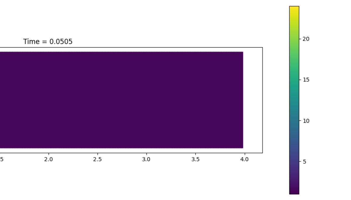
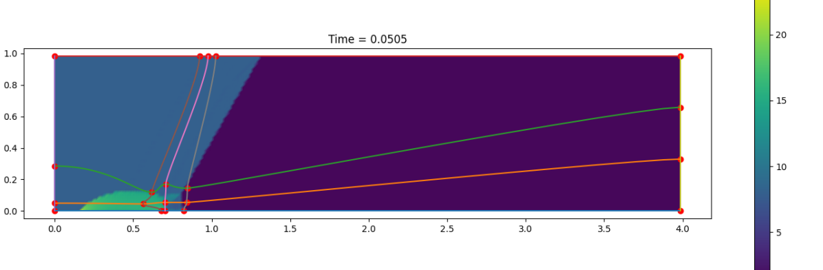
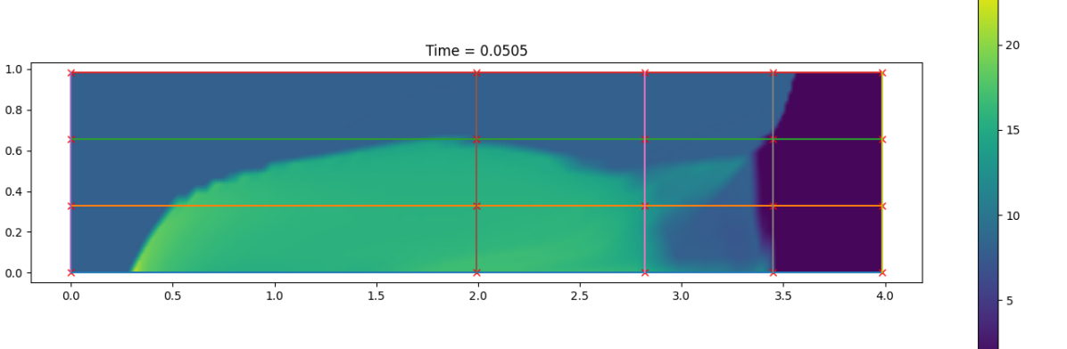
Figure 15: FOM solution for $\rho$ for DMR non parametric at times 0.05 (top), 0.15 (center) and 0.25 (bottom) in the physical domain $\Omega$ (left) and, after calibration, in the reference configuration $\mathcal{R}$ (right). We mark on the plots the control points and the Cartesian grid that links them in the reference domain and its image through $T$ on the physical one

Fig. 15 (left column) represents the FOM snapshots for the density $\rho$ at three different times of the numerical simulation; here, the same FV scheme has been employed at the FOM level on a mesh of $2400\times 600$ cells (computational time of 5 days), then downsampled to a mesh of $240\times 60$ cells to perform the offline phase (including calibration) in reasonable computational times. We retain 500 time samples in $[0,0.25]$ of which we include 45 in the training set all in $[0.02,0.2]$.

Figure 16: DMR non parametric: Error in time of reduced methods with different number $N$ of modes

Fig. 14 (left) shows the rate of decay of the eigenvalues returned by the POD on $\mathcal{M}_{\rho}$ (red): also for this test case we have a solution manifold with a slowly decaying Kolmogorov $n$–width, due to the fact that the shock moves inside $\Omega$. We therefore perform a calibration procedure, using Algorithm 1 and the 2D geometrical transformation map $T$ introduced in Section 3.2: all the details for the calibration step are summarized in Table 4. Fig. 15 (right column) shows the outcome of the calibration for the density $\rho$, at different times: here the snapshots are represented in the reference configuration $\mathcal{R}$ (computational time for forecasting the calibration points around 0.05s). With the calibration procedure, we obtain an improvement in the rate of decay of the eigenvalues, as it is shown in Figure 14 (blue line). To conclude, in Fig. 16 we show the behavior in time of the approximation error, between the FOM solution and the online solution (computational time to evaluate the NN for the ROM coefficients 0.001s), with or without calibration, according to the number $N$ of modes used. Both errors have been computed in the physical domain $\Omega$ and are defined as:

(13) $$\frac{\lvert\lvert\rho(t)-\rho_{N}(t)\rvert\rvert_{L^{2}(\Omega)}}{\lvert\lvert\rho(t)\rvert\rvert_{L^{2}(\Omega)}}\quad\text{ and }\quad\frac{\lvert\lvert\rho(t)-{\hat{\rho}}_{N}(t)\circ T^{-1}[\bm{w}^{\text{opt}}(t)]\rvert\rvert_{L^{2}(\Omega)}}{\lvert\lvert\rho(t)\rvert\rvert_{L^{2}(\Omega)}}.$$

As we see in Fig. 16, the error of the online approximation (with calibration) does not go below a certain lower bound, even increasing the number of bases. We recall that, in the calibrated setting, we are interpolating the solutions to perform the transformations: for this reason, we believe that, after a certain number $N$ of modes, the interpolation error dominates the global error, and this leads to the plateau that one can observe in the figure. We notice that with around 30 basis for the POD in the Eulerian framework we achieve errors that are comparable with the ALE solutions.

ALE $N=2$

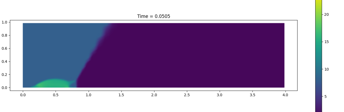
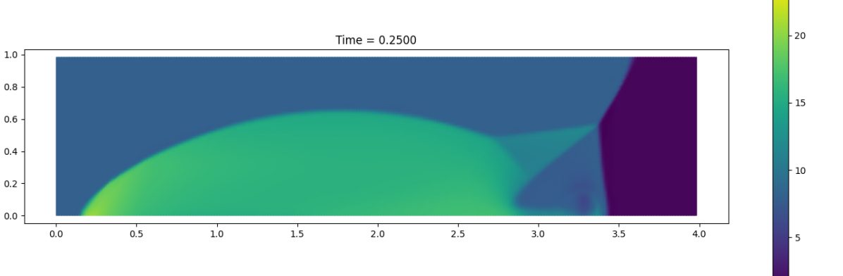
Eulerian $N=30$

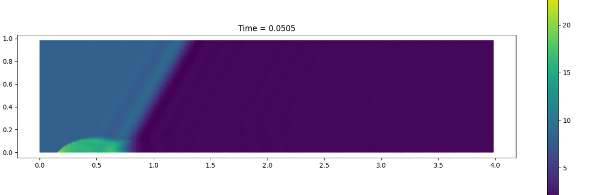
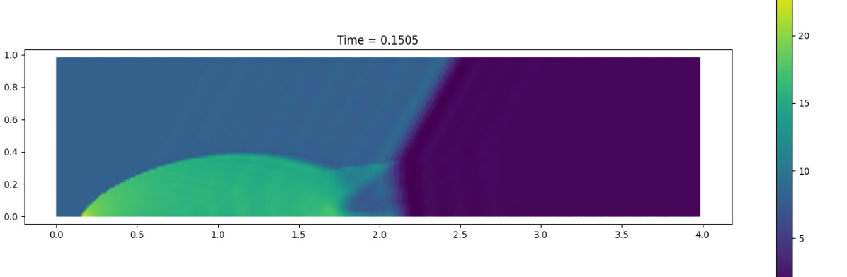
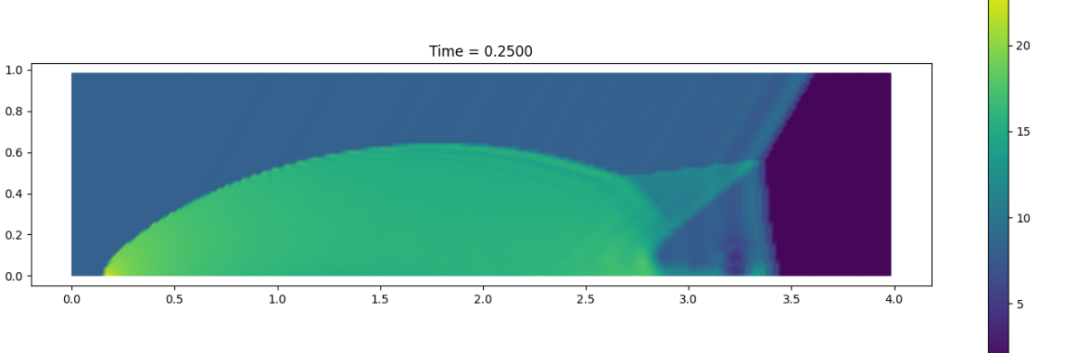
Figure 17: DMR non parametric: ROM solutions for $\rho$ in $\Omega$ at times 0.05 (top), 0.15 (center) and 0.25 (bottom). Left column: ALE ROM solution with $N=2$. Right column: Eulerian ROM solution with $N=30$

Nevertheless, the qualitatively comparison of the Eulerian and ALE approach at the ROM level with $N=2$ for the ALE approach and $N=30$ for the Eulerian approach depicted in Fig. 17 is still in favor of the ALE approach. Indeed, the Eulerian ROM shows an oscillatory behavior that deteriorates the shape of the solution, the shock position and the flat areas, which are not anymore flat. On the contrary, the ALE ROM solutions are very similar to the FOM ones and they preserve all the original features even with a much smaller reduced basis. So, even if the $L^{2}$ errors of the two approaches are comparable, the quality of the two solutions is very different.

5.4 Parametric DMR problem

In this section, we consider the parametric version of the 2D DMR problem: the physical parameter is the angle $\beta$ introduced in Section 5.3; the physical parameter interval is $\mathcal{P}_{\text{phys}}=[0.1,0.675]$, and the time interval is $[0,0.2]$. Also in this case, the FOM snapshots have been obtained with the same FV scheme, on a mesh $600\times 150$ (computational time of 2 hours each) then downsampled to $200\times 50$ for reduction of computational time of the offline phase.

Parameter $\beta=0.225$

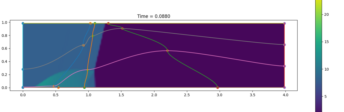
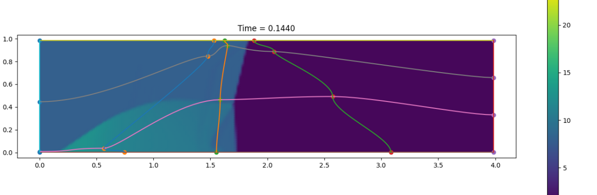
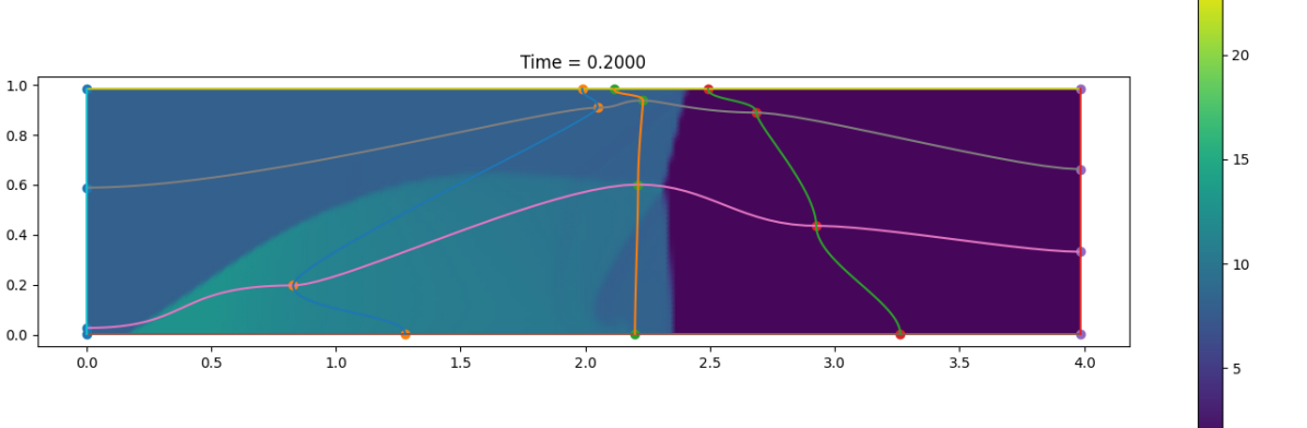
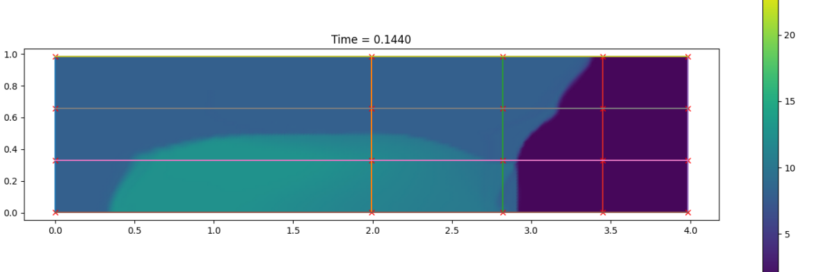
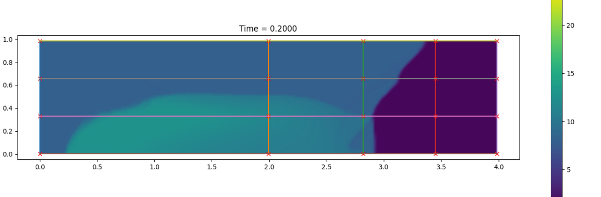
Parameter $\beta=0.675$

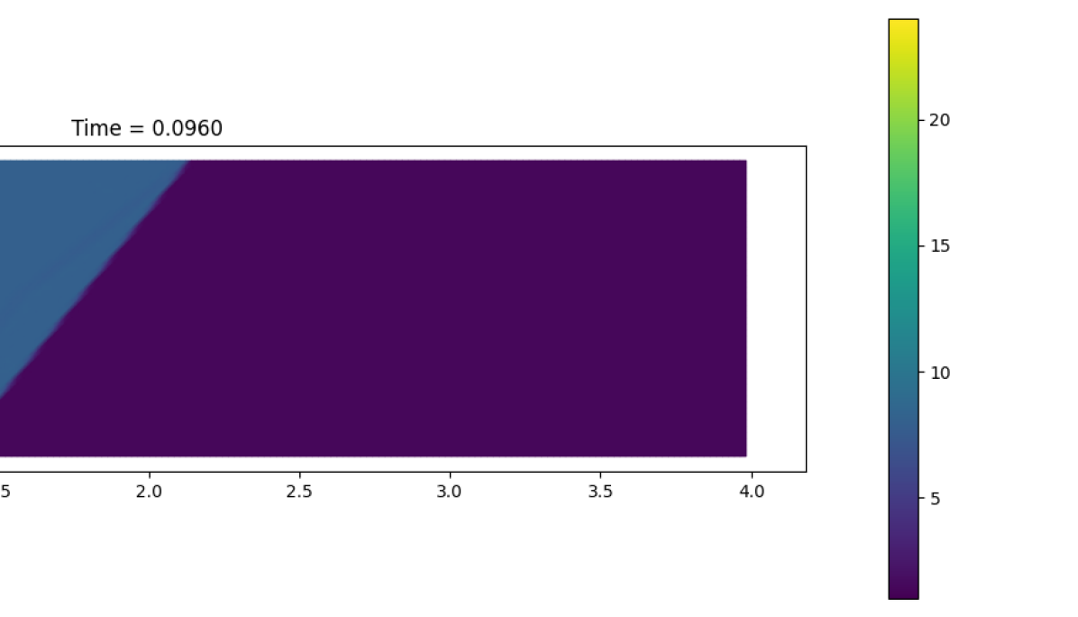
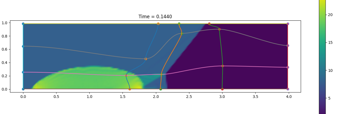
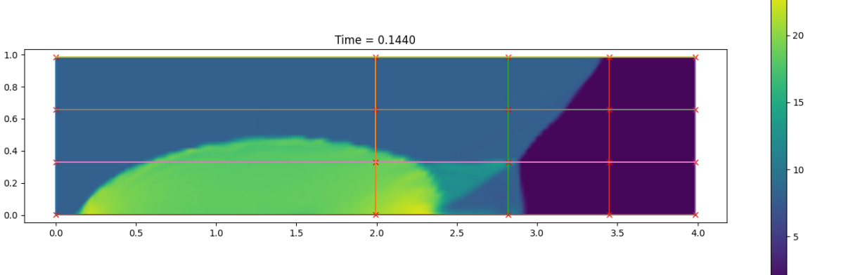
Figure 18: DMR parametric FOM solution for $\rho$ at times $t=0.096$, $t=0.148$ and $t=0.2$ (top to bottom) in the physical domain $\Omega$ (left) and, after calibration, in the reference configuration $\mathcal{R}$ (right). We mark on the plots the control points and the Cartesian grid that links them. Parameter values $\beta=0.225$ (top) and $\beta=0.675$ (bottom)

Figure 19: DMR parametric: Error in time of reduced methods with different number $N$ of modes. Parameter in test set $\beta=0.675$.

Fig. 18 shows some snapshots, for two different values of $\beta$ and at different times, before and after the calibration: all the details for the calibration procedure are summarized in Table 4. We also depicted the control points grid on the reference domain and its transformation onto the physical one, showing how the tracking of the interesting point is done and how much distortion we can get with such transformations. As we can see from Fig. 14, also in the parametric case the calibration procedure improves significantly the rate of the decay of the eigenvalues returned by the POD and hence, ultimately, the Kolmogorov $n$-width of the problem under consideration. In Fig. 19, we plot the behavior of the relative error on the physical domain, as explained in Section 5.3 in (13), varying time and for different number of modes used in the reduced spaces. On the left, we plot the error between the FOM solution and the $L^{2}$ projection onto the reduced space; on the right, we have the error obtained using the POD-NN to predict the online solution. We see that both the Eulerian and the ALE projection errors improve as we increment the number of POD modes, with the Eulerian being always much larger. In the POD-NN error, on the other side, the decay of the error is slower and it seems to stagnate at some bottleneck values, in particular for the ALE case. That is why we aim at extending this work in the future with a hyper-reduced Galerkin projection approach, to reintroduce some mathematical rigorousness hoping to decrease the online error. Finally, in Fig. 20 we represent the online solutions for $\beta=0.225$ and $\beta=0.675$, both with the Eulerian and the ALE approach with $N=6$. Similarly to what happens in the non parametric test case, the Eulerian approach struggles to reproduce the FOM solution, providing an approximation that sometimes even loses the main features (the shape of the solution, the shocks, the flat areas). On the contrary, with the ALE approach, the online approximation preserves all these features. The two parameters shown validate the ability of this ROM approach to work in strongly nonlinear parametric context, where the parameters changes the solution’s feature geometry, the values of the solution and vaguely the structure of the features. On the other hand, we remark that this approach works only for quasi-self-similar solutions, where we can recognize a similar structure along the parameter domain.

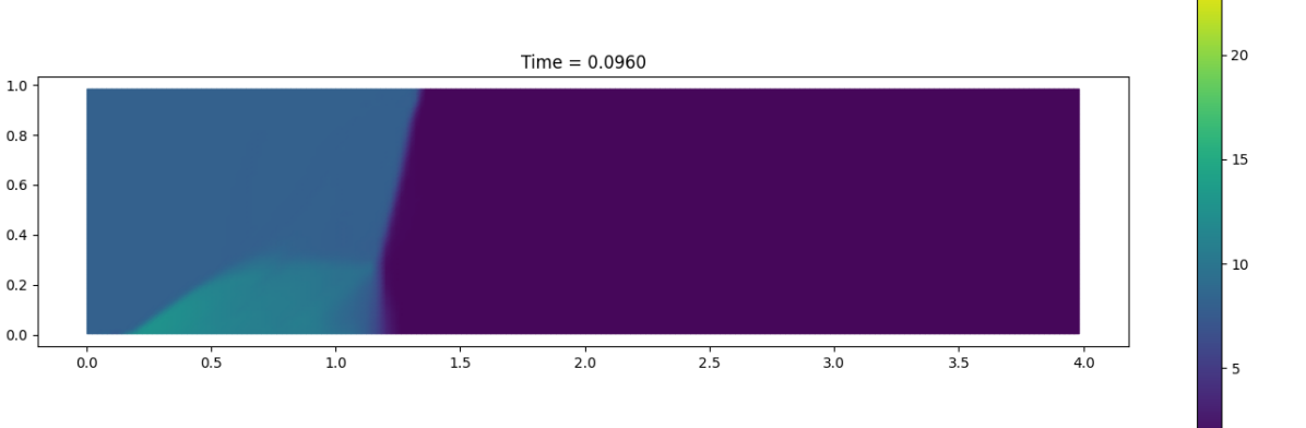
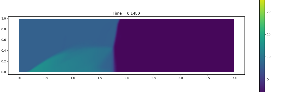
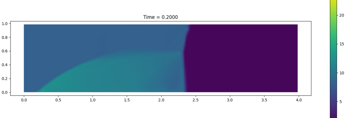
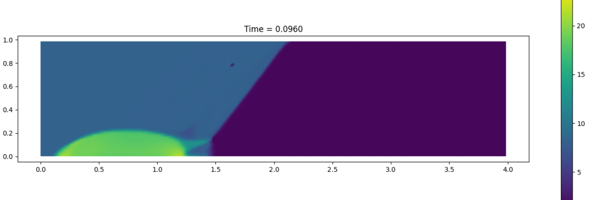
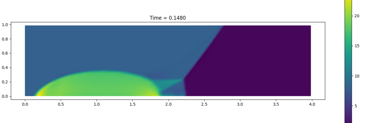
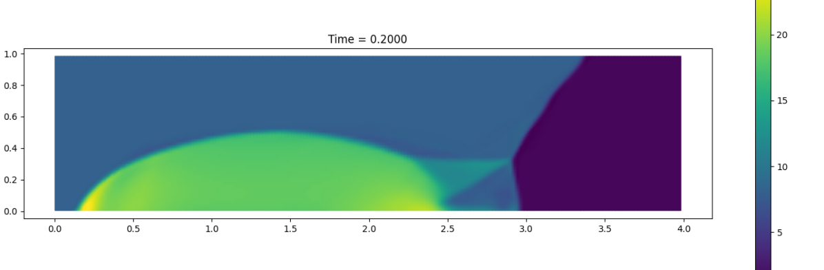
Parameter $\beta=0.225$
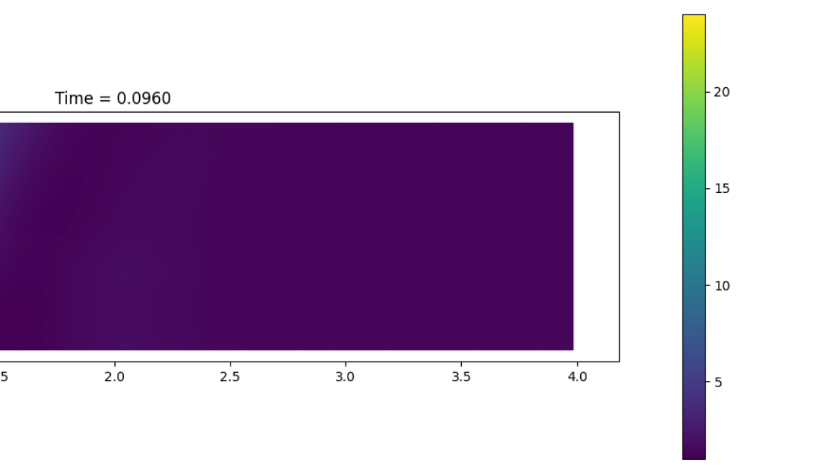
ALE POD-NN Eulerian POD-NN
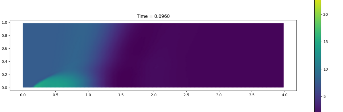
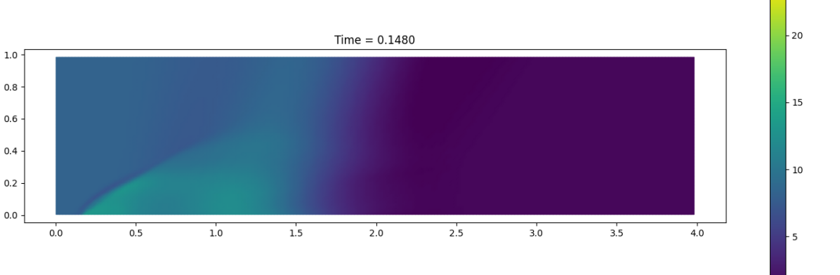
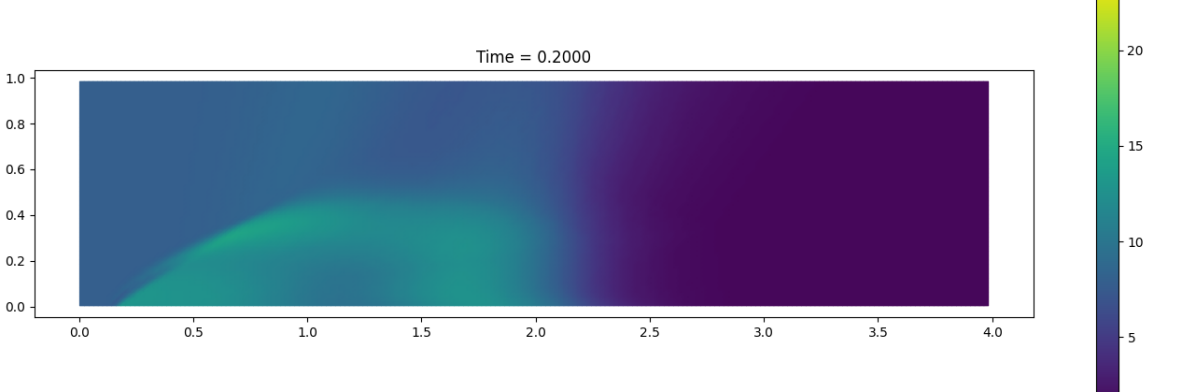
Parameter $\beta=0.675$
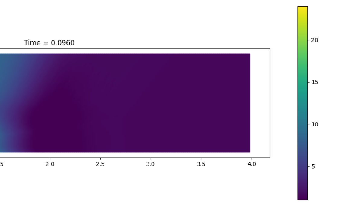
ALE POD-NN Eulerian POD-NN

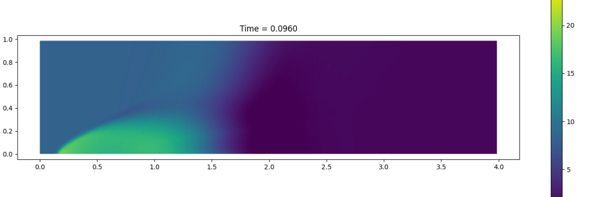
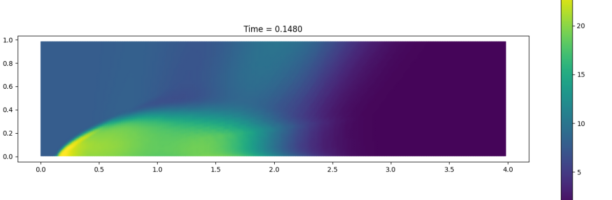
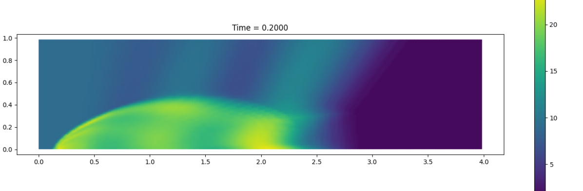
Figure 20: POD-NN solutions with $N=6$ of $\rho$ for DMR parametric at times $t=0.096$, $t=0.148$ and $t=0.2$ (top to bottom) in the physical domain $\Omega$. Left column: with the calibration of the manifold. Right column: without calibration. Parameter values $\beta=0.225$ (top) and $\beta=0.675$ (bottom)

6 Conclusions

We presented a novel, optimization-based calibration technique suited for hyperbolic conservation laws with (quasi) self-similar solutions that present multiple travelling structures, such as discontinuities. We then combined the calibration technique with an ANN based Model Order Reduction, in order to obtain an approximation setting that is able to provide satisfying results both in the non parametric and in the parametric framework, without the use of sensors or detectors of discontinuous features. To test the proposed methodology, we considered two problems of interest: the 1D Sod shock tube problem (non parametric and parametric), and the 2D DMR problem (non parametric and parametric). In all four tests, we have shown the benefits of the calibration by comparing the rate of decay of the eigenvalues returned by the PODs, showing the errors obtained with the two approaches by a POD-NN ROM and their qualitative solutions. Classical ROMs produce oscillations, smear the shocks and cannot preserve flat areas, while the presented calibrated version does, even in the context of multiple intersecting shocks and waves. The replacement of the Neural Networks with a purely ALE approach for the online system is a work in progress and a future extension of this present work. The proposed approximation setting is based on the use of piecewise cubic Hermite interpolating polynomials (or on some tensorial product of them), and works well with rectangular domains and Cartesian meshes: the extension of this approach to more complex geometries and other kinds of meshes (i.e. triangular ones) is envisioned as a future direction of this work. We also remark that, so far, we only worked with FV approximations of the full order solution. We expect to generalize the whole methodology to other discretizations.

References

- [1] R. Abgrall, D. Amsallem, and R. Crisovan, Robust model reduction by -norm minimization and approximation via dictionaries: application to nonlinear hyperbolic problems, Advanced Modeling and Simulation in Engineering Sciences, 3 (2016), p. 1, https://doi.org/10.1186/s40323-015-0055-3.
- [2] D. Amsallem, M. J. Zahr, and C. Farhat, Nonlinear model order reduction based on local reduced-order bases, International Journal for Numerical Methods in Engineering, 92 (2012), pp. 891–916, https://doi.org/10.1002/nme.4371.
- [3] N. Barral, T. Taddei, and I. Tifouti, Registration-based model reduction of parameterized PDEs with spatio-parameter adaptivity, Journal of Computational Physics, 499 (2024), p. 112727, https://doi.org/10.1016/j.jcp.2023.112727.
- [4] M. Barrault, Y. Maday, N. C. Nguyen, and A. T. Patera, An ‘empirical interpolation’ method: application to efficient reduced-basis discretization of partial differential equations, Comptes Rendus Mathematique, 339 (2004), pp. 667–672, https://doi.org/10.1016/j.crma.2004.08.006.
- [5] B. Battisti, T. Blickhan, G. Enchery, V. Ehrlacher, D. Lombardi, and O. Mula, Wasserstein model reduction approach for parametrized flow problems in porous media, ESAIM. Proceedings and Surveys, 73 (2023), p. 28, https://doi.org/10.1051/proc/202373028.
- [6] P. Benner, A. Cohen, M. Ohlberger, and K. Willcox, Model Reduction and Approximation: Theory and Algorithms, Computational Science and Engineering, Society for Industrial and Applied Mathematics, 2017.
- [7] N. Cagniart, R. Crisovan, Y. Maday, and R. Abgrall, Model Order Reduction for Hyperbolic Problems: a new framework, Hal, hal-01583224 (2017).
- [8] N. Cagniart, Y. Maday, and B. Stamm, Model order reduction for problems with large convection effects, in Contributions to Partial Differential Equations and Applications, B. N. Chetverushkin, W. Fitzgibbon, Y. Kuznetsov, P. Neittaanmäki, J. Periaux, and O. Pironneau, eds., Springer International Publishing, Cham, 2019, pp. 131–150, https://doi.org/10.1007/978-3-319-78325-3_10.
- [9] A. Cohen and R. DeVore, Kolmogorov widths under holomorfic mappings, IMA Journal of Numerical Analysis, 36 (2015), pp. 1–12, https://doi.org/10.1093/imanum/dru066.
- [10] N. Demo, M. Tezzele, and G. Rozza, EZyRB. https://mathlab.github.io/EZyRB/index.html.
- [11] A. Ferrero, T. Taddei, and L. Zhang, Registration-based model reduction of parameterized two-dimensional conservation laws, Journal of Computational Physics, 457 (2022), p. 111068, https://doi.org/10.1016/j.jcp.2022.111068.
- [12] S. Fresca, L. Dedé, and A. Manzoni, A Comprehensive Deep Learning-Based Approach to Reduced Order Modeling of Nonlinear Time-Dependent Parametrized PDEs, Journal of Scientific Computing, 87 (2021), https://doi.org/10.1007/s10915-021-01462-7.
- [13] C. Greif and K. Urban, Decay of the Kolmogorov N-width for wave problems, Applied Mathematics Letters, 96 (2019), pp. 216–222, https://doi.org/10.1016/j.aml.2019.05.013.
- [14] B. Haasdonk and M. Ohlberger, Reduced basis method for finite volume approximations of parametrized linear evolution equations, ESAIM: Mathematical Modelling and Numerical Analysis, 42 (2008), p. 277–302, https://doi.org/10.1051/m2an:2008001.
- [15] J. S. Hesthaven, G. Rozza, and B. Stamm, Certified Reduced Basis Methods for Parametrized Partial Differential Equations, SpringerBriefs in Mathematics, Springer Cham, 2016.
- [16] A. Iollo and D. Lombardi, Advection modes by optimal mass transfer, Phys. Rev. E, 89 (2014), p. 022923, https://doi.org/10.1103/PhysRevE.89.022923.
- [17] A. Iollo and T. Taddei, Mapping of coherent structures in parameterized flows by learning optimal transportation with Gaussian models, Journal of Computational Physics, 471 (2022), p. 111671, https://doi.org/10.1016/j.jcp.2022.111671.
- [18] E. N. Karatzas, F. Ballarin, and G. Rozza, Projection-based reduced order models for a cut finite element method in parametrized domains, Computers & Mathematics with Applications, 79 (2020), pp. 833–851, https://doi.org/10.1016/j.camwa.2019.08.003.
- [19] M. Khamlich, F. Pichi, and G. Rozza, Optimal Transport-inspired Deep Learning Framework for Slow-Decaying Problems: Exploiting Sinkhorn Loss and Wasserstein Kernel, arXiv preprint arXiv:2308.13840, (2023).
- [20] D. P. Kingma and J. Ba, Adam: A method for stochastic optimization, arXiv preprint arXiv:1412.6980, (2014).
- [21] K. Lee and K. T. Carlberg, Model reduction of dynamical systems on nonlinear manifolds using deep convolutional autoencoders, Journal of Computational Physics, 404 (2020), p. 108973, https://doi.org/10.1016/j.jcp.2019.108973.
- [22] J. Melenk, On n-widths for elliptic problems, Journal of Mathematical Analysis and Applications, 247 (2000), pp. 272–289, https://doi.org/10.1006/jmaa.2000.6862.
- [23] M. A. Mirhoseini and M. J. Zahr, Model reduction of convection-dominated partial differential equations via optimization-based implicit feature tracking, Journal of Computational Physics, 473 (2023), p. 111739, https://doi.org/10.1016/j.jcp.2022.111739.
- [24] R. Mojgani and M. Balajewicz, Lagrangian basis method for dimensionality reduction of convection dominated nonlinear flows, ArXiv, abs/1701.04343 (2017).
- [25] R. Mojgani, M. Balajewicz, and P. Hassanzadeh, Kolmogorov n–width and Lagrangian physics-informed neural networks: A causality-conforming manifold for convection-dominated PDEs, Computer Methods in Applied Mechanics and Engineering, 404 (2023), p. 115810, https://doi.org/10.1016/j.cma.2022.115810.
- [26] M. Nonino, F. Ballarin, G. Rozza, and Y. Maday, A reduced basis method by means of transport maps for a fluid–structure interaction problem with slowly decaying Kolmogorov -width, Advances in Computational Science and Engineering, 1 (2023), pp. 36–58, https://doi.org/10.3934/acse.2023002.
- [27] J. Núñez-de la Rosa, High-order finite volume solver for the magnetohydrodynamics equations. https://github.com/jbnunezd/fv-solver-mhd, November 2020.
- [28] M. Ohlberger and S. Rave, Nonlinear reduced basis approximation of parameterized evolution equations via the method of freezing, Comptes Rendus Mathematique, 351 (2013), pp. 901–906, https://doi.org/10.1016/j.crma.2013.10.028.
- [29] B. Peherstorfer, Model reduction for transport-dominated problems via online adaptive bases and adaptive sampling, SIAM Journal on Scientific Computing, 42 (2020), pp. A2803–A2836, https://doi.org/10.1137/19M1257275.
- [30] F. Pichi, B. Moya, and J. S. Hesthaven, A graph convolutional autoencoder approach to model order reduction for parametrized PDEs, Journal of Computational Physics, 501 (2024), p. 112762, https://doi.org/10.1016/j.jcp.2024.112762.
- [31] J. Reiss, P. Schulze, J. Sesterhenn, and V. Mehrmann, The shifted proper orthogonal decomposition: A mode decomposition for multiple transport phenomena, SIAM Journal on Scientific Computing, 40 (2018), pp. A1322–A1344, https://doi.org/10.1137/17M1140571.
- [32] T. Richter, Fluid-structure Interactions: Models, Analysis and Finite Elements, Lecture Notes in Computational Science and Engineering, Springer International Publishing, 2017.
- [33] D. Rim and K. T. Mandli, Displacement interpolation using monotone rearrangement, SIAM/ASA Journal on Uncertainty Quantification, 6 (2018), pp. 1503–1531, https://doi.org/10.1137/18M1168315.
- [34] D. Rim, S. Moe, and R. LeVeque, Transport reversal for model reduction of hyperbolic partial differential equations, SIAM/ASA Journal on Uncertainty Quantification, 6 (2018), pp. 118–150, https://doi.org/10.1137/17M1113679.
- [35] F. Romor, D. Torlo, and G. Rozza, Friedrichs’ systems discretized with the Discontinuous Galerkin method: domain decomposable model order reduction and Graph Neural Networks approximating vanishing viscosity solutions, arXiv preprint arXiv:2308.03378, (2023).
- [36] T. Taddei, A registration method for model order reduction: Data compression and geometry reduction, SIAM Journal on Scientific Computing, 42 (2020), pp. A997–A1027, https://doi.org/10.1137/19M1271270.
- [37] T. Taddei, Compositional maps for registration in complex geometries, arXiv preprint arXiv:2308.15307, (2023).
- [38] D. Torlo, Model reduction for advection dominated hyperbolic problems in an ALE framework: Offline and online phases, arXiv preprint arXiv:2003.13735, (2020).
- [39] E. Toro, Riemann Solvers and Numerical Methods for Fluid Dynamics: A Practical Introduction, Springer Berlin Heidelberg, 2013.
- [40] P. Woodward and P. Colella, The numerical simulation of two-dimensional fluid flow with strong shocks, Journal of Computational Physics, 54 (1984), pp. 115–173, https://doi.org/https://doi.org/10.1016/0021-9991(84)90142-6.
- [41] M. Yano, Discontinuous Galerkin reduced basis empirical quadrature procedure for model reduction of parametrized nonlinear conservation laws, Advances in Computational Mathematics, 45 (2019), pp. 2287–2320, https://doi.org/10.1007/s10444-019-09710-z.