Effective Computation of the Heegaard Genus of 3-Manifolds
1bab@maths.uq.edu.au 2f.thompson@uq.net.au
)
Abstract
The Heegaard genus is a fundamental invariant of 3-manifolds. However, computing the Heegaard genus of a triangulated 3-manifold is NP-hard, and while algorithms exist, little work has been done in making such an algorithm efficient and practical for implementation. Current algorithms use almost normal surfaces, which are an extension of the algorithm-friendly normal surface theory but which add considerable complexity for both running time and implementation.
Here we take a different approach: instead of working with almost normal surfaces, we give a general method of modifying the input triangulation that allows us to avoid almost normal surfaces entirely. The cost is just four new tetrahedra, and the benefit is that important surfaces that were once almost normal can be moved to the simpler setting of normal surfaces in the new triangulation. We apply this technique to the computation of Heegaard genus, where we develop algorithms and heuristics that prove successful in practice when applied to a data set of 3,000 closed hyperbolic 3-manifolds; we precisely determine the genus for at least 2,705 of these.
Keywords
3-manifolds, triangulations, normal surfaces, computational topology, Heegaard genus
Supplementary Material
Software (Source Code): github.com/FinnThompson99/heegaard
Acknowledgements
We thank the referees for their helpful comments. The second author was partially supported by the Australian Research Council (grant DP150104108).
1 Introduction
In topology, invariants are used to distinguish between different manifolds. Powerful invariants are often hard to utilise computationally, and sometimes only partial information can be calculated for them. One such example is the fundamental group, which uniquely determines hyperbolic 3-manifolds [17], but it is non-trivial to determine if two such groups are isomorphic, given their group presentations [22].
We focus on an invariant known as the Heegaard genus of a 3-manifold, which is the minimal genus of a surface (a Heegaard surface) that splits a given manifold into two handlebodies of equal genus. For example, the 3-sphere has Heegaard genus 0, and all lens spaces have Heegaard genus 1. The Heegaard genus can be used to calculate the tunnel number of a knot, which is a useful invariant in knot theory ([8], [16]).
However, computing Heegaard genus is NP-hard [1]. Algorithms of Rubinstein, Lackenby, Li, and Johannson ([19], [12], [13], [11]) provide theoretical methods, but primarily argue the existence of an algorithm; these algorithms are extremely complex to describe and theoretically extremely slow to run. Furthermore, no implementations currently exist.
These three algorithms all make use of surfaces embedded in triangulations of 3-manifolds. In particular, they use normal and almost normal surfaces, which are commonly used to certify topological properties of a manifold. Normal surfaces are described by vectors in for triangulations with tetrahedra, and can be efficiently generated using high-dimensional polytope vertex enumeration methods. However, almost normal surfaces are more complicated, requiring vectors in , which can significantly affect the running time of any algorithm using them, due to an exponential dependence on the dimension of the vector space.
Our strategy in this paper is to avoid the costs of almost normal surfaces by modifying the triangulation. Since we are solving topological problems, not combinatorial problems, we aim to retriangulate our manifolds so that important almost normal surfaces in the original triangulation (such as a surface that realises a Heegaard splitting) become normal in the new triangulation. This then allows us to attack the problem using well-studied normal surface techniques, such as the highly optimised algorithms in the software package Regina [6].
Our main tool is a new gadget, which replaces a single tetrahedron and serves to eliminate the almost normal portion of the surface. Importantly, we show that this gadget preserves the zero-efficiency of the triangulation, a property that plays a major role in making normal surface algorithms both implementable and fast ([4], [10]). We identify a class of exceptional surfaces with which this gadget cannot be used, but these exceptions are of a very specific form and are simple to analyse. For computing Heegaard genus, we show how to work around these exceptions with an alternate method for locating Heegaard splittings of this form.
Using our techniques, we are able to successfully compute the Heegaard genus of 2,705 closed, hyperbolic 3-manifolds drawn from the hyperbolic census of Hodgson and Weeks [9].
2 Preliminaries
2.1 Triangulations
To study topological objects computationally, we represent -manifolds using triangulations. These are a pairwise gluing of -dimensional simplicies along their -dimensional facets. Specifically, a 3-manifold triangulation consists of a finite number of tetrahedra that are identified (or ‘glued’) along pairs of triangular faces. Every compact 3-manifold can be represented by a triangulation [15].
Let be some arbitrary triangulation (not necessarily a simplicial complex), and consider some tetrahedron in . In the triangulation, edges, triangles (faces) and vertices of are not necessarily distinct. We use a canonical numbering of the vertices, as in Figure 1.

Let denote the triangular face constrained by vertices of tetrahedron . If a given is not a boundary facet, then this triangle is shared between (not necessarily distinct) tetrahedra and , and we may write .
2.2 (Almost) Normal Surfaces
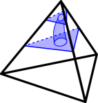
If a surface is properly embedded in a triangulation , we call it a normal surface if it meets each tetrahedron of in a collection of triangular or quadrilateral normal discs (Figure 2). In each tetrahedron, triangular discs separate one vertex from the remaining three while quadrilateral discs separate pairs of vertices. In each tetrahedron, there can be at most one of any quadrilateral type.
One such surface is a vertex linking sphere, consisting only of triangle pieces which together form a sphere (in a closed manifold) that surrounds a particular vertex in the triangulation.
Normal surfaces are represented by normal coordinates, which are vectors , notated by , where represent the number of each type in each tetrahedron, and is the number of tetrahedra in the triangulation .
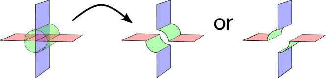
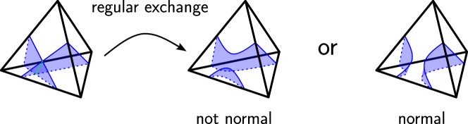
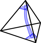
We call two surfaces locally compatible if they are able to avoid intersection in any given tetrahedron. That is, in each tetrahedron, together they use at most one type of quadrilateral piece. Locally compatible surfaces can be added using the Haken sum. If and are normal surfaces with normal coordinates , then has normal coordinates . is formed by a geometric surgery (called ‘regular exchange’), where sections of each surface are cut and glued around curves in (as in Figure 3), such that resulting pieces are normal discs (as in Figure 4).
We call a normal surface fundamental if implies or . By standard Hilbert basis arguments, any normal surface can be expressed as a sum of fundamental surfaces (which is possibly not unique).
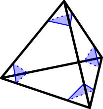
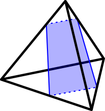
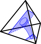
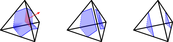
An almost normal surface is similar to a normal surface, but with the addition that it must intersect one tetrahedron in a collection of triangles and quadrilaterals, and exactly one unknotted annulus or octagon piece (see Figure 5). We shall refer to annulus pieces between quadrilaterals or triangles of the same type as parallel, and all others as non-parallel.

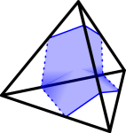
Of these almost normal pieces, there are three octagons, three parallel quadrilateral annuli, four parallel triangle annuli, six non-parallel triangle annuli and twelve triangle-quadrilateral annuli. With the four triangle and three quadrilateral normal pieces, this means that normal coordinates for almost normal surfaces are vectors in .
We call a triangulation of a closed 3-manifold zero-efficient if its only normal 2-spheres are vertex linking. Indeed, all closed, orientable, irreducible 3-manifolds (excluding , and ) can be modified to a zero-efficient triangulation, with only one vertex. A celebrated result of Jaco and Rubinstein states that if a zero-efficient triangulation of a 3-manifold has an almost normal 2-sphere, then [10].
2.3 Additional Notation
For a normal or almost normal surface in a triangulation , let represent the part of restricted to some connected sub-triangulation .
For a normal surface in a triangulation , we use to refer to the normal coordinates of restricted to some tetrahedron .
When referring to specific normal or almost normal pieces, we shall use the following.
-
•
tri_a: the link of the vertex
-
•
quad_ab/cd: the quadrilateral separating vertices from
-
•
oct_ab/cd: the octagon separating vertices from
-
•
tri_a:tri_b: the annulus connecting tri_a to tri_b, allowing .
-
•
tri_e:quad_ab/cd: the annulus connecting tri_e and quad_ab/cd, where .
2.4 Normalisation Moves
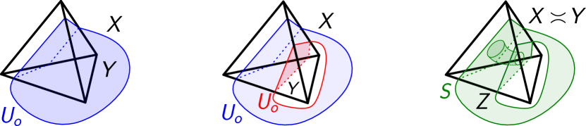
We can convert surfaces which are not yet normal into normal surfaces through a process called normalisation [10]. This is an iterative process using normalisation moves, used to convert a surface into a normal surface (possibly making changes to the topology of the surface, but which are harmless).
Two particular examples that are relevant to our work are as follows:
-
•
Compression within a tetrahedron, wherein a tubed region of the surface is cut and then ‘capped’ off with a disk. This does not change the intersection of the surface with the boundary of the tetrahedron, but reduces the Euler characteristic.
-
•
Pulling a piece across the boundary of a tetrahedron, where the surface is ‘pulled’ across an edge, reducing the number of intersections with the boundary of the tetrahedron. This possibly changes the Euler characteristic.
This second move may be used on octagon pieces in a normal surface, as seen in Figure 6 where an isotopy of oct_02/13 results in just tri_0 and tri_2.
Normalisation moves may introduce other non-normal pieces, but combinations of these moves will eventually yield a normal surface.
2.5 Implementations of Normal and Almost Normal Surfaces
Regina [6] efficiently implements data structures and algorithms for normal surfaces. However, they are still inherently exponential methods. Indeed, we have found an experimental bound on the running time of fundamental normal surface enumeration for closed hyperbolic 3-manifolds, for a triangulation with tetrahedra. See [5] for more rigorous experimental results. The number of fundamental normal surfaces for a triangulation with tetrahedra is where [3]. On the same set of closed hyperbolic 3-manifolds, we have experimentally found . See Appendix A for details. We use these experimental recordings in place of more theoretical bounds, as theoretical bounds generally represent the worst-case running times.
Almost normal surfaces have historically been motivated by 3-sphere recognition [20], which by a result of Thompson only requires use of the octagon piece [23]. In this special setting, there are techniques to normalise an almost normal surface with an octagon piece—for instance, Regina features a simple algorithm to remove octagons from an almost normal surface by modifying the triangulation using a 3-tetrahedron gadget. This technique is used in the algorithm for cutting along almost normal surfaces [18].
The more general setting that allows octagon or annulus pieces is significantly more complex to work with (with normal coordinates in ), and there are no implementations known to the authors.
2.6 Heegaard Genus
Any closed, orientable 3-manifold can be represented as where and are handlebodies (solid genus tori) with . This decomposition is called a Heegaard splitting of , and is the Heegaard surface. The Heegaard genus of is the minimal genus of all Heegaard splittings of .
All 3-manifolds with Heegaard genus 1 are classified as being either or a Lens space. Similarly, is the only 3-manifold with Heegaard genus 0 [21]. Manifolds with genus are not fully classified, and only some classes of examples are known. In general, computing the Heegaard genus of a 3-manifold is an NP-hard problem [1].
We choose to follow the techniques of Rubinstein for determining Heegaard genus [19]. For a zero-efficient triangulation of a closed, orientable -manifold, a Heegaard splitting will be of the form where is an almost normal surface with negative Euler characteristic, and is a normal surface with zero Euler characteristic [19].
To determine if a triangulation has a genus Heegaard splitting, we generate candidate almost normal surfaces and test all combinations for with Euler characteristic . That is, we cut along each candidate surface, and test whether the resulting piece/s are two handlebodies of genus , using an efficient algorithm for handlebody recognition [7]. We use algebraic properties of a given manifold to form a lower bound on genus [14]. In particular, we have where and are the number of generators of the first homology group and fundamental group of , respectively. Hence, we use as a lower bound.
3 A Gadget for Normalising Almost Normal Surfaces
Given an orientable triangulation and an almost normal surface in , we seek a way to modify into another triangulation of the same 3-manifold, so that can be expressed in using normal surfaces only, similar to the octagon gadget (see Section 2.5). As almost normal pieces only appear within a single tetrahedron, we desire a small triangulation that we may substitute for a tetrahedron. That is, we desire an orientable triangulation that is homeomorphic to the 3-ball (), with four vertices and four boundary faces. We shall call such a triangulation the gadget.
3.1 A General Gadget Construction
Suppose that is a triangulation such that , with four vertices and four boundary faces, arranged to form the boundary of a tetrahedron. We define to represent the boundary facet that is constrained by vertices of the gadget . Then, the boundary of is isomorphic to the boundary of a single tetrahedron, and so we can effectively ‘replace’ a tetrahedron in with as follows.
We define to be the resulting triangulation formed by removing from , and gluing in its place according to the permutation mapping vertices of to by . This operation is simply un-gluing each face of from , then gluing the corresponding boundary face of in its place (as indicated in Figure 7) where

If any pair of faces of are glued to each other, for example , then we glue the boundary faces of the gadget accordingly, such as .
3.2 Gadget Requirements
Here, we discuss motivations behind a choice for the gadget. As discussed, we assume that has isomorphic boundary to the boundary of a tetrahedron, and is itself homeomorphic to . Now, consider some gluing of the gadget into a triangulation to form . As and , does not modify topological properties of the triangulation, , in which it is placed. In addition, we desire the following.
-
•
If is zero-efficient, then is also zero-efficient, aside from simple exceptions.
-
•
There must be a well-defined choice of normal surfaces in that each correspond to one of the four triangular or three quadrilateral pieces of a normal surface in . Similarly, there must be a well-defined choice of an octagon piece, and some annulus pieces (discussed in Lemma 3.6), such that local compatibility of these surfaces matches the local compatibility of (almost) normal pieces. For example, we require that the triangle pieces in are compatible with all other pieces.
This means that if is a normal surface in , then there must exist some normal surface in with identical normal coordinates outside of /, where additionally is isotopic to . Similarly, the normal surfaces of chosen to represent (almost) normal pieces should be sufficient to construct any almost normal surface of , aside from some manageable exceptions. That is, if a surface has an almost normal piece in , then for some (possibly distinct) tetrahedron and some permutation , there must exist a normal surface in where is isotopic to .
3.3 Choice of the Gadget
The requirements that the boundary of must be isomorphic to the boundary of a tetrahedron, and that is homeomorphic to , are both targeted using Regina’s tricensus command, which generates a list of triangulations satisfying given conditions.
To ensure that the chosen triangulation would have surfaces equivalent to annulus or octagon pieces, a search of the fundamental normal surfaces was conducted. Examining the boundary components of each surface for each triangulation yielded a candidate for our gadget .
We now denote the 5-tetrahedron triangulation with isomorphism signature (a compact code used to uniquely generate triangulations in Regina) ‘fHLMabddeaaaa’ by , or the gadget.
In version 7.x of Regina, the command Triangulation3(‘fHLMabddeaaaa’) can be used to reconstruct our gadget. Table 1 provides the gluing instructions for pairs of faces of the five tetrahedra. Here, ‘Face ’ refers to the triangular face that meets vertices , and represents face of tetrahedron .
| Tetrahedron | Face 012 | Face 013 | Face 023 | Face 123 |
|---|---|---|---|---|
| 0 | 2 (012) | 1 (013) | 1 (123) | |
| 1 | 3 (012) | 0 (013) | 3 (023) | 0 (123) |
| 2 | 0 (012) | 4 (013) | 4 (023) | 3 (123) |
| 3 | 1 (012) | 1 (023) | 2 (123) | |
| 4 | 2 (013) | 2 (023) |
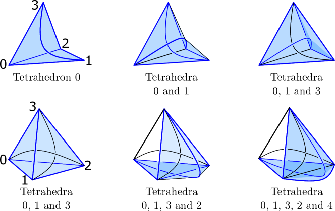
Alternatively, Figure 8 provides a geometric description of the construction of the gadget.
The fundamental normal surfaces of are detailed below, along with their index when generated by Regina. See Table 3 of Appendix B for details of their normal coordinates. Boundary types are determined by observing the polygonal boundary of each surface in the gadget, and determining its shape (e.g triangular boundaries have three sides).
| # bdry | Euler char. | Shape | Boundary types | Index |
| 1 | -1 | One-punctured torus | Quad | 0, 3 |
| 1 | Octagon | Oct | 17, 18 | |
| Triangle | Tri | 7, 8, 10, 13 | ||
| Quadrilateral | Quad | 2, 5, 6, 11, 12 | ||
| 2 | 0 | Annulus (non-parallel triangles) | Two tri | 1, 4, 16, 19 |
| Annulus (quadrilateral, triangle) | Quad, tri | 9, 27 | ||
| Annulus | Oct, tri | 15, 26 | ||
| 3 | -1 | Three-punctured sphere | Three tri | 14, 25 |
| Three-punctured sphere | Quad, two tri | 23, 24, 28 | ||
| Three-punctured sphere | Oct, two tri | 22 | ||
| -3 | Three-punctured torus | Quad, two tri | 20 | |
| 4 | -2 | Four-punctured sphere | Four tri | 21 |
We refer to the surface with index i by sf_i. Note that rows where multiple indexes are listed simply represent instances of different orientations of the same surface.
Next, we explore the surfaces in that correspond to normal and almost normal pieces in a single tetrahedron .
Triangles
The four triangular disc surfaces (sf_7, sf_8, sf_10, sf_13) are vertex links in , and are hence composed of triangle pieces only. These are isotopic to the four triangular pieces we consider for a normal surface. Due to this, we introduce the following more insightful names,
Quadrilaterals
The three quadrilateral pieces in are each isotopic to at least one of the quadrilateral surfaces in the gadget (sf_2, sf_5, sf_6, sf_11, sf_12).
Surfaces sf_2 and sf_12 both represent quad_03/12. However, surface sf_12 is not locally compatible with the annulus tri_3:quad_03/12 (that is, sf_9) – this is undesired, so we choose surface sf_2 to represent this quadrilateral.
Similarly, surfaces sf_5 and sf_11 both represent quad_02/13. Without loss of generality, we arbitrarily choose surface sf_5 to represent this quadrilateral. So, we introduce the following names,
Corollary 3.1.
With this construction, for a normal surface in a triangulation , we can choose a normal surface in where in , has normal coordinates
where are the normal coordinates of in . Hence, is isotopic to .
Annuli and Octagons
Among the normal surfaces in the gadget, we also have candidates for almost normal pieces. Namely, sf_17 and sf_18 are both discs with octagonal boundary, and we declare that
Finally, with the presence of four different annulus pieces between non-parallel triangles, and two of triangle-quadrilateral type, we choose
Note that parallel annuli are missing from , this will be discussed later.
3.4 Verifying Requirements
With the normal and almost normal pieces of the gadget identified, we now show that our choice of satisfies the properties discussed in Section 3.2.
Observation 3.2.
The sum of any two fundamental normal surfaces in can be expressed as the sum of pairwise disjoint fundamental surfaces. This can be verified in Regina.
Note that this is not true for all triangulations, as in general the connected components of a normal surface may include non-fundamental surfaces.
Lemma 3.3.
Any normal surface in the gadget can be expressed as a sum of pairwise disjoint fundamental normal surfaces.
The approach we take is to express any normal surface as the sum of connected fundamental surfaces, by repeatedly using Observation 3.2 on pairs of intersecting surfaces, allowing us to rewrite this surface in a way that has fewer intersections between its summands.
Proof.
Let be a normal surface in the gadget, where each is a fundamental normal surface (not necessarily distinct) and consider the set . Let represent the total number of intersection curves between these surfaces, noting that surfaces intersect transversely. In particular, we may ‘push’ components of so that no two intersection curves meet within .
Now, take two surfaces that are not disjoint. By Observation 3.2, in the Haken sum of and , we find where are pairwise disjoint fundamental normal surfaces. Consider some curve in . Within a small open regular neighbourhood of , , a regular exchange is performed as in Figure 3, such that all intersections resolve to normal discs, as in Figure 4. This decreases the number of intersections by for each .
We have verified that resolving the intersections of does not increase . Now, we must check that any intersections with any additional surfaces are not created.
Take some surface that intersects and/or . Each curve in or is outside of the regions , so evaluating does not create any new intersections between and any component . In fact, the sets of intersection curves are equal. So, is strictly decreasing.
We may continue this process again for some new pair of intersecting, fundamental surfaces, until and we have a collection of disjoint, fundamental surfaces. ∎
Theorem 3.4.
Let be a zero-efficient triangulation of a 3-manifold which is not , or . Remove some tetrahedron from and replace it with according to some permutation . Then the resulting triangulation is also zero-efficient.
Proof.
According to Proposition 5.1 of [10], because is zero-efficient and not , or , it is a one-vertex triangulation. As and have the same number of vertices, is a one-vertex triangulation.
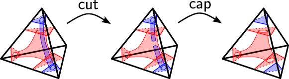
So, we suppose that is zero-efficient, but is not. That is, suppose that has some non-vertex-linking normal 2-sphere . By Lemma 3.3, the connected components of are all fundamental normal surfaces as described in Table 2 – excluding sf_0, sf_3, sf_20, which have genus . Now, consider embedding into to form the surface , so that in tetrahedron we have that is isotopic to . This is not necessarily a normal surface, so we attempt to normalise it. As is a sphere, any tubed piece within may be cut and ‘capped’ (see Section 2.4), cutting into two spheres. In particular, we find an inner-most tube in , and cut and cap it as in Figure 9.
As we repeat this process, we form , a collection of spheres, with . The components of are triangles, plus possibly either octagons or quadrilaterals (but not both as they are not locally compatible).
If has one or more octagon piece, then we normalise all but one octagon by pushing them towards adjacent tetrahedra (see Figure 6 in Section 2.4). Now, since exactly one octagon remains, has a component that is an almost normal sphere in . From Proposition 5.12 of [10], this means must be – but this contradicts our assumptions about .
Now, if has quadrilaterals but no octagons, then it has a component that is a normal 2-sphere in which is not vertex linking. This contradicts being zero-efficient.
Finally, consider the case where has only triangular pieces. As we assumed that is not vertex linking, then must have had at least one copy of an annulus between triangles. But, as is a one-vertex triangulation, this means that had genus , as each tube essentially adds a handle to a vertex linking sphere formed from the remaining triangles. But, then is not a sphere, so we again find a contradiction.
In each case, we have reached a contradiction to the assumption that is not zero-efficient. Hence, we can conclude that the gadget preserves zero-efficiency.
∎
Now, we address the parallel annulus types that are not captured by the gadget, and show why this exceptional case is harmless for algorithms such as computing Heegaard genus.
Observation 3.5.
Suppose is an almost normal surface in some closed triangulation . If the almost normal piece in is an annulus in tetrahedron , then on any face of that intersects the annulus twice, the annulus may be isotoped (‘pushed across’) to the adjacent tetrahedron.
For example, consider such a case in Figure 10.
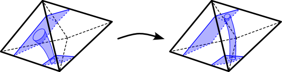
The normal discs in the adjacent tetrahedron need not be the same type, as in Figure 10.
Whether pairs of boundary curves constrained to the shared face are parallel determines what annulus piece may appear in this adjacent tetrahedron. Which face the tube is pushed towards determines which annulus may appear in the adjacent tetrahedron.
Lemma 3.6.
Let be a connected, almost normal surface in a closed, orientable triangulation (which is not the 3-sphere). Suppose it has an annulus piece of parallel triangle or quadrilateral type in some tetrahedron . Then, one of the following holds:
-
1.
is isotopic to an almost normal surface with a non-parallel boundary type annulus in some (possibly different) tetrahedron ;
-
2.
does not represent a minimal Heegaard splitting;
-
3.
is the orientable double cover of some non-orientable surface with a tube connecting the two sheets that cover some local region of .
Proof.
Suppose we have a surface with an annulus of either parallel-triangle or parallel-quadrilateral type. We attempt to push the tube from tetrahedron to tetrahedron until reaching a non-parallel annulus type. If successful, this proves Case 1.
If a non-parallel piece cannot be found, then our surface must either be two parallel copies of an orientable surface , or the orientable double cover of a non-orientable surface , in both cases with a tube connecting its two sheets. The non-orientable case is simply Case 3, which will be discussed after the proof.
Suppose that realises a Heegaard splitting of genus and therefore has Euler characteristic .
If where is orientable and separating, then has Euler characteristic and splits the triangulation into 3-manifolds and where . Refer to Figure 11. Now, consider the 3-manifold bounded by , wedged between the two copies of . As for the Heegaard splitting , has genus . To the other side of is the 3-manifold , which is connected to by a solid tube. As is a Heegaard splitting, must also be a handlebody of genus . But, then and are both handlebodies of genus (because they are both bounded individually by the genus surface ), so is a Heegaard splitting of genus . Hence, is not a minimal Heegaard splitting (unless , but is not the 3-sphere).
Finally, if but is non-separating, then cutting along yields a 3-manifold with a properly embedded disc (slicing through the tube) that separates but not . Therefore is not a handlebody and is not a Heegaard splitting, giving us Case 2.
∎
Consider Case 3 of the previous lemma. We abuse notation and let represent the orientable double cover of with a tube connecting its two sheets. Cutting the triangulation along yields the 3-manifold with . Since cuts into two handlebodies of genus , it follows that is just one of these handlebodies with one of its handles cut. That is, is a handlebody with genus . Such a case can be detected by searching for surfaces with Euler characteristic which cut the triangulation into one genus handlebody.
Corollary 3.7.
For an almost normal surface that realises a minimal Heegaard splitting of a triangulation , one of the following holds:
-
1.
There exists a gluing of the gadget into to form for some permutation and some tetrahedron , and there exists a normal surface in that is isotopic to ;
- 2.
Proof.
Suppose that is an almost normal surface in a triangulation , with its almost normal piece in tetrahedron .
There are twelve rotational symmetries of a tetrahedron (twelve even permutations of its vertices), and hence twelve possible triangulations that may be formed for each tetrahedron.
We may transform the coordinates of the normal pieces as in Corollary 3.1.
If the almost normal piece of is an annulus between parallel triangles or quadrilaterals, then we attempt to push this tube across the tetrahedra until reaching a non-parallel annulus piece, and apply the gadget accordingly. If this is unsuccessful, then must be the orientable double cover of some non-orientable normal surface with a tube connecting its two sheets, as in Case 3 of Lemma 3.6. Then, to determine if is a genus Heegaard splitting, simply cut along and check, via the algorithm for handlebody recognition [7], whether the resulting manifold is a genus handlebody.
Now, if the almost normal piece of is an octagon or a non-parallel annulus piece, then we seek to construct a surface in for some permutation of the vertices of into , .
As the gadget has two distinct triangle-quadrilateral annulus pieces of a total possible twelve, each permutation of the gadget can represent two distinct annuli of this type. Hence, we only need to try six possible permutations. We choose the following,
This choice of permutation allows us to ‘rotate’ the required octagon or annulus piece of into the same position as the one in . Refer to Appendix C for the specific choices of individual almost normal pieces.
∎
3.5 Implementations
In practice, as there is no current implementation of annulus pieces in Regina, we cannot directly normalise an almost normal surface using the gadget. Instead, we need to consider all normal surfaces from all possible triangulations resulting from gluing the gadget into any tetrahedron.
With the gadget, Heegaard splittings can now always be represented by normal surfaces. However, these surfaces are not necessarily fundamental. Therefore we use the gadget to generate a set of candidate surfaces for each potential value of genus; this set will be finite, due to Euler characteristic being additive under Haken sum. We discuss this process further in Section 4.
3.5.1 Method 1: Generating All Surfaces
For each tetrahedron in a triangulation , form for the six distinct permutations (see the proof of Corollary 3.7), and then generate all fundamental normal surfaces in it. For a triangulation with tetrahedra, this means sets of normal surfaces must be enumerated. This represents almost normal surfaces that may be embedded in , as well as many others (which use surfaces of the gadget that are not tubes, octagons, triangles or quadrilaterals).
Denote the running time for generating normal surfaces for a triangulation with tetrahedra by , and let represent the number of normal surfaces for such a triangulation. From Section 2.5, and . Suppose that the running time of the algorithm to check if a surface is a Heegaard splitting has running time . Then, to generate and test each surface in the triangulations, we find a running time on the order of .
3.5.2 Method 2: Constructing Each Annulus
Alternatively, we have developed a method to form the necessary set of almost normal surfaces using an existing set of fundamental normal surfaces for the base triangulation.
Let be the set of fundamental normal surfaces for a triangulation . For each surface , we form a set of almost normal surfaces with an annulus piece between triangles and/or quadrilaterals in as follows. For each tetrahedron , if has at least two triangles on different vertices, then we consider the surface with an annulus between two of these triangles. Similarly, if has at least one triangle and at least one quadrilateral, we consider the surface with an annulus between these. In either case, we determine which annulus type from the gadget is necessary, and under which permutation, and construct the new surface within . As we begin with a set of normal surfaces (that is, they are not already ‘tubed’), when we form the equivalent surface in , we must add the coordinates for the annulus piece to the coordinates for each triangle or quadrilateral excluding those corresponding to the boundaries of the annulus.
For example, in Figure 12, has coordinates and supports several annulus types, such as one connecting a triangle to its quadrilateral. Using the identity permutation, we find that gives us the annulus between tri_3:quad_03/12. Then, the remaining triangle pieces are represented using and .
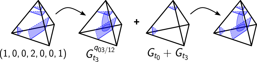
A complete guide to our choice of permutations and coordinates is given in Appendix C.
Now, using the same results from Section 2.5, the running time for this method is on the order of , as there are at most six annulus types that could exist in any given tetrahedron.
Performance Comparison
In our discussion of the two methods, we found and , where is the time to test if a given surface is a Heegaard splitting. Asymptotically , and so we expect method 2 to be significantly faster than method 1.
Generating All Surfaces with Method 2
In Method 2 (Section 3.5.2), we described how a non-parallel annulus of an almost normal surface can be converted into a normal surface using the gadget. Here, we justify that this method produces all the candidate almost normal surfaces that may represent a minimal Heegaard splitting. First, suppose that almost normal surfaces with octagon pieces have been considered already (i.e. have been tested as Heegaard splittings). Now, any almost normal surface with an annulus piece has such an annulus ‘tubing’ together two triangles and/or quadrilaterals.
Suppose is an orientable fundamental almost normal surface with Euler characteristic , with a non-parallel annulus in some tetrahedron . Let be the surface generated by cutting and capping the annulus. Of course, and is a normal surface, but is not necessarily fundamental, so for some fundamental normal surfaces . The annulus of either connects two components in of a particular , or connects two components between and for . We can generate all tubings of to itself by constructing tubes as in Section 3.5.2. Similarly, we can generate tubings of .
Now, if has a parallel annulus piece, then either it is of the type of Case 3 in Lemma 3.6, or will not represent a minimal Heegaard splitting, or it is isotopic to some with a non-parallel annulus.
In practice, this results in the following method for detecting a splitting of genus .
-
1.
Generate the set of all fundamental almost normal surfaces of a triangulation in Regina, test if those with genus are Heegaard splittings. If not, generate the set of fundamental normal surfaces, .
-
2.
For each tetrahedron, for each orientable surface of genus in , form all tubings.
-
3.
For each tetrahedron, for each set of locally compatible surfaces in whose Euler characteristics sum to , form all tubings.
-
4.
Test all tubed surfaces as Heegaard splittings.
Note that constructing a tube increases the Euler characteristic of a surface by 2, which is equivalent to increasing the genus of a connected surface by 1.
4 Computing Heegaard Genus
As discussed in Section 2.6, a result of Rubinstein declares that Heegaard splittings are given by where is almost normal, is normal, and [19]. So, to determine if a triangulation has a genus Heegaard splitting, all such surfaces where must be tested as splittings. Furthermore, we know that every summand of must have negative Euler characteristic, and every summand of has zero Euler characteristic. Hence, there are finitely many cases to consider of as their Euler characteristic must represent an integer partition of . We can generate these using normal and almost normal surfaces in Regina with octagon pieces, or by constructing tubed surfaces as in Section 3.5.2.
For the torus piece , as Euler characteristic is additive under Haken sum, this could theoretically require an unbounded number of different sums of tori. However, from Lemma 5.1 of [2], we know that if is a normal surface and is an edge-linking torus, then is either disconnected or is isotopic to , so need not be considered in summands of . Tentatively and naively, we therefore consider splittings as only. If there are non-edge-linking tori present, this means we may not see our splitting, and so in such settings we can only form an upper bound on the genus. Experimentally, edge-linking tori do form the majority of tori in the cases we have tested, and in those cases that remain, we can attempt to form a lower bound using algebraic techniques as in Section 2.6.
We have tested this approach on all orientable triangulations in the closed hyperbolic census of Hodgson and Weeks (in [9]) – all of which are zero-efficient. We first search for a genus 2 splitting, and if one does not exist, search for a genus 3 splitting (then 4, etc). Of the 3,000 triangulations in this census, 44 had , and genus 3 splittings were found. Then, 2,661 had , and genus 2 splittings were found. For each of the remaining 295, an exhaustive search of genus 2 surfaces (without tori) found no splittings, but genus 3 splittings were found. In these 295 cases, we cannot guarantee they have genus 3, but merely provide an informed upper bound.
References
- [1] David Bachman, Ryan Derby-Talbot, and Eric Sedgwick. Computing Heegaard genus is NP-hard. In A journey through discrete mathematics, pages 59–87. Springer, Cham, 2017.
- [2] Birch Bryant, William Jaco, and J. Hyam Rubinstein. Efficient triangulations and boundary slopes. Topology Appl., 297:Paper No. 107689, 18, 2021. doi:10.1016/j.topol.2021.107689.
- [3] Benjamin A. Burton. The complexity of the normal surface solution space. In Computational geometry (SCG’10), pages 201–209. ACM, New York, 2010. doi:10.1145/1810959.1810995.
- [4] Benjamin A. Burton. A new approach to crushing 3-manifold triangulations. In Computational geometry (SoCG’13), pages 415–423. ACM, New York, 2013. doi:10.1145/2462356.2462409.
- [5] Benjamin A. Burton. Enumerating fundamental normal surfaces: Algorithms, experiments and invariants. In ALENEX 2014: Proceedings of the Sixteenth Workshop on Algorithm Engineering and Experiments, pages 112–124. SIAM, 2014.
- [6] Benjamin A. Burton, Ryan Budney, William Pettersson, et al. Regina: Software for low-dimensional topology. http://regina-normal.github.io/, 1999–2023.
- [7] Benjamin A. Burton and Alexander He. Finding large counterexamples by selectively exploring the Pachner graph. In 39th International Symposium on Computational Geometry, volume 258 of LIPIcs. Leibniz Int. Proc. Inform., pages Art. No. 21, 16. Schloss Dagstuhl. Leibniz-Zent. Inform., Wadern, 2023. doi:10.4230/lipics.socg.2023.21.
- [8] Bradd Clark. The Heegaard genus of manifolds obtained by surgery on links and knots. Internat. J. Math. Math. Sci., 3(3):583–589, 1980. doi:10.1155/S0161171280000440.
- [9] Craig D. Hodgson and Jeffrey R. Weeks. Symmetries, isometries and length spectra of closed hyperbolic three-manifolds. Experiment. Math., 3(4):261–274, 1994. URL: http://projecteuclid.org/euclid.em/1048515809.
- [10] William Jaco and J. Hyam Rubinstein. -efficient triangulations of 3-manifolds. J. Differential Geom., 65(1):61–168, 2003. URL: http://projecteuclid.org/euclid.jdg/1090503053.
- [11] Klaus Johannson. Heegaard surfaces in Haken -manifolds. Bull. Amer. Math. Soc. (N.S.), 23(1):91–98, 1990. doi:10.1090/S0273-0979-1990-15910-5.
- [12] Marc Lackenby. An algorithm to determine the Heegaard genus of simple 3-manifolds with nonempty boundary. Algebr. Geom. Topol., 8(2):911–934, 2008. doi:10.2140/agt.2008.8.911.
- [13] Tao Li. An algorithm to determine the Heegaard genus of a 3-manifold. Geom. Topol., 15(2):1029–1106, 2011. doi:10.2140/gt.2011.15.1029.
- [14] Tao Li. Rank and genus of 3-manifolds. J. Amer. Math. Soc., 26(3):777–829, 2013. doi:10.1090/S0894-0347-2013-00767-5.
- [15] Edwin E. Moise. Affine structures in -manifolds. V. The triangulation theorem and Hauptvermutung. Ann. of Math. (2), 56:96–114, 1952. doi:10.2307/1969769.
- [16] Kanji Morimoto. On Heegaard splittings of knot exteriors with tunnel number degenerations. Topology Appl., 196:719–728, 2015. doi:10.1016/j.topol.2015.05.042.
- [17] G. D. Mostow. Quasi-conformal mappings in -space and the rigidity of hyperbolic space forms. Inst. Hautes Études Sci. Publ. Math., (34):53–104, 1968. URL: http://www.numdam.org/item?id=PMIHES_1968__34__53_0.
- [18] William Pettersson and Benjamin A. Burton. ”Normalise” AlmostNormal surfaces, 2017. URL: https://github.com/regina-normal/regina/issues/33.
- [19] J. H. Rubinstein. Polyhedral minimal surfaces, Heegaard splittings and decision problems for -dimensional manifolds. In Geometric topology (Athens, GA, 1993), volume 2 of AMS/IP Stud. Adv. Math., pages 1–20. Amer. Math. Soc., Providence, RI, 1997. doi:10.1090/amsip/002.1/01.
- [20] Joachim H. Rubinstein. An algorithm to recognize the -sphere. In Proceedings of the International Congress of Mathematicians, Vol. 1, 2 (Zürich, 1994), pages 601–611. Birkhäuser, Basel, 1995.
- [21] Nikolai Saveliev. Lectures on the topology of 3-manifolds. De Gruyter Textbook. Walter de Gruyter & Co., Berlin, revised edition, 2012. An introduction to the Casson invariant.
- [22] Z. Sela. The isomorphism problem for hyperbolic groups. I. Ann. of Math. (2), 141(2):217–283, 1995. doi:10.2307/2118520.
- [23] Abigail Thompson. Thin position and the recognition problem for . Math. Res. Lett., 1(5):613–630, 1994. doi:10.4310/MRL.1994.v1.n5.a9.
- [24] Pauli Virtanen, Ralf Gommers, Travis E. Oliphant, Matt Haberland, Tyler Reddy, David Cournapeau, Evgeni Burovski, Pearu Peterson, Warren Weckesser, Jonathan Bright, Stéfan J. van der Walt, Matthew Brett, Joshua Wilson, K. Jarrod Millman, Nikolay Mayorov, Andrew R. J. Nelson, Eric Jones, Robert Kern, Eric Larson, C J Carey, İlhan Polat, Yu Feng, Eric W. Moore, Jake VanderPlas, Denis Laxalde, Josef Perktold, Robert Cimrman, Ian Henriksen, E. A. Quintero, Charles R. Harris, Anne M. Archibald, Antônio H. Ribeiro, Fabian Pedregosa, Paul van Mulbregt, and SciPy 1.0 Contributors. SciPy 1.0: Fundamental Algorithms for Scientific Computing in Python. Nature Methods, 17:261–272, 2020. doi:10.1038/s41592-019-0686-2.
Appendix A Running Time Computations
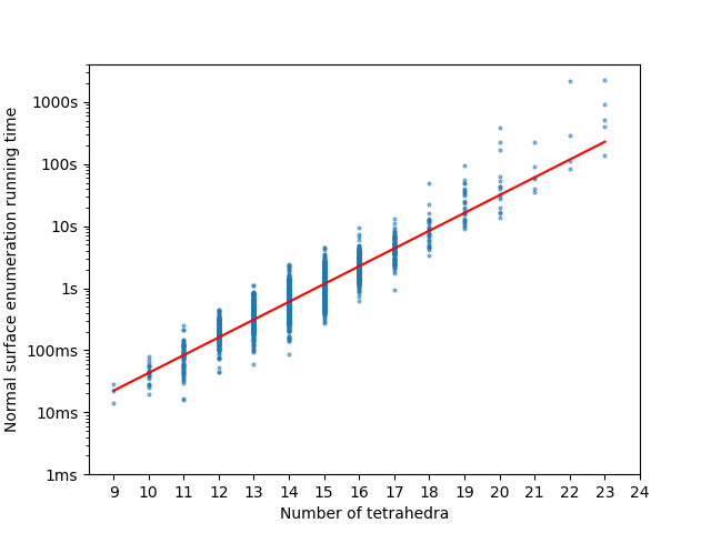
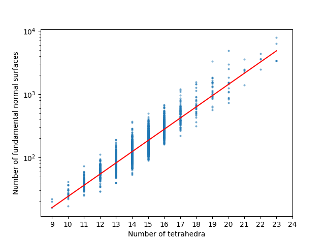
Of the first 3000 triangulations in the Hodgson-Weeks Closed Hyperbolic Census in Regina, fundamental normal surfaces were generated for the 2974 triangulations with at most 23 tetrahedra. The number of surfaces and enumeration time were recorded. These tests were run on an 8-core CPU with 16GB RAM.
Using curve_fit in SciPy [24], we fit linear models to and where is the number of tetrahedra, is the running time and is the number of normal surfaces. We found with for the enumeration time, and with for the number of surfaces. Equivalently, and . By this, we may estimate that and .
Appendix B Fundamental Normal Surfaces of the Gadget
The coordinates of the surfaces introduced in Table 2 are detailed below. The coordinates and order of the surfaces are as produced in version 7.3 of Regina, for the triangulation with isomorphism signature ‘fHLMabddeaaaa’. To replicate these surfaces in Regina, use the command
NormalSurfaces(Triangulation3(‘fHLMabddeaaaa’), NS_STANDARD, NS_FUNDAMENTAL).
| Surface | Coordinates |
|---|---|
| sf_0 | |
| sf_1 | |
| sf_2 | |
| sf_3 | |
| sf_4 | |
| sf_5 | |
| sf_6 | |
| sf_7 | |
| sf_8 | |
| sf_9 | |
| sf_10 | |
| sf_11 | |
| sf_12 | |
| sf_13 | |
| sf_14 | |
| sf_15 | |
| sf_16 | |
| sf_17 | |
| sf_18 | |
| sf_19 | |
| sf_20 | |
| sf_21 | |
| sf_22 | |
| sf_23 | |
| sf_24 | |
| sf_25 | |
| sf_26 | |
| sf_27 | |
| sf_28 |
Appendix C Constructing Normal Surfaces in the Gadget
Given a normal surface in a triangulation , we describe how to build a surface in where outside of a tetrahedron , , and where is isotopic to with a tube connecting two non-parallel pieces. In practice, normal surfaces of are generated, and then all valid tubes are constructed (i.e. non-zero components and local compatibility are satisfied). Table 4 lists the required permutations and the new coordinates for in each case.
| Tube in | Tube in | Perm. | New coordinates |
|---|---|---|---|
| tri_0:tri_1 | |||
| tri_0:tri_2 | |||
| tri_0:tri_3 | |||
| tri_1:tri_2 | |||
| tri_1:tri_3 | |||
| tri_2:tri_3 | |||
| tri_0:quad_01/23 | |||
| tri_0:quad_02/13 | |||
| tri_0:quad_03/12 | |||
| tri_1:quad_01/23 | |||
| tri_1:quad_02/13 | |||
| tri_1:quad_03/12 | |||
| tri_2:quad_01/23 | |||
| tri_2:quad_02/13 | |||
| tri_2:quad_03/12 | |||
| tri_3:quad_01/23 | |||
| tri_3:quad_02/13 | |||
| tri_3:quad_03/12 |