Vehicle single track modeling using physics guided neural differential equations

Abstract

In this paper, we follow the physics guided modeling approach and integrate a neural differential equation network into the physical structure of a vehicle single track model. By relying on the kinematic relations of the single track ordinary differential equations (ODE), a small neural network and few training samples are sufficient to substantially improve the model accuracy compared with a pure physics based vehicle single track model. To be more precise, the sum of squared error is reduced by 68% in the considered scenario. In addition, it is demonstrated that the prediction capabilities of the physics guided neural ODE model are superior compared with a pure black box neural differential equation approach.

[1]organization=Bosch Center for Artificial Intelligence, Robert Bosch GmbH, city=Renningen, country=Germany

1 Introduction

Vehicle dynamics models are an essential part of advanced planning, control, and state estimation algorithms of autonomous vehicles. Thus, accurate models of the vehicle dynamics play a vital role to guarantee safe and robust vehicle operation. Add to the accuracy requirement, fast computation of the vehicle dynamics models is desired to meet real time constraints in vehicle motion control applications. Currently, most vehicle dynamics models are built from physical principles and comprise vehicle specific parameters. These parameters determine the model accuracy significantly, which is treated by parameter optimization in many practical applications today. On the other hand, the predefined structure of the physical vehicle models may cause inaccuracy due to missing physical effects. Hence, in many cases it is not possible to meet the corresponding accuracy and real-time requirements with pure physics based models. With advanced sensing and upcoming connectivity via vehicle-to-everything (V2X), the availability of vehicle dynamics data is consistently increasing. As a consequence, there is much potential to exploit this data for the model improvement by machine learning.

The modelling of dynamic processes like vehicle dynamics, are facing a long-standing research interest. As a structured and very compact form, ordinary differential equations (ODE) are the dominating mathematical framework to describe these dynamic processes. The inference of ODEs from data is known as system identification (Söderström and Stoica, 1989; Ljung, 1999), which is nowadays heavily influenced by machine learning (Schoukens and Ljung, 2019). The challenge in system identification is to design and infer a model that catches the important dynamics without over-fit. One option is to use the laws of physics as building blocks for the ODE model. These models are called white box models. The extension of white box models are grey box models, where some model parameters are optimized on given measurement data of the true system. On the contrary, black box models specify the right hand side of the ODE with rather generic ansatz functions like polynomials or neural networks, which are learned from informative measurement data of the true system (Schoukens and Ljung, 2019). Moreover, researchers combined physics based modeling and machine learning in the class of physics guided modeling, and we will focus on the subclass called hybrid modeling in the sequel.

Except for white box models, all other modeling methods contain unknown parameters, which have to be learned from time series data of the true system. The more information in structure or via regularization is specified a priori, the fewer data is needed to achieve high model accuracy. Therefore, physics guided models are promising, because they offer the possibility to effortlessly integrate a priori information derived from physics in machine learning frame works.

1.1 Related literature

We incorporate the neural differential equation (NODE) approach (Chen et al., 2018) as black box method to derive a dynamical vehicle single track model. Add to this, we combine NODEs with differential equations of a known vehicle single track model to derive a hybrid NODE model and compare the black box NODE and the hybrid NODE model with a state-of-the-art ODE single track model. Accordingly, we will discuss physics guided and hybrid vehicle models from the literature at first and proceed with black box, white box, and state estimation topic in the following.

A comparative study with NODEs as black box approach for several applications including vehicle dynamics is presented in (Rahman et al., 2022). A superior accuracy of NODEs is concluded compared to discrete-time linear and state-space neural models. The formulation in continuous-time of NODEs in combination with adaptive step-size integration schemes is suspected to be the cause for the high accuracy of the NODEs.

Thummerer et al. (2022) applied a hybrid NODE model to predict the consumption of an electric vehicle for a standard drive cycle. The model considers pure longitudinal dynamics and showed superior accuracy compared with a baseline physical model, although only a single drive cycle was used as training set. This emphasizes that the physics guided modeling techniques require few training data to find accurate predictions. Gräber et al. (2019) present a gated recurrent neural network and a hybrid neural network to estimate the vehicle sideslip angle. The combination of the physics based kinematic model and the recurrent neural network showed competitive results compared with an Unscented Kalman Filter approach, which functioned as state-of-the-art benchmark. Sieberg et al. (2022) secure neural network predictions of the vehicle roll angle by fusing predictions of a parallel physical model through an Unscented Kalman Filter. The level of fusion is controlled by a reliability estimate of the neural network. Hence, the presented architecture requires to run two models in parallel and resembles the general idea of interacting multiple model estimation (Mazor et al., 1998).

James et al. (2020) present a comparison of different approaches for modeling pure longitudinal vehicle dynamics including a neural network approach derived from physics. The neural network is trained in a collocation-based fashion, in which the derivatives are estimated using a smoothing Gaussian function. In summary the neural network performed best, although a linear model was favored due to its simplicity while having comparable accuracy in the considered driving scenarios.

In (Hermansdorfer et al., 2020) an end-to-end trained neural network with gated recurrent layers was used in a black box approach to reproduce vehicle longitudinal and lateral dynamics. The network showed better accuracy than the considered physics based model. Other combined longitudinal and lateral vehicle models based on neural networks were shown in (Devineau et al., 2018; Yim and Oh, 2004; Spielberg et al., 2019). In addition, the vehicle sideslip angle, which is important for electronic stability program (ESP), was modeled by neural networks in (Bonfitto et al., 2020; Melzi and Sabbioni, 2011) and (Essa et al., 2021) provide a performance assessment of different neural network architectures for sideslip angle estimation. Specifically, Feed-Forward Neural Networks, Recurrent Neural Networks, Long Short-Term Memory units, and Gated Recurrent Units were compared with respect to accuracy, error variance, and computational effort by training time and estimation time. The Feed-Forward Neural Networks achieved higher accuracy than the other networks with recurrence, but the Gated Recurrent Units passed the Feed-Forward networks in training time.

Most research in vehicle dynamics modeling has been conducted in the field of white box modeling for vehicle state prediction and estimation. The optimal control algorithms for longitudinal and lateral control in (Katriniok et al., 2013; Liniger et al., 2014) utilize white box vehicle kinematics and tire models to predict vehicle states like acceleration, yaw rate, and wheel steering angle in a model predictive control application. Moreover, (Yi et al., 2016) introduced an elaborate white box vehicle dynamics model with seven states in vehicle trajectory planning with model predictive control for critical maneuvers. In vehicle state estimation, physics based white box models are used together with sensor information to fuse uncertain model predictions and measurements with help of probabilistic adaptive filters, see the numerous applications referenced in (Singh et al., 2019; Guo et al., 2018). Add to this, the combination of vehicle state estimation by adaptive filtering and parameter estimation of vehicle grey box models is known as dual filtering (Wenzel et al., 2006), which requires two parallel running Kalman filters to estimate vehicle states and parameters simultaneously.

There is a growing body of application-oriented research with physics guided hybrid modeling outside of vehicle dynamics modeling. Roehrl et al. (2020) apply physics informed neural ordinary differential equations to derive a hybrid model of a cart pole. Known physics was modeled via lagrangian mechanics with certain parameters of gravity, lengths, masses, and moment of inertia. Uncertain friction of cart and pole was adjusted by the involved neural network, which contained two layers of fifty neurons each. This hybrid model showed superior accuracy compared with a pure black box model and a white box ODE model. Viana et al. (2021) design recurrent neural networks for numerical integration of ordinary differential equations as directed graph. By this, the nodes in the graph are treated as physics-informed kernels. Extra data driven nodes were added to the graph to model the missing physics via training. This method was tested on fatigue of aircraft fuselage panels, corrosion-fatigue in aircraft wings, and wind turbine bearing fatigue examples.

1.2 Contribution

We investigate three modeling approaches, namely a simplified white-box model (ODE), a pure back-box (neural ODE), and a hybrid model (UDE), for combined lateral and longitudinal vehicle dynamics. The simplified white-box model cannot reproduce the behavior of the reference system in dynamic situations. The pure black-box model shows improved performance by a reduction of the sum of squared error, i.e., the error between prediction of the trained model and the actual measurements, by 63% compared to error of the white-box model in the considered scenario. However, it requires many data points for training which diminishes the practical suitability. The hybrid model, which combines the kinematic part from the white-box model and a black-box model for the dynamic equations, shows superior performance compared with the white-box model by a reduction of the sum of squared error by 68% in the considered scenario. In addition, the hybrid model shows improved performance compared to the black-box model and requires significantly less training points than the black-box model which makes it appealing for practical usage. To our best knowledge, these investigations for combined lateral and longitudinal vehicle dynamics represent a novelty in the literature. Moreover, the programming code in Julia is available as supplementary material for the reader (Rhode, 2022).

1.3 Outline of the paper

This work is organized as follows. Section 2 reviews modeling methods from physics guided machine learning and introduces neural differential equations and universal differential equations. Section 3 explains conducted experiments, applied model structures, generation of training and validation data, and how the training was processed. Section 4 provides results for each model and the result discussion, while Section 5 concludes this paper.

2 Physics guided machine learning

There is growing consensus that complex engineering problems require modeling techniques which combine predictability, generalization and interpretability on the one hand and adaptation to data on the other hand (Karpatne et al., 2017; Rai and Sahu, 2020; von Rueden et al., 2021). While physical modeling usually yields good interpretable models on high generalization, classical machine learning methods like neural networks outperform physical modeling with respect to adaptation to training data. However, this adaptation comes with the price of large required training samples to achieve adequate model accuracy. In classical machine learning, large training data sets are required to train neural networks towards physical consistency and accurate predictions in out of sample scenarios. However, data acquisition campaigns deliver limited observation data in engineering problems. Specifically, the effort to generate data from vehicle test drives is high and will remain a cost factor. Therefore, researchers found techniques to combine predictability, interpretability, and sample efficiency of physical modeling with universal approximation of machine learning.

Willard et al. (2022) provide a taxonomy for physics guided machine learning. There are four groups of methods; (i) physics guided loss function, (ii) physics guided initialization, (iii) physics guided design of architecture, and (iv) hybrid modeling. One example of physics guided loss function group are physics-informed neural networks (Raissi et al., 2019) where the cost function becomes a sum of supervised training error of the neural network and physics based costs, which can be defined as physical laws of conservation for instance. The second group physics guided initialization comprise methods which consider physical laws or contextual knowledge in initialization of neural network weights prior training. Compared with standard random initialization, physics guided initialization results in accelerated training on fewer training samples. In addition, local minima can be avoided with physics guided initialization. Add to physics guided cost functions and initialization, physics guided design of architecture encodes physical consistency or other physics inspired structure in neural networks. One example of this third group are neural differential equations (neural ODE)  (Chen et al., 2018), which resemble the structure of differential equations and will be introduced in Section 2.1.

Note that physics guided loss function, initialization, and design of architecture focus on augmenting existing machine learning methods with physical knowledge. Instead, the fourth group hybrid modeling combines physical models with machine learning models, which means that both model types operate simultaneously. In hybrid modeling, there are numerous structures available from simple residual modeling, where a machine learning model reduces imperfection of physical model, to structures where parts of the physical model are replaced by a neural network. How to combine physics and neural networks strongly depends on the domain and the knowledge about this domain. In addition, the known shortcomings of the physical model influence the way of combining physical model and network. Therefore, the combination can be seen as a modeling task where a hybrid modeling paradigm is used. This combined structure is frequently called universal differential equation (UDE) (Rackauckas et al., 2020) and discussed in Section 2.2.

2.1 Neural differential equations

Neural ordinary differential equations (neural ODE) are a system of differential equations specified by a neural network (Chen et al., 2018).

$$\frac{\mathrm{d}\boldsymbol{x}}{\mathrm{d}t}=\mathrm{NN}(\boldsymbol{x},\boldsymbol{u},\boldsymbol{\theta},t),$$ (1)

where $\boldsymbol{x}$ are the states, $\boldsymbol{u}$ is a vector of exogenous inputs, $\boldsymbol{\theta}$ contains the neural network weights, and $t$ is the time.

The ODE right hand side describes the dynamical evolution in time of the system states. The inference of the right hand side is known as system identification and leads to compact models describing a learned dynamic behaviour (Ljung, 1999).

Assume a scalar loss function of the current state $\boldsymbol{x}(t_{1})$

$$\mathcal{L}(\boldsymbol{x}(t_{1})) =\mathcal{L}\left(\boldsymbol{x}(t_{0})+\int_{t_{0}}^{t_{1}}\mathrm{NN}(\boldsymbol{x},\boldsymbol{u},\boldsymbol{\theta},t)dt\right)$$ (2)

$$=\mathcal{L}(\text{ODESolve}(\boldsymbol{x}(t_{0}),\mathrm{NN},\boldsymbol{u},\boldsymbol{\theta},t_{0},t_{1})),$$ (3)

where the loss function contains a numeric integration scheme ODESolve. The integration scheme is required because an analytic solution of an arbitrary ODE is not known in general. Thus, the gradient of the loss $d\mathcal{L}/d\boldsymbol{\theta}$ has to be propagated through the ODE solver.

The calculation of the gradient of the solver with respect to states and parameters can be problematic, especially for solvers with adaptive step length. Therefore, the neural ODE method in (Chen et al., 2018) proposes adjoint sensitivity analysis (Pontryagin et al., 1962) for back-propagation of the loss function’s gradient over time with respect to the initial state $\boldsymbol{x}(t_{0})$.

The adjoint ODE system is defined as

$$\frac{d\boldsymbol{a}(t)}{dt}=-\boldsymbol{a}(t)^{T}\frac{\delta\mathrm{NN}(\boldsymbol{x},\boldsymbol{u},\boldsymbol{\theta},t),}{\delta\boldsymbol{x}(t)}$$ (4)

with the adjoint variable $\boldsymbol{a}(t)=\delta\mathcal{L}/\delta\boldsymbol{x}(t)$. By using the adjoint, the gradient of the loss can be formulated as

$$\frac{\mathrm{d}\mathcal{L}}{\mathrm{d}\boldsymbol{\theta}}=-\int_{t_{1}}^{t_{0}}\boldsymbol{a}(t)^{T}\frac{\delta\mathrm{NN}(\boldsymbol{x},\boldsymbol{u},\boldsymbol{\theta},t),}{\delta\boldsymbol{\theta}}dt.$$ (5)

Equations (1), (4),  (5) can be integrated backwards from $t_{1}$ to $t_{0}$ within a single call of an ODE solver by defining the initial augmented state as $\boldsymbol{x}_{\mathrm{aug}}(t_{1})=[\boldsymbol{x}(t_{1}),\delta\mathcal{L}/\delta\boldsymbol{x}(t_{1}),\boldsymbol{0}_{|\theta|}]$. Numerical integration yields the final state $\boldsymbol{x}_{\mathrm{aug}}(t_{0})=[\boldsymbol{x}(t_{0}),\delta\mathcal{L}/\delta\boldsymbol{x}(t_{0}),\delta\mathcal{L}/\delta\theta]$ provide the necessary gradients for training. Due to the use of the adjoint method, this approach does not need any gradient depending on the ODE solver.

Nevertheless, using the adjoint system is not the only option to calculate the gradient of the loss function. It is also possible to compute the gradient via a discretize-then-optimize approach by applying automatic differentiation (AD) directly on the combined system of ODE solver and ODE system. This can be done via forward mode or reverse mode automatic differentiation. The forward mode is a viable option for systems with fewer parameters (Ma et al., 2021).

2.2 Physics guided neural differential equations

The integration of physical laws into a neural ODEs is a technique from physics guided machine learning, which is known as hybrid modeling and defined as universal differential equation (UDE) in (Rackauckas et al., 2020).

$$\frac{\mathrm{d}\boldsymbol{x}}{\mathrm{d}t}=f(\boldsymbol{x},\boldsymbol{u},\mathrm{NN}(\boldsymbol{x},\boldsymbol{u},\boldsymbol{\theta},t),t)$$ (6)

The UDE form allows to model parts of the dynamical states by first principles and other parts by a neural network. Add to this split between the first principle state equations and neural ODE, an UDE can also be used as correction term when the entire state vector is initially computed by physical laws to enhance accuracy of the physical differential equation. Another way of coupling physical models with neural ODEs is discussed in (Thummerer et al., 2022), where the physical model was exported from Modelica tool into a Functional Mock-up Unit (FMU) and coupled with a neural ODE in Julia programming language. Thummerer et al. (2022) call this model structure hybrid neural ODE, which can be seen as synonym for universal differential equation.

3 Experiments

In this section three model structures were compared in their accuracy and complexity by running experiments on data generated with a complex reference model derived from first principles. The first model, called ODE in the following, is derived from linearization of the complex reference model. The second and third models are a pure data driven neural ODE model and a physics guided UDE model. The latter merges first principles and data driven modeling.

All considered models belong to the class of single track models. Single track models are one representation of vehicle dynamics models where the front and rear tires are lumped together. Figure 1 shows the top view of a general single track model with the global coordinate system ($x_{I},y_{I}$), angles, and velocity vector. $l_{f},l_{r}$ are the front and rear distance from axle to the vehicle’s center of gravity. These models are known to represent vehicle dynamics with high accuracy upon medium longitudinal and lateral dynamics, see (Schramm et al., 2018) for more information. If high dynamics are of interest, more complex multi-body models can be used.

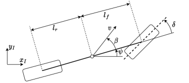
Figure 1: Top view of vehicle single track and single track drift model. The dot in center of the figure represents the center of gravity.

3.1 Reference model

Training and validation data was generated by simulation of the vehicle single track drift model of Common Road’s Python library (Althoff and Würsching, 2020). Its state vector

$$\boldsymbol{x}=[\Delta x,\Delta y,\psi,\delta,v,\beta,\omega,\omega_{\text{f}},\omega_{\text{r}}]^{\top}$$ (7)

consists of the position in x and y ($\Delta x,\Delta y$), the yaw angle $\psi$, the steer angle $\delta$, velocity $v$, slip angle $\beta$, the yaw rate $\omega$, as well as, the front and rear wheel speed $\omega_{\text{f}}$ and $\omega_{\text{r}}$. The exogenous input

$$\boldsymbol{u}=[a_{x},v_{\delta}]^{\top}$$ (8)

is two-dimensional and defined by acceleration $a_{x}$ and steer velocity $v_{\delta}$. The system dynamics are given as

$$\frac{\mathrm{d}\boldsymbol{x}}{\mathrm{d}t}=\begin{bmatrix}v\cos(\psi+\beta)\\ v\sin(\psi+\beta)\\ \omega\\ v_{\delta}\\ \frac{1}{m}[F_{\text{fx}}\cos(\beta-\delta)+F_{\text{fy}}\sin(\beta-\delta)+F_{\text{rx}}\cos(\beta)+F_{\text{ry}}\sin(\beta)]\\ \frac{1}{mv}[F_{\text{fy}}\cos(\beta-\delta)-F_{\text{fx}}\sin(\beta-\delta)-F_{\text{rx}}\sin(\beta)+F_{\text{ry}}\cos(\beta)]-\omega\\ \frac{1}{I_{\text{z}}}\left([F_{\text{fx}}\sin(\delta)+F_{\text{fy}}\cos(\delta)]l_{\text{f}}-F_{\text{ry}}l_{\text{r}}\right)\\ \frac{1}{I_{\text{w}}}(-r_{w}F_{\text{fx}}+t_{\text{b}}T_{\text{b}}+t_{\text{e}}T_{\text{e}})\\ \frac{1}{I_{\text{w}}}(-r_{w}F_{\text{rx}}+(1-t_{\text{b}})T_{\text{b}}+(1-t_{\text{e}})T_{\text{e}})\end{bmatrix}$$

where $r_{\text{w}}$ denotes the effective tire radius, $I_{\text{w}}$ is the wheel inertia and $t_{\text{b}}$, $t_{\text{e}}$ are the split parameters between front and rear axle for the brake and engine torque, respectively. $m$ is the vehicle mass, and $I_{z}$ the moment of inertia about the vertical axis of the vehicle center of gravity. The lateral tire forces $F_{\cdot\text{y}}$ and longitudinal tire forces $F_{\cdot\text{x}}$ are computed using the Pacejka magic formula (Pacjeka, 2012). The indexes r and f stand for rear and front tire, respectively. $T_{\text{e}}$ and $T_{\text{b}}$ are engine and brake torque, respectively. Both are computed from the longitudinal acceleration $a_{x}$.

The model is capable to compute lateral drift and omits conventional small angle approximations for steering and slip angles. Please consult the documentation of the Common Road library (Althoff and Würsching, 2020) for a detailed description of the vehicle single track drift model. The model parameters of the single track drift model are given in Table 1.

Table 1: Model parameters of reference model (single track drift) and ODE model (single track model).

Name	Symbol	Unit	Value
vehicle mass	$m$	kg	1225
distance COG front axle	$l_{f}$	m	0.883
distance COG rear axle	$l_{r}$	m	1.508
friction coefficient	$\mu$	-	1.048
cornering stiffness front and rear	$C_{f}$, $C_{r}$	$\frac{1}{\mathrm{rad}}$	20.89
center of gravity height	$h$	m	0.557
moment of inertia about z axis	$I_{z}$	$10^{3}\mathrm{kgm}^{2}$	1.538
moment of inertia wheels	$I_{w}$	$10^{3}\mathrm{kgm}^{2}$	1.700
split parameter for engine	$t_{e}$	-	1
split parameter for brake	$t_{b}$	-	0.76
effective tire radius	$r_{w}$	m	0.344

3.2 Training and validation data

Three data samples were drawn by simulation of the single track drift reference model in Python and imported in Julia. Each sample consists of 100 seconds simulation data on 0.1 seconds sample rate. Each data sample was split into training and validation set at $t=70\,\mathrm{s}$. The first segment $0<t<70\,\mathrm{s}$ is the training set and the second segment $70\leq t<100\,\mathrm{s}$ is the validation set in each of the tree data samples.

The first two data samples were used for a pre-training, while the last data sample was used for calculation of training and validation error as well as for generating the result plots for each model. The initial state vector at $t=0\,\mathrm{s}$ and exogenous inputs of the third data sample are given in the sequel, whereas the respective data for data sample one and two are omitted for brevity. The initial state vector of the third data sample was $\boldsymbol{x}_{t=0}=[0,0,0,0,25,0,0,0,0]^{\top}$, which means that only the initial vehicle velocity was set to a non-zero value. The exogenous inputs of data sample three became $a_{x}(t)=0.01+0.05\cos(t)+0.1\sin(0.1t)$ and $v_{\delta}(t)=0.02\sin(t)$ respectively. Figure 2 presents both inputs over simulation time.

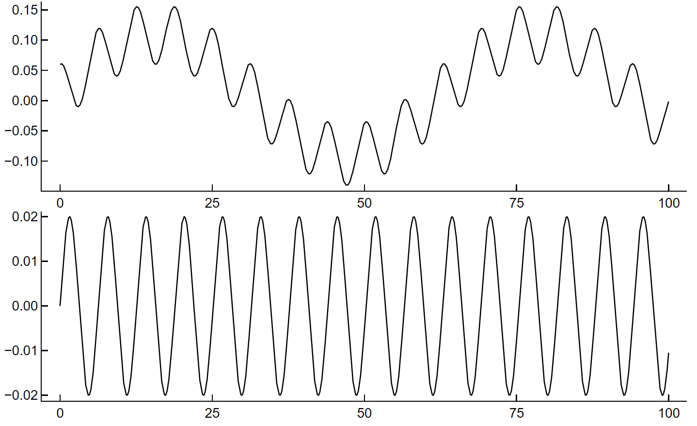
Figure 2: Exogenous input of acceleration ($a_{x}(t)$) and steer angle velocity ($v_{\delta}(t)$) of data sample three in top and bottom panel respectively. The x-axis denotes simulation time in seconds.

Note that $\boldsymbol{x}_{t=0}$, $a_{x}(t)$, and $v_{\delta}(t)$ were slightly modified in data sample one and two to enrich the coverage rate of the state space for training of neural ODE and UDE model.

A z-score data scaler of the states and inputs was fit to the third data sample. This scaler prepares the data for the neural network input layer and for the cost function in the neural ODE and UDE model. In addition, the scaler was used to normalize the reference states for adding white Gaussian noise with zero mean and deviation $\sigma=0.025$ on each reference state. Afterwards, the scaler transformed the noisy reference states back into original space and the noisy reference states show comparable noise level.

3.3 ODE model

The ODE model is inspired by the linear vehicle single track model, see, e.g., Althoff et al. (2017). Its state vector consists of

$$\boldsymbol{x}=[\Delta x,\Delta y,\psi,\delta,v,\beta,\omega]^{\top}$$ (9)

and the dynamics are given as

$$\frac{\mathrm{d}\boldsymbol{x}}{\mathrm{d}t}=\begin{bmatrix}v\cos(\psi+\beta)\\ v\sin(\psi+\beta)\\ \omega\\ v_{\delta}\\ a_{\text{x}}\\ \frac{1}{mv}[F_{\text{fy}}+F_{\text{ry}}]-\omega\\ \frac{1}{I_{\text{z}}}\left(F_{\text{fy}}l_{\text{f}}-F_{\text{ry}}l_{\text{r}}\right)\end{bmatrix}$$ (10)

where the simplified lateral tire forces are

$$F_{\text{fy}}=\mu C_{\text{f}}\frac{mgl_{\text{r}}}{l_{\text{r}}+l_{\text{f}}}\left(\delta-\frac{\dot{\psi}l_{\text{f}}}{v}-\beta\right),F_{\text{ry}}=\mu C_{\text{r}}\frac{mgl_{\text{f}}}{l_{\text{r}}+l_{\text{f}}}\left(\frac{\dot{\psi}l_{\text{r}}}{v}-\beta\right),$$ (11)

where $\mu$ defines the tire road friction coefficient, $C_{f},C_{r}$ are the front and rear cornering stiffness, $h$ is the height of center of gravity above road level, $g$ is the gravitational constant. Additional simplifications compared to the single track drift model are that the wheel slip and thus the wheel speeds as well as the longitudinal forces are neglected. Furthermore, a small angle approximation, i.e. $\cos(x)\approx 1$ and $\sin(x)\approx x$, is carried out. The values of the vehicle parameters were identical in the single track drift and the single track model.

Especially the difference in the tire models cause a systematic model error for the single track model (ODE model), compared with the single track drift model, which generated the training and validation data sets. The single track model serves as ODE benchmark method in the sequel to show the benefit of using data in the following neural ODE and UDE methods.

3.4 Neural ODE model

The neural ODE is given as

$$\frac{\mathrm{d}\boldsymbol{x}}{\mathrm{d}t}=\mathrm{NN}(\mathcal{Z}\{[\boldsymbol{x},\boldsymbol{u}]^{\top}\},\boldsymbol{\theta},t),$$ (12)

where $\mathcal{Z}\{\cdot\}$ means a z-score data transformation. The neural ODE input layer is nine-dimensional and consists of z-score transformed states and exogenous inputs. The hidden layer comprises a varying number of fully connected neurons with $\tanh(\cdot)$ activation function and the output layer models all seven derivatives of the states in (9).

3.5 UDE model

The UDE model is given as

$$\frac{\mathrm{d}\boldsymbol{x}}{\mathrm{d}t}=\begin{bmatrix}v\cos(\psi+\beta)\\ v\sin(\psi+\beta)\\ \omega\\ v_{\delta}\\ \mathrm{NN}(\mathcal{Z}\{[\delta,v,\beta,\omega,a_{x},v_{\delta}]^{\top}\},\boldsymbol{\theta},t)\end{bmatrix},$$ (13)

where the first four relations are identical with the ODE model (10).

Our aim is to remove simple and general physical relations from the learning task of the NN in the UDE model. Hence, the kinematic relations of the four first states are not part of the neural ODE network here. We assume that these relations are in general correct and there is no need to apply machine learning to reveal these certain equations. Accordingly, the neural network within the UDE model is more compact compared with the neural network in the neural ODE model. The neural network in the UDE has six inputs in the input layer and one hidden layer of fully connected neurons with $\tanh(\cdot)$ activation function on varying size. The output layer models the derivatives of the last three states of the state vector in (9). This leads to fewer network weights in the UDE model.

Remark - While the ODE, neural ODE, and UDE model, share the same state vector $\boldsymbol{x}$ and vector of exogenous inputs $\boldsymbol{u}$, the reference model consists of two more states.

3.6 Training

The ODE model does not require parameter estimation or training because it is build from first principles and shares exact vehicle parameters with reference model.

Neural ODE and UDE were deployed on varying size in the hidden layer to find the optimal model complexity in accordance with Occam’s razor. We varied the hidden layer from five up to 12 neurons in neural ODE model and UDE model. Table 2 lists the number of trainable network weights dependent on the hidden layer size for the neural ODE and UDE model. Due to smaller size in input and output layer, the UDE model has in general fewer weights in the network weight matrix $\boldsymbol{\theta}$ compared with the neural ODE network on same hidden layer size.

Table 2: Number of weights in neural network weight matrix $\boldsymbol{\theta}$ over hidden layer size of neural ODE and UDE model.

neurons in hidden layer	5	8	10	12
weights in neural ODE	92	143	177	211
weights in UDE	53	83	103	123

The neural ODE model and UDE model were trained sequentially on the training batches ($0<t<70\,\mathrm{s}$) of data sample one to three. In each training, Julia’s default random number generator initialized the neural network weights to ensure reproducible results and this weight initialization was repeated for five different random number seeds to explore the sensitivity of the optimization result with respect to the initialization. The number of neurons in the hidden layer controls the model complexity. Due to the involved neural network, the neural ODE and UDE model fall under the bias variance dilemma. To few neurons may lead to a model which cannot represent the underlying process, which causes high bias in the model estimates. Too many neurons may cause overfitting and poor prediction capabilities, known as high variance. Hence, we varied the hidden layer size to find the point where the training error and validation error are both acceptable. Following Occam’s razor principle, the best model is the model on good accuracy and parsimony. On the other hand, poor initialization of the neural network weights may cause poor optimization result because the optimizer might get stuck in a local optima. We decided to use random weight initialization for simplicity and spent the effort of five different optimizations for each hidden layer size to reduce the risk of early inferior local optima. This simple but effective setup worked in our experiments. The random initialization of the weights did not result in numerical problems due to initial stiff or unstable neural ODEs. Hence, more advanced initialization methods like collocation pre-training, neutral pre-training, or inclusion of model faders, as discussed in (Thummerer et al., 2022), was not required herein.

In total, we conducted twenty optimizations for neural ODE and UDE model respectively (four different hidden layers times five initialization seeds). ADAM algorithm (Kingma and Ba, 2014) optimized the neural network parameters on 2000 iterations for each data sample. The optimal learning rate for ADAM was found by initial experiments. The hidden layer of neural ODE and UDE were adjusted five to neurons (the smallest net in the sequel) and the learning rate varied within $\alpha=[0.1,0.075,0.05,0.025,0.01,0.001]$.

Standard training on the entire batch of training data failed in the initial experiments, because the optimizer got stuck in local optima, which resulted in constant horizontal state trajectories on high training and validation error. The reason for the poor initial results are the oscillations in the training data. Presenting all data at once with oscillations caused “flattened out” trajectories and was recently reported on other artificially and experimental data in (Turan and Jäschke, 2022). There are two solutions for this problem: incremental learning and multiple shooting. In incremental learning, one splits the training data in smaller segments and presents these segments iteratively to the optimizer. The first training is done on segment one, the next training on segment one and two, and so on. This approach is simple and robust but causes unwanted computational load due to iteratively increasing data size and reuse of training segments. In contrast, multiple shooting is more computational efficient because the cost function is applied to individual data segments and coupled through shooting variables to ensure smooth state transitions at the training segments. Therefore, we applied multiple shooting function of DiffEqFlux.jl (Rackauckas et al., 2019) in all experiments. The segment size was adjusted to 80 data points and the continuity term was set to one.

3.7 Performance criteria

For neural ODE and UDE model, the training and validation error for data sample three was evaluated with the sum of squared errors (SSE)

$$\mathrm{SSE}=\sum\limits_{i=1}^{n}\left(\boldsymbol{x}_{i}-\boldsymbol{\widehat{x}_{i}}\right)^{2},$$ (14)

where $\boldsymbol{x}$ and $\widehat{\boldsymbol{x}}$ are matrices of reference and estimated state trajectories at index $i$. To ensure equal influence of individual state errors, the state trajectories were scaled with z-score transformation before SSE computation. Note that the physical quantities range between $10^{-2}$ and $10^{2}$ in the state space. Hence, certain states would be practically neglected if the cost function would operate on untransformed data.

4 Results and discussion

First, we will present and discuss the benchmark result from ODE model. Then, we will discuss the results of the initial training on varying learning rate for neural ODE and UDE model and present the results of neural ODE and UDE model with variation in hidden layer size and network weight initialization. Finally, the best neural ODE and UDE model state trajectories are presented.

4.1 ODE model

Figure 3 compares the simulated state trajectories of the ODE single track model with the reference states from the single track drift model. All states in Figure 3 (and Figures 5, 6, 7) are given in SI units over time in $\mathrm{s}$. The positions $x$ and $y$ in $\mathrm{m}$, yaw angle $\psi$ and steer angle $\delta$ in $\mathrm{rad}$, velocity $v$ in $\mathrm{m}\text{\,}{\mathrm{s}}^{-1}$, slip angle $\beta$ in $\mathrm{rad}$, and yaw rate $\omega$ in $\mathrm{rad}\text{\,}{\mathrm{s}}^{-1}$.

Although all model parameters like vehicle mass, cornering stiffness are identical in ODE in reference model, the ODE model shows poor accuracy. The positions in panel one and two, yaw angle $\psi$ in panel three, velocity $v$ in panel five drift away from reference data in time. The ODE model overestimates the oscillation in the slip angle $\beta$ in panel six and in the yaw rate $\omega$ in the last panel. To sum up, the neglected drift effect in the simple ODE model causes a large model error in comparison with the reference data from the single track drift model. Due to its poor accuracy, we will exclude the ODE model in the following in detail result presentation.

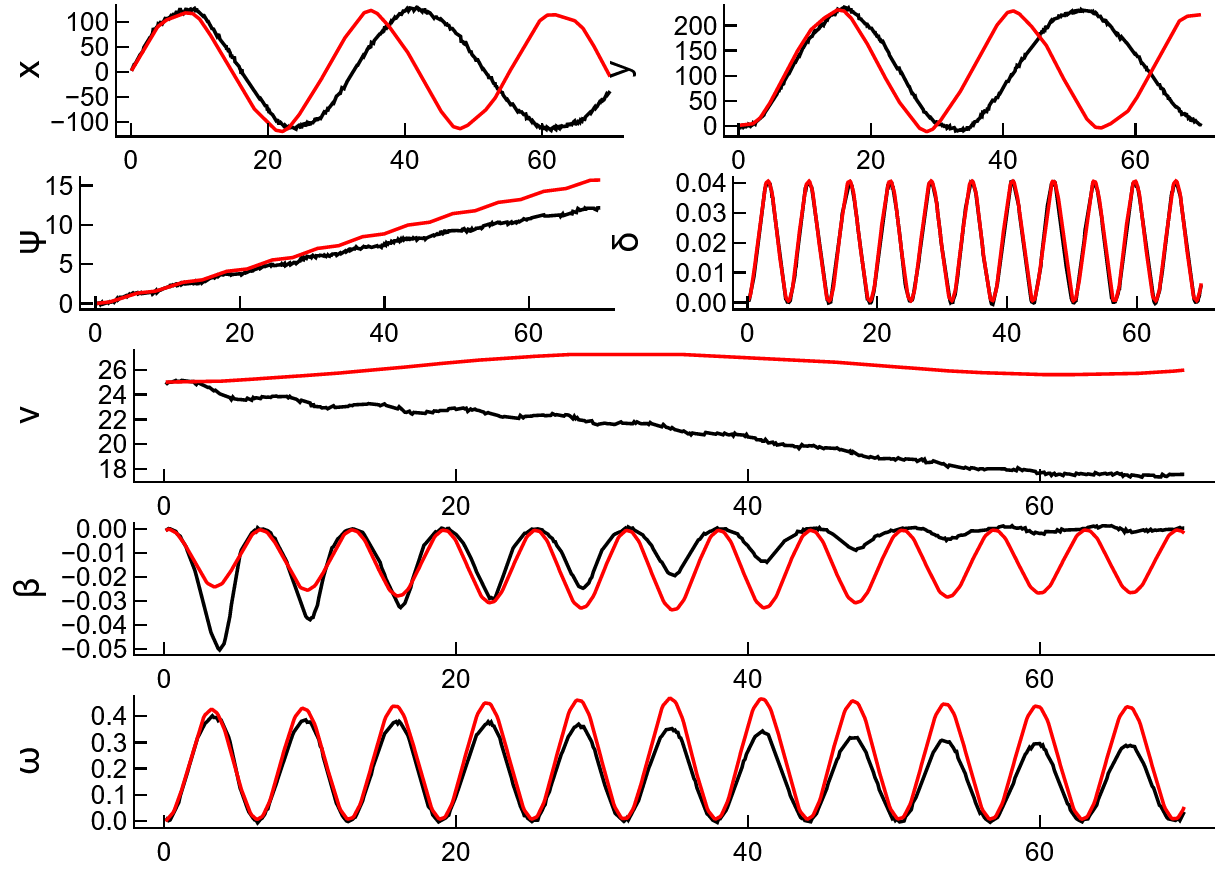
Figure 3: Estimated state trajectories of ODE model (red line) and reference model (black line) over the training batch. Note the large deviation between ODE mode and reference data in the velocity $v$ (fifth panel).

4.2 Varying the learning rate for neural ODE and UDE model

Table 3 lists the training and validation error of neural ODE and UDE model for each learning rate. The smallest training error of neural ODE was found by a learning rate of 0.05, whereas the UDE model gave the smallest training error at $\alpha=0.025$. Overall, the UDE training and validation errors are less sensitive to variation in learning rate than the neural ODE errors. Specifically, the smallest and largest learning rates cause poor accuracy in the neural ODE model, where the UDE model still produces acceptable results. Finally, we selected $\alpha=0.05$ for ADAM optimization of neural ODE weights and $\alpha=0.025$ for UDE weights.

Table 3: Training and validation error over learning rate for neural ODE (nODE) and UDE model, each with hidden layer of five neurons. The errors were computed on z-score transformed data with sum of squared errors. The smallest training errors are written in bold. The sum of squared error of the ODE model for simulation scenario used in the training is 7988, yielding a performance improvement of $7988/125\approx 63\%$ and $7988/117\approx 68\%$ for the nODE and UDE model, respectively.

	training error		validation error
learning rate	nODE	UDE	nODE	UDE
0.1	2327	122	1301	50
0.075	230	249	539	225
0.05	125	134	972	125
0.025	143	117	810	47
0.01	104202	145	895	103
0.001	128670	163	10434	31

4.3 Varying hidden layer and initialization in neural ODE and UDE model

Table 4 shows the training and validation error over increasing number of neurons in the hidden layer, and on varying random initialization for the neural ODE and UDE model. In contrast to the learning rate selection, we focus here on small validation error to find the best hidden layer size and initialization for neural ODE and UDE model. Accordingly, the best neural ODE and UDE result was found with ten neurons in the hidden layer. However, the best initialization for neural ODE was the fifth, whereas best UDE model was optimized on first initialization. Therefore, the in depth results of neural ODE and UDE model will be presented with 10 in the hidden layer and the respective random number setting in the next sections. Strikingly, the optimization is highly sensitive to the initialization of network. Some initialization cause large validation error. For instance the UDE model with twelve neurons and random number seed two appears as outlier. Therefore, either repetitive initializations on different seeds (as done herein), or more advanced initializations methods must be applied in neural ODE experiments in order to compare different model structures.

Again, the neural ODE model shows often larger variation in errors than the UDE model and in the error level of neural ODE model is roughly one order of magnitude larger than the validation error of the UDE model. However, both models show some outliers in the validation when the initialization caused a remarkably poor fit. In neural ODE, a steady decrease of training error over growing number of neurons in the hidden layer is visible, which is supported by machine learning theory. The evolution of training error in UDE model is rather stable, which does not result in concrete conclusions.

Table 4: Training and validation error of neural ODE (nODE) and UDE model over varying hidden layer size. Rng colum denotes experiments where the random number seed of network weights initialization was varied. The smallest validation errors are written in bold.

		training error		validation error
hidden layer size	rng	nODE	UDE	nODE	UDE
5	1	125	117	972	47
	2	216	126	863	120
	3	350	82	3667	156
	4	1926	148	1185	53
	5	247	118	1209	24
8	1	49	127	821	59
	2	27	115	681	39
	3	59	189	1045	156
	4	20	182	679	124
	5	29	133	851	22
10	1	20	119	1343	16
	2	16	116	942	41
	3	15	152	816	133
	4	72	143	1159	413
	5	13	206	349	343
12	1	20	173	614	67
	2	25	199	547	4686
	3	19	163	623	260
	4	22	140	759	98
	5	16	125	440	117

Figure 4 presents the same data as Table 4 in another format. Here, the validation errors for each neural ODE and UDE model is drawn over the number of neural network weights, which represents the model complexity. Models on same structure but different initializations are connected with solid vertical lines. Apart from one outlier on twelve neurons, all UDE model build a cluster in the lower left edge of the figure, which means that almost all UDE models show higher accuracy than the neural ODE models. Moreover, we found initializations where the smallest UDE models on five and eight neurons were roughly as accurate as the best UDE model with ten neurons. Hence, one could also argue to prefer a smaller UDE model in practical applications than the model that we have selected. Add to this, the complexity of many UDE models is smaller than the neural ODE models. Hence, the UDE models are in general the better choice following Occam’s razor. With focus on accuracy, neural ODE and UDE with 10 neurons in hidden layer are best in each model class.

Figure 4: Validation error of all neural ODE (nODE) and UDE model over the number of neural network weights. The subscripts in the model names denote the hidden layer size. For instance, UDE₁₀ means the UDE model with ten neurons in the hidden layer. Dots connected with vertical lines denote repeated trainings on different initialization of the network weights. Please note the logarithmic scale of the validation error.

4.4 Neural ODE₁₀ model

Figure 5 gives the estimated states over simulation time for the neural ODE model with 10 neurons in the hidden layer on rng seed five. The model shows high accuracy for the training batch ($t<70\,\mathrm{s}$), but the states diverge from reference data in the validation set from $t>70\,\mathrm{s}$ onwards. This accuracy drop in the validation is mainly driven by the position states in first and second panel, yaw angle in third panel, and velocity in fifth panel. The other states show slight error in validation. Compared with the benchmark ODE model in Figure 3, the neural ODE model is more accurate. The numerical values for training and validation error of the neural ODE₁₀ model can be found in Table 4.

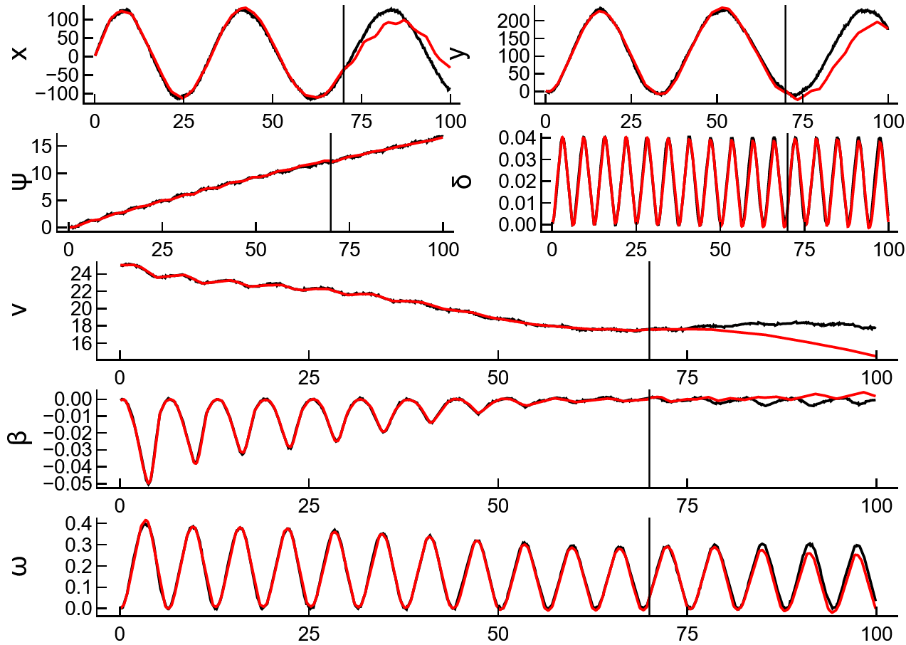
Figure 5: Estimated state trajectories of neural ODE₁₀ model with 10 neurons in hidden layer (red line) and reference model (black line). The vertical line at $t=70\,\mathrm{s}$ marks the split between training and validation data.

4.5 UDE₁₀ model

Figure 6 gives the estimated states over simulation time for the UDE model with 10 neurons in the hidden layer on rng seed one. UDE₁₀ is not as accurate as neural ODE₁₀ in training batch, but superior accurate in the validation set among all models. Considering the relative small number neural network weights of UDE₁₀ (103 weights), this model is the best model in the set of candidate models. The smaller accuracy in training but higher accuracy invalidation indicates that the model generalized the data better than neural ODE₁₀ model. However, the first two position states of UDE₁₀ start to diverge from reference roughly in the middle of the training batch at $t>30\,\mathrm{s}$. On the other hand, the introduced physical relations for the yaw angle $\mathrm{d}\psi/\mathrm{d}t=\omega$ and steer angle $\mathrm{d}\delta/\mathrm{d}t=v_{\delta}$ in (13) appear to improve the accuracy compared with neural ODE₁₀ model.

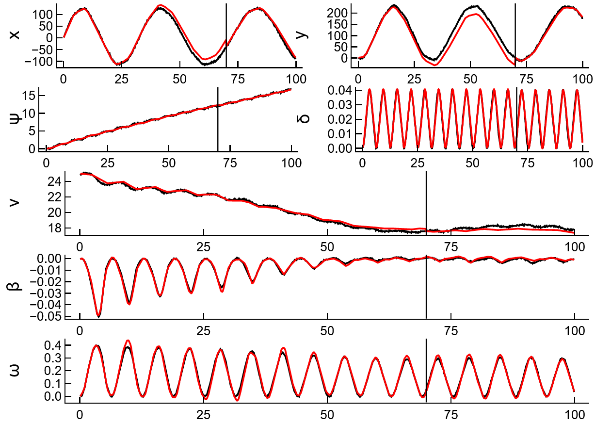
Figure 6: Estimated state trajectories of UDE₁₀ model with 10 neurons in hidden layer (red line) and reference model (black line). Training and validation set is split at $t=70\,\mathrm{s}$, indicated by the black vertical line.

4.6 UDE₅ model

Finally, Figure 7 gives the estimated states over simulation time for the UDE model with 5 neurons in the hidden layer on rng seed five. This model is nearly as accurate as the previous UDE₁₀ model, but more efficient in required storage for network weights, in training, and in evaluation time. Therefore, the compact UDE₅ might be preferable in embedded functions where storage and processing power are very limited. However, the UDE₅ model does not capture all dynamics in the velocity between $20<t<50$ seconds compared with UDE₁₀ and reference data. Instead, the velocity trajectory is rather flat and smooth.

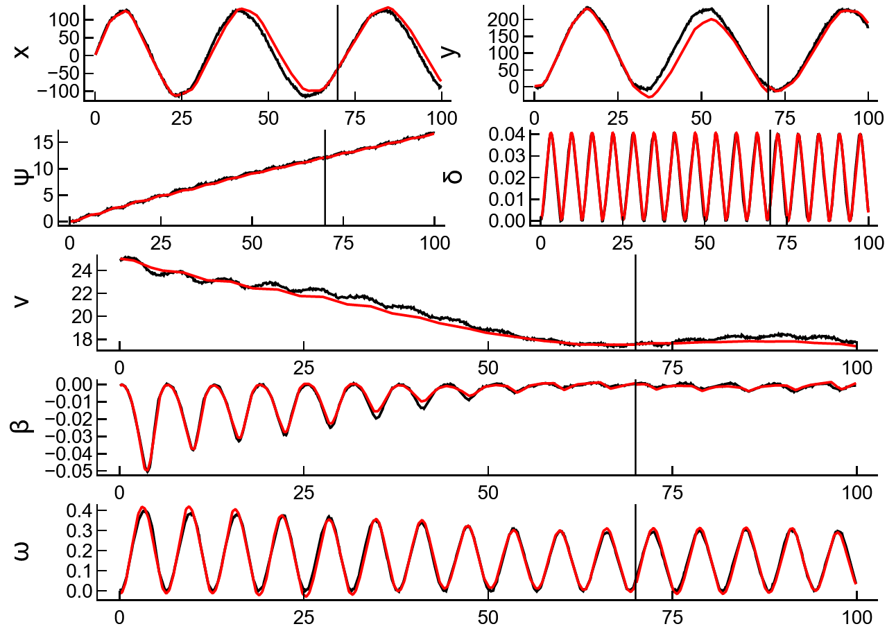
Figure 7: Estimated state trajectories of UDE₅ model with 5 neurons in hidden layer (red line) and reference model (black line). Training and validation set is split at $t=70\,\mathrm{s}$, indicated by the black vertical line.

5 Conclusions

This comparative study of different modeling methods, ranging from physics based modeling with a vehicle single track ODE model, over black box modeling with neural differential equations (NODE), to hybrid modeling through universal differential equations (UDE), showed that the UDE approach was superior in terms of validation accuracy and model complexity. In specific, the UDE₁₀ model corrected missing physical effects of a conventional vehicle single track ODE model through the neural ODE part in the states of vehicle velocity, slip angle and yaw rate. Add to this, the hybrid model took favor of physics based kinematic state equations for vehicle positions, yaw angle, and steer angle in order to improve the prediction accuracy for these states compared with the pure black box neural ODE model.

Moreover, the combination of physics based differential equations and neural differential equations allowed to reduce the size of the neural network significantly compared with a pure black box model, which helps to reduce training and evaluation time and limits required storage for network weights in embedded applications. In conclusion, the UDE₁₀ combines to a certain extent the predictability, generalization and interpretability of physical modeling with adaptation to training data of machine learning and was superior accurate than each modeling approach individually.

In the future, more investigation is needed to study how the hybrid model performs in other scenarios. We are looking also for methods to add uncertainty estimates to the modeled states to receive a confidence measure. This is especially important for states modeled by a neural network and allows for a credibility assessment of the model. Another field of research is to detect and prevent the evaluation of the data-based part far beyond the dynamics captured by the seen learning data. In this case one would rely on extrapolation capabilities, which a data-based model does not have in general. These measures are required for accreditation of hybrid models in real world applications such as advanced driver assistance systems.

Declaration of interests

This work was supported by the ITEA3-Project UPSIM (Unleash Potentials in Simulation) № 19006, see: https://www.upsim-project.eu/ for more information. Add to this, all authors report financial support, provided by Robert Bosch GmbH and Stephan Rhode has patent pending to German Patent and Trademark Office.

CRediT authorship contribution statement

Stephan Rhode: Conceptualization, Methodology, Software, Validation, Investigation, Writing - Original Draft, Writing - Review & Editing, Visualization. Fabian Jarmolowitz: Writing - Original Draft. Felix Berkel: Writing - Original Draft.

References

- Althoff et al. (2017) Althoff, M., Koschi, M., Manzinger, S., 2017. Commonroad: Composable benchmarks for motion planning on roads, in: 2017 IEEE Intelligent Vehicles Symposium (IV), pp. 719–726. doi:10.1109/IVS.2017.7995802.
- Althoff and Würsching (2020) Althoff, M., Würsching, G., 2020. Common road python library. URL: https://pypi.org/project/commonroad-vehicle-models/. version 2.0.0.
- Bonfitto et al. (2020) Bonfitto, A., Feraco, S., Tonoli, A., Amati, N., 2020. Combined regression and classification artificial neural networks for sideslip angle estimation and road condition identification. Vehicle System Dynamics 58, 1766–1787. doi:10.1080/00423114.2019.1645860.
- Chen et al. (2018) Chen, R.T.Q., Rubanova, Y., Bettencourt, J., Duvenaud, D., 2018. Neural ordinary differential equations. doi:10.48550/arXiv.1806.07366.
- Devineau et al. (2018) Devineau, G., Polack, P., Altché, F., Moutarde, F., 2018. Coupled longitudinal and lateral control of a vehicle using deep learning, in: 2018 21st International Conference on Intelligent Transportation Systems (ITSC), pp. 642–649. doi:10.1109/ITSC.2018.8570020.
- Essa et al. (2021) Essa, M.G., Elias, C.M., Shehata, O.M., 2021. Comprehensive performance assessment of various nn-based side-slip angle estimators (ann-sse), in: 2021 IEEE 93rd Vehicular Technology Conference (VTC2021-Spring), pp. 1–6. doi:10.1109/VTC2021-Spring51267.2021.9448647.
- Gräber et al. (2019) Gräber, T., Lupberger, S., Unterreiner, M., Schramm, D., 2019. A hybrid approach to side-slip angle estimation with recurrent neural networks and kinematic vehicle models. IEEE Transactions on Intelligent Vehicles 4, 39–47. doi:10.1109/TIV.2018.2886687.
- Guo et al. (2018) Guo, H., Cao, D., Chen, H., Lv, C., Wang, H., Yang, S., 2018. Vehicle dynamic state estimation: state of the art schemes and perspectives. IEEE/CAA Journal of Automatica Sinica 5, 418–431. doi:10.1109/JAS.2017.7510811.
- Hermansdorfer et al. (2020) Hermansdorfer, L., Trauth, R., Betz, J., Lienkamp, M., 2020. End-to-end neural network for vehicle dynamics modeling, in: 2020 6th IEEE Congress on Information Science and Technology (CiSt), pp. 407–412. doi:10.1109/CiSt49399.2021.9357196.
- James et al. (2020) James, S.S., Anderson, S.R., Lio, M.D., 2020. Longitudinal vehicle dynamics: A comparison of physical and data-driven models under large-scale real-world driving conditions. IEEE Access 8, 73714–73729. doi:10.1109/ACCESS.2020.2988592.
- Karpatne et al. (2017) Karpatne, A., Atluri, G., Faghmous, J.H., Steinbach, M., Banerjee, A., Ganguly, A., Shekhar, S., Samatova, N., Kumar, V., 2017. Theory-guided data science: A new paradigm for scientific discovery from data. IEEE Transactions on Knowledge and Data Engineering 29, 2318–2331. doi:10.1109/TKDE.2017.2720168.
- Katriniok et al. (2013) Katriniok, A., Maschuw, J.P., Christen, F., Eckstein, L., Abel, D., 2013. Optimal vehicle dynamics control for combined longitudinal and lateral autonomous vehicle guidance, in: 2013 European Control Conference (ECC), pp. 974–979. doi:10.23919/ECC.2013.6669331.
- Kingma and Ba (2014) Kingma, D.P., Ba, J., 2014. Adam: A method for stochastic optimization. doi:10.48550/arXiv.1412.6980.
- Liniger et al. (2014) Liniger, A., Domahidi, A., Morari, M., 2014. Optimization-based autonomous racing of 1:43 scale RC cars. Optimal Control Applications and Methods 36, 628–647. doi:10.1002/oca.2123.
- Ljung (1999) Ljung, L., 1999. System identification: theory for the user. Prentice Hall information and system sciences series. 2nd ed ed., Prentice Hall PTR, Upper Saddle River, NJ.
- Ma et al. (2021) Ma, Y., Dixit, V., Innes, M.J., Guo, X., Rackauckas, C., 2021. A comparison of automatic differentiation and continuous sensitivity analysis for derivatives of differential equation solutions, in: 2021 IEEE High Performance Extreme Computing Conference (HPEC), pp. 1–9. doi:10.1109/HPEC49654.2021.9622796.
- Mazor et al. (1998) Mazor, E., Averbuch, A., Bar-Shalom, Y., Dayan, J., 1998. Interacting multiple model methods in target tracking: a survey. IEEE Transactions on Aerospace and Electronic Systems 34, 103–123. doi:10.1109/7.640267.
- Melzi and Sabbioni (2011) Melzi, S., Sabbioni, E., 2011. On the vehicle sideslip angle estimation through neural networks: Numerical and experimental results. Mechanical Systems and Signal Processing 25, 2005–2019. doi:10.1016/j.ymssp.2010.10.015. interdisciplinary Aspects of Vehicle Dynamics.
- Pacjeka (2012) Pacjeka, H., 2012. Tyre and Vehicle Dynamics. third ed., Elsevier. doi:10.1016/C2010-0-68548-8.
- Pontryagin et al. (1962) Pontryagin, L.S., Boltyanskii, V.G., Gamkrelidze, R.V., Mishchenko, E.F., 1962. The mathematical theory of optimal processes. Authorized translation from the Russian. Translator: K. N. Trirogoff. Editor: L. W. Neustadt. New York and London: Interscience Publishers, a division of John Wiley & Sons, Inc., viii, 360 p. (1962).
- Rackauckas et al. (2019) Rackauckas, C., Innes, M., Ma, Y., Bettencourt, J., White, L., Dixit, V., 2019. Diffeqflux.jl - a julia library for neural differential equations doi:10.48550/arXiv.1902.02376.
- Rackauckas et al. (2020) Rackauckas, C., Ma, Y., Martensen, J., Warner, C., Zubov, K., Supekar, R., Skinner, D., Ramadhan, A., Edelman, A., 2020. Universal differential equations for scientific machine learning doi:10.48550/arXiv.2001.04385.
- Rahman et al. (2022) Rahman, A., Drgoňa, J., Tuor, A., Strube, J., 2022. Neural ordinary differential equations for nonlinear system identification, in: 2022 American Control Conference (ACC), pp. 3979–3984. doi:10.23919/ACC53348.2022.9867586.
- Rai and Sahu (2020) Rai, R., Sahu, C.K., 2020. Driven by data or derived through physics? a review of hybrid physics guided machine learning techniques with cyber-physical system (cps) focus. IEEE Access 8, 71050–71073. doi:10.1109/ACCESS.2020.2987324.
- Raissi et al. (2019) Raissi, M., Perdikaris, P., Karniadakis, G., 2019. Physics-informed neural networks: A deep learning framework for solving forward and inverse problems involving nonlinear partial differential equations. Journal of Computational Physics 378, 686–707. doi:10.1016/j.jcp.2018.10.045.
- Rhode (2022) Rhode, S., 2022. Github repository with companion code. URL: www.github.com/stephanrhode/hybrid_node.
- Roehrl et al. (2020) Roehrl, M.A., Runkler, T.A., Brandtstetter, V., Tokic, M., Obermayer, S., 2020. Modeling system dynamics with physics-informed neural networks based on lagrangian mechanics. IFAC-PapersOnLine 53, 9195–9200. doi:10.1016/j.ifacol.2020.12.2182. 21st IFAC World Congress.
- von Rueden et al. (2021) von Rueden, L., Mayer, S., Beckh, K., Georgiev, B., Giesselbach, S., Heese, R., Kirsch, B., Walczak, M., Pfrommer, J., Pick, A., Ramamurthy, R., Garcke, J., Bauckhage, C., Schuecker, J., 2021. Informed machine learning - a taxonomy and survey of integrating prior knowledge into learning systems. IEEE Transactions on Knowledge and Data Engineering , 1–1doi:10.1109/TKDE.2021.3079836.
- Schoukens and Ljung (2019) Schoukens, J., Ljung, L., 2019. Nonlinear system identification: A user-oriented road map. IEEE Control Systems Magazine 39, 28–99. doi:10.1109/MCS.2019.2938121.
- Schramm et al. (2018) Schramm, D., Hiller, M., Bardini, R., 2018. Vehicle Dynamics. Springer. doi:10.1007/978-3-662-54483-9.
- Sieberg et al. (2022) Sieberg, P.M., Blume, S., Reicherts, S., Maas, N., Schramm, D., 2022. Hybrid state estimation–a contribution towards reliability enhancement of artificial neural network estimators. IEEE Transactions on Intelligent Transportation Systems 23, 6337–6346. doi:10.1109/TITS.2021.3055800.
- Singh et al. (2019) Singh, K.B., Arat, M.A., Taheri, S., 2019. Literature review and fundamental approaches for vehicle and tire state estimation. Vehicle System Dynamics 57, 1643–1665. doi:10.1080/00423114.2018.1544373.
- Söderström and Stoica (1989) Söderström, T., Stoica, P., 1989. System Identification. Prentice-Hall Software Series, Prentice Hall.
- Spielberg et al. (2019) Spielberg, N.A., Brown, M., Kapania, N.R., Kegelman, J.C., Gerdes, J.C., 2019. Neural network vehicle models for high-performance automated driving. Science Robotics 4. doi:10.1126/scirobotics.aaw1975.
- Thummerer et al. (2022) Thummerer, T., Stoljar, J., Mikelsons, L., 2022. Neuralfmu: Presenting a workflow for integrating hybrid neuralodes into real-world applications. Electronics 11. doi:10.3390/electronics11193202.
- Turan and Jäschke (2022) Turan, E.M., Jäschke, J., 2022. Multiple shooting for training neural differential equations on time series. IEEE Control Systems Letters 6, 1897–1902. doi:10.1109/LCSYS.2021.3135835.
- Viana et al. (2021) Viana, F.A., Nascimento, R.G., Dourado, A., Yucesan, Y.A., 2021. Estimating model inadequacy in ordinary differential equations with physics-informed neural networks. Computers & Structures 245, 106–458. doi:10.1016/j.compstruc.2020.106458.
- Wenzel et al. (2006) Wenzel, T., Burnham, K.J., Blundell, M.V., Williams, R.A., 2006. Dual extended Kalman filter for vehicle state and parameter estimation. Vehicle System Dynamics 44, 153–171. doi:10.1080/00423110500385949.
- Willard et al. (2022) Willard, J., Jia, X., Xu, S., Steinbach, M., Kumar, V., 2022. Integrating scientific knowledge with machine learning for engineering and environmental systems. ACM Comput. Surv. doi:10.1145/3514228.
- Yi et al. (2016) Yi, B., Gottschling, S., Ferdinand, J., Simm, N., Bonarens, F., Stiller, C., 2016. Real time integrated vehicle dynamics control and trajectory planning with mpc for critical maneuvers, in: 2016 IEEE Intelligent Vehicles Symposium (IV), pp. 584–589. doi:10.1109/IVS.2016.7535446.
- Yim and Oh (2004) Yim, Y.U., Oh, S.Y., 2004. Modeling of vehicle dynamics from real vehicle measurements using a neural network with two-stage hybrid learning for accurate long-term prediction. IEEE Transactions on Vehicular Technology 53, 1076–1084. doi:10.1109/TVT.2004.830145.