The role of Ohmic dissipation of internal currents on Hot Jupiter radii

Abstract

Aims. The inflated radii observed in hundreds of Hot Jupiters represent a long-standing open issue. The observed correlation between radii and irradiation strength, and the occasional extreme cases, nearly double the size of Jupiter, remain without a comprehensive quantitative explanation. In this investigation, we delve into this issue within the framework of Ohmic dissipation, one of the most promising mechanisms for explaining the radius anomaly.

Methods. Using the evolutionary code MESA, we simulate the evolution of irradiated giant planets, spanning the range 1 to 8 Jupiter masses, incorporating an internal source of Ohmic dissipation located beneath the radiative-convective boundary. Our modeling is based on physical parameters, and accounts for the approximated conductivity and the evolution of the magnetic fields, utilizing widely-used scaling laws. We compute the radius evolution across a spectrum of masses and equilibrium temperatures, considering varying amounts of Ohmic dissipation, calculated with the internal conductivity profile and an effective parametrization of the currents, based on the typical radius of curvature of the field lines.

Results. Our analysis reveals that this internal Ohmic dissipation can broadly reproduce the range of observed radii using values of radius of curvature up to about one order of magnitude lower than what we estimate from the Juno measurements of the Jovian magnetosphere and from MHD dynamo simulations presented herein. The observed trend with equilibrium temperature can be explained if the highly-irradiated planets have more intense and more small-scale magnetic fields. This suggests the possibility of an interplay between atmospherically induced currents and the interior, via turbulence, in agreement with recent box simulations of turbulent MHD in atmospheric columns.

1 Introduction

The intriguing exoplanet class of “Hot Jupiters” (HJs) currently consists of several hundred objects, discovered and characterized in terms of mass and radius. These gas giant planets are tidally locked, with orbital periods of a few days, corresponding to distances within $\sim 0.1$ AU of their host stars (for a review, see Heng & Showman 2015 and Fortney et al. 2021). The proximity to the host star implies strong irradiation of their day sides, which results in typical equilibrium temperatures of up to $3000$ K, with a few even hotter. The intense irradiation flux, coupled with the strong thermal gradients due to the tidal locking, gives rise to powerful atmospheric flows, with equatorial super-rotation and strong day-night flows which try to redistribute the heat across the planetary surface (Cho et al., 2008; Dobbs-Dixon & Lin, 2008; Showman et al., 2009; Heng et al., 2011; Rauscher & Menou, 2012; Perna et al., 2012; Rauscher & Menou, 2013; Perez-Becker & Showman, 2013; Parmentier et al., 2013; Rogers & Showman, 2014; Showman et al., 2015; Kataria et al., 2015; Koll & Komacek, 2018; Beltz et al., 2022; Komacek et al., 2022; Dietrich et al., 2022).

Observations of HJs reveal that a substantial fraction of them have radii that are significantly larger than those predicted by standard cooling evolutionary models (e.g. Showman & Guillot 2002 and Wang et al. 2015), even when accounting for the effect of the irradiation itself alone, able to inflate the radius up to only $\sim 20\%$ more (Guillot et al., 1996; Arras & Bildsten, 2006; Fortney et al., 2007). Several explanations have been proposed, which can be broadly classified into two categories: (1) The first one invokes planetary evolution with a delayed cooling, such as in the case of a large atmospheric opacity (Burrows et al., 2007). As the opacity increases, cooling becomes inefficient and planets can retain more internal heat. (2) The second category relies on the presence of additional heat sources in the interior of the planet. Various mechanisms have been proposed for such thermal dissipation: hydrodynamic dissipation (involving the conversion of the stellar flux into the kinetic energy of the global atmospheric flow due to the large day-night temperature gradient, e.g. Showman & Guillot 2002 and Showman et al. 2009), dissipation of heat via tidal forces (Bodenheimer et al., 2001), inhibition of large-scale convection (Chabrier & Baraffe, 2007), dissipation of energy induced by fluid instabilities (Li & Goodman 2010), forced turbulence in the radiative layer (Youdin & Mitchell 2010), and Ohmic dissipation (Batygin & Stevenson, 2010; Perna et al., 2010b).

Among these proposed mechanisms, the last one, Ohmic dissipation, has received considerable attention in the last few years (Batygin et al., 2011; Huang & Cumming, 2012; Wu & Lithwick, 2013; Rauscher & Menou, 2013; Rogers & Showman, 2014; Rogers & Komacek, 2014; Ginzburg & Sari, 2016; Rogers & McElwaine, 2017; Hardy et al., 2022; Beltz et al., 2022; Benavides et al., 2022; Knierim et al., 2022). Magnetohydrodynamic (MHD) coupling between the deep-seated magnetic field and the atmospheric flow of thermally ionized particles (mostly free electrons from alkali metals) leads to currents which dissipate at deeper levels, resulting in an additional heat source for the planet, and hence a larger radius for the same mass and age. While the extent of the magnetic drag (Perna et al., 2010a) in reducing flow speeds (and hence, the magnitude of Ohmic dissipation) is still debated, this heating source appears consistent with observations (Laughlin et al., 2011). There is also the possibility that more than one mechanism may operate simultaneously (Sarkis et al., 2021).

Although much less often considered in previous works, Ohmic dissipation can also occur in deeper convective regions, which connect the atmosphere to the interior of the planet, where the magnetic field is continuously regenerated by the convection and rotation of the high-pressure metallic hydrogen (e.g. Zaghoo & Silvera 2017 and Zaghoo & Collins 2018). Whether such a dynamo mechanism, active in Jupiter and Saturn, is operative in HJs as well, which have a much slower rotation, is yet to be established. Inferring parameters about Ohmic dissipation can then also shed light into this.

The goal of this paper is to study the long-term evolution (on Gyr timescales) of HJs, especially examining how the internal Ohmic heating component modifies the characteristic properties of the planets and, in particular, the evolution of their radii. Using a specifically modified version of the public code MESA (Paxton et al., 2019), we run a grid of simulations for a range of planetary masses and equilibrium temperatures, and show how such models can explain the observed distribution of the inflated radii of HJs. Our study is similar in spirit to those of e.g. Komacek & Youdin (2017), Komacek et al. (2020) and Thorngren & Fortney (2018) in their exploration of the effects of the deposition of (unspecified) heat sources at different depths on the planetary long-term evolution. The novelty here regards the physical parameters that define the sources of heat. In particular, we: (i) use conductivity profiles inspired by existing models, throughout all the interior; (ii) evaluate the depth-dependent Ohmic power by means of a few effective parameters to compute the current intensity, with reference values that lean on Jupiter data and a set of MHD dynamo simulations; and (iii) evolve the magnetic field intensity via scaling laws, adapted for HJs.

The paper is organized as follows: §2 describes the observational data available from the NASA Exoplanet Archive. §3 describes the standard evolutionary models for HJs as implemented in MESA, and §4 presents our Ohmic heating model and its major ingredients. §5 shows a sample of different results of the simulations. Finally, our conclusions and discussion are presented in §6.

2 Observational sample of Hot Jupiters

Here we present a short overview of the relevant recent observational data on HJs obtained from the NASA Exoplanet Archive. Although as of mid-February 2024 there were a total of 1775 confirmed gas giants with known masses between $0.5$ and $13M_{\rm J}$, only 417 of those have available information about their mass, radius, age and equilibrium temperature, which are the quantities we are interested in.

Since the radius is our main observable to compare with, we have excluded data with high errors in radius, and only selected those planets with errors less than $25\%$. This yields a data set of 397 Jupiter-like planets, shown in Fig. 1. Planet radii are plotted versus the equilibrium temperature of the planet defined by,

$$T_{\rm eq}=\left(\frac{R_{\star}}{2d}\right)^{1/2}T_{\star}\,,$$ (1)

where $R_{\star}$ and $T_{\star}$ are the observed radius and effective temperature of the host star, and $d$ is the star-planet separation. As usual, this definition ignores the unknown planetary albedo and the atmospheric greenhouse effects, and assumes a complete heat redistribution over the entire planetary surface.

It can be observed from Fig. 1 that the radii of the planets increase as the equilibrium temperature rises. However, this effect is noticeable only for planets with $T_{\rm eq}\sim 1000$ K or higher. Since our focus is on studying Ohmic dissipation as an inflation mechanism, here we concentrate on planets with this temperature or above.

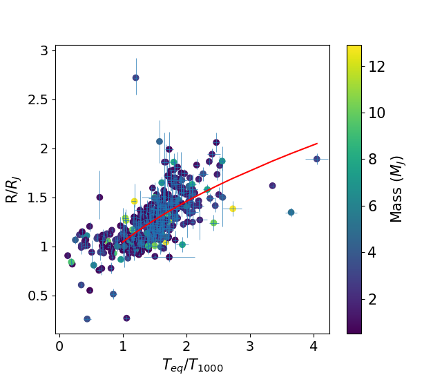
Figure 1: Planetary radius (in units of Jupiter radius, $R_{\rm J}$) versus equilibrium temperature (in units of $1000$ K) for the 397 Jupiter-like exoplanets in the database with available mass, age, radius and equilibrium temperature data, and which have errors in radius of less than 25%. The mass is shown on a color scale. The red line (only shown for temperatures above 1000 K) indicates the best fit power-law model to the data and corresponds to $\log(R/R_{\rm J})=\log(1.044\pm 0.020)+(0.481\pm 0.035)\log(T_{\rm eq}/T_{1000})$.

3 Theoretical overview of the evolutionary model

We model the evolution of HJs using the publicly available code MESA (Paxton et al., 2011, 2013, 2019). The equations solved by MESA are the one dimensional time-dependent equations of stellar structure applied to gas giants. The first is the conservation of mass,

$$\frac{dm}{dr}=4\pi r^{2}\varrho\,,$$ (2)

where $m$ is the mass enclosed within the radius $r$, and $\varrho$ is the density. Next, we have the equation of hydrostatic equilibrium,

$$\frac{dP}{dm}=-\frac{Gm}{4\pi r^{4}}\,,$$ (3)

where $P$ is the pressure and $G$, the gravitational constant. The energy conservation is given in terms of the luminosity $L$,

$$\frac{dL}{dm}=\epsilon_{\rm grav}+\epsilon_{\rm irr}+\epsilon_{\rm dep}\,,$$ (4)

where $\epsilon_{\rm grav}=-TdS/dt$ is the heating term due to gravitational contraction or inflation, with $S$ being the specific entropy and $T$ the temperature; $\epsilon_{\rm irr}$ is heating due to irradiation, while $\epsilon_{\rm dep}$ represents any additional heat deposition (in our case, Ohmic dissipation in the interior). Lastly, the energy transport equation is given by,

$$\frac{dT}{dm}=-\frac{GmT}{4\pi r^{4}P}\nabla\,,$$ (5)

where $\nabla=d\ln T/d\ln P$ is the logarithmic temperature gradient (set to the smallest between the adiabatic gradient and the radiative gradient).

These equations are closed using the MESA equation of state (Paxton et al., 2019), which basically consists of the interpolation of the SCvH (Saumon–Chabrier–van Horn) equation of state (Saumon et al., 1995) for the temperatures and densities relevant for gas giants.

3.1 Composition and Structure

In all our models, we employ a uniform Solar composition, i.e. with He mass fraction and metallicity fixed to $Y=0.24$ and $Z=0.02$, respectively. Additionally, we allow for the presence of an inert core, which in this study we fix to $M_{\rm core}=10M_{\oplus}$ ($M_{\oplus}$ being the mass of the Earth) with a constant density of 10 g cm^-3. This is certainly a simplification of a more complex, multi-layer structure, favored by the Jovian models fitting Galileo and Juno gravity data (Debras & Chabrier, 2019). In these models, the core consists of a few tens of Earth masses (and similarly for Saturn). For the purposes of this study, we do not explore different models of the core. We have confirmed that varying the core mass alone affects the planetary radius by an additional few percents, as previously reported by Fortney et al. (2007). See the recent dedicated work by Yıldız et al. (2024) for a MESA study of the Solar System giants’ interiors.

3.2 Irradiation and atmospheric modeling

MESA provides a few different ways to implement an irradiated atmosphere. As in Komacek & Youdin (2017), we use the simplest one: an energy generation rate of $\epsilon_{\rm irr}=F_{\star}/4\Sigma_{\star}$ applied uniformly in the outer mass column $\Sigma\leqslant\Sigma_{\star}$. Here $F_{\star}=\sigma T_{\rm eq}^{4}$ is the day-side flux from the host star. As in Komacek & Youdin (2017), we fix $\Sigma_{\star}=250$ g cm^-2 for the mass column, corresponding to an opacity of $\kappa=4\times 10^{-3}$ g^-1 cm². This value, for a non-irradiated $1M_{\rm J}$ planet at 5 Gyr, would correspond to a pressure of approximately 1 bar.

Note also that, since the model is 1D, we cannot model the effects of irradiation being effective only on the day side. Hence, the local values of the temperature in the outer layer must be interpreted as averages.

3.3 Standard cooling models

As a reference and comparison with well-known results from the literature, we briefly show illustrative examples for the planetary structure with no extra heating (by setting $\epsilon_{\rm dep}=0$ in equation 4). In Fig. 2, we show the $P(T)$ profiles for a planet of mass $1M_{\rm J}$ with an equilibrium temperature of 1500 K, at three different ages. In the same plot, we indicate the position of the convective regions (marked by thick lines) and the radiative regions (marked with thin lines). As the internal heat decreases over time, the $P(T)$ lines move downwards, and the radiative–convective boundary (RCB) gets deeper, reaching typical pressures of kbar at Gyr. This is in agreement with what has been widely discussed in previous works, for example in Arras & Bildsten (2006), Fortney et al. (2007), Komacek & Youdin (2017) and Thorngren et al. (2019).

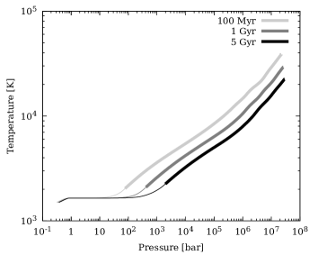
Figure 2: Temperature as a function of pressure at various moments throughout the evolution of a planet of $1M_{\rm J}$ with an equilibrium temperature of $T_{\rm eq}=1500$ K and no Ohmic heating. The thicker lines correspond to the convective zone (extending all the way to the center). The age for each line is indicated in the key, where it goes from youngest for the top line to the oldest for the bottom line.

In Fig. 3, we show the radius evolution for planets of two different masses at three different irradiation levels (equilibrium temperatures). As expected, we find positive trends between inflation and mass or irradiation, but the radius can increase up to at most $\sim 20\%$, in agreement with the early results by e.g. Guillot et al. (1996) and Fortney et al. (2007). The consistency of our results with the existing literature validates the baseline models, on top of which we add the Ohmic heating model, as described next.

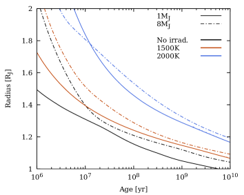
Figure 3: Evolution of the radii of planets with masses $1M_{\rm J}$ (solid lines) and $8M_{\rm J}$ (dash-dotted lines), up to an age of 10 Gyr when no Ohmic heating is present. Three sets of curves are shown: black lines are for no irradiation; red lines are for $T_{\rm eq}=1500$ K; and blue lines are for $T_{\rm eq}=2000$ K. Here we show the cases for relatively high temperatures, as the inflation for $T_{\rm eq}<1000$ K remains relatively moderate (close to the black lines). Note that the maximum inflation for the models shown here is approximately 20%.

4 Ohmic heating model

In this section we describe our extension of the MESA code, to include the extra heating term due to Ohmic dissipation, whose volumetric rate is estimated by,

$$Q=\frac{J^{2}}{\sigma}\,,$$ (6)

where $J$ is the electrical current and $\sigma$ the electrical conductivity. This heating term is added as an additional source in the energy equation (equation 4) evolved by MESA,

$$\epsilon_{\rm dep}=\frac{Q}{\varrho}\,.$$ (7)

Below we detail how we parameterize $Q$. Our approach is to assume values of the internal conductivity profile similar to those adopted in the literature, and consider the minimal number of free parameters for the estimation of the currents. Such an effective approach allows us to build a simple but quantitative model which is able to span a broad range of relevant physical parameters, which can then be constrained by a HJ population comparison.

4.1 Location of the dynamo region

Ohmic dissipation is possible both in the metallic hydrogen region, where the deep-seated dynamo is supposed to operate, and in the shallower layers, where the atmospheric winding in the radiative layers (Batygin & Stevenson, 2010; Perna et al., 2010b; Dietrich et al., 2022) and possibly the turbulence (Soriano-Guerrero et al., 2023, 2024) can amplify and twist the deep-seated magnetic field. Ideally, we would need prescriptions for the currents and for the electrical conductivity in both regions, and understand how they interact. This is so far quantitatively unexplored and our aim is to have a minimal, but physically-based Ohmic model.

Since we want to keep to a minimum the number of effective parameters, by default we fix the location of the deposition of heat. We consider as a fiducial case one where Ohmic dissipation occurs below 800 bar, a value well within the convective region when Ohmic heating is included (see below). Furthermore, we consider a variant in which the dissipation region starts immediately below the RCB, which evolves and depends on the planetary properties (Fortney et al., 2007; Thorngren et al., 2019).

4.2 Conductivity

In the deep regions of gas giants (for pressures in the range of $\sim 0.2-5$ kbar), hydrogen transitions to a metallic state with a high electrical conductivity. This transformation occurs through the breaking of hydrogen molecules into individual atoms accompanied by the release of electrons, which can move freely (Lorenzen et al., 2011). Various models have been proposed, including notably those of French et al. (2012) and Zaghoo & Collins (2018) (and references therein). These models differ by almost one order of magnitude in the values of $\sigma(P)$, but they predict the transition to happen around $5\times 10^{5}-10^{6}$ bar.

At shallower layers, including the atmosphere, the conductivity is dominated by thermal ionization. Previous efforts (Batygin & Stevenson, 2010; Perna et al., 2010b) have mostly focused on the conductivity of the atmospheric layers ($P\lesssim 100$ bar), since that is where the winds can directly induce currents via winding. These works are usually based on simplifications (Batygin & Stevenson, 2010) or on classical recipes (Draine et al. 1983 and references within, see their § III) that approximate (within a certain range of validity) the contribution from the partially ionized potassium (Balbus & Hawley, 2000), which is the first alkaline metal to get ionized for local temperatures $T\lesssim 2200$ K (Dietrich et al., 2022). Recent calculations by Kumar et al. (2021) have obtained the conductivity up to $10^{4}$ K for densities $\leq 10^{-2}$ g cm^-3, fully accounting for the partial ionization of all species. Although the general trends with temperature and density are compatible with the classical approximations, there are non-negligible differences for a given profile $T(P)$, especially with the rough approximation by Batygin & Stevenson (2010) (see Fig. 10 of Kumar et al. 2021). Besides these model uncertainties, the conductivity depends on the composition, which can vary on a case by case basis, and in the cited papers this has been kept fixed.

Generally, for the convective, non-metallic hydrogen region ($\lesssim 10^{6}$ bar), we expect the thermal partial ionization of alkaline components to be dominant and be able to conduct currents. In this work, contrarily to previous studies which focused only into the outermost layers ($P\lesssim 100-1000$ bar), we take such deep layers into account, since the magnetic field generated in the atmosphere by winding can become turbulent, as seen in our local box simulations which consider small-scale perturbations (Soriano-Guerrero et al., 2023), and can propagate downwards (Soriano-Guerrero et al., 2024). The idea of the downward propagation of turbulent motions was put forward by Youdin & Mitchell (2010) as a mechanical greenhouse effect, and, under the presence of conductivity, this will create small magnetic structures as well.

Given the high uncertainties mentioned above, we adopt a unique conductivity profile for all cases, which strongly increases in the metallic hydrogen region. While this profile is arbitrary, the uncertain deviations from the real profile are encapsulated in our only free Ohmic parameter, $\ell$, as we show below. The conductivity profile we adopt is shown in Fig. 4 (solid black line), together with the profiles of the metallic hydrogen from French et al. (2012) and Zaghoo & Collins (2018), and with the potassium contribution calculated as in Perna et al. (2010b) and references within. The latter is shown for the profiles of irradiated planets at 5 Gyr, for three different values of $T_{\rm eq}$. Our conductivity is a bit higher than the models in the literature, a choice that we take in order to be conservative, as for a given $J$, low values of $\sigma$ would produce more Ohmic heating (equation 6). Also note that the precise value of the conductivity at large depths is irrelevant, since it is very high — the global dissipation is dominated by the least conductive regions.

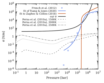
Figure 4: Conductivity profile used in this work (solid black line). As a reference we indicate those for metallic hydrogen from French et al. (2012) (together with the fit by Tsang & Jones 2020) and from Zaghoo & Collins (2018), as well as those from the partial thermal ionization of alkaline metals. For the latter, we consider three different cases of irradiated planets without Ohmic heating (with $T_{\rm eq}=1500$, 2000 and 2500 K), taking their $T$, $P$ and $\rho$ profiles at 5 Gyr from our MESA simulations. With these values, we calculate the conductivity using the approximation for the contribution from ionized potassium as in Perna et al. (2010b) and references within, assuming a potassium abundance of $10^{-7}$ and a molecular weight $\mu=2$. Note that we extend such formulae down to very high pressures just for comparison purposes: the validity of the formulae is likely restricted to shallower layers.

4.3 Magnetic field estimate

The estimation of the currents is much less constrained, since the planetary magnetism is known only for the Solar System (surface magnetic fields $B\lesssim 10$ G), where it shows a great case-by-case variety. No reliable measurements of exoplanet magnetic fields are available. Some model-dependent interpretations of Ca II emissions observed in a few HJs indicate up to $\sim 100$ G surface fields (Cauley et al., 2019). In fact, HJs are considered as the most promising targets for the first exoplanetary radio detection at low frequencies, powered by the interaction of the stellar wind with their magnetic fields, or by star-planet magnetic interaction (see Grießmeier et al. 2007; Zarka 2007). So far, only a tentative, inconclusive claim of exoplanetary radio detection has been raised (Turner et al., 2021), which is not surprising due to the intrinsically low frequencies and flux expected — a conclusive measurement of exoplanetary magnetic fields is still missing.

Given the lack of observational constraints, and in order to keep the model as simple as possible in terms of the number of parameters, we estimate the magnetic field intensity from the scaling law given in Reiners et al. (2009) and Reiners & Christensen (2010), which expresses the field strength at the surface of the dynamo in terms of other planetary properties,

$$B=4.8\times 10^{3}\left(\frac{ML^{2}}{R^{7}}\right)^{1/6}\,{\rm G}.$$ (8)

In this formula, the planetary mass $M$, luminosity $L$ and radius $R$ are expressed in solar units. This scaling law is in agreement with what is observed in the Solar system. Indeed, Christensen et al. (2009) showed that in a broad range of masses (from rocky planets to main-sequence stars), the measured magnetic field scales well with the internal heat flux, even though surprisingly high values of radio-inferred brown dwarf magnetic fields have later challenged this relation (Kao et al., 2016, 2018).

In our model, the luminosity $L$ is the surface one, which is set by $T_{\rm eq}$. This means that we are extending the relation given through equation (8), so far applied to stars and cold planets, also to hot giants. This can be considered as an indirect incorporation of the amplification of the field (due to the winding in the shallow layers and the turbulence possibly propagating inwards) in addition to the deep-seated dynamo field. Therefore, the value of the magnetic field here has to be interpreted as an average one over the regions with the relevant Ohmic dissipation. If provided by turbulent amplification, it is possibly much higher than the dipolar field which can extend to the magnetosphere. We will discuss the implications of this assumption and the results in terms of atmospheric dynamics and the interplay with the deep-seated field.

With these assumptions, we expect the magnetic field estimated via equation (8) to scale as $B\sim T_{\rm eq}^{4/3}R^{-1/2}$, where the radius $R$ itself also depends to a certain degree on the irradiation and heat deposition. Since $R$ evolves, we take into account how $B$ also changes with time. Just as a phenomenological reference, if we assume the best-fit power law slope similar to the one shown in Fig. 1, i.e. $R\sim T_{\rm eq}^{1/2}$, then one expects an almost linear relation, $B\sim T_{\rm eq}^{15/12}$.

4.4 Estimation of the currents

For our purposes, the relevant quantity is the amount of currents in the conductive regions. We can parameterize Ampère’s law, which is given in Gaussian units as,

$$\boldsymbol{J}=\frac{c}{4\pi}\boldsymbol{\nabla}\times\boldsymbol{B}\,,$$ (9)

by considering the magnetic field strength $B$ from equation (8) and defining a typical length scale $\ell=B/|\boldsymbol{\nabla}\times\boldsymbol{B}|$, which measures how the magnetic field changes, to obtain,

$$J=\frac{cB}{4\pi\ell}\,.$$ (10)

The length scale $\ell$ is representative of the radius of curvature of the magnetic field lines. In order to obtain a reasonable estimate of its value, we have taken a two-fold approach that we describe below in 4.4.1 (based on Juno observations of Jupiter) and 4.4.2 (based on numerical MHD simulations). Once we adopt an electrical conductivity profile and a prescription for the magnetic field strength, the only free, undetermined parameter in our model is the length scale $\ell$, which can then be varied to find the range that best matches the bulk of HJ radii. For simplicity, we will keep this length scale constant with respect to the planetary radius throughout the evolution (i.e. we fix $\ell$ to be a certain fraction of $R$), while the magnetic field intensity evolves. We motivate this choice further in 4.4.2.

We expect small values of $\ell$ for the currents and conductivity just below the RCB, primarily associated with atmospheric induction, which may propagate downwards through turbulence (Soriano-Guerrero et al., 2023, 2024). Instead, we use an estimate for $\ell$ in the dynamo region ($P\gtrsim 10^{6}$ bar) derived from Jupiter data and simulations.

The Joule heating rate is now given through (using equations 6 and 10),

$$Q=\frac{J^{2}}{\sigma}=\left(\frac{c}{4\pi}\right)^{2}\frac{B^{2}}{\ell^{2}\sigma}\,.$$ (11)

Note that the combination $\ell^{2}\sigma$ is what determines $Q$. By fixing the value of $\sigma$, we are combining all uncertainties in the values of the conductivity and radius of curvature into the single parameter $\ell$.

Finally, note that, in previous works, the simple relation $J\propto\sigma B$ was used (Batygin & Stevenson, 2010). However, in the non-linear regime, such as the turbulent one expected in HJs with $T_{\rm eq}\gtrsim 1500$ K (Dietrich et al., 2022; Soriano-Guerrero et al., 2023), this relation is no longer valid, since the magnetic induction from the wind does not simply produce a perturbation on the existing, internally-generated fields. Instead, magnetic fields can become much more intense, and in this non-linear regime it is not clear which recipe to use for the currents, unless a proper MHD simulation for each specific case is performed. The same applies for the outer part of the dynamo region (where the hydrogen conductivity declines) — dynamo simulations (Gastine & Wicht, 2021; Yadav & Thorngren, 2017) (and our own simulations, see below) show how the currents drop in the regions where the conductivity drops.

4.4.1 Evaluation of a typical length scale from Juno observations

We have considered the Juno measurements of the Jovian magnetic field above the surface, which is represented in terms of multipolar decomposition of the poloidal and toroidal components, as given by the best-fit model to the data (Connerney et al., 2018, 2022). With the set of these best-fitting weights, one can describe the magnetic field in the entire volume where there are no currents, down to the internal radius below which the dynamo starts to be active. From that, one can calculate the average radius of curvature of the field lines, where the curvature (i.e. the inverse of the radius of curvature) is defined by,

$$\boldsymbol{\kappa}=(\boldsymbol{b}\cdot\boldsymbol{\nabla})\boldsymbol{b}\,,$$ (12)

where $\boldsymbol{b}\equiv\boldsymbol{B}/B$. We consider the radial profile, taking spatial averages over a sphere at a given radius, $\bar{\kappa}$. In Appendix A, we show that, for Jupiter, the inferred value of the radius of curvature, averaged over a spherical surface, is typically $1/\bar{\kappa}\sim 0.07-0.3R_{\rm J}$, depending on the magnetospheric model used and the depth considered. We adopt this estimate of the curvature of the magnetic field as a lower possible value, i.e. a maximum typical magnetic length scale $\ell$ defined as $1/\bar{\kappa}$. The reason is that we expect the curvature to increase in the inner dynamo region of the planet as a consequence of the turbulent environment in which the magnetic field is amplified.

4.4.2 Radial behaviour from MHD simulations

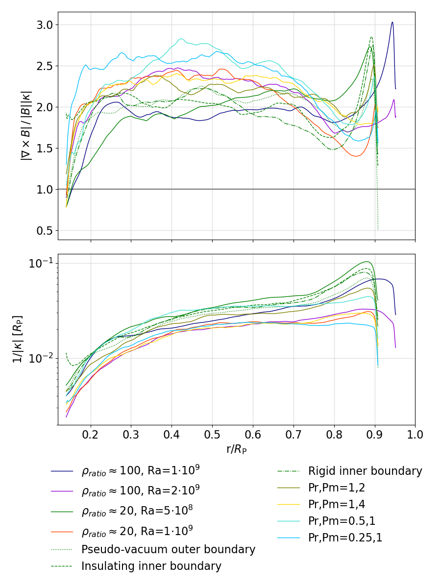
Figure 5: Typical radial profiles of $|\boldsymbol{\nabla}\times\boldsymbol{B}|/(\bar{\kappa}B)$ (top) and $1/\bar{\kappa}$ (bottom), averaged over the spherical surface at each radius, from 3D dynamo simulations with the code MagIC. In order to explore the sensitivity to the free parameters. All models have the same boundary conditions (i.e. stress-free for the fluid and insulating for the magnetic fields outside, stress-free and perfectly conducting inside) except for the cases marked in the legend. The Ekman number is $10^{-5}$, and both Prandtl numbers are set to 1 (except for those also marked in the legend, which have $\rho_{\rm ratio}\approx 20$ and ${\rm Ra}=5\times 10^{8}$. Note that $\ell=1/\bar{\kappa}$ becomes much smaller close to the external boundary, in order to match with the potential configuration constraint. See Appendix B for more details.

While we can infer the minimum value of $\boldsymbol{\kappa}$, and hence the maximum value of $\ell$, from Juno measurements, we need to understand how $\ell$ behaves in the dynamo region. To do so we performed MHD dynamo simulations that allowed to estimate the values of the currents, and to validate the use of $\bar{\kappa}$ as a proxy for $\ell$. We have used the code MagIC (Jones et al., 2011; Gastine & Wicht, 2012) to study the amplification of the magnetic field in HJ-like planets. We used a variety of dynamo parameters and boundary conditions, and a representative structure profile for conductivity, density and other thermodynamic quantities, coming from our irradiated HJ MESA models. We defer the more relevant details to Appendix B and will describe the main results of this study in an upcoming dedicated paper. These simulations provide us a self-consistent evolution of the magnetic field as amplified in the convective, turbulent interior of a HJ, and, therefore, allow a robust estimation of the typical length scale $\ell$.

We show the results in Fig. 5, where only some representative models producing a dynamo are shown. Despite some small differences among the various simulations, we obtain radial profiles with the same trend and order of magnitude, both for $|\boldsymbol{\nabla}\times\boldsymbol{B}|/(\bar{\kappa}B)=1/(\bar{\kappa}\ell)\sim 1-3$ and $1/\bar{\kappa}\sim(0.01-0.1)R_{\rm J}$. For the former (top panel), it confirms that the ratio between the magnetic field intensity and the mean radius of curvature, $B\bar{\kappa}$, is a very good tracer of the currents $J$. Regarding $\bar{\kappa}$ itself (bottom panel), we obtain values similar to the ones inferred from Juno data (Appendix A), showing what might be the typical expected values for $\ell$.

It is important to notice that we cannot easily extract the value of planetary magnetic fields from MHD simulations, since we cannot easily reach numerical convergence and therefore the magnetic field strength depends on the resolution. Moreover, the dynamo parameters used, such as the Rayleigh, Ekman and Prandtl numbers, are not realistic in this kind of MHD simulations due to computational constraints. However, we tested that the radial behaviour of $\ell$ does not change with resolution, hence, we can safely work with the hypothesis of a constant $\ell$. With these elements in hand, we can therefore estimate the role of the Ohmic heating due to currents, through the parameter $\ell$.

5 Results: Radius evolution as a function of the model parameters

In this section, we present results from MESA simulations for the evolution of planets over 10 Gyr, under the presence of Ohmic heating, focusing mostly on the planetary radius $R_{\rm P}$. We study how the results depend on the three main parameters of our model: the planetary mass, the equilibrium temperature, and the magnetic length scale $\ell$. We vary the former two within ranges that cover most of the observed values ($1-8M_{\rm J}$ and $1000-2000$ K), while for the latter we consider values around the one inferred from Jupiter data, $\ell\sim 10^{-2}R_{\rm P}$ (as discussed in §4.4), and smaller values, to test more extreme cases. All other model parameters are kept fixed, either because their variations within realistic ranges are known to have smaller effects compared to the observed radii (as is the case for the core mass, the composition and the atmospheric model) (Fortney et al., 2007), or because their intrinsic uncertainties can be ultimately reabsorbed into the effective magnetic length scale parameter $\ell$ (such as the conductivity profile, the depth of the dynamo region, and the magnetic field scaling law).

We start with Fig. 6, which shows the magnetic field strength at the dynamo surface for a planet of mass $1M_{\rm J}$ for various equilibrium temperatures (without irradiation, at 1500 K and at 2000 K). While for cold Jupiters, we recover typical Jovian values ($\sim 10$ G at 5 Gyr), irradiated planets show magnetic field amplitudes of hundreds of G, with values going up to $\sim 1$ kG in the most extreme case shown here (for $T_{\rm eq}=2000$ K). The scaling law (equation 8) implies indeed stronger magnetic fields for planets of higher luminosity. The addition of Ohmic heating (dashed and dotted lines for $\ell=10^{-2}R_{\rm P}$ and $10^{-3}R_{\rm P}$, respectively) implies a slightly lower and more steady value of the inferred field at Gyr compared to the non-irradiated cases (for which instead it slightly increases). These trends are a direct consequence of the radius inflation and the scaling law assumed in our model, as discussed above.

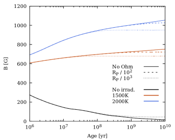
Figure 6: Evolution of the magnetic field strength (estimated from equation 8) for a planet of mass $M_{\rm J}$, with and without Ohmic heating, for the cases of no irradiation (black lines), $T_{\rm eq}=1500$ K (red lines) and $T_{\rm eq}=2000$ K (blue lines). Cases without Ohmic heating are shown with solid lines and those with Ohmic heating are shown with dashed lines (for $\ell=R_{\rm P}/10^{2}$) and dotted lines (for $\ell=R_{\rm P}/10^{3}$).

In order to understand the interior structure of an irradiated, Ohmically heated planet, in Fig. 7, we plot the radial profiles of pressure for a $1M_{\rm J}$ planet at 5 Gyr, for the same three temperatures as above, with and without Ohmic dissipation and for $\ell=10^{-3}R_{\rm P}$. Compared to the non-irradiated case (for which we recover the Jovian radius, solid black line), both irradiation and Ohmic dissipation are able to inflate the outermost part ($\lesssim$ few bars) of the planet. Overall, with this dissipation rate, Ohmic heating results in larger radial extents at similar pressure levels. As a consequence, the interior pressure is also smaller.

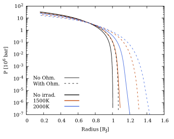
Figure 7: Pressure profile for a planet of mass $M_{\rm J}$ at the age of 5 Gyr for three different irradiation levels (no irradiation in black, 1500 K in red, and 2000 K in blue). The case without Ohmic heating is shown in solid lines and the case with Ohmic heating is shown in dashed lines. The curvature parameter for the Ohmic heating is $\ell=R_{\rm P}/10^{3}$. The lines start at $\sim 0.2R_{\rm J}$, which is the size occupied by the inert core.

Next, we focus on the radius evolution. The left panel of Fig. 8 shows the evolution for three values of $\ell$ and for three values of $T_{\rm eq}$ for a planet of mass $1M_{\rm J}$. We note the strong dependence of the evolution on the value of both parameters. In the figure we also show the case for the extreme value $\ell=R_{\rm P}/10^{4}$. While this value is certainly smaller than typical radii of curvature inferred from Jupiter data or MHD simulations, note that our $\ell$ implicitly incorporates the uncertainties in the values of both the radius of curvature and conductivity as noted in §4.4. Also note that, while we keep the value of $\ell$ fixed throughout the evolution, it most likely would be evolving as well, as the magnetic field structure changes over time. The maximum inflated radii at Gyr ages, for $T_{\rm eq}=2000$ K, go up from $\sim 45\%$ for $\ell=R_{\rm P}/10^{3}$ to $\sim 75\%$ for $\ell=R_{\rm P}/10^{4}$. Decreasing $\ell$ further increases the Ohmic heating beyond the point where the planetary evolution can be followed with MESA. This might be either due to numerical issues close to the boundary, or due to the physical evaporation of the loosely-bound outermost planetary layers. In any case, we do not focus on such cases here, and only show stable simulations.

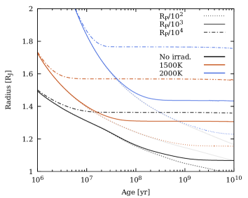
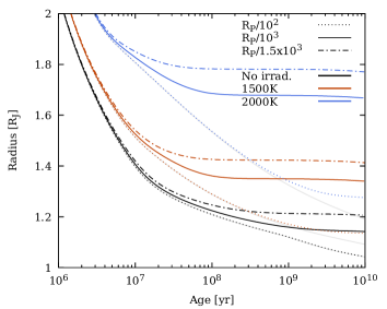
Figure 8: Evolution of the radius $R_{\rm P}$ for a planet of mass $1M_{\rm J}$ (left panel) and $8M_{\rm J}$ (right panel), for various values of the curvature parameter $\ell$ (shown with different line styles, as indicated in the upper legends). We show the cases for non-irradiated planet (black lines), $T_{\rm eq}=1500$ K (red lines), and $T_{\rm eq}=2000$ K (blue lines). The case of irradiation only (without Ohmic heating, Fig. 3) is shown in grey lines in the background for the sake of comparison.

An important feature to note is the fact that, with all the parameters being the same, radius inflation is more intense for larger values of the equilibrium temperature. This is a consequence of the dependence of the magnetic field, and thus Ohmic dissipation, on $T_{\rm eq}$, as discussed in Sec. 4.3.

In the right panel of Fig. 8 we show the evolution of a planet with a larger mass, $8M_{\rm J}$. Since the scaling law for the magnetic field strength implies a stronger field for larger masses, the feasible values of $\ell$ cannot be as large as for smaller-mass planets. Comparing the radius evolution for the same value of $\ell$ in the two panels of Fig. 8, we can indeed see that the larger-mass planet possesses a larger radius for the same $\ell$ and $T_{\rm eq}$. The maximum inflation shown (for $T_{\rm eq}=2000$ K) is close to 70% for $\ell=R_{\rm P}/10^{3}$. Moreover, note that for a cold Jupiter (corresponding to the black lines on the left panel) the case of $\ell=R_{\rm P}/100$ (shown in dotted black lines), which is the expected approximate value of $\ell$, does not provide any inflation compared to the case without Ohmic heating (shown as the grey line in the background). This validates the range of values for our parameters and sets a reference value for $\ell$.

In Fig. 9, we show how the RCB pressure evolves over time for a planet of mass $M_{\rm J}$. As noted in the past (Komacek & Youdin, 2017; Thorngren et al., 2019), increasing the temperature pushes the RCB inwards to larger pressures, while increasing the Ohmic heating pushes the RCB outwards to lower pressures, $\lesssim 100$ bar. This implies that our fiducial value for the dynamo surface lies within the convective region.

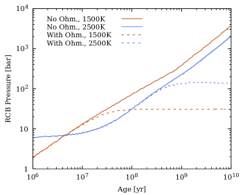
Figure 9: Evolution of the RCB pressure for a planet of mass $M_{\rm J}$ with and without Ohmic heating at $T_{\rm eq}=1500$ K (red lines), and at $T_{\rm eq}=2500$ K (blue lines). The curvature parameter is $\ell=R_{\rm P}/10^{3}$. Here, we show the innermost pressure where the central convective region ends. Particularly at low $T_{\rm eq}$, multiple convective regions can form in the interior near the surface. Moreover, the planet may switch between single and multiple convective regions throughout its evolution. In the cases shown here, there is only one convective region.

In order to compare to the results shown until here, we have run simulations with the Ohmically heated region extending all the way out to the RCB, which itself varies over time. The simulations tend to be more unstable for this variable range case, particularly for high values of $T_{\rm eq}$ or Ohmic heating, in comparison to the fixed range case. A sample of such simulations is shown in Fig. 10. We note that inflation is slightly higher for the variable range (by about 5 to 10%). Hence, leaving the outer pressure boundary fixed can be considered as a conservative limit for the amount of radius inflation due to the internal Ohmic heating.

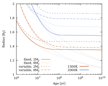
Figure 10: Evolution of the radii of planets of mass $2M_{\rm J}$ and $8M_{\rm J}$ up to an age of 10 Gyr, in the presence of Ohmic heating. The case of extending the Ohmic heating all the way up to the RCB is labeled “variable”, while the usual case we adopt of fixing the pressure range for the heating is labeled “fixed”. Cases for two equilibrium temperatures are shown: 1500 K in red lines and 2000 K in blue lines. The curvature parameter for all cases shown here is $\ell=R_{\rm P}/10^{3}$. The corresponding lines for the cases without Ohmic heating are shown as gray lines in the background as a reference. Allowing the Ohmic dissipation region to vary (thus extending it to larger volumes) increases its effect further, and allows reaching up to 80% radius inflation for the more extreme cases shown here, compared to the maximum of 20% due to irradiation alone (see Fig. 3) and the maximum of 70% for the case of a fixed pressure range (for the same value of $\ell$, Fig. 8).

In Fig. 11, we show the ratio of Ohmic heating to irradiation. For the cases shown here, this “efficiency” reaches only a few percent, in line with previous findings, especially from Bayesian inference (Thorngren & Fortney, 2018). However, this is not strictly required to be the case. At low temperatures and for larger planets, where Ohmic heating is stronger, this ratio naturally will be larger than 1.

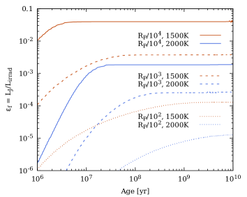
Figure 11: Evolution of the fraction of Ohmic heating to irradiation ($\varepsilon_{\rm f}$) for a planet of mass $M_{\rm J}$ at two different temperatures (1500 K in red and 2000 K in blue) and for three different curvature parameters ($\ell=R_{\rm P}/10^{4}$ in solid lines, $\ell=R_{\rm P}/10^{3}$ in dashed lines, and $\ell=R_{\rm P}/10^{2}$ in dotted lines).

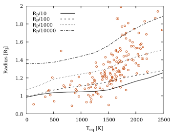
Figure 12: Asymptotic planetary radius (at late ages) versus equilibrium temperature for models with Ohmic heating (for various values of $\ell$) for a $1\leavevmode\nobreak\ M_{\rm J}$ planet. The case for $\ell=R_{\rm P}/10$ is practically the same as the no Ohmic case. The HJ data for planets of mass $0.8<M_{\rm P}/M_{\rm J}<2$ is shown as red circles. For visualization purposes, three outliers (within the same range of masses) below $0.8R_{\rm J}$ and one above $2R_{\rm J}$ are not shown, but they can be identified in Fig. 1.

A broad comparison between the results of our evolutionary models and the data can be seen in Fig. 12. Here, the asymptotic planetary radius (typically reached at an age of 10 Gyr, but that can be reached much earlier depending on the case) of a Jupiter-mass planet is plotted as a function of the equilibrium temperature for various amounts of Ohmic heating, as controlled through the parameter $\ell$. Data for HJs with masses in the range $0.8<M_{\rm P}/M_{\rm J}<2$ is superimposed to the model predictions. The visual comparison shows that, for the models to be able to broadly reproduce the entire range of the data, the parameter $\ell$ needs to be $\gtrsim 100$ times smaller than what is expected from the deep-seated dynamo (or for a cold Jupiter) for a sizable fraction of the population, and in particular, for the planets at higher $T_{\rm eq}$. In other words, the larger the equilibrium temperature, the smaller the value of $\ell$ needed to match the data. In our model, this may indicate a combination of two factors: (i) an overestimation of the assumed conductivity with respect to the real one (see Fig. 4); or (ii) a smaller length scale of the magnetic fields. In the second case, this might indicate that, in a wide range of pressures, large values of very small-scale magnetic fields are maintained. This is compatible with turbulent fields, generated in the shallow layer, penetrating at greater depths despite the relatively low (but not negligible) conductivity. Since the uncertainties of our models are summarized substantially by the parameter $\ell$, and the quantity determining the inflation is the total amount of heat deposited below the RCB, regardless of its spatial distribution, we cannot constrain separately the magnetic properties (its intensity and radius of curvature) and the conductivity profiles.

6 Summary and Conclusions

In this work, via a suite of numerical simulations with the code MESA, we have investigated the evolution of Jupiter-like planets, subject to both a varying degree of irradiation, as well as a varying amount of internal heating. While similar in spirit to the work of Komacek & Youdin (2017), here the internal source of heating is assumed to be of magnetic nature, and it is modeled based on a quantitative profile of the electrical conductivity, on the results of dynamo simulations, and the magnetic field scaling with planetary properties derived in previous works. The basic assumption is that all the convective region contributes, down to inner layers that connect to the deep-seated regions $\gtrsim 10^{6}$ bar. Previous works on Ohmic dissipation (Batygin & Stevenson, 2010; Perna et al., 2010b) had considered only the radiative, shallow layers ($P\lesssim 100$ bar), focusing, in particular, on the linear perturbations of the winding mechanism of the background magnetic field (generated in the dynamo region). Here, instead, we explore a more general picture: since at $T_{\rm eq}\gtrsim 1500$ K the magnetic induction is expected to enter in the non-linear regime, the local magnetic fields in the atmosphere can be larger than the internal ones (Dietrich et al., 2022; Soriano-Guerrero et al., 2023). Moreover, magnetic turbulence can be created and propagate downward, thanks to the non-negligible conductivity due to alkaline metals. Therefore, we assume an extended, persistent Ohmic dissipation in the interior.

With our model, we explored the dependence of the planetary radius on the equilibrium temperature, the planetary mass, and the magnetic topology, as parameterized via the parameter $\ell$, which incorporates both the intensity and curvature of the field lines, and the uncertainties on the conductivity. Our main results can be summarized as follows:

1. For a given planet mass, and all other model parameters being the same, the magnitude of radius inflation displays a relatively strong dependence on the equilibrium temperature. This is a direct consequence of assuming that the magnetic field depends on the surface planet luminosity, and hence, on $T_{\rm eq}$ (through the scaling law of equation 8). This picture encapsulates the magnetic field amplification via winding (in the atmosphere) and turbulence (propagating into deeper layers, see also Youdin & Mitchell 2010, for non-magnetic turbulence propagation estimates).

2. We find that, for all other parameters being the same, the magnitude of radius inflation increases with the mass of the planet, again as a result of the magnetic field scaling in equation (8). However, the dependence on mass is generally weaker than the dependence on $T_{\rm eq}$ within the range of ($M_{\rm P}$, $T_{\rm eq}$) for the bulk of the observed planets.

3. The amount of radius inflation is strongly dependent on the parameter $\ell$. Smaller (more extreme) values of $\ell$ are needed for highly irradiated planets (Fig. 12). Therefore, according to our rough population comparison, $\ell$ likely depends on $T_{\rm eq}$. This parameter encapsulates both the typical length scale of the magnetic field (its radius of curvature, $B/|{\bf\nabla}\times{\bf B}|$) and the deviation of the assumed conductivity from the real one (which has a large degree of uncertainty). For a Jupiter-like magnetic field, as reconstructed from the Juno data, the radius of curvature is typically in the range of $(0.01-0.1)R_{\rm P}$. Consistently with Jupiter, in our model, if we set $\ell$ in this range, we are unable to inflate the planet. For smaller values, $\ell=R_{\rm P}/10^{3}$, the effect is enhanced and radius inflation can reach 25%. For even smaller values of $\ell=R_{\rm P}/10^{4}$ the effect is further exacerbated, exceeding 50%, including cases where the internal heating is so high that the planet would evaporate. We argue that such small values of $\ell$ are consistent with the presence of a turbulent field which becomes more and more important as $T_{\rm eq}$ increases.

This paper represents a first step towards the physical quantification of the well-known deep deposition of heat invoked to explain the inflated radii of HJs. Our next steps will consist of quantifying better the conductivity from alkaline metals (for a given composition), using recent results (Kumar et al., 2021; Dietrich et al., 2022). This will help remove some of the uncertainty in the value of the parameter $\ell$ and help us constrain it better. Having more detailed models for $\sigma(P,T)$ across the entire conductive region will also allow us to better constrain the range in pressure where Ohmic heating is deposited. We have already shown that varying this range indeed implies a change in the amount of inflation.

Moreover, here, we have considered fixed values for the core mass, composition and atmospheric boundary conditions. We aim at a HJ population statistical comparison, in the spirit of Thorngren & Fortney (2018), but with a set of physical parameters, instead of a parameterized function for the deposition of heat. In principle, constraining the distribution of our parameters, $\ell$ in particular, can give precious information on the MHD properties of the so-far ignored inner regions of HJs, where the conductivity is dominated by alkaline metals. This is also of relevance for the boundary conditions applicable to dynamo models which focus on the transition to metallic hydrogen (Duarte et al., 2013, 2018; Wicht et al., 2019b, a).

Appendix A Jovian magnetic field curvature

Jupiter’s magnetic field has been accurately measured by the Juno spacecraft and published in 2018 (Connerney et al. 2018) from the first 9 orbits and refined in 2021 after completion of the mission (Connerney et al. 2022). In the area between the planet’s dynamo region and the magnetosphere/magneto-disk, where there are no free currents, the magnetic field can be expressed as the gradient of a scalar potential,

$$\boldsymbol{B}=-\boldsymbol{\nabla}V=-\boldsymbol{\nabla}(V_{\text{int}}+V_{\text{ext}})\,,$$ (13)

where we have separated the internal (dynamo-generated) and external (magnetosphere/magneto-disk) components. Public data is given in terms of the set of constants $g_{n}^{m}$, $h_{n}^{m}$, $G_{n}^{m}$ and $H_{n}^{m}$ (the Schmidt coefficients) which define the spherical harmonic expansions up to some specific multipole degree using the Schmidt quasi-normalized associated Legendre polynomials $P_{n}^{m}(\cos\theta)$,

$$V_{\text{int}}=a\sum_{n=1}^{n_{\rm max}}\left(\frac{a}{r}\right)^{n+1}\sum_{m=0}^{n}P_{n}^{m}(\cos\theta)\left[g_{n}^{m}\cos(m\phi)+h_{n}^{m}\sin(m\phi)\right]\,,$$ (14)

and,

$$V_{\text{ext}}=a\sum_{n=1}^{n_{\rm max}}\left(\frac{r}{a}\right)^{n}\sum_{m=0}^{n}P_{n}^{m}(\cos\theta)\left[G_{n}^{m}\cos(m\phi)+H_{n}^{m}\sin(m\phi)\right]\,.$$ (15)

Analytical expressions can be used to obtain all components of $\boldsymbol{B}$ in spherical coordinates at any given radius. The 2018 model, JRM09, has a maximum degree $n_{\rm max}$ of 9 for the internal component only. On the other hand, the 2021 model, JRM33, has reasonably well resolved coefficients all the way up to $n_{\rm max}=13$ (with some useful information up to $n_{\rm max}=18$) for the internal component, and $n_{\rm max}=2$ for the external component.

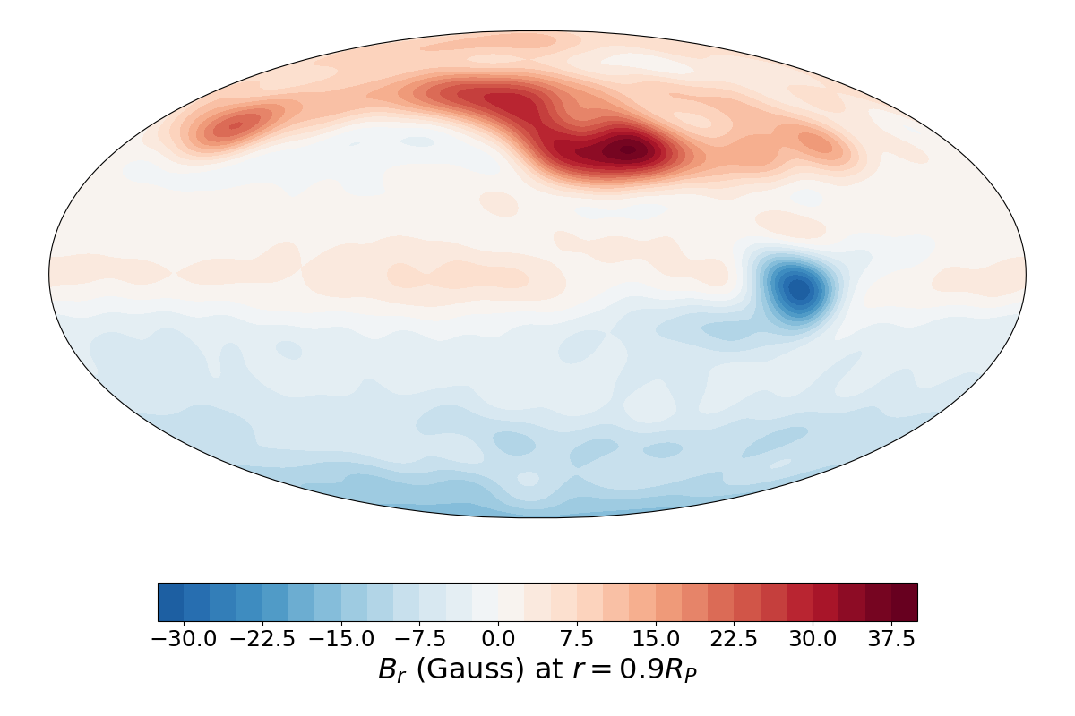
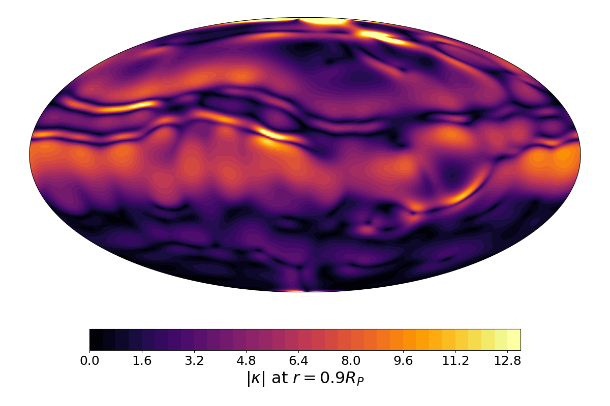
Figure 13: Radial component (top) and curvature modulus (bottom) of Jupiter’s magnetic field at 0.9 planetary radius in the Mollweide projection, reconstructed with the model JRM33 ($n_{\rm max}=13$).

The curvature of the magnetic field is defined as $\boldsymbol{\kappa}=(\boldsymbol{b}\cdot\boldsymbol{\nabla})\boldsymbol{b}$, with the corresponding unitary vector field $\boldsymbol{b}=\boldsymbol{B}/|\boldsymbol{B}|$. The mean of the modulus of the curvature at a given radius is,

$$\langle|\boldsymbol{\kappa}(r=r_{\kappa})|\rangle=\frac{\int|\boldsymbol{\kappa}(\theta,\phi;r=r_{\kappa})|\sin\theta d\theta d\phi}{\int\sin\theta d\theta d\phi}\,.$$ (16)

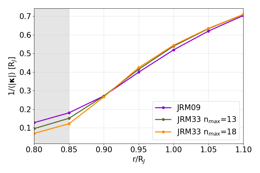
Figure 14: Inverse of the mean curvature modulus for different Jupiter magnetic field models as a function of radius, obtained using a discretized version of equation (16). The JRM33 models do not significantly change if the external multipoles are included.

In Fig. 14, we show the inverse of the mean curvature at different radii for both models, including two different cut-offs for JRM33. The gray zone approximately marks the possible start of the conductive zone where the gradual appearance of metallic hydrogen would prevent the validity of the potential solution. The inverse curvature has a mean value of the order of 10 at a radius of $\sim(0.8-0.9)R_{\rm J}$ (where the dynamo surface should be), which can be taken as a lower limit of the magnetic field curvature inside the Jovian dynamo.

Appendix B MHD dynamo simulations

The code MagIC (Jones et al. 2011; Gastine & Wicht 2012) has been used to solve the MHD equations in a spherical shell under the anelastic approximation with the MESA radial structure as background profiles. We have implemented the radial dependence of density, temperature, gravity, thermal expansion coefficient and the Grüneisen parameter with a very high degree polynomial, fitting them better than $\lesssim 1\%$. We assume constant thermal and viscous diffusivities and we adopt the conductivity profile (and thus a corresponding magnetic diffusivity) first defined in Gómez-Pérez et al. (2010) which consists of an approximately constant conductivity in the hydrogen metallic region joined (at $r=r_{m}$ with $\sigma(r)=\sigma_{m}$) via a polynomial to an exponentially decaying outer molecular region,

$$\tilde{\sigma}(r)=\cases{1}+(\sigma_{m}-1)\left(\dfrac{r-r_{i}}{r_{m}-r_{i}}\right)^{a}\quad\hbox{for}\quad r<r_{m},\\ \sigma_{m}\exp\left[a\left(\dfrac{r-r_{m}}{r_{m}-r_{i}}\right)\dfrac{\sigma_{m}-1}{\sigma_{m}}\right]\quad\hbox{for}\quad r\geq r_{m}.{}$$ (17)

Many works have employed this profile for gas giant convection and dynamo modeling (Duarte et al. 2013, 2018; Wicht et al. 2019b, a; Gastine & Wicht 2021; Yadav et al. 2022) with values of $\sigma_{m}$ and $a$ ranging approximately from 0.9 to 0.01 and from 1 to 25, respectively. In our models, we have arbitrarily chosen $\sigma_{m}=0.6$ and $a=11$, but $r_{m}$ has been chosen as the radius where each MESA structure reaches 100 GPa pressure, as it is the order or magnitude for hydrogen metalization. Due to numerical limitations, dynamo models cannot cover the entire density range of the dynamo region and we have to consider a more limited density contrast (ratio between the innermost and outermost densities) $\rho_{\rm ratio}\lesssim 100$. We thus externally cut the profiles of MESA in order to have a density contrast $\rho_{\rm ratio}$ of either 20 or 100.

For example, for the models shown in Fig. 5, the background MESA profiles correspond to an irradiated $1M_{\rm J}$ planet with internal Ohmic heating at 10 Gyr. At that time, the simulated planetary radius is $1.218R_{\rm J}$, corresponding to an external pressure of and 64 and 5.4 kbar, respectively. We used resolutions of $(N_{r},N_{\theta},N_{\phi})=(193,256,512)$ for the cases with $\rho_{\rm ratio}=20$, and $(N_{r},N_{\theta},N_{\phi})=(241,320,640)$ for the cases with $\rho_{\rm ratio}=100$. In order to explore how sensitive the magnitudes in Fig. 5 are, we vary the Prandtl, magnetic Prandtl, and Rayleigh numbers, the value of $\rho_{\rm ratio}$ and the boundary conditions. Generally speaking, the models shown above reach a steady state dynamo with equatorial jets. More details and the main results of these simulations will be presented in an upcoming paper. For the specific purpose of the current work, we are only interested in the profiles shown in Fig. 5.

References

- Arras & Bildsten (2006) Arras, P. & Bildsten, L. 2006, ApJ, 650, 394
- Balbus & Hawley (2000) Balbus, S. A. & Hawley, J. F. 2000, Space Sci. Rev., 92, 39
- Batygin & Stevenson (2010) Batygin, K. & Stevenson, D. J. 2010, ApJ, 714, L238
- Batygin et al. (2011) Batygin, K., Stevenson, D. J., & Bodenheimer, P. H. 2011, ApJ, 738, 1
- Beltz et al. (2022) Beltz, H., Rauscher, E., Kempton, E. M. R., et al. 2022, AJ, 164, 140
- Benavides et al. (2022) Benavides, S. J., Burns, K. J., Gallet, B., & Flierl, G. R. 2022, ApJ, 938, 92
- Bodenheimer et al. (2001) Bodenheimer, P., Lin, D. N. C., & Mardling, R. A. 2001, ApJ, 548, 466
- Burrows et al. (2007) Burrows, A., Hubeny, I., Budaj, J., & Hubbard, W. B. 2007, ApJ, 661, 502
- Cauley et al. (2019) Cauley, P. W., Shkolnik, E. L., Llama, J., & Lanza, A. F. 2019, Nature Astronomy, 3, 1128
- Chabrier & Baraffe (2007) Chabrier, G. & Baraffe, I. 2007, ApJ, 661, L81
- Cho et al. (2008) Cho, J. Y. K., Menou, K., Hansen, B. M. S., & Seager, S. 2008, ApJ, 675, 817
- Christensen et al. (2009) Christensen, U. R., Holzwarth, V., & Reiners, A. 2009, Nature, 457, 167
- Connerney et al. (2018) Connerney, J. E. P., Kotsiaros, S., Oliversen, R. J., et al. 2018, Geophysical Research Letters, 45, 2590
- Connerney et al. (2022) Connerney, J. E. P., Timmins, S., Oliversen, R. J., et al. 2022, Journal of Geophysical Research: Planets, 127, e2021JE007055, e2021JE007055 2021JE007055
- Debras & Chabrier (2019) Debras, F. & Chabrier, G. 2019, ApJ, 872, 100
- Dietrich et al. (2022) Dietrich, W., Kumar, S., Poser, A. J., et al. 2022, MNRAS[arXiv:2210.03351]
- Dobbs-Dixon & Lin (2008) Dobbs-Dixon, I. & Lin, D. N. C. 2008, ApJ, 673, 513
- Draine et al. (1983) Draine, B. T., Roberge, W. G., & Dalgarno, A. 1983, ApJ, 264, 485
- Duarte et al. (2013) Duarte, L. D., Gastine, T., & Wicht, J. 2013, Physics of the Earth and Planetary Interiors, 222, 22
- Duarte et al. (2018) Duarte, L. D., Wicht, J., & Gastine, T. 2018, Icarus, 299, 206
- Fortney et al. (2021) Fortney, J. J., Dawson, R. I., & Komacek, T. D. 2021, Journal of Geophysical Research (Planets), 126, e06629
- Fortney et al. (2007) Fortney, J. J., Marley, M. S., & Barnes, J. W. 2007, ApJ, 659, 1661
- French et al. (2012) French, M., Becker, A., Lorenzen, W., et al. 2012, ApJS, 202, 5
- Gastine & Wicht (2012) Gastine, T. & Wicht, J. 2012, Icarus, 219, 428
- Gastine & Wicht (2021) Gastine, T. & Wicht, J. 2021, Icarus, 368, 114514
- Ginzburg & Sari (2016) Ginzburg, S. & Sari, R. 2016, ApJ, 819, 116
- Grießmeier et al. (2007) Grießmeier, J. M., Zarka, P., & Spreeuw, H. 2007, A&A, 475, 359
- Guillot et al. (1996) Guillot, T., Burrows, A., Hubbard, W. B., Lunine, J. I., & Saumon, D. 1996, ApJ, 459, L35
- Gómez-Pérez et al. (2010) Gómez-Pérez, N., Heimpel, M., & Wicht, J. 2010, Physics of the Earth and Planetary Interiors, 181, 42
- Hardy et al. (2022) Hardy, R., Cumming, A., & Charbonneau, P. 2022, arXiv e-prints, arXiv:2208.03387
- Heng et al. (2011) Heng, K., Menou, K., & Phillipps, P. J. 2011, MNRAS, 413, 2380
- Heng & Showman (2015) Heng, K. & Showman, A. P. 2015, Annual Review of Earth and Planetary Sciences, 43, 509
- Huang & Cumming (2012) Huang, X. & Cumming, A. 2012, ApJ, 757, 47
- Jones et al. (2011) Jones, C., Boronski, P., Brun, A., et al. 2011, Icarus, 216, 120
- Kao et al. (2016) Kao, M. M., Hallinan, G., Pineda, J. S., et al. 2016, ApJ, 818, 24
- Kao et al. (2018) Kao, M. M., Hallinan, G., Pineda, J. S., Stevenson, D., & Burgasser, A. 2018, ApJS, 237, 25
- Kataria et al. (2015) Kataria, T., Showman, A. P., Fortney, J. J., et al. 2015, ApJ, 801, 86
- Knierim et al. (2022) Knierim, H., Batygin, K., & Bitsch, B. 2022, A&A, 658, L7
- Koll & Komacek (2018) Koll, D. D. B. & Komacek, T. D. 2018, ApJ, 853, 133
- Komacek et al. (2022) Komacek, T. D., Tan, X., Gao, P., & Lee, E. K. H. 2022, ApJ, 934, 79
- Komacek et al. (2020) Komacek, T. D., Thorngren, D. P., Lopez, E. D., & Ginzburg, S. 2020, ApJ, 893, 36
- Komacek & Youdin (2017) Komacek, T. D. & Youdin, A. N. 2017, ApJ, 844, 94
- Kumar et al. (2021) Kumar, S., Poser, A. J., Schöttler, M., et al. 2021, Phys. Rev. E, 103, 063203
- Laughlin et al. (2011) Laughlin, G., Crismani, M., & Adams, F. C. 2011, ApJ, 729, L7
- Li & Goodman (2010) Li, J. & Goodman, J. 2010, ApJ, 725, 1146
- Lorenzen et al. (2011) Lorenzen, W., Holst, B., & Redmer, R. 2011, Phys. Rev. B, 84, 235109
- Parmentier et al. (2013) Parmentier, V., Showman, A. P., & Lian, Y. 2013, A&A, 558, A91
- Paxton et al. (2011) Paxton, B., Bildsten, L., Dotter, A., et al. 2011, ApJS, 192, 3
- Paxton et al. (2013) Paxton, B., Cantiello, M., Arras, P., et al. 2013, ApJS, 208, 4
- Paxton et al. (2019) Paxton, B., Smolec, R., Schwab, J., et al. 2019, ApJS, 243, 10
- Perez-Becker & Showman (2013) Perez-Becker, D. & Showman, A. P. 2013, ApJ, 776, 134
- Perna et al. (2012) Perna, R., Heng, K., & Pont, F. 2012, ApJ, 751, 59
- Perna et al. (2010a) Perna, R., Menou, K., & Rauscher, E. 2010a, ApJ, 719, 1421
- Perna et al. (2010b) Perna, R., Menou, K., & Rauscher, E. 2010b, ApJ, 724, 313
- Rauscher & Menou (2012) Rauscher, E. & Menou, K. 2012, ApJ, 750, 96
- Rauscher & Menou (2013) Rauscher, E. & Menou, K. 2013, ApJ, 764, 103
- Reiners et al. (2009) Reiners, A., Basri, G., & Christensen, U. R. 2009, ApJ, 697, 373
- Reiners & Christensen (2010) Reiners, A. & Christensen, U. R. 2010, A&A, 522, A13
- Rogers & Komacek (2014) Rogers, T. M. & Komacek, T. D. 2014, ApJ, 794, 132
- Rogers & McElwaine (2017) Rogers, T. M. & McElwaine, J. N. 2017, ApJ, 841, L26
- Rogers & Showman (2014) Rogers, T. M. & Showman, A. P. 2014, ApJ, 782, L4
- Sarkis et al. (2021) Sarkis, P., Mordasini, C., Henning, T., Marleau, G. D., & Mollière, P. 2021, A&A, 645, A79
- Saumon et al. (1995) Saumon, D., Chabrier, G., & van Horn, H. M. 1995, ApJS, 99, 713
- Showman et al. (2009) Showman, A. P., Fortney, J. J., Lian, Y., et al. 2009, ApJ, 699, 564
- Showman & Guillot (2002) Showman, A. P. & Guillot, T. 2002, A&A, 385, 166
- Showman et al. (2015) Showman, A. P., Lewis, N. K., & Fortney, J. J. 2015, ApJ, 801, 95
- Soriano-Guerrero et al. (2024) Soriano-Guerrero, C., Viganò, D., & Perna, R. 2024, in prep
- Soriano-Guerrero et al. (2023) Soriano-Guerrero, C., Viganò, D., Perna, R., Akgün, T., & Palenzuela, C. 2023, MNRAS, 525, 626
- Thorngren et al. (2019) Thorngren, D., Gao, P., & Fortney, J. J. 2019, ApJ, 884, L6
- Thorngren & Fortney (2018) Thorngren, D. P. & Fortney, J. J. 2018, AJ, 155, 214
- Tsang & Jones (2020) Tsang, Y.-K. & Jones, C. A. 2020, Earth and Planetary Science Letters, 530, 115879
- Turner et al. (2021) Turner, J. D., Zarka, P., Grießmeier, J.-M., et al. 2021, A&A, 645, A59
- Wang et al. (2015) Wang, J., Fischer, D. A., Horch, E. P., & Huang, X. 2015, ApJ, 799, 229
- Wicht et al. (2019a) Wicht, J., Gastine, T., & Duarte, L. D. V. 2019a, Journal of Geophysical Research (Planets), 124, 837
- Wicht et al. (2019b) Wicht, J., Gastine, T., Duarte, L. D. V., & Dietrich, W. 2019b, A&A, 629, A125
- Wu & Lithwick (2013) Wu, Y. & Lithwick, Y. 2013, ApJ, 763, 13
- Yadav et al. (2022) Yadav, R. K., Cao, H., & Bloxham, J. 2022, The Astrophysical Journal, 940, 185
- Yadav & Thorngren (2017) Yadav, R. K. & Thorngren, D. P. 2017, ApJ, 849, L12
- Yıldız et al. (2024) Yıldız, M., Çelik Orhan, Z., Örtel, S., & Çakır, T. 2024, MNRAS, 528, 6881
- Youdin & Mitchell (2010) Youdin, A. N. & Mitchell, J. L. 2010, ApJ, 721, 1113
- Zaghoo & Collins (2018) Zaghoo, M. & Collins, G. W. 2018, ApJ, 862, 19
- Zaghoo & Silvera (2017) Zaghoo, M. & Silvera, I. F. 2017, Proceedings of the National Academy of Science, 114, 11873
- Zarka (2007) Zarka, P. 2007, Planet. Space Sci., 55, 598