Resolving the $H_{0}$ and $S_{8}$ tensions with neutrino mass and chemical potential

Abstract

A simple and natural extension of the standard $\Lambda$CDM model is to allow relic neutrinos to have non-zero degeneracy. We confront this $\Lambda$CDM$\xi$ model, $\Lambda$CDM with neutrino mass $M_{\nu}$ and degeneracy $\xi_{3}$ as additional parameters, with the Planck TT, lowT, plik–lensing, BAO, and DES datasets, and we observe a strong preference (Bayes factor $\log_{10}B=1.9$) for it over the standard $\Lambda$CDM model. Both the $H_{0}$ and $S_{8}$ tensions are resolved to within 1$\sigma$ with the same set of neutrino parameters, along with 3$\sigma$ evidence for nonzero neutrino mass ($M_{\nu}=0.58^{+0.17}_{-0.13}\ \mathrm{eV}$) and degeneracy ($\xi_{3}=1.27^{+0.42}_{-0.22}$). Furthermore, our analysis favors the scalar index $n_{s}$ to be slightly larger than 1, compatible with some hybrid inflation models, as well as a significantly larger optical depth $\tau$ than the standard Planck value, indicating an earlier onset of reionization.

I Introduction

The recent availability of high precision cosmological and astrophysical data allows for testing cosmological models in unprecedented details. The Lambda Cold Dark Matter ($\Lambda$CDM) model has been very successful in fitting with a wide range of observations [1, 2, 3, 4, 5, 6, 7, 8, 9, 10], though there are discordances between different fitting results. The most notable inconsistency is the Hubble tension, a significant discrepancy between the global and local measurements of the Hubble parameter $H_{0}$. Specifically, there is about 5$\sigma$ disagreement between the result obtained by the Planck collaboration [1], $H_{0}=67.36\pm 0.54\ \ \mathrm{km}\ \mathrm{s}^{-1}\mathrm{Mpc}^{-1}$ at a 68% confidence level (CL) derived from the anisotropies of the cosmic microwave background (CMB) TT, TE, EE, lowT, lowE and plik–lensing data, and that of the SH0ES collaboration [8], $H_{0}=73.04\pm 1.04\ \ \mathrm{km}\ \mathrm{s}^{-1}\mathrm{Mpc}^{-1}$ at a 68% CL measured using Type Ia supernovae calibrated by Cepheids.

There is another milder tension on the strength of matter clustering, quantified by the parameter $S_{8}\equiv\sigma_{8}\sqrt{\Omega_{m}/0.3}$, between the measurements through CMB and weak gravitational lensing and galaxy clustering. Here $\Omega_{m}$ represents the matter density and $\sigma_{8}$ is the standard deviation of matter density fluctuations at radius $8\ h^{-1}\mathrm{Mpc}$ extrapolated to redshift 0 according to linear theory, where $h$ is the dimensionless Hubble parameter. Specifically, there is an approximate 3$\sigma$ discrepancy between $S_{8}=0.832\pm 0.013$ at 68% CL from Planck CMB using TT, TE, EE, lowT, lowE and plik–lensing data [1] and $S_{8}=0.759^{+0.024}_{-0.021}$ from KiDS-1000 weak lensing data [9]. More recently, weak lensing observations from the Hyper Suprime-Cam Subaru Strategic Program (HSC-SSP) indicate a slightly lower tension, ranging from $2-2.5\sigma$ depending on the specific methodologies used [11, 12, 13, 14, 15].

These tensions could suggest the presence of unknown systematic errors in the cosmological data and/or the existence of new physics beyond $\Lambda$CDM. For the latter, a variety of new physics models have been proposed to alleviate both tensions together, such as interacting dark energy (IDE) [16, 17, 18, 19], decaying dark matter (DDM) [20], running vacuum model (RVM) [21], graduated dark energy (gDE) [22, 23], $f(T)$ gravity [24], among others. More detailed discussions on the subject can be found in [25, 26, 27, 28]. Nevertheless, effectively resolving both tensions with the same physics while preserving the successes of $\Lambda$CDM remains challenging.

In this letter, we consider the $\Lambda$CDM + $M_{\nu}$ + $\xi_{i}$ ($\Lambda$CDM$\xi$) model as the minimal extension of the $\Lambda$CDM model, with $M_{\nu}\equiv\sum_{i}m_{i}$ and $\xi_{i}\equiv\mu_{i}/T_{\nu}$ being the neutrino mass and degeneracy parameters, respectively, where $m_{i}$ and $\mu_{i}$ denote the mass eigenvalue and chemical potential of the $i^{th}$ neutrino mass eigenstate, respectively, and $T_{\nu}$ is the relic neutrino temperature. Hereafter, following the convention in [1], $\Lambda$CDM means the standard cosmological model with fixing $M_{\nu}=0.06\ \mathrm{eV}$ and $\xi_{i}=0$. While the electron-type neutrino degeneracy parameter $\xi_{e}\ll 1$ is tightly constrained by Big Bang nucleosynthesis (BBN) [29, 30], the possibility of $\mathcal{O}(1)$ degeneracy parameters for muon-type and tau-type neutrinos, $\nu_{\mu},\nu_{\tau}$, remains open. Previous studies [31, 32] have shown that nonzero $\xi_{i}$ can help alleviate the $H_{0}$ tension. Our key result is shown as the blue contours in Figure 1. By fitting with the Planck TT, lowT, plik–lensing [1], Baryonic Acoustic Oscillation (BAO) [33, 34, 35] and Dark Energy Survey (DES) [36] data, we can resolve both the $H_{0}$ and $S_{8}$ tensions with the same set of neutrino parameters using the $\Lambda$CDM$\xi$ model. Furthermore, there is a 3$\sigma$ evidence for nonzero neutrino mass ($M_{\nu}=0.58^{+0.17}_{-0.13}$ eV) and degeneracy ($\xi_{3}=1.27^{+0.42}_{-0.22}$). Our mean values for the scalar index $n_{s}$ and CMB optical depth $\tau$ differ significantly from the standard Planck values, which have profound implications for our understanding of the early universe.

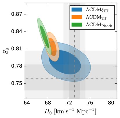
Figure 1: 2D contours (for 68% CL and 95% CL) for $H_{0}$ and $S_{8}$. The Planck results for $\Lambda$CDM fitting are denoted as $\Lambda\mathrm{CDM}_{\mathrm{Planck}}$, shown as green contours, incorporating Planck TT, TE, EE, lowT, lowE and plik–lensing data. The orange and blue contours correspond to the $\Lambda\mathrm{CDM}_{\mathrm{TT}}$ and $\Lambda\mathrm{CDM}\xi_{\mathrm{TT}}$ models, respectively, using Planck TT, lowT, plik–lensing, BAO, and DES data. The grey regions represent the 68% and 95% CL for $H_{0}$ obtained from SH0ES [8] and for $S_{8}$ from KiDS [9], respectively.

II Methodology

As shown in [37], the neutrino degeneracy becomes diagonal in the mass eigen basis just before neutrino decoupling, and $\xi_{i}$ can be related to $\xi_{\alpha}$ in the flavor basis by the Pontecorvo–Maki–Nakagawa–Sakata (PMNS) matrix (e.g., Eq. (13) in [37]), where $\alpha=e,\mu,\tau$. Based on strong constraints from BBN [29, 30] and the strong mixing between $\nu_{\mu}$ and $\nu_{\tau}$, we assume $\xi_{e}=0$ and $\xi_{\mu}=\xi_{\tau}$. Then we are left with only one free parameter related to neutrino degeneracy, which we choose to be $\xi_{3}$.

The neutrino degeneracy parameters enter the CMB anisotropy calculation through the neutrino energy density,

$$\rho_{\nu}=\frac{1}{2\uppi^{2}}\sum_{i=1}^{3}\int_{0}^{\infty}\left[\frac{\sqrt{p^{2}+m_{i}^{2}}}{e^{p/T_{\nu}-\xi_{i}}+1}+\frac{\sqrt{p^{2}+m_{i}^{2}}}{e^{p/T_{\nu}+\xi_{i}}+1}\right]p^{2}dp,$$ (1)

which plays a role in the expansion history of the universe and the Boltzmann equations. Following [32], we modified CAMB [38, 39] to include these effects in the calculations of the CMB anisotropy power spectra. For more details, please refer to [32]. In this letter, we compare the fitting of cosmological data with two models: $\Lambda$CDM model (with $M_{\nu}=0.06\ \mathrm{eV}$ and $\xi_{3}=0$) and $\Lambda$CDM$\xi$ model, in which $M_{\nu}$ and $\xi_{3}$ are allowed to vary.

For the standard Planck data combination, including high-multipole ($l>30$) Planck CMB temperature and polarization anisotropy power spectra (TT, TE, EE) from Planck likelihood plik, low-multipole ($2\leq l\leq 30$) temperature power spectrum (lowT) from Commander, low-multipole ($2\leq l\leq 30$) polarization power spectrum (lowE) from SimAll and the CMB lensing data (plik–lensing) [1], the results for $\Lambda$CDM ($\Lambda\mathrm{CDM}_{\mathrm{Planck}}$) are shown as the green contours in Figure 1, which is the standard Planck result [1]. Both $H_{0}$ and $S_{8}$ are in clear tension with those from SH0ES [8] and KiDS [9], respectively.

The $\Lambda\mathrm{CDM}_{\mathrm{Planck}}$ constraints on the optical depth $\tau$ come mainly from the lowE data. However, it is about 2$\sigma$ deviated from that measured by the Atacama Cosmology Telescope (ACT) CMB temperature and polarization combined with BAO data [40]. Also, as discussed in [1], only the CMB temperature spectrum can agree well for two different Planck likelihoods plik and CamSpec. Therefore, we will only use the temperature data (TT+lowT) and plik–lensing from CMB. In addition, the neutrino parameters can be better constrained if we include the BAO data from BOSS DR12 “LOWZ” and “CMASS” surveys [35], 6dF Galaxy Survey [33], DR7 Main Galaxy Sample (MGS) [34], and DES data from the Dark Energy Survey [36].

We denote the fitting results of the above data with models $\Lambda$CDM and $\Lambda$CDM$\xi$ by $\Lambda\mathrm{CDM}_{\mathrm{TT}}$ and $\Lambda\mathrm{CDM}\xi_{\mathrm{TT}}$, respectively. We use CosmoMC [41, 42] to perform Markov Chain Monte Carlo (MCMC) fitting to get the posterior distributions of the cosmological and neutrino parameters.

III Results

III.1 $H_{0}$ and $S_{8}$

Our main results are summarized in Table 1. With $\Lambda\mathrm{CDM}_{\mathrm{TT}}$, we obtain:

$$\left.\begin{aligned} H_{0}&=68.79\pm 0.56\ \mathrm{km}\ \mathrm{s^{-1}}\ \mathrm{Mpc}^{-1},\\ S_{8}&=0.813\pm 0.010.\end{aligned}\right\}68\%\ \mathrm{CL}$$ (2)

Moreover, we calculate the deviations (in unit of standard deviations), $n_{\sigma}(H_{0})=3.6$ and $n_{\sigma}(S_{8})=2.2$, from the mean values of $H_{0}$ and $S_{8}$ from the SH0ES ($H_{0}=73.04\pm 1.04\ \mathrm{km}\ \mathrm{s^{-1}}\ \mathrm{Mpc}^{-1}$) [10] and KiDS results ($S_{8}=0.759^{+0.024}_{-0.021}$) [9], respectively, using the Marginalised Posterior Compatibility Level (MPCL) [28], where we treat the latter as Gaussian distributions. We can see that there are still significant tensions in both $H_{0}$ and $S_{8}$, only slightly better than those of $\Lambda\mathrm{CDM}_{\mathrm{Planck}}$, with $n_{\sigma}(H_{0})=4.9$ and $n_{\sigma}(S_{8})=2.8$.

For $\Lambda$CDM$\xi_{\mathrm{TT}}$, we have

$$\left.\begin{aligned} H_{0}&=71.27^{+1.97}_{-2.04}\ \mathrm{km}\ \mathrm{s^{-1}}\ \mathrm{Mpc}^{-1},\\ S_{8}&=0.787\pm 0.014,\end{aligned}\right\}68\%\ \mathrm{CL}$$ (3)

with $n_{\sigma}(H_{0})=0.8$ and $n_{\sigma}(S_{8})=1.1$. Both the $H_{0}$ and $S_{8}$ tensions are resolved with the same set of mean values of $M_{\nu}$ and $\xi_{3}$.

We compare the models by the Bayes factor $B$:

$$B=\frac{K({\Lambda\mathrm{CDM}}_{\mathrm{TT}})}{K({\Lambda\mathrm{CDM}\xi}_{\mathrm{TT}})},$$ (4)

where $K$ is the Bayesian evidence calculated using MCEvidence [43]. We obtain $\log_{10}B=1.9$, meaning that the $\Lambda$CDM$\xi$ model is strongly preferred to $\Lambda$CDM by the cosmological data we used. The mean values of all cosmological parameters with 68% CL are summarized in Table 2 of the Supplemental Materials.

	$M_{\nu}$ [eV]	$\xi_{3}$	$H_{0}\ [\mathrm{km}\ \mathrm{s^{-1}}\ \mathrm{Mpc}^{-1}]$	$n_{\sigma}(H_{0})$	$S_{8}$	$n_{\sigma}(S_{8})$	$\ln K$
$\Lambda\mathrm{CDM}_{\mathrm{Planck}}$	$0.06$	$0$	$68.36\pm 0.54$	$4.9$	$0.832\pm 0.013$	$2.8$	—
$\Lambda\mathrm{CDM}_{\mathrm{TT}}$	$0.06$	$0$	$68.79\pm 0.56$	$3.6$	$0.813\pm 0.010$	$2.2$	$-691.7$
$\Lambda$CDM$\xi_{\mathrm{TT}}$	$0.58^{+0.17}_{-0.13}$	$1.27^{+0.42}_{-0.22}$	$71.27^{+1.97}_{-2.04}$	$0.8$	$0.787\pm 0.014$	$1.1$	$-687.3$

Table 1: Mean values (68% CL) for $M_{\nu}$, $\xi_{3}$, $H_{0}$ and $S_{8}$ and their deviations (in unit of $\sigma$) $n_{\sigma}$ with respect to the corresponding ‘tension’ measurements. $\ln K$ is the Bayesian evidence.

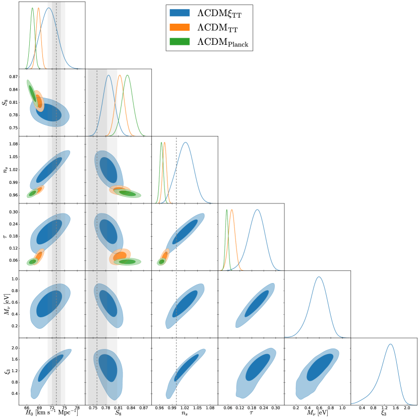
Figure 2: Same as Figure 1, but for more selected cosmological and neutrino parameters, together with 1D marginalized posterior PDFs. The dashed line in panels for $n_{s}$ indicates $n_{s}=1$.

III.2 Other parameters

Figure 2 shows the marginalized posterior 1D PDFs and 2D contours for different cosmological parameters for ${\Lambda\mathrm{CDM}}_{\mathrm{Planck}}$ (green), ${\Lambda\mathrm{CDM}}_{\mathrm{TT}}$ (orange), and ${\Lambda\mathrm{CDM}\xi}_{\mathrm{TT}}$ (blue).

III.2.1 neutrino properties: $M_{\nu}$ and $\xi_{3}$

For the fitting result of $\Lambda$CDM$\xi_{\mathrm{TT}}$, we find that cosmological data prefer $M_{\nu}=0.58^{+0.17}_{-0.13}\ \mathrm{eV}$, $\xi_{3}=1.27^{+0.42}_{-0.22}$ (68%), with a 2.8$\sigma$ (2.9$\sigma$) evidence for the nonzero $M_{\nu}$ ($\xi_{3}$). The blue contours of Figure 2 show that both the nonzero values of $M_{\nu}$ and $\xi_{3}$ help to increase $H_{0}$ and decrease $S_{8}$.

The sound horizon angular size $\theta_{\mathrm{MC}}=r_{s}/D_{M}$ at photon decoupling ($z_{*}$) is constrained very well by the CMB data, where $r_{s}$ and $D_{M}$ are the comoving sound horizon and distance to the last scattering, respectively. We can understand the correlations between $H_{0}$ and $M_{\nu}$ and $H_{0}$ and $\xi_{3}$ in fitting the CMB data by a perturbative approach [32] (see Supplemental Materials for details). A small variation of $M_{\nu}$ around a reference value $M_{\nu}^{\mathrm{ref}}$ would induce corresponding variations in $r_{s}$ and $D_{M}$. We assume that $H_{0}$ is varied accordingly so as to keep $\theta_{\mathrm{MC}}$ unchanged (fixed to the observed value). We therefore obtain,

$$C_{H}\frac{H_{0}-H_{0}^{\mathrm{ref}}}{H_{0}^{\mathrm{ref}}}=C_{m}\frac{M_{\nu}-M_{\nu}^{\mathrm{ref}}}{M_{\nu}^{\mathrm{ref}}},$$ (5)

where $C_{H}$ and $C_{m}$ can be calculated using the expressions for $r_{s}$ and $D_{M}$. Similarly, we obtain the correlation between $H_{0}$ and $\xi_{i}$ by fixing $M_{\nu}$ together with $\theta_{\mathrm{MC}}$ and all other cosmological parameters:

$$C_{H}\frac{H_{0}-H_{0}^{\mathrm{ref}}}{H_{0}^{\mathrm{ref}}}=\sum_{i}C_{\xi,i}^{1}(\xi_{i}-\xi_{i}^{\mathrm{ref}})+\sum_{i}C_{\xi,i}^{2}(\xi_{i}-\xi_{i}^{\mathrm{ref}})^{2}.$$ (6)

The coefficients $C_{H},C_{m},C_{\xi,i}^{1},C_{\xi,i}^{2}$ are listed in Table 3 of Supplemental Materials. These semi-analytic results are shown in Figure 3, which agree well with the MCMC results. Moreover, we can obtain roughly the same 95% contours in the MCMC when the BAO data is included (see Supplemental Materials for details).

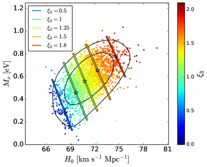
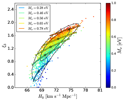
Figure 3: PDFs for $H_{0}$ and $M_{\nu}$ ($\xi_{3}$), with scatter points colored according to values of $\xi_{3}$ ($M_{\nu}$) in the top (bottom) panel. The colored lines are from Eqs. (5) and (6), with stars representing the corresponding reference points.

From the $\Lambda$CDM$\xi_{\mathrm{TT}}$ fitting results, we find a larger $\Omega_{b}h^{2}$ ($0.02325^{+0.00040}_{-0.00037}$, 68% CL), compared with $\Omega_{b}h^{2}=0.02242\pm 0.00020$ from $\Lambda\mathrm{CDM}_{\mathrm{TT}}$. Based on this, we show in the Supplemental Materials that the BBN data also prefers $\xi_{3}=1.22$, which is consistent with our findings here.

III.2.2 scalar index $n_{s}$

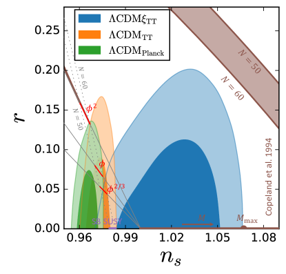
Figure 4: Same as Figure 1 but for the $n_{s}-r$ contours and several selected inflation models’ predictions, shown as red, purple and brown lines, with uncertainties in the number of e-folds of $50<N<60$ (more details can be found in the main text). $M_{\mathrm{max}}$ is the upper bound of the model parameter $M$ in [44].

The mean value of $n_{s}$ in $\Lambda\mathrm{CDM}\xi_{\mathrm{TT}}$ ($n_{s}=1.020^{+0.020}_{-0.019}$ 68% CL) is consistent with 1 and 3.1$\sigma$ (MPCL) larger than that of $\Lambda\mathrm{CDM}_{\mathrm{Planck}}$ ($n_{s}=0.9649\pm 0.0042$ 68% CL). This may have important implications on inflation models.

To quantify the implications of our results on inflation models, we vary one more parameter, the scalar-to-tensor ratio $r$, when fitting the TT data. The mean contours of $n_{s}-r$ are shown in Figure 4. The brown curve shows one of the simplest hybrid models of [44], with the number of e-folds $N$ between 50 and 60, where the energy density during inflation is dominated by the potential composed of two scalar fields $\phi$ and $\psi$,

$$V(\phi,\psi)=\frac{1}{4}\lambda(\psi^{2}-M^{2})^{2}+\frac{1}{2}m^{2}\phi^{2}+\frac{1}{2}\lambda^{\prime}\phi^{2}\psi^{2},$$ (7)

where we take $\lambda=\lambda^{\prime}=1$ following [45] and fix the primordial perturbation amplitude $A_{s}$ according to our CMB fitting results [44], so that we are left with only one parameter $M$ (or $m$). We obtain the upper bound for $M$ ($M_{\mathrm{max}}$) (or $m$ ($m_{\mathrm{max}}$)) around $1\times 10^{-4}\ m_{\mathrm{Pl}}$ ($1\times 10^{-8}\ m_{\mathrm{Pl}}$), where $m_{\mathrm{Pl}}\equiv\sqrt{\hbar c/G}$ is the Planck mass. Moreover, other hybrid models, such as discussed in [46, 44, 45], can also be compatible with the results of $\Lambda\mathrm{CDM}\xi_{\mathrm{TT}}$. Furthermore, another kind of hybrid models, spontaneously broken supersymmetric (SB SUSY) theories [47], as shown in purple in Figure 4, is compatible with both $\Lambda\mathrm{CDM}_{\mathrm{TT}}$ and $\Lambda\mathrm{CDM}\xi_{\mathrm{TT}}$. For all the above models, our results suggest a very small value of $r$. We also show monomial potential models $V(\phi)\sim\phi^{p}$, with $p=$ 2, 1 and 2/3 as red lines ($50<N<60$) in Figure 4 for comparison [48, 49, 50, 51].

III.2.3 optical depth $\tau$

The mean value of the CMB optical depth from $\Lambda$CDM$\xi_{\mathrm{TT}}$ ($\tau=0.202^{+0.044}_{-0.036}$) is 3.4$\sigma$ (MPCL) larger than from $\Lambda$CDM_Planck ($\tau=0.0544\pm 0.0073$). For $\tau\approx 0.2$, we can estimate the reionization redshift to be $z\approx 20$ (see, e.g., Eq. (2) in [52]). This high reionization redshift may in fact be consistent with the recent JWST observation of high-redshift objects [53, 54, 55, 56, 57].

IV Conclusion

In this letter, we fit Planck TT, lowT, plik–lensing, BAO and DES data with the $\Lambda$CDM and $\Lambda$CDM$\xi$ models. We find that the $\Lambda$CDM$\xi$ model is strongly preferred.

Our main results are:

(i) Both the $H_{0}$ and $S_{8}$ tensions are resolved with the same set of neutrino parameters. In particular, the global and local measurements of $H_{0}$ and $S_{8}$ agree to about 1$\sigma$.

(ii) There are around 3$\sigma$ evidences for both neutrino mass $M_{\nu}=0.58^{+0.17}_{-0.13}\ \mathrm{eV}$ (68% CL) and degeneracy parameter $\xi_{3}=1.27^{+0.42}_{-0.22}$ (68% CL), respectively. Moreover, this $\mathcal{O}(1)$ neutrino degeneracy parameter is also consistent with the BBN data.

(iii) The mean value of the scalar index $n_{s}\gtrsim 1$ and is compatible with some hybrid inflation models.

(iv) The mean value of the CMB optical depth $\tau$ is much larger than the standard Planck result, suggesting an earlier onset of reionization, to $z\approx 20$.

Upcoming CMB observations, such as those from the South Pole Telescope (SPT-3G) [58], ACT [59], Simons Observatory [60], CMB-S4 [61, 62], the proposed CMB-HD [63, 64, 65], and other future missions could provide further tests of this $\Lambda$CDM$\xi$ model and more precise measurements of the neutrino parameters.

V Supplemental Materials

V.1 Full parameter table

Table 2 shows all cosmological parameters with 68% CL from $\Lambda\mathrm{CDM}_{\mathrm{Planck}}$, $\Lambda\mathrm{CDM}_{\mathrm{TT}}$, and $\Lambda\mathrm{CDM}\xi_{\mathrm{TT}}$, and we follow the definitions of the cosmological parameters as shown in Table 1 of [70]. The first group shows the free parameters used in each case, while the second group denotes the derived parameters based on the first group.

Parameter	$\Lambda\mathrm{CDM}_{\mathrm{Planck}}$	$\Lambda\mathrm{CDM}_{\mathrm{TT}}$	$\Lambda\mathrm{CDM}\xi_{\mathrm{TT}}$
$\Omega_{b}h^{2}$	$0.02237\pm 0.00015$	$0.02242\pm 0.00020$	$0.02325^{+0.00040}_{-0.00037}$
$\Omega_{c}h^{2}$	$0.1200\pm 0.0012$	$0.1166\pm 0.0012$	$0.1225^{+0.0046}_{-0.0048}$
$100\theta_{\mathrm{MC}}$	$1.04092\pm 0.00031$	$1.04119\pm 0.00042$	$1.04056\pm 0.00058$
$\tau$	$0.0544\pm 0.0073$	$0.079^{+0.017}_{-0.016}$	$0.202^{+0.044}_{-0.036}$
$\ln(10^{10}A_{s})$	$3.044\pm 0.014$	$3.085^{+0.031}_{-0.030}$	$3.339^{+0.092}_{-0.075}$
$n_{s}$	$0.9649\pm 0.0042$	$0.9721\pm 0.0046$	$1.020^{+0.021}_{-0.019}$
$M_{\nu}$	—	—	$0.58^{+0.17}_{-0.13}$
$\xi_{3}$	—	—	$1.27^{+0.42}_{-0.22}$
$H_{0}[\mathrm{km}\ \mathrm{s}^{-1}\ \mathrm{Mpc}^{-1}]$	$67.36\pm 0.54$	$68.79\pm 0.56$	$71.3\pm 2.0$
$\Omega_{\Lambda}$	$0.6847\pm 0.0073$	$0.7048\pm 0.0069$	$0.6976\pm 0.0085$
$\Omega_{m}$	$0.3153\pm 0.0073$	$0.2952\pm 0.0069$	$0.3024\pm 0.0085$
$\Omega_{m}h^{2}$	$0.1430\pm 0.0011$	$0.1396\pm 0.0011$	$0.1536^{+0.0071}_{-0.0074}$
$\Omega_{m}h^{3}$	$0.09633\pm 0.00030$	$0.09605^{+0.00045}_{-0.00046}$	$0.1096^{+0.0074}_{-0.0085}$
$\sigma_{8}$	$0.8111\pm 0.0060$	$0.820\pm 0.010$	$0.784\pm 0.017$
$S_{8}\equiv\sigma_{8}(\Omega_{m}/0.3)^{0.5}$	$0.832\pm 0.013$	$0.813\pm 0.010$	$0.787\pm 0.014$
$\sigma_{8}\Omega_{m}^{0.25}$	$0.6078\pm 0.0064$	$0.6044\pm 0.0069$	$0.581\pm 0.011$
$z_{re}$	$7.67\pm 0.73$	$9.9^{+1.5}_{-1.3}$	$19.4^{+3.2}_{-2.4}$
$10^{9}A_{s}$	$2.100\pm 0.030$	$2.187^{+0.067}_{-0.066}$	$2.83\pm 0.24$
$10^{9}A_{s}e^{-2\tau}$	$1.883\pm 0.011$	$1.866\pm 0.011$	$1.882\pm 0.018$
Age[Gyr]	$13.797\pm 0.023$	$13.764\pm 0.029$	$13.21^{+0.32}_{-0.34}$
$z_{*}$	$1089.92\pm 0.25$	$1089.55\pm 0.30$	$1090.02^{+0.50}_{-0.60}$
$r_{*}$[Mpc]	$144.43\pm 0.26$	$145.29\pm 0.30$	$139.0^{+3.2}_{-3.5}$
$100\theta_{*}$	$1.04110\pm 0.00031$	$1.04139\pm 0.00041$	$1.04044^{+0.00072}_{-0.00078}$
$z_{\mathrm{drag}}$	$1059.94\pm 0.30$	$1059.81\pm 0.45$	$1062.9^{+1.5}_{-1.4}$
$r_{\mathrm{drag}}$[Mpc]	$147.09\pm 0.26$	$147.96\pm 0.33$	$141.3^{+3.4}_{-3.7}$
$k_{\mathrm{D}}\mathrm{[Mpc^{-1}]}$	$0.14087\pm 0.00030$	$0.13999\pm 0.00042$	$0.1449^{+0.0027}_{-0.0028}$
$z_{\mathrm{eq}}$	$3402\pm 26$	$3321\pm 27$	$3482^{+117}_{-123}$
$k_{\mathrm{eq}}\mathrm{[Mpc^{-1}]}$	$0.010384\pm 0.000081$	$0.010137^{+0.000083}_{-0.000082}$	$0.01095^{+0.00052}_{-0.00055}$
$100\theta_{\mathrm{s,eq}}$	$0.4594\pm 0.0026$	$0.4572\pm 0.0027$	$0.439^{+0.012}_{-0.013}$

Table 2: Mean values of cosmological parameters (68% CL) for $\Lambda\mathrm{CDM}_{\mathrm{Planck}}$, $\Lambda\mathrm{CDM}_{\mathrm{TT}}$ and $\Lambda\mathrm{CDM}\xi_{\mathrm{TT}}$. The first group lists free parameters used in each case, while the second group shows the derived parameters based on the first group.

V.2 Consistency with BBN

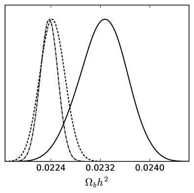
Figure 5: Posterior distribution of baryon density $\Omega_{b}h^{2}$ obtained from $\Lambda\mathrm{CDM}_{\mathrm{Plnack}}$ (dash-dotted), $\Lambda\mathrm{CDM}_{\mathrm{TT}}$ (dashed), and $\Lambda$CDM$\xi_{\mathrm{TT}}$ (solid).

As shown in Figure 5 or Table 2, for the cosmological baryon density, we obtain $\Omega_{b}h^{2}=0.02325^{+0.00040}_{-0.00037}$ 68% C.L. from $\Lambda\mathrm{CDM}\xi_{\mathrm{TT}}$. Our result is significantly larger than that from $\Lambda\mathrm{CDM}_{\mathrm{TT}}$ ($\Omega_{b}h^{2}=0.02242\pm 0.00020$).

To estimate the implication of a larger $\Omega_{b}h^{2}$ on BBN, we adopt the following fitting formulae [71],

$$\frac{\Delta Y_{p}}{\overline{Y_{p}}} =0.04\frac{\Delta\Omega_{b}h^{2}}{\overline{\Omega_{b}h^{2}}}+0.16\frac{\Delta N_{\nu}}{3.0}-0.96\xi_{\nu_{e}},$$ (8)

$$\frac{\Delta\mathrm{D}/\mathrm{H}}{\overline{\mathrm{D}/\mathrm{H}}} =-1.65\frac{\Delta\Omega_{b}h^{2}}{\overline{\Omega_{b}h^{2}}}+0.41\frac{\Delta N_{\nu}}{3.0}-0.53\xi_{\nu_{e}}.$$

The bars over the symbols represent the corresponding reference values used in [71]. To keep the measured quantities of BBN unchanged, i.e., the LHS of Eq. (8) equals zero, but the baryon density $\Omega_{b}h^{2}$ changes from the reference value 0.02225 to 0.02325 (i.e., $\overline{\Omega_{b}h^{2}}=0.02225$ and $\Delta\Omega_{b}h^{2}=0.02325-0.02225$), we obtian $\Delta N_{\nu}=0.71$ and $\xi_{\nu_{e}}=0.04$. During the BBN period, neutrinos are relativistic particles, so we have

$$\Delta N_{\nu}=\frac{15}{7}\sum_{i}\left(\frac{\xi_{i}}{\uppi}\right)^{2}\left[2+\left(\frac{\xi_{i}}{\uppi}\right)^{2}\right].$$ (9)

We thus obtain

$$\xi_{1} =-0.05,$$ (10)

$$\xi_{2} =0.14,$$

$$\xi_{3} =1.22.$$

This result is consistent with our results in the main text.

V.3 Semi-analytic model on $H_{0}$

V.3.1 Perturbation analysis of $\theta_{\mathrm{MC}}$

In this section, following [32], we use a semi-analytic approach to understand the neutrino effects on $H_{0}$. We start from the sound horizon angular size ($\theta_{\mathrm{MC}}$) at the epoch of photon decoupling $z_{*}$,

$$\theta_{\mathrm{MC}}=\frac{r_{s}}{D_{M}},$$ (11)

where $r_{s}$ and $D_{M}$ are the comoving sound horizon and distance to the last scattering, respectively,

$$r_{s}(z_{*}) =\int_{z_{*}}^{\infty}\frac{dz}{\sqrt{3(1+R)}H(z)},$$ (12)

$$D_{M}(z_{*}) =\int_{0}^{z_{*}}\frac{dz}{H(z)},$$

where $R\equiv 3\rho_{b}/4\rho_{\gamma}$ is the ratio between baryon and photon energy densities.

For convenience, we take $c=\hbar=k_{B}=1$ and define the following kernels

$$G(x,\xi_{i}) \equiv\frac{1}{e^{x-\xi_{i}}+1}+\frac{1}{e^{x+\xi_{i}}+1},$$ (13)

$$F(x,\xi_{i}) \equiv\frac{1}{e^{x-\xi_{i}}+1}-\frac{1}{e^{x+\xi_{i}}+1},$$

$$K_{1}(x,y) =2x\sqrt{x^{2}+y^{2}}+\frac{x^{3}}{\sqrt{x^{2}+y^{2}}},$$

$$K_{2}(x,y) =2\sqrt{x^{2}+y^{2}}+\frac{5x^{2}}{\sqrt{x^{2}+y^{2}}}-\frac{x^{4}}{(x^{2}+y^{2})^{3/2}},$$

and functionals

$$\mathcal{I}_{r}[f(z)] \equiv\int_{z_{*}}^{\infty}\frac{f(z)}{[H^{\mathrm{ref}}(z)]^{3}}\frac{dz}{\sqrt{3(1+R)}},$$ (14)

$$\mathcal{I}_{D}[f(z)] \equiv\int_{0}^{z_{*}}\frac{f(z)}{[H^{\mathrm{ref}}(z)]^{3}}dz.$$

As $\theta_{\mathrm{MC}}$ is well constrained by CMB data, we expand $r_{s}$ and $D_{M}$ around reference values of $M_{\nu}$ and $H_{0}$, denoted as $M_{\nu}^{\mathrm{ref}}$ and $H_{0}^{\mathrm{ref}}$, to the lowest order by fixing $\theta_{\mathrm{MC}}$, $\xi_{i}$ and other cosmological parameters ($\Omega_{b}h^{2},\Omega_{c}h^{2},\Omega_{\gamma}h^{2}$). We get,

$$C_{H}\frac{H_{0}-H_{0}^{\mathrm{ref}}}{H_{0}^{\mathrm{ref}}}=C_{m}\frac{M_{\nu}-M_{\nu}^{\mathrm{ref}}}{M_{\nu}^{\mathrm{ref}}},$$ (15)

where

$$C_{H} =\mathcal{I}_{r}(1)-\theta_{\mathrm{MC}}\mathcal{I}_{D}(1),$$ (16)

$$C_{m} =\theta_{\mathrm{MC}}\mathcal{I}_{D}[C_{\rho m}(z)-(1+z)^{3}C_{\rho m}(0)]$$

$$-\mathcal{I}_{r}[C_{\rho m}(z)-(1+z)^{3}C_{\rho m}(0)],$$

$$\small C_{\rho m}(z)=\frac{T_{\nu 0}^{4}(1+z)^{2}}{4\uppi^{2}\rho_{\mathrm{crit},0}^{\mathrm{ref}}}\int_{0}^{\infty}dx\sum_{i}G(x,\xi_{i})\frac{x^{2}\tilde{m}^{2}_{i}}{\sqrt{x^{2}+(\tilde{m}_{i}/(1+z))^{2}}},$$ (17)

and $\tilde{m}_{i}\equiv m_{i}/T_{\nu 0}$. $T_{\nu 0}$ and $\rho_{\mathrm{crit},0}$ are the relic neutrino temperature and critical energy density of the Universe today, respectively.

Similarly, we expand around $\xi_{i}^{\mathrm{ref}}$ ($i=1,2,3$) and $H_{0}^{\mathrm{ref}}$ to investigate the correlation between $\xi_{i}$ and $H_{0}$, while for $\xi_{i}$, we keep up to the second order term,

where

$$C_{\xi,i}^{1} =\theta_{\mathrm{MC}}\mathcal{I}_{D}[C_{\rho\xi,i}^{1}(z)-(1+z)^{3}C_{\rho\xi,i}^{1}(0)]$$ (19)

$$-\mathcal{I}_{r}[C_{\rho\xi,i}^{1}(z)-(1+z)^{3}C_{\rho\xi,i}^{1}(0)],$$

$$C_{\xi,i}^{2} =\theta_{\mathrm{MC}}\mathcal{I}_{D}[C_{\rho\xi,i}^{2}(z)-(1+z)^{3}C_{\rho\xi,i}^{2}(0)]$$

$$-\mathcal{I}_{r}[C_{\rho\xi,i}^{2}(z)-(1+z)^{3}C_{\rho\xi,i}^{2}(0)],$$

$$C_{\rho\xi,i}^{1}(z) =\frac{T_{\nu 0}^{4}(1+z)^{4}}{4\uppi^{2}\rho_{\mathrm{crit},0}^{\mathrm{ref}}}\int_{0}^{\infty}dxK_{1}(x,\tilde{m}_{i}/(1+z))F(x,\xi_{i}),$$ (20)

$$C_{\rho\xi,i}^{2}(z) =\frac{T_{\nu 0}^{4}(1+z)^{4}}{8\uppi^{2}\rho_{\mathrm{crit},0}^{\mathrm{ref}}}\int_{0}^{\infty}dxK_{2}(x,\tilde{m}_{i}/(1+z))G(x,\xi_{i}).$$

We can find from above that, when $\xi_{i}$ approaches zero, $F(x,\xi_{i})\rightarrow 0$, then $C_{\rho\xi,i}^{1}$ also approaches zero, causing the first-order coefficient ($C_{\xi,i}^{1}$) to become negligible and allowing the second-order perturbation term to dominate. Conversely, when $\xi_{i}\sim\mathcal{O}(1)$, the first-order term takes precedence. Therefore, unlike $M_{\nu}$, it is necessary to terms up to second order in $\xi_{i}$.

$\xi_{3}^{\mathrm{ref}}$	0.5	1	1.25	1.5	1.8
$M_{\nu}^{\mathrm{ref}}$ [eV]	0.28	0.46	0.56	0.65	0.78
$H_{0}^{\mathrm{ref}}\ [\mathrm{km}\ \mathrm{s}^{-1}\ \mathrm{Mpc}^{-1}]$	68.4	69.7	70.8	72.4	74.6
$C_{m}/C_{H}$	-0.023	-0.037	-0.046	-0.055	-0.067
$C_{\xi,1}^{1}/C_{H}$	-0.005	-0.010	-0.012	-0.015	-0.018
$C_{\xi,2}^{1}/C_{H}$	0.006	0.011	0.014	0.017	0.021
$C_{\xi,3}^{1}/C_{H}$	0.075	0.151	0.191	0.231	0.279
$C_{\xi,1}^{2}/C_{H}$	0.073	0.069	0.066	0.062	0.058
$C_{\xi,2}^{2}/C_{H}$	0.073	0.069	0.066	0.063	0.058
$C_{\xi,3}^{2}/C_{H}$	0.078	0.090	0.098	0.106	0.117

Table 3: Selected expansion reference points and calculated coefficients of Eqs. (16) and (19).

We choose five $\xi_{3}^{\mathrm{ref}}$ points, and obtain the corresponding $M_{\nu}^{\mathrm{ref}}$ and $H_{0}^{\mathrm{ref}}$ from the mean values in MCMC chains with fixing $\xi_{3}^{\mathrm{ref}}$. The reference values for $\xi_{3}^{\mathrm{ref}}$, $M_{\nu}^{\mathrm{ref}}$ and $H_{0}^{\mathrm{ref}}$ are listed in Table 3. Then, the corresponding coefficients ($C_{m}/C_{H}$, $C_{\xi,i}^{1}/C_{H}$ and $C_{\xi,i}^{2}/C_{H}$) can be calculated according to Eqs. (16) and (19), which are also summarized in Table 3.

From Figure 3 in the main text, we find that our perturbation analyses agree well with the MCMC results.

V.3.2 BAO constraints

	$z_{1}$	$z_{2}$	$z_{3}$	$z_{4}$	$z_{5}$
$z$	0.38	0.51	0.61	0.106	0.15
$r_{d,\mathrm{fid}}D_{M}(z)/r_{\mathrm{drag}}(z)$ [Mpc]	1512.39	1975.22	2306.68	$-$	$-$
$H(z)r_{\mathrm{drag}}(z)/r_{d,\mathrm{fid}}\ [\mathrm{km}\ \mathrm{s}^{-1}\ \mathrm{Mpc}^{-1}]$	81.2087	90.9029	98.9647	$-$	$-$
$r_{\mathrm{drag}}(z)/D_{V}(z)$	$-$	$-$	$-$	$0.336\pm 0.015$	$-$
$D_{V}(z)/r_{\mathrm{drag}}(z)$	$-$	$-$	$-$	$-$	$4.46\pm 0.17$

Table 4: BAO measurements at various redshifts. The first group is from [35] with fiducial $r_{d,\mathrm{fid}}=147.78\ \mathrm{Mpc}$, while the subsequent datasets are obtained from [33] and [34], respectively.

Based on the derived relation between ($M_{\nu}$,$H_{0}$) or ($\xi_{3}$,$H_{0}$), we can estimate the constraints from BAO data. Here, we use BAO data in [33, 34, 35], as summarized in Table 4, where $r_{\mathrm{drag}}$ is the comoving sound horizon at $z_{\mathrm{drag}}$,

$$r_{\mathrm{drag}}=\int_{z_{\mathrm{drag}}}^{\infty}\frac{dz}{\sqrt{3(1+R)}H(z)},$$ (21)

and

$$D_{V}(z)\equiv\left[D_{M}^{2}(z)\frac{z}{H(z)}\right]^{1/3}.$$ (22)

We define the quantities used in [35] as $\boldsymbol{d}$,

$$\boldsymbol{d}\equiv \left(r_{d,\mathrm{fid}}\frac{D_{M}(z_{1})}{r_{\mathrm{drag}}},H(z_{1})\frac{r_{\mathrm{drag}}}{r_{d,\mathrm{fid}}},r_{d,\mathrm{fid}}\frac{D_{M}(z_{2})}{r_{\mathrm{drag}}},\right.$$ (23)

$$\left.H(z_{2})\frac{r_{\mathrm{drag}}}{r_{d,\mathrm{fid}}},r_{d,\mathrm{fid}}\frac{D_{M}(z_{3})}{r_{\mathrm{drag}}},H(z_{3})\frac{r_{\mathrm{drag}}}{r_{d,\mathrm{fid}}}\right).$$

Then we define $\chi^{2}$ as

$$\chi^{2} =\sum_{ij}\boldsymbol{d}_{i}C^{-1}_{ij}\boldsymbol{d}_{j}^{T}$$ (24)

$$+\left[\frac{r_{\mathrm{drag}}/D_{V}(z_{4})-0.336}{0.015}\right]^{2}$$

$$+\left[\frac{r_{\mathrm{drag}}/D_{V}(z_{5})-4.46}{0.17}\right]^{2},$$

where $C_{ij}$ is the covariance matrix between the BAO measurements [35]

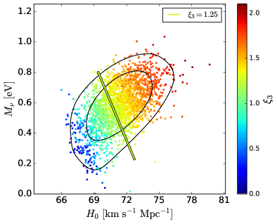
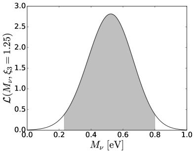
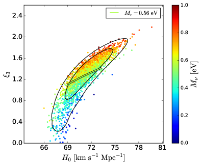
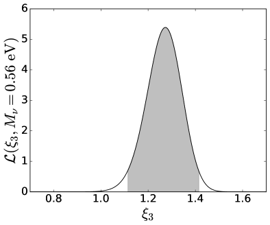
Figure 6: Left panels are the same as Figure 3 in the main text, but with the the yellow lines constrained by BAO data. The right panels show the corresponding normalized likelihood $\mathcal{L}$, with the shaded areas representing 95% CL.

Then, we can compute the likelihood function

$$\mathcal{L}\sim e^{-\chi^{2}/2},$$ (26)

based on BAO observations and determine the 2$\sigma$ range of $\mathcal{L}$, as shown in the left two panels in Figure 6. The results for ($M_{\nu}$,$H_{0}$) and ($\xi_{3}$,$H_{0}$) are shown in the upper and lower right panels of Figure 6, respectively. This estimation roughly aligns with the 95% contours in the MCMC results.