CCC++: Optimized Color Classified Colorization with Segment Anything Model (SAM) Empowered Object Selective Color Harmonization

Abstract

Automatic colorization of gray images having objects of different colors and different sizes is a difficult task. Both inter-object color variation and intra-object color variation are often seen. In addition, the main objects hold a very small area in proportion to the total image due to the large background. In the learning process, features of main objects are dominated by background features as the background components are dominant in images. As a result, a biased model is developed in favour of dominant features, and colors of main objects blend with the background colors in the resultant image. This feature imbalance problem can be solved by using weighted function for imposing higher weight to minority features as solving the class imbalance problem. With the aim of addressing this, we formulate the colorization problem into a multinomial classification problem and then apply weighted function to classes. In this paper, we propose a set of formulas to transform color values into color classes and vice versa. Class optimization and balancing feature distribution are the keys for good performance. Class levels and feature distribution are fully data-driven. We experiment on different bin size for color class transformation. Observing class appearance, standard deviation, and model parameter on a variety of extremely large-scale real-time images in practice we propose 532 color classes for our classification task. During training, we propose a class-weighted function based on true class appearance in each batch to ensure proper saturation of individual objects. We adjust the weights of the major classes, which are more frequently observed, by lowering them, while escalating the weights of the minor classes, which are less commonly observed. This adjustment aims to ensure orthodox class prediction by eliminating the domination of major classes over minor ones. In our class re-weight formula, we propose a hyper-parameter for finding the optimal trade-off between the major and minor appeared classes. This hyper-parameter testing prevent minor classes domination over the major while prioritizing the minor classes. As we apply regularization to enhance the stability of the minor class, occasional minor noise may appear at the object’s edges. We propose a novel object-selective color harmonization method empowered by the Segment Anything Model (SAM) to refine and enhance these edges. We propose two new color image evaluation metrics, the Color Class Activation Ratio (CCAR), and the True Activation Ratio (TAR), to quantify the richness of color components. We compare our proposed model with state-of-the-art models using six different dataset: Place, ADE, Celeba, COCO, Oxford 102 Flower, and ImageNet, in qualitative and quantitative approaches. The experimental results show that our proposed model outstrips other models in visualization, CNR and in our proposed CCAR and TAR measurement criteria while maintaining satisfactory performance in regression (MSE, PSNR), similarity (SSIM, LPIPS, UIUI), and generative criteria (FID).

Gray

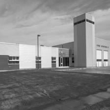
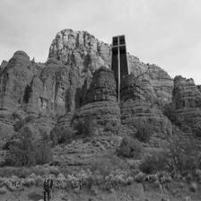
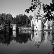
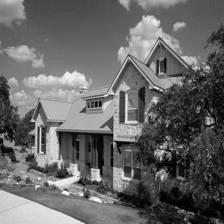
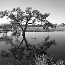
Colored

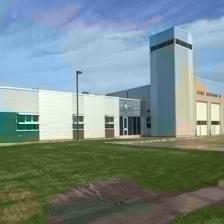
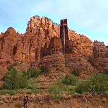
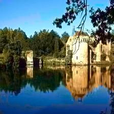
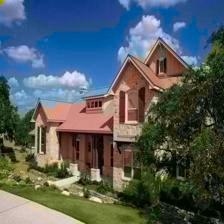
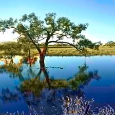
Original

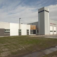
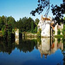
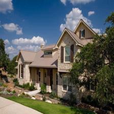
Figure 1: A visual triad illustrating the transformative power of our model and its fidelity compared to ground truth references. Grayscale inputs on the left, CCC++ colorized outputs in the center, and ground truth images on the right.

I Introduction

Human vision can perceive thousands of colors. Color is a powerful descriptor that often facilitates object identification from an image. Visual analysis of complex multispectral images is easier in color images than in grayscale images. People are still captivated by coloring, whether as a way to revive distant memories or as a means of expressing creative ingenuity. Bringing black and white material into color has a distinctive and profoundly gratifying effect. Moreover, images from antiquity, medicine, industry and astronomy are dull and unable to convey their meanings and expressions accurately. To better comprehend the image’s meaning, it is essential to colorize it. Color-coded subject continues to pique the interest of the general public, as seen by the remastered versions of vintage black and white movies, the enduring appeal of colored books for all ages, and the unexpected excitement for a variety of online automatic colorization bots. Colorization is the process of assigning color components to intensities of a grayscale image. This process is non-linear and ill-posed. A single gray image can be of many colors. For example, the color of a fruit can be light green, yellow and red. A non-living object can also hold different colors. For example, a vehicle company lunch different colors of a fixed model. During prediction, if the model predicts the red color of a car but the ground truth color of it is black then we cannot say that the prediction is wrong because the red version is also available. The natural colorization means predicting credible color distribution than the ground truth distribution. For this reason, the colorization process is not just predicting the color values of intensities of a gray image like its ground truth image color values.

Gray

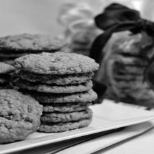
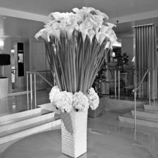
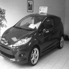
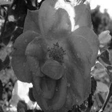
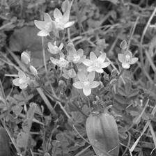
Regression

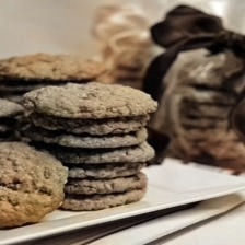
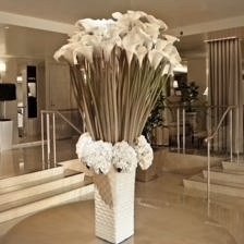
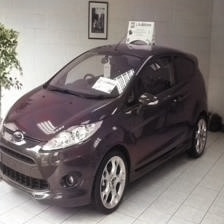
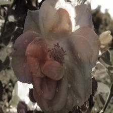
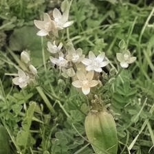
Classification

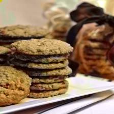
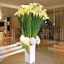
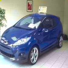
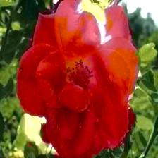
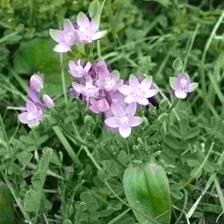
Original

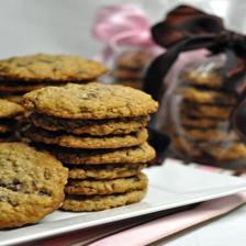
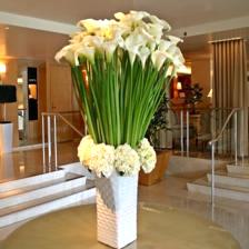
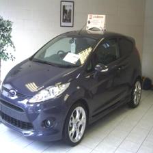
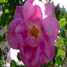
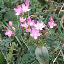
Figure 2: Results with regression and classification

Researchers employed a variety of methods for image coloring. User-guided colorization[1, 2, 3, 4, 5, 6, 7, 8, 9, 10, 11, 12] and learning-based colorization[13, 14, 15, 16, 17, 18, 19, 20, 21, 22, 23, 24, 25, 26] are the two primary groups into which existing techniques for coloring grayscale images can be categorized. Too much human interaction is required for traditional user-guided colorization to effectively colorize an image. Scribble-based colorization and example-based colorization are two sub-parts of user-guided colorization. The user-guided approach has lost favor in respect of learning-based strategies, which are easier to implement and require less human labor. A learning-based colorization approach is carried out with classical regression, object segmentation, generative approach, and classification-based techniques. Nowadays learning approaches, especially deep learning approaches are gaining in popularity for image colorization.

Deep Neural Networks (DNNs) derive representative features and hidden structural knowledge from data through multiple underlying network layers via training. Every epoch in training phase, the loss function generates feedback to refine the model’s parameters. The loss function quantifies the difference between the predicted output and the actual output, also known as the error. In every epoch, networks adjust the model’s weights proportionally to the error. The backpropagation algorithm assigns equal weight to misclassification errors of data instances belonging to each class. For imbalanced class distributions, the training procedure modifies the classifier in favor of the majority class[27]. In an unbalanced distribution, difficult instances from classes with fewer observations result in class probabilities that are lower, as predicted by the models. Incorrect and out-of-distribution instances have lower SoftMax probabilities than correct instances[28]. Since the training process with an imbalanced class distribution typically underestimates the class probability of minority class instances, learning models incorrectly classify minority class observations as hard instances[29]. Thus, the training process with an imbalanced class distribution does not hinder the model’s performance on tasks requiring unambiguous class separation, however it does impact the performance of instances that are inherently more challenging to classify. Therefore, predicted class probabilities are subsequently unreliable in imbalanced class distributions.

In the colorization problem, feature distributions are more important than class distributions. When feature distributions exhibit imbalance, similar imbalanced learning scenarios are encountered during the training process. We observed that desaturated color components are far more prevalent than saturated color components in training images. The training process is therefore biased towards the desaturated color components. It negatively affects the performance of saturated color components, causing the targeted image’s saturated color components to be biased toward desaturated color components. The training process is therefore biased towards the larger feature subsets. Therefore, the characteristics of the smaller feature subsets are eliminated by the predicted models. Occasionally, the hues of smaller objects in the image of interest merge with the background. Handling feature imbalance is of utmost significance because the smaller subsets of features are the features of interest for the learning task.

Gray

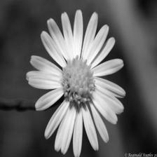
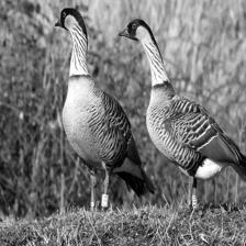
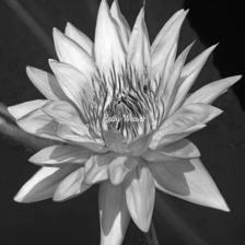
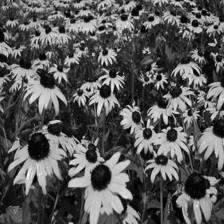
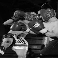
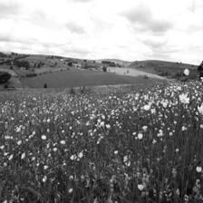
Full Class

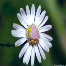
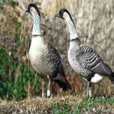
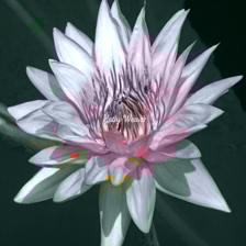
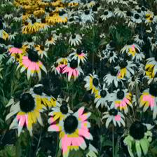
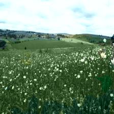
Optimized Class

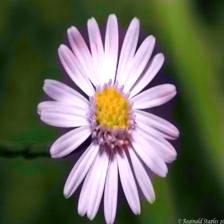
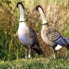
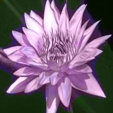
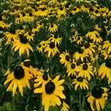
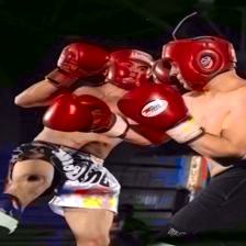
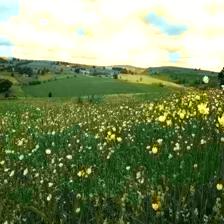
Original

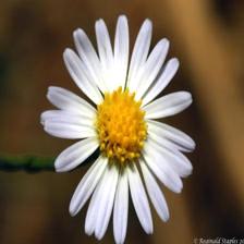
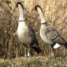
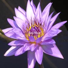
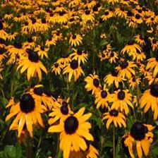
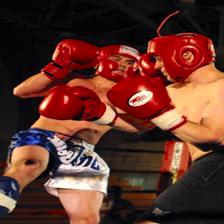
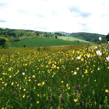
Figure 3: Results with Complete and Optimized bin

Typically, the class imbalance is addressed by resampling the dataset to achieve class parity or rescaling the data samples or employing a weighted function to impose a higher weight on the minority class [27]. In the training process, a sample’s features determine the gradient directions on the loss function. An image is comprised of pieces of varying sizes and hues. However, each unit has the same significance. The input dimension of a learning model is determined by the sample’s spatial resolution. The output dimension of colorization models is the same as the input dimension. Still there is no way to resize or reproduce a feature. Defining a set of rules that can transform feature values into class values is a solution to feature imbalance problems.

As a solution to the problems, we take motivation from the work CIC[30]. we define a set of rules to transform continuous color values into discrete color classes and vice versa to predict a distribution of possible colors for each pixel instead of the average pixel. We first transform double-channel a*b* color components to a single channel 1296 color classes, where a* channel and b* channel value range are physiclly in $[-108,108)$. In the early version of our work[31] we formed 400 classes taking bin size value as 10 and then optimized to 215 classes based on real time appearence. In this work, we experiment on different bin size and find 6 as optimal for our colorization task. All color classes are not found in real-time color images. We analyse the Place365 Validation dataset[32] and found that 532 out of 1296 color classes are mostly exist. Because redundant classes reduces classification accuracy. We apply weighted cross-entropy loss instead of classical cross-entropy loss. In this paper, we propose a technique for feature balancing. Class weights are determined by analyzing the true class of each batch during training. Rare-appeared classes need high weights than the most appeared classes to remove desaturation and biases toward major features. We re-weighted the classes making a suitable trade-off between major classes and minor classes to remove both desaturation and over-saturation. Moreover, we introduce an innovative color harmonization approach empowered by SAM (Segment Anything Model)[53]. This harmonization method is specifically designed for object-selective refinement and enhancement of color representation in images. We propose two new color image asses metrics along with previous metric of our earliest version. The basic works which are improvement of CCC++ over the work CIC[30] are illustrated in Tab. I:

TABLE I: Major differences between the CIC[30] and our proposed CCC++

Contents	CIC[30]	CCC++
Formula for color class conversion and vice versa	No	Yes
Perfect bin size approximation through experiment	No	Yes
Data driven class points optimization	No	Yes
Task generalization(Adaptibility on
similar feature imbalance problem)	No	Yes
Data driven class weight formulation	No	Yes
Hyperparameter tuning for perfect trade-off	No	Yes
Segmentation based edge refinement	No	Yes
Chromatic number ratio evaluation metric	No	Yes
Color class activation ratio evaluation metric	No	Yes
True activation ratio evaluation metric	No	Yes

The following are the contributions to this work:

1. We propose a set of formulas to transform continuous double-channel color values into discrete single-channel color classes and vice versa. Any feature imbalance regression problem can be configured to a classification job using these baseline formulas.

2. We experiment on different bin size for color class transformation. Observing class appearance, standard deviation, and model parameter on a variety of extremely large-scale real-time images in practice, we propose bin size 6 for our colorization task.

3. We optimize class levels analyzing different numerous images and propose 532 color classes for the colorization task.

4. We propose a class re-weight formula for graving high gradient from misclassified low appeared or rare classes to ensure a balance contribution of all classes in the loss. This removes feature biases as well as desaturation along with over-saturation from the color distribution and ensures orthodox prediction.

5. In our class re-weight formula we propose a hyper-parameter for finding the optimal trade-off between the major and minor appeared classes. This hyper-parameter testing prevent minor classes domination over the major classes, while prioritizing the minor classes.

6. We propose a novel object-selective color harmonization method empowered by the Segment Anything Model (SAM) to make the edge more refined and polished.

7. We propose two new color image evaluation metrics, the Color Class Activation Ratio (CCAR), and the True Activation Ratio (TAR), which quantifies the richness of color classes in generated images compared to ground truth images, providing a comprehensive measure of the color spectrum.

8. We present an abundance of quantitative and qualitative results demonstrating that our method significantly outperforms extant state-of-the-art baselines and produces reasonable results.

The rest of the paper is structured as follows. Section II is a review of the relevant literature regarding image colorization. In Section III, the entire methodology, including problem formulation and solution approach, is presented. In Section IV, we present the experimental outcomes and a comparative analysis with other cutting-edge techniques. In Section V, the conclusion is presented.

Gray

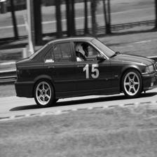
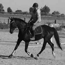
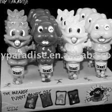
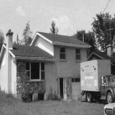
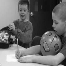
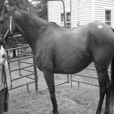
Nobalance

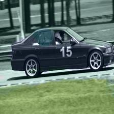
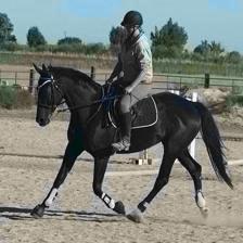
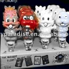
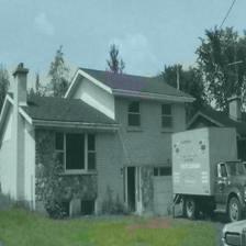
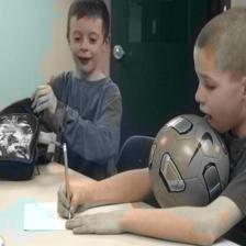
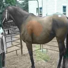
Rebalance

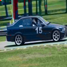
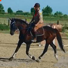
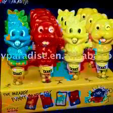
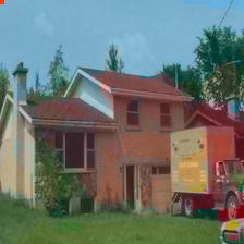
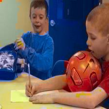
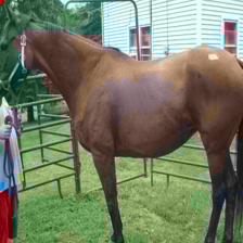
Original

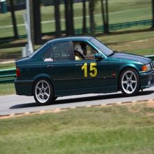
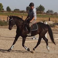
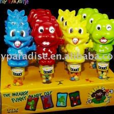
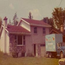
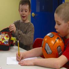
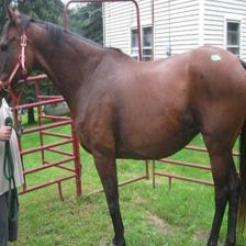
Figure 4: Results with rebalance and without rebalance

II Literature Review

II-A Background

This section will describe various colorization methodologies and the concept of how colorization methods function. It has a long history of research and is a prominent issue in computer graphics. Early approaches to image colorization relied on hand-crafted rules and heuristics, and it is referred to as user-guided colorization. In general, scribbles and examples-based coloring fall into two distinct user-interacted categories. It is unrealistic to assume that one or more reference images will provide sufficient color information to produce adequate colorization results. These approaches often lacked the ability to generate realistic outcomes. Colorization is now performed using techniques based on deep learning. Due to the fact that data-driven learning-based techniques function without human intervention, a large number of source images can be used to train the models. In terms of colorization, this refers to the automatic identification of colors that correspond well with real-world objects. Increasing the number of training samples and network layers (some cases) contributes to enhanced results. Learning-based colorization can be broadly categorized into four groups: CNN-based regression approach, object segmentation approach, generative approach, and expert system classification approach. This section provides a concise explanation of these methods.

II-A1 User Guided Colorization

Scribble Based Colorization

The scribble-based method is considered one of the most ancient techniques for colorization. The software utilizes color interpolation technique to accurately fill in missing or incomplete sections of an image, based on the user’s input in the form of scribbles.
Levin et. al.[2] proposed a technique based on optimization for propagating user-specific color scribbles to all pixels within an image. As indicated by the user’s color scribbles, adjacent pixels with identical intensity levels were designated the same color. For this endeavor, the quadratic cost function was utilized. Huang et. al.[1] proposed a method that combines non-iterative techniques with adaptive edge extraction to reduce the computational time necessary for colorization optimization and mitigate color leakage effects. Yatziv et. al.[3] introduced the concept of color blending, in which the chromatic value of a pixel is determined by the contribution of specified colors. Qu et. al.[4] proposed a technique for propagating color effectively in both pattern-continuous and intensity-continuous regions. To improve the visual impact of sparsely distributed user strokes, Luan et. al.[5] suggested incorporating nearby pixels with similar intensity and distant pixels with similar characteristics. In pursuance of the same objective, Xu et. al.[33] utilized a probability distribution to determine the most trustworthy stroke color for each pixel. Zhang et. al.[34] incorporated the U-Net structure into their colorization framework to enhance the visual effect of colorization while minimizing user interactions.

Example Based Colorization

These methods provide a more user-friendly approach to minimizing user effort by providing a reference image that is closely related to the input grayscale. Similar to the approach demonstrated by Reinhard et. al.[35], the initial study conducted by Welsh et. al.[6] involved the transmission of colors using global color statistics. Due to its disregard for spatial pixel data, the methods frequently produced unsatisfactory results in a number of instances. Various correspondence techniques have been investigated in order to obtain a more precise local transfer. These techniques include segmented region-level approaches proposed by Irony et. al. [7], Tai et. al.[8], and Charpiat et. al.[36], super-pixel level methods proposed by Gupta et. al.[37] and Chia et. al.[9], and pixel-level methods proposed by Liu et. al.[10] and Bugeau et. al. [38]. However, the process of identifying low-level feature correspondences using manually devised similarity metrics, such as SIFT and Gabor wavelet, can be prone to error in scenarios with substantial variation in intensity and content. According to Sousa et. al.[11], the color ascribed to each pixel in a grayscale image is determined by its intensity in a similarly themed reference color image. The research carried out by He et al.[12] has used deep features derived from a pre-trained VGG-19 network to achieve precise matching between visually dissimilar pictures that have semantic similarity. They used the approach of style transfer and color transfer, respectively.

Gray

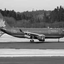
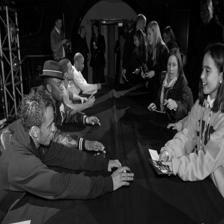
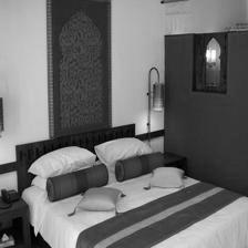
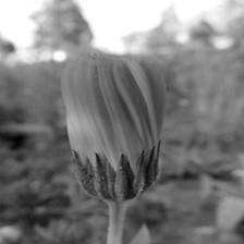
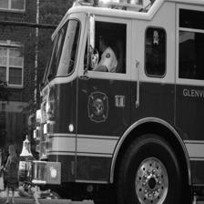
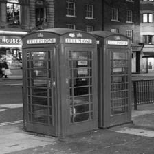
Our

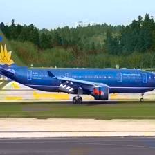
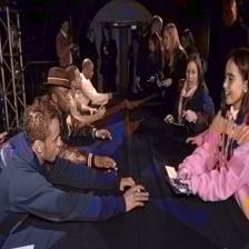
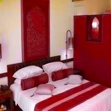
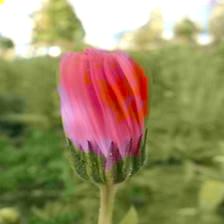
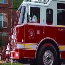
SOTA

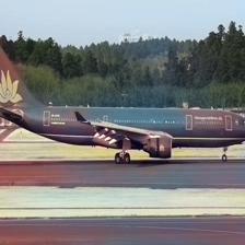
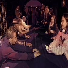
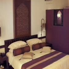
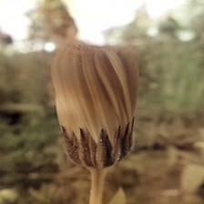
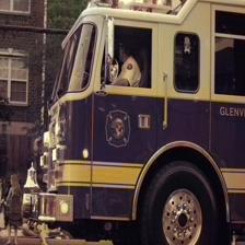
Original

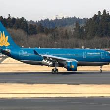
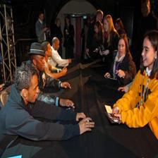
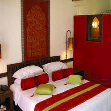
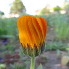
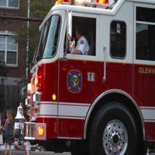
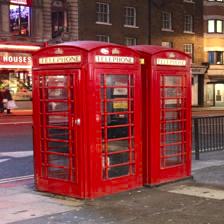
Figure 5: (A) Results of our proposed method with respect to State of The Art(SOTA) rebalance method

II-A2 Learning Based Colorization

Learning-based colorization is the process of automatic applying color to grayscale or black-and-white photographs using deep learning techniques. Learning-based colorization models directly learn the colorization process from data instead of relying on heuristics or manually constructed rules. CNNs, a subset of deep learning models, are a popular technique for learning-based colorization. The input is a grayscale or black-and-white image while the output is a corresponding color image. The CNN is trained on a large dataset of colored images. The model acquires the capacity to convert grayscale values into corresponding color values. The CNN teaches itself to comprehend the underlying relationships between gray intencity values and color values by optimizing a loss function that measures the difference between the predicted color and the actual color. This method enables the model to learn how to colorize photographs and how to apply this knowledge to new images. Basic regression-based, object segmentation-based and Generative adversarial network GAN-based are roughly three methodologies in learning-based colorization. The major issue regarding colorization using machine learning techniques is feature balancing for focused objects and background of the images. A few research have been done on this issue for machine learning techniques.

Basic Regression Based Colorization

For colorization, conventional CNN or specialized architectures such as InceptionNet, VGGNet, ResNet, DenseNet, etc. are utilized. Grayscale images are fed to the network as input and color channels are estimated. The MSE, MAE, RMSE, etc. are then employed to calculate the loss between estimated color channels and true color channels. An optimizer is utilized to minimize loss and achieves ideal color distribution. Using four pre-trained VGG16[39] layers, Dahl et al.[40] developed an automated method for generating full-color channels from gray images. The design and construction of an automated grayscale image colorization system by Hwang et. al.[41] was based on the baseline regression model. Baldassarre et al.[42] proposed a technique that incorporates Deep CNN and Inception-ResNet-v2 [20]. Using this pre-trained Inception-ResNet-v2 model, feature extraction at a high level is achieved. Moreover, the network is trained from scratch. Iizuka et al.[24] developed an end-to-end method that simultaneously learns global and local image attributes. This method employs categorization labels (photo categories) to enhance model performance.

Encoder-decoder based colorization model proposed by Nguyen-Quynh et. al.[43] using both global and local priors. Encoder-decoder CNN architecture with filtering-based rebalancing methods was presented by Gain et. al.[21] in order to colorize photographs. Yun et. al.[44] propose a novel point-interactive colorization Vision Transformer (iColoriT) that utilizes the global receptive field of Transformers to distribute user stimuli to appropriate locations. Using the Transformers’ self-attention mechanism, iColoriT can selectively colorize important regions using only a few local signals.

Object Segmentation Based Colorization

Objects within an image are segmented, and the network then takes these segments as input along with the full images. The network can learn color assignment segment-wise or object-wise. After an image has been segmented, the colorization model assigns colors to its segments using a variety of techniques. To select the correct colors, the model may, for example, consider the degree to which the reference image and the grayscale image share color similarities. Alternately, the model may employ additional data, such as spatial connections between segments or global color coherence, to generate colorization results that are more consistent and aesthetically appealing. Su et. al.’s[25] instance colorization network relied on the extraction of both full-image and object-level colorization information. Xu et al. [28] proposed a paradigm for the automated colorization of images based on the technology of semantic segmentation. They utilized a network for semantic segmentation to accelerate the convergence edges of the image. Hesham et al.[45] proposed a scaled-YOLOv4 detector-based colorization model. They utilized coloration to distinguish various objects in multi-object images. Kong et al.[46] presented an adversarial edge-aware model for image colorization that integrates multitask output and semantic segmentation. To extract rich semantic properties from a given grayscale, they employed a generator that learns colorization from chromatic ground truth values. Using only point annotations and a convolutional neural network (CNN), Xia et al.[47] created a method for segmenting nuclei that are inadequately supervised. The suggested method effectively combines a secondary colorization task with an inadequately guided segmentation task.

Gray

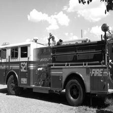
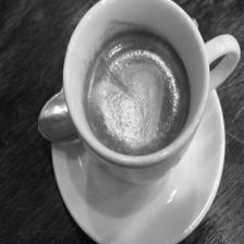
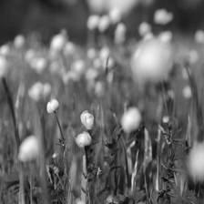
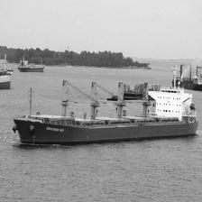
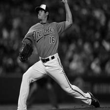
Our

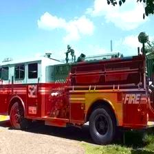
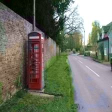
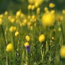
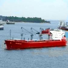
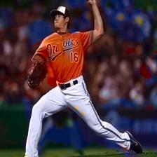
SOTA

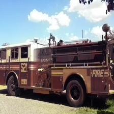
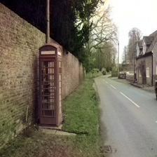
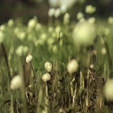
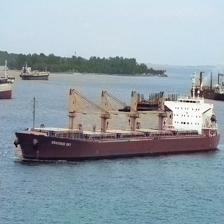
Original

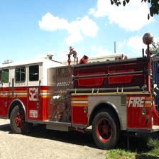
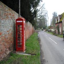
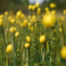
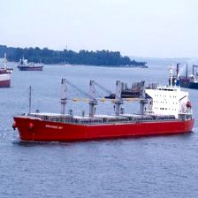
Figure 6: (B) Results of our proposed method with respect to State of The Art(SOTA) rebalance method

GAN Based Colorization

GAN (Generative Adversarial Network) based image colorization models combine discriminator and generator networks to produce realistic and aesthetically pleasing colorized photographs. These deep learning models are comprised of two fundamental components: a generator network that creates colorized images from grayscale or black-and-white images, and a discriminator network that distinguishes between actual and created images. The discriminator network determines if colored images are genuine or fake and provides input to the generator network in order to generate more visually comparable colorized images. Through competition between the generator and discriminator networks, the model is able to learn the underlying patterns and color distributions from the training dataset and an improved colorization result is obtained. Wu et al.[13] proposed a generative adversarial network-based approach for image colorization that uses semantic information at a fine granularity level. They created a collection of ethnic costumes that represent four subgroups of Chinese minorities using a Pix2PixHD-based coloring model. Guo et al.[16] proposed a GAN-based, bilateral Res-U-net model for image colorization. Ozbulak et al.[48] employed Capsule Network (CapsNet) for image colorization. The original CapsNet’s generative and segmentation capabilities were recommended for the classification of images, but the network was modified and used to colorize the images instead. Wu et al.[14] proposed a GAN-based model. Generative adversarial networks with enhanced and diversified color priors were used to retrieve dazzling colors. Using a GAN encoder, they identified matching features that were comparable to exemplars and then modulated these features into the colorization procedure. Bahng et. al.[17] proposed a model consisting of two conditional generative adversarial networks. The first network converts text to a palette, whereas the second network uses the palettes to colorize images. To protect colorized medical images and improve the quality of synthetic images, Liang et al.[18] introduced a colorization network based on the cycle generative adversarial network (CycleGAN) model that incorporates a perceptual loss function and a total variation (TV) loss function. Treneska et al.[49] proposed a method that generates color images using generative adversarial networks (GAN). Transfer learning was also applied to visual comprehension. Wu et al.[15] introduced a novel technique for coloring remote sensing images utilizing deep convolution GAN. The GAN generator accumulates visual characteristics. The generator and discriminator effectively collaborate to produce color images. For the purpose of colorizing images, Zang et al.[19] developed the bi-stream generative adversarial network colorization model (BS-GAN). The BS-GAN generator is capable of acquiring both global and local properties by fusing two parallel streams.

Feature Balancing for Colorization

Zhang et al.[30] proposed an automatic colorization method (CIC) using CNN. The model learns to classify intensity into predetermined color level and then assigns corresponding color based on classified class level. Zhang’s approach defines 313 classes. During training, they utilized class rebalancing to broaden the color palette of the output image for solving feature imbalance problem. An et al.[23] used a VGG-16 CNN model based classification model for colorization. They set 313 classes as in Zhang et al. method. The method also utilized a color rebalancing technique to solve feature imbalance problem. Gustav et al. [20] used the unbalanced loss of classification for solving feature imbalance. Their model predicts hue and chroma distributions for each pixel intensity. Gain et. al.[22] proposed a deep localized network which is a new model for image colorization. Instead of employing the global loss, they utilized the color-specific local loss to solve feature imbalance issue. These methods are promising for colorization problems. However, some methods show good performance on typical scenes (e.g. landscapes, sky, ground, etc.), but still their success is limited on complex images with foreground objects.

II-B Related Work

DeOldify[50] is a deep learning-based picture and video colorization model that incorporates strategies from generative adversarial networks (GANs) with self-attention processes. DeOldify uses its GAN architecture and self-attention techniques to produce accurate and aesthetically pleasing colorizations after being trained on a large dataset of colored and grayscale photos. DeOldify has grown to be a well-liked application for adding color to black-and-white images, including historical photos and movies, with excellent colorization outcomes and an approachable interface. It offers options for user instruction and transfer learning from ImageNet.

Ijuka et. al.[24] introduced a deep learning framework that combines global and local networks to perform image colorization with simultaneous classification. By integrating high-level global image priors and local patch-based priors, the model learns to predict colors for grayscale images based on semantic context. This joint learning approach enhances the colorization results by aligning colors with the semantic context of the images, leading to visually appealing colorizations and accurate image classification.

Larsson et al.[20] proposed a method for automatic image colorization that used convolutional neural networks (CNNs). To extract high-level features from grayscale photos and to provide appropriate colorizations, the method entailed training an encoder-decoder architecture. The model produces colors that match human perception and the produced images have a realistic appearance by optimizing with a perceptual loss function that takes perceptual similarity metrics into account.

A CNN-based automated colorization was suggested by Zhang et al.[30]. The whole color spectrum is classified into 313 groups (classes). To broaden the range of colors in the output picture, they employed class rebalancing during training. Additionally, they proposed LPIPS (local patch image patch similarity), a brand-new testing framework for colorization algorithms that may be used for various image synthesis applications.

Low-level cues and high-level semantic data were combined by Zhang et al.[34]. Their approach incorporates user input and makes use of deep priors that have been learned enabling real-time interactive image colorization. It offers a network architecture and training technique that enables users to input color hints or strokes to direct the colorization process creating aesthetically pleasing and cohesive colorized outcomes in real time.

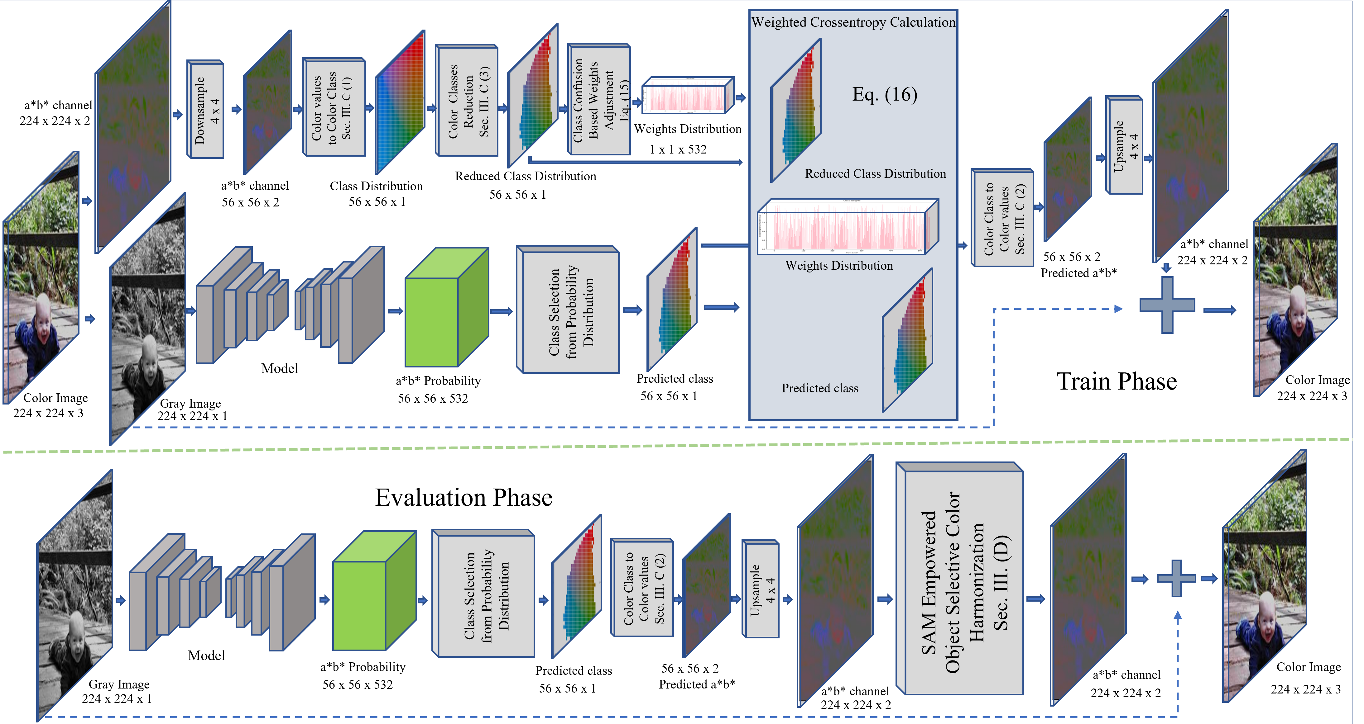
Figure 7: CCC++ with SAM empowered object selective color harmonization.

Su et al.[25] proposed a learning model that was based on the extraction of both full-image and object-level information for colorization. To create accurate and contextually consistent colorizations, the method takes into account the unique instances or objects inside a picture. Instance segmentation allows for the autonomous treatment of each item during colorization and assigns exact colors assignment depending on object properties.

Gain et al.[21] proposed an encoder-decoder CNN architecture with filtering-based rebalancing algorithms for colorizing pictures. They employ a traditional CNN for color value prediction and a dense neural network for feature extraction. To eliminate desaturation, they suggested region-based color rebalancing approaches.

Gain et al.[22] proposed a learning based model for naturalistic colorization. The feature set of examples is initially grouped into several feature subsets (similar groupings). Loss functions are computed for every subset of features instead of a single global loss function. The backpropagation algorithm was created based on local loss functions. The proposed algorithm propagates losses computed by a subset of features into the respective nodes of the hinder layers from which that subset of features is extracted, in contrast to conventional models which propagate global loss as feedback into hinder layers.

Zang et al.[19] integrated a unique texture-aware bi-stream GAN into the established encoder-decoder framework. The bi-stream feature extraction module (BSFEM) and the feature boosting module (FBM) extract the global and local features from two parallel encoders and fuse them using a novel hybrid attention structure. This novel structure could highlight the importance of specific channels and locations of features that potentially benefit image colorization process. The suggested multi-scale feature attention module (MSFAM) can also help for better recovery of the texture colors.

III Methodology

III-A Color Space

The most commonly and frequently used color space is conventional RGB, where Red, Green, and Blue are the three main colors. All conceivable combinations of the three colors are used in standard RGB. However, in RGB space, color information and content information cannot be separated. Therefore, it is not suitable for color manipulation in colorization tasks because there is a chance to change the context information during color manipulation. Therefore, common usage is CIELAB[51] color space instead of RGB. Because color information can be separated from context information in La*b* (LAB) space and color information can be manipulated while keeping context information unchanged. In La*b* space, L denotes the brightness or luminosity of the image. Intensities fall between $[0,100]$, where the value $0$ designates black and $100$ designates white. Colors get brighter as $L$ rises. The a* denotes the image’s proportion of red or green tones. The red is represented by a positive a* value and the green is represented by a significant negative a* value. The b* denotes the image’s proportion of yellow or blue tones. Yellow is represented by a high positive b* value. Blue is represented by a significant negative b* value. Although a* and b* does not have a single range, values frequently lie between $[-128,127]$.

III-B Problem Definition

The colorization problem is considered as predicting color channels from a given gray channel. The Lightness (L) channel of La*b* color space can be mapped into the gray channel (intensity) and vice versa[51]. Furthermore RGB can be mapped into LAB and vice versa. The task can be defined as follows in Eq. 1, 2, 3, and 4.

$$X_{ab}=f(X_{L})$$ (1)

$$Distance_{min}=(Y_{ab},X_{ab})$$ (2)

$$X_{Lab}=concat(X_{L},X_{ab})$$ (3)

$$X_{L}\in\mathbb{R}^{H\times W\times 1},X_{ab}\in\mathbb{R}^{H\times W\times 2},Y_{ab}\in\mathbb{R}^{H\times W\times 2}$$ (4)

where $X_{L}$ is the lightness channel, $X_{ab}$ is the predicted color channel, $X_{Lab}$ is the predicted color image, $Y_{ab}$ is the ground truth color channel, $f(.)$ is the mapping function achieved by deep learning, $Distance_{min}(.)$ is the objective function (can be any loss function) by which the optimizer makes the learning efficient, $\mathbb{R}$ is the total image component, $\mathbb{H}$ and $\mathbb{W}$ are the image dimension.

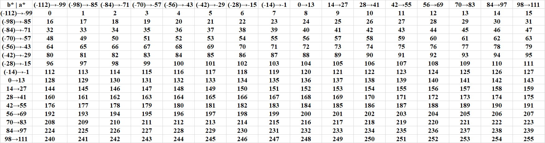
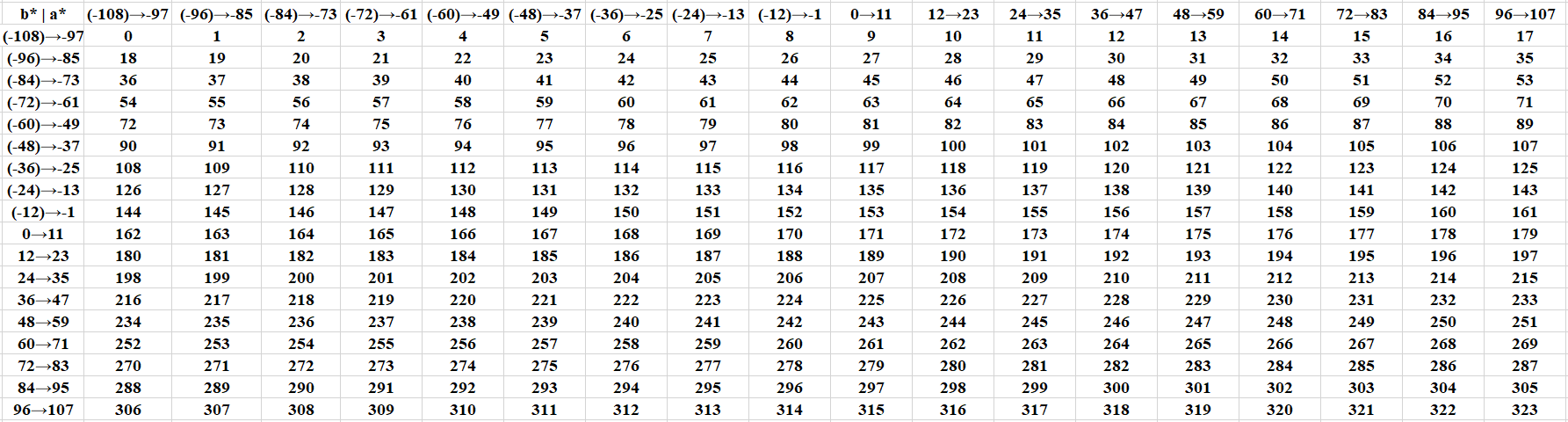
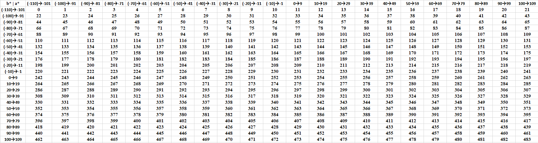
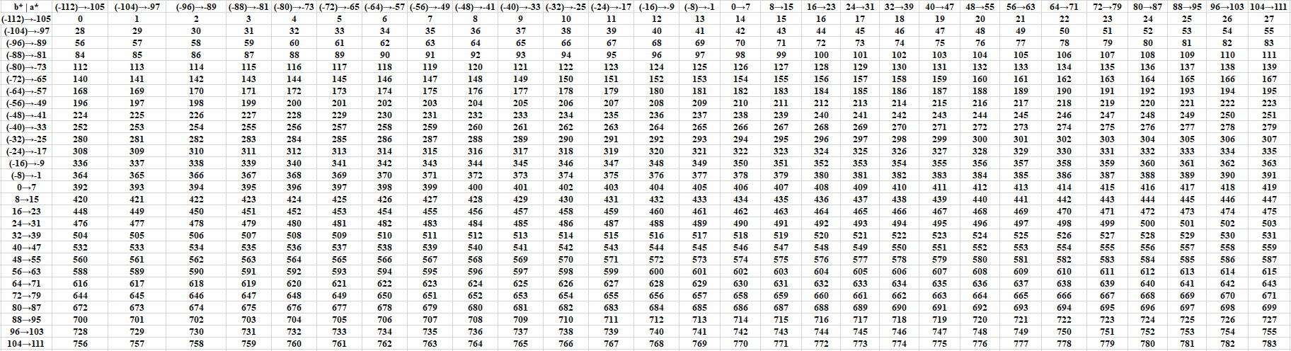
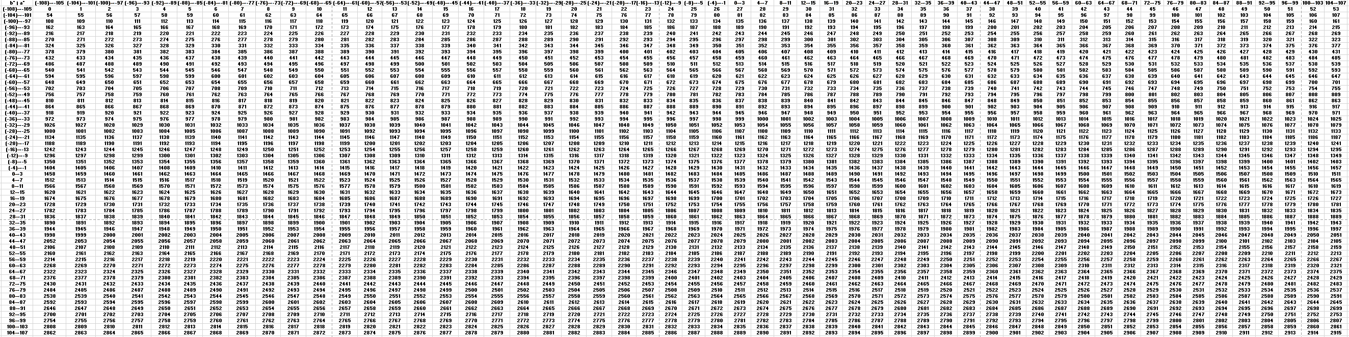
Bin Size = 14 Bin Size = 12 Bin Size = 10 Bin Size = 8 Bin Size = 6 Bin Size = 4

Figure 8: Continuous color values to discrete color classes for different bin sizes.

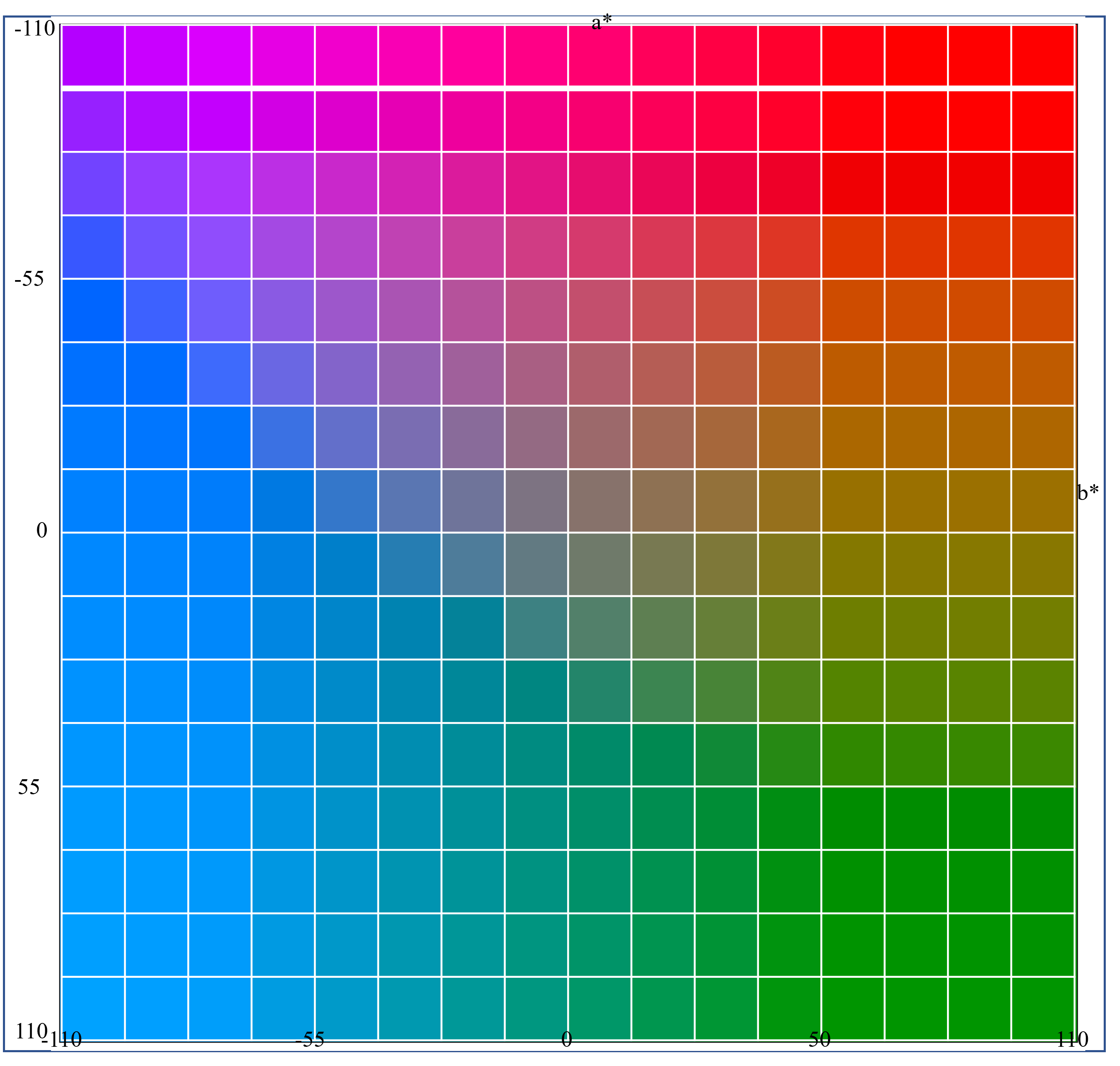
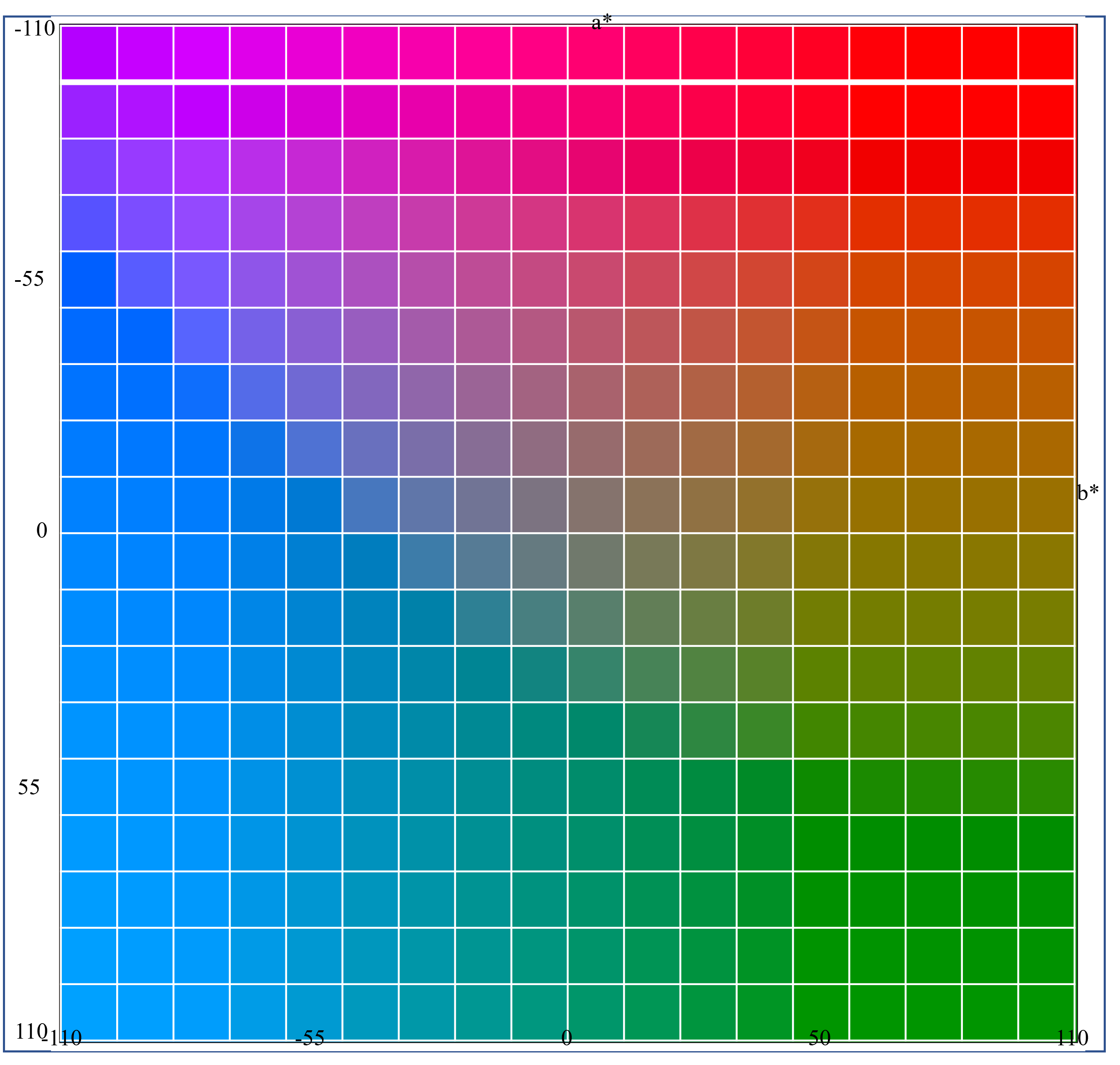
Left: bin size = 14; Right: bin size = 12
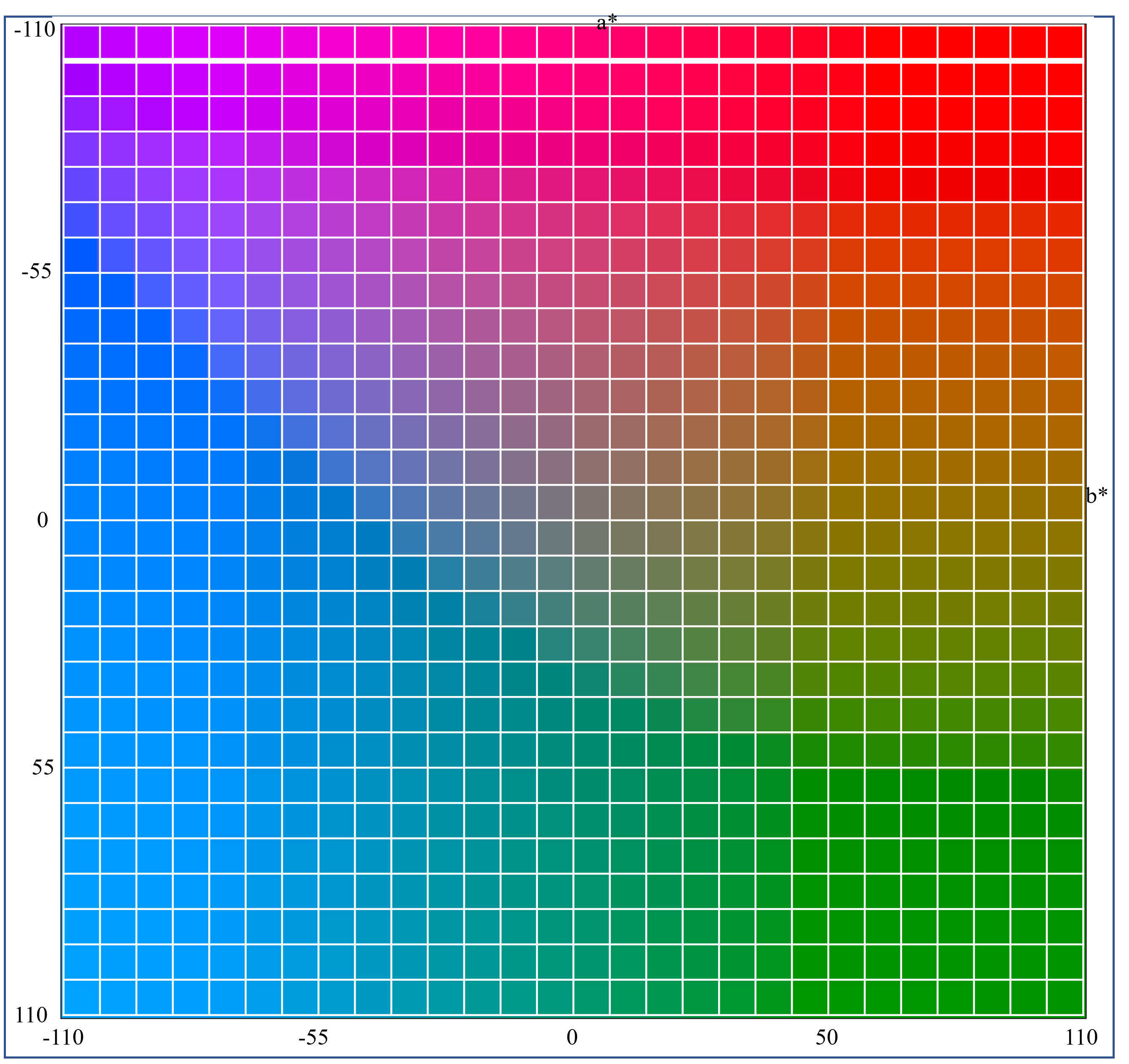
Left: bin size = 10; Right: bin size = 8
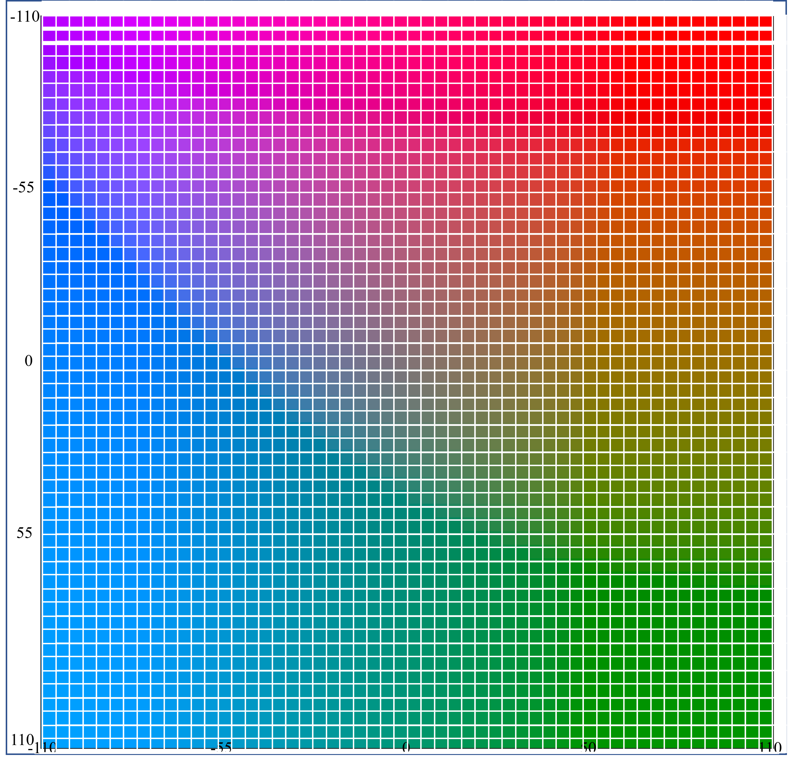
Left: bin size = 6; Right: bin size = 4

Figure 9: Color visualization of discrete color classes for different sizes.

Theoretically, the values of the a* and b* channel are continuous within [-128, 127]. So, the prediction is considered a regression problem. Therefore, the $Distance_{min}(.)$ of equation 2 naturally can be either L1 loss or L2 loss or Huber loss or Log-cosh loss or similar regression loss. Loss functions are shown below.

$$L_{1}(Y_{ab},X_{ab})=\frac{1}{N}\sum_{N}|Y_{ab}-X_{ab}|$$ (5)

$$L_{2}(Y_{ab},X_{ab})=\frac{1}{N}\sum_{N}(Y_{ab}-X_{ab})^{2}$$ (6)

$$L_{\delta}=\left\{\begin{matrix}\frac{1}{N}\sum_{N}\frac{1}{2}(Y_{ab}-X_{ab})^{2},&|Y_{ab}-X_{ab}|<\delta\\ \frac{1}{N}\sum_{N}\delta((Y_{ab}-X_{ab})-\frac{1}{2}\delta),&otherwise\end{matrix}\right.$$ (7)

$$Log-Cosh(Y_{ab},X_{ab})=\frac{1}{N}\sum_{N}log(cosh(Y_{ab}-X_{ab}))$$ (8)

where $N$ represents the total number of pixels in a batch and $\delta$ represents the acceptable threshold. Background colors such as clouds, soil, pavement, and walls cover the majority of the areas in the real-time images. The color components of the primary or focal objects are substantially smaller than the total color components. This results in an unbalanced distribution of features. Handling feature imbalance is crucial because the smaller subsets of features are the feature of interest for the learning task. The colorization problem’s inherent ambiguity and multimodality make the above loss functions vulnerable. If an object can take on a variety of a*b* values, the mean of the set is the most effective method to solve the loss shown in Eq. 5, 6, 7 and 8. The averaging error effect favors color values that are predominantly covered in the ground truth image. In an imbalanced feature distribution, the training process is therefore biased towards the larger feature subsets and colors of smaller objects evaporate from the resulting models. Therefore, the distribution of a*b* values is skewed towards desaturated values, and the color of minuscule objects disappears.

III-C Solution Approach

III-C1 Continuous Color Range to Discrete Color Classes

The a* and b* color channels are continuous within the range $[-128,127]$. Each a*b* pair with a lightness value $L$ forms a RGB color pixel. We can get a a*b* pair from a*b* color space that is a 2-D space, where a* is one direction and b* is another direction. For a fixed $L$, small change in a*b* pair has no psychovisual effect. Therefore, human perception of the information in an image normally does not involve quantitative analysis of every pixel value in the image. As we know colorization is a regression problem where the regression model predicts the continuous quantities of a* and b* for a given $L$. Taking the advantage of psychovisual nature of human, the colorization problem can be represented as a classification problem where the learning model predicts a discrete class level for a a*b* pair. To fomularize the problem, the a*b* color space is divided into bins of a fixed grid size and each bin is assigned a discrete class level. The formula is given below in Equation 9.

$$C=\frac{b^{*}+\beta}{\alpha}\times\Delta+\frac{a^{*}+\beta}{\alpha}$$ (9)

where a* and b* are the continuous color channels, $C$ is the discrete class level of color values within a bin, $\alpha^{2}$ is the area of a bin, $\beta$ is a shifting constant that shift a*b* color values into positive quadrant, $\delta$ is the number of grids in each a* or b* color channel.

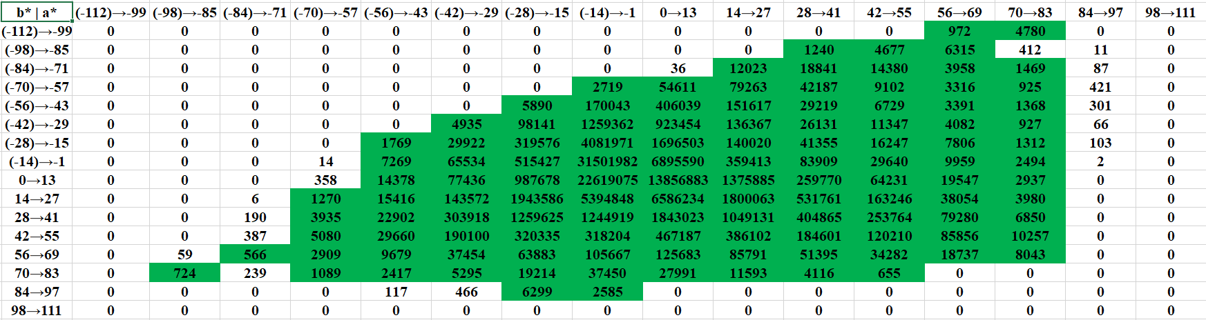
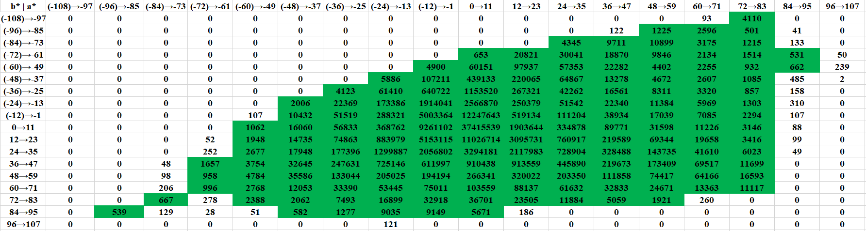
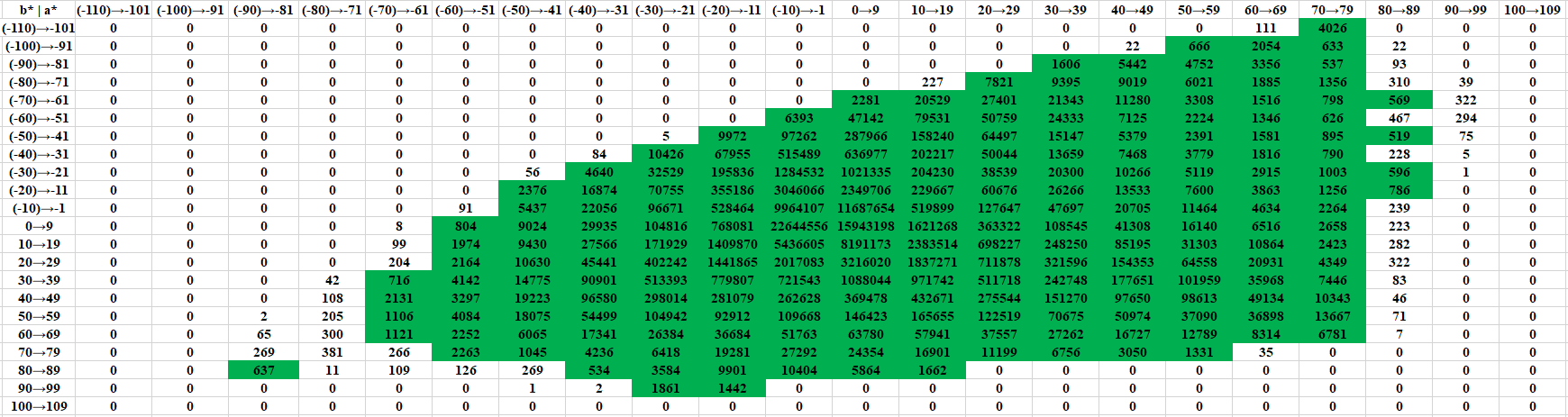
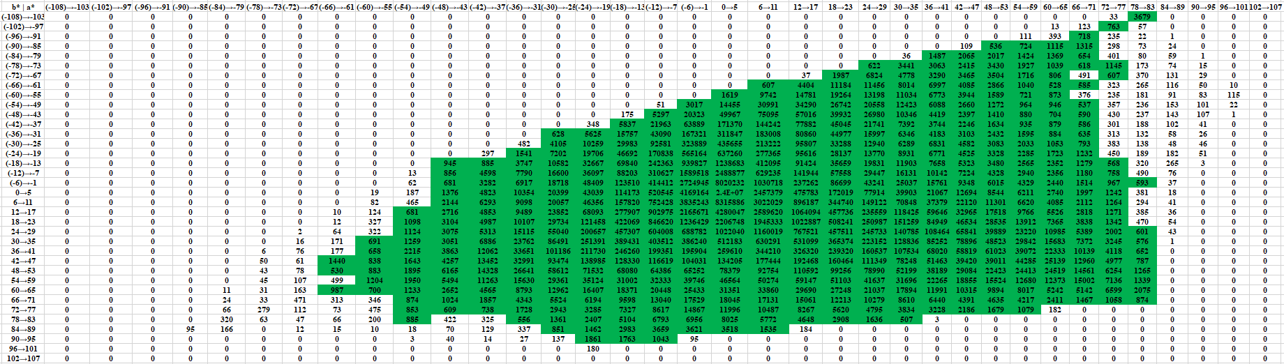
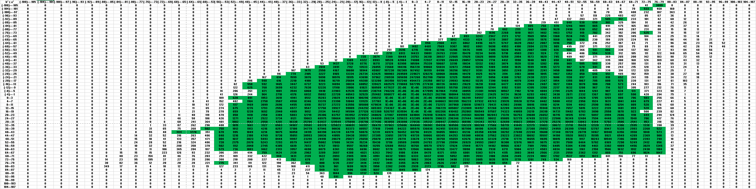
bin size = 14 bin size = 12 bin size = 10 bin size = 8 bin size = 6 bin size = 4

Figure 10: Real-time appearance of Color classes in place365 validation dataset.

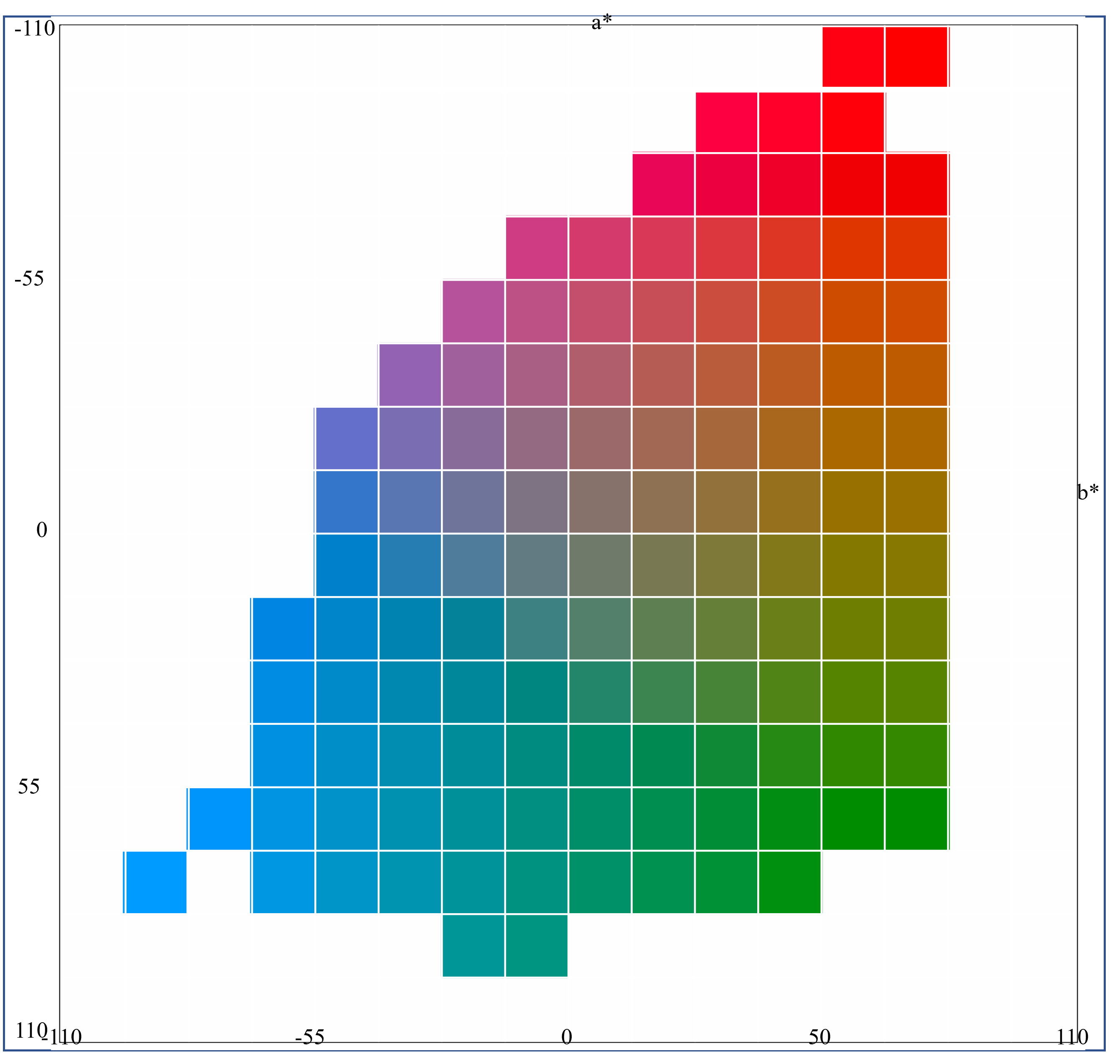
Left: bin size = 14; Right: bin size = 12
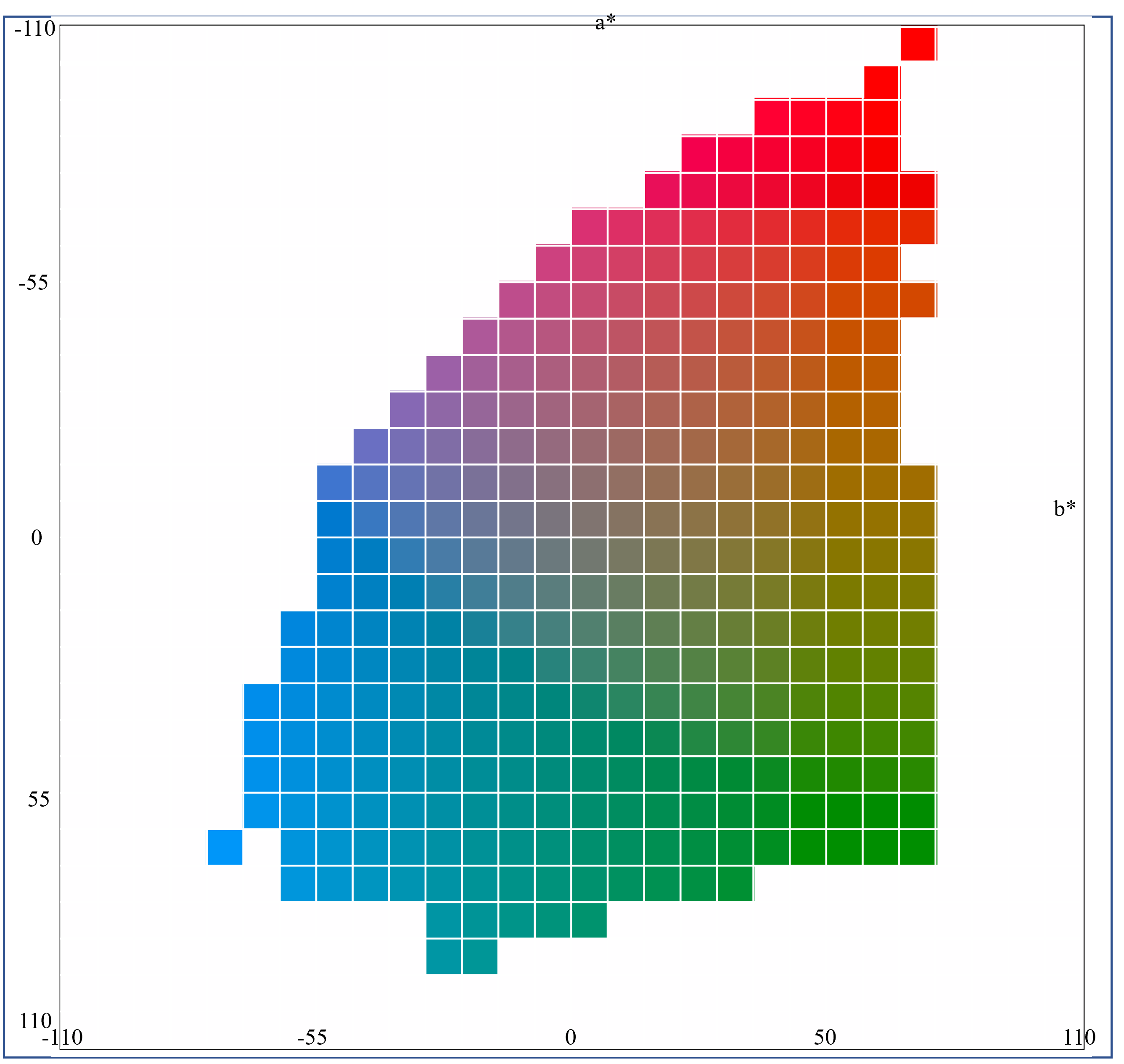
Left: bin size = 10; Right: bin size = 8
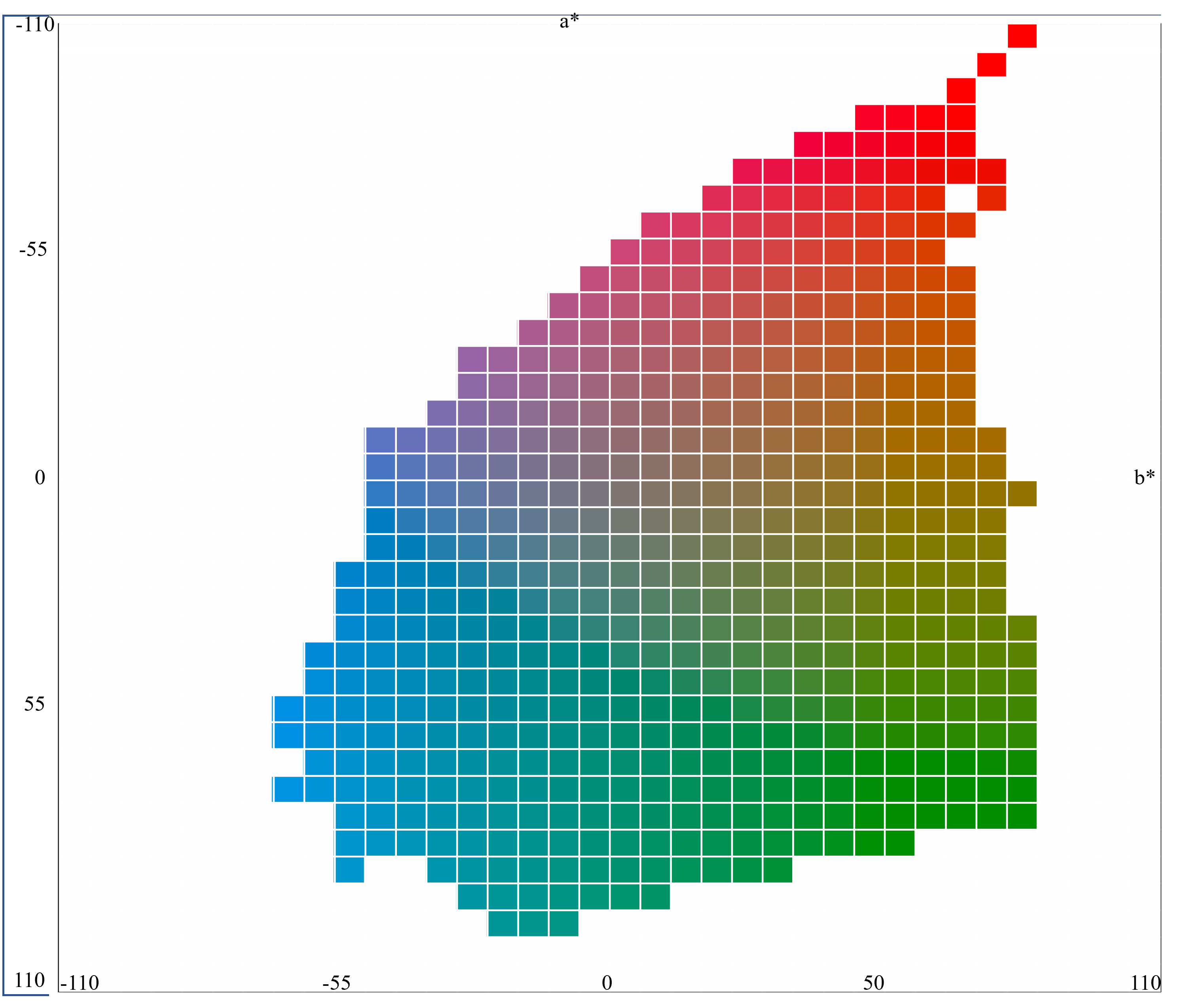
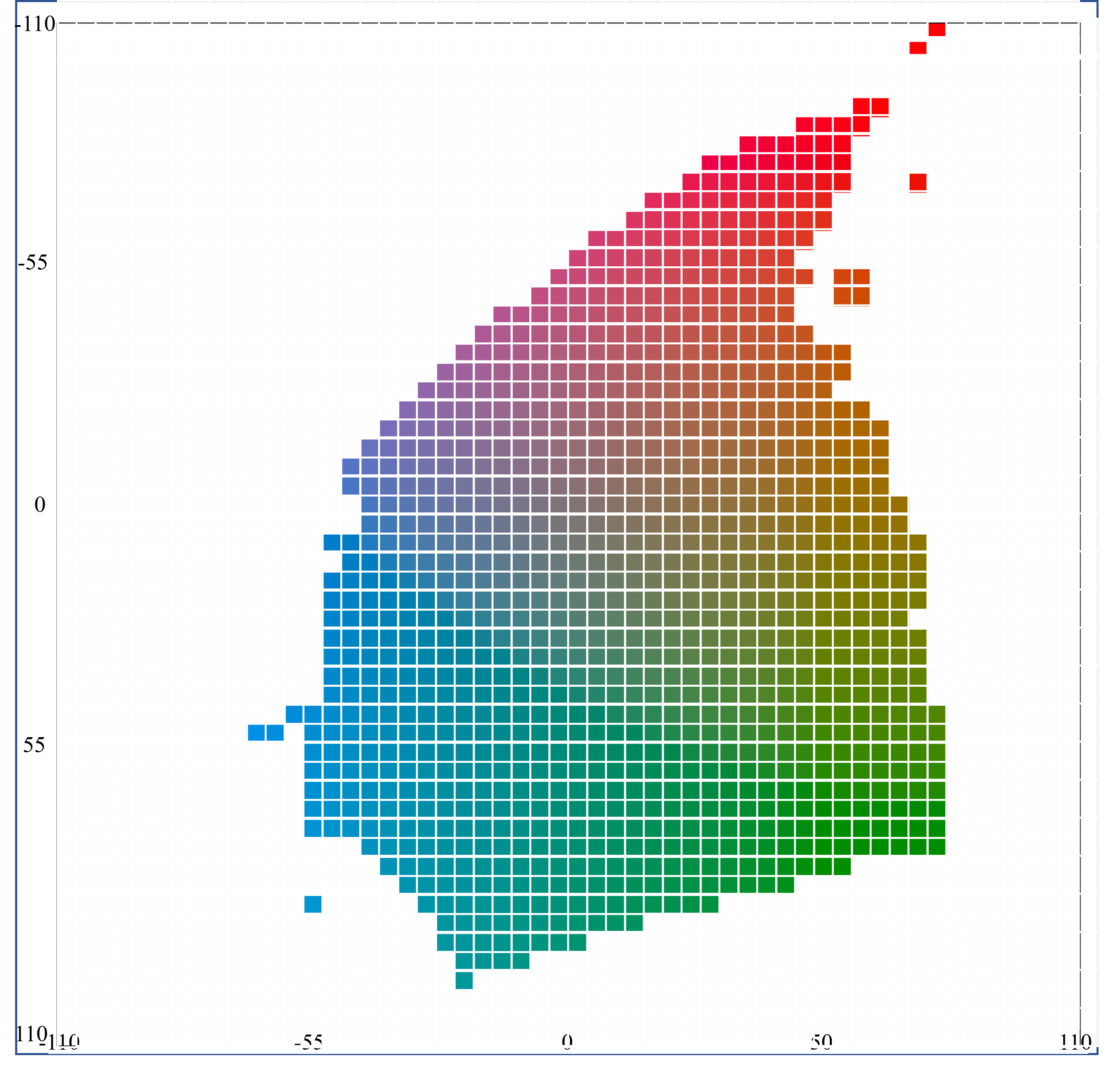
Left: bin size = 6; Right: bin size = 4

Figure 11: Visualization of real-time appearance of Color classes in place365 validation dataset.

TABLE II: Bin size approximation

	Total	Optimized	a*b*		RGB (L $\in$ 50)
Bin	Class	Class	Max.	Avg.	Maximum Deviation				Average Deviation
Size	Points	Points	Dev.	Dev.	a, b $\in$ 50	a, b $\in$ 0	a, b $\in$ -50	Avg.	a, b $\in$ 50	a, b $\in$ 0	a, b $\in$ -50	Avg.
4	2916	1049	2	1	2.39	2.43	1.9	2.24	1.59	1.60	0.71	1.30
6	1296	532	3	1.5	4.85	4.66	3.25	4.25	2.39	2.43	1.9	2.24
8	784	325	4	2	6.55	6.33	4.75	5.88	3.20	3.24	2.45	2.96
10	484	218	5	2.5	8.29	7.78	5.5	7.19	4.01	3.95	2.92	3.62
12	324	159	6	3	10.10	9.44	6.65	8.73	4.85	4.66	3.25	4.25
14	256	121	7	3.5	12.00	10.87	7.75	10.20	5.70	5.60	4	5.10

III-C2 Color Class to Visual Color Mapping

We need to extract a*b* pairs from the predicted color classes, $C$s, generated by the learning model for color image generation. Each bin is assigned by a fixed color class level $C$ which is driven by $a^{*}$ and $b^{*}$. The formulas are given below in Eq. 10, 11, which are the reverse of Eq. 9.

$$a^{*\prime}=[(C\mod\Delta)\times\alpha]-\beta+\frac{\alpha}{2}$$ (10)

$$b^{*\prime}=[(C\div\Delta)\times\alpha]-\beta+\frac{\alpha}{2}$$ (11)

According to the above equations, the maximum loss for each a* or b* value is $\frac{\alpha}{2}-1$. The higher value of $\alpha$ reduces the number of classes but makes the representation lossy as a large continuous range is converted to a single class. However, handling the problem with lower class is easy. The lower value of $\alpha$ increases the number of classes. In general, there is no guarantee that increasing or reducing the number of classes will increase classification accuracy. In colorization problem, more classes make the prediction less precise. It is important to adjust the number of class levels for a*b* color space so that modified $a^{*}b^{*}$ can describe image’s color nature.

III-C3 Color Class Reduction Based on Practical Appearance

The a* and b* color values are continuous within $[-128,127]$ in the a*b* color channel. However, in practice, the range is found within $[-100,100]$. We first transform the continuous $[-108,108)$ ranged a*b* color channel to a single plane of 1296 color classes by taking $\alpha=6$, $\beta=108$ and $\delta=36$ in Eq. 9. A 2D grid of bins as $36\times 36$ single plane array is then formed where horizontal axes indicate a* and vertical axes indicate b* color information. Each coordinate is assigned a class value. The class matrix is shown in Figure 8. The proposed color class to visual color is shown in Figure 9. From Figure 9 we see that the whole image has a smooth representation of different colors. Colors of the nearest bins or blocks are almost similar. Color changes gradually block by block. We choose bin size 6 as we find it optimal for the colorization task. High bin size generates less class points and requires less model parameter. However, it increases the maximum and average deviation from the actual pixel during color values retrieval. Low bin size decreases the deviation but generates much classes and requires much model parameter. The bin size approximation is shown in Tab. II, and relative comparison is shown in Figure 13.

With 1296 color classes we experimented with the Place365 Validation dataset [32] as a reference dataset. We see that some color classes face starvation in real-time images. The result is shown in Figure 10. In the Place365 Validation dataset, there are 36,500 images in total. We took 35040 images randomly from the dataset and extracted classes from them. We downsampled the images to $56\times 56$ to reduce the number of class samples in the training process. Therefore, there were a total of 109885440 (109.88M) class samples with 1296 class levels. Each color pixel is a color class sample with a specific color level. We calculate class level histogram on total class samples. We consider a class level for training samples if the class level has minimum of 500 (0.000455%) class samples out of 109885440 class samples. The class samples less than 500 with a specific class level is mapped to their nearest-neighbor present class levels using fixed centroid $k$-means clustering which is shown in Eq. 12. The class in the final color bin, which is shown in Figure 11. 500 pixels of a color is very minimum compared to the total pixels of 35040 images because very few images have very few number of that color and the most of the images do not contain this color. Finally we get 532 color classes within 1296 color classes which have more than 500 pixels. Class optimization is a major issue for colorization model. Less class may make the model more error-free, but it makes some color visuals outside of the bin. As one of our targets is to keep the rare appeared color values in the predicted distribution, we need to keep those rare color visuals active in the training process.

$$kmeans(C,\mu)=argmin\sum_{i=1}^{k}\sum_{C}||c-\mu_{i}||^{2}$$ (12)

where $C$ is the input color class vector, $\mu$ is the approved color classes for training, and $k$ is the number of color classes (532). We can define $\mu$ as the fixed value centroid. The iteration will happen single time and the centroid value will be unchanged.

III-C4 Network Architecture

We build our model based on an encoder-decoder architecture. For the encoder part, we use DenseNet for our feature extractor. The DenseNet is a high-level feature extractor that is suitable for good color value generation. For the decoder part, we use conventional CNN. The network architecture of our proposed method is shown in Figure 12.

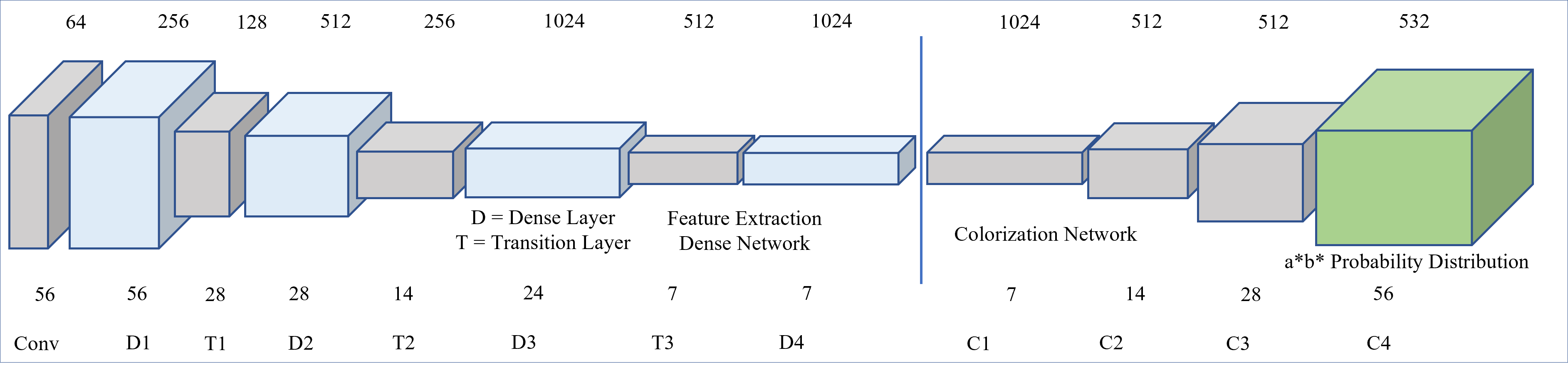
Figure 12: Network architecture of CCC++

TABLE III: The model structure of the DenseNet

Layers	Output Size	DenseNet-121		Outputs
Convolutional	$112\times 112$			64
Pooling	$56\times 56$			64
Dense Block 1	$56\times 56$	$1\times 1$ conv	$\times 6$	256
		$3\times 3$ conv
Transition 2	$56\times 56$	$1\times 1$ conv		128
	$28\times 28$	$3\times 3$ conv
Dense Block 2	$28\times 28$	$1\times 1$ conv	$\times 12$	512
		$3\times 3$ conv
Transition 2	$28\times 28$	$1\times 1$ conv		256
	$14\times 14$	$3\times 3$ conv
Dense Block 3	$14\times 14$	$1\times 1$ conv	$\times 24$	1024
		$3\times 3$ conv
Transition 3	$14\times 14$	$1\times 1$ conv		512
	$7\times 7$	$3\times 3$ conv
Dense Block 4	$7\times 7$	$1\times 1$ conv	$\times 16$	1024
		$3\times 3$ conv

• Feature Extraction: The connections between the layers of DenseNet are robust. It minimizes the gradient vanishing problem and has less semantic information loss during feature extraction than previous CNN models [52]. The output from each subsequent layer is concatenated by the DenseNet. To adapt the model to grayscale input, we change the first convolutional layer. To build a $\frac{H}{32}\times\frac{W}{32}\times 1024$ feature representation from DenseNet, the final linear layer is discarded. These characteristics are utilized as input in the CNN-based colorization network. Table III displays the various DenseNet convolutional layers and outputs.

• Colorization Network The network employs several convolutional and up-sampling layers after receiving an input of a $\frac{H}{32}\times\frac{W}{32}\times 1024$ feature representation. The fundamental nearest-neighbor method is what we employ for up-sampling. The $H\times W\times 2$ a*b* tensor is what the network outputs. In Table IV, the various convolutional layers and their results are displayed.

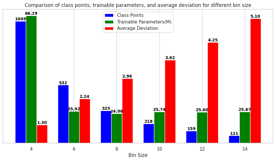
Figure 13: Comparison of class points, trainable parameters, and average deviation for different bin size

TABLE IV: The model structure of the proposed Colorization Network

Layers	Output Size	Kernel	Stride	Outputs
Conv-1	$7\times 7$	$3\times 3$	$1\times 1$	1024
Upsample(scale factor=2)	$14\times 14$	-	-	1024
Conv-2	$14\times 14$	$3\times 3$	$1\times 1$	512
Upsample(scale factor=2)	$28\times 28$	-	-	512
Conv-3	$28\times 28$	$3\times 3$	$1\times 1$	512
Upsample(scale factor=2)	$56\times 56$	-	-	512
Conv-4	$56\times 56$	$3\times 3$	$1\times 1$	532

III-C5 Loss Calculation

Colorization is generally considered a regression problem as the color values are continuous. But we transform the continuous color values into the discrete color classes described in Section III-C1. Therefore, we consider the problem as a classification problem and use cross-entropy loss instead of MSE or other regression loss. The loss function is shown in Equation 13.

$$Loss_{CE}=-\sum_{H,W}\mathcal{W}_{c}\sum_{\mathcal{C}}\mathcal{K}.log(\overline{\mathcal{K}}).$$ (13)

Where $H$ and $W$ are the height and width of output $\kappa$ distribution. $\kappa$ is the true color class and $\overline{\kappa}$ is the estimated color class. The $\omega_{c}$ is the weights vector of color classes. The $\omega_{c}$ is defined as follows in Equation 14.

$$\mathcal{W}_{c}=\Big{(}\frac{1}{n_{\mathcal{C}}}\Big{)},\forall_{c}\in\mathcal{C}$$ (14)

where $N_{c}$ is the number of color classes.

III-C6 Class Confusion Based Weights Adjustment

In realistic images, all color classes are not represented equally. Grayish visual color classes are found in a much larger proportion than bright color classes due to the large background areas. In the categorical cross-entropy loss, each true class gets $\frac{1}{N}$ weight during loss calculation, which is shown in Eq. 14. As the bright color classes are far smaller in the count values, the gradients disappear gradually iteration by iteration. To keep the rarely appearing color classes, we increase the weights of the rarely appearing color classes more than the mostly appearing color classes. However, this process increases the global loss. So the weights need to be trade-offs to ensure both plausible colors and a minimum loss. To trade off the weights, we proposed a new formula, which is given in Equation 15.

$$\mathcal{W}_{\text{new}}=\left(\frac{\sum_{i=1}^{\mathcal{H}}\sum_{j=1}^{\mathcal{W}}\sum_{k=1}^{\mathcal{B}}1}{N^{adj}_{c}+\frac{\max(N_{c})}{\Psi}}\right),\quad\forall c\in\mathcal{C}$$ (15)

where,

$$N^{adj}_{c}=\begin{cases}\Psi&\text{if }N_{c}<\Psi\\ N_{c}&\text{otherwise}\end{cases}\quad\forall c\in\mathcal{C}$$

where,

$$\Psi=\Bigg{(}\frac{\sum_{i=1}^{\mathcal{H}}\sum_{j=1}^{\mathcal{W}}\sum_{k=1}^{\mathcal{B}}1}{n_{\mathcal{C}}}\Bigg{)}\cdot\mathcal{P}(\%)$$

where $\mathcal{H}$, $\mathcal{W}$, $\mathcal{B}$ denote the height, width and batch size of the true class respectively. $\mathcal{C}$ is the color class set, ${\max}(N_{c})$ is the maximum appearance value of a class, $N_{c}$ is the appearance value of class $c$, $\mathcal{W}_{new}$ is the new weights matrix of the particular batch, $N^{adj}_{c}$ is the adjusted appearance value of class $c$, $\Psi$ is the threshold value for adjusting the value of appearance of the classes, $n_{c}$ is the total class number (532 is set by rule) in the optimized class set, $\mathcal{P}$ is the percentage value for determining the $\Psi$.
Initially, we regularize weights by dividing the total count of each class in a batch by its individual appearance value. This ensures that the weight of the most frequently appeared class is set to a minimum while proportionally upscaling the weights of others. However, this approach leads to a significant increase in the weight of classes appearing very infrequently. When a particular class appear 0 or tends to 0 then the weight of that class will be extremely high that makes the learning process imbalance again. To strike a balance, we introduce a trade-off mechanism. Firstly, we adjust appearance value of class $c$ using a threshold factor $\Psi$. By this we prevent every class for being holding extreme high weight. However, some minor classes appear very few times compared to some major classes. Therefore, those major classes go under the domination of some minor classes. To address the problem, we propose an additional term ($\frac{\max(N_{c})}{\Psi}$) for adding to the $N^{adj}_{c}$ term. When the difference between the maximum appeared class and minimum appeared $(\Psi)$ class is very high, the ratio will also be high. Therefore, high value will be added to the adjusted class value. This reduce the weights high appeared classes little but low appeared classes much. This seems little contradictory with our initial target as we are trying to establish the presence of minor class in the generated image and therefore, increasing the weights of the minor classes. However, unrestrained increase of weights of minor class can bias the learning towards minor classes. Our target is to ensure the learning unbiased. Therefore we need a perfect trade-off between the major and minor classes. To address this, we introduce a new hyperparameter $\mathcal{P}$ which denotes how much percentage we will take for determining the value of minimum appeared class. This supplementary term helps control the influence of rare class occurrences, providing a more nuanced and balanced approach to class weight determination. Therefore, the loss function is now modified, as shown in Equation. 16.

$$Loss_{\text{CBCE}}=-\sum_{H,W}\mathcal{W}_{new}\sum_{C}\mathcal{K}.log(\overline{\mathcal{K}}).$$ (16)

Gray

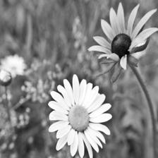
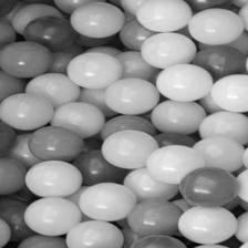
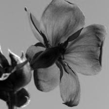
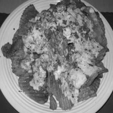
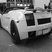
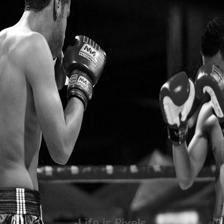
DeOldify[50]

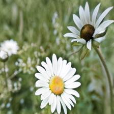
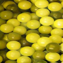
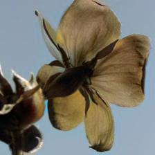
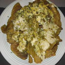
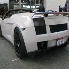
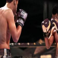
Iizuka[24]

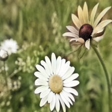
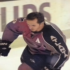
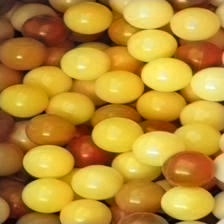
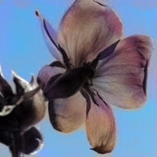
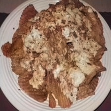
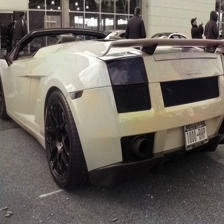
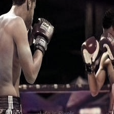
Larsson[20]

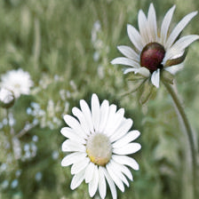
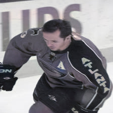
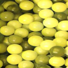
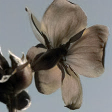
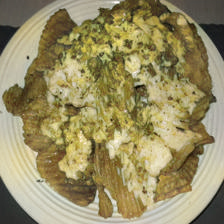
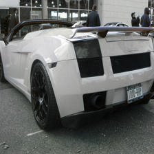
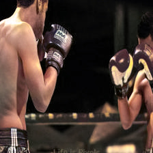
CIC[30]

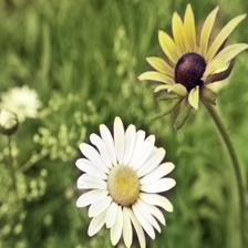
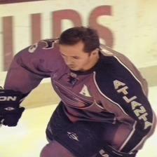
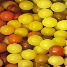
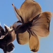
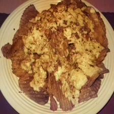
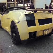
Zhang[34]

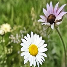
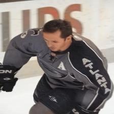
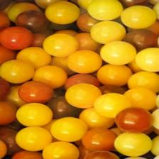
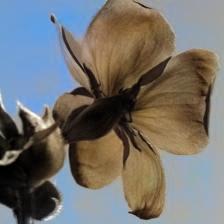
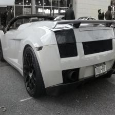
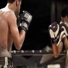
Su[25]

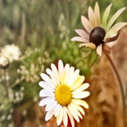
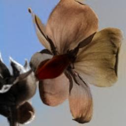
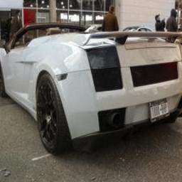
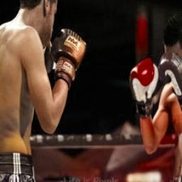
Gain[22]

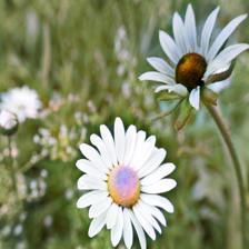
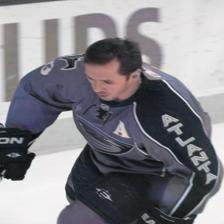
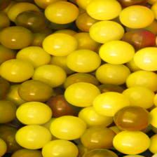
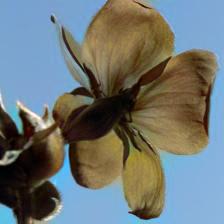
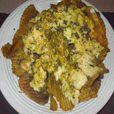
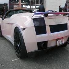
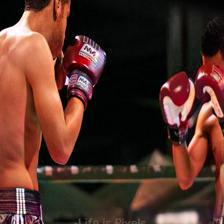
DD[65]

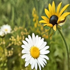
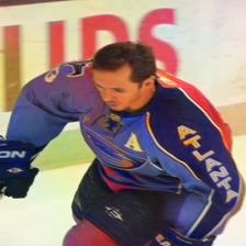
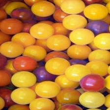
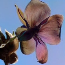
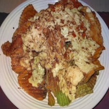
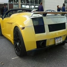
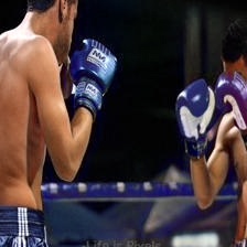
CCC++

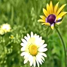
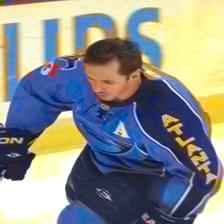
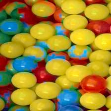
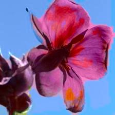
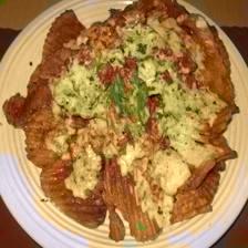
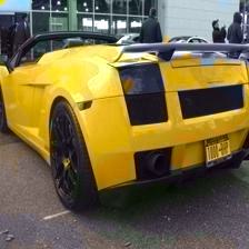
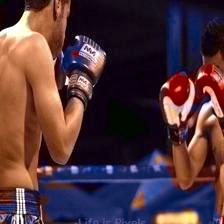
G. Truth

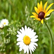
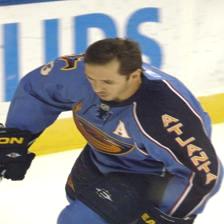
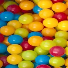
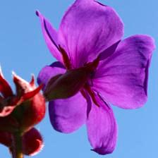
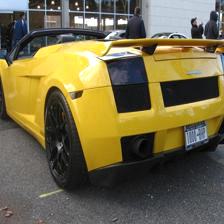
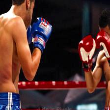
Figure 14: Some results of our proposed method compared to other state-of-the-art methods.

III-C7 Class Probabilities Estimation for Loss Calculation

The network outputs $H\times W\times C\times batch$ tensor. We extract $H\times W\times C\times batch$ softmax probability distribution of the class representation to calculate the loss for backpropagation using the Equation 17.

$$\sigma(\overline{\kappa})_{i}=\frac{e^{\kappa_{i}}}{\sum_{j=1}^{k}{e{\kappa_{i}}}}$$ (17)

III-C8 Class Selection from Probability Distribution for Image Reconstruction

The network outputs a tensor distribution $P$ of dimension $H\times W\times C\times batch$. We extract the class distribution $\mathcal{C}$ of dimension $H\times W\times 1\times batch$ for a*b* color channel construction using the Equation 18.

$$\mathcal{C}\in\mathbb{R}^{H\times W},\quad\mathcal{C}_{ij}=\underset{c}{\operatorname{argmax}}(P_{ijk})$$ (18)

Here, $\quad\mathcal{C}_{ij}$ represents the element at the i-th row and j-th column of matrix $\mathcal{C}$, and it is the index of the maximum probvability along the third dimension of matrix $P$ at the corresponding position.

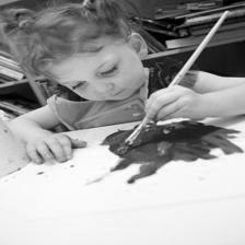
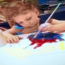
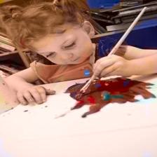
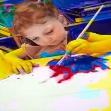
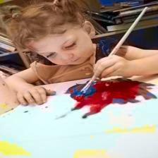
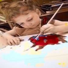
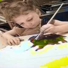
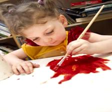
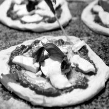
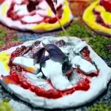
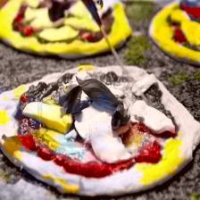
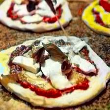
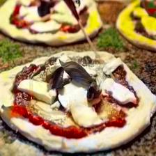
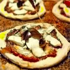
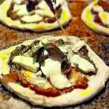
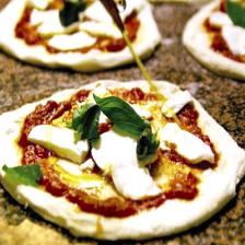
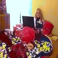
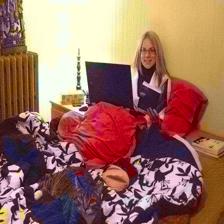
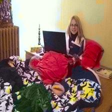
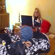
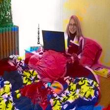
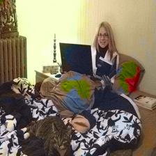
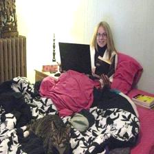
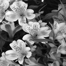
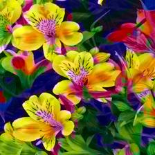
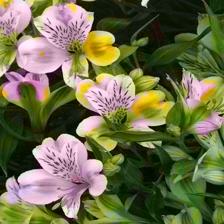
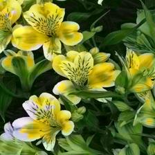
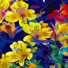
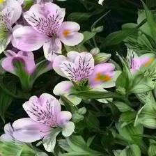
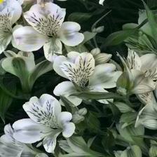
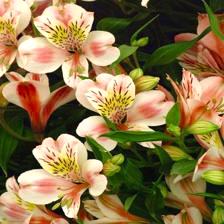
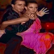
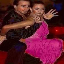
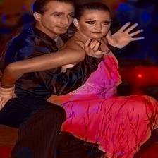
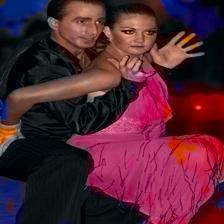
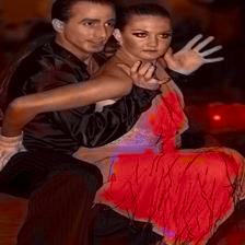
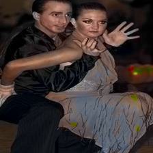
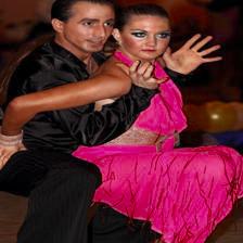
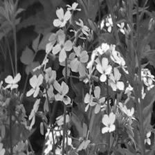
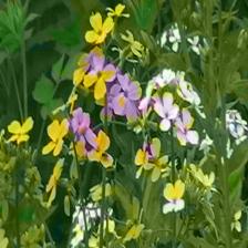
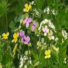
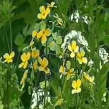
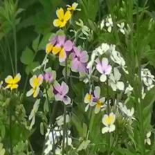
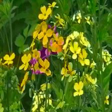
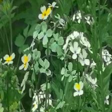
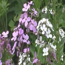
     Gray      bin size = 4    bin size = 6    bin size = 8    bin size = 10    bin size = 12    bin size = 14    Ground Truth

Figure 15: Results on different bin size

III-D SAM Empowered Object-Selective Color Harmonization

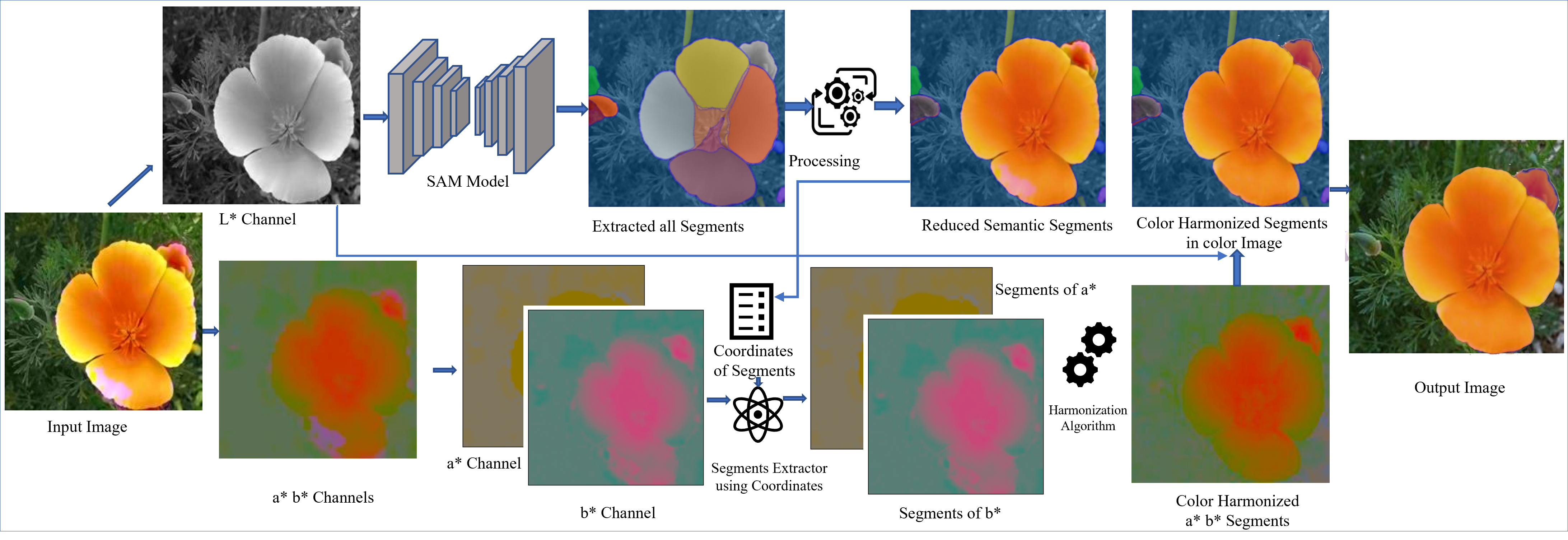
Figure 16: System model for SAM empowered object selective color harmonization.

As we force regularization of the minor class, there is sometimes a little noise at the object’s edge. To make the edge more polished, we proposed SAM-empowered object-selective color harmonization which is shown in Figure 16. The SAM is a segmentation model with zero-shot generalization to unfamiliar objects and images without additional training[53]. The SAM is capable of extracting precise masks for multiple objects from an image[54]. Our proposed algorithm is shown in Algorithm 1.

III-E Chromatic Diversity

Conventional color image assessment metrics often concentrate on measuring discrepancies between generated and ground truth images. However, such metrics may fall short in capturing scenarios where introducing distinctive color accents to specific regions enhances visual aesthetics. Conversely, even a modest area within an image, if strategically aligned with the color scheme of a more dominant counterpart or rendered colorless, can significantly contribute to the conventional measurement criteria. Therefore a small peak ratio (major area only) can give good performance in that criteria and minor areas are overlooked. To address the above mentioned problem, we propose a novel color image evaluation metric named Chromatic Number Ratio (CNR). The CNR quantifies the richness of color classes within the generated images compared to the ground truth images. It offers a comprehensive measure of the spectrum of colors in the generated images, enhancing our understanding of color diversity. The metric is shown in Eq. 19.

$$CNR=\frac{\sum\limits_{i=0}^{m-1}\sum\limits_{j=0}^{n-1}\left(1-\sum\limits_{k=0}^{i-1}\sum\limits_{l=0}^{n-1}[\mathcal{P}_{i,j}=\mathcal{P}_{k,l}]\right)}{\sum\limits_{i=0}^{m-1}\sum\limits_{j=0}^{n-1}\left(1-\sum\limits_{k=0}^{i-1}\sum\limits_{l=0}^{n-1}[\mathcal{G}_{i,j}=\mathcal{G}_{k,l}]\right)}\vspace{-1mm}$$ (19)

where, $\mathcal{P}_{i,j}$ and $\mathcal{G}_{i,j}$ is the color class value at row $i$ and column $j$ of the generated color image $\mathcal{P}$ and Ground truth image $\mathcal{G}$. $m$ and $n$ are the image’s dimensions in the color class space. The outer summation iterates through all rows ($i$) and columns ($j$) of the image in color class space. The inner summation compares each pixel ($\mathcal{P}_{i,j}$ / $\mathcal{G}_{i,j}$) with all previous pixels in the image to check for uniqueness. $[\mathcal{P}_{i,j}=\mathcal{P}_{k,l}]$ and $[\mathcal{P}_{i,j}=\mathcal{P}_{k,l}]$ is an indicator function that returns 1 if the condition is true (if pixel values are equal) and 0 if it’s false.

III-F Color Class Activation Ratio

In the context of Chromatic Number Ratio (CNR), while it effectively quantifies the class activation ratio between generated images and ground truth images, elucidating the precise count of activated color classes within the entirety of discretized color classes poses a challenge. To address the issues, we propose a novel color image evaluation metric named Color Class Activation Ratio (CCAR). The CCAR quantifies percentage of activated color classes in the colorized images . It offers a comprehensive measure of the spectrum of colors in the generated images, enhancing our understanding of color variety. The metric is shown in Eq. 20.

$$CCAR=\frac{\sum\limits_{i=0}^{m-1}\sum\limits_{j=0}^{n-1}\left(1-\sum\limits_{k=0}^{i-1}\sum\limits_{l=0}^{n-1}[\mathcal{P}_{i,j}=\mathcal{P}_{k,l}]\right)}{N_{Class}}$$ (20)

where, $\mathcal{P}_{i,j}$ is the color class value at row $i$ and column $j$ of the generated color image $\mathcal{P}$. $m$ and $n$ are the image’s dimensions in the color class space. The outer summation iterates through all rows ($i$) and columns ($j$) of the image in color class space. The inner summation compares each pixel ($\mathcal{P}_{i,j}$) with all previous pixels in the image to check for uniqueness. $[\mathcal{P}_{i,j}=\mathcal{P}_{k,l}]$ is an indicator function that returns 1 if the condition is true (if pixel values are equal) and 0 if it is false.

III-G True Activation Ratio

In the evaluation metrics CNR (Chromatic Number Ratio) and CCAR (Color Class Alignment Ratio), we effectively quantify the class activation ratio between generated and ground truth images, as well as between generated and total discretized color classes, respectively. However, determining the specific count of color classes that align precisely with ground truth images remains a challenging task. While our primary goal is to enhance the diversity and plausibility of color classes, including those belonging to minor counterparts, we also emphasize the accurate alignment of color classes, particularly focusing on preserving the presence of minor classes. For this, we propose a novel color image evaluation metric named True Activation Ratio (TAR). The TAR quantifies percentage of True activated color classes in the colorized images . It offers a comprehensive measure of the truly selected spectrum of colors in the generated images, enhancing our understanding of color variety. The metric is shown in Eq. 21.

$$TAR=\frac{1}{M}\sum_{j=1}^{M}\frac{1}{N}\sum_{i=1}^{N}I(G_{ji}=T_{ji})$$ (21)

where $G$ be the generated image, $T$ be the ground truth image, and $N$ be the total number of pixels. The pixel-wise matching indicator function $I$ for a pixel at index $i$ is defined as follows:

$$I(G_{ji}=T_{ji})=\begin{cases}1&\text{if }G_{ji}=T_{ji}\\ 0&\text{otherwise}\end{cases}$$

The pixel-wise accuracy for a single image can be expressed as:

$$\textit{Pixel Accuracy}(G,T)=\frac{1}{N}\sum_{i=1}^{N}I(G_{i}=T_{i})$$

Now, considering this for a dataset with $M$ images, the overall Pixel Accuracy $PA$ can be defined as the average accuracy across all images: where, $G_{ji}$ is the intensity value of the pixel at index $i$ in the generated image $j$. $T_{ji}$ is the intensity value of the pixel at index $i$ in the ground truth image $j$, and $I(G_{ji}=T_{ji})$ is the pixel-wise matching indicator function for the pixel at index $i$ in the generated image $j$.

Algorithm 1 SAM Empowered Object-Selective Color Harmonization

0:  Input gray image, Predicted $a^{*}b^{*}$

0:  Edge harmonized a*b*

1:  Extract all segments ($\mathcal{S^{\text{all}}}$) from the gray image using SAM

2:  Pick semantic segments ($\mathcal{S^{\text{sem}}}$) from all the segments ($\mathcal{S^{\text{all}}}$)

3:  for each segment $s$ in $\mathcal{S^{\text{all}}}$ do

4:     Extract $\mathcal{S}^{a}$ from $a^{*}$ using coordinates of $s$

5:     Calculate mode value ($\mathcal{M}_{a}$) of $\mathcal{S}^{a}$

6:     for each pixel ($\mathcal{P}$) in $\mathcal{S}^{a}$ do

7:        if $|\mathcal{P}-\mathcal{M}_{a}|>\delta_{a}$ then

8:           Replace the value of $p$ with $\mathcal{M}_{a}$

9:        end if

10:     end for

11:     Extract $\mathcal{S}^{b}$ from $b^{*}$ using coordinates of $s$

12:     Calculate mode value ($\mathcal{M}_{b}$) of $\mathcal{S}^{b}$

13:     for each pixel ($\mathcal{P}$) in $\mathcal{S}^{b}$ do

14:        if $|\mathcal{P}-\mathcal{M}_{b}|>\delta_{b}$ then

15:           Replace the value of $p$ with $\mathcal{M}_{b}$

16:        end if

17:     end for

18:  end for

19:  return  Edge harmonized a*b*

IV Experiments

This study undertakes several tests to validate the suggested method in this part. Section IV-A describes the datasets used for training and testing. Section IV-B explains the specifics of implementation. Section IV-C introduces evaluation metrics. Two datasets are evaluated quantitatively in Section IV-C3 in comparison to cutting-edge techniques. Section IV-C2 presents the findings of the qualitative analysis. Ablation experiments on the network are given in Section IV-E.

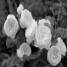
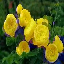
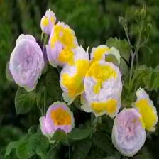
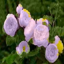
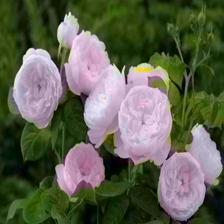
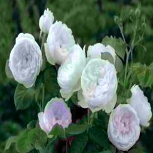
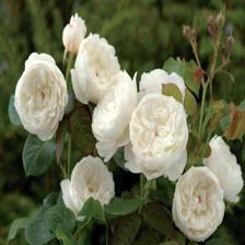
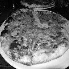
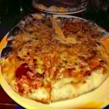
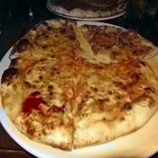
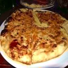
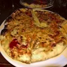
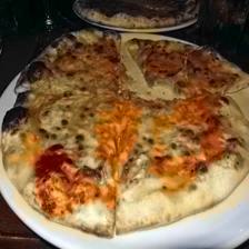
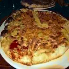
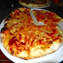
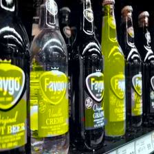
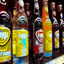
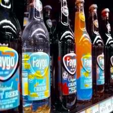
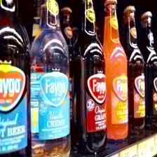
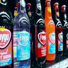
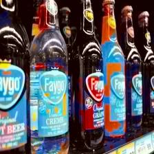
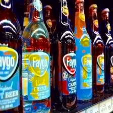
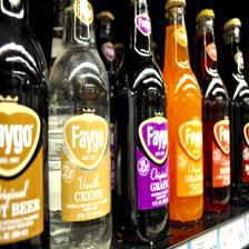
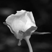
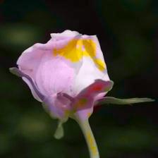
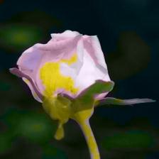
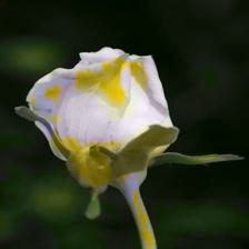
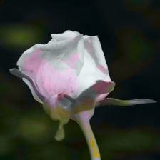
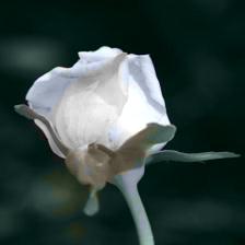
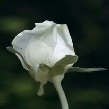
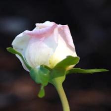
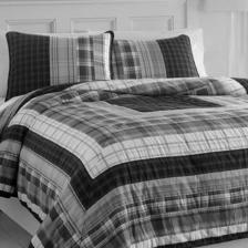
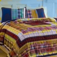
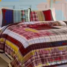
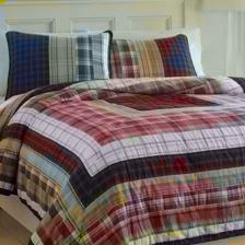
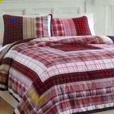
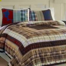
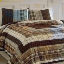
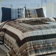
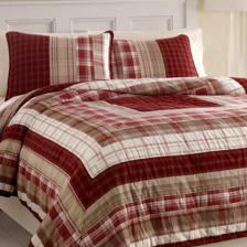
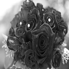
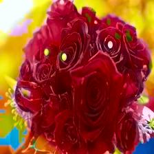
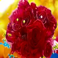
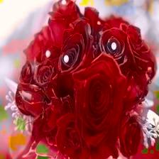
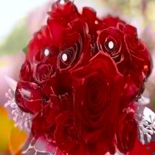
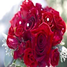
     Gray            4%            6%            8%            10%            12%            14%            16%        Ground Truth

Figure 17: Results on hyperparameters($\mathcal{P}$) testing for determining the value of minimum appeared class for making perfect trade-off between the weights of major and minor classes.

IV-A Datasets

IV-A1 Training

Place365 Train

We train the proposed model using the Place365 Train dataset[32]. 1.8 million images make up the Place365 training set. 365 scene categories with approximately 5000 photos each comprise the Place365 training dataset. We took all images for training our model. Our proposed model is developed on self-supervised manner. We provide no external label of our data during train. Instead, we generate the model’s own supervisory signals or labels from the input data during training.

IV-A2 Testing

Place365 Test

For testing we use the Place365 Test dataset[32]. The dataset has 328.5k images with 365 scene categories. We took all images for testing our model.

ImageNet1k val

The ImageNet1k Validation set is a subset of the ImageNet1k dataset[55]. The dataset is used widely to evaluate the performance of image classification models. It contains 50k images, spanning all 1,000 object classes of main ImageNet dataset. We took all for testing our model.

Oxford 102 Flowers test

Oxford 102 Flower[56] is a set of 102 flower categories used to classify images. The flowers are picked because they are often grow in the UK. Each class consists of a varying number of photographs, ranging from 40 to 258. Large scale, attitude, and light changes are seen in the photographs. To test our model, we used the dataset’s test set. Oxford 102 Flower Test dataset has 819 flower photos in total.

Image Celeba

The CelebFaces(CelebA)[57] dataset consists of 202,599 (2.02M) pictures, encompasses a substantial collection of facial features. The images depict individuals exhibiting various features, such as brown hair, grins, and glasses, among others. Photographs has a substantial capacity to provide extensive visual documentation, including diverse individuals, varied environmental contexts, and a multitude of positional alterations. In order to evaluate our model, a random sample of 50k photographs was chosen from the dataset.

COCO

The Common Objects in Context (COCO)[58] dataset offers an extensive collection of images annotated with object instance segmentation, object keypoints, and dense captions. This dataset encompasses tens of thousands of high-resolution images spanning multiple categories, providing a diverse and comprehensive repository for advancing research in image understanding and scene parsing. The meticulous annotations and broad scope of COCO make it an invaluable asset for researchers, enabling the exploration and development of innovative algorithms in various computer vision tasks, including object detection, segmentation, and image coloring. As a benchmark dataset, COCO plays an important role in facilitating the evaluation and comparison of state-of-the-art models and methodologies, contributing to the ongoing progress and understanding of visual recognition challenges in the field of computer vision.

IV-B Implementation Set Up

The experiments were carried out on a workstation equipped with an NVIDIA GEFORCE RTX 2080 Ti graphics processing unit (GPU). The neural network was implemented using PyTorch[59] version 1.28 in Python 3.10.9. Throughout the training process, we set the batch size to 64 and utilized the Adam optimizer with a learning rate of $1\times 10^{-3}$. The momentum parameters $\beta_{1}=0.5$ and $\beta_{2}=0.999$ were employed for updating and computing the network parameters. To streamline the calculations of our loss function, each ground truth $a*b*$ tensor was resized to a $56\times 56$ dimension. We conducted a systematic exploration of various hyperparameters and trade-off factors for our proposed model, determining their values through meticulous experimental analysis. The specific values are outlined in Tab. V.

IV-B1 Training

During training, the batch size is set to 64, the Adam optimizer is employed with the learning rate $1\times 10^{-3}$, and the momentum parameters $\beta_{1}$ = 0.5 and $\beta_{2}$ = 0.999 are used to update and compute the network parameters. Each of the epochs required for the network training takes approximately 16 hours. Each input gray image was resized to $224\times 224$ pixels. Each ground truth a*b* tensor was resized into $56\times 56$ size for reducing the complexity of loss calculations.

IV-B2 Testing

The batch size is set to 64 for testing purposes. To train the network for color prediction, the input picture is scaled to $224\times 224$, then fed into the network. At the conclusion of the network, the output is deconvoluted to its original size and mixed with the grayscale input $\mathbf{X}$ to produce the created color picture $\mathbf{Y}$. The average values of PSNR, SSIM, IS, and F1D are obtained for quantitative comparison using the produced images and their matching ground truth images.

TABLE V: Different Hyper-parameter and trade-off factor values for CCC++

H. P.	$\alpha$	$\beta$	$\Delta$	$\mathcal{P}$	$\delta_{a}$	$\delta_{b}$	$\Psi$
Value	6	108	36	10	8	8	30

Gray

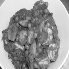
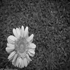
Without Harmonize

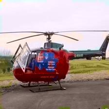
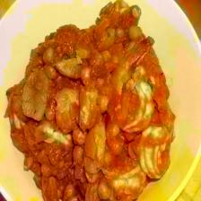
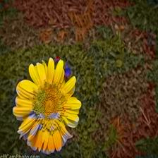
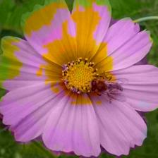
With Harmonize

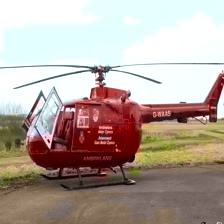
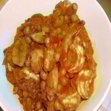
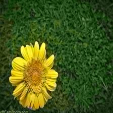
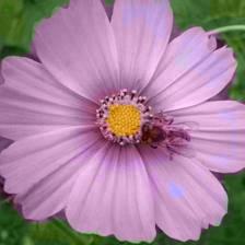
Ground Truth

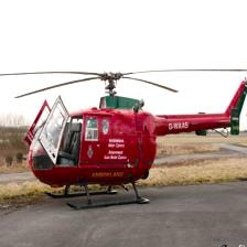
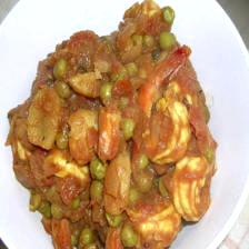
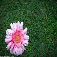
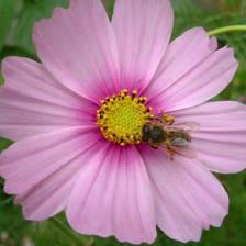
Figure 18: Results with and without color harmonization

IV-C Evaluation Criteria

IV-C1 Evaluation Metrics

We use mean squared error (MSE), peak signal-to-noise ratio (PSNR), structural similarity index measure (SSIM), learned perceptual image patch similarity (LPIPS), universal image quality index (UIQI), and frechet inception distance score (FID) to compare quantitatively our proposed model with the state-of-the-art colorization methods.

Mean Squared Error (MSE)

The MSE[60] is a widely utilized metric in the fields of image processing and machine learning. It quantifies the average squared difference between the values of an estimated or predicted image and the corresponding true or target image which is shown in Equation 22.

$$MSE_{\text{RGB}}(Y,X)=\frac{1}{3N}\sum_{i=1}^{N}(Y_{i}-X_{i})^{2}$$ (22)

where $N$ denotes the number of pixels, $X$ and $Y$ represent the ground truth pixel values and predicted pixel values correspondingly.

Peak Signal-to-Noise Ratio (PSNR)

The PSNR[61] is a commonly employed metric in the field of image and video processing. It serves to assess the quality of a reconstructed or compressed signal by comparing it to the original version which is shown in Equation 23. The signal-to-noise ratio (SNR) quantifies the relationship between the maximum achievable power of a signal and the power of the accompanying noise within that signal.

$$PSNR=10\log_{10}\left(\frac{MAX^{2}}{MSE_{\text{RGB}}}\right)$$ (23)

where $MAX=255$, the maximum pixel value in the RGB scale. The definition of MSE is shown in Equation 22.

Structural Similarity Index (SSIM)

The SSIM[61] is a commonly employed metric within the image and video processing domain which is shown in Equation 24. Its purpose is to evaluate the degree of similarity between two signals. In contrast to metrics such as MSE or PSNR, the SSIM incorporates not only the differences between individual pixels but also considers the structural information and perceptual aspects of the signals.

$$SSIM(Y,X)=\frac{(2\mu_{Y}\mu_{Y}+C_{1})+(2\sigma_{YX}+C_{2})}{(\mu_{Y}^{2}+\mu_{X}^{2}+C_{1})(\sigma_{Y}^{2}+\sigma_{X}^{2}+C_{2})}$$ (24)

where $Y$ is the predicted pixels and $X$ is the ground truth pixels. $\mu_{Y}$ represents the mean of $Y$ and $\mu_{X}$ represent the mean of $X$, $\sigma_{Y}^{2}$ is the variance of $Y$ , $\sigma_{X}^{2}$ is the variance of $X$ , $\sigma_{YX}$ is the covariance of $Y$ and $X$, $C_{1}$ = ${k_{1}L}^{2}$ and $C_{2}$ = ${k_{2}L}^{2}$ are constant values that are used to maintain the stability of SSIM, $L$ is the dynamic range of pixel values, $k_{1}=0.01$ and $k_{2}=0.03$.

Learned Perceptual Image Patch Similarity (LPIPS)

The LPIPS[62] is a metric utilized to quantify the perceptual similarity between images or other visual signals which is shown in Equation 25. In contrast to conventional metrics such as MSE or PSNR, the LPIPS metric incorporates higher-level perceptual characteristics and evaluates similarity based on human perception.

$$d(y,x)=\sum_{l=1}^{L}\frac{1}{H_{l}W_{l}}\sum_{h,w}||(Y_{h,w}-X_{h,w})||_{2}^{2}$$ (25)

where $y$ and $x$ are the predicted image and ground truth image, $d$ is the distance between $y$ and $x$, $l$ is the number of layers in the feature space, $H$ and $W$ are the height and width of feature stacks, $h$ and $w$ are the height and width of the input images and $w$ is the weight vector for converting images to features.

Universal Image Quality Index (UIQI)

The UIQI[63] is a metric utilized to evaluate the quality of an image through a comparison with a reference or ideal image. The UIQI algorithm considers both the structural and statistical characteristics of images in order to calculate a quality score which is shown in Equation 26.

$$Q(Y,X)=\frac{\sigma_{YX}}{\sigma_{Y}\sigma_{X}}\times\frac{2\mu_{YX}}{\mu_{Y}^{2}+\mu_{X}^{2}}\times\frac{2\sigma_{Y}\sigma_{X}}{\sigma_{Y}^{2}+\sigma_{X}^{2}}$$ (26)

where $Y$ is the predicted pixels and $X$ is the ground truth images. $\mu_{Y}$ represents the mean of $Y$ and $\mu_{X}$ represent the mean of $X$, $\sigma_{Y}^{2}$ is the variance of $Y$ , $\sigma_{X}^{2}$ is the variance of $X$ and $\sigma_{YX}$ is the covariance of $Y$ and $X$.

Fréchet Inception Distance (FID)

The FID[64] is a widely utilized metric in the domain of generative adversarial networks (GANs) for assessing the quality and diversity of generated images or samples which is shown in Equation 27. The FID is a metric used to assess the similarity between the distribution of generated samples and the distribution of real samples. The method compares the respective feature representations of generated samples and real samples.

$$FID(X,Y)=|\mu_{X}-\mu_{Y}|+T_{r}(\sigma_{X}+\sigma_{Y}-2\sqrt{\sigma_{X}\sigma_{Y}})$$ (27)

where $Y$ is the feature vector for the predicted image and $X$ is the feature vector for ground truth images, $\mu_{X}$ represents the mean of $X$ and $\mu_{Y}$ represent the mean of $Y$, $\sigma_{X}$ is the covariance of $X$, $\sigma_{Y}$ is the covariance of $Y$ and $T_{r}$ is the rank of the matrix.

TABLE VI: Quantitative comparison of our proposed method with the baseline and SOTA methods using the visuals of Fig. 14.

	MSE $\downarrow$	PSNR $\uparrow$	SSIM $\uparrow$	LPIPS $\downarrow$	UIQI $\uparrow$	FID $\downarrow$	CNR $\uparrow$	CCAR $\uparrow$	TAR $\uparrow$
Deoldify[50]	0.0255	17.15	0.8160	0.2653	0.8618	3.58	0.6054	60.69	5.1499
Iizuka[24]	0.0190	18.09	0.8235	0.2233	0.8553	3.18	0.4383	45.63	4.2966
Larsson[20]	0.0274	16.77	0.8024	0.2815	0.8328	3.93	0.5219	5238	5.9590
CIC[30]	0.0209	18.02	0.8179	0.2258	0.8539	2.41	0.6381	64.47	3.3255
Zhang[34]	0.0250	17.26	0.8197	0.2513	0.8443	3.72	0.5146	51.97	6.3340
Su[25]	0.0233	17.41	0.7908	0.2989	0.8405	2.94	0.6230	63.37	4.5505
Gain[22]	0.0274	16.94	0.8711	0.2569	0.8402	2.73	0.7409	74.53	4.9992
DD[65]	0.0212	18.53	0.8161	0.251	0.8601	1.66	0.9080	95.00	4.9077
CCC++	0.0240	17.88	0.8169	0.2681	0.8517	2.50	1.0507	111.45	7.0256

IV-C2 Qualitative Comnparison

Qualitative evaluation is imperative for assessing the visual prowess of our proposed method. We present a visual ensemble featuring our model’s colorized outputs juxtaposed with grayscale versions, ground truth images, and comparative works from other colorization methods. This visual presentation serves as a comprehensive means to gauge the perceptual fidelity, intricate detailing, and contextual coherence achieved by our proposed method, contributing to a nuanced understanding of its visual performance compared to existing colorization approaches.

In Figure 1, we showed a visual representation of the colorized images of our proposed model along with the gray and ground truth. From the figure, we can see that our proposed model produce very plausible and vivid color compared to the ground truth. In Figure 2, we present a set of six images to elucidate the performance disparities between regression colorization and our proposed classification-based colorization, alongside their grayscale and ground truth counterparts. A discernible distinction emerges from the visual analysis—images generated by the regression model exhibit desaturation and a pronounced grayish tone, whereas those produced by our proposed classification colorization approach showcase vibrant saturation and a diverse color palette. This visual evidence substantiates the superior color richness and diversity achieved by our proposed classification model in comparison to the desaturated outputs of the regression model.

TABLE VII: Regression loss comparison of our proposed method with the baseline and SOTA methods using multiple datasets.

	ADE		COCO		ImageNet		CelebA		Oxford Flower
	MSE $\downarrow$	PSNR $\uparrow$	MSE $\downarrow$	PSNR $\uparrow$	MSE $\downarrow$	PSNR $\uparrow$	MSE $\downarrow$	PSNR $\uparrow$	MSE $\downarrow$	PSNR $\uparrow$
DeOldify[50]	.0043	25.66	0.0067	23.01	0.0136	20.09	.0045	26.06	.0295	16.46
Iizuka[24]	.0035	26.22	0.0067	23.26	0.0115	21.10	.0045	26.00	.0211	18.01
Larsson[20]	.0037	25.94	0.0073	22.34	0.0168	19.26	.0058	26.66	.0245	16.85
CIC[30]	.0053	24.33	0.0075	22.18	0.0109	20.72	.0056	24.79	.0261	17.16
Zhang[34]	.0036	26.07	0.0061	23.32	0.0098	21.61	.0041	26.78	.0295	16.80
Su[25]	.0038	25.37	-	-	0.0116	20.66	.0046	25.70	.0265	16.81
DD[65]	.0039	25.22	0.0071	22.73	0.0097	21.68	.0066	25.70	.0273	16.88
CCC++	.0051	24.53	0.0095	20.74	0.0190	19.12	.0058	24.85	.0181	19.13

In Figure 3, six images are presented, showcasing both full classes and optimized classes colorized outputs, in conjunction with their grayscale and ground truth counterparts. The visual analysis reveals a notable distinction: full class colorization struggles to accurately capture all colors, as the increased number of classes compromises prediction accuracy. Conversely, optimized classes colorization yields more realistic and vibrant color predictions. The precision of the colorization process is enhanced when employing fewer classes, elucidating the trade-off between accuracy and complexity in the optimization of color class predictions.

In Figure 4, we present a series of six images to elucidate the outcomes of the rebalance and nobalance approaches, accompanied by their grayscale and ground truth counterparts. The visual examination reveals a substantial difference: in the nobalance approach, the accuracy of color class predictions is notably low, resulting in a desaturated visual appearance. This can be attributed to an imbalance in the number of desaturated and saturated components within an image. Conversely, the rebalance approach yields saturated and visually plausible results, demonstrating the effectiveness of addressing imbalances in color components for enhanced colorization accuracy.

TABLE VIII: Structural Similarity comparison of our proposed method with the baseline and SOTA methods using multiple datasets.

	ADE		COCO		ImageNet		CelebA		Oxford Flower
	SSIM $\uparrow$	UIQI $\uparrow$	SSIM $\uparrow$	UIQI $\uparrow$	SSIM $\uparrow$	UIQI $\uparrow$	SSIM $\uparrow$	UIQI $\uparrow$	SSIM $\uparrow$	UIQI $\uparrow$
DeOldify[50]	0.96	0.96	0.8631	0.9343	0.9040	0.9006	0.94	0.94	0.82	0.81
Iizuka[24]	0.95	0.96	0.9150	0.9429	0.8918	0.9113	0.95	0.94	0.80	0.82
Larsson[20]	0.95	0.96	0.9021	0.9253	0.8893	0.8910	0.94	0.93	0.82	0.83
CIC[30]	0.95	0.95	0.8599	0.9286	0.9045	0.9053	0.93	0.92	0.81	0.80
Zhang[34]	0.96	0.96	0.8678	0.9374	0.9161	0.9184	0.95	0.93	0.81	0.81
Su[25]	0.92	0.96	-	-	0.8577	0.9094	0.93	0.93	0.77	0.81
DD[65]	0.96	0.96	0.9097	0.9350	0.9074	0.9160	0.93	0.92	0.81	0.80
CCC++	0.93	0.94	0.8860	0.9115	0.8954	0.8802	0.93	0.92	0.81	0.80

In Figures 5(A) and 6(B), a comprehensive comparison is presented, featuring twelve images generated by our proposed CCC++ method alongside a state-of-the-art (SOTA) classification colorization method, in conjunction with grayscale and ground truth images. The analysis from Figure 5(A) reveals that the colorization achieved by our proposed CCC++ method is characterized by more object-specific and saturated hues when compared to the SOTA classification colorization method. Notably, our method exhibits colorized images that closely resemble the ground truth, outperforming the SOTA classification colorization method. Further scrutiny in Figure 6(B) highlights the ability of our proposed method to capture a diverse range of saturated, object-specific colors, including nuanced color details in smaller objects—a distinctive strength when contrasted with the SOTA classification colorization method.

In Fig.14, we compare our proposed CCC++ method with some SOTA colorization method. From the figure we can see that, Deoldify[50] produce overall desaturated color. Iijuka[24] produce some color 3rd, 4th images but overall colorization is trends to grayish effect. Larsson[20] produce overall graish effects. CIC[30] produces some object wise color but not well saturated. Zhang[34] produces some solor in 1st, 3rd, and 6th image but overall desaturated color. Su[25] produces some color in 3rd, 4th, 6th and 8th images but desaturated in others and fully fail to generate color in 2nd and 7th images. Gain[22] produce some color in 4th, 6th and 8th images but overall desaturation. DD[65] produce some good colorization but not object wise plausible. Our proposed CCC++ method produces fully object wise plusible, saturated and vivrant colorization compared to the others and near to the ground truth.

IV-C3 Quantitative Comnparison

In Tab. IX, we evaluate our proposed model against those methods across three datasets using LPIPS and FID criteria. The table shows that our method performs well in all datasets and outperforms others in the ‘Oxford Flower’ dataset. Because ‘Oxford flowers’ dataset has the highest diversity compared to ‘ADE’ and ‘Celeba.’

TABLE IX: Perceptual Image Patch Similarity and frethed image distance comparison of our proposed method with the baseline and SOTA methods using multiple datasets.

	ADE		COCO		ImageNet		CelebA		Oxford Flower
	LPIPS $\downarrow$	FID $\downarrow$	LPIPS $\downarrow$	FID $\downarrow$	LPIPS $\downarrow$	FID $\downarrow$	LPIPS $\downarrow$	FID $\downarrow$	LPIPS $\downarrow$	FID $\downarrow$
DeOldify[50]	0.15	0.48	0.2631	0.5285	0.2216	2.06	0.13	0.43	0.35	3.85
Iizuka[24]	0.16	1.05	0.1939	2.03	0.2218	2.29	0.16	0.45	0.31	3.57
Larsson[20]	0.16	0.62	0.1965	0.8935	0.2561	2.59	0.14	0.37	0.34	2.42
CIC[30]	0.18	1.31	0.2889	2.54	0.2406	2.61	0.17	0.58	0.35	4.20
Zhang[34]	0.14	1.12	0.2538	2.12	0.2081	2.52	0.13	0.49	0.34	4.72
Su[25]	0.21	1.24	-	-	0.2835	2.55	0.18	0.28	0.41	4.51
DD[65]	0.16	0.30	0.1847	0.2049	0.2132	0.65	0.16	0.18	0.32	1.54
CCC++	0.15	0.82	0.2068	1.97	0.2137	1.77	0.13	0.41	0.29	1.49

In Tab. X, we evaluate our proposed model against those methods across five dataset using CNR criteria. The table shows that our method outperforms all methods in all the datasets. The main objective of our proposed model is to ensure the presence of minor colors along with major colors. Minor color confirmation makes color images more diverse because an image contains one or two major colors as well as more minor colors.

TABLE X: CNR, CCAR and TAR comparison of our proposed method with the baseline and SOTA methods using multiple datasets.

	ADE			COCO			ImageNet			CelebA			Oxford Flower
	CNR	CCAR	TAR	CNR	CCAR	TAR	CNR	CCAR	TAR	CNR	CCAR	TAR	CNR	CCAR	TAR
DeOldify[50]	0.77	51.74	5.10	1.43	66.18	3.36	0.61	53.52	4.11	0.62	30.60	9.89	0.69	66.01	1.90
Iizuka[24]	0.78	47.51	2.75	1.49	45.36	2.45	0.49	39.87	1.01	0.51	47.51	2.75	0.58	51.84	1.83
Larsson[20]	0.77	51.24	5.35	0.73	67.30	2.79	0.63	45.23	1.11	0.64	29.38	7.68	0.73	56.13	2.02
CIC[30]	0.81	52.21	2.96	1.57	52.82	2.28	0.58	48.29	2.48	0.86	42.62	4.98	0.67	63.54	1.50
Zhang[34]	0.73	47.75	4.32	1.05	45.70	3.93	0.49	42.28	4.66	0.66	32.58	10.22	0.66	62.87	2.16
Su[25]	0.77	46.31	4.68	-	-	-	0.66	52.93	3.52	0.80	40.93	8.66	0.66	60.11	1.71
DD[65]	1.25	76.83	4.48	2.23	93.73	3.32	0.94	81.17	3.75	1.07	53.37	7.94	0.88	83.67	1.87
CCC++	1.80	77.16	6.25	3.02	92.62	4.28	1.06	86.67	5.31	1.12	67.59	9.44	0.96	85.63	3.15

In Tab. VI, quantitatively evaluate the images of Fig. 14. From the visual and quantitative analysis, we find Deoldify[50] has the best SSIM, Iizuka[24] has the best MSE and PSNR, Larsson[20] has the best UIQI, CIC[30] has the best LPIPS, DD[65] has the best FID, and CCC++ has the best CNR, CCAR, and TAR. Visually, the CCC++ has a more plausible major and minor color combination than the others. Therefore, it is evident that MSE, PSNR, SSIM, LPIPS, and FID criteria are not completely suitable for ensuring the presence of minor colors. Initially prioritizing the optimization of CNR, CCAR, and TAR, followed by the consistent adherence to conventional criteria, emerges as the most effective approach to enhance the representation of both major and minor colors in the generated images.

IV-D Ancient Black and White Photos Colorization

Gray

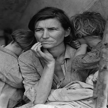
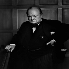
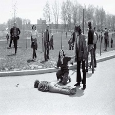
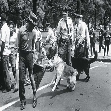
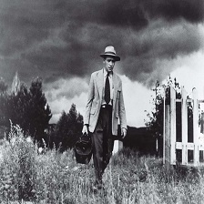
CCC++

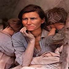
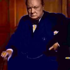
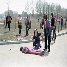
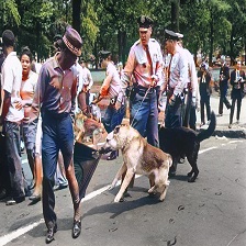
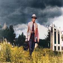
Migrant Mother,1936 Winston Churchill,1941 Kent State Shootings,1970 Birmingham,Alabama,1963 Country Doctor,1948

Figure 19: Black and white historical images and their colorized version by our proposed CCC++ method.

In Tab. VII, we evaluate our proposed model against seven baselines and SOTA methods across three dataset using regression criteria. The table shows that our method performs well in all datasets and outperforms others in the ‘Oxford Flower’ dataset. Since ‘ADE’ predominantly features natural images, while ‘Celeba’ focuses on human faces, typically presenting a more limited range of color combinations. In contrast, the ‘Oxford Flowers’ dataset is characterized by its diverse array of flower species, each exhibiting a unique and varied color palette. This diversity in coloration within the ‘Oxford Flowers’ dataset provides a more complex and challenging environment for colorization, highlighting the efficacy of our method in handling a wide range of colors and complexities.

In Tab. VIII, we evaluate our proposed model against those methods across three dataset using similarity measurement criteria. The table shows that our method performs well in all datasets while maintaining the minor color structure. Usually, it is easier to achieve good similarity by ignoring the minor color features and focusing only on major ones. However, our proposed method maintains satisfactory similarity while ensuring the minor color features.

In the presentation of five historical images alongside their meticulously colorized counterparts generated by our model in Figure 19, a compelling narrative of visual eloquence emerges. These archival photos colors. Our model’s colorization proficiency extends beyond mere aesthetics, demonstrating a keen understanding of historical contexts and nuances. The sepia-toned warmth of vintage photographs and the intricate interplay of hues in landscapes from bygone eras attest to the model’s ability to authentically recreate the colors of yesteryear. This adept infusion of diverse colors not only revitalizes the historical imagery but also serves as a poignant bridge across time, offering a contemporary perspective on moments captured in the past. The seamless integration of varied hues stands as a testament to the nuanced capabilities of our model, fostering a deeper and more resonant connection to the historical narrative embedded within each image.

IV-E Ablation Study

In this section, we rigorously conduct an ablation analysis to systematically dissect and assess the distinct contributions of pivotal components within our proposed model. Illustrated in Figure 13, we offer a comprehensive comparison across various bin sizes, examining class points, trainable parameters, and average deviation. The figure reveals an intriguing trend wherein an increase in bin size corresponds to a decrease in class points and a concurrent rise in average deviation. While bin size 4 exhibits exceptionally high parameters, it also incurs elevated class points. Conversely, other bin sizes demonstrate a trade-off between parameters, class points, and average deviation. After meticulous evaluation, we strategically choose bin size 6 for our proposed model. Despite lower deviations observed in bin size 4, the associated surge in class points and parameters renders it suboptimal. Conversely, although parameters and class points decrease in other bin sizes, a simultaneous increase in average deviation diminishes their viability. In Figure 15, we present a visual representation featuring six distinct images across all bin sizes alongside their grayscale and ground truth counterparts. This visualization underscores the noteworthy correlation between lower bin sizes and heightened saturation, affirming the efficacy of our bin size selection in yielding plausible and vibrant colorization across diverse images.

In Figure 17, we present the results for six different images across seven distinct minimum appearance value determining hyperparameter ($\mathcal{P}$) selection percentages, accompanied by their grayscale and ground truth counterparts. A discernible trend emerges, showcasing that lower percentage selections result in heightened saturation. Specifically, a minimum bin selection of 4% produces a more aggressive and vivid color palette, while the 16% selection yields a softer and less saturated colorization. Since low percentage make makes the minimum appearance value little, the minor start domination over minor. Likewise more percentage makes the minimum appearance of minor value large and the weights of the minor classes increase very little. Striking a balance between saturation and subtlety, we strategically choose a minimum bin selection percentage of 10%. This choice is substantiated by the visual evidence in the figure, where the 10% minimum bin selection consistently delivers colorization characterized by a harmonious blend of saturation, softness, and plausibility, bringing the colorized images closer to the ground truth representations.

In Figure 18, we present a visual comparison featuring five images both with and without color harmonization, alongside their grayscale and ground truth counterparts. It is crucial to note a nuanced aspect here: during the introduction of minor colors into the images, occasional inconsistencies may arise. While such inconsistencies are not ubiquitous, their occasional occurrence necessitates a solution. The figure illustrates instances of color bleeding and inconsistencies in the model output, which are effectively addressed through the application of our color harmonization method. The visual transformation post-harmonization renders the images exceptionally plausible, eliminating inconsistencies and enhancing the overall aesthetic appeal. This nuanced improvement underscores the efficacy of our color harmonization technique in refining the output and ensuring a more coherent and visually pleasing result.

V Conclusion

Automatically colorizing grayscale photographs with objects of diverse colors and sizes presents a formidable challenge due to the intricate variations both within and between objects, compounded by the limited spatial coverage of principal elements. The learning process often grapples with favoring dominant features, thereby yielding biased models. To mitigate this, we introduce a weighted function designed to address feature imbalance, affording greater importance to minority features. In this paper, we put forth a set of formulas facilitating the conversion of color values into corresponding color classes and vice versa. We experiment on different bin size and propose 6 as optimal bin size value. To achieve ideal performance, we strategically optimize the class levels to 532 by experimenting on a large scale of diverse category images and establish a judicious trade-off between the weights assigned to major and minor classes, ensuring accurate class prediction for both. We propose a hyperparameter in the weightening formula to make a balance relation between the weights of the major and minor classes. Additionally, we introduce SAM-empowered object-selective color harmonization, a novel approach enhancing the stability of minor classes. Our contribution extends to proposing two innovative color picture assessment measures, namely Color Class Activation Ratio (CCAR) and True Activation Ratio (TAR), complementing our previously introduced Chromatic Number Ratio (CNR), to quantitatively evaluate color component richness. Extensive evaluations against eight baseline and state-of-the-art models, conducted on six datasets, Place, ADE, Celeba, COCO, Oxford 102 Flower, and ImageNet, reveal that our proposed model outperforms its predecessors across various criteria, including visualization, CNR, CCAR, and TAR, while maintaining commendable performance in regression criteria such as MSE, PSNR, similarity criteria SSIM, LPIPS, UIUI, and generative criteria FID.

Mrityunjoy Gain received the B.S. degree in computer science from Khulna University, Bangladesh, in 2021, where he is currently pursuing the M.S. degree in computer science. His research interests includes continual learning, computer vision, pattern recognition etc.

Avi Deb Raha received the B.S. degree in computer science from Khulna University, Bangladesh, in 2020. Currently he is a PhD student at the Department of Computer Science and Engineering at Kyung Hee University, South Korea. His research interests are currently focused on Deep Learning, Generative AI, Semantic Communication and Integrated Sensing and Communication.

Rameswar Debnath, (Member, IEEE) received the bachelor’s degree (Hons.) in computer science and engineering from Khulna University, Bangladesh, in 1997, and the M.E. degree in communication and systems and the Ph.D. degree from The University of Electro-Communications, Tokyo, in 2002 and 2005, respectively, under the Japanese Government Scholarship. From 2008 to 2010, he was a Postdoctoral Researcher under the JSPS Fellowship with the Department of Informatics, The University of Electro-Communications; the Neuroscience Research Institute; and the National Institute of Advanced Industrial Science and Technology, Tsukuba. From 2012 to 2015, he was the Head of the Computer Science and Engineering Discipline, Khulna University, where he is currently a Professor. His research interests include image data analysis, deep learning, bioinformatics, support vector machine, artificial neural networks, statistical pattern recognition, and medical image processing. He was the Organizing Chair of the 16th International Conference on Computer and Information Technology (ICCIT), in 2014

References

- [1] Y. C. Huang, Y. S. Tung, J. C. Chen, S. W. Wang and J. L. Wu, “An adaptive edge detection based colorization algorithm and its applications”, in Proc. 13th annual ACM international conference on Multimedia, Hilton, Singapore, pp. 351-354, 2005.
- [2] A. Levin, D. Lischinski and Y. Weiss, “Colorization using optimization,” in ACM SIGGRAPH 2004 Papers, Rochester, NY, US: ACM, pp.689–694, 2004.
- [3] L. Yatziv and G. Sapiro, “Fast image and video colorization using chrominance blending,” IEEE Transactions on Image Processing, vol. 15, no. 5, pp. 1120–1129, 2006.
- [4] Y. Qu, T.T Wong, and P.A. Heng, “Manga colorization”, ACM Transactions on Graphics (ToG), vol. 25, no. 3, pp.1214-1220, 2006.
- [5] Q. Luan, F. Wen, D. Cohen-Or, L. Liang, Y.-Q. Xu, and H.-Y. Shum, “Natural image colorization,” In Proceedings of the 18th Eurographics conference on Rendering Techniques, pp. 309-320. 2007.
- [6] T. Welsh, M. Ashikhmin and K. Mueller, “Transferring color to greyscale images,” in Proc. 29th Annual Conference on Computer Graphics and Interactive Techniques, Texas, San Antonio, USA, pp. 277–280, 2002.
- [7] R. Ironi, D. Cohen-Or, D. Lischinski, “Colorization by Example.” Rendering techniques 29, pp. 201-210, 2005.
- [8] Y.-W. Tai, J. Jia and C.-K. Tang, “Local color transfer via probabilistic segmentation by expectation-maximization,” 2005 IEEE Computer Society Conference on Computer Vision and Pattern Recognition (CVPR’05), San Diego, CA, USA, 2005, pp. 747-754 vol. 1, doi: 10.1109/CVPR.2005.215.
- [9] A. Y.-S. Chia, S. Zhuo, R. K. Gupta, Y.-W. Tai, S.-Y. Cho, P. Tan, S. Lin, “Semantic colorization with internet images.” ACM Transactions on Graphics (ToG) vol. 30, no. 6 pp. 1-8, 2011.
- [10] X. Liu, L. Wan, Y. Qu, T.-T. Wong, S. Lin, C.-S. Leung, P.-A. Heng, “Intrinsic colorization,” In ACM SIGGRAPH Asia 2008 papers, pp. 1-9. 2008.
- [11] U. Sousa, R. Kabirzadeh and P. Blaes, “Automatic colorization of grayscale images,” Department of Electrical Engineering, Stanford University, 2013.
- [12] M. He, D. Chen, J. Liao, P. V. Sander, and L. Yuan. ”Deep exemplar-based colorization.” ACM Transactions on Graphics (TOG) vol. 37, no. 4, pp. 1-16, 2018.
- [13] D. Wu, J. Gan, J. Zhou, J. Wang, and W. Gao, ”Fine‐grained semantic ethnic costume high‐resolution image colorization with conditional GAN,” International Journal of Intelligent Systems, vol. 37, no. 5, pp. 2952-2968. 2022.
- [14] Y. Wu, X. Wang, Y. Li, H. Zhang, X. Zhao, and Y. Shan, “Towards vivid and diverse image colorization with generative color prior,” in Proc. IEEE/CVF International Conference on Computer Vision, Montreal, Canada, pp. 14377-14386, 2021.
- [15] M. Wu, X. Jin, Q. Jiang, S.-J. Lee, W. Liang et al., “Remote sensing image colorization using symmetrical multi-scale DCGAN in YUV color space,” The Visual Computer, vol. 37, no. 7, pp. 1707-1729, 2021.
- [16] H. Guo, Z. Guo, Z. Pan, and X. Liu, ”Bilateral res-unet for image colorization with limited data via GANs,” in IEEE 33rd International Conference on Tools with Artificial Intelligence (ICTAI), Manhattan, NY, US: IEEE, pp. 729-735, 2021.
- [17] H. Bahng, S. Yoo, W. Cho, D. K. Park, Z. Wu, X. Ma, and J. Choo, “Coloring with words: guiding image colorization through text-based palette generation,” in Proc. European Conference on Computer Vision (ECCV), Munich, Germany, pp. 431-447, 2018.
- [18] Y. Liang, D. Lee, Y. Li and B.-S. Shin, “Unpaired medical image colorization using generative adversarial network,” Multimedia Tools and Applications, vol. 81, no. 19, pp. 26669-26683, 2022.
- [19] S. Zang, M. Chen, Z. Ai, J. Chi, G. Yang, C. Chen, and T. Yu,“Texture-aware gray-scale image colorization using a bistream generative adversarial network with multi scale attention structure,” Engineering Applications of Artificial Intelligence, vol. 122, pp. 106094, 2023.
- [20] G. Larsson, M. Maire, and G. Shakhnarovich, “Learning representations for automatic colorization,” in European Conference on Computer Vision (ECCV), Midtown Manhattan, NY, US: Springer, pp. 577-593, 2016.
- [21] M. Gain, A. Rahman, R. Debnath, M. M. Alnfiai, A. Sheikh, M. Masud and A. K. Bairagi, “An Improved Encoder-Decoder CNN with Region-Based Filtering for Vibrant Colorization,” Computer Systems Science and Engineering, vol. 46, no. 1, pp. 1059-1077, 2023.
- [22] M. Gain and R. Debnath, ”A Novel Unbiased Deep Learning Approach (DL-Net) in Feature Space for Converting Gray to Color Image,” in IEEE Access, doi: 10.1109/ACCESS.2023.3263948.
- [23] J. An, K. K. Gagnon, Q. Shi, H. Xie and R. Cao, “Image colorization with convolutional neural networks,” in 12th International Congress on Image and Signal Processing, BioMedical Engineering and Informatics (CISP-BMEI), Manhattan, NY, US: IEEE, pp. 1-4, 2019.
- [24] S. Iizuka, E. Simo-Serra, and H. Ishikawa, “Let there be color! joint end-to-end learning of global and local image priors for automatic image colorization with simultaneous classification,” ACM Transactions on Graphics(ToG), vol. 35, no. 4, pp. 1–11, 2016.
- [25] J. W. Su, H. K. Chu and J. B. Huang, “Instance-aware image colorization,” in Proc. IEEE/CVF Conference on Computer Vision and Pattern Recognition, Seattle, WA, USA, pp. 7968-7977, 2020
- [26] J. Dai, B. Jiang, C. Yang, L. Sun and B. Zhang, “Local pyramid attention and spatial semantic modulation for automatic image colorization,” in CCF Conference on Big Data, Midtown Manhattan, NY, US: Springer, pp. 165-181, 2022.
- [27] K. Ruwani M. Fernando, and Chris P. Tsokos, “Dynamically Weighted Balanced Loss: Class Imbalanced Learning and Confidence Calibration of Deep Neural Networks,” In IEEE Trans. Neural Networks and Learning Systems, vol. 33, no. 7, pp. 2940-2951, 2021. doi: 10.1109/TNNLS.2020.3047335.
- [28] D. Hendrycks and K. Gimpel, “A baseline for detecting misclassified and out-of-distribution examples in neural networks,” ICLR, 2017.
- [29] B. C. Wallace and I. J. Dahabreh, “Improving class probability estimates for imbalanced data,” Knowledge and information systems, vol. 41, no. 1, pp. 33–52, 2014.
- [30] R. Zhang, P. Isola and A. A. Efros, “Colorful image colorization,” in European Conference on Computer Vision, Midtown Manhattan, NY, US: Springer, pp. 649–666, 2016.
- [31] M. Gain, A. D. Raha, R. Debnath, “CCC: Color Classified Colorization,” arXiv preprint arXiv:2403.01476 (2023).
- [32] B. Zhou, A. Lapedriza, A. Khosla, A. Oliva and A. Torralba, “Places: a 10 million image database for scene recognition,” IEEE Transactions on Pattern Analysis and Machine Intelligence, vol. 40, no. 6, pp. 1452-1464, 2018.
- [33] M. Xu and Y. Ding, ”Fully automatic image colorization based on semantic segmentation technology,” PloS one, vol. 16, no. 11, pp. 1- 25, 2021.
- [34] R. Zhang, J. Y. Zhu, P. Isola, X. Geng, A. S. Lin, T. Yu, and A. A. Efros, “Real-time user-guided image colorization with learned deep priors,” ACM Transactions on Graphics (TOG), vol. 36, no. 4, pp. 1- 11, 2017.
- [35] E. Reinhard, M. Adhikhmin, B. Gooch, and P. Shirley, “Color transfer between images,” IEEE Computer graphics and applications, vol. 21, no. 5 pp. 34–41, 2001.
- [36] G. Charpiat, H. Matthias, and S. Bernhard, “Automatic image colorization via multimodal predictions.” In Computer Vision–ECCV 2008: 10th European Conference on Computer Vision, Marseille, France, pp. 126-139, 2008.
- [37] R. K. Gupta, A. Y.-S. Chia, D. Rajan, E. S. Ng, and H. Zhiyong, “Image colorization using similar images.” In Proceedings of the 20th ACM international conference on Multimedia, pp. 369-378. 2012.
- [38] A. Bugeau, V. -T. Ta and N. Papadakis, “Variational Exemplar-Based Image Colorization,” in IEEE Transactions on Image Processing, vol. 23, no. 1, pp. 298-307, Jan. 2014, doi: 10.1109/TIP.2013.2288929.
- [39] K. Simonyan and A. Zisserman, ”Very deep convolutional networks for large-scale image recognition,” arXiv preprint arXiv:1409.1556, 2014.
- [40] R. Dahl, “Automatic colorization,” 2016. [Online]. Available: https://tinyclouds.org/colorize.
- [41] J. Hwang and Y. Zhou, “Image colorization with deep convolutional neural networks,” in Stanford University, Tech. Rep., vol. 219, Stanford, CA 94305, United States, pp. 1-7, 2016.
- [42] F. Baldassarre, D. G. Morın, and L. Rodes-Guirao, “Deep koalarization: image colorization using cnns and inception-resnet-v2,” arXiv preprint arXiv:1712.03400, 2017.
- [43] T. -T. Nguyen-Quynh, S. -H. Kim and N. -T. Do, “Image colorization using the global scene-context style and pixel-wise semantic segmentation,” IEEE Access, vol. 8, pp. 214098-214114, 2020.
- [44] J. Yun, S. Lee, M. Park, and J. Choo, “iColoriT: Towards Propagating Local Hints to the Right Region in Interactive Colorization by Leveraging Vision Transformer,” In Proceedings of the IEEE/CVF Winter Conference on Applications of Computer Vision, pp. 1787-1796. 2023.
- [45] M. Hesham, H. Khaled, and H. Faheem, ”Image colorization using Scaled-YOLOv4 detector,” International Journal of Intelligent Computing and Information Sciences, vol. 21, no. 3, pp. 107-118, 2021.
- [46] G. Kong, H. Tian, X. Duan, and H. Long, “Adversarial edge-aware image colorization with semantic segmentation,” IEEE Access, vol. 9, pp. 28194-28203, 2021.
- [47] L. Xia, Z. Qu, J. An, and Z. Gao, ”A Weakly Supervised Method With Colorization for Nuclei Segmentation Using Point Annotations,” in IEEE Transactions on Instrumentation and Measurement, vol. 72, pp. 1-11, 2023, Art no. 4003911, doi: 10.1109/TIM.2023.3265124.
- [48] G. Ozbulak, “Image colorization by capsule networks,” in Proc. IEEE/CVF Conference on Computer Vision and Pattern Recognition Workshops, Long Beach, CA, USA, pp. 0-0, 2019.
- [49] S, Treneska, E. Zdravevski, I. M. Pires, P. Lameski, and S. Gievska, “GAN-based image colorization for self-supervised visual feature learning,” Sensors, vol. 22, no. 4, pp. 1599, 2022.
- [50] J. Antic, “A deep learning based project for colorizing and restoring old images and video!,” 2018. [Online]. Available: https://github.com/jantic/DeOldify.
- [51] A. R. Robertson, “The CIE 1976 color-difference formulae”, Color Research & Application, vol. 2, no. 1, pp.7–11, 1977.
- [52] G. Huang, Z. Liu, L. Van Der Maaten and K. Q. Weinberger, ”Densely Connected Convolutional Networks,” 2017 IEEE Conference on Computer Vision and Pattern Recognition (CVPR), Honolulu, HI, USA, 2017, pp. 2261-2269, doi: 10.1109/CVPR.2017.243.
- [53] Alexander Kirillov, Eric Mintun, Nikhila Ravi, Hanzi Mao, Chloe Rolland, Laura Gustafson, Tete Xiao, Spencer Whitehead, Alexander C. Berg, Wan-Yen Lo, Piotr Dollar, Ross Girshick. Segment Anything. In ICCV, pages 4015-4026, October 2023.
- [54] A. D. Raha,, M. S. Munir, A. Adhikary, Y. Qiao, and C. S. Hong. ”Generative AI-driven Semantic Communication Framework for NextG Wireless Network.” arXiv preprint arXiv:2310.09021 (2023).
- [55] J. Deng, W. Dong, R. Socher, L.-J. Li, K. Li, and L. Fei-Fei, “ImageNet: A Large-Scale Hierarchical Image Database”, IEEE Computer Vision and Pattern Recognition (CVPR), 2009.
- [56] M. Nilsback, and A. Zisserman, “Automated Flower Classification over a Large Number of Classes”, In Proc. Indian Conference on Computer Vision, Graphics and Image Processing, 2008.
- [57] Z. Liu, P. Luo, X. Wang, and X. Tang, “Large-scale CelebFaces Attributes (CelebA) Dataset”, In Proc. International Conference on Computer Vision (ICCV), 2015.
- [58] T.-Y. Lin, M. Maire, S. Belongie, J. Hays, P. Perona, D. Ramanan, P. Dollár, C. L. Zitnick, “Microsoft coco: Common objects in context”, In Computer Vision–ECCV 2014: 13th European Conference, Zurich, Switzerland, September 6-12, 2014, Proceedings, Part V, pages 740-755, 2014.
- [59] A. Paszke, S. Gross, F. Massa, A. Lerer, J. Bradbury, G. Chanan, T. Killeen, Z. Lin, N. Gimelshein, L. Antiga, and A. Desmaison, “Pytorch: an imperative style, high-performance deep learning library,” Advances in Neural Information Processing Systems, vol. 32, 2019.
- [60] Z. Wang and A.C. Bovik, “Mean squared error: Love it or leave it? A new look at signal fidelity measures,” IEEE Signal Processing Magazine, vol. 26, no. 1, pp.98-117, 2009.
- [61] A. Hore´ and D. Ziou, “Image quality metrics: PSNR vs. SSIM,” in 20th International Conference on Pattern Recognition, Manhattan, NY, US: IEEE, pp. 2366–2369, 2010.
- [62] R. Zhang, P. Isola, A. A. Efros, E. Shechtman, and O. Wang, “The unreasonable effectiveness of deep features as a perceptual metric”, in Proc. CVPR, 2018.
- [63] Z. Wang and A. C. Bovik, ”A universal image quality index,” in IEEE Signal Processing Letters, vol. 9, no. 3, pp. 81-84, March 2002, doi: 10.1109/97.995823.
- [64] M. Heusel, H. Ramsauer, T. Unterthiner, B. Nessler, and S. Hochreiter, “GANs trained by a two time-scale update rule converge to a local nash equilibrium”, in Proc. Advances in Neural Information Processing Systems, vol. 30, 2017.
- [65] Xiaoyang Kang, Tao Yang, Wenqi Ouyang, Peiran Ren, Lingzhi Li, Xuansong Xie. DDColor: Towards Photo-Realistic Image Colorization via Dual Decoders. In ICCV. pages 328-338, 2023.