Robot Navigation in Unknown and Cluttered Workspace with Dynamical System Modulation in Starshaped Roadmap

Abstract

This paper presents a novel reactive motion planning framework for navigating robots in unknown and cluttered 2D workspace. Typical existing methods are developed by enforcing the robot staying in free regions represented by the locally extracted ellipse or polygon. Instead, we navigate the robot in free space with an alternate starshaped decomposition, which is calculated directly from real-time sensor data. Additionally, a roadmap is constructed incrementally to maintain the connectivity information of the starshaped regions. Compared to the roadmap built upon connected polygons or ellipses in the conventional approaches, the concave starshaped region is better suited to capture the natural distribution of sensor data (i.e., the starshaped representation generally covers a larger area of the free space), so that the perception information can be fully exploited for robot navigation. In this sense, conservative and myopic behaviors are avoided with the proposed approach, and intricate obstacle configurations can be suitably accommodated in unknown and cluttered environments. Then, we design a heuristic exploration algorithm on the roadmap to determine the frontier points of the starshaped regions, from which short-term goals are selected to attract the robot towards the goal configuration. It is noteworthy that, a recovery mechanism is developed on the roadmap that is triggered once a non-extendable short-term goal is reached. This mechanism renders it possible to deal with dead-end situations that can be typically encountered in unknown and cluttered environments. Furthermore, safe and smooth motion within the starshaped regions is generated by employing the Dynamical System Modulation (DSM) approach on the constructed roadmap. Through comprehensive evaluation in both simulations and real-world experiments, the proposed method outperforms the benchmark methods in terms of success rate and traveling time.

I Introduction

There has been substantial advancement in the field of robot motion planning and control, with applications in diverse areas such as manufacturing, healthcare, agriculture, etc. However, navigating robots in partially or fully unknown environments, particularly in specific regions occupied by many obstacles, remains a significant challenge. In this study, we present a motion planning framework for navigating robots in fully unknown environments. With the proposed approach, safe and fast goal-oriented maneuvers are attained by repeatedly planning for short-term goals on the dynamically constructed starshaped graph and confining the robot motion within the starshaped regions.

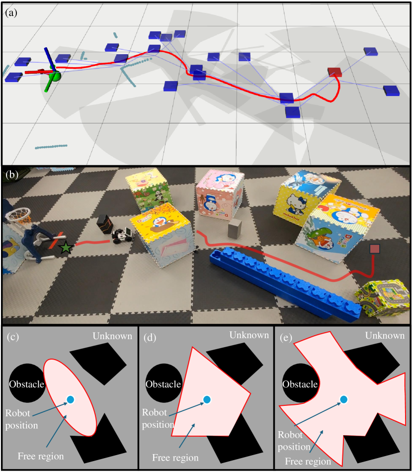
Figure 1: Overview of the proposed reactive motion planning framework. (a) A dynamic starshaped roadmap is constructed to facilitate dynamical system modulation, which enables the robot to navigate from a start position to the goal. (b) With our proposed method, the robot is able to navigate in an unknown and cluttered environment. (c)-(e) Comparing with the representation of free regions by ellipses and polygons, our approach recognizes them as starshaped regions (which capture a larger area of the free space), so that the perception information can be fully exploited for robot navigation.

I-A Related Works

Graph-based searching methods have demonstrated compelling results in the context of collision-free motion planning. Path searching methods, such as A*[1] and D* [2], generally rely on the construction of a graph to describe the free space. Typical graph generation methods include exact/approximate cell decomposition[3], visibility decomposition[4], and Voronoi decomposition[5]. However, deterministic decomposition techniques are computationally demanding or even unavailable in high-dimensional configuration space. On the other hand, sampling-based methods like a probabilistic roadmap (PRM) [6] and rapidly exploring random tree (RRT) [7], can be used to for fast decomposition of the free space by taking random samples and checking the feasibility. Furthermore, substantial variants are proposed to deal with partially unknown or dynamically changing environments by extending existing algorithms with local replanning modules[8, 9, 10]. Remarkably, significant improvements in replanning time and success rate have been achieved in SMART [11] with its informed tree-pruning and tree-repair steps in the replanning process. Also, state-of-the-art navigation systems, such as Far Planner [12] and MUI-TARE[13], are recently developed utilizing graph-based searching methods.

Another category of motion planning methods involves local feedback controllers that utilize real-time onboard sensor data to output control commands reactively. These approaches commonly rely on distance field representations, such as the Euclidean Signed Distance Field (ESDF)[14] and Artificial Potential Field (APF)[15]. The encoded obstacle information can be used directly[16] or fed into an optimization framework[17] to create favorable obstacle-avoiding or goal-reaching behaviors. On the other hand, Dynamical System Modulation (DSM)  [18, 19, 20, 21, 22] has gained popularity in recent years due to its timely obstacle avoidance capabilities. Besides, it has been extended to deal with overlapping convex obstacles [18, 23] and concave obstacles [24] to improve its applicability in dynamic environments with complex obstacles. However, it requires prior knowledge of the obstacle geometries to calculate the modulation matrix and therefore has not been implemented for navigation in fully unknown and cluttered environments yet.

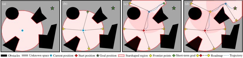
Figure 2: Illustration of the navigation process on the dynamically constructed starshaped roadmap. (a) The roadmap is initialized with the first starshaped region at the start position. (b-c) Frontier points on the starshaped region are generated, and the short-term goal is subsequently selected based on the designed heuristic distance function to the target configuration. A new starshaped free region is extracted upon reaching the current short-term goal if it is extendable. (d) The exploration process is carried on with repeatedly calculated short-term goals till the target configuration is reached.

I-B Our Method

This work is driven by the following considerations. Apparently, navigating robots within locally extracted free regions is computationally efficient in unknown and cluttered environments without requiring any prior knowledge of obstacle geometries. Also, the distribution of point clouds captured by onboard LiDAR can be naturally characterized with starshaped geometry. However, as indicated in Fig. 1(c)- 1(e), existing approaches built upon free regions typically enforce the robot staying in the locally extracted ellipse or polygon (which only utilize part of the sensor information), and thus they typically lead to conservative and myopic behaviors[25, 26]. Furthermore, DSM-based methods are well suited to generating fast reactive collision-free motion even when confronted with intricate obstacle configurations. Yet, to the best knowledge of the authors, there appears to be no existing research that effectively employs DSM on a dynamically constructed roadmap for navigation in environments that are fully unknown and densely populated with obstacles.

With the above considerations as a backdrop, we aim to develop a novel reactive motion planning framework for robot navigation tasks in fully unknown and cluttered environments, leveraging a dynamically constructed starshaped roadmap. We first propose a method to generate the starshaped representation directly from locally perceived point cloud data. Specifically, we represent the point cloud data using polar coordinates, and this facilitates the subsequent fitting process with piece-wise polynomial functions. Then, we build a starshaped roadmap dynamically, in which the frontier points of each region are searched and stored as the potentially extendable positions. During the navigation process, short-term goals are repeatedly selected from those frontier points with minimal distance to the goal configuration, allowing the robot to converge to the target configuration quickly by taking aggressive steps. Notably, the dead-end situations caused by the greedy search method are suitably resolved with a developed replanning mechanism. Furthermore, we customize the DSM method such that it can be applied to mobile robots with circular geometry to generate smooth and efficient motion within the overlapping starshaped free regions. Finally, we implement our proposed motion planning framework in a series of challenging navigation tasks, and the results demonstrate that safe and fast goal-oriented maneuvers are achieved with a high success rate.

II Problem Statement

This work considers a motion planning problem for a robot equipped with an onboard LiDAR to navigate in unknown and cluttered environments. We define the workspace of the robot as $\mathcal{G}\in\mathbb{R}^{d}$, and the workspace contains $M$ obstacles $\mathcal{O}_{i}$, with $i=1,2,\cdots,M$. Notably, different kinds of obstacles including cylinders, connected walls, or other concave obstacles, are involved in the environments, which renders great difficulty in obtaining explicit representations for all the obstacles. In this sense, we consider motion planning in a free space denoted as $\mathcal{W}$ instead, which can be described as:

$$\mathcal{W}=\mathcal{G}-\cup_{i=1}^{M}\mathcal{O}_{i}\in\mathbb{R}^{d}.$$ (1)

Given the initial position $p_{0}\in\mathcal{W}$ and the destination $p_{g}\in\mathcal{W}$, the objective for solving this problem is to formulate a motion planning framework to navigate a robot with a disk-shape in the free space $\mathcal{W}$ based on the locally perceived point cloud information $\mathcal{L}(p)$, where $p\in\mathbb{R}^{d}$ is the position of the LiDAR sensor.

III Methodology

This section introduces details of the proposed reactive motion planning framework, which mainly comprises dynamic roadmap generation and dynamical system modulation within the generated roadmap. The system initially generates starshaped free regions (Sec. III-A1) and frontier points (Sec. III-A2) by utilizing point cloud data, subsequently incorporating DSM (Sec. III-B) to facilitate the robot to navigate within these free regions. Upon reaching a frontier point, the system will determine whether an expansion at the frontier area of the free region is feasible and make corresponding reactions. The loop repeats until the robot successfully arrives at the destination.

III-A Dynamic Roadmap Generation

A roadmap connecting the navigable free regions is typically used to guide the robotic motion in unknown and cluttered environments, especially when facing concave obstacles. This paper proposes a dynamic roadmap $\mathcal{R(N,E)}$, where $\mathcal{N}$ and $\mathcal{E}$ are the node set and edge set of the roadmap, respectively. As shown in Fig. 2, the nodes represent the start position and frontier points, distinguishing the explored and unknown regions. The nodes are incrementally generated during robot motion based on sensor data. On the other hand, edges represent connections between nodes, which means that at least one feasible motion exists between the two connected nodes.

III-A1 Representation of the Starshaped Regions

In order to facilitate the navigation of the robot in unknown and cluttered environments, the starshape is selected to represent the navigable area [27], which is constructed using the perceived point cloud $\mathcal{L}(p)$. Note that $\mathcal{L}(p)$ is preprocessed to add point clouds with the perception range of the LiDAR in the undetected collision-free scope, which construct the rounded edge in Fig. 2 (a). A visual comparison of this method with other free-region representation techniques is shown in Fig. 1(c)-1(e), which illustrates that the starshaped region covers a larger area of the explorable region. A starshaped set $\mathcal{S}(p)\subset\mathbb{R}^{d}$ possesses the property that for every point $p$ in $\mathcal{S}(p)$, there exists at least a reference point $p_{r}$, the line segment between $p_{r}$ and $p$ is confined within $\mathcal{S}(p)$:

$$\exists p_{r}\in\mathbb{R}^{d},\forall p\in\mathcal{S}(p),\ line(p_{r},p)\subset\mathcal{S}(p).$$ (2)

Based on the above definition, the kernel of $\mathcal{S}(p)$, denoted as $ker(\mathcal{S}(p))$, is the set of its reference points $p_{r}$.

An expressive representation of the starshaped region is necessary for the robot navigation tasks, especially when the starshaped region contains various complex obstacles. By utilizing the continuous distance function $\Gamma(p)$, we can discern the geometric relationship between any positions $p$ within the environment and $\mathcal{S}(p_{r})$. The subdomains $\mathcal{H}^{k},k\in\{i,b,e\}$, representing the interior, boundary, or exterior of the starshaped region $\mathcal{S}(p_{r})$ is defined as follows:

$$\begin{array}[]{ll}\text{Interior:}&\mathcal{H}^{i}=\left\{{p}\in\mathbb{R}^{d}:\Gamma\left({p}\right)>1\right\},\\ \text{Boundary:}&\mathcal{H}^{b}=\left\{{p}\in\mathbb{R}^{d}:\Gamma\left({p}\right)=1\right\},\\ \text{Exterior:}&\mathcal{H}^{e}=\left\{{p}\in\mathbb{R}^{d}:\Gamma\left({p}\right)<1\right\}.\end{array}$$ (3)

Given a reference point $p_{r}\in ker(\mathcal{S}(p))$, if we represent the starshpaed set generated by $\mathcal{L}$ as a free region, the distance function gradually decreases from positive infinity at $p_{r}$ and then along the radial direction. The function is described as:

$$\Gamma(p)=\left\{\begin{array}[]{ll}\left(R(p)/\left\|p-p_{r}\right\|\right)^{\sigma}&p\neq p_{r}\\ \infty&p=p_{r}\end{array},\right.$$ (4)

where $R(p)$ is the distance to the boundary of $\mathcal{S}(p)$ along the direction from $p_{r}$ to $p$, and it is also referred to as the radius of $\mathcal{S}$. The weight parameter is denoted as $\sigma$.

To effectively utilize the above features of the starshaped sets as a continuous function to navigate the robot, it is necessary to parameterize the starshaped regions to calculate the modulation matrix required by the DSM method. In this paper, for a 2D environment, we transform the point cloud $\mathcal{L}(p)$ from the Cartesian coordinate system into a polar coordinate system, with the origin of the point cloud $p$ serving as one valid reference point $p_{r}$. Specifically, we map the positions $p_{l}=(p_{x,l},p_{y,l})$ to the vector $(\theta,r)$. For any position within the region except $p_{r}$, the transformation formulation is given by:

$$\left[\begin{array}[]{l}\theta\vspace{0mm}\\ r\end{array}\right]=\left[\begin{array}[]{c}\arctan(p_{y,l}-p_{y,r},p_{x,l}-p_{x,r})\vspace{1.5mm}\\ \sqrt{(p_{y,l}-p_{y,r})^{2}+(p_{x,l}-p_{x,r})^{2}}\end{array}\right].$$ (5)

To facilitate the process of fitting the starshaped region, we introduce an adaptive segmentation algorithm that relies on the change rate in distance $R(p)$, to construct a piecewise $i$th-order polynomial function. The polynomial for each segment is described as:

$$r(\theta)=a_{0}+a_{1}\theta+a_{2}\theta^{2}+\cdots+a_{N}\theta^{N}=\sum_{i=0}^{N}a_{i}\theta^{i}.$$ (6)

The piecewise function, consisting of the above polynomials, is described as:

$$\sum_{k=1}^{M}\mathcal{P}_{k}=\left\{\begin{array}[]{cc}\sum_{i=0}^{N}a_{i,1}\theta^{i},&\theta\leq\theta_{1}\vspace{1.5mm}\\ \sum_{i=0}^{N}a_{i,2}\theta^{i},&\theta_{1}<\theta\leq\theta_{2}\vspace{1.5mm}\\ \cdots&\vspace{1.5mm}\hfil\\ \sum_{i=0}^{N}a_{i,k}\theta^{i},&\theta_{k-1}<\theta\leq\theta_{k}\\ \end{array}.\right.$$ (7)

The segmentation points $\theta_{i}$ are determined by analyzing the change rate in distance between adjacent points. Specifically, we identify points where the change rate exceeds a predefined threshold.

III-A2 Frontier Points Generation in a Starshaped Set

Firstly, for the point cloud $\mathcal{L}(p)$, we eliminate the points with the maximum detected range. Next, we employ the DBSCAN [28] algorithm to cluster the remaining points and eliminate outliers. We then extract the points within each cluster, referred to as side points in this paper. Each cluster’s pair of side points represent the two outermost points with the maximum and minimum angles in polar coordinates, recorded by their angular values $\theta_{s}\in[-\pi,\pi]$. Finally, we connect adjacent side points from neighboring clusters and calculate the geometric midpoint as the frontier points, signifying the boundary between the explored and unexplored regions of the environment. The mathematical expression of each frontier point is an angular value $\theta_{f}=\frac{\theta_{s1}+\theta_{s2}}{2}\in\mathcal{F(S)}$, where $\theta_{si},i\in\{1,2\}$ are the angle of the two side points, and $\mathcal{F(S)}$ represents the set of frontier points of the starshaped set $\mathcal{S}(p)$. Note that although the frontier points are calculated by the angle value of the point clouds, we still can easily get the corresponding Cartesian coordinate by using (5).

With the above definitions and analysis, the roadmap $\mathcal{R(N,E)}$ is initialized as follows: the first node $n_{0}\in\mathcal{N}$ of the roadmap is designated as the start position of the robot, and a starshaped region is created, the generated frontier points $n_{i}\in\mathcal{N}$ are added to the roadmap. The edges $e_{i}\in\mathcal{E}$ between $n_{0}$ and $n_{i}$ are recorded. Specifically, if two nodes are included in the same starshaped region, an edge connecting them is established. Using a heuristic search method, a short-term goal $p_{s}$ is selected from $n_{i}$. The control input utilized by the robot to navigate towards the short-term goal is modulated based on the above representation of a starshaped set containing the short-term goal, which will be described in Section III-B.

III-A3 Short-Term Goal Selection and Roadmap Update

To navigate through unknown and cluttered environments with concave obstacles, we ensure the robot always has a reachable short-term goal by navigating in starshaped regions. Once a new starshaped set is successfully constructed at the location of the last short-term goal, the robot generates a new starshaped set, and its corresponding frontier points, which are added to the set of frontier points $\mathcal{F}(\mathcal{S}_{i})\subseteq\mathcal{F},i\in\{1,2,\cdots,N_{\mathcal{S}}\}$, where $N_{\mathcal{S}}$ represents the number of constructed starshaped sets. In this paper, we propose a general short-term goal selection approach. Given arbitrary start and end positions, a sequence of short-term goals is searched from the frontier point set $\mathcal{F}$ in the roadmap to guide the robot step by step towards the goal position. We denote the short-term goals as $p_{s,j}\in\mathcal{F}$, where $j\in\{1,2,\cdots,N\}$. Here, $N$ means the number of selected short-term goals in one search process. To get the list of a short-term goal set $\mathcal{Z}(p,p_{g})=\{p_{s,1},p_{s,2},\cdots,p_{s,N}\}$, we present the following optimization problem, as a heuristic of the short-term goal selection task:

$$\begin{array}[]{cc}\underset{{p_{s,1},p_{s,2},\cdots,p_{s,N}}}{\min}&\sum_{i=1}^{N}\|p_{s,i}-p_{s,i-1}\|\\ \text{s.t.}&p_{s,N}=p_{g},\\ &(p_{s,i},p_{s,i+1})\in\mathcal{E},\end{array}$$ (8)

where the second constraint means that $p_{s,i}$ and $p_{s,i-1}$ construct an edge in the roadmap.

Every short-term goal $p_{s}$ in the roadmap is characterized by two distinct attributes: extendable and stuck. These attributes are assigned to the respective short-term goal when the robot reaches it. Specifically, if the robot can pass through the unexplored space from the current $p_{s}$, it is designated as extendable. At the same time, a new starshaped set and its corresponding frontier points are generated based on the current information $\mathcal{L}(p)$ perceived from the onboard LiDAR. On the other hand, if the robot cannot pass through the frontier point to explore the remaining unknown environment, the short-term goal is assigned the attribute stuck, indicating that the robot needs to find an alternative route to the destination. Additionally, this stuck frontier point and its corresponding edges to other nodes are removed from $\mathcal{E}$, ensuring that this point is not selected as a short-term goal in the future motion planning process. Meanwhile, the roadmap will update at the current location of the robot, and a new list of short-term goals is generated by solving (8) to provide a feasible coarse path and escape this dead-end. The robot then moves along the short-term goal in the list until a new list needs to be generated. This process is repeated until the robot reaches the destination $p_{g}$.

In summary, during the robot’s navigation process, the roadmap is dynamically updated by adding, deleting, and continuously detecting new frontier points. The corresponding edges are also recorded in the dynamic roadmap.

Input: $p$, $p_{g}$, $\mathcal{L}$ and $\mathcal{R}$

Output: $u$ and $\mathcal{R}$

1 Function GenRoadmap($p,\mathcal{L},\mathcal{R}$):

2       $\mathcal{P}\leftarrow$ Fit piecewise polynomial with $\mathcal{L}$;

3       $\mathcal{F}\leftarrow$ Identify frontier points with $\mathcal{L}$;

4       $\mathcal{N}\leftarrow$ $p$ and $\mathcal{F}$;

5       $\mathcal{E}\leftarrow$ Constructing edge set in $\mathcal{N}$;

6       $\mathcal{R}^{*}\leftarrow$ Build the roadmap with $\mathcal{N}$ and $\mathcal{E}$;

7       $\mathcal{R}\leftarrow\mathcal{R}\cup\mathcal{R}^{*}$;

8       return $\mathcal{R}$

9

10Initialize $\mathcal{R}$ as $\emptyset$ and $p_{s}$ does not exist;

11 while $p\neq p_{g}$ do

12       if $\mathcal{R}$ is $\emptyset$ or $p=p_{s}$ or update then

13             $\mathcal{R}\leftarrow$ GenRoadmap($p,\mathcal{B},\mathcal{R}$)

14       end if

15      

16      $p_{s}\leftarrow$ Search in the roadmap $\mathcal{R}$;

17       stuck $\leftarrow$ Check the feasibility of $p_{s}$;

18       if stuck then

19             Delete $p_{s}$ in $\mathcal{R}$;

20             replan, update $\leftarrow$ $True$

21       end if

22      if $p=p_{g}$ or replan then

23             Continue;

24            

25       end if

26      $\tilde{p}^{*}$, $\tilde{p}_{n}^{*}\leftarrow$ Get modulated velocity vector with $p_{s}$ using (19);

27       $\tilde{p}^{*}\leftarrow$ Get combined velocity vector using (20);

28       $u\leftarrow$ Get control input with (9)

29 end while

Algorithm 1 Reactive Motion Planning with DSM in Starshaped Roadmap

III-B Dynamical System Modulation in Starshaped Roadmap

III-B1 Collision Free Motion Model

The robot is modeled as a disk-shaped differential drive agent with a radius of $R$. The state of the robot is represented by the vector $z=(p,{\theta})\in\mathbb{R}^{3}$, where $p=(p_{x},p_{y})\in\mathbb{R}^{2}$ is position, and ${\theta}$ denotes the heading angle relative to the $x$-axis of the global frame. The control input of the robot is defined as $u=(v,\omega)\in\mathbb{R}^{2}$, where $v$ represents the linear velocity and $\omega$ represents the angular velocity. The robot generates the control input $u$ using the low-level controller:

$$u=f(z,\tilde{p}),$$ (9)

where $f(\cdot)$ is a continuous function generating the control command. $\tilde{p}$ is a velocity vector from the current robot state to the desired position $p_{s}$ described as:

$$\tilde{p}=[p_{s,x}-p_{x},p_{s,y}-p_{y}]^{\top}\in\mathbb{R}^{2}.$$ (10)

In this method, the above control command considers the short-term goal as a desired position, so we use DSM to modulate the robot with collision avoidance in the starshaped regions:

$${\tilde{p}^{*}}=\mathbf{M}(z)\tilde{p},$$ (11)

where $M(z)$ is the modulation matrix applied to adjust the motion direction, thereby enabling obstacle avoidance by preventing the robot from reaching the detected boundary of the specified starshaped regions.

Remark 1

Utilizing DSM for obstacle avoidance necessitates prior knowledge of the shape or formulation of the obstacles [18, 23], rendering the method infeasible for fully unknown environments. To address this issue, we construct the aforementioned dynamic roadmap of the free region online.

III-B2 Short-Term Goal Navigation within One Starshaped Area

To guide the robot towards the assigned short-term goal while ensuring collision avoidance, DSM is employed to modulate the initial velocity vector of the robot generated by (10). The modulation matrix in (11) is designed to guide the movement of the robot to $p_{s}$ while taking into account obstacle avoidance. The matrix $\mathbf{M}(p)$ is described as follows:

$$\mathbf{M}(p)=\mathbf{E}(p)\mathbf{D}(p)\mathbf{E}(p)^{-1},$$ (12)

where $\mathbf{E}(p)$ and $\mathbf{D}(p)$ represent the basis matrix and the diagonal matrix with entries of the corresponding eigenvalues, respectively. These matrices are defined as

$$\begin{split}\mathbf{E}(p)&=[\mathbf{r}(p)^{\top},{\mathbf{e}_{1}(p)^{\top},\cdots,\mathbf{e}_{d-1}(p)^{\top}}_{d-1}]^{\top}\in\mathbb{R}^{d\times d},\\ \mathbf{D}(p)&=\operatorname{diag}[\lambda_{r}(p),\underbrace{\lambda_{e}(p),\cdots,\lambda_{e}(p)}_{d-1}]\in\mathbb{R}^{d\times d},\end{split}$$ (13)

where $\mathbf{r}_{p}=p_{r}-p$ denotes the reference direction. $\mathbf{e}_{i}(p)$ represents the tangential direction to the gradient $\partial\Gamma(p)/\partial{p}$ at the $i$th dimension. In this paper, $\mathbf{e}_{i}(p)$ represents the normal direction on the boundary of the starshaped region. According to the analytical expression of the parameterization of starshaped sets in Section III-A1, the vector of the normal direction can be calculated by:

$$\mathbf{e}_{i}=[\cos(\bar{\theta}_{i}),-\sin(\bar{\theta}_{i})]^{\top},$$ (14)

where,

$$\bar{\theta} =\frac{\dot{r}(\theta)\sin(\theta)+r(\theta)\cos(\theta)}{\dot{r}(\theta)\cos(\theta)-r(\theta)\sin(\theta)},$$ (15)

$$\theta =\arctan(p-p_{r}).$$ (16)

Here, $\dot{r}(\theta)$ denotes the first order derivative of (5) with respect to $\theta$. Besides, $\lambda_{j}$ is the modulation weight of the corresponding direction at the $j$th dimension, and the eigenvalues $\lambda_{j}(p),j\in\{r,e\}$ are calculated by:

$$\lambda_{j}(p)=\left\{\begin{array}[]{ll}\lambda_{r}(p)=1-1/\Gamma(p)&j=r,\\ \lambda_{e}(p)=1+1/\Gamma(p)&j=e.\end{array}\right.$$ (17)

III-B3 Short-Term Goal Navigation in An Overlapped Area of Several Starshaped Regions

As shown in Fig. 2 (d), when the robot travels in the environment, it may encounter overlapped areas of multiple starshaped regions, resulting in several basis and eigenvalue matrices. Therefore, it is necessary to calculate weights from the multiple starshaped sets to ensure the robot can be guided through the overlapped area.

In each starshaped set $\mathcal{S}_{k}(p),k\in\{1,2,\cdots,N\}$, a modulated velocity vector $\tilde{p}_{k}$ is calculated using (11). With a slight abuse of notations, $N$ is denoted as the number of overlapped starshaped regions. The weight of each starshaped set is determined based on the value of their own $\Gamma_{k}(p)$ and summed weight in the overlapped area:

$$w_{k}(\boldsymbol{p})=\frac{\max\left\{\Gamma_{k}(\boldsymbol{p}),1\right\}}{\sum_{i=1}^{N}\max\left\{\Gamma_{i}(\boldsymbol{p}),1\right\}}.$$ (18)

Incorporating the weights of the starshaped sets present in the overlapped area, the overall control input $\tilde{p}^{*}$ of the robot in the overlapped area can be expressed as:

$$\tilde{p}^{*}=\sum_{k=0}^{N}w_{k}\mathbf{M}_{k}(z)\tilde{p}.$$ (19)

Considering the disk-like shape of the robot, in addition to the center position of the robot, we utilize the nearest point $p_{n}$ in the received point cloud $\mathcal{L}(p)$ as an additional guidance point. By combining the modulated velocity vector generated by the position at the center of the robot, we obtain a merged velocity vector ${p}^{*}$ calculated by:

$${p}^{*}=(1-\alpha)\tilde{p}^{*}+\alpha\tilde{p}_{n}^{*},\quad\alpha=\min\left(\frac{\rho}{d-R},1\right),$$ (20)

where $\rho$ is a predefined parameter.

With the above processes, the robot is able to navigate in a totally unknown environment without collision with obstacles with different geometries. For ease of understanding, the overall algorithm of the proposed method is illustrated in Algorithm 1.

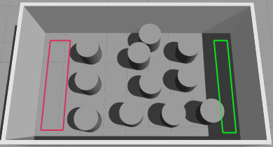
(a) Forest

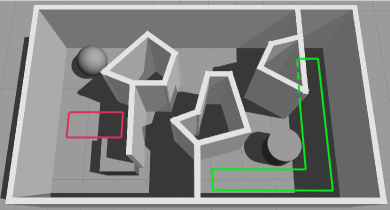
(b) Maze

Figure 3: Simulation scenarios for obstacle avoidance testing. (a) A forest-like cluttered scenario with cylindrical obstacles. (b) A challenging maze-like scenario with spherical, cylindrical, and concave obstacles. The random start and target positions will be generated in the corresponding red and green regions in the simulation experiments.

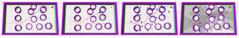
(a) Navigation results in forest scenario.

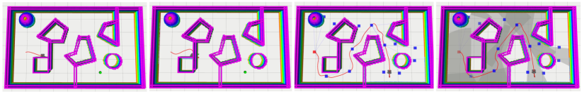
(b) Navigation results in maze scenario.

Figure 4: Simulation results in the constructed scenarios, with the methods used from left to right being DSM [18], FOA [22], FOA with RM, and our approach. (a) In the forest environment, all methods except for FOA enable the robot to successfully navigate to the destination. (b) In the maze environment, both DSM and FOA fail to enable the robot to reach the goal position. Our approach effectively addresses both environments.

IV Simutation and Experiment Results

This section compares our proposed reactive motion planning method with other approaches, including DSM[18], FOA[22], and FOA with our proposed roadmap (FOA with RM). The evaluation criteria include travel time, path length, computation time, and success rate. The performance evaluation is divided into two parts: simulation with multiple cluttered and representative workspaces in the Gazebo simulator and experiment in a real-world dense obstacle avoidance scenario using a differential drive mobile robot. Both environments are built on Python 3.10 on a 2.3GHz Intel i7-12700H processor. In the real-world experiment, the onboard computer of the mobile robot perceives the environment with a 360^∘ 2D LiDAR and communicates with the host computer. After the modulated velocity vector is calculated by (19), a PID controller is used to control the motion of the robot.

TABLE I: Comparison of the navigation performance

Scenario	Method	TTR Avg. (%)	PLR Avg. (%)	SR (%)
Forest	DSM[23]	89.8	102.14	73.3
	FOA[22]	99.6	109.9	20.7
	FOA with RM	137.0	108.6	40
	Ours	100	100	90
Maze	DSM[23]	–	–	0
	FOA[22]	–	–	0
	FOA with RM	115.8	94.9	80
	Ours	100	100	83.3

IV-A Simulation Evaluation

To evaluate the effectiveness and versatility of our proposed reactive motion planning method, we conduct simulations using the Gazebo simulator. Two cluttered and representative workspaces are used to ensure a comprehensive evaluation of the performance of the algorithm. To create the simulated environments, we utilize various predefined 2D models representing common obstacles in real-world scenarios, such as walls and irregularly shaped objects.

For each scenario, we generate different initial robot poses and goal locations and repeat the experiment 30 times in each scenario, as shown in Fig. 3, enhancing the complexity of the environment and the traversal paths. The proposed reactive motion planning algorithm and other methods are then applied to navigate the robot from the initial pose to the goal with a velocity of 0.5 m/s in the unknown environment. We define two performance metrics to quantify the results, the travel time ratio (TTR) and path length ratio (PLR). Note that TTR and PLR represent the ratio of travel time/path length achieved with benchmark methods and ours. As presented in Table I, the average of TTR, PLR, and success rate (SR) are recorded in the experiments for those successfully reaching the goal configuration.

IV-A1 Forest Scenario

The scenario has convex obstacles, like cylinders with a radius of 0.5 m, with uneven distribution. Note that in this case, DSM needs to know the exact shape and location of the obstacles to work correctly. The environment is completely unknown for other methods. Our method has the highest success rate compared to other methods. Even though the DSM navigates the robot with prior environment information, the two cylinders in close contact with each other will result in a local minimum that will cause the robot to fail to reach the goal. But the roadmap we built online can facilitate better performance in escaping from the local minima. The FOA often encounters saddle points, making it impossible to avoid obstacles in time. Even with the guidance of the roadmap, the success rate is not improving significantly.

IV-A2 Maze Scenario

In the unknown and cluttered maze scenario, both the DSM and the FOA are unable to drive the robot to the goal configuration due to the complexity of the obstacles. For DSM, since it is challenging to express complex obstacles using functions, it is impossible to compute the modulation matrix directly in such an environment. At the same time, FOA cannot cope with this environment because it relies only on sensor data from the current frame. However, the performance of FOA has been significantly improved after the combination with the starshaped roadmap proposed in this work. However, our method achieves faster navigation and a higher success rate with minimal compromise in the traversal length.

In terms of the computation time, the average result in our proposed starshaped roadmap is $3.98\pm 0.96$ ms and $4.37\pm 1.16$ ms in the forest and maze scenarios, respectively. The computational efficiency allows us to set a high control frequency for the robot to make timely reactions to the unknown environment. Although the fitting process for the starshaped representation takes approximately $0.15$ s, it only needs to be executed when expanding the roadmap, and thus it has minimal impact on the overall computational efficiency of the proposed algorithm.

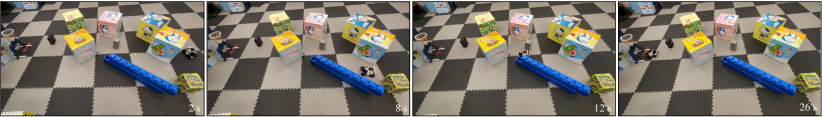
(a) Snapshots in the robot navigation process.

(b) Visualization of the roadmap generation and the trajectory of the robot.

Figure 5: Real-world experiment conducted on a differential drive mobile robot. We successfully navigate the robot through an unknown and cluttered environment utilizing the incrementally built starshaped roadmap. In particular, the robot encounters a dead-end from 8 s to 12 s, and our proposed method deals with this situation and enables the robot to escape from the stuck position.

IV-B Real-World Experiment

To validate the applicability of our reactive motion planning method in a real-world setting, we conduct an experiment using a differential drive mobile robot equipped with a 2D LiDAR to perceive the environment information. The robot is commanded to navigate through an experimental area of approximately $6\,\textup{m}\times 8\,\textup{m}$, with various obstacles spread throughout it.

In our real experimental scenario, as shown in Fig. 5, the robot navigates successfully through randomly placed obstacles and reaches its destination using only the equipped sensor. The robot takes an average time of 0.1 s to construct the starshaped regions using sensor data incrementally. First, the robot constructs a starshaped region and generates frontier points using the 360-degree sensor data. Then, it searches for a short-term goal in the roadmap to guide the robot towards the destination. In the time frame of 8 s to 12 s, shown in Fig. 5(b), the robot encounters a dead-end that blocks its path to the destination. However, the robot is not hindered for long. Leveraging the dynamic roadmap algorithm, the robot quickly recalculates its trajectory and identifies an alternative short-term goal that provides a viable route to escape the impasse. While reaching the goal, the robot moves at an average speed of 0.4 m/s, and the average time to compute the control inputs is 3 ms.

The experimental results demonstrate the robustness of our proposed motion planning algorithm towards unknown and cluttered environments. The reactive performance of the robot in the presence of a variety of obstacles and complex layouts of unknown workspaces showcases the algorithm’s potential for practical applications. The outcomes attained in the real-world experiments highlight that the dynamic roadmap algorithm is not only potent in a theoretical context but also a dependable instrument for practical implementations of robot navigation tasks.

V Conclusion and Future Work

This paper proposes a novel reactive motion planning method for mobile robots navigating in unknown and cluttered environments. Our approach utilizes starshaped regions, which are derived directly from real-time point cloud data, to identify free spaces in the environment. We then construct a roadmap to maintain connectivity information with detected frontier points incrementally. The robot searches on the roadmap using the presented heuristic exploration algorithm, where the searched short-term goal guides the robot efficiently toward the goal configuration. We extended the DSM and applied it to a disk-shaped robot to enable safe and smooth movement in a starshaped region. We thoroughly compare our method with state-of-the-art methods, including DSM, FOA, and FOA with RM in unknown environments. Experiments results demonstrate that our method exhibits better success rates and expanded applicability compared to existing approaches. A promising future direction is to devise and extend DSM such that motion safety for robots with general geometries can be guaranteed for navigation in starshaped regions. Also, we aim to generalize the starshaped representation to the 3D environment for broader robotic applications.

References

- [1] P. E. Hart, N. J. Nilsson, and B. Raphael, “A formal basis for the heuristic determination of minimum cost paths,” IEEE Transactions on Systems Science and Cybernetics, vol. 4, no. 2, pp. 100–107, 1968.
- [2] A. Stentz, “Optimal and efficient path planning for partially-known environments,” in Proceedings of the 1994 IEEE International Conference on Robotics and Automation, 1994, pp. 3310–3317 vol.4.
- [3] A. Stager and H. G. Tanner, “Composition of local potential functions with reflection,” in 2019 International Conference on Robotics and Automation, 2019, pp. 5558–5564.
- [4] S. Bhattacharya and S. Hutchinson, “A cell decomposition approach to visibility-based pursuit evasion among obstacles,” The International Journal of Robotics Research, vol. 30, no. 14, pp. 1709–1727, 2011.
- [5] P. Bhattacharya and M. L. Gavrilova, “Roadmap-based path planning - using the Voronoi diagram for a clearance-based shortest path,” IEEE Robotics Automation Magazine, vol. 15, no. 2, pp. 58–66, 2008.
- [6] S. M. LaValle and J. James J. Kuffner, “Randomized kinodynamic planning,” The International Journal of Robotics Research, vol. 20, no. 5, pp. 378–400, 2001.
- [7] L. Kavraki, P. Svestka, J. Latombe, and M. Overmars, “Probabilistic roadmaps for path planning in high-dimensional configuration spaces,” Stanford, CA, USA, Tech. Rep., 1994.
- [8] I. Becerra, H. Yervilla-Herrera, E. Antonio, and R. Murrieta-Cid, “On the local planners in the RRT* for dynamical systems and their reusability for compound cost functionals,” IEEE Transactions on Robotics, vol. 38, no. 2, pp. 887–905, 2022.
- [9] B. Lindqvist, A.-A. Agha-Mohammadi, and G. Nikolakopoulos, “Exploration-RRT: A multi-objective path planning and exploration framework for unknown and unstructured environments,” in IEEE/RSJ International Conference on Intelligent Robots and Systems. IEEE, 2021, pp. 3429–3435.
- [10] F. Islam, J. Nasir, U. Malik, Y. Ayaz, and O. Hasan, “RRT*-Smart: Rapid convergence implementation of RRT towards optimal solution,” in IEEE International Conference on Mechatronics and Automation, 2012, pp. 1651–1656.
- [11] Z. Shen, J. P. Wilson, S. Gupta, and R. Harvey, “SMART: Self-morphing adaptive replanning tree,” IEEE Robotics and Automation Letters, vol. 8, no. 11, pp. 7312–7319, 2023.
- [12] F. Yang, C. Cao, H. Zhu, J. Oh, and J. Zhang, “FAR planner: Fast, attemptable route planner using dynamic visibility update,” in IEEE/RSJ International Conference on Intelligent Robots and Systems, 2022, pp. 9–16.
- [13] J. Yan, X. Lin, Z. Ren, S. Zhao, J. Yu, C. Cao, P. Yin, J. Zhang, and S. Scherer, “MUI-TARE: Cooperative multi-agent exploration with unknown initial position,” IEEE Robotics and Automation Letters, vol. 8, no. 7, pp. 4299–4306, 2023.
- [14] M. Zucker, N. Ratliff, A. D. Dragan, M. Pivtoraiko, M. Klingensmith, C. M. Dellin, J. A. Bagnell, and S. S. Srinivasa, “CHOMP: Covariant hamiltonian optimization for motion planning,” The International Journal of Robotics Research, vol. 32, no. 9-10, pp. 1164–1193, 2013.
- [15] C. Warren, “Global path planning using artificial potential fields,” in Proceedings, 1989 International Conference on Robotics and Automation, 1989, pp. 316–321 vol.1.
- [16] R. Szczepanski, “Safe artificial potential field - novel local path planning algorithm maintaining safe distance from obstacles,” IEEE Robotics and Automation Letters, vol. 8, no. 8, pp. 4823–4830, 2023.
- [17] B. Zhou, F. Gao, L. Wang, C. Liu, and S. Shen, “Robust and efficient quadrotor trajectory generation for fast autonomous flight,” IEEE Robotics and Automation Letters, vol. 4, no. 4, pp. 3529–3536, 2019.
- [18] L. Huber, J.-J. Slotine, and A. Billard, “Avoiding dense and dynamic obstacles in enclosed spaces: Application to moving in crowds,” IEEE Transactions on Robotics, vol. 38, no. 5, pp. 3113–3132, 2022.
- [19] S. M. Khansari-Zadeh and A. Billard, “A dynamical system approach to realtime obstacle avoidance,” Autonomous Robots, vol. 32, pp. 433–454, 2012.
- [20] M. Saveriano and D. Lee, “Distance based dynamical system modulation for reactive avoidance of moving obstacles,” in IEEE International Conference on Robotics and Automation, 2014, pp. 5618–5623.
- [21] S. Farsoni, A. Sozzi, M. Minelli, C. Secchi, and M. Bonfé, “Improving the feasibility of ds-based collision avoidance using non-linear model predictive control,” in International Conference on Robotics and Automation, 2022, pp. 272–278.
- [22] L. Huber, J.-J. Slotine, and A. Billard, “Fast obstacle avoidance based on real-time sensing,” IEEE Robotics and Automation Letters, vol. 8, no. 3, pp. 1375–1382, 2023.
- [23] ——, “Avoidance of concave obstacles through rotation of nonlinear dynamics,” IEEE Transactions on Robotics, vol. 40, pp. 1983–2002, 2024.
- [24] A. Dahlin and Y. Karayiannidis, “Creating star worlds: Reshaping the robot workspace for online motion planning,” IEEE Transactions on Robotics, vol. 39, no. 5, pp. 3655–3670, 2023.
- [25] S. Liu, M. Watterson, K. Mohta, K. Sun, S. Bhattacharya, C. J. Taylor, and V. Kumar, “Planning dynamically feasible trajectories for quadrotors using safe flight corridors in 3-D complex environments,” IEEE Robotics and Automation Letters, vol. 2, no. 3, pp. 1688–1695, 2017.
- [26] Y. Li, X. Tang, K. Chen, C. Zheng, H. Liu, and J. Ma, “Geometry-aware safety-critical local reactive controller for robot navigation in unknown and cluttered environments,” IEEE Robotics and Automation Letters, vol. 9, no. 4, pp. 3419–3426, 2024.
- [27] G. Varadhan, S. Krishnan, T. V. Sriram, and D. Manocha, “A simple algorithm for complete motion planning of translating polyhedral robots,” The International Journal of Robotics Research, vol. 25, no. 11, pp. 1049–1070, 2006.
- [28] F. Pedregosa, G. Varoquaux, A. Gramfort, V. Michel, B. Thirion, O. Grisel, M. Blondel, P. Prettenhofer, R. Weiss, V. Dubourg et al., “Scikit-learn: Machine learning in python,” The Journal of Machine Learning Research, vol. 12, pp. 2825–2830, 2011.