SeisFusion: Constrained Diffusion Model with Input Guidance for 3D Seismic Data Interpolation and Reconstruction

Abstract

Geographical, physical, or economic constraints often result in missing traces within seismic data, making the reconstruction of complete seismic data a crucial step in seismic data processing. Traditional methods for seismic data reconstruction require the selection of multiple empirical parameters and struggle to handle large-scale continuous missing data. With the development of deep learning, various neural networks have demonstrated powerful reconstruction capabilities. However, these convolutional neural networks represent a point-to-point reconstruction approach that may not cover the entire distribution of the dataset. Consequently, when dealing with seismic data featuring complex missing patterns, such networks may experience varying degrees of performance degradation. In response to this challenge, we propose a novel diffusion model reconstruction framework tailored for 3D seismic data. To constrain the results generated by the diffusion model, we introduce conditional supervision constraints into the diffusion model, constraining the generated data of the diffusion model based on the input data to be reconstructed. We introduce a 3D neural network architecture into the diffusion model, successfully extending the 2D diffusion model to 3D space. Additionally, we refine the model’s generation process by incorporating missing data into the generation process, resulting in reconstructions with higher consistency. Through ablation studies determining optimal parameter values, our method exhibits superior reconstruction accuracy when applied to both field datasets and synthetic datasets, effectively addressing a wide range of complex missing patterns. Our implementation is available at https://github.com/WAL-l/SeisFusion.

I Introduction

seismic exploration extrapolates geological insights through the analysis of seismic data acquired from sensors[1]. Nonetheless, the placement of sensors in specific locations is challenging due to geographical, physical, or economic constraints, leading to seismic data being gathered with varying degrees of missing information[2], including consecutive and discrete missing traces. Consequently, the reconstruction of comprehensive seismic data emerges as a pivotal initial stage in the seismic data processing workflow.

Presently, methods for reconstructing complete data can be broadly classified into two categories. The first category encompasses theory-driven traditional interpolation methods. For instance, prediction filter-based methods[3, 4] utilize frequency or time domains for interpolation. Nevertheless, the selection of an interpolation window significantly impacts the results, posing considerable challenges in determining the optimal window[5]. Interpolation methods grounded in wave equations[6, 7] leverage underground velocity as prior information to extrapolate and interpolate wave fields. However, they heavily depend on precise underground velocity models, which prove challenging in practical implementation. Sparse constraint methods[8, 9] transform seismic data via sparse transformations and employ sampling functions for interpolating missing data. Yet, this approach necessitates the selection of numerous empirical parameters, complicating the attainment of optimal outcomes[10]. Additionally, there are low-order constraint methods based on compressive sensing[11, 12]. however, these methods are unsuitable for handling continuous missing data. The second category comprises data-driven deep learning-based data reconstruction methods[13]. These methods capitalize on the robust feature extraction capabilities of convolutional neural networks and utilize upsampling techniques for reconstructing seismic data. Examples include Convolutional Autoencoder (CAE)[14], UNet[15], and Generative Adversarial Network (GAN)[16] architectures.

Traditional methods, although theoretically capable of data interpolation and reconstruction[17], heavily depend on manual parameter selection and struggle with interpolating large continuous missing data[18]. In recent years, with the development of deep learning in recent years, the use of deep learning for seismic data processing has attracted a lot of attention [19] [20] [21], and neural networks with different structures have been proposed for the reconstruction of seismic data[22, 23]. In the realm of 2D reconstruction, Wang et al. [14] advocated for using CAE to interpolate missing seismic data, while Chai et al. [24] employed the UNet network for seismic data reconstruction. However, since real seismic data is inherently 3D, focusing solely on inline slices for 2D reconstruction neglects crucial crossline information. One by one reconstruction of 2D slices can introduce discontinuities in stacked slices, particularly in datasets featuring large-scale or continuous missing data and other complex scenarios. Therefore, opting for 3D reconstruction is a more pragmatic approach. Chai et al.[25] utilized an end-to-end 3D UNet for data reconstruction, observing superior performance compared to 2D methods. Qian et al.[26] proposed a deep tensor autoencoder, introducing tensor backpropagation, which exhibited commendable performance in reconstructing irregular data. As GAN[27] showcase potent generative capabilities, utilizing improved GAN networks for seismic data interpolation has gained traction. Dou et al.[16] introduced a multidimensional adversarial generative adversarial network (MDA GAN), incorporating three discriminators and refining the loss function, resulting in robust reconstruction performance. Yu et al.[28] advocated for a CWGAN for data reconstruction, with results demonstrating its superiority over 3D UNet.

Recent endeavors in 3D reconstruction predominantly rely on convolutional neural networks (CNNs)[29]. However, CNNs encounter challenges in grasping the data distribution adequately, as they encode data into a feature space through convolution and then recovering the data from the feature space, resulting in a mere point-to-point mapping[30]. Regarding GAN networks, their training is difficult and unstable[31]. To train a good GAN network model, proper initialization and setting of empirical parameters are required. Additionally, GAN networks still fall within the realm of convolutional neural networks and represent a point-to-point reconstruction approach[32]. Convolutional neural networks cannot cover the entire distribution of the dataset [31]. When the data to be reconstructed exhibits other complex missing patterns, these convolutional neural networks may experience varying degrees of performance degradation.

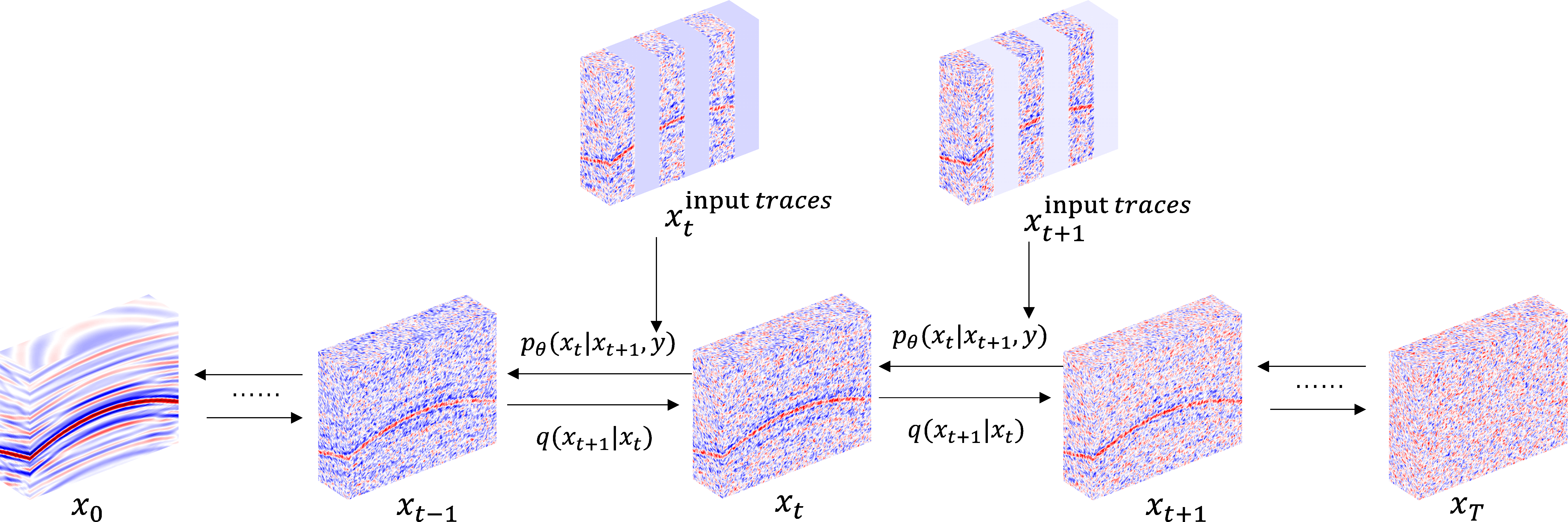
Figure 1: The diffusion model, where $q$ represents the forward encoding training process, and $p$ represents the reverse sampling generation process.

Diffusion models[33], a type of generative model, have recently garnered significant attention for their remarkable success[34]. Unlike convolutional neural networks, diffusion models learn the probability distribution of target data[35], offering desirable attributes such as comprehensive distribution coverage, fixed training objectives, and scalability [36]. Consequently, diffusion models exhibit superior generative performance[37]. As seismic data reconstruction transitions from 2D to 3D, the data’s complexity increases exponentially. The distribution coverage feature of diffusion models enables them to comprehensively capture the distribution of 3D seismic data, resulting in enhanced performance. Therefore, diffusion models prove more adept for 3D seismic data reconstruction tasks. Nonetheless, direct utilization of diffusion models for 3D reconstruction poses challenges. Primarily, diffusion models are unconditional generative models[38], capable of sampling and generating data resembling the probability distribution of the training set without constraints on the generated outcomes. Consequently, utilizing diffusion models directly for reconstruction may yield reconstructed results conflicting with the input data, which is undesirable for reconstruction tasks. Moreover, existing diffusion models designed for image generation are 2D generative models[39] lacking 3D generative capabilities. To address these issues and adapt diffusion models for 3D seismic data reconstruction, we introduce a 3D constrained diffusion model with input guidance (SeisFusion). By learning the probability distribution of seismic data and utilizing input data to guide and constrain the sampling process, SeisFusion effectively accomplishes reconstruction tasks, demonstrating superior reconstruction accuracy in model experiments compared to existing methods. The contributions of this paper are outlined below:

1. Introduced conditional supervision constraints into the diffusion model, constraining the generated data of the diffusion model based on input conditions.

2. Introduced a 3D neural network architecture into the diffusion model, successfully extending the 2D diffusion model to 3D space, and introduced a diffusion model-based reconstruction model (SeisFusion), into 3D seismic data reconstruction work.

3. Improved the model’s generation and reconstruction process by guiding the model to generate reconstructed data through inputting the missing data to be reconstructed into the generation and reconstruction process, resulting in the generation of reconstructed data with higher consistency.

II Diffusion model

Diffusion models, currently the most advanced generative models[40], acquire the probability distribution of data via the forward encoding process. Following training, the data is decoded iteratively from the latent space through the reverse generation process until the target data is attained.

II-A Forward Encoding Training Process:

The forward encoding process gradually encodes samples from the real space to the Tth latent space[41], ultimately transforming them into isotropic Gaussian noise[42]. Given complete seismic data $x_{0}\sim q(x_{0})$ the forward encoding process encodes it into Gaussian noise $x_{T}\sim\mathcal{N}(0,\mathbf{I})$ over T time steps[43]. This process forms a Markov chain[44] determined using a predefined variance table. The encoding process from step t-1 to t can be defined as:

$$q(x_{t}\mid x_{t-1})=\mathcal{N}(\mu_{t},\beta_{t}\mathbf{I})$$ (1)

Where $\beta_{t}$ is obtained from the existing variance table, typically set to linearly increase from 0.0001 to 0.002. $\mu_{t}$ is the mean, according to Nichol et al.[36], $\mu_{t}=\sqrt{1-\beta_{t}}x_{t-1}$. Therefore, Equation (1) can be rewritten as:

$$q(x_{t}\mid x_{t-1})=\mathcal{N}(\sqrt{1-\beta_{t}}x_{t-1},\beta_{t}\mathbf{I})$$ (2)

According to Ho et al.[45], Equation (2) can be further derived to obtain the encoding formula (3) from step 0 to step t:

$$q(x_{t}\mid x_{0})=\mathcal{N}(\sqrt{\overline{\alpha}_{t}}x_{0},(1-\overline{\alpha}_{t})\mathbf{I})$$ (3)

At the same time, $x_{t}$ can be obtained using reparameterization [46].

$$x_{t}=\sqrt{\overline{\alpha}_{t}}x_{0}+\epsilon_{t}\sqrt{(1-\overline{\alpha}_{t})},\epsilon_{t}\sim\mathcal{N}(0,\mathbf{I})$$ (4)

where $\alpha_{t}=1-\beta_{t},\overline{\alpha}_{t}=\prod_{s=0}^{t}\alpha_{s}$. $\epsilon_{t}$ is sampled from a Gaussian distribution.

The diffusion model employs neural networks to model predictions and reverse this encoding process, aiming to obtain the probability distribution $p_{\theta}(x_{t-1}\mid x_{t})$ of the data at step t-1, as shown in Equation (5), where the mean $\mu_{\theta}(x_{t},t)$ and variance $\beta_{\theta}(x_{t},t)$ are obtained from neural networks.

$$p_{\theta}(x_{t-1}\mid x_{t})=\mathcal{N}(\mu_{\theta}(x_{t},t),\beta_{\theta}(x_{t},t))$$ (5)

According to Ho et al.[45] $\mu_{\theta}(x_{t},t)$ can be represented as:

$$\mu_{\theta}(x_{t},t)=\frac{1}{\sqrt{\alpha_{t}}}(x_{t}-\frac{\beta_{t}}{\sqrt{1-\overline{\alpha}_{t}}}\epsilon_{\theta}(x_{t},t))$$ (6)

$\beta_{\theta}(x_{t},t)$ can be represented as:

$$\beta_{\theta}(x_{t},t)=\exp(\epsilon_{\theta}(x_{t},t)\log\beta_{t}+(1-\epsilon_{\theta}(x_{t},t))\log\tilde{\beta_{t}})$$ (7)

Where $\tilde{\beta_{t}}=\frac{1-\overline{\alpha}_{t-1}}{1-\overline{\alpha}_{t}}\beta_{t}$. $\epsilon_{\theta}(x_{t},t)$is the value predicted by the network.

By minimizing the variational lower bound[44] of the negative log-likelihood, we can obtain the loss function of the network:

$$L_{vlb} =\mathbb{E}_{q}[\underbrace{D_{KL}(q(x_{T}\mid x_{0})\parallel p(x_{T}))}_{L_{T}}$$ (8)

$$+\sum_{t>1}\underbrace{D_{KL}(q(x_{t}\mid x_{t-1},x_{0})\parallel p_{\theta}(x_{t-1}\mid x_{t}))}_{L_{t-1}}$$

$$-\underbrace{\log p_{\theta}(x_{0}\mid x_{1})}_{L_{0}}]$$

Where $D_{KL}$ is the KL divergence, which describes the loss between the encoding distribution q and the network generated decoding distribution p.

According to Ho et al.[45], during single step training, only the $L_{t-1}$ loss needs to be computed. Hence, a simplified loss function can be derived as shown in Equation (9), where $\epsilon_{t}$ is given by Equation (4).

$$L_{simple}=E_{t,x_{0},\epsilon_{t}}[\lVert\epsilon_{t}-\epsilon_{\theta}(x_{t},t)\rVert^{2}]$$ (9)

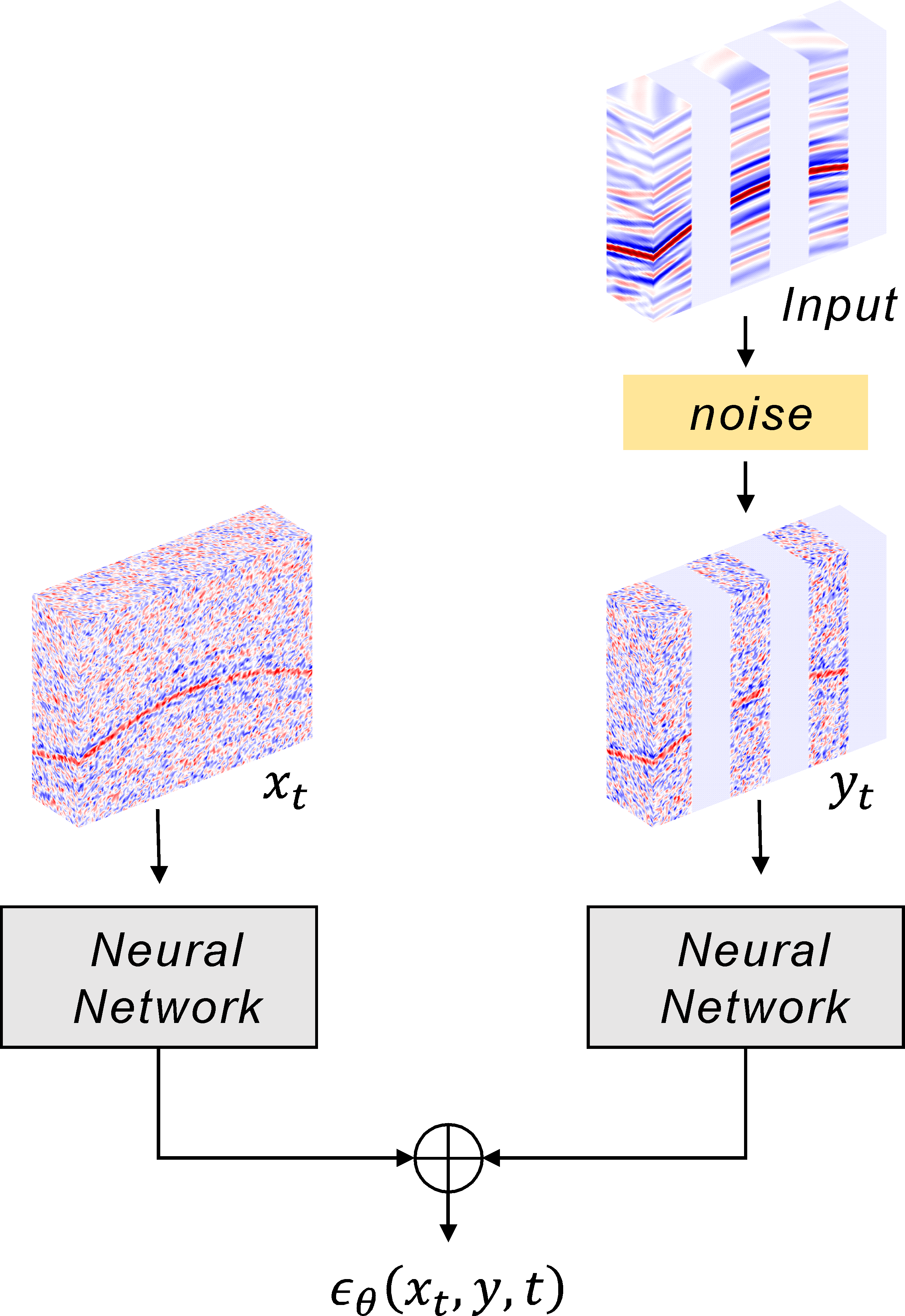
Figure 2: Overall framework of the noise matching network.

II-B Reverse sampling generation process:

After training, the diffusion model starts decoding the data from the latent space iteratively until it reaches the target data, as shown in Fig. 1. The decoding process from step t to step t-1 is as follows:

$$p_{\theta}(x_{t-1}\mid x_{t})=\mathcal{N}(\mu_{\theta}(x_{t},t),\beta_{\theta}(x_{t},t))$$ (10)

Using equations (6) and (7), the reparameterization technique can be employed to obtain $x_{t-1}$.

$$x_{t-1} =\frac{1}{\sqrt{\alpha_{t}}}(x_{t}-\frac{\beta_{t}}{\sqrt{1-\overline{\alpha}_{t}}}\epsilon_{\theta}(x_{t},t))$$ (11)

$$+\epsilon\sqrt{\exp(\epsilon_{\theta}(x_{t},t)\log\beta_{t}+(1-\epsilon_{\theta}(x_{t},t))\log\tilde{\beta_{t}})},\epsilon\sim\mathcal{N}(0,\mathbf{I})$$

Iterative sampling continues until obtaining the pure target data $x_{0}$

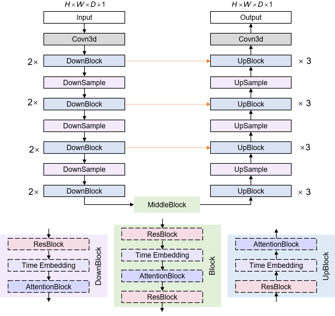
Figure 3: Backbone network architecture.

III Method

III-A Constraint correction:

The diffusion model functions as a purely unconditional generative model. Following training, it can sample and generate data possessing a probability distribution akin to the training set. However, the entire sampling process remains unconstrained, potentially yielding diverse outcomes when sampling commences from distinct latent variables, albeit some may exhibit high consistency with the data intended for reconstruction. Hence, we aim to incorporate supervised constraints into the diffusion model. These constraints endeavor to align $x_{t-1}$, sampled at step $t$, with the (t-1)th latent space vector encoded by the ground truth. After undergoing T constraints, even when starting from different latent variables, the final sampling results will approximate the true values. The forward encoding process and the reverse sampling generation process with constraints are illustrated in Fig. 1.

In the forward encoding training process, after introducing self-supervised constraints, Equation (5) is rewritten as:

$$p_{\theta}(x_{t-1}\mid x_{t})=\mathcal{N}(\mu_{\theta}(x_{t},y,t),\beta_{\theta}(x_{t},y,t))$$ (12)

$\mu_{\theta}(x_{t},y,t)$ is represented as:

$$\mu_{\theta}(x_{t},y,t)=\frac{1}{\sqrt{\alpha_{t}}}(x_{t}-\frac{\beta_{t}}{\sqrt{1-\overline{\alpha}_{t}}}\epsilon_{\theta}(x_{t},y,t))$$ (13)

$\beta_{\theta}(x_{t},y,t)$ is represented as:

$$\beta_{\theta}(x_{t},y,t)=\exp(\epsilon_{\theta}(x_{t},y,t)\log\beta_{t}+(1-\epsilon_{\theta}(x_{t},y,t))\log\tilde{\beta_{t}})$$ (14)

Where $\tilde{\beta_{t}}=\frac{1-\overline{\alpha}_{t-1}}{1-\overline{\alpha}_{t}}\beta_{t}$. The network is modified to estimate $\epsilon_{\theta}(x_{t},y,t)$. The value of $y$ is the self-supervised constraint we introduce into the constrained diffusion model.

After introducing self-supervised constraints, the loss function derived from the variational lower bound considerations is rewritten as:

$$L_{vlb} =\mathbb{E}_{q}[\underbrace{D_{KL}(q(x_{T}\mid x_{0})\parallel p(x_{T}))}_{L_{T}}$$ (15)

$$+\sum_{t>1}\underbrace{D_{KL}(q(x_{t}\mid x_{t-1,x_{0}})\parallel p_{\theta}(x_{t-1}\mid x_{t},y))}$$

$${}_{L_{t-1}}-\underbrace{\log p_{\theta}(x_{0}\mid x_{1},y)}_{L_{0}}]$$

The simplified loss function derived from $L_{t-1}$ is rewritten as:

$$L_{simple}=E_{t,x_{0},\epsilon_{t}}[\lVert\epsilon_{t}-\epsilon_{\theta}(x_{t},y,t)\rVert^{2}]$$ (16)

In the reverse sampling generation process, after introducing self-supervised constraints, the sampling at step t is:

$$p_{\theta}(x_{t-1}\mid x_{t})=\mathcal{N}(\mu_{\theta}(x_{t},y,t),\beta_{\theta}(x_{t},y,t))$$ (17)

Using equations (13) and (14), we can obtain $x_{t-1}$ using the reparameterization technique:

$$x_{t-1} =\frac{1}{\sqrt{\alpha_{t}}}(x_{t}-\frac{\beta_{t}}{\sqrt{1-\overline{\alpha}_{t}}}\epsilon_{\theta}(x_{t},y,t))$$ (18)

$$+\epsilon\sqrt{\exp(\epsilon_{\theta}(x_{t},y,t)\log\beta_{t}+(1-\epsilon_{\theta}(x_{t},y,t))\log\tilde{\beta_{t}})},\epsilon\sim\mathcal{N}(0,\mathbf{I})$$

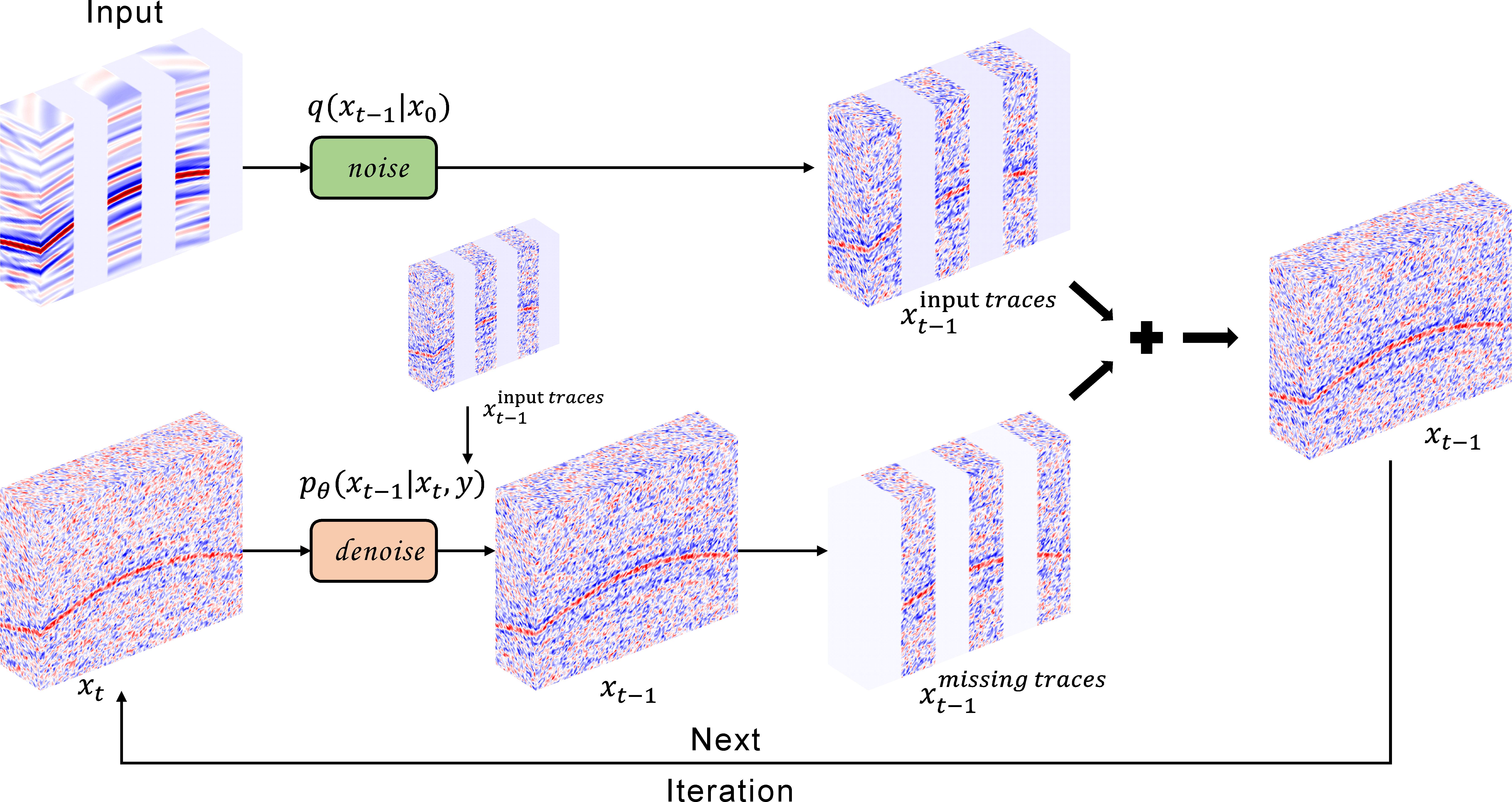
Figure 4: Guided sampling.

III-B 3D neural network architecture:

In the diffusion model, neural networks are employed to estimate the noise scale, denoted as $\epsilon_{\theta}(x_{t},y,t)$ in Equation (18). The precision in estimating $\epsilon_{\theta}(x_{t},y,t)$ corresponding to the current step t directly impacts the quality of the generated data. Hence, extending the diffusion model from 2D to 3D preserves its original forward encoding training and reverse sampling generation principles. Consequently, its forward encoding process remains a fixed Markov chain, as depicted in Fig. 1. Although the training objective still adheres to Equation (16), adjustments in the neural network architecture for generating $\epsilon_{\theta}(x_{t},y,t)$ are necessary to render it suitable for 3D tasks.

To tailor the diffusion model for 3D generation tasks, we introduce a 3D architecture with conditional constraints. The comprehensive architecture is outlined in Fig. 2

The network’s prediction of $\epsilon_{\theta}(x_{t},y,t)$ comprises two components: one entails the conditional features derived from the backbone network’s output. The input to the backbone network, $y_{t}$, is obtained through the encoding of known traces. The other component involves input $x_{t}$ into the backbone network, which yields encoded features. Subsequently, these two components are fused to derive $\epsilon_{\theta}(x_{t},y,t)$. The feature fused $\epsilon_{\theta}(x_{t},y,t)$ is then constrained by the input known data.

The overall structure of the backbone network is shown in Fig. 3, which is a 3D UNet with attention and time embedding. The encoding part of the UNet consists of DownBlocks and DownSamples, where DownBlock deepens the channel without changing the size of the feature map. The decoding part of the UNet comprises UpBlocks and UpSamples, ensuring that the output and input maintain the same size dimensions. Each DownBlock and UpBlock performs time embedding to embed the information of the current step $t$, allowing the network to learn the information of $t$ to the fullest extent and enabling more precise prediction of the encoded features and conditional features by the network.

Figure 5: Dataset, left is SEG C3, Right is Mobil Avo Viking Graben Line 12.

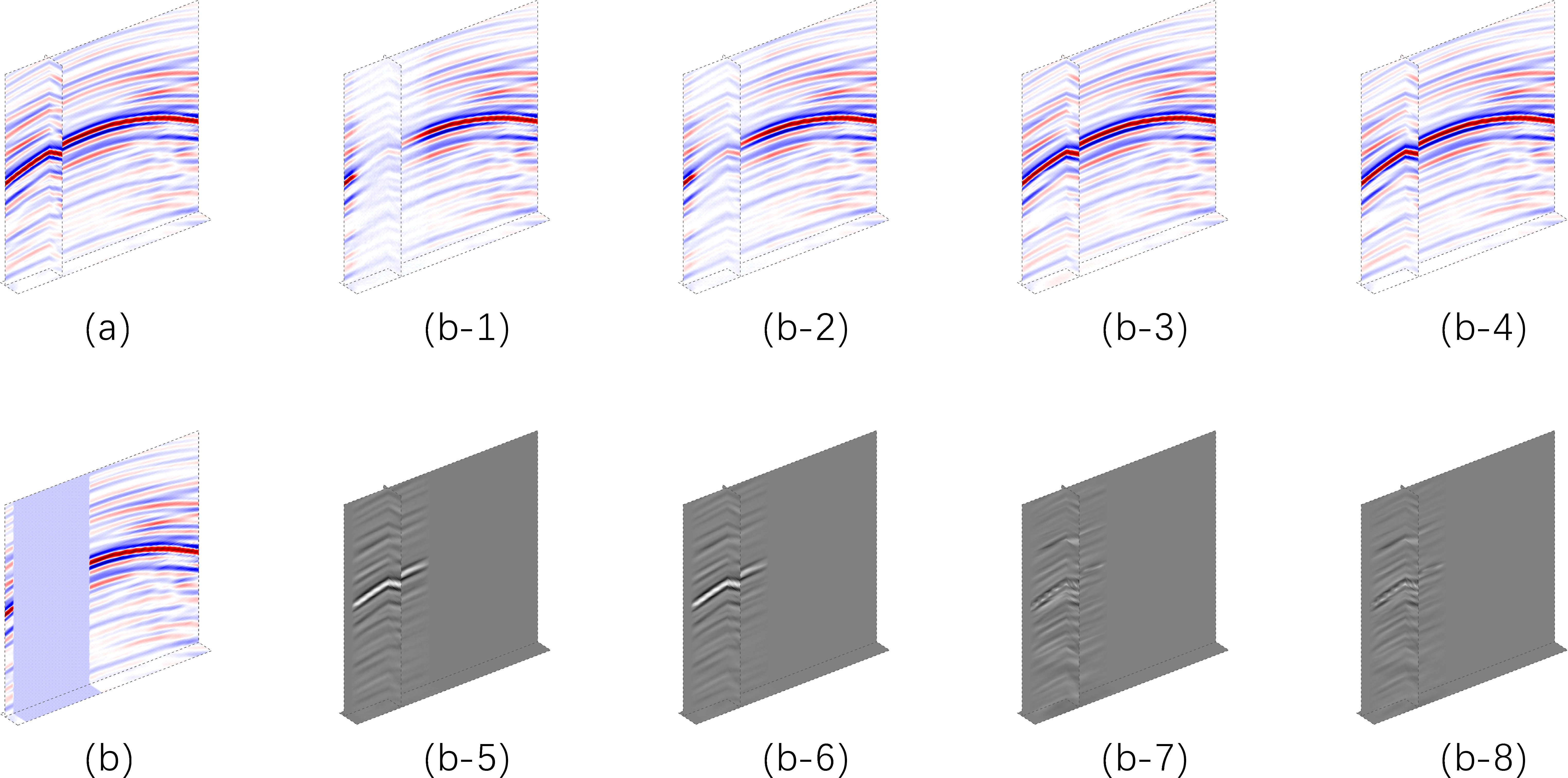
Figure 6: (a) Ground truth, (b) 50% 50 continuous missing traces, (b-1)-(b-4) are the reconstruction results with u-values set to 1, 5, 10, and 15, respectively, and (b-5)-(b-8) are the residuals of each reconstruction result relative to Ground truth, respectively.

III-C Guided sampling

The diffusion model described in Section II is an unconditional generative model. It iteratively decodes samples from the $T$th latent space until the target data is obtained. This sampling process does not accept any prior information. Therefore, directly using the diffusion model for seismic data reconstruction leads to conflicts between the probability distribution of the generated data and that of the data to be reconstructed. Consequently, the reconstruction results struggle to maintain high consistency with the data to be reconstructed, which is undesirable for data reconstruction tasks. The guided sampling approach we propose effectively addresses this issue.

When the diffusion model samples $x_{t-1}$ from $x_{t}$, if $x_{t}$ contains prior information about known data, then the generated $x_{t-1}$ naturally includes the prior information of the known data[47]. As a result, the iteratively sampled $x_{0}$ will exhibit better consistency with the known data. In guided sampling, we represent seismic data as $x$, where the known portion is denoted as $(1-m)\odot x$ and the portion to be reconstructed is denoted as $m\odot x$. Then make the following improvement in sampling $x_{t-1}$ from $x_{t}$:

$$x_{t-1}^{known}\sim\mathcal{N}(\sqrt{\overline{\alpha}_{t-1}}x_{0},(1-\overline{\alpha}_{t-1})\mathbf{I})$$ (19a)

$$x_{t-1}^{unknown}\sim\mathcal{N}(\mu_{\theta}(x_{t},y,t),\beta_{\theta}(x_{t},y,t)\mathbf{I})$$ (19b)

$$x_{t-1}=(1-m)\odot x_{t-1}^{known}+m\odot x_{t-1}^{unknown}$$ (19c)

Thus, $x_{t-1}$ consists of two parts: one part is encoded from the known data to the ${t-1}$ latent space through the forward encoding process, and the other part is sampled from $x_{t}$ during the sampling process. At this point, $x_{t-1}$ contains the prior information of the known data. However, $x_{t-1}$ still lacks consistency with the known data, and continuing to sample $x_{t-2}$ will not resolve this conflict. However, we can encode $x_{t-1}$ back into $x_{t}$ and obtain $x_{t-1}$ again using the above method. In this case, $x_{t-1}$ will have higher consistency. We repeat this process, and the resulting $x_{t-1}$ will no longer have consistency conflicts. The overall process is illustrated in Fig. 4, and specific steps are listed in Algorithm 1.

Algorithm 1 Seismic data reconstruction algorithm.

  

   for $t=T,\ldots,1$

        for $u=1,\ldots,U$

           $\epsilon\sim\mathcal{N}(0,I)$ if $t>1$,else $\epsilon=0$

           $x_{t-1}^{known}=\sqrt{\overline{\alpha}_{t}}x_{0}+\epsilon\sqrt{(1-\overline{\alpha}_{t})})$

           $z\sim\mathcal{N}(0,I)$ if $t>1$,else $z=0$

           $x_{t-1}^{unknown}=\frac{1}{\sqrt{\alpha_{t}}}(x_{t}-\frac{\beta_{t}}{\sqrt{1-\overline{\alpha}_{t}}}\epsilon_{\theta}(x_{t},y,t))+z\sigma_{t}$

           $x_{t-1}=(1-m)\odot x_{t-1}^{known}+m\odot x_{t-1}^{unknown}$

            if $u<U$ and $t>1$ then

               $x_{t}\sim\mathcal{N}(\sqrt{1-\beta_{t-1}}x_{t-1},\beta_{t-1}\mathbf{I})$

            end if

        end for

   end for

   return $x_{0}$

IV Experiments

IV-A Evaluation Metrics:

To quantitatively evaluate the quality of the reconstruction results, we selected three commonly used metrics, namely MSE, SNR, and SSIM. MSE measures the error between the reconstruction result and the ground truth, calculated using the following formula:

$$MSE=\frac{1}{n}\sum_{i=1}^{n}(x_{i}^{r}-x_{i}^{t})^{2}$$ (20)

Where $x_{i}^{r}$ represents the data reconstructed by the network, $x_{i}^{t}$ represents the ground truth, and the closer the MSE value is to 0, the closer the reconstruction result is to the ground truth. SNR measures the quality of the reconstruction result, calculated by the following formula:

$$SNR=10log_{10}\frac{\parallel x_{r}\parallel_{F}^{2}}{\parallel x_{t}-x_{r}\parallel_{F}^{2}}$$ (21)

Where $x_{r}$ represents the data reconstructed by the network, $x_{t}$ represents the ground truth, $\parallel\parallel$ denotes the Frobenius norm, and the higher the SNR value, the higher the quality of the reconstruction result. SSIM measures the structural similarity of the reconstruction result, calculated by the following formula:

$$SSIM=\frac{(2\mu_{r}\mu_{t}+c_{1})(2\sigma_{rt}+c_{2})}{(\mu_{r}^{2}\mu_{t}^{2}+c_{1})(\sigma_{r}^{2}+\sigma_{t}^{2}+c_{2})}$$ (22)

Where $\mu_{r}$ is the mean of the reconstructed result, $\mu_{t}$ is the mean of the ground truth, $2\sigma_{rt}$ is the covariance between the reconstructed result and the ground truth, $\sigma_{r}$ is the variance of the reconstructed result, $\sigma_{t}$ is the variance of the ground truth, and $c_{1}$ and $c_{2}$ are two constants introduced to avoid numerical instability. The SSIM value closer to 1 indicates that the reconstruction result is closer to the ground truth.

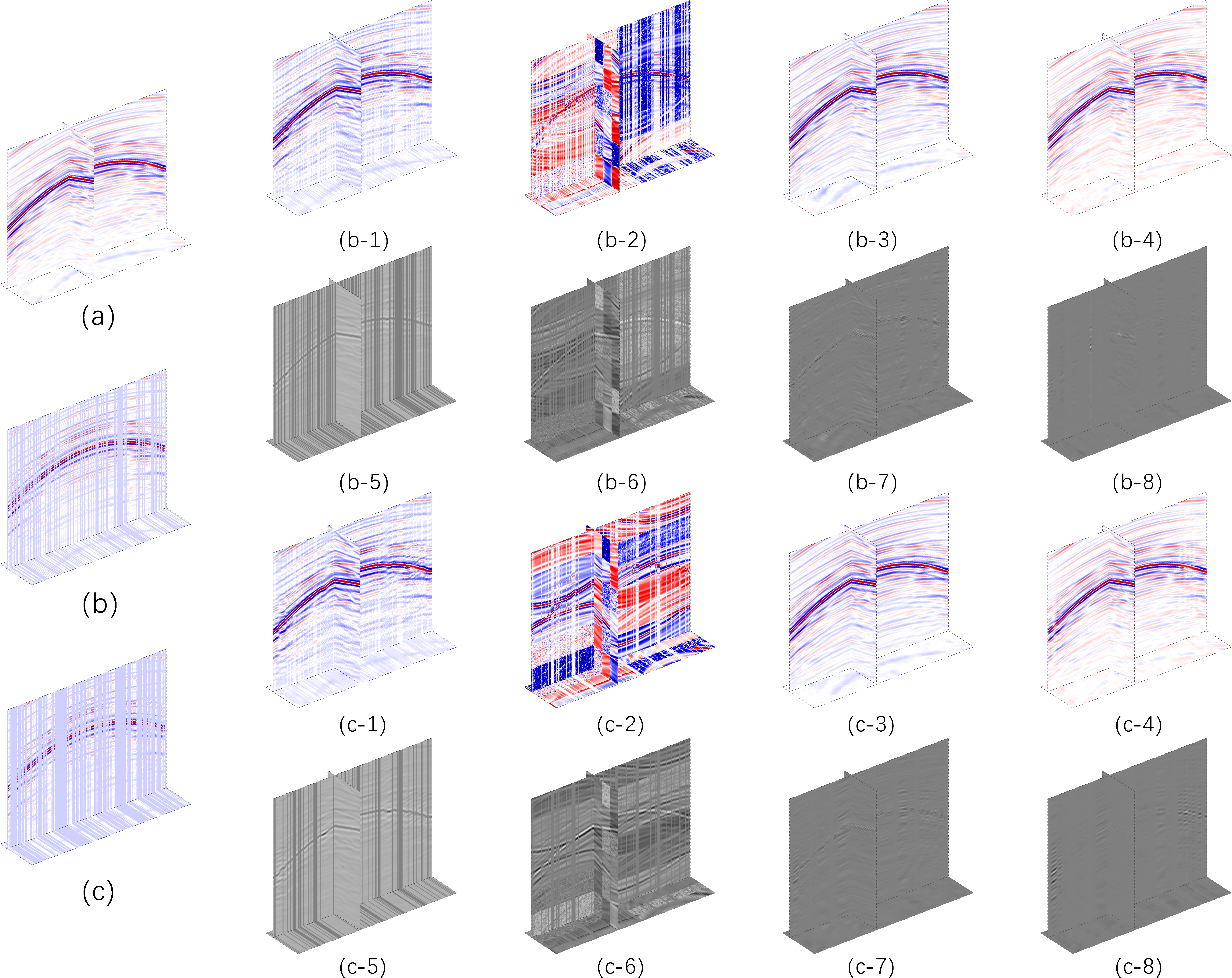
Figure 7: (a) Ground truth,(b) 50% random missing, (b-1) to (b-4) are the reconstruction results of Unet, diffusion model, MDA GAN, and SeisFusion, respectively. (b-5) to (b-8) are the residuals of each reconstruction result relative to the ground truth.(c) 80% random missing, (c-1) to (c-4) are the reconstruction results of Unet, diffusion model, MDA GAN, and SeisFusion, respectively. (c-5) to (c-8) are the residuals of each reconstruction result relative to the ground truth.

IV-B Train:

Our experiments were conducted on two datasets as shown in Fig. 5, the publicly available synthetic dataset SEG C3 and the field dataset Mobil Avo Viking Graben Line 12. We divided the datasets into three parts: 3/5 for training, 1/5 for validation, and 1/5 for testing. The patch size was set to 16x32x128. Randomly missing training samples were used as constraint inputs. We set T, the number of iterations in the forward process, to 1000. Adam was chosen as the optimization algorithm with a learning rate of 1e-5. The models were trained for 500,000 steps on two RTX3090Ti GPUs, and the model with the lowest loss on the validation set was selected as the final model for testing.

IV-C Ablation:

In order to reasonably determine the values for the parameter $u$ in Algorithm 1, we first conducted ablation studies. The ablation studies were conducted on a patch of size 16×128×128 from the SEG C3 dataset, where 50% of contiguous traces were set to 0 to represent missing traces. Different values of $u$ were set for reconstruction, and the results are shown in Fig. 6.

When the value of $u$ is set to 1, no iterative guided sampling is performed. The reconstruction result is generated by a constrained diffusion model without guided sampling constraints. It can be observed that the generated results at this point no longer exhibit randomness and have been constrained to a reasonable range, although the generation details still need improvement. As the value of $u$ increases to 5, the reconstruction details noticeably improve. Further increasing $u$ to 10, the reconstruction quality reaches a bottleneck, showing higher consistency with the ground truth. We computed evaluation metrics for four values of $u$ as shown in Table I to quantitatively assess the influence of $u$ on the reconstruction results. It can be seen that as $u$ increases, the reconstruction performance gradually improves, reaching a bottleneck at $u=10$. Increasing $u$ further does not significantly enhance the reconstruction quality. Therefore, setting $u$ to 10 is a reasonable choice.

TABLE I: Ablation study.

U	MSE	SNR	SSIM
1	1.7282e-3	27.6239	0.9196
2	1.1313e-3	29.4639	0.9510
10	1.6460e-4	37.8356	0.9875
15	1.7072e-4	37.6770	0.9880

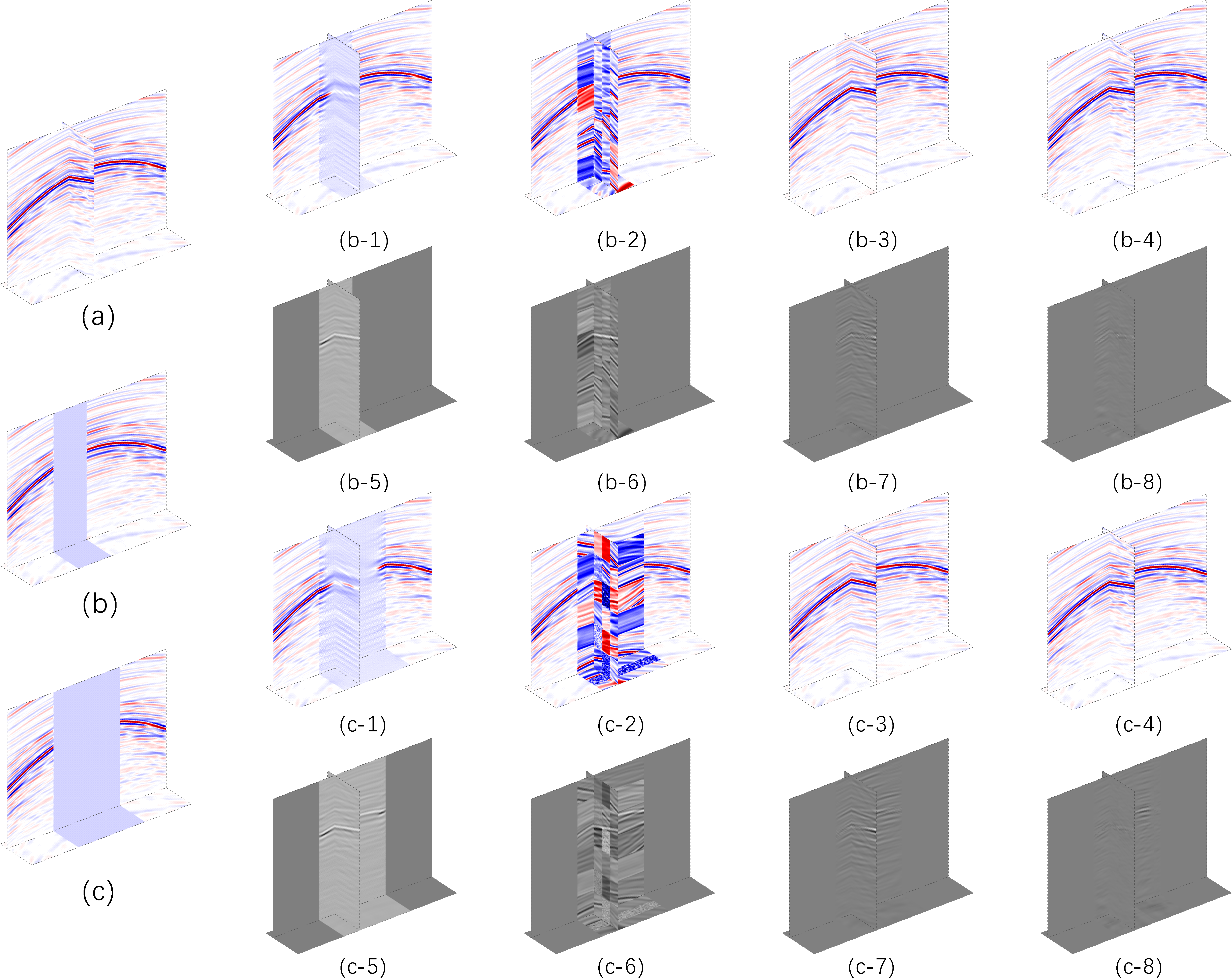
Figure 8: (a) Ground truth,(b) 50 continuous missing traces, (b-1) to (b-4) are the reconstruction results of Unet, diffusion model, MDA GAN, and SeisFusion, respectively. (b-5) to (b-8) are the residuals of each reconstruction result relative to the ground truth.(c) 100 continuous missing traces, (c-1) to (c-4) are the reconstruction results of Unet, diffusion model, MDA GAN, and SeisFusion, respectively. (c-5) to (c-8) are the residuals of each reconstruction result relative to the ground truth.

IV-D Data Reconstruction:

During the sampling generation process, in Algorithm 1, T is set to 250 based on the state-of-the-art diffusion model, and u is set to 10. To validate the effectiveness of our proposed method, we selected three other models for comparative testing: Unet, diffusion model, and MDA GAN. Unet is the most commonly used model, which has been proven to have excellent performance in seismic data reconstruction[23]. The diffusion model[45] is directly extended from the 2D model, with training parameters consistent with our model. For MDA GAN[16], the authors provided the source code and weight files, stating that they did not need to be retrained. Therefore, we directly used the code and weights provided by the authors for reconstruction without any modifications.

IV-D1 SEG C3

To validate the effectiveness of our method, we first conducted tests on the synthetic dataset SEG C3. To fully evaluate the reconstruction performance of the proposed method under different missing scenarios, we divided the tests into two parts: random discrete missing and continuous missing.

Random discrete missing: To simulate possible complex situations, we set two different missing rates, 50% and 80%, by setting traces to 0 to represent missing data. Fig. 7 shows the reconstruction results of different methods under these two missing rates. It can be observed that the reconstruction results of Unet already show low consistency at a 50% missing rate, and the discontinuity becomes more pronounced when the missing rate increases to 80%. Residual plots indicate a significant deviation between its reconstruction results and ground truth. The original diffusion model, lacking constraints and subject to sampling uncertainty, yields highly random and deviant reconstruction results compared to the ground truth. Both MDA GAN and our method perform well in reconstructing data under both missing scenarios, with a slight advantage of our method over MDA GAN, as indicated by residual plots.

To quantitatively evaluate the reconstruction performance of the four models, we computed four evaluation metrics, as shown in Table II. It can be seen that our method achieves the best results under different missing rates, with a significant lead in both MSE and SNR metrics.

TABLE II: Comparison of four reconstruction networks under random missing on synthetic dataset.

		MSE	SNR	SSIM
Random Missing 50% Traces	UNet	1.4964e-4	34.1305	0.9613
	Diffusion Model	1.3898e-3	25.3783	0.8751
	MDA GAN	1.2719e-4	38.5153	0.9823
	SeisFusion	2.3166e-5	46.3513	0.9987
Random Missing 80% Traces	UNet	1.7086e-3	30.7259	0.9326
	Diffusion Model	5.1474e-3	22.3783	0.8595
	MDA GAN	2.9637	35.2825	0.9789
	SeisFusion	2.27954-4	36.4215	0.9881

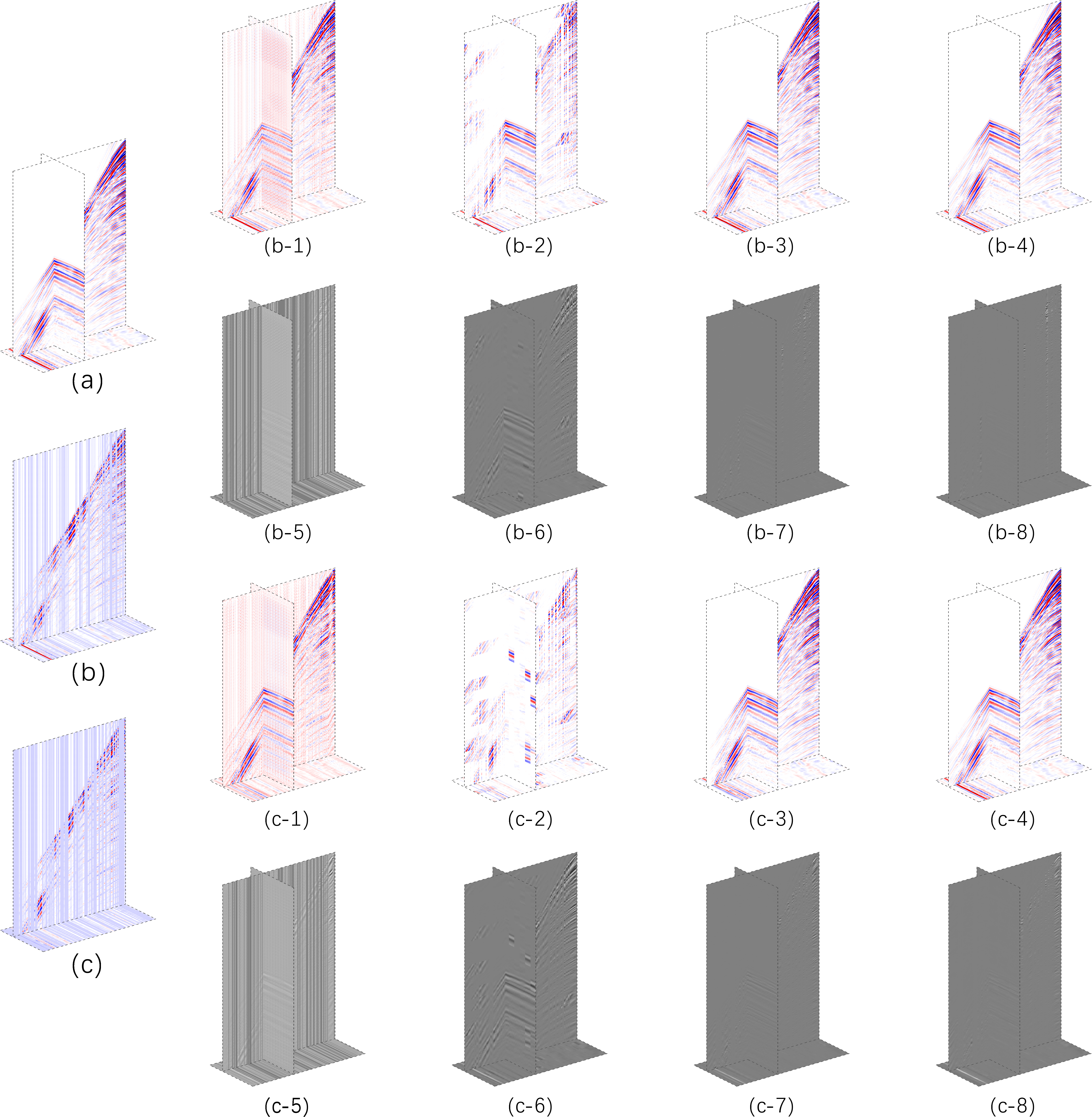
Figure 9: (a) Ground truth,(b) 50% random missing, (b-1) to (b-4) are the reconstruction results of Unet, diffusion model, MDA GAN, and SeisFusion, respectively. (b-5) to (b-8) are the residuals of each reconstruction result relative to the ground truth.(c) 80% random missing, (c-1) to (c-4) are the reconstruction results of Unet, diffusion model, MDA GAN, and SeisFusion, respectively. (c-5) to (c-8) are the residuals of each reconstruction result relative to the ground truth.

Continuous missing: To evaluate the reconstruction performance of the proposed method under continuous missing, we set two scenarios of continuous missing, 50 continuous missing traces and 100 continuous missing traces. Traces were set to 0 to represent missing data. The reconstruction results of the four models are shown in Fig. 8. It can be observed that UNet fails to reconstruct seismic data under continuous missing, showing poor reconstruction performance. The original diffusion model also fails to complete the reconstruction task well due to the lack of constraints and sampling guidance under continuous missing. According to the residual maps, significant deviations from the ground truth can be observed in some areas. MDA GAN achieves relatively good reconstruction results, but deviations and inconsistencies still appear at the missing boundaries. Our method consistently provides the best reconstruction results under different missing scenarios.

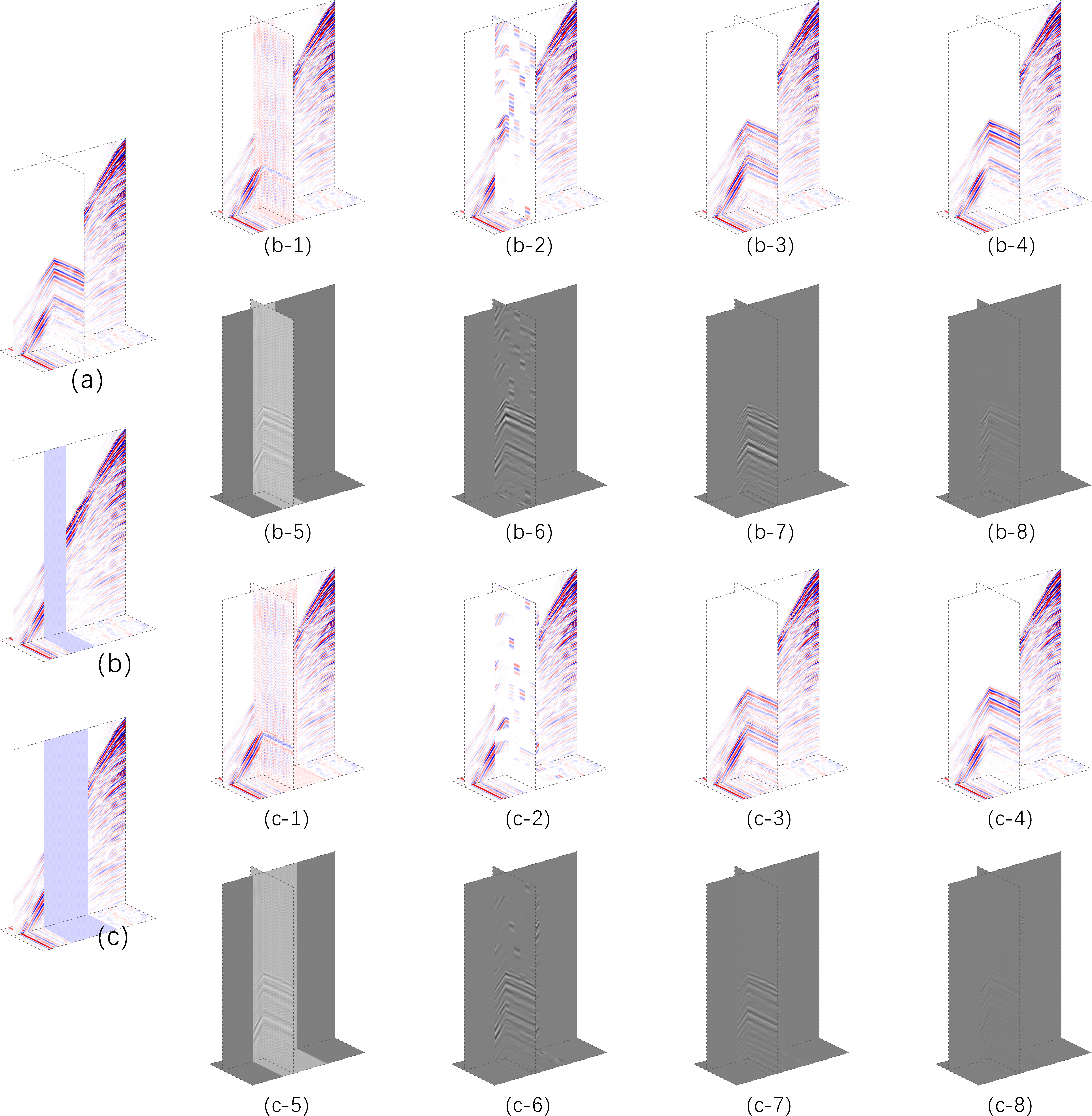
Figure 10: (a) Ground truth,(b) 50 continuous missing traces, (b-1) to (b-4) are the reconstruction results of Unet, diffusion model, MDA GAN, and SeisFusion, respectively. (b-5) to (b-8) are the residuals of each reconstruction result relative to the ground truth.(c) 100 continuous missing traces, (c-1) to (c-4) are the reconstruction results of Unet, diffusion model, MDA GAN, and SeisFusion, respectively. (c-5) to (c-8) are the residuals of each reconstruction result relative to the ground truth..

To quantitatively evaluate the reconstruction performance of the four models, we calculate four evaluation metrics under continuous missing, as shown in Table III. It can be seen that our method achieves the best results under different missing rates, with significant advantages in both MSE and SNR metrics. Especially under 100 continuous missing traces, our method also maintains a significant lead in the SSIM metric.

TABLE III: Comparison of four reconstruction networks under continuous missing on synthetic dataset.

		MSE	SNR	SSIM
50 continuous missing traces	UNet	0.0567	12.4661	0.7579
	Diffusion Model	5.4142e-3	22.6646	0.8432
	MDA GAN	3.5121e-4	34.5442	0.9767
	SeisFusion	1.9208e-5	47.1651	0.9988
100 continuous missing traces	UNet	0.1116	9.5230	0.7095
	Diffusion Model	0.0155	18.0705	0.6844
	MDA GAN	2.0235e-4	26.9389	0.9027
	SeisFusion	6.2141e-5	42.0662	0.9965

IV-D2 Mobil Avo Viking Graben Line 12

In order to further evaluate the performance of the proposed method and validate the effectiveness of the approach, we proceeded with testing on the Mobil Avo Viking Graben Line 12 field dataset. The testing was divided into two parts: random discrete missing and Continuous Missing.

Random discrete missing: we set two different missing rates, 50% and 80%, where traces were set to 0 to represent the missing data. Fig. 9 displays the reconstruction results of different methods under these two missing rates. It can be observed that the reconstruction results of UNet and the original diffusion model already show low consistency at 50% missing rate, and as the missing rate increases, the inconsistency becomes more apparent, as indicated by the residual plots showing significant deviations from the ground truth. Both MDA GAN and our method performed well in reconstructing under both missing scenarios, with our method slightly outperforming MDA GAN according to the residual plots.

To quantitatively evaluate the reconstruction results of the four models, we calculated four evaluation metrics as shown in Table IV. It can be seen that our method achieved the best performance under different missing rates, with a significant lead in both MSE and SNR evaluation

TABLE IV: Comparison of four reconstruction networks under random missing on filed dataset.

		MSE	SNR	SSIM
Random Missing 50% Traces	UNet	5.1437e-3	29.3055	0.9173
	Diffusion Model	5.6712e-3	22.9027	0.8482
	MDA GAN	2.3697e-4	36.2529	0.9900
	SeisFusion	9.1223e-5	40.3989	0.9961
Random Missing 80% Traces	Missing	9.7737e-3	17.5117	0.8597
	Traces	9.8717e-3	21.5047	0.8061
	MDA GAN	5.6353e-4	32.4908	0.9772
	SeisFusion	3.0559e-4	35.1493	0.9891

Continuous missing: we similarly set two scenarios: continuous missing of 50 traces and continuous missing of 100 traces. Traces were set to 0 to represent the missing data, and the reconstruction results of the four models are shown in Fig. 10. It can be observed that UNet fails to reconstruct seismic data under continuous missing, and the original diffusion model, due to lack of constraints and sampling guidance, produces discontinuous and inconsistent data under 50-trace continuous missing, which becomes more pronounced with 100-trace continuous missing. According to the residual plots, significant deviations from the ground truth are observed, particularly at larger missing values. MDA GAN performs relatively well in reconstruction, but deviations and inconsistencies still appear at the missing boundaries. Our method provides optimal reconstruction results under different missing scenarios.

To quantitatively evaluate the reconstruction results of the four models, we calculated four evaluation metrics under continuous missing, as shown in Table V. It can be seen that our method achieves the best performance under different missing rates, with a significant lead in both MSE and SNR evaluation metrics. Particularly, under 100-trace continuous missing, our method also maintains a substantial lead in the SSIM metric.

TABLE V: Comparison of four reconstruction networks under continuous missing on filed dataset.

		MSE	SNR	SSIM
50 continuous missing traces	UNet	0.0505	12.9651	0.7792
	Diffusion Model	6.1376e-3	21.9251	0.8418
	MDA GAN	2.9249e-4	35.3388	0.9774
	SeisFusion	6.4218e-5	41.9234	0.9945
100 continuous missing traces	Missing	0.1012	9.9480	0.5788
	Traces	0.0987	21.6757	0.7321
	MDA GAN	1.1688e-3	29.3224	0.9390
	SeisFusion	3.0648e-4	35.1359	0.9848

The experiments on synthetic and filed datasets indicate that as the complexity of missing traces increases, the reconstruction performance experiences varying degrees of decline. This is largely because when the seismic data reconstruction task extends from 2D to 3D, the diversity of data exhibits exponential growth, whereas convolutional neural networks performing point-to-point reconstruction cannot achieve comprehensive distribution coverage. Therefore, with increasing complexity of missing traces, particularly in reconstructing continuous large missing segments, the performance degradation becomes more pronounced. In contrast, the diffusion model learns the probability distribution of the target data and can provide ideal characteristics of distribution coverage. Thus, our method maintains relatively good reconstruction accuracy when facing complex missing scenarios, especially continuous large missing segments.

V Conclusions

This paper proposes a 3D diffusion model with guided sampling and constraint incorporation for reconstructing complex 3D seismic data. Guided sampling utilizes input seismic data to guide the generation of reconstructed data by sampling from the given data during the sampling generation process. By incorporating constraints, uncertainties produced by the diffusion model’s sampling process are successfully avoided, marking the first successful application of the diffusion model to 3D seismic data reconstruction. This method reconstructs data by learning the distribution of existing seismic data, effectively avoiding the performance degradation of traditional convolutional networks when faced the data to be reconstructed exhibits complex missing patterns, due to point-to-point learning reconstruction. Some ablation studies were conducted to validate the rationality of the hyperparameter settings used in the proposed method. Comparative experimental results on synthetic and filed datasets demonstrate that our proposed method yields more accurate interpolation results compared to other existing methods. The diffusion model itself, by learning the data distribution, possesses higher generative accuracy and generalization capability, allowing our network to generalize to more complex missing scenarios during inference.

References

- [1] R. Dai, C. Yin, S. Yang, and F. Zhang, “Seismic deconvolution and inversion with erratic data,” Geophysical Prospecting, vol. 66, no. 9, pp. 1684–1701, 2018.
- [2] Y. Chen, X. Chen, Y. Wang, and S. Zu, “The interpolation of sparse geophysical data,” Surveys in Geophysics, vol. 40, pp. 73–105, 2019.
- [3] M. J. Porsani, “Seismic trace interpolation using half-step prediction filters,” Geophysics, vol. 64, no. 5, pp. 1461–1467, 1999.
- [4] N. Gülünay, “Seismic trace interpolation in the fourier transform domain,” Geophysics, vol. 68, no. 1, pp. 355–369, 2003.
- [5] B. Wang, N. Zhang, W. Lu, and J. Wang, “Deep-learning-based seismic data interpolation: A preliminary result,” Geophysics, vol. 84, no. 1, pp. V11–V20, 2019.
- [6] S. Fomel, “Seismic reflection data interpolation with differential offset and shot continuation,” Geophysics, vol. 68, no. 2, pp. 733–744, 2003.
- [7] J. Ronen, “Wave-equation trace interpolation,” Geophysics, vol. 52, no. 7, pp. 973–984, 1987.
- [8] A. Latif and W. A. Mousa, “An efficient undersampled high-resolution radon transform for exploration seismic data processing,” IEEE Transactions on Geoscience and Remote Sensing, vol. 55, no. 2, pp. 1010–1024, 2016.
- [9] J. Wang, M. Ng, and M. Perz, “Seismic data interpolation by greedy local radon transform,” Geophysics, vol. 75, no. 6, pp. WB225–WB234, 2010.
- [10] X. Niu, L. Fu, W. Zhang, and Y. Li, “Seismic data interpolation based on simultaneously sparse and low-rank matrix recovery,” IEEE Transactions on Geoscience and Remote Sensing, vol. 60, pp. 1–13, 2021.
- [11] W. Zhang, L. Fu, and Q. Liu, “Nonconvex log-sum function-based majorization–minimization framework for seismic data reconstruction,” IEEE Geoscience and Remote Sensing Letters, vol. 16, no. 11, pp. 1776–1780, 2019.
- [12] Y. A. S. Innocent Oboué, W. Chen, H. Wang, and Y. Chen, “Robust damped rank-reduction method for simultaneous denoising and reconstruction of 5d seismic data,” Geophysics, vol. 86, no. 1, pp. V71–V89, 2021.
- [13] Y. Zhou and C. Han, “Seismic data restoration based on the grassmannian rank-one update subspace estimation method,” Journal of Applied Geophysics, vol. 159, pp. 731–741, 2018.
- [14] Y. Wang, B. Wang, N. Tu, and J. Geng, “Seismic trace interpolation for irregularly spatial sampled data using convolutional autoencoder,” Geophysics, vol. 85, no. 2, pp. V119–V130, 2020.
- [15] J. Park, D. Yoon, S. J. Seol, and J. Byun, “Reconstruction of seismic field data with convolutional u-net considering the optimal training input data,” in SEG International Exposition and Annual Meeting. SEG, 2019, p. D023S027R005.
- [16] Y. Dou, K. Li, H. Duan, T. Li, L. Dong, and Z. Huang, “Mda gan: Adversarial-learning-based 3-d seismic data interpolation and reconstruction for complex missing,” IEEE Transactions on Geoscience and Remote Sensing, vol. 61, pp. 1–14, 2023.
- [17] M. M. Abedi and D. Pardo, “A multidirectional deep neural network for self-supervised reconstruction of seismic data,” IEEE Transactions on Geoscience and Remote Sensing, vol. 60, pp. 1–9, 2022.
- [18] O. M. Saad, S. Fomel, R. Abma, and Y. Chen, “Unsupervised deep learning for 3d interpolation of highly incomplete data,” Geophysics, vol. 88, no. 1, pp. WA189–WA200, 2023.
- [19] H. Wang, J. Zhang, Z. Zhao, C. Zhang, L. Long, Z. Yang, and W. Geng, “Automatic velocity picking using a multi-information fusion deep semantic segmentation network,” IEEE Transactions on Geoscience and Remote Sensing, vol. 60, pp. 1–10, 2022.
- [20] P. Jiang, F. Deng, X. Wang, P. Shuai, W. Luo, and Y. Tang, “Seismic first break picking through swin transformer feature extraction,” IEEE Geoscience and Remote Sensing Letters, vol. 20, pp. 1–5, 2023.
- [21] S. M. Mousavi, W. L. Ellsworth, W. Zhu, L. Y. Chuang, and G. C. Beroza, “Earthquake transformer—an attentive deep-learning model for simultaneous earthquake detection and phase picking,” Nature communications, vol. 11, no. 1, p. 3952, 2020.
- [22] S. Pan, K. Chen, J. Chen, Z. Qin, Q. Cui, and J. Li, “A partial convolution-based deep-learning network for seismic data regularization1,” Computers & Geosciences, vol. 145, p. 104609, 2020.
- [23] J. Yu and B. Wu, “Attention and hybrid loss guided deep learning for consecutively missing seismic data reconstruction,” IEEE Transactions on Geoscience and Remote Sensing, vol. 60, pp. 1–8, 2021.
- [24] X. Chai, H. Gu, F. Li, H. Duan, X. Hu, and K. Lin, “Deep learning for irregularly and regularly missing data reconstruction,” Scientific reports, vol. 10, no. 1, p. 3302, 2020.
- [25] X. Chai, G. Tang, S. Wang, K. Lin, and R. Peng, “Deep learning for irregularly and regularly missing 3-d data reconstruction,” IEEE Transactions on Geoscience and Remote Sensing, vol. 59, no. 7, pp. 6244–6265, 2020.
- [26] F. Qian, Z. Liu, Y. Wang, S. Liao, S. Pan, and G. Hu, “Dtae: Deep tensor autoencoder for 3-d seismic data interpolation,” IEEE Transactions on Geoscience and Remote Sensing, vol. 60, pp. 1–19, 2021.
- [27] A. Creswell, T. White, V. Dumoulin, K. Arulkumaran, B. Sengupta, and A. A. Bharath, “Generative adversarial networks: An overview,” IEEE signal processing magazine, vol. 35, no. 1, pp. 53–65, 2018.
- [28] J. Yu and D. Yoon, “Crossline reconstruction of 3d seismic data using 3d cwgan: A comparative study on sleipner seismic survey data,” Applied Sciences, vol. 13, no. 10, p. 5999, 2023.
- [29] Z. Li, F. Liu, W. Yang, S. Peng, and J. Zhou, “A survey of convolutional neural networks: analysis, applications, and prospects,” IEEE transactions on neural networks and learning systems, vol. 33, no. 12, pp. 6999–7019, 2021.
- [30] Q. Liu and J. Ma, “Generative interpolation via a diffusion probabilistic model,” Geophysics, vol. 89, no. 1, pp. V65–V85, 2024.
- [31] P. Dhariwal and A. Nichol, “Diffusion models beat gans on image synthesis,” Advances in neural information processing systems, vol. 34, pp. 8780–8794, 2021.
- [32] K. Wang, C. Gou, Y. Duan, Y. Lin, X. Zheng, and F.-Y. Wang, “Generative adversarial networks: introduction and outlook,” IEEE/CAA Journal of Automatica Sinica, vol. 4, no. 4, pp. 588–598, 2017.
- [33] F.-A. Croitoru, V. Hondru, R. T. Ionescu, and M. Shah, “Diffusion models in vision: A survey,” IEEE Transactions on Pattern Analysis and Machine Intelligence, 2023.
- [34] H. Cao, C. Tan, Z. Gao, Y. Xu, G. Chen, P.-A. Heng, and S. Z. Li, “A survey on generative diffusion models,” IEEE Transactions on Knowledge and Data Engineering, 2024.
- [35] L. Yang, Z. Zhang, Y. Song, S. Hong, R. Xu, Y. Zhao, W. Zhang, B. Cui, and M.-H. Yang, “Diffusion models: A comprehensive survey of methods and applications,” ACM Computing Surveys, vol. 56, no. 4, pp. 1–39, 2023.
- [36] A. Q. Nichol and P. Dhariwal, “Improved denoising diffusion probabilistic models,” in International conference on machine learning. PMLR, 2021, pp. 8162–8171.
- [37] C. Luo, “Understanding diffusion models: A unified perspective,” arXiv preprint arXiv:2208.11970, 2022.
- [38] J. Song, C. Meng, and S. Ermon, “Denoising diffusion implicit models,” arXiv preprint arXiv:2010.02502, 2020.
- [39] C. Zhang, C. Zhang, M. Zhang, and I. S. Kweon, “Text-to-image diffusion model in generative ai: A survey,” arXiv preprint arXiv:2303.07909, 2023.
- [40] R. Rombach, A. Blattmann, D. Lorenz, P. Esser, and B. Ommer, “High-resolution image synthesis with latent diffusion models,” in Proceedings of the IEEE/CVF conference on computer vision and pattern recognition, 2022, pp. 10 684–10 695.
- [41] W. H. Pinaya, P.-D. Tudosiu, J. Dafflon, P. F. Da Costa, V. Fernandez, P. Nachev, S. Ourselin, and M. J. Cardoso, “Brain imaging generation with latent diffusion models,” in MICCAI Workshop on Deep Generative Models. Springer, 2022, pp. 117–126.
- [42] J. Sohl-Dickstein, E. Weiss, N. Maheswaranathan, and S. Ganguli, “Deep unsupervised learning using nonequilibrium thermodynamics,” in International conference on machine learning. PMLR, 2015, pp. 2256–2265.
- [43] Y. Song and S. Ermon, “Generative modeling by estimating gradients of the data distribution,” Advances in neural information processing systems, vol. 32, 2019.
- [44] D. Kingma, T. Salimans, B. Poole, and J. Ho, “Variational diffusion models,” Advances in neural information processing systems, vol. 34, pp. 21 696–21 707, 2021.
- [45] J. Ho, A. Jain, and P. Abbeel, “Denoising diffusion probabilistic models,” Advances in neural information processing systems, vol. 33, pp. 6840–6851, 2020.
- [46] D. P. Kingma and M. Welling, “Auto-encoding variational bayes,” arXiv preprint arXiv:1312.6114, 2013.
- [47] A. Lugmayr, M. Danelljan, A. Romero, F. Yu, R. Timofte, and L. Van Gool, “Repaint: Inpainting using denoising diffusion probabilistic models,” in Proceedings of the IEEE/CVF conference on computer vision and pattern recognition, 2022, pp. 11 461–11 471.