Genuine N-partite entanglement in Schwarzschild-de Sitter black hole spacetime

Abstract

Complex quantum information tasks in a gravitational background require multipartite entanglement for effective processing. Therefore, it is necessary to investigate the properties of multipartite entanglement in a relativistic setting. In this paper, we study genuine N-partite entanglement of massless Dirac fields in the Schwarzschild-de Sitter (SdS) spacetime, characterized by the presence of a black hole event horizon (BEH) and a cosmological event horizon (CEH). We obtain the general analytical expression of genuine N-partite entanglement shared by $n$ observers near BEH and $m$ ($n+m=N$) observers near CEH. It is shown that genuine N-partite entanglement monotonically decreases with the decrease of the mass of the black hole, suggesting that the Hawking effect of the black hole destroys quantum entanglement. It is interesting to note that genuine N-partite entanglement is a non-monotonic function of the cosmological constant, meaning that the Hawking effect of the expanding universe can enhance quantum entanglement. This result contrasts with multipartite entanglement in single-event horizon spacetime, offering a new perspective on the Hawking effect in multi-event horizon spacetime.

I Introduction

Quantum entanglement plays an important role in numerous quantum information processing tasks, including quantum cryptography, quantum teleportation, and dense coding L1 ; L2 ; L3 ; L4 . Unlike the usual multipartite entangled state, a genuine multipartite entangled state cannot be separated into any bipartite partitions. Genuine multipartite entanglement offers advantages over usual entanglement in the key resources for measurement-based quantum computing and high-precision metrology L5 ; L6 . Understanding genuine multipartite entanglement in a relativistic framework is crucial, especially considering the inevitable influence of gravity on quantum entanglement in real-world environments. It is important to note that investigations of genuine multipartite entanglement near the event horizon of the black hole have been mainly limited to asymptotically flat spacetime L8 ; L9 ; L10 ; L11 ; L12 ; L13 ; L14 ; L15 ; L16 ; L17 ; L18 ; L19 ; L20 ; L21 . To clarify, genuine multipartite entanglement has been mainly studied in the single-event horizon spacetime. The research papers have illustrated that the relativistic effects in this spacetime lead to the degradation of genuine multipartite entanglement.

The de Sitter solution is widely recognized as the most straightforward solution derived from Einstein’s field equations with a nonvanishing cosmological constant L22 ; L23 ; L24 ; L25 ; LL25 . The study of phenomena in asymptotically de Sitter spacetimes is imperative and holds significant interest, particularly in light of experimental evidence indicating the accelerating expansion of our universe L26 ; L27 . In reality, the black hole is asymptotically de Sitter, rather than asymptotically flat. A static, chargeless black hole is associated with the Schwarzschild-de Sitter (SdS) spacetime, characterized by the mass $M$ of the black hole and the cosmological constant $\Lambda$. Therefore, the SdS spacetime features both a black hole event horizon (BEH) and a cosmological event horizon (CEH), introducing two-temperature thermodynamics distinct from those observed in single-event horizon spacetime L28 ; L29 ; L30 ; L31 . In comparison to single-event horizon spacetime, studying quantum information in multi-event horizon spacetime is more realistic, especially the exploration of multipartite entanglement, which has been a gap in the research. In addition, as relativistic quantum information tasks grow in complexity, the utilization of multipartite entanglement becomes essential for their processing. Hence, studying the relativistic effects of the SdS spacetime on genuine N-partite entanglement is one of the motivations for our work. Another motivation for our work is better to understand the multi-event horizon SdS spacetime through genuine N-partite entanglement.

In this paper, we study the properties of genuine N-partite entanglement of Dirac fields in SdS spacetime endowed with the BEH and the CEH. Our model comprises $N$ modes: (i) the $n$ ($n<N$) modes located at the BEH; (ii) the $m$ ($n+m=N$) modes situated at the CEH. We will derive the analytical expression for genuine N-partite entanglement in multi-event horizon spacetime. We aim to investigate how the Hawking effect of the black hole and the Hawking effect of the expanding universe influence genuine N-partite entanglement. Additionally, we will investigate how genuine N-partite entanglement depends on $n$ and $m$ in the context of the multi-event horizon spacetime. As we all know, the gravitational effect of the single-event horizon spacetime destroys genuine N-partite entanglement L9 ; L10 ; L11 ; L12 ; L13 ; L14 ; L15 ; L16 ; L17 ; L18 ; L19 ; L20 ; L21 . An intriguing question arises: will the gravitational effect of the multi-event horizon spacetime increase genuine N-partite entanglement?

The structure of the paper is as follows. In Sec. II, we describe the quantization of Dirac field in SdS spacetime. In Sec. III, we study the influence of the Hawking effect on genuine N-partite entanglement in multi-event horizon spacetime. The last section is devoted to the summary.

II Quantization of Dirac field in SdS spacetime

The SdS spacetime metric is the unique solution to Einstein’s field equations, including a positive cosmological constant $\Lambda$ in (3+1)-spacetime dimensions L28 . The metric of the SdS spacetime can be given as

$$ds^{2}=-\bigg{(}1-\frac{2M}{r}-\frac{\Lambda r^{2}}{3}\bigg{)}dt^{2}+\bigg{(}1-\frac{2M}{r}-\frac{\Lambda r^{2}}{3}\bigg{)}^{-1}dr^{2}+r^{2}\big{(}d\theta^{2}+\sin^{2}\theta d\phi^{2}\big{)}.$$ (1)

We shall now introduce the horizon structure of the SdS spacetime, which is dependent on the cosmological constant $\Lambda$. For a critical value of $\Lambda_{\rm crit}=1/(9M)$, the event horizon of the SdS spacetime does not exist and the corresponding solution is represented as the naked singularity. In the range $0<\Lambda<\Lambda_{\rm crit}$, the SdS spacetime has the black hole event horizon (BEH), the cosmological event horizon (CEH), and the unphysical event horizon for $f(r)=1-\frac{2M}{r}-\frac{\Lambda r^{2}}{3}=0$ L32 . In this paper, we only consider the scope $0<\Lambda<\Lambda_{\rm crit}$ along with the lapse function $f(r)$ that takes the form as

$$f(r)=\frac{\Lambda}{3r}(r_{H}-r)(r-r_{C})(r+r_{H}+r_{C}).$$ (2)

Here, the expressions for the $r_{H}$ (BEH) and $r_{C}$ (CEH) in terms of the mass of the black hole and the cosmological constant can be written as

$$r_{H}=\frac{2}{\sqrt{\Lambda}}\cos\bigg{[}\frac{\pi+\arccos(3M\sqrt{\Lambda})}{3}\bigg{]},\quad r_{C}=\frac{2}{\sqrt{\Lambda}}\cos\bigg{[}\frac{\arccos(3M\sqrt{\Lambda})-\pi}{3}\bigg{]}.$$ (3)

The surface gravities of the black hole and the expanding universe can both be denoted as

$$\kappa_{H}=\frac{\Lambda(2r_{H}+r_{C})(r_{C}-r_{H})}{6r_{H}},\quad-\kappa_{C}=\frac{\Lambda(2r_{C}+r_{H})(r_{H}-r_{C})}{6r_{C}}.$$ (4)

From the equation above, it becomes apparent that the surface gravity of the expanding universe manifests as negative, attributed to the repulsive effects induced by $\Lambda>0$. Because of $r_{H}<r_{C}$, we obtain $\kappa_{H}>\kappa_{C}$, showing that the Hawking temperature of the expanding universe $T_{C}=\frac{\kappa_{C}}{2\pi}$ is smaller than the Hawking temperature of the black hole $T_{H}=\frac{\kappa_{H}}{2\pi}$ L33 ; L34 ; L35 .

To obtain the metric in the Kruskal coordinates, we introduce the tortoise coordinate, undergoing transforms as $\mu=t-r_{\star}$ and $\nu=t+r_{\star}$, wherein the tortoise coordinate is denoted by

$$r_{\star}=\frac{1}{2\kappa_{H}}\ln\big{|}\frac{r}{r_{H}}-1\big{|}-\frac{1}{2\kappa_{C}}\ln\big{|}1-\frac{r}{r_{C}}\big{|}+\frac{1}{2\kappa_{U}}\ln\big{|}\frac{r}{r_{U}}-1\big{|},$$ (5)

with $r_{U}=-(r_{H}+r_{C})$ ZL35 ; ZZL35 . Here, $\kappa_{U}$ is the surface gravity of the unphysical horizon $r_{U}$. We need two Kruskal coordinate patches to get the non-singular coordinate mapping for the entire SdS spacetime manifold through analytical continuation. The Kruskal coordinates are found to be

$$\bar{\mu}_{H}=-\frac{1}{\kappa_{H}}e^{-\kappa_{H}\mu},\quad\bar{\nu}_{H}=\frac{1}{\kappa_{H}}e^{\kappa_{H}\nu},\quad\bar{\mu}_{C}=\frac{1}{\kappa_{C}}e^{\kappa_{C}\mu},\quad\bar{\nu}_{C}=-\frac{1}{\kappa_{C}}e^{-\kappa_{C}\nu}.$$ (6)

Finally, the BEH and CEH description of the metric in terms of the Kruskal coordinate can be expressed as

$$ds^{2}=-\frac{2M}{r}\big{|}1-\frac{r}{r_{C}}\big{|}^{1+\frac{\kappa_{H}}{\kappa_{C}}}\big{(}1+\frac{r}{r_{H}+r_{C}}\big{)}^{1-\frac{\kappa_{H}}{\kappa_{U}}}d\bar{\mu}_{H}d\bar{\nu}_{H}+r^{2}\Omega_{2}^{2},$$ (7)

$$ds^{2}=-\frac{2M}{r}\big{|}\frac{r}{r_{H}}-1\big{|}^{1+\frac{\kappa_{C}}{\kappa_{H}}}\big{(}1+\frac{r}{r_{H}+r_{C}}\big{)}^{1+\frac{\kappa_{C}}{\kappa_{U}}}d\bar{\mu}_{C}d\bar{\nu}_{C}+r^{2}\Omega_{2}^{2}.$$ (8)

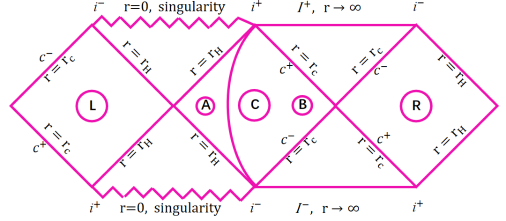
Figure 1: The SdS spacetime with thermal opaque membrane.

Upon review, it was discovered that the SdS spacetime has two physical event horizons associated with different local temperatures, meaning that they cannot reach thermal equilibrium. In order to simplify the analysis, it is crucial to ensure that the system is in thermal equilibrium. The thermal opaque membrane serves this purpose. By employing it, it becomes possible to analyze one horizon with another as the boundary in the multi-event horizon SdS spacetime L36 ; L37 . Therefore, the thermally opaque membrane divides region $C$ into two sub-regions, namely $A$ and $B$ ($C=A\cup B$) in Fig.1. In our model, we consider that the $n$ observers located at the BEH can detect the Hawking radiation at temperature $T_{H}$, while the $m$ observers situated at the CEH can detect the Hawking radiation at temperature $T_{C}$.

The massless Dirac equation can be specifically expressed in the following form L38

$$[\gamma^{a}e_{a}{}^{\mu}(\partial_{\mu}+\Gamma_{\mu})]\Phi=0,$$ (9)

where $\gamma^{a}$ are the Dirac matrices and the four-vectors $e_{a}{}^{\mu}$ is the inverse of the tetrad $e^{a}{}_{\mu}$. Let’s first consider the sub-region $A$ and the causally disconnected region $L$, which faces the BEH in Fig.1. The field quantization in the SdS spacetime can be performed in a similar way to the Unruh effect L38 ; L39 ; L40 ; L41 , and we will not discuss it in detail here. Therefore, one can employ the black hole mode and the Kruskal mode for the quantization of the Dirac field, respectively, and then get the Bogoliubov transformations of the operators in SdS and Kruskal coordinates L38 ; L42 . According to Bogoliubov transformations, the expressions for the Kruskal vacuum state and the excited state in the black hole spacetime are found to be

$$|0_{K_{H}}\rangle = \cos r|0_{A},0_{L}\rangle+\sin r|1_{A},1_{L}\rangle,$$

$$|1_{K_{H}}\rangle = |1_{A},0_{L}\rangle,$$ (10)

with $\cos r=\frac{1}{\sqrt{e^{-\frac{\omega}{T_{H}}}+1}}$. Here, $|n_{A}\rangle$ and $|n_{L}\rangle$ denote the number states corresponding to the fermion outside the event horizon and the antifermion inside the event horizon of the black hole, respectively. Similarly, the expressions of the Kruskal vacuum state and the excited state in the expanding universe can be shown as

$$|0_{K_{C}}\rangle = \cos w|0_{B},0_{R}\rangle+\sin w|1_{B},1_{R}\rangle,$$

$$|1_{K_{C}}\rangle = |1_{B},0_{R}\rangle,$$ (11)

with $\cos w=\frac{1}{\sqrt{e^{-\frac{\omega}{T_{C}}}+1}}$. Due to causal disconnection, the observer in the sub-region $A$ or $B$ cannot detect the modes of regions $L$ and $R$.

III Genuine N-partite entanglement in SdS spacetime

If a state of the N-partite system is not biseparable, it is named a genuinely N-partite entangled state. Here, we introduce the concurrence as a measure for genuine N-partite entanglement. The density matrix for the X-state of the N-partite system in the Hilbert-space orthonormal bases $\{|0,0,...,0\rangle,|0,0,...,1\rangle,...,|1,1,...,1\rangle\}$ can be expressed as

$$\rho_{X}=\left(\!\!\begin{array}[]{cccccccc}\mathcal{M}_{1}&&&&&&&\mathcal{C}_{1}\\ &\mathcal{M}_{2}&&&&&\mathcal{C}_{2}&\\ &&\ddots&&&\mathinner{\mskip 1.0mu\raise 1.0pt\vbox{\kern 7.0pt\hbox{.}}\mskip 2.0mu\raise 4.0pt\hbox{.}\mskip 2.0mu\raise 7.0pt\hbox{.}\mskip 1.0mu}&&\\ &&&\mathcal{M}_{y}&\mathcal{C}_{y}&&&\\ &&&\mathcal{C}_{y}^{*}&\mathcal{N}_{y}&&&\\ &&\mathinner{\mskip 1.0mu\raise 1.0pt\vbox{\kern 7.0pt\hbox{.}}\mskip 2.0mu\raise 4.0pt\hbox{.}\mskip 2.0mu\raise 7.0pt\hbox{.}\mskip 1.0mu}&&&\ddots&&\\ &\mathcal{C}_{2}^{*}&&&&&\mathcal{N}_{2}&\\ \mathcal{C}_{1}^{*}&&&&&&&\mathcal{N}_{1}\end{array}\!\!\right),$$ (20)

with $y=2^{N-1}$. The conditions $\sum_{i}(\mathcal{M}_{i}+\mathcal{N}_{i})=1$ and $|\mathcal{C}_{i}|\leq\sqrt{\mathcal{M}_{i}\mathcal{N}_{i}}$ show that the X-state $\rho_{X}$ is normalized and positive. Genuine N-partite concurrence can be denoted as

$$C(\rho_{X})=2\max\{0,|\mathcal{C}_{i}|-\mu_{i}\},i=1,\ldots,y,$$ (21)

where $\mu_{i}=\sum_{j\neq i}^{y}\sqrt{\mathcal{M}_{j}\mathcal{N}_{j}}$ L43 .

In this paper, we initially consider an N-partite Greenberger-Horne-Zeilinger (GHZ) entangled state with $n$ Kruskal modes $\kappa_{H}$ and $m$ Kruskal modes $\kappa_{C}$,

$$|\psi\rangle_{1,\ldots,N} = \alpha|0_{\kappa_{H}}^{1},0_{\kappa_{H}}^{2},...,0_{\kappa_{H}}^{n},0_{\kappa_{C}}^{1},0_{\kappa_{C}}^{2},...,0_{\kappa_{C}}^{m}\rangle$$

$$+ \sqrt{1-\alpha^{2}}|1_{\kappa_{H}}^{1},1_{\kappa_{H}}^{2},...,1_{\kappa_{H}}^{n},1_{\kappa_{C}}^{1},1_{\kappa_{C}}^{2},...,1_{\kappa_{C}}^{m}\rangle.$$

Here, $n$ ($0<n<N$) and $m$ ($0<m<N$) satisfy the relationship $n+m=N$. To the Kruskal observers, the quantum system consists of $N$ modes. Next, we let the $n$ modes be located at the BEH in the sub-region $A$ of $C$, and the $m$ modes are located at the CEH in the sub-region $B$ of $C$. Due to the Hawking effects of the SdS spacetime, the additional $n$ modes and $m$ modes appear in the region $L$ and the region $R$ in Fig.1, respectively. Using Eqs.(II) and (II), we can rewrite the initial state of Eq.(III) as

$$|\psi\rangle_{1,\ldots,2N} = \alpha\bigg{[}\bigotimes_{i=1}^{n}(\cos r|0^{i}_{A},0^{i}_{L}\rangle+\sin r|1^{i}_{A},1^{i}_{L}\rangle)\bigotimes_{j=1}^{m}(\cos w|0^{j}_{B},0^{j}_{R}\rangle+\sin w|1^{j}_{B},1^{j}_{R}\rangle)\bigg{]}$$

$$+ \sqrt{1-\alpha^{2}}\bigg{[}\bigotimes_{x=1}^{n}(|1^{x}_{A},0^{x}_{L}\rangle)\bigotimes_{y=1}^{m}(|1^{y}_{B},0^{y}_{R}\rangle)\bigg{]}.$$

Since the sub-regions $A$ and $B$ are causally disconnected from the sub-regions $L$ and $R$, we should take the trace over physically inaccessible modes in the sub-regions L and R and then obtain the density operator $\rho_{N}$ as

$$\rho_{N}=\rho_{\bm{A}}+\rho_{\bm{X}}+\rho^{\dagger}_{\bm{X}}+\rho_{\bm{B}},$$ (24)

with

$$\rho_{\bm{A}} = \alpha^{2}\bigg{\{}\bigg{[}\cos^{2n}r\bigotimes_{i=1}^{n}(|0\rangle^{i}_{A}\langle 0|)\bigg{]}\bigg{[}\cos^{2m}w\bigotimes_{j=1}^{m}(|0\rangle^{j}_{B}\langle 0|)\bigg{]}+\bigg{[}\cos^{2n}r\bigotimes_{i=1}^{n}(|0\rangle^{i}_{A}\langle 0|)\bigg{]}$$

$$\times \bigg{[}\cos^{2(m-1)}w\sin^{2}w\bigotimes_{j=1}^{m-1}(|0\rangle^{j}_{B}\langle 0|)|1\rangle^{m}_{B}\langle 1|\bigg{]}+...$$

$$+ \bigg{[}\cos^{2}r\sin^{2(n-1)}r|0\rangle^{1}_{A}\langle 0|\bigotimes_{i=2}^{n}(|1\rangle^{i}_{A}\langle 1|)\bigg{]}\bigg{[}\cos^{2}w\sin^{2(m-1)}w\bigotimes_{j=1}^{m-1}(|1\rangle^{j}_{B}\langle 1|)|0\rangle^{m}_{B}\langle 0|\bigg{]}$$

$$+ \bigg{[}\cos^{2}r\sin^{2(n-1)}r|0\rangle^{1}_{A}\langle 0|\bigotimes_{i=2}^{n}(|1\rangle^{i}_{A}\langle 1|)\bigg{]}\bigg{[}\sin^{2m}w\bigotimes_{j=1}^{m}(|1\rangle^{j}_{B}\langle 1|)\bigg{]}\bigg{]}\bigg{\}},$$

$$\rho_{\bm{X}}=\alpha\sqrt{1-\alpha^{2}}\bigg{[}\cos^{n}r\bigotimes_{i=1}^{n}(|0\rangle^{i}_{A}\langle 1|)\bigg{]}\bigg{[}\cos^{m}w\bigotimes_{j=1}^{m}(|0\rangle^{j}_{B}\langle 1|)\bigg{]},$$

and

$$\rho_{\bm{B}} = \alpha^{2}\bigg{\{}\bigg{[}\cos^{2(n-1)}r\sin^{2}r|1\rangle^{1}_{A}\langle 1|\bigotimes_{i=2}^{n}(|0\rangle^{i}_{A}\langle 0|)\bigg{]}\bigg{[}\cos^{2m}w\bigotimes_{j=1}^{m}(|0\rangle^{j}_{B}\langle 0|)\bigg{]}$$

$$+ \bigg{[}\cos^{2(n-1)}r\sin^{2}r|1\rangle^{1}_{A}\langle 1|\bigotimes_{i=2}^{n}(|0\rangle^{i}_{A}\langle 0|)\bigg{]}\bigg{[}\cos^{2(m-1)}w\sin^{2}w\bigotimes_{j=1}^{m-1}(|0\rangle^{j}_{B}\langle 0|)|1\rangle^{m}_{B}\langle 1|\bigg{]}$$

$$+ ...+\bigg{[}\sin^{2n}r\bigotimes_{i=1}^{n}(|1\rangle^{i}_{A}\langle 1|)\bigg{]}\bigg{[}\cos^{2}w\sin^{2(m-1)}w\bigotimes_{j=1}^{m-1}(|1\rangle^{j}_{B}\langle 1|)|0\rangle^{m}_{B}\langle 0|\bigg{]}\bigg{\}}$$

$$+ \bigg{[}\alpha^{2}\sin^{2n}r\sin^{2m}w+(1-\alpha^{2})\bigg{]}\bigg{[}\bigotimes_{i=1}^{n}(|1\rangle^{i}_{A}\langle 1|)\bigg{]}\bigg{[}\bigotimes_{j=1}^{m}(|1\rangle^{j}_{B}\langle 1|)\bigg{]},$$

which we write in matrix form as

$$\rho_{N}=\left(\!\!\begin{array}[]{cc}\mathcal{M}_{\bm{A}}&\mathcal{M}_{\bm{X}}\\ \mathcal{M}_{\bm{X}}^{T}&\mathcal{M}_{\bm{B}}\\ \end{array}\!\!\right),$$ (27)

in the $2^{N}$ basis

$$\{|0^{1}_{A},...,0^{n}_{A},0^{1}_{B},...0^{m}_{B}\rangle,|0^{1}_{A},...,0^{n}_{A},0^{1}_{B},...0^{m-1}_{B},1^{m}_{B}\rangle,...,|1^{1}_{A},...,1^{n}_{A},1^{1}_{B},...1^{m-1}_{B},0^{m}_{B}\rangle,$$

$$|1^{1}_{A},...,1^{n}_{A},1^{1}_{B},...1^{m}_{B}\rangle\}.$$

The sub-matrixes $\mathcal{M}_{\bm{A}}$, $\mathcal{M}_{\bm{X}}$, and $\mathcal{M}_{\bm{B}}$ are detailed in Appendix A.

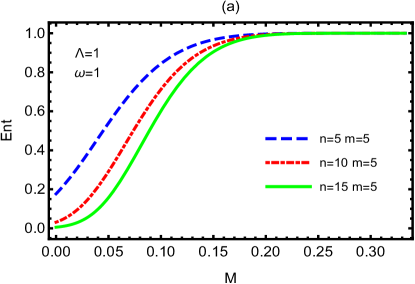
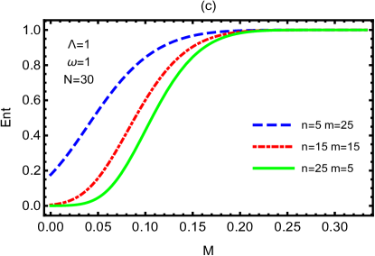
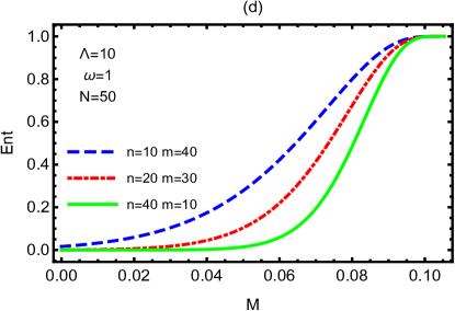
Figure 2: Genuine N-partite entanglement $C(\rho_{N})$ as a function of the mass $M$ of the black hole for different $n$ and $m$, where $\omega=\Lambda=1$.

Employing Eqs.(21) and (27), we obtain the genuine N-partite entanglement measured by the concurrence as

$$C(\rho_{N})=2\cos^{n}r\cos^{m}w\max\bigg{\{}0,\alpha\sqrt{1-\alpha^{2}}-(2^{N-1}-1)\alpha^{2}\sin^{n}r\sin^{m}w\bigg{\}}.$$ (28)

From Eq.(28), it is easy to see that genuine N-partite entanglement depends not only on the initial parameters $\alpha$, $n$, and $m$, but also on the mass $M$ of the black hole and the cosmological constant $\Lambda$.

In Fig.2, we plot genuine N-partite entanglement $C(\rho_{N})$ as a function of the mass $M$ of the black hole for different $n$ and $m$. From Fig.2, we can observe that genuine N-partite entanglement decreases monotonically with the decrease of the mass $M$ of the black hole, meaning that the Hawking effect of the black hole degenerates quantum entanglement. Note that genuine N-partite entanglement recovers to initial value “$2\alpha\sqrt{1-\alpha^{2}}$” at the Nariai limit. This is because the two event horizons do not exist in this limit. We find that genuine N-partite entanglement monotonically decreases with increasing $n$, while it exhibits non-monotonic changes with increasing $m$. Based on the Hawking temperature of the black hole $T_{H}$ being greater than the Hawking temperature of the expanding universe $T_{C}$, it can be concluded that genuine N-partite entanglement increases with the increase of $m$ for a fixed initial total number of particles $N$. In other words, genuine N-partite entanglement monotonically decreases as $n$ increases for a fixed $N$. This conclusion is also supported by Fig.2 (c) and (d).

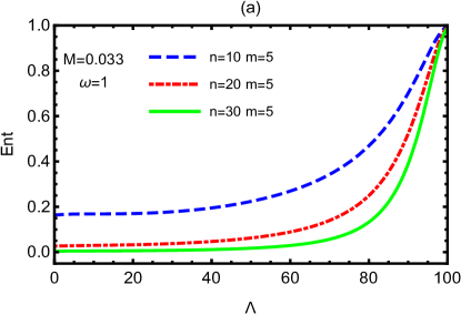
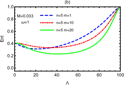
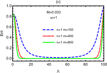
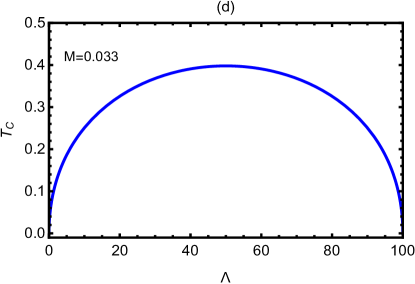
Figure 3: Genuine N-partite entanglement $C(\rho_{N})$ and the Hawking temperature $T_{C}$ of CEH as functions of the cosmological constant $\Lambda$ for different values of $n$ and $m$, where $M=0.033$ and $\omega=1$.

Fig.3 (a)-(c) shows how the cosmological constant $\Lambda$ influences genuine N-partite entanglement $C(\rho_{N})$. From Fig.3 (d), we see that the Hawking temperature $T_{C}$ of CEH changes non-monotonically with $\Lambda$. We find that the Hawking effect of the expanding universe can enhance genuine N-partite entanglement, while the Hawking effect of the black hole only destroys genuine N-partite entanglement in the multi-event horizon spacetime. This results are different from the property of multipartite entanglement in the single-event horizon spacetime L9 ; L10 ; L11 ; L12 ; L13 ; L14 ; L15 ; L16 ; L17 ; L18 ; L19 ; L20 ; L21 . Fig.3 (a)-(c) again shows that genuine N-partite entanglement is a decreasing function with $n$ and a non-monotonic function with $m$.

IV Conclutions

In this paper, we have studied the effect of the Hawking effect of the Schwarzschild-de Sitter (SdS) spacetime on genuine N-partite entanglement of massless Dirac fields shared by $n$ observers near BEH and $m$ ($n+m=N$) observers near CEH. We obtain the general analytical expression of genuine N-partite entanglement for any $n$ and $m$ in the multi-event horizon spacetime. We find that the Hawking effect of the black hole can only degenerate genuine N-partite entanglement, while the Hawking effect of the expanding universe can enhance it. However, the Hawking effect of the single-event horizon spacetime destroys multipartite entanglement L9 ; L10 ; L11 ; L12 ; L13 ; L14 ; L15 ; L16 ; L17 ; L18 ; L19 ; L20 ; L21 . This finding can contribute to a better understanding of the Hawking effect in multi-event horizon spacetime. This is because the Hawking effect of the black holes and the Hawking effect of the expanding universe have different influences on genuine N-partite entanglement. Since the Hawking temperature of the black hole is bigger than the Hawking temperature of the expanding universe, genuine N-partite entanglement increases with the increase of $m$ for a fixed initial parameter $N$. These conclusions demonstrate the observer-dependent nature of genuine N-partite entanglement in the multi-event horizon spacetime and guide multipartite entanglement to deal with relativistic quantum information tasks.

Appendix A Sub-matrixes $\mathcal{M}_{\bm{A}}$, $\mathcal{M}_{\bm{X}}$, and $\mathcal{M}_{\bm{B}}$

By analyzing Eqs.(24) and (27), we find that the matrix $\rho_{N}$ is $2^{N}\times 2^{N}$ dimensions, and the sub-matrixes $\mathcal{M}_{\bm{A}}$, $\mathcal{M}_{\bm{X}}$, and $\mathcal{M}_{\bm{B}}$ are $2^{N-1}\times 2^{N-1}$ dimensions. First, the sub-density operator $\rho_{\bm{A}}$ corresponds to sub-matrix $\mathcal{M}_{\bm{A}}$ in the basis

$$\{|0^{1}_{A},...,0^{n}_{A},0^{1}_{B},...0^{m}_{B}\rangle,|0^{1}_{A},...,0^{n}_{A},0^{1}_{B},...0^{m-1}_{B},1^{m}_{B}\rangle,...,|0^{1}_{A},1^{2}_{A},...,1^{n}_{A},1^{1}_{B},...1^{m-1}_{B},0^{m}_{B}\rangle,$$

$$|0^{1}_{A},1^{2}_{A},...,1^{n}_{A},1^{1}_{B},...1^{m}_{B}\rangle\},$$

where the base corresponding to the element $\alpha^{2}\cos^{2(n-i)}r\sin^{2i}r\cos^{2(m-j)}w\sin^{2j}w$ include $i$ “$1_{A}$” and $j$ “$1_{B}$”,

$$|0^{1}_{A},...,0^{n}_{A},0^{1}_{B},...0^{m}_{B}\rangle\langle 0^{1}_{A},...,0^{n}_{A},0^{1}_{B},...0^{m}_{B}|:\alpha^{2}\cos^{2n}r\cos^{2m}w,$$

$$|0^{1}_{A},...,0^{n}_{A},0^{1}_{B},...0^{m-1}1^{m}_{B}\rangle\langle 0^{1}_{A},...,0^{n}_{A},0^{1}_{B},...0^{m-1}1^{m}_{B}|:\alpha^{2}\cos^{2n}r\cos^{2(m-1)}w\sin^{2}w,...,$$

$$|0^{1}_{A},1^{2}_{A},...,1^{n}_{A},1^{1}_{B},...1^{m-1}_{B},0^{m}_{B}\rangle\langle 0^{1}_{A},1^{2}_{A},...,1^{n}_{A},1^{1}_{B},...1^{m-1}_{B},0^{m}_{B}|:\alpha^{2}\cos^{2}r\sin^{2(n-1)}r\cos^{2}w\times$$

$$\sin^{2(m-1)}w,|0^{1}_{A},1^{2}_{A},...,1^{n}_{A},1^{1}_{B},...1^{m}_{B}\rangle\langle 0^{1}_{A},1^{2}_{A},...,1^{n}_{A},1^{1}_{B},...1^{m}_{B}|:\alpha^{2}\cos^{2}r\sin^{2(n-1)}r\sin^{2m}w.$$

Therefore, the sub-matrix $\mathcal{M}_{\bm{A}}$ can be written as

$$\mathcal{M}_{\bm{A}}=\alpha^{2}\left(\!\!\begin{array}[]{cccc}\cos^{2n}r\cos^{2m}w&&&\\ &\cos^{2n}r\cos^{2(m-1)}w\sin^{2}w&&\\ &&\ddots&\\ &&&\cos^{2}r\sin^{2(n-1)}r\sin^{2m}w\\ \end{array}\!\!\right).$$ (33)

Second, the sub-density operator $\rho_{\bm{X}}$ corresponds to sub-matrix $\mathcal{M}_{\bm{X}}$ that can be easily written as

$$\mathcal{M}_{\bm{X}}=\alpha\sqrt{1-\alpha^{2}}\left(\!\!\begin{array}[]{cccc}&&&\cos^{n}r\cos^{m}w\\ &&0&\\ &\mathinner{\mskip 1.0mu\raise 1.0pt\vbox{\kern 7.0pt\hbox{.}}\mskip 2.0mu\raise 4.0pt\hbox{.}\mskip 2.0mu\raise 7.0pt\hbox{.}\mskip 1.0mu}&&\\ 0&&&\\ \end{array}\!\!\right).$$ (38)

Finally, the sub-density operator $\rho_{\bm{B}}$ can be demonstrated as sub-matrix $\mathcal{M}_{\bm{B}}$ that corresponds to elements

$$|1^{1},0^{2}_{A},...,0^{n}_{A},0^{1}_{B},...,0^{m}_{B}\rangle\langle 1^{1},0^{2}_{A},...,0^{n}_{A},0^{1}_{B},...,0^{m}_{B}|:\rho_{2^{N-1}+1}$$

$$|1^{1},0^{2}_{A},...,0^{n}_{A},0^{1}_{B},...,0^{m-1}_{B},1^{m}_{B}\rangle\langle 1^{1},0^{2}_{A},...,0^{n}_{A},0^{1}_{B},...,0^{m-1}_{B},1^{m}_{B}|:\rho_{2^{N-1}+2},...,$$

$$|1^{1},...,1^{n}_{A},1^{1}_{B},...,1^{m-1}_{B},0^{m}_{B}\rangle\langle 1^{1},...,1^{n}_{A},1^{1}_{B},...,1^{m-1}_{B},0^{m}_{B}|:\rho_{2^{N}-1},$$

$$|1^{1}_{A},...,1^{n}_{A},1^{1}_{B},...1^{m}_{B}\rangle\langle 1^{1}_{A},...,1^{n}_{A},1^{1}_{B},...1^{m}_{B}|:\rho_{2^{N}},$$

where

$$\rho_{2^{N-1}+1}=\alpha^{2}\cos^{2(n-1)}r\sin^{2}r\cos^{2m}w,\rho_{2^{N-1}+2}=\alpha^{2}\cos^{2(n-1)}r\sin^{2}r\cos^{2(m-1)}w\sin^{2}w,$$

$$\rho_{2^{N}-1}=\alpha^{2}\sin^{2n}r\cos^{2}w\sin^{2(m-1)}w,\rho_{2^{N}}=\alpha^{2}\sin^{2n}r\sin^{2m}w+1-\alpha^{2}.$$

Then, the sub-matrix $\mathcal{M}_{\bm{B}}$ can be expressed as

$$\mathcal{M}_{\bm{B}}=\left(\!\!\begin{array}[]{ccccc}\rho_{2^{N-1}+1}&&&&\\ &\rho_{2^{N-1}+2}&&&\\ &&\ddots&\\ &&&\rho_{2^{N}-1}&\\ &&&&\rho_{2^{N}}\\ \end{array}\!\!\right).$$ (44)

References

• (1) M. Hillery, V. BuΕΎek and A. Berthiaume, Phys. Rev. A 59, 1829 (1999).
• (2) N. Gisin, G. Ribordy, W. Tittel and H. Zbinden, Rev. Mod. Phys. 74, 145 (2002).
• (3) A. K. Ekert, Phys. Rev. Lett. 67, 661 (1991).
• (4) C. H. Bennett and S. J. Wiesner, Phys. Rev. Lett. 69, 2881 (1992).
• (5) H. J. Briegel, D. E. Browne, W. DΓΌr, R. Raussendorf, and M. Van den Nest, Nat. Phys. 5, 19 (2009).
• (6) V. Giovannetti, S. Lloyd and L. Maccone, Science 306, 1330 (2004).
• (7) I. J. Membrere, K. Gallock-Yoshimura, L. J. Henderson, R. B. Mann, Adv. Quantum Technol. 6, 2300125 (2023).
• (8) Y. Dai, Z. Shen, and Y. Shi, Phys. Rev. D 94, 025012 (2016).
• (9) S. M. Wu, Y. T. Cai, W. J. Peng, H. S. Zeng, Eur. Phys. J. C 82, 412 (2022).
• (10) Y. Nambu, Y. Osawa, Phys. Rev. D 103, 125007 (2021).
• (11) S. Khan, Journal of Modern Optics 59, 250 (2012).
• (12) J. Wang, and J. Jing, Phys. Rev. A 83, 022314 (2011).
• (13) S. Harikrishnan, S. Jambulingam, P. P. Rohde, C. Radhakrishnan, Phys. Rev. A 105, 052403 (2022).
• (14) T. Zhang, X. Wang, S. M. Fei, Eur. Phys. J. C 83, 607 (2023).
• (15) Z. H. Ma, Z. H. Chen, J. L. Chen, C. Spengler, A. Gabriel, and M. Huber, Phys. Rev. A 83, 062325 (2011).
• (16) S. Xu, X. K. Song, J. D. Shi, and L. Ye, Phys. Rev. D 89, 065022 (2014).
• (17) S. Cepollaro, G. Chirco, G. Cuffaro, V. D’Esposito, Phys. Rev. D 108, 046010 (2023).
• (18) A. J. Torres-Arenas, Q. Dong, G. H. Sun, W. C. Qiang, S. H. Dong, Phys. Lett. B 789, 93 (2019).
• (19) S. M. Wu, H. S. Zeng, Eur. Phys. J. C 82, 4 (2022).
• (20) M. R. Hwang, D. Park, and E. Jung, Phys. Rev. A 83, 012111 (2011).
• (21) W. de Sitter, Proc. Kon. Ned. Akad. Wet. 19, 1217 (1917).
• (22) W. de Sitter, Proc. Kon. Ned. Akad. Wet. 20, 229 (1917).
• (23) S. W. Hawking and G. F. R. Ellis, The Large Scale Structure of Space-Time (Cambridge University Press, Cambridge, England, 1973).
• (24) E. SchrΓΆdinger, Expanding Universes (Cambridge University Press, Cambridge, England, 1956).
• (25) S. M. Wu, C. X. Wang, D. D. Liu, X. L. Huang, H. S. Zeng, J. High Energy Phys. 02, 115 (2023).
• (26) A. G. Riess $et$ $al.$, Astron. J. 116, 1009 (1998).
• (27) S. Perlmutter $et$ $al.$, Astrophys. J. 517, 565 (1999).
• (28) F. Kottler, Ann. Phys. (N.Y.) 361, 401 (1918).
• (29) Z. StuchlΓ­k and S. HledΓ­k, Phys. Rev. D 60, 044006 (1999).
• (30) S. Akcay and R. A. Matzner, Classical Quantum Gravity 28, 085012 (2011).
• (31) W. Rindler, Relativity: Special, General, and Cosmological (Oxford University Press, New York, 2006).
• (32) K. Goswami, K. Narayan, J. High Energy Phys. 10, 031 (2022).
• (33) S. Bhattacharya. A. Lahiri, Eur. Phys. J. C 73, 2673 (2013).
• (34) S. Bhattacharya, N. Joshi, Phys. Rev. D 105, 065007 (2022).
• (35) A. Roy Chowdhury, A. Saha, S. Gangopadhyay, Phys. Rev. D 108, 026003 (2023).
• (36) Q. Liu, S. M. Wu, C. Wen, J. Wang, Sci. China Phys. Mech. Astron. 66, 120413 (2023).
• (37) S. M. Wu, J. X. Li, X. W. Fan, W. M. Li, X. L. Huang, H. S. Zeng, Eur. Phys. J. C 84, 176 (2024).
• (38) A. AragΓ³n, $et$ $al$., Phys. Rev. D 103, 064006 (2021).
• (39) S. Bhattacharya, Phys. Rev. D 98, 125013 (2018).
• (40) P. M. Alsing, I. Fuentes-Schuller, R. B. Mann, and T. E. Tessier, Phys. Rev. A 74, 032326 (2006).
• (41) W. G. Unruh, Phys. Rev. D 14, 870 (1976).
• (42) L. C. B. Crispino, A. Higuchi, and G. E. A. Matsas, Rev. Mod. Phys. 80, 787 (2008).
• (43) I. Fuentes-Schuller and R. B. Mann, Phys. Rev. Lett. 95, 120404 (2005).
• (44) S. M. Wu, X. W. Fan, R. D. Wang, H. Y. Wu, X. L. Huang, H. S. Zeng, J. High Energy Phys. 11, 232 (2023).
• (45) S. M. Hashemi Rafsanjani, M. Huber, C. J. Broadbent, J. H. Eberly, Phys. Rev. A 86, 062303 (2012).