Self-similar imploding solutions of the relativistic Euler equations

Abstract.

Motivated by recent breakthrough on smooth imploding solutions of compressible Euler, we construct self-similar smooth imploding solutions of isentropic relativistic Euler equations with isothermal equation of state $p=\frac{1}{\ell}\varrho$ for all $\ell>1$ in physical space dimension $d=2,3$ and for $\ell>1$ close to 1 in higher dimensions. This work is a crucial step toward solving the long-standing problem: finite time blow-up of the supercritical defocusing nonlinear wave equation.

1. Introduction

In this paper, we consider the relativistic Euler equations, which describe the motion of a relativistic fluid in the flat Minkowski space-time $\mathbb{M}^{1+d}$, $d\geq 1$, with the flat Lorentzian metric $g=(g_{\mu\nu})$ given by

$$g_{00}=-1,\ \ g_{ii}=1\ \ \text{for $1\leq i\leq d$},\ \ g_{\mu\nu}=0\ \ \text{for $\mu\neq\nu$}.$$

The fluid state is represented by the energy density $\varrho\geq 0$, and the relativistic velocity $\vec{u}=(u^{0},u^{1},\cdots,u^{d})$ normalized by

(1.1) $$|\vec{u}|_{g}^{2}=g_{\mu\nu}u^{\mu}u^{\nu}=u_{\mu}u^{\mu}=-1.$$

The motion of the fluid is dominated by the isentropic relativistic Euler equations

(1.2) $$\begin{cases}u^{\mu}\partial_{\mu}\varrho+(p+\varrho)\partial_{\mu}u^{\mu}=0,\\ \partial_{\mu}T^{\mu\nu}=0,\end{cases}$$

where $p$ is the pressure subject to the equation of state $p=p(\varrho)$, and $T^{\mu\nu}$ is the energy-momentum tensor defined by

(1.3) $$T^{\mu\nu}=(p+\varrho)u^{\mu}u^{\nu}+pg^{\mu\nu}.$$

The local-in-time existence of smooth solution for relativistic Euler equations was proved by Makino and Ukai [37]. The first global existence result for the relativistic Euler equations with $d=1$ was obtained by Smoller and Temple [46] under the assumption of bounded total variation of the initial data. The condition regarding bounded total variation is weaken significantly in some recent works [42, 11]. Some results on the singularity formation were obtained by Guo and Tahvildar-Zadeh [28], Pan and Smoller [41] and so on. Christodoulou’s landmark monograph [17] proved the shock formation for open sets of irrotational and isentropic solutions in the 3-D setting, see also [18]. The shock formation for the relativistic Euler equations with non-trivial vorticity and non-constant entropy remains open up to date. A crucial step is made by Disconzi and Speck [21] recently, who rewrite the relativistic Euler equations as a system possessing null structures. For more developments on the mathematical aspects of relativistic fluids, we refer to recent review articles by Abbrescia and Speck [1] and Disconzi [20]. Let’s mention some important works [45, 19, 48, 34, 35] and references therein on the shock formation of compressible Euler equations.

A new blow-up mechanism, known as the implosion, has been constructed in the breakthrough work [39] by Merle, Raphël, Rodnianski and Szeftel for the isentropic compressible Euler equations with $d\geq 2$, where both the density and velocity themselves blow up in finite time. More importantly, in the companion papers [38, 40], they construct radial and asymptotically self-similar blow-up solutions based on smooth self-similar solutions in [39] for both the compressible Navier-Stokes equations and the energy supercritical defocusing nonlinear Schrödinger equations, respectively. In a recent work by Buckmaster, Cao-Labora and Gómez-Serrano [4], the self-similar smooth imploding solutions have been extended to cover a wider range of adiabatic exponents in the 3-D setting. Moreover, non-radial imploding solutions are constructed in [10].

Motivated by breakthrough works [38, 39, 40], we are going to construct self-similar smooth imploding solutions for the isentropic relativistic Euler equations with isothermal equation of state

(1.4) $$p=\frac{1}{\ell}\varrho,$$

where $\ell>1$ corresponds to reciprocal of the square of the sound speed. This equation of state is valid in the early stages of stellar formation, especially $\ell=3$, see Smoller and Temple [46] for more discussions.

Our main result is stated as follows.

Theorem 1.1.

For $k=d-1\geq 1$, there exists a critical $\ell_{*}(k)\in(1,+\infty]$ (see (5.16)) such that for all $1<\ell<\ell_{*}(k)$, we can find a $\beta\in(0,k)$ such that the relativistic Euler equations (1.2) with (1.4) admit a spherically symmetric self-similar solution defined on $[0,T_{*}]\times\mathbb{R}^{d}$, smooth away from the concentrated point $(T_{*},0)$ (where $T_{*}>0$):

(1.5) $$\begin{cases}\varrho(t,x)=\frac{1}{(T_{*}-t)^{\beta}}\hat{\varrho}(Z),\quad u^{0}(t,x)=\widehat{u^{0}}(Z),\quad u^{i}(t,x)=\widehat{u}(Z)\frac{x^{i}}{r}\quad(1\leq i\leq d),\\ r=|x|=\big{(}(x^{1})^{2}+\cdots+(x^{d})^{2}\big{)}^{1/2},\quad Z=r/(T_{*}-t),\end{cases}$$

with the asymptotics

$$\varrho(t,x)=\frac{\varrho_{*}(1+o_{Z\to+\infty}(1))}{|x|^{\beta}},\quad\lim_{Z\to+\infty}\widehat{u^{0}}(Z)=u^{0}_{*},\quad\lim_{Z\to+\infty}\widehat{u}(Z)=u_{*},$$

for some real constants $\varrho_{*}>0,u^{0}_{*}\in\mathbb{R}\setminus\{0\},u_{*}\in\mathbb{R}$.

Several remarks are in order.

1. We have $\ell_{*}(1)=\ell_{*}(2)=+\infty$ and for $3\leq k\leq 6$, the value of $\ell_{*}(k)$ ($=\ell_{1}(k)$, see (5.16)) can be found in Table 1. For $k\geq 3$, the upper bound $\ell_{*}(k)$ is not optimal and can be improved using the method in Section 9. Here we only consider the case $R\in(3,4)$ defined by (4.14), and the upper bound $\ell_{*}(k)$ can be improved by considering larger $R$.

2. Our result is not perturbative, in view of Table 1. Moreover, our proof does not rely on any numerical computations, except for Table 1.

3. Our solution constructed in this paper can be used to construct a finite time blow-up for the supercritical defocusing nonlinear wave equation. Indeed, we consider nonlinear wave equation of the form $\Box u=|u|^{p-1}u$ for the unknown field $u:\mathbb{R}^{1+d}\to\mathbb{C}$, where $\Box=\partial^{\mu}\partial_{\mu}=-\partial_{t}^{2}+\sum_{i=1}^{d}\partial_{i}^{2}$ is the d’Alembertian operator on $\mathbb{R}^{1+d}.$ We write the modular-phase decomposition $u=\rho\mathrm{e}^{\mathrm{i}\phi}$, with $\rho,\phi:\mathbb{R}^{1+d}\to\mathbb{R}$ and $\rho>0$, then

   $$\Box u=(\Box\rho+2\mathrm{i}\partial^{\mu}\rho\partial_{\mu}\phi+\mathrm{i}\rho\Box\phi-\rho\partial^{\mu}\phi\partial_{\mu}\phi)\mathrm{e}^{\mathrm{i}\phi}.$$

   Now we introduce the front renormalization $\rho\mapsto b^{-\frac{1}{p-1}}\rho$, $\phi\mapsto b^{-\frac{1}{2}}\phi$, where $b>0$ is a small number, then the above system becomes

   $$b\Box\rho=\rho^{p}+\rho\partial^{\mu}\phi\partial_{\mu}\phi,\quad 2\partial^{\mu}\rho\partial_{\mu}\phi+\rho\Box\phi=0.$$

   Letting $b\downarrow 0$ gives

   $$\rho^{p}+\rho\partial^{\mu}\phi\partial_{\mu}\phi=0,\quad 2\partial^{\mu}\rho\partial_{\mu}\phi+\rho\Box\phi=0,$$

   or equivalently,

   (1.6) $$\rho^{p-1}+\partial^{\mu}\phi\partial_{\mu}\phi=0,\quad\partial_{\mu}(\rho^{2}\partial^{\mu}\phi)=0.$$

   Let $\ell=1+\frac{4}{p-1}$, $\varrho=\rho^{p+1}$, then (1.6) becomes (2.5) and (2.6), which are deduced from (1.2) in the irrotational regime. After introducing self-similarity and spherical symmetry into (1.6), we can convert (1.6) into an ODE which is exactly the same as (2.17). Therefore, this paper gives a crucial step toward the construction of blow-up solution to the supercritical defocusing nonlinear wave equation, which is the main content of our forthcoming paper [44]. In view of Lemma A.7, it seems that we can prove the blow-up for the nonlinear wave equation for $d=4$ and all $p\geq 29$ and $d=5$ for all $p\geq 17$.

Let’s conclude this introduction by reviewing some recent progress on self-similar type singularities for the fluid PDEs.

Firstly, we refer to [13, 22, 23] and [14, 15, 36] and [12, 16, 29, 30, 31] for the finite time singularity formation of self-similar type on the 3-D incompressible Euler equations and related lower dimensional models. Secondly, in a series of works [7, 5, 6, 8, 9], Buckmaster, Shkoller, Vicol et al developed a systematic approach via constructing asymptotically self-similar solutions to study the formation and development of shocks for the compressible Euler equations even in the presence of vorticity and entropy. Thirdly, there are many recent progress on the gravitational collapse in the field of astrophysics, referring to a process as star implosion, see [25, 27, 24, 2, 26] and references therein. These singularity results are all of self-similar type in the class of radially symmetric solutions, and the key ingredient is to solve some non-autonomous ODEs having sonic points.

2. The self-similar equation and phase portrait

Plugging the equation of state (1.4) into the first equation of (1.2), we obtain

(2.1) $$\partial_{\mu}\left(\varrho^{\frac{\ell}{\ell+1}}u^{\mu}\right)=0.$$

We find the solution of spherical symmetry, which takes

$$\varrho=\varrho(t,r),\quad u^{0}=u^{0}(t,r),\quad u^{i}=u_{r}(t,r)\frac{x^{i}}{r},\quad 1\leq i\leq d,$$

where

$$t=x^{0}\quad\text{and}\quad r=\big{(}(x^{1})^{2}+\cdots+(x^{d})^{2}\big{)}^{1/2}.$$

Under the spherical symmetry, (2.1) is equivalent to

(2.2) $$\partial_{t}\left(\varrho^{\frac{\ell}{\ell+1}}u^{0}\right)+\partial_{r}\left(\varrho^{\frac{\ell}{\ell+1}}u_{r}\right)+\frac{k}{r}\varrho^{\frac{\ell}{\ell+1}}u_{r}=0,$$

where $k=d-1$.

Furthermore, we assume that the fluid is irrotational, i.e.,

(2.3) $$u^{\mu}=\varrho^{-\frac{1}{\ell+1}}\partial^{\mu}\phi$$

for some potential function $\phi$. For spherically symmetric $\phi=\phi(t,r)$, we have $u^{0}=-\varrho^{-\frac{1}{\ell+1}}\partial_{t}\phi$ and $u_{r}=\varrho^{-\frac{1}{\ell+1}}\partial_{r}\phi$, or equivalently,

(2.4) $$\partial_{r}\left(\varrho^{\frac{1}{\ell+1}}u^{0}\right)+\partial_{t}\left(\varrho^{\frac{1}{\ell+1}}u_{r}\right)=0.$$

It follows from (1.1) and (2.3) that

(2.5) $$0=\varrho^{\frac{2}{1+\ell}}+\partial^{\mu}\phi\partial_{\mu}\phi=\varrho^{\frac{2}{1+\ell}}-|\partial_{t}\phi|^{2}+\sum_{i=1}^{d}|\partial_{i}\phi|^{2}.$$

Plugging (2.3) into (2.1), we get

(2.6) $$\partial_{\mu}\left(\varrho^{\frac{\ell-1}{\ell+1}}\partial^{\mu}\phi\right)=0.$$

Now the second equation in (1.2) is automatically satisfied. Indeed, inserting (2.3) and (1.4) into (1.3) gives

$$T^{\mu\nu}=\frac{\ell+1}{\ell}\varrho^{\frac{\ell-1}{\ell+1}}\partial^{\mu}\phi\partial^{\nu}\phi+\frac{1}{\ell}\varrho g^{\mu\nu},$$

and then by (2.5) and (2.6), we get

$$\partial_{\mu}T^{\mu\nu} =\frac{\ell+1}{\ell}\partial_{\mu}\left(\varrho^{\frac{\ell-1}{\ell+1}}\partial^{\mu}\phi\right)\partial^{\nu}\phi+\frac{\ell+1}{\ell}\varrho^{\frac{\ell-1}{\ell+1}}\partial^{\mu}\phi\partial_{\mu}\partial^{\nu}\phi+\frac{1}{\ell}\partial_{\mu}\varrho g^{\mu\nu}$$

$$=\frac{\ell+1}{2\ell}\varrho^{\frac{\ell-1}{\ell+1}}\partial^{\nu}\left(\partial_{\mu}\phi\partial^{\mu}\phi\right)+\frac{1}{\ell}\partial^{\nu}\varrho=-\frac{\ell+1}{2\ell}\varrho^{\frac{\ell-1}{\ell+1}}\partial^{\nu}\left(\varrho^{\frac{2}{\ell+1}}\right)+\frac{1}{\ell}\partial^{\nu}\varrho=0.$$

As a result, it suffices to solve the system consisting of (2.2), (2.4) and

(2.7) $$u^{0}(t,r)^{2}-u_{r}(t,r)^{2}=1$$

for the unknowns $(\varrho,u^{0},u_{r})$.

For each $\beta>0$, the system consisting of (2.2), (2.4) and (2.7) is invariant under the scaling

$$\varrho_{\lambda}(t,r)=\lambda^{\beta}\varrho(\lambda t,\lambda r),\quad u^{0}_{\lambda}(t,r)=u^{0}(\lambda t,\lambda r),\quad u_{r,\lambda}(t,r)=u_{r}(\lambda t,\lambda r),\qquad\lambda>0.$$

We look for solutions $(\varrho(t,r),u^{0}(t,r),u_{r}(t,r))$ that are self-similar:

(2.8) $$\varrho(t,r)=(T_{*}-t)^{-\beta}\widehat{\varrho}(Z),\quad u^{0}(t,r)=\widehat{u^{0}}(Z),\quad u_{r}(t,r)=\widehat{u}(Z),\qquad t\in[0,T_{*}),$$

where $T_{*}>0$ and $Z=r/(T_{*}-t)$. Then we compute (here the prime ^′ represents derivatives with respect to $Z$)

$$\partial_{t}\left(\varrho^{\frac{\ell}{\ell+1}}u^{0}\right)=(T_{*}-t)^{-\frac{\beta\ell}{\ell+1}-1}\left(\frac{\beta\ell}{\ell+1}\widehat{\varrho}^{\frac{\ell}{\ell+1}}\widehat{u^{0}}(Z)+Z\left(\widehat{\varrho}^{\frac{\ell}{\ell+1}}\widehat{u^{0}}\right)^{\prime}(Z)\right),$$

$$\partial_{t}\left(\varrho^{\frac{1}{\ell+1}}u_{r}\right)=(T_{*}-t)^{-\frac{\beta}{\ell+1}-1}\left(\frac{\beta}{\ell+1}\widehat{\varrho}^{\frac{1}{\ell+1}}\widehat{u}(Z)+Z\left(\widehat{\varrho}^{\frac{1}{\ell+1}}\widehat{u}\right)^{\prime}(Z)\right),$$

$$\partial_{r}\left(\varrho^{\frac{\ell}{\ell+1}}u_{r}\right)=(T_{*}-t)^{-\frac{\beta\ell}{\ell+1}-1}\left(\widehat{\varrho}^{\frac{\ell}{\ell+1}}\widehat{u}\right)^{\prime}(Z),$$

$$\partial_{r}\left(\varrho^{\frac{1}{\ell+1}}u^{0}\right)=(T_{*}-t)^{-\frac{\beta}{\ell+1}-1}\left(\widehat{\varrho}^{\frac{1}{\ell+1}}\widehat{u^{0}}\right)^{\prime}(Z),$$

$$\frac{k}{r}\varrho^{\frac{\ell}{\ell+1}}u_{r}=(T_{*}-t)^{-\frac{\beta\ell}{\ell+1}-1}\frac{k}{Z}\widehat{\varrho}^{\frac{\ell}{\ell+1}}\widehat{u}(Z).$$

Hence, (2.2) and (2.4) are equivalent to

$$\frac{\beta\ell}{\ell+1}\widehat{\varrho}^{\frac{\ell}{\ell+1}}\widehat{u^{0}}(Z)+Z\left(\widehat{\varrho}^{\frac{\ell}{\ell+1}}\widehat{u^{0}}\right)^{\prime}(Z)+\left(\widehat{\varrho}^{\frac{\ell}{\ell+1}}\widehat{u}\right)^{\prime}(Z)+\frac{k}{Z}\widehat{\varrho}^{\frac{\ell}{\ell+1}}\widehat{u}(Z)=0,$$

$$\frac{\beta}{\ell+1}\widehat{\varrho}^{\frac{1}{\ell+1}}\widehat{u}(Z)+Z\left(\widehat{\varrho}^{\frac{1}{\ell+1}}\widehat{u}\right)^{\prime}(Z)+\left(\widehat{\varrho}^{\frac{1}{\ell+1}}\widehat{u^{0}}\right)^{\prime}(Z)=0,$$

which are further reduced to

(2.9) $$\frac{\beta\ell}{\ell+1}\widehat{u^{0}}(Z)+Z\widehat{u^{0}}^{\prime}(Z)+\widehat{u}^{\prime}(Z)+\frac{k}{Z}\widehat{u}(Z)+\frac{\ell}{\ell+1}\left(Z\widehat{u^{0}}(Z)+\widehat{u}(Z)\right)\frac{\widehat{\varrho}^{\prime}(Z)}{\widehat{\varrho}(Z)}=0,$$

(2.10) $$\frac{\beta}{\ell+1}\widehat{u}(Z)+Z\widehat{u}^{\prime}(Z)+\widehat{u^{0}}^{\prime}(Z)+\frac{1}{\ell+1}\left(Z\widehat{u}(Z)+\widehat{u^{0}}(Z)\right)\frac{\widehat{\varrho}^{\prime}(Z)}{\widehat{\varrho}(Z)}=0.$$

By (2.7) we have $\widehat{u^{0}}(Z)^{2}-\widehat{u}(Z)^{2}=1$. Let $v(Z)=-\widehat{u}(Z)/\widehat{u^{0}}(Z)$. Then we obtain

(2.11) $$\widehat{u^{0}}(Z)=-\frac{1}{\sqrt{1-v(Z)^{2}}},\quad\widehat{u}(Z)=\frac{v(Z)}{\sqrt{1-v(Z)^{2}}},$$

(2.12) $$\widehat{u^{0}}^{\prime}(Z)=-\frac{v(Z)v^{\prime}(Z)}{(1-v(Z)^{2})^{3/2}},\quad\widehat{u}^{\prime}(Z)=\frac{v^{\prime}(Z)}{(1-v(Z)^{2})^{3/2}}.$$

Here we assume $\widehat{u^{0}}(Z)<0$. Let $m=\frac{\beta\ell}{\ell+1}>0$. Then (2.9) and (2.10) become

(2.13) $$\frac{-m+{kv(Z)}/{Z}}{\sqrt{1-v(Z)^{2}}}+\frac{v^{\prime}(Z)(1-Zv(Z))}{(1-v(Z)^{2})^{3/2}}+\frac{\ell}{\ell+1}\frac{v(Z)-Z}{\sqrt{1-v(Z)^{2}}}\frac{\widehat{\varrho}^{\prime}(Z)}{\widehat{\varrho}(Z)}=0,$$

(2.14) $$\frac{mv(Z)}{\ell\sqrt{1-v(Z)^{2}}}+\frac{v^{\prime}(Z)(Z-v(Z))}{(1-v(Z)^{2})^{3/2}}+\frac{1}{\ell+1}\frac{Zv(Z)-1}{\sqrt{1-v(Z)^{2}}}\frac{\widehat{\varrho}^{\prime}(Z)}{\widehat{\varrho}(Z)}=0.$$

Eliminating $\hat{\varrho}$ from (2.13) and (2.14) gives

(2.15) $$\left[(-m+{kv(Z)}/{Z})\left(1-v(Z)^{2}\right)+{v^{\prime}(Z)(1-Zv(Z))}\right](Zv(Z)-1)$$

$$= \left[mv(Z)(1-v(Z)^{2})+\ell v^{\prime}(Z)(Z-v(Z))\right](v(Z)-Z),$$

which can be rearranged as

(2.16) $$\left[(1-Zv)^{2}-\ell(v-Z)^{2}\right]v^{\prime}(Z)=(1-v^{2})\left[m(1-v^{2})-kv\left(\frac{1}{Z}-v\right)\right],$$

or

(2.17) $$\frac{\mathrm{d}v}{\mathrm{d}Z} =\frac{(1-v^{2})\left[m(1-v^{2})-kv\left(\frac{1}{Z}-v\right)\right]}{(1-Zv)^{2}-\ell(v-Z)^{2}}$$

$$=\frac{(1-v^{2})\left[m(1-v^{2})Z-kv\left(1-vZ\right)\right]}{Z\left[(1-Zv)^{2}-\ell(v-Z)^{2}\right]}=\frac{\Delta_{v}(Z,v)}{\Delta_{Z}(Z,v)},$$

where

$$\Delta_{v}(Z,v)=(1-v^{2})\left[m(1-v^{2})Z-kv\left(1-vZ\right)\right],$$

$$\Delta_{Z}(Z,v)=Z\left[(1-Zv)^{2}-\ell(v-Z)^{2}\right].$$

Lemma 2.1.

If $v(Z):[0,1]\to(-1,1)$ is a $C^{1}$ solution to (2.16) with $v(0)=0$ and $\ell>1$, $m>0$, $k>0$, then $k>m\left(1+\frac{1}{\sqrt{\ell}}\right)$.

Proof.

Let $F(Z)=(1-Zv)+\sqrt{\ell}(v-Z)$. Then $F\in C([0,1])$ is real valued, $F(0)=1>0,$ $F(1)=(\sqrt{\ell}-1)(v(1)-1)<0$. Thus, there exists $Z_{0}\in(0,1)$ such that $F(Z_{0})=0$. Then

$$[(1-Zv)^{2}-\ell(v-Z)^{2}]v^{\prime}|_{Z=Z_{0}}$$

$$= [(1-Zv)+\sqrt{\ell}(v-Z)][(1-Zv)-\sqrt{\ell}(v-Z)]v^{\prime}|_{Z=Z_{0}}$$

$$= F(Z_{0})[(1-Zv)-\sqrt{\ell}(v-Z)]v^{\prime}|_{Z=Z_{0}}=0,$$

which gives $(1-v^{2})[m(1-v^{2})-kv(1/Z-v)]|_{Z=Z_{0}}=0$. Let $v_{0}=v(Z_{0})$. Then $v_{0}\in(-1,1)$, and $(1-v_{0}^{2})[m(1-v_{0}^{2})-kv_{0}(1/Z_{0}-v_{0})]=0,$ thus $m(1-v_{0}^{2})-kv_{0}(1/Z_{0}-v_{0})=0$. This implies that $v_{0}\in(0,1)$, since otherwise $v_{0}\in(-1,0]$, hence $m(1-v_{0}^{2})>0$ but $kv_{0}(1/Z_{0}-v_{0})\leq 0$, a contradiction. We also have $0=F(Z_{0})=(1-Z_{0}v_{0})+\sqrt{\ell}(v_{0}-Z_{0})$, so $Z_{0}=\frac{1+\sqrt{\ell}v_{0}}{\sqrt{\ell}+v_{0}}$. Hence,

$$k =\frac{m(1-v_{0}^{2})}{v_{0}\left(\frac{1}{Z_{0}}-v_{0}\right)}=\frac{m(1-v_{0}^{2})}{v_{0}\left(\frac{\sqrt{\ell}+v_{0}}{1+\sqrt{\ell}v_{0}}-v_{0}\right)}=\frac{m(1-v_{0}^{2})}{v_{0}\frac{\sqrt{\ell}(1-v_{0}^{2})}{1+\sqrt{\ell}v_{0}}}$$

$$=\frac{m(1+\sqrt{\ell}v_{0})}{\sqrt{\ell}v_{0}}=\frac{m}{\sqrt{\ell}}\left(\frac{1}{v_{0}}+\sqrt{\ell}\right)>\frac{m}{\sqrt{\ell}}(1+\sqrt{\ell})=m\left(1+\frac{1}{\sqrt{\ell}}\right).$$

This completes the proof. ∎

In view of the above lemma, it is natural to restrict the parameters $(m,\ell,k)$ in the following regime

(2.18) $$m>0,\qquad\ell>1,\qquad k\in\mathbb{Z}_{+},\qquad k>m\left(1+\frac{1}{\sqrt{\ell}}\right).$$

The solutions to $\Delta_{v}(Z,v)=0$ are $v=\pm 1$ and

(2.19) $$v_{1}(Z)=\frac{k-\sqrt{k^{2}-4(k-m)mZ^{2}}}{2(k-m)Z},\qquad v_{2}(Z)=\frac{k+\sqrt{k^{2}-4(k-m)mZ^{2}}}{2(k-m)Z}$$

for $|Z|\leq Z_{e}=\frac{k}{2\sqrt{(k-m)m}}$, which is equivalent to $Z=Z_{\text{b}}(v)=\frac{kv}{m+(k-m)v^{2}}$, see the black curve passing $P_{1}$ in Figure 1. The solutions to $\Delta_{Z}(Z,v)=0$ are $Z=0$ and

(2.20) $$v_{+}(Z)=\frac{\sqrt{\ell}Z+1}{Z+\sqrt{\ell}},\qquad v_{-}(Z)=\frac{-\sqrt{\ell}Z+1}{Z-\sqrt{\ell}}.$$

As a result, it is easy to find that the solutions to $\Delta_{v}=\Delta_{Z}=0$ are

$$P_{0} =(Z=0,v=0),\qquad P_{1}=\left(Z_{1}=\frac{k\sqrt{\ell}}{\ell(k-m)+m},v_{1}=\frac{m}{(k-m)\sqrt{\ell}}\right),$$

$$P_{2} =(Z=1,v=1),\qquad P_{3}=(Z=0,v=1),$$

and $P_{-j}=-P_{j}$ for $j=1,2,3$.

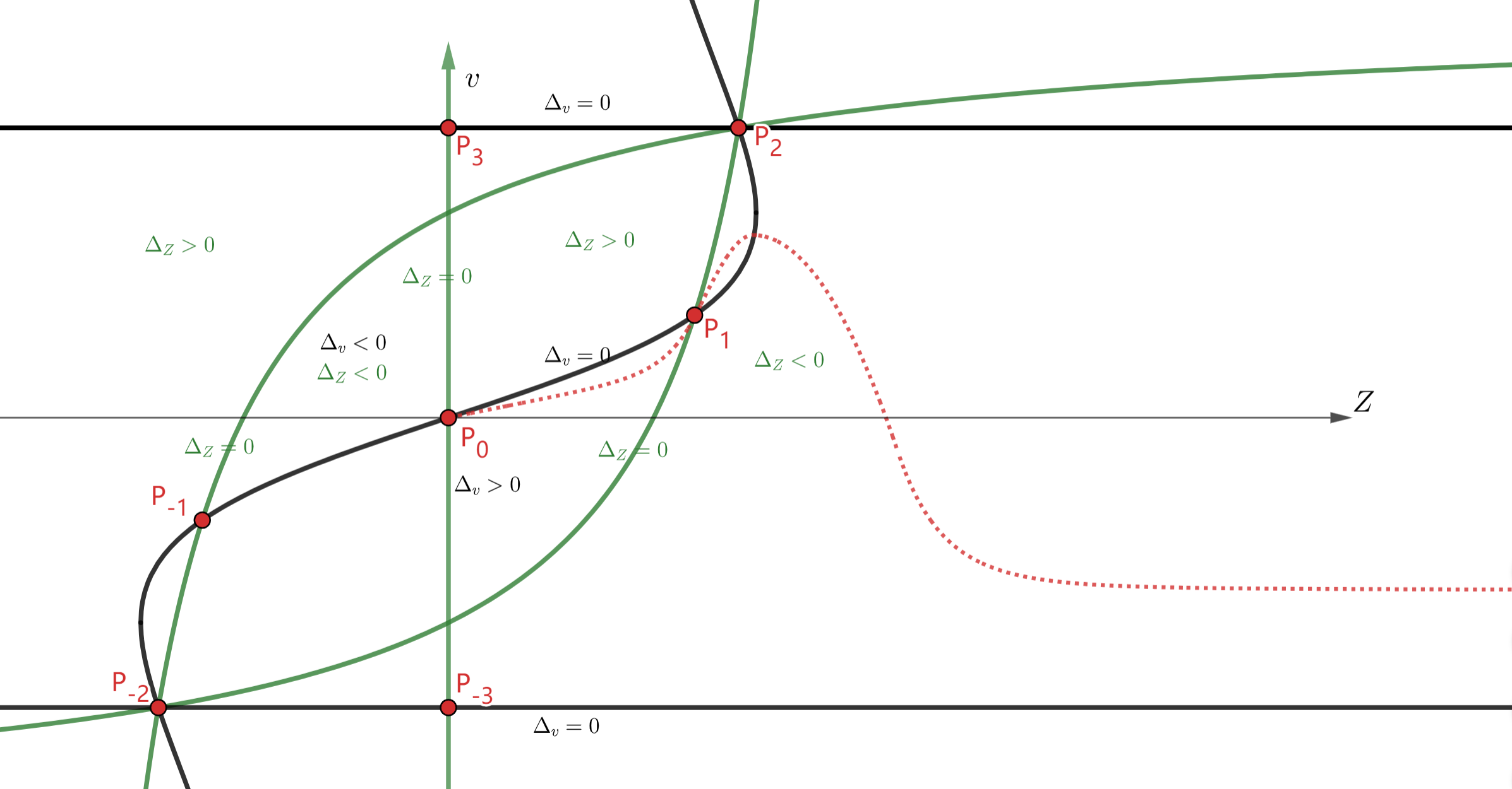
Figure 1. Phase portrait for the $Z-v$ system, with $m=1,\ell=2$ and $k=3$.

Note that the condition (2.18) implies that $0<Z_{1}<1$ and $0<v_{1}<1$. For $Z\in(0,Z_{e})$, we have $0<v_{1}(Z)<v_{2}(Z)$; moreover, it follows from $m(1-v_{1}^{2})Z-kv_{1}(1-v_{1}Z)=(k-m)Zv_{1}^{2}-kv_{1}+mZ=0$ that

$$v_{1}^{\prime}(Z)=-\frac{m+(k-m)v_{1}^{2}(Z)}{2(k-m)Zv_{1}(Z)-k}=\frac{\frac{k}{Z}v_{1}(Z)}{\sqrt{k^{2}-4(k-m)mZ^{2}}}>0$$

and similarly $v_{2}^{\prime}(Z)=-\frac{\frac{k}{Z}v_{2}(Z)}{\sqrt{k^{2}-4(k-m)mZ^{2}}}<0$ for $Z\in(0,Z_{e})$. On the other hand, we have

$$\sqrt{k^{2}-4(k-m)mZ_{1}^{2}} =\sqrt{\frac{k^{2}(\ell(k-m)+m)^{2}-4(k-m)mk^{2}\ell}{(\ell(k-m)+m)^{2}}}$$

$$=\sqrt{\frac{k^{2}(\ell(k-m)-m)^{2}}{(\ell(k-m)+m)^{2}}}=\frac{k(\ell(k-m)-m)}{\ell(k-m)+m},$$

where we have used (2.18) to get $\frac{k}{m}>1+\frac{1}{\sqrt{\ell}}>1+\frac{1}{\ell}$ and hence $\ell(k-m)-m>0$, thus

$$v_{1}(Z_{1})=\frac{k-\frac{k(\ell(k-m)-m)}{\ell(k-m)+m}}{2(k-m)\frac{k\sqrt{\ell}}{\ell(k-m)+m}}=\frac{2km}{2(k-m)k\sqrt{\ell}}=v_{1}.$$

Therefore, the point $P_{1}$ lies on the graph of $v_{1}$, and we have

(2.21) $$v_{1}^{\prime}(Z)>0,\qquad\text{for}\qquad Z\in(0,Z_{1})\subset(0,Z_{e}).$$

Finally, it is easy to check that the point $P_{1}$ lies on the graph of $v_{-}$ and

(2.22) $$v_{+}^{\prime}(Z)=\frac{\ell-1}{(Z+\sqrt{\ell})^{2}}>0,\qquad v_{-}^{\prime}(Z)=\frac{\ell-1}{(Z-\sqrt{\ell})^{2}}>0$$

in view of (2.18). For further usage, we write $v_{-}(Z)$ as $Z_{g}(v)=\frac{\sqrt{\ell}v+1}{v+\sqrt{\ell}}$, see the green curve passing $P_{1}$ in Figure 1.

Our aim in this paper is to show the existence of a $C^{\infty}$ solution to the $Z-v$ ODE (2.17).

Theorem 2.2.

Let $k=d-1\geq 1$. Then there exists $\ell_{*}(k)\in(1,+\infty]$ such that for any $1<\ell<\ell_{*}(k)$, there exists $\beta\in(0,k)$ such that (2.17) with this $\beta$ admits a global $C^{\infty}([0,+\infty))$ solution $v=v(Z)$ defined on $Z\in[0,+\infty)$ satisfying $v(0)=0$ and $|v(Z)|<1$ for all $Z\in[0,+\infty)$; moreover, we have $\Delta_{Z}(Z,v(Z))>0$ for $Z\in(0,Z_{1})$, $\Delta_{Z}(Z,v(Z))<0$ for $Z\in(Z_{1},+\infty)$, $v(Z_{1})=Z_{1}$ and $v(Z)<Z$ for all $Z\in(0,+\infty)$. See the dashed red curve in Figure 1.

Theorem 1.1 is a corollary of Theorem 2.2, see Section 8. Now let’s give a sketch of the proof of Theorem 2.2.

The first step is to construct a smooth local solution to (2.17) starting at $(0,0)$ and show that this solution can be extended until reaching $P_{1}$, and we denote it by $v_{F}$. However, we don’t know anything about the smoothness at $P_{1}$ of $v_{F}$. Our strategy, alike [39], is to construct a smooth local solution $v_{L}$ near $P_{1}$, and to show $v_{L}=v_{F}$, hence $v_{F}$ is smooth at $P_{1}$. Due to high nonlinearity in the $Z-v$ ODE, we will introduce a renormalization $(Z,v)\mapsto(z,u)$, which converts the $Z-v$ ODE to a $z-u$ ODE, see (3.11), and we will find the corresponding curve of $v_{F}$ in the $z-u$ plane, denoted by $u_{F}$, which is a smooth curve connecting $Q_{0}$ to $Q_{1}$, see Figure 2. See Section 3 for the details.

The second step is to construct the local smooth solution $u_{L}$ to the $z-u$ ODE near $Q_{1}$, using the power series method. Then through the inverse mapping of the renormalization, we get a local solution $v_{L}$ to the $Z-v$ ODE near $P_{1}$. This is our main goal in Section 4.

The third step is to show that $u_{L}=u_{F}$, hence $v_{L}=v_{F}$. However, this is not true for some parameters. By analyzing the coefficients of the power series defining $u_{L}$ and using the barrier function method, we can show that for fixed $k\geq 1$ and $\ell\in(1,\ell_{*}(k))$ (not for all $\ell>1$), there exists $\zeta_{0}$ such that for some $\beta_{1}$ we have $u_{L}(\zeta_{0})>u_{F}(\zeta_{0})$, and for some $\beta_{2}$ we have $u_{L}(\zeta_{0})<u_{F}(\zeta_{0})$, hence by the continuous dependence on parameters, the intermediate value theorem gives a $\beta_{0}$ such that for this $\beta_{0}$ we have $u_{L}(\zeta_{0})=u_{F}(\zeta_{0})$. Then by the uniqueness of solutions to ODEs at regular points, we have $u_{L}\equiv u_{F}$. This task will be done in Sections 5 and 6. We will enclose the treatment of $\ell_{*}(k)$ in appendix A. We emphasize that for $k=2$ and $\ell$ large, we need to modify the barrier functions used in Sections 5 and 6, see Section 9 for the details.

Finally, we show that the $P_{0}-P_{1}$ curve $v_{F}$, after passing $P_{1}$ smoothly, will then pass through the black curve $Z=Z_{\text{b}}(v)$ and then be defined on the whole half-line $Z\in[0,+\infty)$. Here we use the barrier function method to exclude the possibility of touching the green curve $Z_{g}(v)$ or $P_{2}$. See Section 7 for the details.

In Section 8, we will combine all things to give a proof of Theorem 2.2.

3. Construction of $P_{0}-P_{1}$ curve and renormalization

In this section, we construct the unique solution $v=v_{F}(Z)$ to (2.17) connecting $P_{0}$ and $P_{1}$. After a renormalization introduced in Subsection 3.2, the $Z-v$ ODE (2.17) is transformed into a $z-u$ ODE, see (3.11), which is easier to analyze when we consider the analytic solutions crossing the sonic point. Before we analyze the analytic solutions of the $z-u$ ODE crossing the sonic point $Q_{1}$, we will show in Subsection 3.3 that the $P_{0}-P_{1}$ solution to the $Z-v$ ODE (2.17) is transformed by the renormalization mapping (3.10) into a $Q_{0}-Q_{1}$ solution to the $z-u$ ODE.

3.1. The $P_{0}-P_{1}$ curve

Here we construct the unique solution $v=v_{F}(Z)$ to (2.17) connecting $P_{0}$ and $P_{1}$. The main idea is to first construct a local solution near the origin $P_{0}$ using the power series method, then prove that this local solution can be continued up to $P_{1}$. We recall the classical theory on the extension of the solutions to ODEs.

Proposition 3.1.

Consider the initial value problem

(3.1) $$\frac{\mathrm{d}\bm{x}}{\mathrm{d}t}=\bm{f}(t,\bm{x}),\qquad\bm{x}(t_{0})=\bm{x_{0}},$$

where $\bm{f}\in{C^{1}}(U;\mathbb{R}^{n})$, $U\subset\mathbb{R}^{1+n}$ is an open set and $(t_{0},\bm{x_{0}})\in U$. Let $I=(T_{-},T_{+})$ be the maximal interval of existence of a solution to (3.1). If $T_{+}<+\infty$, then the solution must eventually leave every compact set $C$ with $[t_{0},T_{+}]\times C\subset U$ as $t$ approaches $T_{+}$.

The proof of Proposition 3.1 can be found in section 2.6 of the classical textbook [47].

Remark 3.2.

If $T_{+}<+\infty$ and the limit $\bm{x}_{*}:=\lim_{T\uparrow T_{+}}\bm{x}(t)$ exists, then $(T_{+},\bm{x}_{*})\not\in U$.

Proposition 3.3.

The ODE

(3.2) $$\frac{\mathrm{d}v}{\mathrm{d}Z}=\frac{(1-v^{2})\left[m(1-v^{2})Z-kv\left(1-vZ\right)\right]}{Z\left[(1-Zv)^{2}-\ell(v-Z)^{2}\right]}=\frac{\Delta_{v}(Z,v)}{\Delta_{Z}(Z,v)}$$

has a unique solution $v\in C^{\infty}([0,Z_{1}))$ with $v(0)=0$.

Proof.

Step 1. Existence of local solution.

Let $\Phi=\frac{v}{Z}$, which satisfies

$$\Phi+Z\frac{\mathrm{d}\Phi}{\mathrm{d}Z} =\frac{\mathrm{d}v}{\mathrm{d}Z}=\frac{(1-Z^{2}\Phi^{2})\left[m(1-Z^{2}\Phi^{2})-k(\Phi-Z^{2}\Phi^{2})\right]}{(1-Z^{2}\Phi)^{2}-\ell(1-\Phi)^{2}Z^{2}}$$

$$=\frac{m-k\Phi+(k-2m)Z^{2}\Phi^{2}+kZ^{2}\Phi^{3}+(m-k)Z^{4}\Phi^{4}}{1-\ell Z^{2}+2(\ell-1)Z^{2}\Phi-\ell Z^{2}\Phi^{2}+Z^{4}\Phi^{2}},$$

which gives

$$\left[1-\ell Z^{2}+2(\ell-1)Z^{2}\Phi-\ell Z^{2}\Phi^{2}+Z^{4}\Phi^{2}\right]Z\frac{\mathrm{d}\Phi}{\mathrm{d}Z}=m-(k+1)\Phi$$

$$\qquad+\ell Z^{2}\Phi+(k-2m-2\ell+2)Z^{2}\Phi^{2}+(k+\ell)Z^{2}\Phi^{3}-Z^{4}\Phi^{3}+(m-k)Z^{4}\Phi^{4}.$$

Let $\varkappa=Z^{2}$. Then $Z\frac{\mathrm{d}\Phi}{\mathrm{d}Z}=2\varkappa\frac{\mathrm{d}\Phi}{\mathrm{d}\varkappa}$, and the above ODE is equivalent to

$$2\left[1-\ell\varkappa+2(\ell-1)\varkappa\Phi-\ell\varkappa\Phi^{2}+\varkappa^{2}\Phi^{2}\right]\varkappa\frac{\mathrm{d}\Phi}{\mathrm{d}\varkappa}=m-(k+1)\Phi$$

$$\qquad+\ell\varkappa\Phi+(k-2m-2\ell+2)\varkappa\Phi^{2}+(k+\ell)\varkappa\Phi^{3}-\varkappa^{2}\Phi^{3}+(m-k)\varkappa^{2}\Phi^{4},$$

which can be further rewritten as

(3.3) $$2\varkappa\frac{\mathrm{d}\Phi}{\mathrm{d}\varkappa}+(k+1)\Phi=G,$$

where

$$G =m+\ell\varkappa\Phi+(k-2m-2\ell+2)\varkappa\Phi^{2}+(k+\ell)\varkappa\Phi^{3}-\varkappa^{2}\Phi^{3}+(m-k)\varkappa^{2}\Phi^{4}$$

$$\qquad-2\left[-\ell\varkappa+2(\ell-1)\varkappa\Phi-\ell\varkappa\Phi^{2}+\varkappa^{2}\Phi^{2}\right]\varkappa\frac{\mathrm{d}\Phi}{\mathrm{d}\varkappa}.$$

We plug the formal expansion

$$\Phi=\sum_{n=0}^{\infty}\phi_{n}\varkappa^{n},\qquad G=\sum_{n=0}^{\infty}g_{n}\varkappa^{n}$$

into (3.3), then we get $(k+1+2n)\phi_{n}=g_{n}$ for each $n\geq 0$. For a function $f$, we denote $f_{n}=\frac{f^{(n)}(0)}{n!}$, then by Leibniz’s rule,

(3.4) $$(fg)_{n}=\frac{1}{n!}\frac{\mathrm{d}^{n}}{\mathrm{d}\varkappa^{n}}(fg)(0)=\frac{1}{n!}\sum_{n_{1}+n_{2}=n}\frac{n!}{n_{1}!n_{2}!}f^{(n_{1})}(0)g^{(n_{2})}(0)=\sum_{n_{1}+n_{2}=n}f_{n_{1}}g_{n_{2}}.$$

Therefore, (3.3) yields the induction relation: $(k+1)\phi_{0}=m$ and for $n\geq 1$,

$$(k+1+2n)\phi_{n}= \ell\phi_{n-1}+(k-2m-2\ell+2)\sum_{n_{1}+n_{2}=n-1}\phi_{n_{1}}\phi_{n_{2}}$$

$$+(k+\ell)\sum_{n_{1}+n_{2}+n_{3}=n-1}\phi_{n_{1}}\phi_{n_{2}}\phi_{n_{3}}-\sum_{n_{1}+n_{2}+n_{3}=n-2}\phi_{n_{1}}\phi_{n_{2}}\phi_{n_{3}}$$

(3.5) $$+(m-k)\sum_{n_{1}+n_{2}+n_{3}+n_{4}=n-2}\phi_{n_{1}}\phi_{n_{2}}\phi_{n_{3}}\phi_{n_{4}}+2\ell(n-1)\phi_{n-1}$$

$$-4(\ell-1)\sum_{n_{1}+n_{2}=n-1}\phi_{n_{1}}(n_{2}\phi_{n_{2}})+2\ell\sum_{n_{1}+n_{2}+n_{3}=n-1}\phi_{n_{1}}\phi_{n_{2}}(n_{3}\phi_{n_{3}})$$

$$-2\sum_{n_{1}+n_{2}+n_{3}=n-2}\phi_{n_{1}}\phi_{n_{2}}(n_{3}\phi_{n_{3}}).$$

Next we prove that the corresponding power series is analytic in a small neighborhood of the origin. We inductively assume that for some $n\geq 1$ we have

$$|\phi_{i}|\leq\mathfrak{C}_{i}M^{i}\quad\text{for all \ }0\leq i\leq n-1,$$

where $M>1$ is a big constant to be determined later, and $\mathfrak{C}_{i}$ denotes the Catalan numbers defined by $\mathfrak{C}_{0}=1$ and the recurrence relation $\mathfrak{C}_{n}=\sum_{i=1}^{n}\mathfrak{C}_{i-1}\mathfrak{C}_{n-i}$ for $n\geq 1$. Combining the Catalan $k$-fold convolution formula (see Lemma 27 in [3])

$$\sum_{i_{1}+\cdots+i_{m}=n\atop i_{1},\ldots,i_{m}\geq 0}\mathfrak{C}_{i_{1}}\cdots\mathfrak{C}_{i_{m}}=\begin{cases}\displaystyle\frac{m(n+1)(n+2)\cdots(n+m/2-1)}{2(n+m/2+2)(n+m/2+3)\cdots(n+m)}\mathfrak{C}_{n+\frac{m}{2}},&m\text{ even,}\\ \displaystyle\frac{m(n+1)(n+2)\cdots(n+(m-1)/2)}{(n+(m+3)/2)(n+(m+3)/2+1)\cdots(n+m)}\mathfrak{C}_{n+\frac{m-1}{2}},&m\text{ odd}\end{cases}$$

with $\mathfrak{C}_{n-1}\sim\mathfrak{C}_{n}$, (3.5) and the inductive assumption, we infer

$$\frac{|\phi_{n}|}{\mathfrak{C}_{n}M^{n}} \leq\frac{C_{0}}{nM}+\frac{C_{0}}{nM\mathfrak{C}_{n}}\sum_{n_{1}+n_{2}=n-1}\mathfrak{C}_{n_{1}}\mathfrak{C}_{n_{2}}+\frac{C_{0}}{nM\mathfrak{C}_{n}}\sum_{n_{1}+n_{2}+n_{3}=n-1}\mathfrak{C}_{n_{1}}\mathfrak{C}_{n_{2}}\mathfrak{C}_{n_{3}}$$

$$\qquad+\frac{C_{0}}{nM^{2}\mathfrak{C}_{n}}\sum_{n_{1}+n_{2}+n_{3}=n-2}\mathfrak{C}_{n_{1}}\mathfrak{C}_{n_{2}}\mathfrak{C}_{n_{3}}+\frac{C_{0}}{nM^{2}\mathfrak{C}_{n}}\sum_{n_{1}+n_{2}+n_{3}+n_{4}=n-2}\mathfrak{C}_{n_{1}}\mathfrak{C}_{n_{2}}\mathfrak{C}_{n_{3}}\mathfrak{C}_{n_{4}}$$

$$\qquad+\frac{C_{0}}{M}+\frac{C_{0}}{M\mathfrak{C}_{n}}\sum_{n_{1}+n_{2}=n-1}\mathfrak{C}_{n_{1}}\mathfrak{C}_{n_{2}}+\frac{C_{0}}{M\mathfrak{C}_{n}}\sum_{n_{1}+n_{2}+n_{3}=n-1}\mathfrak{C}_{n_{1}}\mathfrak{C}_{n_{2}}\mathfrak{C}_{n_{3}}$$

$$\qquad+\frac{C_{0}}{M^{2}\mathfrak{C}_{n}}\sum_{n_{1}+n_{2}+n_{3}=n-2}\mathfrak{C}_{n_{1}}\mathfrak{C}_{n_{2}}\mathfrak{C}_{n_{3}}$$

$$\leq\frac{2C_{0}}{M}+\frac{2C_{0}}{M\mathfrak{C}_{n}}\mathfrak{C}_{n}+\frac{2C_{0}}{M\mathfrak{C}_{n}}\frac{3n}{n+2}\mathfrak{C}_{n}+\frac{2C_{0}}{M^{2}\mathfrak{C}_{n}}\frac{3(n-1)}{n+1}\mathfrak{C}_{n-1}+\frac{C_{0}}{nM^{2}\mathfrak{C}_{n}}\frac{2(n-1)}{n+2}\mathfrak{C}_{n}$$

$$\leq\frac{C_{1}}{M},$$

where $C_{0},C_{1}>0$ are constants independent of $n$ and $M$. Hence, by taking $M>C_{1}$, we obtain $|\phi_{n}|\leq\mathfrak{C}_{n}M^{n}$, and then close the induction. Due to $\mathfrak{C}_{n}\leq 4^{n}$, we know that the power series $\Phi(\varkappa)=\sum_{n=0}^{\infty}\phi_{n}\varkappa^{n}$ is analytic in a small neighborhood of the origin $\varkappa=0$, i.e., $Z=0$. Recalling that $v(Z)=Z\Phi(Z^{2})$, we have proved that the ODE

$$\frac{\mathrm{d}v}{\mathrm{d}Z}=\frac{(1-v^{2})\left[m(1-v^{2})Z-kv\left(1-vZ\right)\right]}{Z\left[(1-Zv)^{2}-\ell(v-Z)^{2}\right]}=\frac{\Delta_{v}(Z,v)}{\Delta_{Z}(Z,v)}$$

has an unique analytic local solution $v=v(Z),Z\in[0,\varepsilon_{0}]$ for some small $\varepsilon_{0}>0$ with the asymptotics

$$v(Z)=\frac{m}{k+1}Z+\phi_{1}Z^{3}+O(Z^{5})\quad\text{as }\quad Z\downarrow 0,$$

where $\phi_{1}$ is given by

(3.6) $$(k+3)\phi_{1}=\ell\phi_{0}+(k-2m-2\ell+2)\phi_{0}^{2}+(k+\ell)\phi_{0}^{3}.$$

Step 2. Extension up to $P_{1}$.

Let $v_{F}=v_{F}(Z)$ be the unique curve entering $P_{0}$ constructed as above. It follows from the asymptotic behavior of $v_{F}$ that

$$\Delta_{v}(Z,v_{F}(Z))=(1-v_{F}^{2})\left((k-m)Zv_{F}^{2}-kv_{F}+mZ\right)=\frac{m}{k+1}Z+O(Z^{3})\quad\text{as }\quad Z\downarrow 0,$$

and $v_{F}^{\prime}(Z)>0$ if $Z\in(0,\widetilde{\varepsilon}_{0})$ for some small $\widetilde{\varepsilon}_{0}\in(0,\varepsilon_{0})$, hence $\Delta_{Z}(Z,v_{F}(Z))>0$ for $Z\in(0,\widetilde{\varepsilon}_{0})$. It follows from (2.19) and (2.20) that $v_{-}(0)=-\frac{1}{\sqrt{\ell}}<0$ and $v_{1}(Z)\sim\frac{m}{k}Z$ as $Z\downarrow 0$, so

$$v_{-}(Z)<v_{F}(Z)<v_{1}(Z)\qquad\text{for }\quad Z\in(0,\widetilde{\varepsilon}_{0})$$

by adjusting $\widetilde{\varepsilon}_{0}>0$ to a smaller number if necessary. We consider the open region

$$\mathcal{R}_{F}=\left\{(Z,v):v_{-}(Z)<v<v_{1}(Z),\ Z\in(0,Z_{1})\right\}.$$

In the region $\mathcal{R}_{F}$, we have $\Delta_{v}>0$ and $\Delta_{Z}>0$. Assume that the maximal interval of existence of the solution $v_{F}$ (such that $(Z,v)\in\mathcal{R}_{F}$) is $(0,Z_{0})$. Then $Z_{0}\in(0,Z_{1}]$, $(Z,v_{F}(Z))\in\mathcal{R}_{F}$, $v_{F}^{\prime}(Z)=\frac{\Delta_{v}(Z,v_{F}(Z))}{\Delta_{Z}(Z,v_{F}(Z))}>0$ for $Z\in(0,Z_{0})$. Thus, the limit $v_{0}:=\lim_{Z\uparrow Z_{0}}v_{F}(Z)$ exists, and $v_{-}(Z_{0})\leq v_{0}\leq v_{1}(Z_{0})$. By Remark 3.2, we have $(Z_{0},v_{0})\not\in\mathcal{R}_{F}$. If $Z_{0}\in(0,Z_{1})$, then

• either $v_{0}=v_{-}(Z_{0})$, in which case we have $v_{F}^{\prime}(Z_{0})=\lim_{Z\uparrow Z_{0}}v_{F}^{\prime}(Z)=+\infty$, and we have a contradiction since $v_{-}(Z)<v_{F}(Z)$ for all $Z\in(0,Z_{0})$, which implies

  $$\frac{v_{F}(Z)-v_{F}(Z_{0})}{Z-Z_{0}}=\frac{v_{F}(Z)-v_{-}(Z_{0})}{Z-Z_{0}}<\frac{v_{-}(Z)-v_{-}(Z_{0})}{Z-Z_{0}},\ \ \text{for all }\ Z\in(0,Z_{0});$$

• or $v_{0}=v_{1}(Z_{0})$, in which case we have $v_{F}^{\prime}(Z_{0})=\lim_{Z\uparrow Z_{0}}v_{F}^{\prime}(Z)=0$, and we also have a contradiction since $v_{F}(Z)<v_{1}(Z)$ for all $Z\in(0,Z_{0})$ and $v_{1}^{\prime}(Z_{0})>0$.

Therefore, $Z_{0}=Z_{1}$, the curve $v_{F}(Z)$ is defined on $[0,Z_{1})$ and $C^{\infty}$ on this interval, and also satisfies $(Z,v_{F}(Z))\in\mathcal{R}_{F}$, $v_{F}^{\prime}(Z)>0$ and (using $0<v_{1}(Z)<v_{1}(Z_{1})=v_{1}=v_{-}(Z_{0})<1$)

(3.7) $$\Delta_{v}(Z,v_{F}(Z))>0,\quad\Delta_{Z}(Z,v_{F}(Z))>0,\quad v_{F}(Z)\in(0,1),\quad\text{for }\ Z\in(0,Z_{1}),$$

(3.8) $${\lim_{Z\uparrow Z_{1}}v_{F}(Z)=\lim_{Z\uparrow Z_{0}}v_{F}(Z)=v_{0}=v_{1}},$$

(3.9) $$v_{F}(Z)=\frac{m}{k+1}Z+\phi_{1}Z^{3}+O(Z^{5})\quad\text{as}\qquad Z\downarrow 0.$$

This completes the proof. ∎

3.2. Renormalization

In the last subsection, we construct the unique smooth $P_{0}-P_{1}$ solution $v_{F}(Z)$ to (3.2). However, it remains unknown whether $v_{F}$ is smooth at $P_{1}$ or not. Our idea is to construct a smooth local solution to (3.2) near $P_{1}$ that passes through $P_{1}$ and then prove that this local solution can be connected to $v_{F}$. We can again use the power series method to construct a smooth local solution to (3.2) near $P_{1}$. However, since we have the $v^{4}$ nonlinear term in (3.2), it will be quite complicated if we directly substitute the power series $v=\sum_{n=0}^{\infty}(v)_{n}(Z-Z_{1})^{n}$ into (3.2) (noting that the center of the power series is $Z_{1}\neq 0$). As a consequence, we introduce a change of variables $(Z,v)\mapsto(z,u)$ such that in the $z-u$ ODE (3.11), all nonlinear terms are quadratic, and moreover the point $P_{1}$ is transformed into $Q_{1}(z=0,u=\varepsilon)$. Then we substitute the Maclaurin series $u=\sum_{n=0}^{\infty}a_{n}z^{n}$ into the $z-u$ ODE (noting that the center of the power series is $0$ now). This will simplify our computations to a great extent, see Section 4 for the details. Another advantage of our new formulation (3.11) is that it allows us to get a larger $\ell_{*}(k)$ than the critical value gotten through a direct analysis on the original $Z-v$ ODE (3.2).

Lemma 3.4.

Let

(3.10) $$z=\frac{m(1-v^{2})Z-kv\left(1-vZ\right)}{mZ(1-v^{2})},\qquad u=\frac{k^{2}(1-vZ)^{2}}{m^{2}(1-v^{2})Z^{2}}.$$

Then (3.2) is mapped to a quasi-linear problem

(3.11) $$\left[(1-(k+1)z)u+(1-z)f(z)\right]{\mathrm{d}u}+2u\left[u+f(z)+kz(1-z)\right]{\mathrm{d}z}=0,$$

where $f(z)=-\varepsilon-Az+Bz^{2}$ with

(3.12) $$\varepsilon=\ell\gamma^{2}-1,\quad A=k+2-(k-2\ell)\gamma,\quad B=2k+1-\ell,\quad\gamma=\frac{k}{m}-1.$$

Remark 3.5.

The inversion of (3.10) is

(3.13) $$Z=\frac{\sqrt{u+(1-z)^{2}}}{\frac{m}{k}u+1-z},\qquad v=\frac{1-z}{\sqrt{u+(1-z)^{2}}}.$$

Remark 3.6.

In the quasi-linear formulation (3.11), the point $P_{1}$ corresponds to the point $Q_{1}(z=0,u=\varepsilon)$ and $P_{0}$ corresponds to the point $Q_{0}\left(z=\frac{1}{k+1},u=+\infty\right)$.

Remark 3.7.

It follows from (2.18) that $\gamma>\frac{1}{\sqrt{\ell}}$, and thus $\varepsilon=\ell\gamma^{2}-1>0$.

Proof of Lemma 3.4.

We denote by $\Psi=(\Psi_{z},\Psi_{u})$ the map $(Z,v)\mapsto(z,u)$, hence using (3.12),

(3.14) $$\Psi_{z}(Z,v)=\frac{(1+\gamma v^{2})Z-(1+\gamma)v}{Z(1-v^{2})},\qquad\Psi_{u}(Z,v)=\frac{(1+\gamma)^{2}(1-Zv)^{2}}{Z^{2}(1-v^{2})}.$$

The inversion of $\Psi$ is denoted by $\Theta=(\Theta_{Z},\Theta_{v})$, hence

(3.15) $$(Z,v)=\Theta(z,u)=\left(\frac{(1+\gamma)\sqrt{u+(1-z)^{2}}}{u+(1+\gamma)(1-z)},\frac{1-z}{\sqrt{u+(1-z)^{2}}}\right).$$

Using the notation of differential forms, we have

$$\mathrm{d}u=\frac{\partial\Psi_{u}}{\partial Z}\mathrm{d}Z+\frac{\partial\Psi_{u}}{\partial v}\mathrm{d}v,\qquad\mathrm{d}z=\frac{\partial\Psi_{z}}{\partial Z}\mathrm{d}Z+\frac{\partial\Psi_{z}}{\partial v}\mathrm{d}v.$$

If $v$ solves (3.2), then

(3.16) $$\frac{\mathrm{d}u}{\mathrm{d}Z}=\frac{\partial\Psi_{u}}{\partial Z}+\frac{\partial\Psi_{u}}{\partial v}\frac{\mathrm{d}v}{\mathrm{d}Z}=\frac{\partial\Psi_{u}}{\partial Z}+\frac{\partial\Psi_{u}}{\partial v}\frac{\Delta_{v}}{\Delta_{Z}}=\frac{1}{\Delta_{Z}}\left(\frac{\partial\Psi_{u}}{\partial Z}\Delta_{Z}+\frac{\partial\Psi_{u}}{\partial v}{\Delta_{v}}\right),$$

(3.17) $$\frac{\mathrm{d}z}{\mathrm{d}Z}=\frac{\partial\Psi_{z}}{\partial Z}+\frac{\partial\Psi_{z}}{\partial v}\frac{\mathrm{d}v}{\mathrm{d}Z}=\frac{\partial\Psi_{z}}{\partial Z}+\frac{\partial\Psi_{z}}{\partial v}\frac{\Delta_{v}}{\Delta_{Z}}=\frac{1}{\Delta_{Z}}\left(\frac{\partial\Psi_{z}}{\partial Z}\Delta_{Z}+\frac{\partial\Psi_{z}}{\partial v}{\Delta_{v}}\right).$$

A direct computation gives

(3.18) $$\frac{\partial\Psi_{z}}{\partial Z}=\frac{(1+\gamma)v}{Z^{2}(1-v^{2})},\qquad\frac{\partial\Psi_{z}}{\partial v}=\frac{(1+\gamma)[1-v^{2}-2(1-Zv)]}{Z(1-v^{2})^{2}},$$

(3.19) $$\frac{\partial\Psi_{u}}{\partial Z}=-\frac{2(1+\gamma)^{2}(1-Zv)}{Z^{3}(1-v^{2})},\qquad\frac{\partial\Psi_{u}}{\partial v}=\frac{2(1+\gamma)^{2}(1-Zv)(v-Z)}{Z^{2}(1-v^{2})^{2}}.$$

By (3.12), we may rewrite $\Delta_{v},\Delta_{Z}$ as

(3.20) $$\Delta_{v}(Z,v) =\frac{k(1-v^{2})}{1+\gamma}\left[Z(1-v^{2})-(1+\gamma)v(1-Zv)\right],$$

(3.21) $$\Delta_{Z}(Z,v) =Z\left[(1-Zv)^{2}-\ell(v-Z)^{2}\right].$$

For further usage, we compute from (3.15) that

(3.22) $$1-v^{2} =\frac{u}{u+(1-z)^{2}},\qquad 1-Zv=\frac{u}{u+(1+\gamma)(1-z)},$$

$$v-Z =\frac{-u(z+\gamma)}{\left[u+(1+\gamma)(1-z)\right]\sqrt{u+(1-z)^{2}}},\qquad\frac{v}{Z}=\frac{(1-z)\left[u+(1+\gamma)(1-z)\right]}{(1+\gamma)\left[u+(1-z)^{2}\right]}.$$

Recalling $f(z)=-\varepsilon-Az+Bz^{2}$ and (3.12), we obtain

$$\quad\frac{\partial\Psi_{z}}{\partial Z}\Delta_{Z}+\frac{\partial\Psi_{z}}{\partial v}\Delta_{v}=\frac{1+\gamma}{1-v^{2}}\frac{v}{Z}\left[(1-Zv)^{2}-\ell(v-Z)^{2}\right]$$

(3.23) $$\qquad\qquad+\frac{k}{1-v^{2}}\left[1-v^{2}-2(1-Zv)\right]\left[1-v^{2}-(1+\gamma)\frac{v}{Z}(1-Zv)\right]$$

$$\xlongequal{\eqref{Eq.4.14}}\frac{-u\left[\big{(}(1+k)z-1\big{)}u+(z-1)f(z)\right]}{\left[u+(1-z)^{2}\right]\left[u+(1+\gamma)(1-z)\right]},$$

and

$$\quad\frac{\partial\Psi_{u}}{\partial Z}\Delta_{Z}+\frac{\partial\Psi_{u}}{\partial v}\Delta_{v}=-\frac{2(1+\gamma)^{2}(1-Zv)}{Z^{2}(1-v^{2})}\left[(1-Zv)^{2}-\ell(v-Z)^{2}\right]$$

$$\qquad\qquad+\frac{2k(1+\gamma)(1-Zv)(v-Z)}{Z^{2}(1-v^{2})}\left[Z(1-v^{2})-(1+\gamma)v(1-Zv)\right]$$

(3.24) $$=-\frac{2(1+\gamma)^{2}(1-Zv)}{Z^{2}(1-v^{2})}\bigg{[}(1-Zv)^{2}-\ell(v-Z)^{2}$$

$$\qquad\qquad\qquad-\frac{k(v-Z)}{1+\gamma}\left[Z(1-v^{2})-(1+\gamma)v(1-Zv)\right]\bigg{]}$$

$$\xlongequal[\eqref{Eq.Theta}]{\eqref{Eq.4.14}}\frac{-2u^{2}\left[u+f(z)+kz(1-z)\right]}{\left[u+(1-z)^{2}\right]\left[u+(1+\gamma)(1-z)\right]}.$$

Therefore, (3.11) follows from (3.16), (3.17), (3.23) and (3.24). ∎

As a consequence, it suffices to construct a solution to the $z-u$ ODE (3.11) corresponding to the desired solution of the $Z-v$ ODE (3.2). See Figure 2 for the phase portrait of the $z-u$ ODE (3.11).

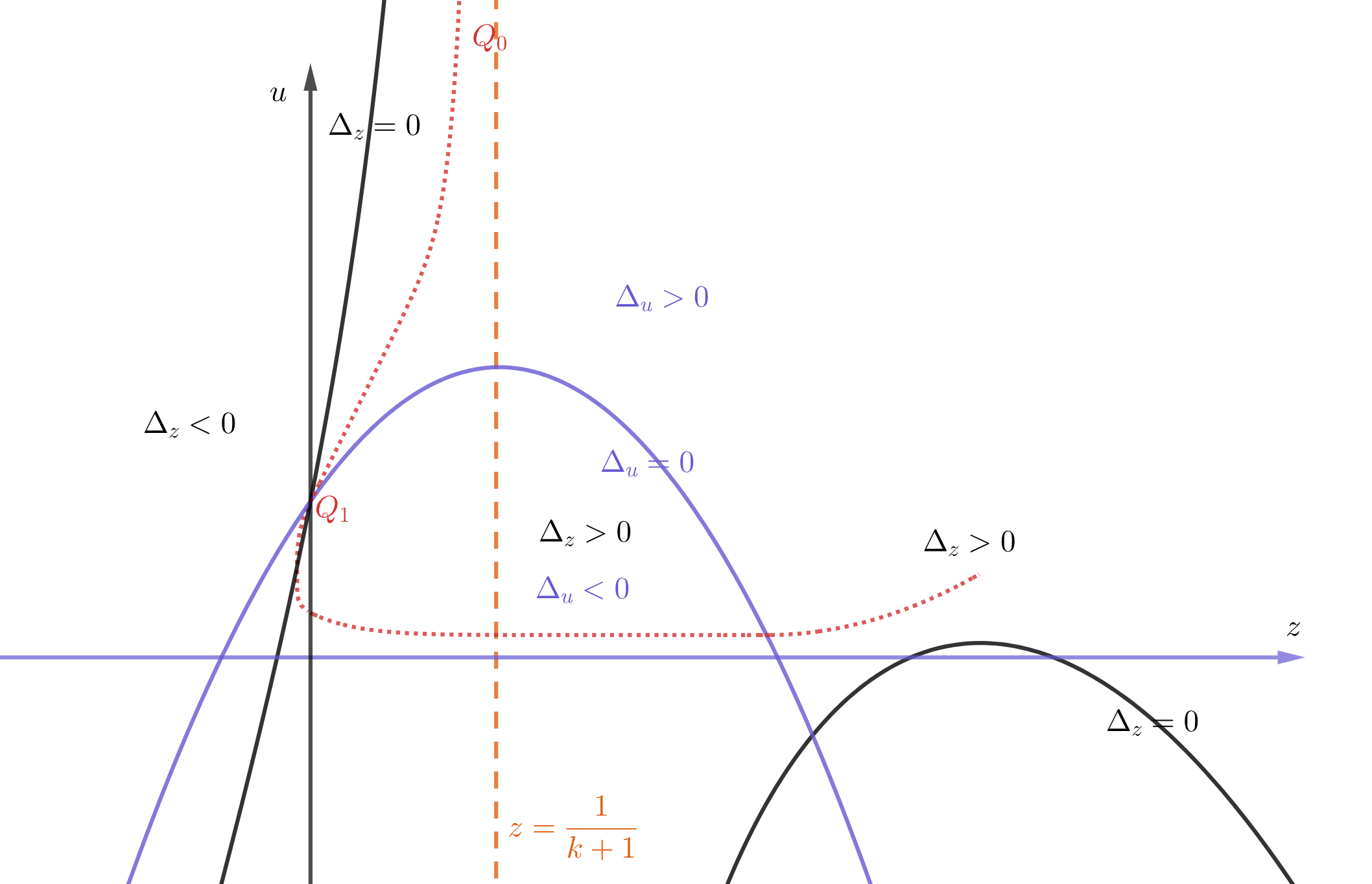
Figure 2. Phase portrait for the $z-u$ system, with $m=1.5,\ell=1.21$ and $k=3$.

We rewrite (3.11) as (if $u$ is a function of $z$)

(3.25) $$\frac{\mathrm{d}u}{\mathrm{d}z}=\frac{\Delta_{u}(z,u)}{\Delta_{z}(z,u)}=\frac{2u[u+f(z)+kz(1-z)]}{((k+1)z-1)u+(z-1)f(z)}\Leftrightarrow\mathcal{L}(u)(z)=0,$$

where

(3.26) $$\Delta_{u}(z,u)=2u[u+f(z)+kz(1-z)],\qquad\Delta_{z}(z,u)=((k+1)z-1)u+(z-1)f(z),$$

(3.27) $$\mathcal{L}(u)(z):=-\Delta_{z}(z,u){\mathrm{d}u}/{\mathrm{d}z}+\Delta_{u}(z,u).$$

For further usage, we solve $\Delta_{u}=0$ and $\Delta_{z}=0$. The solutions to $\Delta_{u}=0$ are $u=0$ and the purple curve

(3.28) $$u_{\text{p}}(z)=-f(z)-kz(1-z)=(k-B)z^{2}+(A-k)z+\varepsilon;$$

the solution to $\Delta_{z}=0$ is the black curve

(3.29) $$u_{\text{b}}(z)=-\frac{(1-z)f(z)}{1-(k+1)z}=\frac{\varepsilon+(A-\varepsilon)z-(A+B)z^{2}+Bz^{3}}{1-(k+1)z}.$$

Now we prove that the change-of-variables mapping $\Psi$ defined in (3.14) is a bijection in the regions that we are interested in. Let

(3.30) $$\mathcal{R}_{0} =\left\{(Z,v):0<v<1,0<Zv<1\right\},$$

(3.31) $$\mathcal{D}_{0} =\left\{(z,u):u>0,z<1\right\}.$$

Lemma 3.8.

The map $\Psi:\mathcal{R}_{0}\to\mathcal{D}_{0}$ is a bijection.

Proof.

We first show that $\Psi(\mathcal{R}_{0})\subset\mathcal{D}_{0}$. Let $(Z,v)\in\mathcal{R}_{0}$ and $(z,u)=\Psi(Z,v)$. Then $Z>0$, $v>0$, $1-v^{2}>0$, $1-vZ>0$ and

$$1-z=\frac{(\gamma+1)v(1-vZ)}{Z(1-v^{2})}>0,\quad u=\frac{(\gamma+1)^{2}(1-vZ)^{2}}{(1-v^{2})Z^{2}}>0,$$

thus $(z,u)\in\mathcal{D}_{0}$. Hence $\Psi(\mathcal{R}_{0})\subset\mathcal{D}_{0}$. Next we show that $\Theta(\mathcal{D}_{0})\subset\mathcal{R}_{0}$. Let $(z,u)\in\mathcal{D}_{0}$ and $(Z,v)=\Theta(z,u)$, then $u>0$, $1-z>0$, $1-z<\sqrt{u+(1-z)^{2}}$, thus $0<v<1$, $Z>0$, $Zv=\frac{1-z}{\frac{u}{1+\gamma}+1-z}<1$, and $(Z,v)\in\mathcal{R}_{0}$. Hence $\Theta(\mathcal{D}_{0})\subset\mathcal{R}_{0}$. Finally, it is direct to check that $\Theta(\Psi(Z,v))=(Z,v)$ for all $(Z,v)\in\mathcal{R}_{0}$ and $\Psi(\Theta(z,u))=(z,u)$ for all $(z,u)\in\mathcal{D}_{0}$. Therefore, $\Psi:\mathcal{R}_{0}\to\mathcal{D}_{0}$ is a bijection. ∎

Remark 3.9.

We define

$$\mathcal{N}(z,u)={\left[u+(1-z)^{2}\right]\left[u+(1+\gamma)(1-z)\right]}/{u}\in C^{\infty}(\mathcal{D}_{0}).$$

Then (3.23) and (3.24) become(with $(z,u)=\Psi(Z,v)=(\Psi_{z},\Psi_{u})$)

(3.32) $$\frac{\partial\Psi_{z}}{\partial Z}\Delta_{Z}+\frac{\partial\Psi_{z}}{\partial v}\Delta_{v}=\frac{-\Delta_{z}(z,u)}{\mathcal{N}(z,u)},$$

(3.33) $$\frac{\partial\Psi_{u}}{\partial Z}\Delta_{Z}+\frac{\partial\Psi_{u}}{\partial v}\Delta_{v}=\frac{-\Delta_{u}(z,u)}{\mathcal{N}(z,u)}.$$

If $(z,u)$ solves (3.11), let $(Z,v)=\Theta(z,u)$, then $(z,u)=\Psi(Z,v)$ and

$$0= \Delta_{z}\mathrm{d}u-\Delta_{u}\mathrm{d}z=\Delta_{z}\left(\frac{\partial\Psi_{u}}{\partial Z}\mathrm{d}Z+\frac{\partial\Psi_{u}}{\partial v}\mathrm{d}v\right)-\Delta_{u}\left(\frac{\partial\Psi_{z}}{\partial Z}\mathrm{d}Z+\frac{\partial\Psi_{z}}{\partial v}\mathrm{d}v\right)$$

$$= -\mathcal{N}\left(\frac{\partial\Psi_{z}}{\partial Z}\Delta_{Z}+\frac{\partial\Psi_{z}}{\partial v}\Delta_{v}\right)\left(\frac{\partial\Psi_{u}}{\partial Z}\mathrm{d}Z+\frac{\partial\Psi_{u}}{\partial v}\mathrm{d}v\right)$$

$$+\mathcal{N}\left(\frac{\partial\Psi_{u}}{\partial Z}\Delta_{Z}+\frac{\partial\Psi_{u}}{\partial v}\Delta_{v}\right)\left(\frac{\partial\Psi_{z}}{\partial Z}\mathrm{d}Z+\frac{\partial\Psi_{z}}{\partial v}\mathrm{d}v\right)$$

$$= \mathcal{N}\left(\frac{\partial\Psi_{z}}{\partial v}\frac{\partial\Psi_{u}}{\partial Z}-\frac{\partial\Psi_{z}}{\partial Z}\frac{\partial\Psi_{u}}{\partial v}\right)(\Delta_{Z}\mathrm{d}v-\Delta_{v}\mathrm{d}Z).$$

By (3.18) and (3.19), we have

$$\frac{\partial\Psi_{z}}{\partial v}\frac{\partial\Psi_{u}}{\partial Z}-\frac{\partial\Psi_{z}}{\partial Z}\frac{\partial\Psi_{u}}{\partial v}=\frac{2(1+\gamma)^{3}(1-Zv)^{2}}{Z^{4}(1-v^{2})^{3}}>0\quad\text{in}\ \mathcal{R}_{0}.$$

We also have $\mathcal{N}(z,u)>0$ in $\mathcal{D}_{0}$. Thus, $\Delta_{Z}\mathrm{d}v-\Delta_{v}\mathrm{d}Z=0$.

Let

(3.34) $$\mathcal{R}_{1} =\left\{(Z,v):v\in(0,v_{1}),Z\in\left(\frac{(\gamma+1)v}{1+\gamma v^{2}},\frac{\sqrt{\ell}v+1}{v+\sqrt{\ell}}\right)=(Z_{\text{b}}(v),Z_{g}(v))\right\},$$

(3.35) $$\mathcal{R}_{2} =\left\{(Z,v):v\in(v_{1},1),Z\in\left(\frac{\sqrt{\ell}v+1}{v+\sqrt{\ell}},\frac{(\gamma+1)v}{1+\gamma v^{2}}\right)=(Z_{g}(v),Z_{\text{b}}(v))\right\}.$$

Then we have

(3.36) $$\mathcal{R}_{1}=\left\{(Z,v)\in\mathcal{R}_{0}:\Delta_{v}(Z,v)>0,\ \Delta_{Z}(Z,v)>0\right\}\subset\left\{(Z,v)\in\mathcal{R}_{0}:v<Z\right\},$$

(3.37) $$\mathcal{R}_{2}=\left\{(Z,v)\in\mathcal{R}_{0}:\Delta_{v}(Z,v)<0,\ \Delta_{Z}(Z,v)<0,\ v<Z\right\}.$$

Let $\mathcal{D}_{i}=\Theta^{-1}(\mathcal{R}_{i})$. Then $\Psi:\mathcal{R}_{i}\to\mathcal{D}_{i}$ is a bijection for $i=1,2$, and (here $\chi(v,Z)=v-Z$)

$$\mathcal{D}_{1}=\left\{(z,u)\in\mathcal{D}_{0}:\Delta_{v}(\Theta(z,u))>0,\ \Delta_{Z}(\Theta(z,u))>0\right\},$$

$$\mathcal{D}_{2}=\left\{(z,u)\in\mathcal{D}_{0}:\Delta_{v}(\Theta(z,u))<0,\ \Delta_{Z}(\Theta(z,u))<0,\ \chi(\Theta(z,u))<0\right\}.$$

Now we need to evaluate $\Delta_{v}$ and $\Delta_{Z}$ in $(z,u)$. Let $(z,u)\in\mathcal{D}_{0}$ and $(Z,v)=\Theta(z,u)\in\mathcal{R}_{0}$. Then by (3.14), (3.20), (3.21) and (3.22), we get

(3.38) $$\Delta_{v}(Z,v) =\frac{k(1-v^{2})}{1+\gamma}\left[Z(1-v^{2})-(1+\gamma)v(1-Zv)\right]=\frac{k(1-v^{2})^{2}Z}{1+\gamma}z,$$

(3.39) $$\Delta_{Z}(Z,v) =Z\left[(1-Zv)^{2}-\ell(v-Z)^{2}\right]=\frac{Zu^{2}\left[u+(1-z)^{2}-\ell(z+\gamma)^{2}\right]}{\left[u+(1-z)^{2}\right]\left[u+(1+\gamma)(1-z)\right]^{2}}.$$

Therefore, we obtain (as $u>0$, $1-z>0$, $Z>0$, $0<v<1$, $k>0$, $\gamma>0$)

$$\mathcal{D}_{1}=\left\{(z,u)\in\mathcal{D}_{0}:z>0,\ u+(1-z)^{2}-\ell(z+\gamma)^{2}>0\right\},$$

$$\mathcal{D}_{2}=\left\{(z,u)\in\mathcal{D}_{0}:z<0,\ u+(1-z)^{2}-\ell(z+\gamma)^{2}<0,\ z+\gamma>0\right\}.$$

Let

(3.40) $$u_{g}(z) =\ell(z+\gamma)^{2}-(1-z)^{2}=\ell\gamma^{2}-1+2(1+\ell\gamma)z+(\ell-1)z^{2},$$

then $u_{g}(z)=(\ell-1)(z-z_{g})(z-z_{g}^{-})$ with

$$z_{g}:=\frac{1-\sqrt{\ell}\gamma}{\sqrt{\ell}+1},\quad z_{g}^{-}:=-\frac{1+\sqrt{\ell}\gamma}{\sqrt{\ell}-1},\quad z_{g}^{-}<-\gamma<z_{g}<0.$$

Thus, we can write $\mathcal{D}_{1},\mathcal{D}_{2}$ as

$$\mathcal{D}_{1}=\left\{(z,u):u>u_{g}(z),\ 0<z<1\right\},\quad\mathcal{D}_{2}=\left\{(z,u):0<u<u_{g}(z),\ z_{g}<z<0\right\}.$$

Similarly, let

$$\mathcal{R}_{2}^{+}:=\left\{(Z,v):v\in(v_{1},1),Z=\frac{\sqrt{\ell}v+1}{v+\sqrt{\ell}}=Z_{g}(v)\right\}.$$

Then we have

$$\mathcal{R}_{2}^{+}=\left\{(Z,v)\in\mathcal{R}_{0}:\Delta_{v}(Z,v)<0,\ \Delta_{Z}(Z,v)=0,\ v<Z\right\}.$$

Let $\mathcal{D}_{2}^{+}=\Theta^{-1}(\mathcal{R}_{2}^{+})$. Then $\Psi:\mathcal{R}_{2}^{+}\to\mathcal{D}_{2}^{+}$ is a bijection and

$$\mathcal{D}_{2}^{+} =\left\{(z,u)\in\mathcal{D}_{0}:\Delta_{v}(\Theta(z,u))<0,\ \Delta_{Z}(\Theta(z,u))=0,\ \chi(\Theta(z,u))<0\right\}$$

$$=\left\{(z,u)\in\mathcal{D}_{0}:z<0,\ u+(1-z)^{2}-\ell(z+\gamma)^{2}=0,\ z+\gamma>0\right\}$$

$$=\left\{(z,u):u=u_{g}(z),\ z_{g}<z<0\right\}.$$

3.3. The $Q_{0}-Q_{1}$ curve

Here we prove that the $P_{0}-P_{1}$ solution curve $v_{F}$ of the $Z-v$ ODE (3.2) corresponds to a solution curve $u_{F}$ of the $z-u$ ODE (3.25) that connects $Q_{0}$ to $Q_{1}$, where $Q_{0}=\left(z=\frac{1}{k+1},u=+\infty\right)$, see the dashed red curve in Figure 2 connecting $Q_{0}$ and $Q_{1}$.

Lemma 3.10.

It holds that

(3.41) $$\lim_{Z\downarrow 0}\Psi_{z}(Z,v_{F}(Z))=\frac{1}{k+1},\qquad\lim_{Z\downarrow 0}\Psi_{u}(Z,v_{F}(Z))=+\infty,$$

(3.42) $$\qquad\qquad\lim_{Z\downarrow 0}\frac{1}{Z}\frac{\mathrm{d}}{\mathrm{d}Z}\Psi_{z}(Z,v_{F}(Z))<0.$$

Proof.

Since $v_{F}$ has the asymptotic behavior (3.9), we compute

$$\lim_{Z\downarrow 0}\Psi_{u}(Z,v_{F}(Z)) =\lim_{Z\downarrow 0}\frac{(1+\gamma)^{2}\big{(}1-Zv_{F}(Z)\big{)}^{2}}{Z^{2}\big{(}1-v_{F}(Z)^{2}\big{)}}=(1+\gamma)^{2}\lim_{Z\downarrow 0}\frac{1}{Z^{2}}=+\infty,$$

$$\lim_{Z\downarrow 0}\Psi_{z}(Z,v_{F}(Z)) =\lim_{Z\downarrow 0}\frac{1+\gamma v_{F}(Z)^{2}-(1+\gamma)\frac{v_{F}(Z)}{Z}}{1-v_{F}(Z)^{2}}=1-(1+\gamma)\frac{m}{k+1}=\frac{1}{k+1}.$$

Also, as $Z\downarrow 0$, we have

$$\frac{1}{k+1}-\Psi_{z}(Z,v_{F}(Z))=\frac{1}{k+1}-\frac{1+\gamma v_{F}(Z)^{2}-(1+\gamma)\frac{v_{F}(Z)}{Z}}{1-v_{F}(Z)^{2}}$$

$$=\frac{(1+\gamma)\frac{v_{F}(Z)}{Z}+\frac{1}{k+1}-1-\left(\gamma+\frac{1}{k+1}\right)v_{F}(Z)^{2}}{1-v_{F}(Z)^{2}}$$

$$=\frac{(1+\gamma)\left(\frac{m}{k+1}+\phi_{1}Z^{2}+O(Z^{4})\right)-\frac{k}{k+1}-\left(\gamma+\frac{1}{k+1}\right)\left(\frac{m^{2}}{(k+1)^{2}}Z^{2}+O(Z^{4})\right)}{1-v_{F}(Z)^{2}}$$

$$=\left[(1+\gamma)\phi_{1}-\left(\gamma+\frac{1}{k+1}\right)\frac{m^{2}}{(k+1)^{2}}\right]Z^{2}+O(Z^{4}).$$

As $\frac{v_{F}(Z)}{Z}$ is real analytic in ${Z}$, so is $\Psi_{z}(Z,v_{F}(Z))$. Thus, for (3.42), it suffices to show

(3.43) $$\phi_{1}>\frac{1}{1+\gamma}\left(\gamma+\frac{1}{k+1}\right)\frac{m^{2}}{(k+1)^{2}}=\frac{k^{2}\left[(k+1)\gamma+1\right]}{(k+1)^{3}(\gamma+1)^{3}}.$$

By (3.6) and $m=k/(\gamma+1)$, we compute

$$(k+3)\phi_{1} =\ell\frac{k}{(k+1)(\gamma+1)}+\left(k-2\ell+2-\frac{2k}{\gamma+1}\right)\frac{k^{2}}{(k+1)^{2}(\gamma+1)^{2}}+\frac{k^{3}(k+\ell)}{(k+1)^{3}(\gamma+1)^{3}}$$

$$=\frac{k\Big{[}\ell(k+1)^{2}(\gamma+1)^{2}+k(k+1)\left[(k+2-2\ell)(\gamma+1)-2k\right]+k^{2}(k+\ell)\Big{]}}{(k+1)^{3}(\gamma+1)^{3}}$$

$$=\frac{k\Big{[}\ell(k+1)^{2}\gamma^{2}+(k+1)(k^{2}+2k+2\ell)\gamma+k^{2}+2k+\ell\Big{]}}{(k+1)^{3}(\gamma+1)^{3}}$$

$$=\frac{k[(k+1)\gamma+1]\Big{[}\ell(k+1)\gamma+k^{2}+2k+\ell\Big{]}}{(k+1)^{3}(\gamma+1)^{3}}.$$

Therefore, we arrive at

$$\phi_{1}-\frac{k^{2}\left[(k+1)\gamma+1\right]}{(k+1)^{3}(\gamma+1)^{3}}=\frac{k\left[(k+1)\gamma+1\right]\big{[}\ell(k+1)\gamma+k^{2}+2k+\ell-k(k+3)\big{]}}{(k+3)(k+1)^{3}(\gamma+1)^{3}}$$

$$=\frac{k\left[(k+1)\gamma+1\right]\big{[}\ell(k+1)\gamma+\ell-k\big{]}}{(k+3)(k+1)^{3}(\gamma+1)^{3}}=\frac{k\left[(k+1)\gamma+1\right]\big{[}(\ell\gamma-1)k+\ell+\ell\gamma\big{]}}{(k+3)(k+1)^{3}(\gamma+1)^{3}}>0,$$

where we have used $\ell\gamma>\ell\cdot\frac{1}{\sqrt{\ell}}=\sqrt{\ell}>1$. This proves (3.43) and thus (3.42). ∎

Lemma 3.11.

It holds that

(3.44) $$u_{\text{p}}(z)<u_{g}(z)<u_{\text{b}}(z)\quad\forall\ z\in\left(0,\frac{1}{k+1}\right),$$

where $u_{p},u_{b},u_{g}$ are given by (3.28), (3.29) and (3.40) respectively.

Proof.

For $z\in\mathbb{R}$, we compute (using (3.12))

(3.45) $$u_{\text{p}}(z)-u_{g}(z)=(k-B-\ell+1)z^{2}+(A-k-2(1+\ell\gamma))z=-kz(z+\gamma),$$

and

$$u_{\text{b}}(z)-u_{g}(z) =\frac{\varepsilon+(A-\varepsilon)z-(A+B)z^{2}+Bz^{3}}{1-(k+1)z}-\big{(}\varepsilon+2(1+\ell\gamma)z+(\ell-1)z^{2}\big{)}$$

$$=\frac{k\gamma(\ell\gamma-1)z+k(2\ell\gamma+\gamma-1)z^{2}+k(\ell+1)z^{3}}{1-(k+1)z},$$

which gives (3.44) by using $\ell\gamma-1>0$ and $2\ell\gamma+\gamma-1=\ell\gamma-1+\ell\gamma+\gamma>0$. ∎

We consider the domain

(3.46) $$\mathcal{D}_{1}^{\prime}= \left\{(z,u):u_{g}(z)<u<u_{\text{b}}(z),\quad z\in\left(0,\frac{1}{k+1}\right)\right\}$$

$$= \left\{(z,u)\in\mathcal{D}_{1}:\Delta_{z}(z,u)>0,\quad z\in\left(0,\frac{1}{k+1}\right)\right\}.$$

The main result of this subsection is stated as follows.

Proposition 3.12.

The unique $P_{0}-P_{1}$ smooth solution $v_{F}(Z)\ (0<Z<Z_{1})$ to the $Z-v$ ODE (3.2) is mapped through $\Psi$ to a smooth solution $u=u_{F}(z)\ \left(0<z<\frac{1}{k+1}\right)$ of the $z-u$ ODE (3.25) with the following properties:

• $u_{F}$ is a strictly increasing function with respect to $z\in\left(0,\frac{1}{k+1}\right)$;

• we have

  (3.47) $$u_{\text{p}}(z)<u_{g}(z)<u_{F}(z)<u_{\text{b}}(z),\quad\Delta_{z}(z,u_{F}(z))>0\quad\forall\ z\in\left(0,\frac{1}{k+1}\right);$$

• $\lim_{z\downarrow 0}u_{F}(z)=\varepsilon$, $\lim_{z\uparrow 1/(k+1)}u_{F}(z)=+\infty$.

Moreover, we have

(3.48) $$\Theta_{v}(z,u_{F}(z))=v_{F}\big{(}\Theta_{Z}(z,u_{F}(z))\big{)}\quad\forall\ z\in\left(0,\frac{1}{k+1}\right).$$

Proof.

By (3.7), (3.36) and $Z_{1}\in(0,1)$, we have $(Z,v_{F}(Z))\in\mathcal{R}_{1}$ for $Z\in(0,Z_{1})$, and then

$$(z(Z),u(Z)):=\Psi(Z,v_{F}(Z))\in\mathcal{D}_{1}\subset\mathcal{D}_{0},\qquad\forall\ Z\in(0,Z_{1}).$$

By (3.16), (3.17), (3.32) and (3.33), we get

$$\frac{\mathrm{d}z}{\mathrm{d}Z}=\frac{-\Delta_{z}(z,u)}{\Delta_{Z}(Z,v_{F})\mathcal{N}(z,u)},\quad\frac{\mathrm{d}u}{\mathrm{d}Z}=\frac{-\Delta_{u}(z,u)}{\Delta_{Z}(Z,v_{F})\mathcal{N}(z,u)}.$$

Let $\eta_{1}(Z):=[\Delta_{Z}(Z,v_{F}(Z))\mathcal{N}(z(Z),u(Z))]^{-1}$. As $\Delta_{Z}>0$ in $\mathcal{R}_{1}$ and $\mathcal{N}>0$ in $\mathcal{D}_{0}$, we have

(3.49) $$\frac{\mathrm{d}z}{\mathrm{d}Z}=-\eta_{1}(Z)\Delta_{z}(z,u),\quad\frac{\mathrm{d}u}{\mathrm{d}Z}=-\eta_{1}(Z)\Delta_{u}(z,u),\quad\eta_{1}(Z)>0\quad\text{for}\ Z\in(0,Z_{1}).$$

According to Lemma 3.10, there exists a small $\Upsilon_{0}>0$ such that for all $Z\in(0,\Upsilon_{0})$, $\frac{\mathrm{d}z}{\mathrm{d}Z}<0$ and $\lim_{Z\downarrow 0}z(Z)=\frac{1}{k+1}$. Then $0<z(Z)<\frac{1}{k+1}$ for all $Z\in(0,\Upsilon_{0})$. By (3.49), we have $\Delta_{z}(z(Z),u(Z))>0$ for all $Z\in(0,\Upsilon_{0})$. Now we claim that

$$\Delta_{z}(z(Z),u(Z))>0\quad\forall\ Z\in(0,Z_{1}).$$

Otherwise, there exists $Z_{2}\in(0,Z_{1})$ such that $\Delta_{z}(z(Z),u(Z))>0$ for all $Z\in(0,Z_{2})$ and $\Delta_{z}(z(Z_{2}),u(Z_{2}))=0$. Then $\frac{\mathrm{d}}{\mathrm{d}Z}\Delta_{z}(z,u)|_{Z=Z_{2}}\leq 0$. By (3.49), we have $\frac{\mathrm{d}z}{\mathrm{d}Z}<0$ for all $Z\in(0,Z_{2})$, $\frac{\mathrm{d}z}{\mathrm{d}Z}|_{Z=Z_{2}}=0$ and $0<z(Z)<\frac{1}{k+1}$ for all $Z\in(0,Z_{2}]$. By $(z(Z),u(Z))\in\mathcal{D}_{1}$ and Lemma 3.11, we have $u(Z)>u_{g}(z(Z))>u_{\text{p}}(z(Z))$, $u(Z)>0$ and $\Delta_{u}(z(Z),u(Z))=2u(Z)(u(Z)-u_{\text{p}}(z(Z)))>0$ for all $Z\in(0,Z_{2}]$. Then by (3.49) again, we have $\frac{\mathrm{d}u}{\mathrm{d}Z}<0$ for all $Z\in(0,Z_{2}]$. As $(k+1)z-1<0$ and $\frac{\mathrm{d}u}{\mathrm{d}Z}<0$ for $z=Z_{2}$, we also have

$$\frac{\mathrm{d}}{\mathrm{d}Z}\Delta_{z}(z,u)\Big{|}_{Z=Z_{2}} =\left(\partial_{z}\Delta_{z}(z,u)\frac{\mathrm{d}z}{\mathrm{d}Z}+\partial_{u}\Delta_{z}(z,u)\frac{\mathrm{d}u}{\mathrm{d}Z}\right)\Big{|}_{Z=Z_{2}}=\partial_{u}\Delta_{z}(z,u)\frac{\mathrm{d}u}{\mathrm{d}Z}\Big{|}_{Z=Z_{2}}$$

$$=((k+1)z-1)\frac{\mathrm{d}u}{\mathrm{d}Z}\Big{|}_{Z=Z_{2}}>0,$$

which reaches a contradiction. So, $\Delta_{z}(z(Z),u(Z))>0$ for all $Z\in(0,Z_{1})$.

By $(z(Z),u(Z))\in\mathcal{D}_{1}$ and Lemma 3.11, we have $u(Z)>u_{g}(z(Z))>u_{\text{p}}(z(Z))$, and

$$\Delta_{u}(z(Z),u(Z))=2u(Z)\big{(}u(Z)-u_{\text{p}}(z(Z))\big{)}>0\quad\forall\ Z\in(0,Z_{1}).$$

Therefore, we conclude by (3.49) that $\frac{\mathrm{d}z}{\mathrm{d}Z}<0$ and $\frac{\mathrm{d}u}{\mathrm{d}Z}<0$. Hence, both $z(Z)$ and $u(Z)$ are strictly decreasing for $Z\in(0,Z_{1})$. Thus, $0<z(Z)<\frac{1}{k+1}$ for all $Z\in(0,Z_{1})$, which along with $(z(Z),u(Z))\in\mathcal{D}_{1}$, $\Delta_{z}(z(Z),u(Z))>0$ for all $Z\in(0,Z_{1})$ implies $(z(Z),u(Z))\in\mathcal{D}_{1}^{\prime}$ for all $Z\in(0,Z_{1})$. By Lemma 3.10, we have

(3.50) $$\lim_{Z\downarrow 0}z(Z)=\lim_{Z\downarrow 0}\Psi_{z}(Z,v_{F}(Z))=\frac{1}{k+1},\quad\lim_{Z\downarrow 0}u(Z)=\lim_{Z\downarrow 0}\Psi_{u}(Z,v_{F}(Z))=+\infty.$$

By $\Psi(Z_{1},v_{1})=Q_{1}=(0,\varepsilon)$ and (3.8), we have

(3.51) $$\lim_{Z\uparrow Z_{1}}(z(Z),u(Z))=\lim_{Z\uparrow Z_{1}}\Psi(Z,v_{F}(Z))=Q_{1}=(0,\varepsilon).$$

Let $Z(z)\ (0<z<\frac{1}{k+1})$ denote the inverse function of $z=z(Z)\ (0<Z<Z_{1})$, and we define

$$u_{F}(z)=u(Z(z))\quad\forall\ z\in\left(0,\frac{1}{k+1}\right).$$

We check that $u_{F}$ is a desired solution to the $z-u$ ODE connecting $Q_{0}$ and $Q_{1}$. Since $z(Z)$ and $u(Z)$ are strictly decreasing, $u_{F}$ is also strictly increasing; by (3.49), we have

$$\frac{\mathrm{d}u_{F}}{\mathrm{d}z}=\frac{\mathrm{d}u/\mathrm{d}Z}{\mathrm{d}z/\mathrm{d}Z}=\frac{\Delta_{u}(z,u_{F}(z))}{\Delta_{z}(z,u_{F}(z))};$$

by $(z,u_{F}(z))=(z,u)(Z(z))\in\mathcal{D}_{1}^{\prime}$, we have $u_{g}(z)<u_{F}(z)<u_{\text{b}}(z)$ and $\Delta_{z}(z,u_{F}(z))>0$ for all $z\in(0,1/(k+1))$; by (3.50) and (3.51), we have

$$\lim_{z\downarrow 0}u_{F}(z)=\varepsilon,\quad\lim_{z\uparrow 1/(k+1)}u_{F}(z)=+\infty.$$

Finally, by the definition, we have $(z(Z),u(Z))=\Psi\big{(}Z,v_{F}(Z)\big{)}\in\mathcal{D}_{0}$ for all $Z\in(0,Z_{1})$, hence by Lemma 3.8 and the definition of $u_{F}$, we have $\big{(}Z,v_{F}(Z)\big{)}=\Theta\big{(}z(Z),u_{F}(Z)\big{)}$ for all $Z\in(0,Z_{1})$, and thus $\Theta_{v}\big{(}z(Z),u_{F}(z(Z))\big{)}=v_{F}\Big{(}\Theta_{Z}\big{(}z(Z),u_{F}(z(Z))\big{)}\Big{)}$ for all $Z\in(0,Z_{1})$. Now since $z(Z)$ is a bijection from $Z\in(0,Z_{1})$ onto $z\in(0,1/(k+1))$, we deduce (3.48). ∎

4. Local smooth solution around the sonic point

In this section, we construct a smooth local solution $u_{L}$ to the $z-u$ ODE (3.25) passing through the sonic point $Q_{1}(z=0,u=\varepsilon)$. In Subsection 4.1, we first show that all smooth solutions to the $z-u$ ODE (3.25) passing through $Q_{1}$ has two possible slopes at $Q_{1}$, and we determine the desired slope of $u_{L}$ at $Q_{1}$ using the information of $u_{F}$ constructed in the previous section. In Subsection 4.2, we show that the ratio $R>1$ of the eigenvalues of the linearized system of (3.25) at $Q_{1}$ plays a very important role in the construction of $u_{L}$. In Subsection 4.3, we use the power series method to construct $u_{L}$, which can be transformed by $\Theta$ to a local solution $v_{L}(Z)$ of the $Z-v$ ODE passing through $P_{1}$.

Let’s recall the notations introduced in last section:

$$\varepsilon=\ell\gamma^{2}-1,\quad A=k+2-(k-2\ell)\gamma,\quad B=2k+1-\ell,\quad\gamma=k/m-1.$$

4.1. Slope at $Q_{1}$

Assume that $u(z)$ is a local smooth solution of (3.25) passing through $Q_{1}$. Let $a_{1}=u^{\prime}(0)$. By L’Hôpital’s rule, we have

$$a_{1}=\frac{\mathrm{d}u}{\mathrm{d}z}\Big{|}_{z=0}=\frac{\partial_{z}\Delta_{u}(Q_{1})+\partial_{u}\Delta_{u}(Q_{1})a_{1}}{\partial_{z}\Delta_{z}(Q_{1})+\partial_{u}\Delta_{z}(Q_{1})a_{1}}.$$

We define

(4.1) $$\tilde{c}_{1}: =\partial_{u}\Delta_{u}(Q_{1})=2\varepsilon,\qquad\qquad\tilde{c}_{2}:=\partial_{u}\Delta_{z}(Q_{1})=-1,$$

$$\tilde{c}_{3}: =\partial_{z}\Delta_{u}(Q_{1})=2\varepsilon(k-A),\quad\tilde{c}_{4}:=\partial_{z}\Delta_{z}(Q_{1})=k\varepsilon+A.$$

Then $a_{1}$ satisfies the quadratic equation $-\tilde{c}_{2}a_{1}^{2}+(\tilde{c}_{1}-\tilde{c}_{4})a_{1}+\tilde{c}_{3}=0$, i.e.,

(4.2) $$p_{0}(a_{1}):=a_{1}^{2}-((k-2)\varepsilon+A)a_{1}+2(k-A)\varepsilon=0.$$

Since

$$p_{0}(2(1+\ell\gamma))=\big{(}2(1+\ell\gamma)\big{)}^{2}-2\big{(}(k-2)\varepsilon+A\big{)}(1+\ell\gamma)+2(k-A)\varepsilon$$

$$= 4(1+\ell\gamma)^{2}-2(1+\ell\gamma)\big{(}k(\ell\gamma^{2}-\gamma)+4-2\ell\gamma^{2}+2\ell\gamma\big{)}+2k\gamma(\ell\gamma^{2}-1)-4(1+\ell\gamma)(\ell\gamma^{2}-1)$$

$$= 2k\ell\gamma^{3}(1-\ell)<0,$$

we know that the quadratic polynomial $p_{0}$ has two real roots, where the larger one is greater than $2(1+\ell\gamma)>4>0$ and the smaller one is smaller than $2(1+\ell\gamma)$, and the discriminant of $p_{0}$ is $(\tilde{c}_{1}-\tilde{c}_{4})^{2}+4\tilde{c}_{2}\tilde{c}_{3}>0$. Similarly, we have

(4.3) $$p_{0}({2}(1+s\gamma)) =2(2s+k)(s-\ell)\gamma^{2}+2(k-2\ell-(k-2)s)\ell\gamma^{3},$$

whose proof will be delayed until we prove Lemma A.3.

We claim that $a_{1}$ must be the larger root of $p_{0}$. In fact, as $u_{F}(z)>u_{g}(z)$ for $z\in(0,1/(k+1))$, $u_{F}(0)=\varepsilon=\ell\gamma^{2}-1=u_{g}(0)$, we have $a_{1}=u^{\prime}(0)=u_{F}^{\prime}(0)\geq u_{g}^{\prime}(0)=2(1+\ell\gamma)$. Thus

(4.4) $$a_{1}>2(1+\ell\gamma)>4,$$

(4.5) $$a_{1}=\frac{\tilde{c}_{4}-\tilde{c}_{1}+\sqrt{(\tilde{c}_{1}-\tilde{c}_{4})^{2}+4\tilde{c}_{2}\tilde{c}_{3}}}{2}=\frac{(k-2)\varepsilon+A+\sqrt{\big{(}(k-2)\varepsilon+A\big{)}^{2}-8(k-A)\varepsilon}}{2}.$$

4.2. Eigenvalues

We start with some heuristic discussions. Consider the ODE

(4.6) $$\frac{\mathrm{d}y}{\mathrm{d}x}=\frac{a_{11}y+a_{12}x+R_{1}(x,y)}{a_{21}y+a_{22}x+R_{2}(x,y)},$$

where $a_{11},a_{12},a_{21},a_{22}$ are constants and $R_{1},R_{2}$ are smooth functions with $R_{1}(x,y)=O(x^{2})+O(y^{2})$, $R_{2}(x,y)=O(x^{2})+O(y^{2})$ as $(x,y)\to(0,0)$. We introduce a time variable $\tau$ such that $\frac{\mathrm{d}x}{\mathrm{d}\tau}=a_{21}y+a_{22}x+R_{2}(x,y)$, then (4.6) is converted to the ODE system

(4.7) $$\frac{\mathrm{d}}{\mathrm{d}\tau}\begin{pmatrix}y\\ x\end{pmatrix}=\begin{pmatrix}a_{11}&a_{12}\\ a_{21}&a_{22}\end{pmatrix}\begin{pmatrix}y\\ x\end{pmatrix}+\begin{pmatrix}R_{1}(x,y)\\ R_{2}(x,y)\end{pmatrix}.$$

Clearly, (4.7) has a trivial solution $(x,y)=(0,0)$. Near this equilibrium, the behavior of the solutions of (4.7) can be approximated by the linear ODE system

(4.8) $$\frac{\mathrm{d}}{\mathrm{d}\tau}\begin{pmatrix}y\\ x\end{pmatrix}=\mathcal{A}\begin{pmatrix}y\\ x\end{pmatrix}=\begin{pmatrix}a_{11}&a_{12}\\ a_{21}&a_{22}\end{pmatrix}\begin{pmatrix}y\\ x\end{pmatrix}.$$

We assume that the matrix $\mathcal{A}$ has two distinct positive eigenvalues $\lambda_{1}>\lambda_{2}>0$ with $R=\frac{\lambda_{1}}{\lambda_{2}}\in(1,+\infty)\setminus\mathbb{Z}$. Let $\mathcal{P}$ be a $2\times 2$ matrix such that

$$\mathcal{P}\mathcal{A}\mathcal{P}^{-1}=\begin{pmatrix}\lambda_{1}&\\ &\lambda_{2}\end{pmatrix},$$

and let

(4.9) $$\begin{pmatrix}Y\\ X\end{pmatrix}=\mathcal{P}\begin{pmatrix}y\\ x\end{pmatrix},$$

then the linear ODE system (4.8) is reduced to

(4.10) $$\frac{\mathrm{d}}{\mathrm{d}\tau}\begin{pmatrix}Y\\ X\end{pmatrix}=\begin{pmatrix}\lambda_{1}&\\ &\lambda_{2}\end{pmatrix}\begin{pmatrix}Y\\ X\end{pmatrix}.$$

Thus, $Y(\tau)=Y(0)e^{\lambda_{1}\tau},X(\tau)=X(0)e^{\lambda_{2}\tau}$. We observe that the curve $\tau\mapsto(X(\tau),Y(\tau))$ gives a smooth curve in the phase space $(X,Y)$ if and only $X(0)=0$ or $Y(0)=0$, which corresponds to the solution $X\equiv 0$ or $Y\equiv 0$ respectively; and if $X(0)\neq 0$ and $Y(0)\neq 0$, the solution satisfies $Y=C_{0}X^{R}$ with some non-zero constant $C_{0}$, hence has only $C^{R}$ regularity, recalling that we assume $R=\frac{\lambda_{1}}{\lambda_{2}}\in(1,+\infty)\setminus\mathbb{Z}$.

Due to the smoothness of the change of variables (4.9), we expect that among all solutions of nonlinear ODE (4.6) passing through $(0,0)$, only two of them are smooth and any other solutions have $C^{R}$ regularity; moreover, we can select the only smooth solution of (4.6) passing through $(0,0)$ as long as we specify the slope of this solution. As a result, when we use the power series method to construct the smooth solution $y=\sum_{n=0}^{\infty}y_{n}x^{n}$ of (4.6) passing through $(0,0)$, we need to analyze the coefficients $y_{n}$ at least from $y_{0}$ to $y_{\lfloor R\rfloor+1}$, in order to distinguish it from non-smooth solutions, which are only $C^{R}$ regular.

The above heuristic discussions inspire us to consider the eigenvalues of our $z-u$ ODE (3.25) near $Q_{1}$. The linearization of (3.25) near $Q_{1}$ is

$$\frac{\mathrm{d}(u-\varepsilon)}{\mathrm{d}z}=\frac{\partial_{z}\Delta_{u}(Q_{1})z+\partial_{u}\Delta_{u}(Q_{1})(u-\varepsilon)}{\partial_{z}\Delta_{z}(Q_{1})z+\partial_{u}\Delta_{z}(Q_{1})(u-\varepsilon)},$$

whose coefficient matrix is

(4.11) $$\mathcal{A}=\begin{pmatrix}\partial_{u}\Delta_{u}(Q_{1})&\partial_{z}\Delta_{u}(Q_{1})\\ \partial_{u}\Delta_{z}(Q_{1})&\partial_{z}\Delta_{z}(Q_{1})\end{pmatrix}=\begin{pmatrix}\tilde{c}_{1}&\tilde{c}_{3}\\ \tilde{c}_{2}&\tilde{c}_{4}\end{pmatrix}=\begin{pmatrix}2\varepsilon&2\varepsilon(k-A)\\ -1&k\varepsilon+A\end{pmatrix},$$

with characteristic polynomial $\varphi_{\mathcal{A}}(\lambda)=\lambda^{2}-(\tilde{c}_{1}+\tilde{c}_{4})\lambda+\tilde{c}_{1}\tilde{c}_{4}-\tilde{c}_{2}\tilde{c}_{3}=\lambda^{2}-((k+2)\varepsilon+A)\lambda+2k\varepsilon(\varepsilon+1)$, which has two positive roots $0<\lambda_{-}<\lambda_{+}$, since $2k\varepsilon(\varepsilon+1)>0$,

$$\tilde{c}_{1}+\tilde{c}_{4} =(k+2)\varepsilon+A=(k+2)(\ell\gamma^{2}-1)+k+2-(k-2\ell)\gamma=\left[(k+2)\ell\gamma-k+2\ell\right]\gamma$$

$$>\left[(k+2)\ell\frac{1}{\sqrt{\ell}}-k+2\ell\right]\gamma=\left[k(\sqrt{\ell}-1)+2\sqrt{\ell}(1+\sqrt{\ell})\right]\gamma>0,$$

and the discriminant $(\tilde{c}_{1}-\tilde{c}_{4})^{2}+4\tilde{c}_{2}\tilde{c}_{3}>0$ (which is the same as the discriminant of $p_{0}$).

By a direct computation, we have

(4.12) $$\lambda_{\pm}=\frac{\tilde{c}_{1}+\tilde{c}_{4}\pm\sqrt{(\tilde{c}_{1}-\tilde{c}_{4})^{2}+4\tilde{c}_{2}\tilde{c}_{3}}}{2}.$$

Let $R=\frac{\lambda_{+}}{\lambda_{-}}>1$. Then we have

(4.13) $$\frac{(R+1)^{2}}{R}=\frac{(\lambda_{+}+\lambda_{-})^{2}}{\lambda_{+}\lambda_{-}}=\frac{(\tilde{c}_{1}+\tilde{c}_{4})^{2}}{\tilde{c}_{1}\tilde{c}_{4}-\tilde{c}_{2}\tilde{c}_{3}}=\frac{[(k+2)\ell\gamma-(k-2\ell)]^{2}}{2k\ell(\ell\gamma^{2}-1)}.$$

The subsequent analysis is based on the assumption $R\in(3,4)$. However, it turns out that in some circumstances, $R$ may not belong to $(3,4)$. As a consequence, we need to explore the conditions of parameters ensuring $R\in(3,4)$.

Lemma 4.1.

For each $\ell>1,k\in\mathbb{Z}_{+},\gamma>\frac{1}{\sqrt{\ell}}$, we define the ratio

(4.14) $$R=R(k,\ell,\gamma)=\frac{\lambda_{+}}{\lambda_{-}}>1.$$

Let $\mathcal{K}$ be the admissible set of $(k,\ell)$ defined by

(4.15) $$\mathcal{K}=\left\{(k,\ell)\in\mathbb{Z}_{+}\times[1,+\infty):k\leq 5\text{ or }1<\ell<\ell_{0}(k)\text{ for }k\geq 6\right\},$$

where

(4.16) $$\ell_{0}(k):=\frac{3k^{2}-8k+12-\sqrt{(3k-2)(k-6)(3k^{2}+4k+12)}}{24}\qquad\text{for}\quad k\geq 6.$$

For each $\ell>1,k\in\mathbb{Z}_{+}$, there exists $R_{\text{inf}}=R_{\text{inf}}(k,\ell)\geq 1$ such that the range of the function $\gamma\mapsto R(k,\ell,\gamma)$ is the interval $(R_{\text{inf}},+\infty)$ or $[R_{\text{inf}},+\infty)$; furthermore, $R_{\text{inf}}(k,\ell)<3$ if and only if $(k,\ell)\in\mathcal{K}$.

Remark 4.2.

The symbol $R_{\text{inf}}(k,\ell)$ stands for the infimum value of the function $\gamma\mapsto R(k,\ell,\gamma)$. We have $1<\ell_{0}(k)<k/2$ for $k>6$, $\lim_{k\to\infty}\ell_{0}(k)=1$ and $\ell_{0}(7)\approx 1.81$, $\ell_{0}(6)=3$.

Proof.

For fixed $k,\ell$, we denote the right hand side of (4.13) by $F(\gamma)$, and then

$$F^{\prime}(\gamma)=-\frac{[(k+2)-(k-2\ell)\gamma][(k+2)\ell\gamma-(k-2\ell)]}{k(\ell\gamma^{2}-1)^{2}}.$$

As $\gamma>\frac{1}{\sqrt{\ell}}$, we have $\ell\gamma>\ell\frac{1}{\sqrt{\ell}}>1$ and

$$(k+2)\ell\gamma-(k-2\ell)>(k+2)-(k-2\ell)=2+2\ell>0.$$

If $k\leq 2\ell$, then $(k+2)-(k-2\ell)\gamma>0$ and $F^{\prime}(\gamma)<0$ for $\gamma>\frac{1}{\sqrt{\ell}}$, the function $F(\gamma)$ is strictly decreasing for $\gamma>\frac{1}{\sqrt{\ell}}$, with $\lim_{\gamma\downarrow\frac{1}{\sqrt{\ell}}}F(\gamma)=+\infty$ and $\lim_{\gamma\to+\infty}F(\gamma)=\frac{(k+2)^{2}}{2k}$. Also note that the function $R\mapsto\frac{(R+1)^{2}}{R}$ is strictly increasing for $R>1$, hence the function $\gamma\mapsto R(k,\ell,\gamma)$ is strictly decreasing for $\gamma>\frac{1}{\sqrt{\ell}}$, with $\lim_{\gamma\downarrow\frac{1}{\sqrt{\ell}}}R(k,\ell,\gamma)=+\infty$ and $R_{\text{inf}}:=\lim_{\gamma\to+\infty}R(k,\ell,\gamma)\geq 1$ satisfying

(4.17) $$\frac{(R_{\text{inf}}+1)^{2}}{R_{\text{inf}}}=\frac{(k+2)^{2}}{2k}\geq 4\Longrightarrow R_{\text{inf}}=\max\left\{\frac{k}{2},\frac{2}{k}\right\}\geq 1.$$

Therefore, $R_{\text{inf}}<3$ if and only if $1\leq k\leq 5$.

If $k>2\ell$, let $\gamma_{1}=\frac{k+2}{k-2\ell}$, then $\gamma_{1}>1>\frac{1}{\sqrt{\ell}}$ and

$$(k+2)-(k-2\ell)\gamma>0,\quad F^{\prime}(\gamma)<0\quad\text{for}\ 1/\sqrt{\ell}<\gamma<\gamma_{1},$$

$$(k+2)-(k-2\ell)\gamma<0,\quad F^{\prime}(\gamma)>0\quad\text{for}\ \gamma>\gamma_{1}.$$

Thus, the function $F(\gamma)$ is strictly decreasing for $\frac{1}{\sqrt{\ell}}<\gamma\leq\gamma_{1}$, strictly increasing for $\gamma\geq\gamma_{1}$ with $\lim_{\gamma\downarrow\frac{1}{\sqrt{\ell}}}F(\gamma)=+\infty$ and

$$F(\gamma_{1})=\frac{[(k+2)\ell\gamma_{1}-(k-2\ell)]^{2}}{2k\ell(\ell\gamma_{1}^{2}-1)}=\frac{[(k+2)^{2}\ell/(k-2\ell)-(k-2\ell)]^{2}}{2k\ell(\ell(k+2)^{2}/(k-2\ell)^{2}-1)}=\frac{(k+2)^{2}\ell-(k-2\ell)^{2}}{2k\ell}.$$

Since $R\mapsto\frac{(R+1)^{2}}{R}$ is strictly increasing for $R>1$, the function $\gamma\mapsto R(k,\ell,\gamma)$ is strictly decreasing for $\frac{1}{\sqrt{\ell}}<\gamma\leq\gamma_{1}$, strictly increasing for $\gamma\geq\gamma_{1}$ with $\lim_{\gamma\downarrow\frac{1}{\sqrt{\ell}}}R(k,\ell,\gamma)=+\infty$ and it has a minimum value $R_{\text{inf}}>1$ at $\gamma=\gamma_{1}$ such that

$$\frac{(R_{\text{inf}}+1)^{2}}{R_{\text{inf}}}=F(\gamma_{1})=\frac{(k+2)^{2}\ell-(k-2\ell)^{2}}{2k\ell}=\frac{(k^{2}-4\ell)(\ell-1)}{2k\ell}+4>4.$$

Therefore,

$$R_{\text{inf}}<3 \Longleftrightarrow\frac{\ell(k+2)^{2}-(k-2\ell)^{2}}{2k\ell}<\frac{16}{3}$$

$$\Longleftrightarrow P_{k}(\ell):=12\ell^{2}-(3k^{2}-8k+12)\ell+3k^{2}>0.$$

The discriminant of the quadratic polynomial $P_{k}$ is

$$\Delta(k)=(3k^{2}-8k+12)^{2}-(12k)^{2}=(3k-2)(k-6)(3k^{2}+4k+12).$$

As a consequence, $P_{k}(\ell)>0$ if $1\leq k\leq 5$. For $k\geq 7$, we have $\Delta(k)>0$ and thus $P_{k}(\ell)$ has two real roots; also note that $P_{k}(1)=8k>0$, $P_{k}\left(\frac{k}{2}\right)=-\frac{k}{2}(3k-2)(k-6)<0$, hence the inequality $P_{k}(\ell)>0$ holds if and only if $1<\ell<\ell_{0}(k)$ (recalling that we are dealing with the case $1<\ell<\frac{k}{2}$), where $\ell_{0}(k)$ is given by (4.16) (such that $P_{k}(\ell_{0}(k))=0$). At the same time, we obtain $1<\ell_{0}(k)<\frac{k}{2}$ for $k>6$. For $k=6$, we have $P_{k}(\ell)=12\ell^{2}-72\ell+108=12(\ell-3)^{2}>0$ for $1<\ell<\frac{k}{2}=\ell_{0}(k)$.

Combining all things together completes the proof. ∎

Remark 4.3.

For further usage, recall that $A=k+2-(k-2\ell)\gamma\in\mathbb{R}$ and we define

(4.18) $$\Gamma=\Gamma(k,\ell):=\left\{\gamma>\frac{1}{\sqrt{\ell}}\Big{|}A(k,\ell,\gamma)>0\right\}.$$

From the proof of Lemma 4.1, when $k\in\mathbb{Z}_{+}$ and $\ell>1$, the function $\gamma\mapsto R(k,\ell,\gamma)$ is strictly decreasing for $\gamma\in\Gamma(k,\ell)$, in which case we can view $(k,\ell,R)$ as free parameters and write $\gamma\in\Gamma(k,\ell)$ as a function $\gamma=\gamma(k,\ell,R)$ that depends uniquely on $(k,\ell,R)$ for $k\in\mathbb{Z}_{+}$, $\ell>1$ and $R\in(R_{\text{inf}},+\infty)$. Moreover, the function $(\ell,R)\mapsto\gamma(k,\ell,R)$ is smooth, hence $(\ell,R)\mapsto A$, $(\ell,R)\mapsto\varepsilon$ are also smooth, recalling (3.12).

In the rest of the proof, we assume that $(k,\ell)\in\mathcal{K}$, hence for any $R_{v}\in(3,4)$, there exists a unique $\gamma\in\Gamma(k,\ell)$ such that $R(k,\ell,\gamma)=R_{v}$.

Let $\delta=\lambda_{-}$ then $\delta>0$, $\lambda_{+}=R\lambda_{-}=R\delta$. It follows from (4.5) and (4.12) that

(4.19) $$a_{1}+\tilde{c}_{1}=a_{1}+2\varepsilon=\lambda_{+}=R\lambda_{-}=R\delta.$$

We infer from $\varphi_{\mathcal{A}}(\lambda)=\lambda^{2}-((k+2)\varepsilon+A)\lambda+2k\varepsilon(\varepsilon+1)=(\lambda-\lambda_{+})(\lambda-\lambda_{-})$ that

(4.20) $$R\delta^{2}=\lambda_{+}\lambda_{-}=2k\varepsilon(1+\varepsilon),\quad(R+1)\delta=\lambda_{+}+\lambda_{-}=(k+2)\varepsilon+A.$$

Hence we get

(4.21) $$\delta=(R+1)\delta-R\delta=(k+2)\varepsilon+A-(a_{1}+2\varepsilon)=A+k\varepsilon-a_{1}>0.$$

By (3.12) and (4.20), we get $k+2-(k-2\ell)\gamma=A=(1+R)\delta-(k+2)\varepsilon$ and

$$(k+2)(1+\varepsilon)=(1+R)\delta+(k-2\ell)\gamma=(1+R)\sqrt{\frac{2k\varepsilon(1+\varepsilon)}{R}}+(k-2\ell)\gamma.$$

Dividing the above identity by $\sqrt{1+\varepsilon}=\sqrt{\ell}\gamma$ gives

(4.22) $$(k+2)\sqrt{1+\varepsilon}=(1+R)\sqrt{\frac{2k\varepsilon}{R}}+\frac{k-2\ell}{\sqrt{\ell}}.$$

4.3. Analytic solutions near $Q_{1}$

Here we construct an analytic local solution to (3.25) passing through $Q_{1}$ with slope $a_{1}$ at $Q_{1}$. We write the Taylor series of a general analytic function $u$ around the point $Q_{1}$ with $u(0)=\varepsilon$ and $u^{\prime}(0)=a_{1}$ as

(4.23) $$u(z)=\sum_{n=0}^{\infty}u_{n}z^{n}=\varepsilon+\sum_{n=1}^{\infty}u_{n}z^{n},$$

where $u_{0}=\varepsilon$ and $u_{1}=a_{1}$ is the larger root of (4.2).

Lemma 4.4.

Let $u(z)$ be defined by (4.23), and $\mathcal{L}(u)(z)$ be defined by (3.27). Then we have

(4.24) $$\mathcal{L}(u)(z)=\sum_{n=0}^{\infty}\mathcal{U}_{n}z^{n},$$

where $\mathcal{U}_{0}=\mathcal{U}_{1}=0$ and for each $n\geq 2$,

(4.25) $$\mathcal{U}_{n}=(R-n)\delta u_{n}-E_{n},$$

with $\delta=\lambda_{-}$, $R=\lambda_{+}/\lambda_{-}$ and $E_{n}$ given by

(4.26) $$E_{n} =-\frac{n+1}{2}\sum_{j=2}^{n-1}u_{j}u_{n+1-j}-\left(2-\frac{k+1}{2}n\right)\sum_{j=1}^{n-1}u_{j}u_{n-j}$$

$$\qquad-\big{(}(n-3)A+(n-1)B+2k\big{)}u_{n-1}+\big{(}(n-4)B+2k\big{)}u_{n-2}.$$

Proof.

In a neighborhood of $Q_{1}$, we have $\frac{\mathrm{d}u}{\mathrm{d}z}=\sum_{n=1}^{\infty}nu_{n}z^{n-1}$. For notational simplicity, we set $u_{n}=0$ for $n<0$ and

(4.27) $$(u^{2})_{n}=\sum_{n_{1}+n_{2}=n}u_{n_{1}}u_{n_{2}}\quad\forall\ n\geq 0.$$

With this notation, we have

(4.28) $$u^{2}=\sum_{n=0}^{\infty}(u^{2})_{n}z^{n},\qquad uu^{\prime}=\frac{1}{2}(u^{2})^{\prime}=\frac{1}{2}\sum_{n=1}^{\infty}n(u^{2})_{n}z^{n-1}.$$

Recall that $\mathcal{L}(u)(z)=-\Delta_{z}(z,u)\frac{\mathrm{d}u}{\mathrm{d}z}+\Delta_{u}(z,u)$ with (see (3.27) and (3.26))

(4.29) $$\Delta_{u}(z,u) =2u\left[u+f(z)+kz(1-z)\right]=2u^{2}+2(B-k)z^{2}u+2(k-A)zu-2\varepsilon u,$$

$$-\Delta_{z}(z,u) =(1-(k+1)z)u+(1-z)f(z)$$

$$=-(k+1)zu+u-Bz^{3}+(A+B)z^{2}+(\varepsilon-A)z-\varepsilon.$$

Substituting (4.28) into (4.29) gives

$$\Delta_{u}(z,u) =2\sum_{n=0}^{\infty}(u^{2})_{n}z^{n}+2(B-k)\sum_{n=0}^{\infty}u_{n}z^{n+2}+2(k-A)\sum_{n=0}^{\infty}u_{n}z^{n+1}-2\varepsilon\sum_{n=0}^{\infty}u_{n}z^{n},$$

$$-\Delta_{z}(z,u)\frac{\mathrm{d}u}{\mathrm{d}z} =-\frac{k+1}{2}\sum_{n=0}^{\infty}n(u^{2})_{n}z^{n}+\frac{1}{2}\sum_{n=1}^{\infty}n(u^{2})_{n}z^{n-1}-B\sum_{n=0}^{\infty}nu_{n}z^{n+2}$$

$$\qquad+(A+B)\sum_{n=0}^{\infty}nu_{n}z^{n+1}+(\varepsilon-A)\sum_{n=0}^{\infty}nu_{n}z^{n}-\varepsilon\sum_{n=1}^{\infty}nu_{n}z^{n-1}.$$

We write $\mathcal{L}(u)(z)=\sum_{n=0}^{\infty}\mathcal{U}_{n}z^{n}$, then

$$\mathcal{U}_{0}=2(u^{2})_{0}-2\varepsilon u_{0}+\frac{1}{2}(u^{2})_{1}-\varepsilon u_{1}=2u_{0}^{2}-2\varepsilon u_{0}+u_{0}u_{1}-\varepsilon u_{1}=0,$$

recalling $u_{0}=\varepsilon$; and

$$\mathcal{U}_{1} =2(u^{2})_{1}+2(k-A)u_{0}-2\varepsilon u_{1}-\frac{k+1}{2}(u^{2})_{1}+(u^{2})_{2}+(\varepsilon-A)u_{1}-2\varepsilon u_{2}$$

$$=u_{1}^{2}-\big{(}(k-2)\varepsilon+A\big{)}u_{1}+2(k-A)\varepsilon=0;$$

and for $n\geq 2$,

(4.30) $$\mathcal{U}_{n} =2(u^{2})_{n}+2(B-k)u_{n-2}+2(k-A)u_{n-1}-2\varepsilon u_{n}-\frac{k+1}{2}n(u^{2})_{n}-B(n-2)u_{n-2}$$

$$\qquad+\frac{1}{2}(n+1)(u^{2})_{n+1}+(A+B)(n-1)u_{n-1}+(\varepsilon-A)nu_{n}-\varepsilon(n+1)u_{n+1}$$

$$=\frac{n+1}{2}(u^{2})_{n+1}-\varepsilon(n+1)u_{n+1}+\left(2-\frac{k+1}{2}n\right)(u^{2})_{n}+\big{(}(\varepsilon-A)n-2\varepsilon\big{)}u_{n}$$

$$\qquad+\big{(}(A+B)(n-1)+2(k-A)\big{)}u_{n-1}+\big{(}2(B-k)-B(n-2)\big{)}u_{n-2}.$$

Recalling that

$$(u^{2})_{n}=2u_{0}u_{n}+\sum_{j=1}^{n-1}u_{j}u_{n-j},\quad(u^{2})_{n+1}=2u_{0}u_{n+1}+2u_{1}u_{n}+\sum_{j=2}^{n-1}u_{j}u_{n+1-j},$$

we isolate the terms containing $u_{n+1}$ and $u_{n}$ from (4.30), i.e., $u_{n+1}\big{(}(n+1)u_{0}-\varepsilon(n+1)\big{)}=0$ and

$$u_{n}\left((n+1)u_{1}+\left(2-\frac{k+1}{2}n\right)\cdot 2u_{0}+(\varepsilon-A)n-2\varepsilon\right)$$

$$= u_{n}\big{(}u_{1}+2\varepsilon+n(u_{1}-A-k\varepsilon)\big{)}=(A+k\varepsilon-u_{1})\left(\frac{u_{1}+2\varepsilon}{A+k\varepsilon-u_{1}}-n\right)u_{n}$$

$$= (R-n)\delta u_{n},$$

where we have used (4.21) and (4.19). Substituting these into (4.30) and rearranging terms by order of $u_{n}$, we get (4.25) and thus the proof is complete. ∎

Lemma 4.5.

Let $\{a_{n}\}_{n=0}^{\infty}$ be a sequence such that $a_{0}=\varepsilon$, $a_{1}$ is given by (4.5) and $a_{n}\ (n\geq 2)$ is given by the recurrence relation

(4.31) $$(R-n)\delta a_{n} =\widetilde{E}_{n}=-\frac{n+1}{2}\sum_{j=2}^{n-1}a_{j}a_{n+1-j}-\left(2-\frac{k+1}{2}n\right)\sum_{j=1}^{n-1}a_{j}a_{n-j}$$

$$\qquad-\big{(}(n-3)A+(n-1)B+2k\big{)}a_{n-1}+\big{(}(n-4)B+2k\big{)}a_{n-2}.$$

Assume that $\alpha\in(1,2)$, $\mathcal{C}\subset(1,+\infty)\setminus\mathbb{Z}$ is compact and $R\in\mathcal{C}$. Then there exists a constant $K=K(\mathcal{C})>1$ independent of $R$ such that

(4.32) $$|a_{n}|\leq\mathfrak{C}_{n-1}K^{n-\alpha}\quad\forall\ n\geq 2.$$

Here $\mathfrak{C}_{n}$ is the Catalan number.

Proof.

Assume that for all $R\in\mathcal{C}$ and $n\in\mathbb{Z}_{+}$ we have $R\leq R_{M}$ and $|R-n|\geq R_{m}>0$. It follows from Remark 4.3, (4.5) and (4.21) that $R\mapsto a_{1}$, $R\mapsto\delta$ are smooth functions. By (4.19), (4.4) and $\varepsilon>0$, we have

(4.33) $$\delta=\frac{R\delta}{R}=\frac{a_{1}+2\varepsilon}{R}>\frac{a_{1}}{R}>\frac{4}{R}\geq\frac{4}{R_{M}},\quad\forall\ R\in\mathcal{C}.$$

Letting $n=2$ in (4.31) gives

(4.34) $$(R-2)\delta a_{2}=(k-1)a_{1}^{2}-(-A+B+2k)a_{1}+2(k-B)a_{0},$$

hence $R\mapsto a_{2}$ is smooth for $R\in(1,+\infty)\setminus\{2\}$ and $|a_{2}|\lesssim_{k,\ell}1$ uniformly for $R\in\mathcal{C}$, thus (4.32) holds for $n=2$ if we take $K>1$ large enough. Letting $n=3$ in (4.31) yields

(4.35) $$(R-3)\delta a_{3} =\left[(3k-1)a_{1}-2a_{2}-2(B+k)\right]a_{2}+(2k-B)a_{1}$$

$$=\left[(3k-1)a_{1}-2a_{2}-2(B+k)\right]a_{2}+(\ell-1)a_{1},$$

hence $R\mapsto a_{3}$ is smooth for $R\in(1,+\infty)\setminus\{2,3\}$ and $|a_{3}|\lesssim_{k,\ell}1$ uniformly for $R\in\mathcal{C}$, thus (4.32) holds for $n=3$ if we take $K>1$ large enough. Letting $n=4$ gives

(4.36) $$(R-4)\delta a_{4}=\left[-5a_{2}+4ka_{1}-(2k+A+3B)\right]a_{3}+2ka_{2}(a_{2}+1),$$

hence $R\mapsto a_{4}$ is smooth for $R\in(1,+\infty)\setminus\{2,3,4\}$ and $|a_{4}|\lesssim_{k,\ell}1$ uniformly for $R\in\mathcal{C}$, thus (4.32) holds for $n=4$ if we take $K>1$ large enough.

Now we assume for induction that $R\mapsto a_{n}$ is continuous in $R\in(1,+\infty)\setminus\{2,3,\cdots,n\}$ and (4.32) holds for $2\leq n\leq N-1$, where $N\geq 5$. We have

$$\left|\sum_{j=2}^{N-1}a_{j}a_{N+1-j}\right|\leq\sum_{j=2}^{N-1}\mathfrak{C}_{j-1}\mathfrak{C}_{N-j}K^{N+1-2\alpha}\lesssim\mathfrak{C}_{N-1}K^{N+1-2\alpha},$$

where we have used $\mathfrak{C}_{n}\sim\mathfrak{C}_{n-1}$; and similarly,

$$\left|\sum_{j=1}^{N-1}a_{j}a_{N-j}\right| =\left|2a_{1}a_{N-1}+\sum_{j=2}^{N-2}a_{j}a_{N-j}\right|\lesssim\mathfrak{C}_{N-2}K^{N-1-\alpha}$$

$$\qquad+\sum_{j=2}^{N-2}\mathfrak{C}_{j-1}\mathfrak{C}_{N-j-1}K^{N-2\alpha}\lesssim\mathfrak{C}_{N-1}K^{N-1-\alpha};$$

hence,

$$\left|\widetilde{E}_{N}\right| \lesssim_{k,\ell}(N+1)\left(\left|\sum_{j=2}^{N-1}a_{j}a_{N+1-j}\right|+\left|\sum_{j=1}^{N-1}a_{j}a_{N-j}\right|+|a_{N-1}|+|a_{N-2}|\right)$$

$$\lesssim(N+1)\big{(}\mathfrak{C}_{N-1}K^{N+1-2\alpha}+\mathfrak{C}_{N-1}K^{N-1-\alpha}$$

$$\qquad+\mathfrak{C}_{N-2}K^{N-1-\alpha}+\mathfrak{C}_{N-3}K^{N-2-\alpha}\big{)}\lesssim N\mathfrak{C}_{N-1}K^{N+1-2\alpha}.$$

Therefore, by the recurrence relation (4.31), we know that $R\mapsto a_{N}$ is smooth in $R\in(1,+\infty)\setminus\{2,3,\cdots,N\}$ and (by (4.33), $R\leq R_{M}$ and $|R-N|\geq R_{m}>0$)

$$|a_{N}|=\frac{\left|\widetilde{E}_{N}\right|}{|R-N|\delta}\leq\frac{C_{0}(k,\ell,\mathcal{C})}{N}\left|\widetilde{E}_{N}\right|\leq C_{1}(k,\ell,\mathcal{C})\mathfrak{C}_{N-1}K^{N+1-2\alpha}\leq\mathfrak{C}_{N-1}K^{N-\alpha},$$

if we choose $K>C_{1}^{1/(\alpha-1)}$ and thus we close the induction. ∎

Remark 4.6.

From the proof of Lemma 4.5, we see that for all $n\geq 0$, $a_{n}$ is a continuous function in $R\in(3,4)$, and $a_{0},a_{1},a_{2}$ are continuous in the closed interval $R\in[3,4]$. Similarly, by the induction, we can show that for all $n\geq 0$, $a_{n}$ is continuous with respect to $\ell>1$.

Proposition 4.7.

Assume that $(k,\ell)\in\mathcal{K}$ and $\mathcal{C}\subset(3,4)$ is compact. Let $\{a_{n}\}_{n=0}^{\infty}$ be defined as in Lemma 4.5. Then there exists $\zeta_{0}=\zeta_{0}(k,\ell,\mathcal{C})>0$ such that the Taylor series

$$u_{L}(z)=u_{L}(z;R)=\sum_{n=0}^{\infty}a_{n}z^{n}$$

converges absolutely for $z\in[-\zeta_{0},\zeta_{0}]$ and it gives the unique analytic solution to the $z-u$ ODE (3.11) in $[-\zeta_{0},\zeta_{0}]$ with $u_{L}(0)=\varepsilon$ and $u_{L}^{\prime}(0)=a_{1}$. Moreover, for fixed $(k,\ell)\in\mathcal{K}$, the function $u_{L}(z)=u_{L}(z;R)$ is continuous in the domain $\mathcal{D}_{\mathcal{C}}=\{(z,R):z\in[-\zeta_{0},\zeta_{0}],R\in\mathcal{C}\}$.

Proof.

Since $\mathfrak{C}_{n}\leq 4^{n}$ for all $n\geq 0$, by Lemma 4.5, we know that there exists a constant $K=K(k,\ell,\mathcal{C})>1$ such that $|a_{n}|\leq K^{n}$ for all $n\geq 0$ and all $R\in\mathcal{C}$. Taking $\zeta_{0}=\zeta_{0}(\mathcal{C})=\frac{1}{2K}>0$, the power series $u_{L}(z)=\sum_{n=0}^{\infty}a_{n}z^{n}$ is uniformly convergent and analytic in $z\in[-\zeta_{0},\zeta_{0}]$. It follows from Lemma 4.4 that the function $u_{L}$ is the unique analytic solution to (3.11) in $[-\zeta_{0},\zeta_{0}]$ with $u_{L}(0)=\varepsilon$ and $u_{L}^{\prime}(0)=a_{1}$. Finally, the continuity of $u_{L}(z;R)$ in $\mathcal{D}_{\mathcal{C}}$ follows from the fact that uniform convergence preserves continuity and the continuity of $a_{n}$ in $R$. ∎

Remark 4.8.

The $Q_{0}-Q_{1}$ solution curve $u_{F}(z;R)$ is continuous in $(z,R)\in(0,\frac{1}{k+1})\times(1,+\infty)$. Indeed, alike Proposition 4.7, we can show that $v_{F}(Z;R)$ is continuous on $(Z,R)\in[0,Z_{2})\times(1,+\infty)$ for some $Z_{2}\in(0,Z_{1})$ small (also using Remark 4.3); hence $u_{F}(z;R)$ is continuous on $(z,R)\in(\frac{1}{k+1}-z_{2},\frac{1}{k+1})\times(1,+\infty)$ for some $z_{2}>0$ small; then consider the initial value problem $\mathrm{d}u/\mathrm{d}z=\Delta_{u}/\Delta_{z}$ with $u(\frac{1}{k+1}-z_{2})=u_{F}(\frac{1}{k+1}-z_{2})$, and by using the standard theory about the continuous dependence on parameters and initial data for the solutions to ODEs, we can conclude that $u_{F}(z;R)$ is continuous for $(z,R)\in(0,\frac{1}{k+1})\times(1,+\infty)$.

5. Qualitative properties of local analytic solution

In Proposition 4.7, we show that for $(k,\ell)\in\mathcal{K}$ and $R\in(3,4)$, the $z-u$ ODE (3.11) has a unique local analytic solution

$$u_{L}(z)=\sum_{n=0}^{\infty}a_{n}z^{n}$$

with $u_{L}(0)=\varepsilon$ and $u_{L}^{\prime}(0)=a_{1}$. Sometimes, we denote $u_{L}(z)$ by $u_{L}(z;R)$ to emphasize the dependence on $R$. Recall that we also construct the $Q_{0}-Q_{1}$ solution curve $u=u_{F}$. If $u_{L}$ and $u_{F}$ are equal in a neighborhood of $z=0$, then we know that $u_{F}$ is smooth at $Q_{1}$. However, it turns out that $u_{L}$ and $u_{F}$ are not the same for some parameters. Our strategy is to use the intermediate value theorem to find the suitable parameters such that $u_{L}$ and $u_{F}$ are equal.

To this end, we establish some qualitative properties of the coefficients $a_{2},a_{3}$ and $a_{4}$. It turns out that if $(k,\ell)$ belongs to a subset of $\mathcal{K}$, then $a_{3}>0$, $a_{4}<0$ for all $R\in(3,4)$. Now we give a heuristic argument on how to use this to show that $u_{L}=u_{F}$. If $R$ is close to $3$, then $a_{3}\sim\frac{1}{R-3}$ is very large, and the behavior of $u_{L}$ will be determined by the term $a_{3}z^{3}$, hence $u_{L}$ will be very large such that $u_{L}(z;R)>u_{F}(z;R)$ for $z\in(0,\zeta_{1}(R)]$; similarly, if $R$ is close to $4$, then $-a_{4}\sim\frac{1}{4-R}$ is very large, and the behavior of $u_{L}$ will be determined by the term $a_{4}z^{4}$, hence $u_{L}$ will be very negative such that $u_{L}(z;R)<u_{F}(z;R)$ for $z\in(0,\zeta_{2}(R)]$. Therefore, we can find $3<R_{1}<R_{2}<4$ and $\zeta>0$ such that $u_{L}(\zeta;R_{1})>u_{F}(\zeta;R_{1})$ and $u_{L}(\zeta;R_{2})<u_{F}(\zeta;R_{2})$, hence by the intermediate value theorem, there exists $R_{0}\in(3,4)$ such that $u_{L}(\zeta;R_{0})=u_{F}(\zeta;R_{0})$. For this $R_{0}$, by the uniqueness of solutions to the ODE (3.11) with $u(\zeta)=u_{L}(\zeta)$, we get $u_{L}=u_{F}$.

We emphasize that for $k=2$ and $\ell$ large, we may not have $a_{4}<0$ for $R\in(3,4)$, hence the proof for this case is much involved, see Section 9.

Lemma 5.1.

Let

(5.1) $$B_{0}=(k-2)a_{1}+2A-4k.$$

Then $B_{0}>0$ and

(5.2) $$f\left(-\frac{\varepsilon}{a_{1}}\right)\frac{a_{1}^{2}}{\varepsilon^{2}}=-B_{0}+1-\ell<0,\quad(R-2)a_{2}=(\ell-1)R+B_{0}R-\varepsilon\frac{B_{0}}{\delta}>0.$$

Proof.

We first prove $B_{0}>0$. If $k\geq 2$, by (3.12) and $a_{1}>2(1+\ell\gamma)$ we have

$$B_{0}=a_{1}(k-2)+2A-4k\geq 2(1+\ell\gamma)(k-2)+2(k+2-(k-2\ell)\gamma)-4k=2k(\ell-1)\gamma>0.$$

If $k=1$, then $B_{0}=-a_{1}+2A-4k=-a_{1}+2(k+2-(k-2\ell)\gamma)-4k=-a_{1}+2(1+(2\ell-1)\gamma)$. Since $a_{1}$ is the larger root of $p_{0}$ in (4.2) and $p_{0}(2(1+\ell\gamma))<0,$ $2(1+(2\ell-1)\gamma)>2(1+\ell\gamma)$, and (take $s=2\ell-1$, $k=1$ in (4.3))

$$p_{0}(2(1+(2\ell-1)\gamma)) =2\big{(}4\ell-1\big{)}\big{(}\ell-1\big{)}\gamma^{2}>0,$$

we have $a_{1}<2(1+(2\ell-1)\gamma)$ and $B_{0}=-a_{1}+2(1+(2\ell-1)\gamma)>0$. Thus, we always have $B_{0}>0$.

Let $\xi_{1}=-\varepsilon/a_{1}<0$, then $f(\xi_{1})=-\varepsilon-A\xi_{1}+B\xi_{1}^{2}=-\varepsilon+A\varepsilon/a_{1}+B\varepsilon^{2}/a_{1}^{2}$. By (4.2),

$$f(\xi_{1})\frac{a_{1}^{2}}{\varepsilon} =-a_{1}^{2}+Aa_{1}+B\varepsilon=-\big{(}(k-2)\varepsilon+A\big{)}a_{1}+2(k-A)\varepsilon+Aa_{1}+B\varepsilon$$

$$=-(k-2)a_{1}\varepsilon+(2k-2A+B)\varepsilon=(-B_{0}+B-2k)\varepsilon.$$

Now it follows from $B_{0}>0$, (3.12), and $\ell>1$ that

(5.3) $$f\left(-\frac{\varepsilon}{a_{1}}\right)\frac{a_{1}^{2}}{\varepsilon^{2}}=-B_{0}+B-2k=-B_{0}+1-\ell<0.$$

Let $u_{(1)}(z)=\varepsilon+a_{1}z$, then we get by Lemma 4.4 and (4.31) that

(5.4) $$\mathcal{L}\left(u_{(1)}\right)(z)=-(R-2)\delta a_{2}z^{2}+(B-2k)a_{1}z^{3}=-(R-2)\delta a_{2}z^{2}-(\ell-1)a_{1}z^{3}.$$

Plugging $u_{(1)}$ into the definition of $\mathcal{L}$ in (3.27) gives

(5.5) $$\mathcal{L}\left(u_{(1)}\right)(\xi_{1})=(1-\xi_{1})f(\xi_{1})a_{1},$$

hence $(1-\xi_{1})f(\xi_{1})a_{1}=-(R-2)\delta a_{2}\xi_{1}^{2}-(\ell-1)a_{1}\xi_{1}^{3}$, and thus

$$(R-2)\delta a_{2} =-(\ell-1)a_{1}\xi_{1}-(1-\xi_{1})f(\xi_{1})\frac{a_{1}}{\xi_{1}^{2}}=(\ell-1)\varepsilon-(a_{1}+\varepsilon)f(\xi_{1})\frac{a_{1}^{2}}{\varepsilon^{2}}$$

$$=(\ell-1)\varepsilon-(R\delta-\varepsilon)(-B_{0}+1-\ell)=(\ell-1)R\delta+B_{0}R\delta-B_{0}\varepsilon,$$

where we have used (4.19) and (5.3). Dividing the both sides of the above equality by $\delta>0$ and using $R\delta-\varepsilon=a_{1}+\varepsilon>0$ gives the second item of (5.2). ∎

Next we prove several identities that will be very useful in the sequel. Define

(5.6) $$B_{1}:=(3k-1)a_{1}-2a_{2}-2(k+B),\qquad B_{2}:=-5a_{2}+4ka_{1}-(2k+A+3B).$$

Note that by (4.35) and (4.36), we have

(5.7) $$(R-3)\delta a_{3}=B_{1}a_{2}+(\ell-1)a_{1},\qquad(R-4)\delta a_{4}=B_{2}a_{3}+2ka_{2}(a_{2}+1).$$

Lemma 5.2.

It holds that

(5.8) $$(R-2)a_{2} =\big{(}(k-3)R+1\big{)}a_{1}+3AR-(2k+B)R,$$

(5.9) $$(R-2)B_{1} =\big{(}(k+5)R-6k\big{)}a_{1}-6AR+2kR+4k+4B,$$

(5.10) $$(R-2)B_{2} =-\big{(}(k-15)R+8k+5\big{)}a_{1}-(16R-2)A+2(4k+B)R+4k+6B.$$

Proof.

By (3.12), (4.19) and (4.20), we have

$$B_{0} =(k-2)a_{1}+2A-4k=(k-2)(R\delta-2\varepsilon)+2((R+1)\delta-(k+2)\varepsilon)-4k$$

(5.11) $$=(kR+2)\delta-4k(1+\varepsilon),$$

(5.12) $$\varepsilon B_{0} =(kR+2)\varepsilon\delta-4k\varepsilon(1+\varepsilon)=(kR+2)\varepsilon\delta-2R\delta^{2},$$

(5.13) $$\varepsilon B_{0}/\delta =(kR+2)\varepsilon-2R\delta=(kR-2)\varepsilon-2a_{1}.$$

Eliminating $\delta$ in (4.19) and (4.20) gives

(5.14) $$(R+1)a_{1}-AR=(kR-2)\varepsilon.$$

Then we have (as $B_{0}>0$, $\varepsilon>0$, $\delta>0$)

(5.15) $$0<\varepsilon B_{0}/\delta =(kR-2)\varepsilon-2a_{1}=(R+1)a_{1}-AR-2a_{1}=(R-1)a_{1}-AR.$$

By (5.2), (5.1) and (5.15), we obtain

$$a_{2}(R-2) =(\ell-1)R+B_{0}R-\varepsilon{B_{0}}/{\delta}$$

$$=(\ell-1)R+((k-2)a_{1}+2A-4k)R-((R-1)a_{1}-AR)$$

$$=\big{(}(k-3)R+1\big{)}a_{1}+3AR-(4k+1-\ell)R.$$

Then (5.8) follows from $B=2k+1-\ell$.

By (5.6) and (5.8), we get

$$(R-2)B_{1} =(R-2)(3k-1)a_{1}-2\big{(}(k-3)R+1\big{)}a_{1}-6AR$$

$$\qquad\qquad+2(2k+B)R-2(k+B)(R-2)$$

$$=\big{(}(k+5)R-6k\big{)}a_{1}-6AR+2kR+4k+4B,$$

which proves (5.9). Finally, by (5.6) and (5.8), we also have

$$(R-2)B_{2} =4k(R-2)a_{1}-5\big{(}(k-3)R+1\big{)}a_{1}-15AR+5(2k+B)R$$

$$\qquad\qquad-A(R-2)-(2k+3B)(R-2)$$

$$=-\big{(}(k-15)R+8k+5\big{)}a_{1}-(16R-2)A+2(4k+B)R+4k+6B.$$

This proves (5.10). ∎

Lemma 5.3.

For each $k\geq 2$, there exists $\ell_{1}(k)\in(1,2)$ such that for all $1<\ell<\ell_{1}(k)$ and all $R\in[3,4]$, we have $B_{2}>0$. Moreover, when $k=1$, the inequality $B_{2}>0$ holds for all $\ell>1$ and all $R\in[3,4]$.

Proof.

See Appendix A. ∎

Let $\ell_{1}(k)$ be given by Lemma 5.3, and for $k\in\mathbb{Z}_{+}$ we let

(5.16) $$\ell_{*}(k)=\begin{cases}+\infty,&\text{if }k\in\{1,2\},\\ \ell_{1}(k),&\text{if }k\geq 3.\end{cases}$$

We define the subsets $\mathcal{K}_{1}$, $\mathcal{K}_{*}$ of $\mathcal{K}$ by

(5.17) $$\mathcal{K}_{1} =\left\{(k,\ell)\in\mathcal{K}:1<\ell<\ell_{1}(k)\quad\text{if }k\geq 2\quad\text{and }\ \ell>1\quad\text{if }k=1\right\},$$

(5.18) $$\mathcal{K}_{*} =\left\{(k,\ell)\in\mathcal{K}:1<\ell<\ell_{*}(k),\quad k\in\mathbb{N}_{\geq 1}\right\}.$$

Then $\mathcal{K}_{1}\subset\mathcal{K}_{*}\subset\mathcal{K}$ and $\mathcal{K}_{*}\setminus\mathcal{K}_{1}=\{(2,\ell):\ell\geq\ell_{1}(2)\}$. See Appendix A for the proof of $\mathcal{K}_{*}\subset\mathcal{K}$.

Lemma 5.4.

If $k\in[3,+\infty)\cap\mathbb{Z}$ and $\ell>1$, then we have

$$I:=5\left(B_{1}-\left(\frac{kR}{2}-1\right)\delta\right)-2B_{2}>0.$$

Proof.

It follows from the definition of $B_{1}$ and $B_{2}$ that $5B_{1}-2B_{2}=(7k-5)a_{1}+2A-4B-6k$. Eliminating $\varepsilon$ in (4.19) and (4.20), we obtain

(5.19) $$(k+2)a_{1}-2A=(kR-2)\delta.$$

Hence, by Lemma 5.1 and (3.12), we get

$$I =5B_{1}-2B_{2}-\frac{5}{2}(kR-2)\delta=(7k-5)a_{1}+2A-4B-6k-\frac{5}{2}\big{(}(k+2)a_{1}-2A\big{)}$$

$$=\left(9k/2-10\right)a_{1}+7A-4B-6k$$

$$=(k-3)a_{1}+7((k-2)a_{1}+2A-4k)/2+4(2k-B)$$

$$=(k-3)a_{1}+7B_{0}/2+4(\ell-1)>0.$$

∎

Lemma 5.5.

Let

(5.20) $$\mu:=(k+2)^{2}-\frac{(k-2\ell)^{2}}{\ell}\in\mathbb{R}.$$

Then $(2R+k+4)A=\left(2-\frac{k}{R}\right)(R+1)a_{1}+\mu$.

Proof.

It follows from (4.22) that

(5.21) $$(k+2)\sqrt{1+\varepsilon}-(1+R)\sqrt{\frac{2k\varepsilon}{R}}=\frac{k-2\ell}{\sqrt{\ell}}.$$

Taking square and using (4.20), (5.14), (5.19) , we obtain

$$\frac{(k-2\ell)^{2}}{\ell} =(k+2)^{2}(1+\varepsilon)+(1+R)^{2}\frac{2k\varepsilon}{R}-2(k+2)(1+R)\sqrt{\frac{2k\varepsilon(1+\varepsilon)}{R}}$$

$$=(k+2)^{2}+\left[(k+2)^{2}+\frac{2k(1+R)^{2}}{R}\right]\varepsilon-2(k+2)(1+R)\delta$$

$$=(k+2)^{2}+\left[(k+2)^{2}+\frac{2k(1+R)^{2}}{R}\right]\frac{(R+1)a_{1}-RA}{kR-2}$$

$$\qquad\qquad-2(k+2)(1+R)\frac{(k+2)a_{1}-2A}{kR-2}.$$

Rearranging terms gives $\left(2-\frac{k}{R}\right)(R+1)a_{1}-(2R+k+4)A=-\mu$. ∎

Lemma 5.6.

If $k\in\{1,2\},$ $\ell>1,$ and $R\in[3,4]$, then $(R-2)B_{1}>(R-3)(kR-2)\delta$.

Proof.

By (5.9) and (5.19), we compute

$$(R-2)B_{1}-(R-3)(kR-2)\delta$$

$$= \big{(}(k+5)R-6k\big{)}a_{1}-6RA+2kR+4k+4B-(R-3)\big{(}(k+2)a_{1}-2A\big{)}$$

$$= 3(R-k+2)a_{1}-(4R+6)A+2kR+4k+4B.$$

Now it follows from Lemma 5.5 that

$$\widetilde{J}_{k}: =(2R+k+4)\left[(R-2)B_{1}-(R-3)(kR-2)\delta\right]$$

$$=3(2R+k+4)(R-k+2)a_{1}-(4R+6)\left(2-k/R\right)(R+1)a_{1}$$

$$\qquad\qquad-(4R+6)\mu+(2R+k+4)(2kR+4k+4B)$$

$$=\widetilde{g}_{k}(R)a_{1}-(4R+6)\mu+(2R+k+4)(2kR+4k+4B),$$

where (for $k=1,2$, $R\in[3,4]$)

$$\widetilde{g}_{k}(R) =3(2R+k+4)(R-k+2)-(4R+6)\left(2-k/R\right)(R+1)$$

$$=-2R^{2}+(k+4)R-3k^{2}+4k+12+{6k}/{R}$$

$$=(4-R)(2R+4-k)+(2-k)(3k-2)+{6k}/{R}>0,$$

and

(5.22) $$\mu=(k+2)^{2}-\frac{(k-2\ell)^{2}}{\ell}=k^{2}+8k+4-4\ell-\frac{k^{2}}{\ell}<k^{2}+8k+4-4\ell.$$

Hence,

$$\widetilde{J}_{k} >-(4R+6)\mu+(2R+k+4)(2kR+4k+4B)$$

$$>-(4R+6)(k^{2}+8k+4-4\ell)+(2R+k+4)(2kR+4k+4(2k+1-\ell))$$

$$=2k(R(2R-k)+3k)+4(\ell-1)(2R+2-k)>0.$$

∎

Lemma 5.7.

For $(k,\ell)\in\mathcal{K}_{*}$ and $R\in[3,4]$, we have $B_{1}>0$.

Proof.

If $k\geq 3$, then $\ell<\ell_{*}(k)=\ell_{1}(k)$, and by Lemma 5.3 we have $B_{2}>0$. Hence by Lemma 5.4, we obtain $B_{1}>\left(\frac{kR}{2}-1\right)\delta\geq\left(\frac{R}{2}-1\right)\delta\geq\frac{1}{2}\delta>0.$ For $k\in\{1,2\}$, we get by Lemma 5.6 that $(R-2)B_{1}>(R-3)(kR-2)\delta\geq 0$, hence $B_{1}>0$. ∎

Lemma 5.8.

For $(k,\ell)\in\mathcal{K}_{1}$ and $R\in(3,4)$, we have

(5.23) $$a_{3}>0,\qquad a_{4}<0,\qquad\frac{a_{3}}{a_{2}}>2k-1>\frac{kR}{2}-1>\frac{a_{1}}{\varepsilon}>0.$$

Proof.

By (5.7), Lemma 5.3, Lemma 5.7, $a_{2}>0$ and $a_{1}>4>0$, we get

$$(R-3)\delta a_{3}=B_{1}a_{2}+(\ell-1)a_{1}>0 \Longrightarrow a_{3}>0,$$

$$(R-4)\delta a_{4}=B_{2}a_{3}+2ka_{2}(a_{2}+1)>0 \Longrightarrow a_{4}<0.$$

By (5.7), Lemma 5.4, for $k\in\mathbb{Z}$, $k\geq 3$ we have

$$(R-3)\delta a_{3}>B_{1}a_{2}>\left(\frac{kR}{2}-1\right)\delta a_{2},$$

hence,

$$\frac{a_{3}}{a_{2}}>\frac{{kR}/{2}-1}{R-3}=\frac{k}{2}+\frac{3k-2}{2(R-3)}>\frac{k}{2}+\frac{3k-2}{2}=2k-1,\qquad R\in(3,4).$$

For $k=1,2$, we get by Lemma 5.6 that

$$(R-3)\delta a_{3}>B_{1}a_{2}>\frac{(R-3)(kR-2)\delta a_{2}}{R-2},$$

hence $\frac{a_{3}}{a_{2}}>\frac{kR-2}{R-2}=k+\frac{2k-2}{R-2}\geq k+\frac{2k-2}{2}=2k-1$. Hence $\frac{a_{3}}{a_{2}}>2k-1$. As $R<4$, we have $2k-1>\frac{kR}{2}-1$. Thus, we have shown that $\frac{a_{3}}{a_{2}}>2k-1>\frac{kR}{2}-1$.

Finally, $\frac{kR}{2}-1>\frac{a_{1}}{\varepsilon}>0$ follows from (5.15), (4.4) and $\varepsilon>0$. ∎

Remark 5.9.

For $(k,\ell)\in\mathcal{K}_{*}$, we still have $a_{3}>0$.

6. Solution curve passing through the sonic point

Fix $(k,\ell)\in\mathcal{K}_{*}$. In this section, we prove that there exists $R_{0}\in(3,4)$ such that the local solution $u_{L}(\cdot;R_{0})$ connects to the $Q_{0}-Q_{1}$ curve $u_{F}(\cdot;R_{0})$. We use the barrier function method.

Lemma 6.1.

For $(k,\ell)\in\mathcal{K}_{*}$, there exists $\theta_{1}\in(0,1)$ such that for all $R\in(3,3+\theta_{1})$,

(6.1) $$u_{L}(z;R)>u_{F}(z;R)\quad\forall\ z\in(0,\zeta_{1}(R)]\ \ \text{for some }\ \zeta_{1}(R)>0.$$

Proof.

Let

$$U_{1}(z)=U_{1}(z;R)=\varepsilon+a_{1}z+a_{2}z^{2}+a_{3}z^{3}+M_{1}z^{4},\quad M_{1}:=a_{4}-1.$$

Then there exists $\zeta_{1,1}(R)>0$ on $R\in(3,4)$ such that

(6.2) $$u_{L}(z;R)>U_{1}(z;R)\quad\forall\ z\in(0,\zeta_{1,1}(R)].$$

We define $\zeta_{1,2}(R)=(R-3)^{7/16}$ for $R\in(3,4)$ and we claim that there exists $\theta_{1}\in(0,1)$ such that for all $R\in(3,3+\theta_{1})$, we have

(6.3) $$U_{1}(z;R)>u_{F}(z;R)\quad\forall\ z\in(0,\zeta_{1,2}(R)].$$

Assuming (6.3), we take $\zeta_{1}(R)=\min\{\zeta_{1,1}(R),\zeta_{1,2}(R)\}>0$, then by (6.2) we know that (6.1) holds for $R\in(3,3+\theta_{1})$.

Recalling (3.29) and (3.47), we first prove (6.3) assuming the following two inequalities

(6.4) $$U_{1}(\zeta_{1,2}(R))>u_{\text{b}}(\zeta_{1,2}(R))>u_{F}(\zeta_{1,2}(R)),$$

(6.5) $$\mathcal{L}(U_{1})(z)>0\qquad\forall\ z\in(0,\zeta_{1,2}(R)].$$

Indeed, assume on the contrary that (6.3) does not hold. By continuity and (6.4), there exists $\zeta_{*}\in(0,\zeta_{1,2}(R))$ such that $U_{1}(\zeta_{*})=u_{F}(\zeta_{*})$ and $U_{1}(z)>u_{F}(z)$ for $z\in(\zeta_{*},\zeta_{1,2}(R))$, hence $U_{1}^{\prime}(\zeta_{*})\geq u_{F}^{\prime}(\zeta_{*})$. Since $\Delta_{z}(\zeta_{*},U_{1}(\zeta_{*}))=\Delta_{z}(\zeta_{*},u_{F}(\zeta_{*}))>0$ (see (3.47)), we have

$$\mathcal{L}(U_{1})(\zeta_{*}) =-\Delta_{z}(\zeta_{*},U_{1}(\zeta_{*}))U_{1}^{\prime}(\zeta_{*})+\Delta_{u}(\zeta_{*},U_{1}(\zeta_{*}))$$

$$\leq-\Delta_{z}(\zeta_{*},u_{F}(\zeta_{*}))u_{F}^{\prime}(\zeta_{*})+\Delta_{u}(\zeta_{*},u_{F}(\zeta_{*}))=\mathcal{L}(u_{F})(\zeta_{*})=0,$$

which contradicts with (6.5).

So, it suffices to show (6.4) and (6.5) for all $0<R-3\ll 1$. To start with, we recall that from Remark 4.3 and the proof of Lemma 4.5, we have

(6.6) $$|\varepsilon|+|\delta|+|A|+|B|+|a_{1}|+|a_{2}|\lesssim_{k,\ell}1,\quad\delta>4/R\geq 1\quad\forall\ R\in[3,4].$$

By (5.7), (5.6), (4.4), (5.2), Lemma 5.7 and (6.6), we have

(6.7) $$a_{3}\sim(R-3)^{-1}>0,\qquad|M_{1}|\leq|a_{4}|+1\lesssim(R-3)^{-1}\quad\text{as}\quad R\downarrow 3.$$

Now we prove (6.4). Thanks to (3.47), it suffices to show that $U_{1}(\zeta_{1,2}(R))>u_{\text{b}}(\zeta_{1,2}(R))$, which by (3.29) is equivalent to

$$\big{(}1-(k+1)z\big{)}(\varepsilon+a_{1}z+a_{2}z^{2}+a_{3}z^{3}+M_{1}z^{4})>\varepsilon+(A-\varepsilon)z-(A+B)z^{2}+Bz^{3}$$

for $z=\zeta_{1,2}(R)=(R-3)^{7/16}>0$, which is further equivalent to

(6.8) $$a_{1}-k\varepsilon-A+\big{(}a_{2}-(k+1)a_{1}+A+B\big{)}\zeta_{1,2}(R)+\big{(}a_{3}-(k+1)a_{2}-B\big{)}\zeta_{1,2}(R)^{2}$$

$$\qquad+\big{(}M_{1}-(k+1)a_{3}\big{)}\zeta_{1,2}(R)^{3}-(k+1)M_{1}\zeta_{1,2}(R)^{4}>0.$$

By (6.6) and (6.7), as $R\downarrow 3$ we have

$$\left|a_{1}-k\varepsilon-A\right|\lesssim 1,\qquad\left|\big{(}a_{2}-(k+1)a_{1}+A+B\big{)}\zeta_{1,2}(R)\right|\lesssim\zeta_{1,2}(R)\lesssim 1,$$

$$\big{(}a_{3}-(k+1)a_{2}-B\big{)}\zeta_{1,2}(R)^{2}\sim a_{3}\zeta_{1,2}(R)^{2}\sim(R-3)^{-1/8}>0,$$

$$\left|\big{(}M_{1}-(k+1)a_{3}\big{)}\zeta_{1,2}(R)^{3}-(k+1)M_{1}\zeta_{1,2}(R)^{4}\right|\lesssim(R-3)^{-1}\zeta_{1,2}(R)^{3}\lesssim 1,$$

hence, in (6.8), as $R\downarrow 3$, the main contribution comes from the $\zeta_{1,2}(R)^{2}$ term, which is positive. This checks the desired (6.4) for $0<R-3\ll 1$.

Finally, we prove (6.5). Plugging the definition of $U_{1}$ into Lemma 4.4 and using (4.31), we compute that $\mathcal{L}(U_{1})(z)=z^{4}q_{1}(z)$, where $q_{1}$ is a polynomial of degree $4$ given by

$$q_{1}(z)=\mathcal{U}_{4}^{(1)}+\mathcal{U}_{5}^{(1)}z+\mathcal{U}_{6}^{(1)}z^{2}+\mathcal{U}_{7}^{(1)}z^{3}+\mathcal{U}_{8}^{(1)}z^{4},$$

where

$$\mathcal{U}_{4}^{(1)} =-(R-4)\delta,$$

$$\mathcal{U}_{5}^{(1)} =\left(6a_{2}-(5k+1)a_{1}+2A+4B+2k\right)M_{1}+3a_{3}^{2}-(5k+1)a_{2}a_{3}-(B+2k)a_{3},$$

$$\mathcal{U}_{6}^{(1)} =7a_{3}M_{1}-(3k+1)(2a_{2}M_{1}+a_{3}^{2})-2(B+k)M_{1},$$

$$\mathcal{U}_{7}^{(1)} =4M_{1}^{2}-(7k+3)a_{3}M_{1},\qquad\mathcal{U}_{8}^{(1)}=-2(2k+1)M_{1}^{2}.$$

By (6.6) and (6.7), as $R\downarrow 3$ we have

$$\mathcal{U}_{4}^{(1)}>0,\quad\mathcal{U}_{5}^{(1)}\sim 3a_{3}^{2}\sim(R-3)^{-2}>0,\quad\left|\mathcal{U}_{6}^{(1)}\right|+\left|\mathcal{U}_{7}^{(1)}\right|+\left|\mathcal{U}_{8}^{(1)}\right|\lesssim(R-3)^{-2}.$$

If $z\in(0,(R-3)^{7/16}]$, then $z\ll 1$, $\mathcal{U}_{5}^{(1)}z\gtrsim(R-3)^{-2}z$ and $\left|{\mathcal{U}_{6}^{(1)}}z^{2}+\mathcal{U}_{7}^{(1)}z^{3}+\mathcal{U}_{8}^{(1)}z^{4}\right|\lesssim(R-3)^{-2}z^{2}\ll(R-3)^{-2}z$, hence $q_{1}(z)>\mathcal{U}_{5}^{(1)}z+\mathcal{U}_{6}^{(1)}z^{2}+\mathcal{U}_{7}^{(1)}z^{3}+\mathcal{U}_{8}^{(1)}z^{4}\gtrsim(R-3)^{-1}z>0$. This proves $\mathcal{L}(U_{1})(z)=z^{4}q_{1}(z)>0$ for $z\in(0,\zeta_{1,2}(R)]$ if $0<R-3\ll 1$, i.e., (6.5). ∎

Next we consider the regime where $R\uparrow 4$. To start with, we prove the following lemma.

Lemma 6.2.

Assume that $(k,\ell)\in\mathcal{K}_{*}$ and $R\in(3,4)$. Let $u_{(2)}(z)=\varepsilon+a_{1}z+a_{2}z^{2}$. Then

(6.9) $$u_{(2)}(z)<u_{F}(z)\quad\forall\ z\in\left(0,\frac{1}{k+1}\right).$$

Proof.

By Lemma 4.4, (4.31) and Remark 5.9, we have

(6.10) $$\mathcal{L}\left(u_{(2)}\right)(z)=-z^{3}\big{(}(R-3)\delta a_{3}+2ka_{2}(a_{2}+1)z\big{)}<0\quad\forall\ z>0.$$

Since $\lim_{z\uparrow 1/(k+1)}u_{F}(z)=+\infty$ and $u_{(2)}$ is bounded on any finite interval, there exists $\widetilde{\zeta}_{*}\in\left(0,1/(k+1)\right)$ such that $u_{(2)}(z)<u_{F}(z)$ for all $z\in\left[\widetilde{\zeta}_{*},1/(k+1)\right)$. Assume for contradiction that (6.9) does not hold. Then by the continuity, there exists $\zeta_{*}\in\left(0,\widetilde{\zeta}_{*}\right)$ such that $u_{(2)}\left(\zeta_{*}\right)=u_{F}\left(\zeta_{*}\right)$ and $u_{(2)}(z)<u_{F}(z)$ for all $z\in\left(\zeta_{*},\widetilde{\zeta}_{*}\right)$, then $u_{(2)}^{\prime}(\zeta_{*})\leq u_{F}^{\prime}(\zeta_{*})$. Since $\Delta_{z}\left(\zeta_{*},u_{(2)}(\zeta_{*})\right)=\Delta_{z}(\zeta_{*},u_{F}(\zeta_{*}))>0$ (see (3.47)), we have

$$\mathcal{L}\left(u_{(2)}\right)(\zeta_{*}) =-\Delta_{z}\left(\zeta_{*},u_{(2)}(\zeta_{*})\right)u_{(2)}^{\prime}(\zeta_{*})+\Delta_{u}\left(\zeta_{*},u_{(2)}(\zeta_{*})\right)$$

$$\geq-\Delta_{z}(\zeta_{*},u_{F}(\zeta_{*}))u_{F}^{\prime}(\zeta_{*})+\Delta_{u}(\zeta_{*},u_{F}(\zeta_{*}))=\mathcal{L}(u_{F})(\zeta_{*})=0,$$

which contradicts with (6.10). This completes the proof of (6.9). ∎

Lemma 6.3.

For $(k,\ell)\in\mathcal{K}_{1}$, there exists $\theta_{2}\in(0,1)$ such that for all $R\in(4-\theta_{2},4)$,

(6.11) $$u_{L}(z;R)<u_{F}(z;R)\quad\forall\ z\in(0,\zeta_{2}(R)]\ \ \text{for some }\ \zeta_{2}(R)>0.$$

Proof.

Let

(6.12) $$U_{2}(z)=U_{2}(z;R)=\varepsilon+a_{1}z+a_{2}z^{2}+a_{3}z^{3}+\frac{1}{2}a_{4}z^{4}+M_{2}z^{5},\quad M_{2}:=(4-R)^{-5/4}.$$

Since $a_{4}<0$ by (5.23), there exists $\zeta_{2,1}(R)>0$ on $R\in(3,4)$ such that

(6.13) $$u_{L}(z;R)<U_{2}(z;R)\quad\forall\ z\in(0,\zeta_{2,1}(R)].$$

We define $\zeta_{2,2}(R)=(4-R)^{3/4}>0$ for $R\in(3,4)$ and we claim that there exists $\theta_{2}\in(0,1)$ such that for all $R\in(4-\theta_{2},4)$, we have

(6.14) $$U_{2}(z;R)<u_{F}(z;R)\quad\forall\ z\in\left(0,\zeta_{2,2}(R)\right].$$

Assuming (6.14), we take $\zeta_{2}(R)=\min\left\{\zeta_{2,1}(R),\zeta_{2,2}(R)\right\}>0$, then by (6.13) we know that (6.11) holds for $R\in(4-\theta_{2},4)$.

We first prove (6.14) assuming the following two inequalities:

(6.15) $$U_{2}(\zeta_{2,2}(R))<u_{(2)}(\zeta_{2,2}(R)),$$

(6.16) $$\mathcal{L}(U_{2})(z)<0\qquad\forall\ z\in(0,\zeta_{2,2}(R)].$$

Indeed, assume on the contrary that (6.14) does not hold, by (6.15) and (6.9) we have $U_{2}(\zeta_{2,2}(R))<u_{F}(\zeta_{2,2}(R))$, then by the continuity, there exists $\zeta_{*}\in(0,\zeta_{2,2}(R))$ such that $U_{2}(\zeta_{*})=u_{F}(\zeta_{*})$ and $U_{2}(z)<u_{F}(z)$ for $z\in(\zeta_{*},\zeta_{2,2}(R))$, hence $U_{2}^{\prime}(\zeta_{*})\leq u_{F}^{\prime}(\zeta_{*})$. Since $\Delta_{z}(\zeta_{*},U_{2}(\zeta_{*}))=\Delta_{z}(\zeta_{*},u_{F}(\zeta_{*}))>0$ (see (3.47)), we have

$$\mathcal{L}(U_{2})(\zeta_{*}) =-\Delta_{z}(\zeta_{*},U_{2}(\zeta_{*}))U_{2}^{\prime}(\zeta_{*})+\Delta_{u}(\zeta_{*},U_{2}(\zeta_{*}))$$

$$\geq-\Delta_{z}(\zeta_{*},u_{F}(\zeta_{*}))u_{F}^{\prime}(\zeta_{*})+\Delta_{u}(\zeta_{*},u_{F}(\zeta_{*}))=\mathcal{L}(u_{F})(\zeta_{*})=0,$$

which contradicts with (6.16). This completes the proof of (6.14).

So, it suffices to show our claim (6.15) and (6.16) for all $0<4-R\ll 1$. Now (6.6) is still true. By (5.7), (5.6), (4.4), Lemma 5.1, Lemma 5.7, Lemma 5.3 and (6.6), we have

(6.17) $$a_{2}>R(\ell-1)/(R-2)>0,\quad 0<a_{3}\sim 1,\quad 0<-a_{4}\sim(4-R)^{-1}\quad\text{as}\quad R\uparrow 4.$$

Thanks to $u_{(2)}(z)=\varepsilon+a_{1}z+a_{2}z^{2}$ and (6.12), (6.15) is equivalent to $a_{3}z^{3}+\frac{1}{2}a_{4}z^{4}+M_{2}z^{5}<0$ for $z=\zeta_{2,2}(R)=(4-R)^{3/4},$ $M_{2}=(4-R)^{-5/4}$, and is further equivalent to

(6.18) $$a_{3}+\frac{1}{2}a_{4}\zeta_{2,2}(R)+M_{2}\zeta_{2,2}(R)^{2}<0\quad\text{for}\quad M_{2}=(4-R)^{-5/4}.$$

By (6.17), as $R\uparrow 4$ we have $a_{4}\zeta_{2,2}(R)\sim-(4-R)^{-1/4}<0$, $|a_{3}|\lesssim 1$ and $|M_{2}\zeta_{2,2}(R)^{2}|=(4-R)^{1/4}\leq 1$, hence (6.18) holds for $0<4-R\ll 1$, and thus (6.15) is checked.

Finally, we prove (6.5). Plugging the definition of $U_{2}$ into Lemma 4.4 and using (4.31), we infer that $\mathcal{L}(U_{2})(z)=z^{4}q_{2}(z)$, where $q_{2}$ is a polynomial of degree $6$ given by

$$q_{2}(z)=\mathcal{U}_{4}^{(2)}+\mathcal{U}_{5}^{(2)}z+\mathcal{U}_{6}^{(2)}z^{2}+\mathcal{U}_{7}^{(2)}z^{3}+\mathcal{U}_{8}^{(2)}z^{4}+\mathcal{U}_{9}^{(2)}z^{5}+\mathcal{U}_{10}^{(2)}z^{6},$$

where

$$\mathcal{U}_{4}^{(2)}= -(R-4)\delta a_{4}/2,$$

$$\mathcal{U}_{5}^{(2)}= (R-5)\delta M_{2}+\left(6a_{2}-(5k+1)a_{1}+2A+4B+2k\right)a_{4}/2$$

$$+3a_{3}^{2}-(5k+1)a_{2}a_{3}-(B+2k)a_{3},$$

$$\mathcal{U}_{6}^{(2)}= 7\left(M_{2}a_{2}+a_{3}a_{4}/2\right)-(3k+1)(2M_{2}a_{1}+a_{2}a_{4}+a_{3}^{2})+(3A+5B+2k)M_{2}-(B+k)a_{4},$$

$$\mathcal{U}_{7}^{(2)}= 8M_{2}a_{3}+a_{4}^{2}-(7k+3)\left(M_{2}a_{2}+a_{3}a_{4}/2\right)-(2k+3B)M_{2},$$

$$\mathcal{U}_{8}^{(2)}= 9a_{4}M_{2}/2-(4k+2)(2M_{2}a_{3}+a_{4}^{2}/4),$$

$$\mathcal{U}_{9}^{(2)}= 5M_{2}^{2}-(9k+5)a_{4}M_{2}/2,\quad\mathcal{U}_{10}^{(2)}=-(5k+3)M_{2}^{2}.$$

By (6.6) and (6.17), as $R\uparrow 4$ we have

$$-\mathcal{U}_{4}^{(2)}\sim 1>0,\quad|\mathcal{U}_{5}^{(2)}-(R-5)\delta M_{2}|\lesssim|a_{4}|+1\lesssim(4-R)^{-1},$$

$$-(R-5)\delta M_{2}\sim M_{2}=(4-R)^{-5/4},\quad-\mathcal{U}_{5}^{(2)}\sim-(R-5)\delta M_{2}\sim(4-R)^{-5/4}>0,$$

$$\left|\mathcal{U}_{6}^{(2)}\right|\lesssim M_{2}+|a_{4}|+1\lesssim(4-R)^{-5/4},\quad\left|\mathcal{U}_{7}^{(2)}\right|\lesssim M_{2}+|a_{4}|^{2}+|a_{4}|\lesssim(4-R)^{-2},$$

$$\left|\mathcal{U}_{8}^{(2)}\right|+\left|\mathcal{U}_{9}^{(2)}\right|+\left|\mathcal{U}_{10}^{(2)}\right|\lesssim M_{2}^{2}+|a_{4}|^{2}+1\lesssim(4-R)^{-5/2}.$$

If $z\in(0,(4-R)^{3/4}]$, then

$$\left|\mathcal{U}_{6}^{(2)}z^{2}+\mathcal{U}_{7}^{(2)}z^{3}+\mathcal{U}_{8}^{(2)}z^{4}+\mathcal{U}_{9}^{(2)}z^{5}+\mathcal{U}_{10}^{(2)}z^{6}\right|$$

$$\lesssim(4-R)^{-\frac{5}{4}}(4-R)^{\frac{3}{2}}+(4-R)^{-2}(4-R)^{\frac{9}{4}}+(4-R)^{-\frac{5}{2}}(4-R)^{3}\lesssim(4-R)^{\frac{1}{4}}\ll|\mathcal{U}_{4}^{(2)}|,$$

hence $q_{2}(z)<\mathcal{U}_{4}^{(2)}+\mathcal{U}_{6}^{(2)}z^{2}+\mathcal{U}_{7}^{(2)}z^{3}+\mathcal{U}_{8}^{(2)}z^{4}+\mathcal{U}_{9}^{(2)}z^{5}+\mathcal{U}_{10}^{(2)}z^{6}<\mathcal{U}_{4}^{(2)}/2<0$. This proves $\mathcal{L}(U_{2})(z)=z^{4}q_{2}(z)<0$ for $z\in(0,(4-R)^{3/4}]=(0,\zeta_{2,2}(R)]$, if $0<4-R\ll 1$, i.e., (6.16). ∎

Proposition 6.4.

Let $(k,\ell)\in\mathcal{K}_{*}$. Then there exists $R_{0}\in(3,4)$ such that $u_{L}(\cdot;R_{0})\equiv u_{F}(\cdot;R_{0})$. As a result, for this special $R=R_{0}$, the $Q_{0}-Q_{1}$ solution curve $u_{F}$ of the $z-u$ ODE can be continued to pass through $Q_{1}$ smoothly.

Since Lemma 6.3 holds only for $(k,\ell)\in\mathcal{K}_{1}$, here we only prove Proposition 6.4 for $(k,\ell)\in\mathcal{K}_{1}$. The proof of Proposition 6.4 for $(k,\ell)\in\mathcal{K}_{*}\setminus\mathcal{K}_{1}$ can be found in Section 9.

Proof of Proposition 6.4 for $(k,\ell)\in\mathcal{K}_{1}$.

Assume that $(k,\ell)\in\mathcal{K}_{1}$. Let $\theta_{1},\theta_{2}\in(0,1)$ and $\zeta_{1},\zeta_{2}$ be given by Lemma 6.1 and Lemma 6.3. Let $R_{1}=3+\theta_{1}/2\in(3,4)$, $R_{2}=4-\theta_{2}/2\in(3,4)$ and $\zeta=\min\{\zeta_{1}(R_{1}),\zeta_{2}(R_{2}),\zeta_{0}([R_{1},R_{2}])\}$. Lemma 6.1 implies that $u_{L}(\zeta;R_{1})>u_{F}(\zeta;R_{1})$ and Lemma 6.3 implies that $u_{L}(\zeta;R_{2})<u_{F}(\zeta;R_{2})$. By Proposition 4.7 and Remark 4.8, we know that the function $[R_{1},R_{2}]\ni R\mapsto u_{L}(\zeta;R)-u_{F}(\zeta;R)$ is continuous. By the intermediate value theorem, there exists $R_{0}\in[R_{1},R_{2}]\subset(3,4)$ such that $u_{L}(\zeta;R_{0})=u_{F}(\zeta;R_{0})$. Therefore, by the uniqueness of solutions to the $z-u$ ODE (3.25) with $u(\zeta)=u_{F}(\zeta)$, we know that $u_{L}(z;R_{0})=u_{F}(z;R_{0})$ for $z\in(0,\zeta)$, hence the solution $u_{F}$ can be continued using $u_{L}$ to pass through $Q_{1}$ smoothly. ∎

7. Global extension of the solution curve

In previous sections, we have seen that for $R=R_{0}\in(3,4)$ given by Proposition 6.4, the $P_{0}-P_{1}$ solution $v_{F}$ of the $Z-v$ ODE (3.2) crosses the sonic point $P_{1}$ smoothly, and thus it is a smooth solution defined on $Z\in[0,Z_{1}+\Upsilon_{1}^{\prime}]$ for some small enough $\Upsilon_{1}^{\prime}>0$. In this section, we prove that on the right of $P_{1}$, this extended solution will leave the region $\mathcal{R}_{2}$ by crossing the black curve $\Delta_{v}=0$ in Figure 1 and then it can be continued to $Z\to+\infty$, where we recall

$$\mathcal{R}_{2} =\left\{(Z,v):v\in(v_{1},1),Z\in\left(\frac{\sqrt{\ell}v+1}{v+\sqrt{\ell}},\frac{(\gamma+1)v}{1+\gamma v^{2}}\right)\right\}$$

$$=\left\{(Z,v)\in\mathcal{R}_{0}:\Delta_{v}(Z,v)<0,\Delta_{Z}(Z,v)<0,v<Z\right\}.$$

7.1. Barrier functions

Lemma 7.1.

Assume that $(k,\ell)\in\mathcal{K}_{1}$ and $R\in(3,4)$. Let $u_{(3)}(z)=\varepsilon+a_{1}z+a_{2}z^{2}+a_{3}z^{3}$. Then we have

(7.1) $$\mathcal{L}\left(u_{(3)}\right)(z)<0\quad\forall\ z\in\left[-\varepsilon/a_{1},0\right).$$

Proof.

Lemma 5.3 implies that $B_{2}>0$. By Lemma 4.4 and (4.31), we have

$$\mathcal{L}\left(u_{(3)}\right)(z)=-(R-4)\delta a_{4}z^{4}+\big{(}3a_{3}-(5k+1)a_{2}-B-2k\big{)}a_{3}z^{5}-(3k+1)a_{3}^{2}z^{6}=z^{4}q_{4}(z),$$

where by (5.7),

$$q_{4}(z) =-(R-4)\delta a_{4}+\big{(}3a_{3}-(5k+1)a_{2}-B-2k\big{)}a_{3}z-(3k+1)a_{3}^{2}z^{2}$$

$$=-B_{2}a_{3}-2ka_{2}^{2}-2ka_{2}+B_{3}a_{3}z-(3k+1)a_{3}^{2}z^{2},$$

with $B_{3}:=3a_{3}-(5k+1)a_{2}-B-2k$. It follows from (5.23), (5.2) and $B=2k+1-\ell<2k$ that

$$B_{3}>3(2k-1)a_{2}-(5k+1)a_{2}-2k-2k=(k-4)a_{2}-4k\geq-3a_{2}-4k.$$

Hence, for $z<0$, we get by $a_{3}>0$ (Lemma 5.8) that

$$q_{5}(z): =-2ka_{2}^{2}-2ka_{2}+B_{3}a_{3}z-(3k+1)a_{3}^{2}z^{2}$$

$$\leq-2a_{2}^{2}-2ka_{2}-(3a_{2}+4k)a_{3}z-(3k+1)a_{3}^{2}z^{2}$$

$$=-\frac{(4a_{2}+3a_{3}z)^{2}}{8}-k\left(2a_{2}+4a_{3}z+\frac{23}{8}a_{3}z^{2}\right)-\frac{k-1}{8}a_{3}^{2}z^{2}$$

$$\leq-k\left(2a_{2}+4a_{3}z+\frac{23}{8}a_{3}z^{2}\right)=-2k\left(a_{2}-\frac{16}{23}\right)-k\frac{(23a_{3}z+16)^{2}}{184}.$$

If $a_{2}\geq\frac{16}{23}$, then $q_{5}(z)\leq 0$, hence $q_{4}(z)=-B_{2}a_{3}+q_{5}(z)<0$ for $z<0$. If $0<a_{2}<\frac{16}{23}$ and $z\in[-\varepsilon/a_{1},0)$, then $q_{5}(z)\leq-k(2a_{2}+4a_{3}z+23a_{3}z^{2}/8)<-k(4a_{3}z)\leq 4ka_{3}\varepsilon/a_{1}$, hence,

$$q_{4}(z)=-B_{2}a_{3}+q_{5}(z)<-B_{2}a_{3}+4ka_{3}\varepsilon/a_{1}=-a_{3}(B_{2}-4k\varepsilon/a_{1})<0$$

due to the fact

$$B_{2}-4k\varepsilon/a_{1}=4ka_{1}-5a_{2}-(2k+A+3B)-4k\varepsilon/a_{1}$$

$$=(3k-1)(a_{1}-4)+(a_{1}-A)+3(2k-B)+8(k-1)+(4-5a_{2})+k(a_{1}-4-4\varepsilon/a_{1})>0,$$

where we have used $a_{1}>4$, $2k-B=\ell-1>0$ and

(7.2) $$a_{1}>A,\quad a_{1}-4>4\varepsilon/a_{1}.$$

In fact, by (5.15), we have $RA<(R-1)a_{1}<Ra_{1}$, thus $a_{1}>A$. By (4.4), we have $a_{1}>2(1+\ell\gamma)$, hence $a_{1}(a_{1}-4)>2(1+\ell\gamma)\cdot 2(\ell\gamma-1)=4(\ell^{2}\gamma^{2}-1)>4(\ell\gamma^{2}-1)=4\varepsilon$, $a_{1}-4>4\varepsilon/a_{1}$. ∎

Lemma 7.2.

Recall that $f(z)=-\varepsilon-Az+Bz^{2}$. It hods that

$$f(z)<0\quad\forall\ z\in\left[-\varepsilon/{a_{1}},0\right].$$

Proof.

We have $f(0)=-\varepsilon<0$ and by Lemma 5.1 $f\left(-\varepsilon/{a_{1}}\right)<0$. If $B=2k+1-\ell>0$, then $f(z)\leq\max\left\{f\left(-\varepsilon/{a_{1}}\right),f(0)\right\}<0$ for all $z\in\left[-\varepsilon/{a_{1}},0\right]$. If $B\leq 0$, as $a_{1}>A$ we have $f(z)\leq-\varepsilon-Az<-\varepsilon-a_{1}z\leq 0$ for $z\in\left[-\varepsilon/{a_{1}},0\right)$ and $f(0)=-\varepsilon<0$. ∎

Lemma 7.3.

It holds that

(7.3) $$\mathcal{L}(u_{g})(z)>0,\quad{-\Delta_{z}(z,u_{g}(z))>0},\quad\forall\ z\in\left[z_{g},0\right).$$

Proof.

This is a brute force computation. We claim that

(7.4) $$\mathcal{L}(u_{g})(z)=2k\ell(1-\ell)z(\gamma+z)^{3}.$$

Recall that (see (3.27))

$$\mathcal{L}(u_{g})(z)=-\Delta_{z}(z,u_{g}(z))u_{g}^{\prime}(z)+\Delta_{u}(z,u_{g}(z)).$$

By (3.12), (3.40) and (3.26), we have

$$-\Delta_{z}(z,u_{g}(z)) =\big{(}1-(k+1)z\big{)}u_{g}(z)+(1-z)f(z)$$

$$=\big{(}1-(k+1)z\big{)}\big{(}\varepsilon+2(1+\ell\gamma)z+(\ell-1)z^{2}\big{)}+(1-z)(-\varepsilon-Az+Bz^{2})$$

$$=\big{(}2(1+\ell\gamma)-(k+1)\varepsilon-A+\varepsilon\big{)}z+\big{(}\ell-1-2(k+1)(1+\ell\gamma)+A+B\big{)}z^{2}$$

$$\qquad\qquad-\big{(}(\ell-1)(k+1)+B\big{)}z^{3}$$

$$=k\gamma(1-\ell\gamma)z-k(-1+\gamma+2\ell\gamma)z^{2}-k(\ell+1)z^{3}$$

(7.5) $$=-kz(z+\gamma)\big{(}(\ell+1)z+\ell\gamma-1\big{)},$$

$$\Delta_{u}(z,u_{g}(z)) =2u_{g}(z)\big{(}u_{g}(z)+f(z)+kz(1-z)\big{)}$$

$$=2u_{g}(z)\big{(}\varepsilon+2(1+\ell\gamma)z+(\ell-1)z^{2}-\varepsilon-Az+Bz^{2}+kz-kz^{2}\big{)}$$

$$=2kzu_{g}(z)(z+\gamma)=2kz(z+\gamma)\big{(}\ell(z+\gamma)^{2}-(z-1)^{2}\big{)}.$$

Therefore, we arrive at

$$\mathcal{L}(u_{g})(z) =-2kz(z+\gamma)\big{(}(\ell+1)z+\ell\gamma-1\big{)}\big{(}(\ell-1)z+\ell\gamma+1\big{)}$$

$$\qquad\qquad+2kz(z+\gamma)\big{(}\ell(z+\gamma)^{2}-(z-1)^{2}\big{)}$$

$$=-2kz(z+\gamma)\big{(}\ell^{2}(z+\gamma)^{2}{-}(z-1)^{2}\big{)}+2kz(z+\gamma)\big{(}\ell(z+\gamma)^{2}-(z-1)^{2}\big{)}$$

$$=2k\ell(1-\ell)z(z+\gamma)^{3},$$

which gives our claim (7.4). Now (7.3) follows from (7.4), (7.5), $z_{g}+\gamma=\frac{1+\gamma}{\sqrt{\ell}+1}>0$ and

$$(\ell+1)z_{g}+\ell\gamma-1 =(\ell+1)\frac{1-\sqrt{\ell}\gamma}{\sqrt{\ell}+1}+\ell\gamma-1=\frac{(\ell-\sqrt{\ell})(1+\gamma)}{\sqrt{\ell}+1}>0.$$

This completes the proof. ∎

Lemma 7.4 (Relative positions of barrier functions).

It holds that

(7.6) $$u_{g}(z)>u_{(1)}(z),\quad\forall\ z<0;\quad-\gamma<z_{g}<-\varepsilon/a_{1};$$

(7.7) $$u_{(1)}(z)<u_{(3)}(z)\quad\forall\ z\in\left(-\frac{a_{2}}{a_{3}},0\right);\quad u_{(1)}(z)\geq u_{(3)}(z)\quad\forall\ z\in\left(-\infty,-\frac{a_{2}}{a_{3}}\right].$$

Moreover, if $(k,\ell)\in\mathcal{K}_{1}$ and $R\in(3,4)$ then $u_{g}(z)>u_{(3)}(z)$ for $z<0$.

Proof.

The inequality (7.7) follows from $u_{(3)}(z)-u_{(1)}(z)=z^{2}(a_{3}z+a_{2})$.

Now we prove (7.6). Recall that $u_{(1)}(z)=\varepsilon+a_{1}z$, by (4.4), (3.40) and $\ell>1$, we have

$$u_{(1)}(z)-u_{g}(z)=z\big{(}a_{1}-2(1+\ell\gamma)-(\ell-1)z\big{)}<0,\qquad\forall\ z<0.$$

Taking $z=z_{g}$ we have $0=u_{g}(z_{g})>u_{(1)}(z_{g})=\varepsilon+a_{1}z_{g}$, thus $-\gamma<z_{g}<-\varepsilon/a_{1}=:\xi_{1}$. We also have $u_{g}(z)>u_{(1)}(z)\geq u_{(3)}(z)$ for $z\leq\xi_{2}:=-a_{2}/a_{3}$. Assume for contradiction that there exists $\zeta_{*}\in(\xi_{2},0)$ such that $u_{g}(z)>u_{(3)}(z)$ for all $z<\zeta_{*}$ but $u_{g}(\zeta_{*})=u_{(3)}(\zeta_{*})$, then $u_{g}^{\prime}(\zeta_{*})\leq u_{(3)}^{\prime}(\zeta_{*})$. Since $\zeta_{*}\in(\xi_{2},0)\subset(\xi_{1},0)\subset(z_{g},0)$ due to Lemma 5.8 and (7.6), by (7.3) we obtain $-\Delta_{z}(\zeta_{*},u_{g}(\zeta_{*}))>0$ and then we get by (3.27) and Lemma 7.1 that

$$\mathcal{L}(u_{g})(\zeta_{*}) =-\Delta_{z}(\zeta_{*},u_{g}(\zeta_{*}))u_{g}^{\prime}(\zeta_{*})+\Delta_{u}(\zeta_{*},u_{g}(\zeta_{*}))$$

$$\leq-\Delta_{z}\left(\zeta_{*},u_{(3)}(\zeta_{*})\right)u_{(3)}^{\prime}(\zeta_{*})+\Delta_{u}\left(\zeta_{*},u_{(3)}(\zeta_{*})\right)=\mathcal{L}\left(u_{(3)}\right)(\zeta_{*})<0,$$

which contradicts with Lemma 7.3. ∎

7.2. Global extension of the $Z-v$ solution curve

Here we prove that the local solution $v_{L}=v_{L}(z)$ near $P_{1}$ constructed in Section 4 leaves the region $\mathcal{R}_{2}$ through the black curve $Z=Z_{\text{b}}$ solving $\Delta_{v}=0$.

Lemma 7.5.

Given $(Z_{0},v_{0})\in\mathcal{R}_{2}$ and $Z_{0}<1$. Let $v(Z)$ be the unique solution of

(7.8) $$\frac{\mathrm{d}v}{\mathrm{d}Z}=\frac{\Delta_{v}(Z,v)}{\Delta_{Z}(Z,v)}\quad\text{ with }v(Z_{0})=v_{0}.$$

Then one of the following holds: either

1. the solution exists for $Z\in[Z_{0},+\infty)$ and $\Delta_{Z}(Z,v(Z))<0$, $|v(Z)|<1$, $v(Z)<Z$ for $Z\in[Z_{0},+\infty)$ or

2. there exists $Z_{*}\in(Z_{0},1]$ such that the solution exists for $Z\in[Z_{0},Z_{*})$ and $(Z,v(Z))\in\mathcal{R}_{2}$ for all $Z\in[Z_{0},Z_{*})$, and $Z_{*}=\frac{\sqrt{\ell}v_{*}+1}{v_{*}+\sqrt{\ell}}$, here $v_{*}:=\lim_{Z\uparrow Z_{*}}v(Z)$.

Proof.

Let $U=\{(Z,v):\Delta_{Z}(Z,v)<0\}$. Then $(Z_{0},v_{0})\in\mathcal{R}_{2}\subset U$, $U\subset\mathbb{R}^{2}$ is an open set and $\frac{\Delta_{v}}{\Delta_{Z}}$ is a smooth function on $U$. Assume that the maximal interval of existence of the solution to (7.8) (such that $(Z,v)\in U$) is $(Z_{-},Z_{*})$ (then $Z_{0}\in(Z_{-},Z_{*})$). Note that

$$\frac{\mathrm{d}v}{\mathrm{d}Z}=\frac{\Delta_{v}(Z,v)}{\Delta_{Z}(Z,v)}=(1-v^{2})F_{1}(Z,v),\quad F_{1}(Z,v):=\frac{m(1-v^{2})Z-kv\left(1-vZ\right)}{\Delta_{Z}(Z,v)}\in C(U),$$

and $v(Z_{0})=v_{0}\in(-1,1)$. Then we have $v(Z)\in(-1,1)$ for all $Z\in[Z_{0},Z_{*})$. In fact, let

$$\xi(Z)=F_{1}(Z,v(Z)),\qquad\xi_{0}=\frac{1}{2}\ln\frac{1+v_{0}}{1-v_{0}},$$

then $\xi\in C([Z_{0},Z_{*}))$, $v(Z_{0})=v_{0}=\tanh\xi_{0}$ and

$$v(Z)=\tanh\left(\xi_{0}+\int_{Z_{0}}^{Z}\xi(s)\mathrm{d}s\right)\in(-1,1)\quad\forall\ Z\in[Z_{0},Z_{*}).$$

As $(Z,v(Z))\in U$, we have $\Delta_{Z}(Z,v(Z))<0$, $Z\neq Z_{g}(v(Z))$ for all $Z\in[Z_{0},Z_{*})$. Due to $(Z_{0},v_{0})\in\mathcal{R}_{2}$, we have $Z_{0}>Z_{g}(v_{0})=Z_{g}(v(Z))$, then by the continuity of $v$, we have

$$Z>\frac{\sqrt{\ell}v(Z)+1}{v(Z)+\sqrt{\ell}}=Z_{g}(v(Z))>v(Z)\quad\forall\ Z\in[Z_{0},Z_{*}).$$

If $Z_{*}=+\infty$, then (i) holds. Now we assume $Z_{*}<+\infty$. Let $V=Z-\frac{(\gamma+1)v}{1+\gamma v^{2}}=Z-Z_{\text{b}}(v)$. Then we have

$$F_{1}(Z,v)=\frac{m(1+\gamma v^{2})V}{\Delta_{Z}(Z,v)},\quad\frac{\mathrm{d}v}{\mathrm{d}Z}=(1-v^{2})F_{1}(Z,v)=VF_{2}(Z,v)=V\eta_{1}(Z),$$

$$F_{2}(Z,v):=\frac{m(1+\gamma v^{2})(1-v^{2})}{\Delta_{Z}(Z,v)}\in C(U),\quad\eta_{1}(Z):=F_{2}(Z,v(Z))\in C([Z_{0},Z_{*})),$$

$$\frac{\mathrm{d}V}{\mathrm{d}Z}=1-\frac{(\gamma+1)(1-\gamma v^{2})}{(1+\gamma v^{2})^{2}}\frac{\mathrm{d}v}{\mathrm{d}Z}=1-V\eta_{2}(Z),\quad\eta_{2}(Z):=\frac{(\gamma+1)(1-\gamma v(Z)^{2})}{(1+\gamma v(Z)^{2})^{2}}\eta_{1}(Z).$$

We also have $F_{2}(Z,v)<0$ for $(Z,v)\in U$, $|v|<1$; $\eta_{1}(Z)<0$ for all $Z\in[Z_{0},Z_{*})$; and $\eta_{2}\in C([Z_{0},Z_{*}))$. Let

$$\eta_{3}(Z):=\int_{Z_{0}}^{Z}\eta_{2}(s)\mathrm{d}s,\qquad\widetilde{V}(Z)=V(Z)\mathrm{e}^{\eta_{3}(Z)},\qquad\forall\ Z\in[Z_{0},Z_{*}),$$

then $\frac{\mathrm{d}\widetilde{V}}{\mathrm{d}Z}=\mathrm{e}^{\eta_{3}(Z)}>0$, hence $\widetilde{V}$ is strictly increasing on $[Z_{0},Z_{*})$, then one of the following holds:

$$\text{(a)}\quad\widetilde{V}(Z)<0\text{ for all }Z\in[Z_{0},Z_{*});\qquad\text{(b)}\quad\widetilde{V}(Z_{2})\geq 0\text{ for some }Z_{2}\in[Z_{0},Z_{*}).$$

If (b) holds, then $\widetilde{V}(Z)>0$, ${V}(Z)>0$, $\frac{\mathrm{d}v}{\mathrm{d}Z}=V\eta_{1}(Z)<0$ for all $Z\in(Z_{2},Z_{*})$, and then $v$ is strictly decreasing; also we have $v>-1$ in $[Z_{2},Z_{*})$, thus the limit $v_{*}:=\lim_{Z\uparrow Z_{*}}v(Z)$ exists, and $-1\leq v_{*}\leq v(Z_{2})<1$. By Remark 3.2, we have $(Z_{*},v_{*})\not\in U$. Since $\Delta_{Z}(Z,v(Z))<0$ for all $Z\in(Z_{1},Z_{*})$, we have $\Delta_{Z}(Z_{*},v_{*})\leq 0$. As $(Z_{*},v_{*})\not\in U$, we have $\Delta_{Z}(Z_{*},v_{*})=0$ and then

$$Z_{*}=0\quad\text{or}\quad Z_{*}=\frac{\sqrt{\ell}v_{*}+1}{v_{*}+\sqrt{\ell}}\quad\text{or}\quad Z_{*}=\frac{\sqrt{\ell}v_{*}-1}{\sqrt{\ell}-v_{*}}.$$

But in fact,

$$Z_{*}>Z_{0}>0,\quad Z_{*}>Z_{2}>\frac{\sqrt{\ell}v(Z_{2})+1}{v(Z_{2})+\sqrt{\ell}}\geq\frac{\sqrt{\ell}v_{*}+1}{v_{*}+\sqrt{\ell}}\geq\frac{\sqrt{\ell}v_{*}-1}{\sqrt{\ell}-v_{*}},$$

which reaches a contradiction.

So, (a) have to hold. Hence, $\widetilde{V}(Z)<0$, ${V}(Z)<0$ and $\frac{\mathrm{d}v}{\mathrm{d}Z}=V\eta_{1}(Z)>0$ for all $Z\in[Z_{0},Z_{*})$, then $v$ is strictly increasing and $v<1$ in $[Z_{0},Z_{*})$, thus the limit $v_{*}:=\lim_{Z\uparrow Z_{*}}v(Z)$ exists and $0<v_{0}=v(Z_{0})\leq v_{*}\leq 1$. By Remark 3.2, we have $(Z_{*},v_{*})\not\in U$. Thanks to

$$Z>\frac{\sqrt{\ell}v(Z)+1}{v(Z)+\sqrt{\ell}},\quad{V}(Z)=Z-\frac{(\gamma+1)v(Z)}{1+\gamma v(Z)^{2}}<0$$

and $v_{1}<v_{0}=v(Z_{0})\leq v(Z)<1$ for all $Z\in[Z_{0},Z_{*})$, we have $(Z,v(Z))\in\mathcal{R}_{2}$ for all $Z\in[Z_{0},Z_{*})$, and $Z_{*}\geq\frac{\sqrt{\ell}v_{*}+1}{v_{*}+\sqrt{\ell}}$. As $\Delta_{Z}(Z,v(Z))<0$ for all $Z\in[Z_{0},Z_{*})$, we have $\Delta_{Z}(Z_{*},v_{*})\leq 0$. As $(Z_{*},v_{*})\not\in U$, we have $\Delta_{Z}(Z_{*},v_{*})=0$. Thus,

$$Z_{*}=0\quad\text{or}\quad Z_{*}=\frac{\sqrt{\ell}v_{*}+1}{v_{*}+\sqrt{\ell}}\quad\text{or}\quad Z_{*}=\frac{\sqrt{\ell}v_{*}-1}{\sqrt{\ell}-v_{*}}.$$

But as $Z_{*}>Z_{0}>0$, $Z_{*}\geq\frac{\sqrt{\ell}v_{*}+1}{v_{*}+\sqrt{\ell}}$ and

$$\frac{\sqrt{\ell}v+1}{v+\sqrt{\ell}}\geq\frac{\sqrt{\ell}v-1}{\sqrt{\ell}-v}\qquad\forall\ v\in(0,1],$$

we must have $Z_{*}=\frac{\sqrt{\ell}v_{*}+1}{v_{*}+\sqrt{\ell}}=Z_{g}(v_{*})$. As $0<v_{*}\leq 1$, we have $Z_{*}\leq 1$. Therefore, (ii) holds.

This completes the proof. ∎

Now we define a domain $\mathcal{D}_{2}^{\prime}$ by

(7.9) $$\mathcal{D}_{2}^{\prime}=\{(z,u):0<u<u_{(3)}(z),\ z_{g}<z<0\}.$$

By Lemma 7.4, we have $\mathcal{D}_{2}^{\prime}\subset\mathcal{D}_{2}$ (for $(k,\ell)\in\mathcal{K}_{1}$ and $R\in(3,4)$). Let $\mathcal{R}_{2}^{\prime}=\Psi^{-1}(\mathcal{D}_{2}^{\prime})$ then $\Psi:\mathcal{R}_{2}^{\prime}\to\mathcal{D}_{2}^{\prime}$ is a bijection and $\mathcal{R}_{2}^{\prime}\subset\mathcal{R}_{2}$. Let $F(z,u)=u-u_{(3)}(z)$. Then

(7.10) $$\Delta_{u}\frac{\partial F}{\partial u}+\Delta_{z}\frac{\partial F}{\partial z}=\Delta_{u}(z,u)-\Delta_{z}(z,u)u_{(3)}^{\prime}(z)$$

$$=\mathcal{L}(u_{(3)})(z)+\Delta_{u}(z,u)-\Delta_{u}(z,u_{(3)}(z))-\big{(}\Delta_{z}(z,u)-\Delta_{z}(z,u_{(3)}(z))\big{)}u_{(3)}^{\prime}(z)$$

$$=\mathcal{L}(u_{(3)})(z)+(u-u_{(3)}(z))G(z,u)=\mathcal{L}(u_{(3)})(z)+F(z,u)G(z,u),$$

(7.11) $$G(z,u):=2\big{(}u+u_{(3)}(z)+f(z)+kz(1-z)\big{)}+(1-(k+1)z)u_{(3)}^{\prime}(z).$$

Lemma 7.6.

Assume that $(k,\ell)\in\mathcal{K}_{1}$ and $R\in(3,4)$. Given $(Z_{0},v_{0})\in\mathcal{R}_{2}^{\prime}$ and $Z_{0}<1$. Let $v(Z)$ be the unique solution of (7.8). Then the solution exists for $Z\in[Z_{0},+\infty)$ and $\Delta_{Z}(Z,v(Z))<0,$ $|v(Z)|<1$, $v(Z)<Z$ for $Z\in[Z_{0},+\infty)$.

Proof.

As $\mathcal{R}_{2}^{\prime}\subset\mathcal{R}_{2}$, by Lemma 7.5, we only need to exclude the case (ii). If (ii) holds, then $(Z,v(Z))\in\mathcal{R}_{2}$ for all $Z\in[Z_{0},Z_{*})$. Let $(z(Z),u(Z)):=\Psi(Z,v(Z))$ then $(z(Z),u(Z))\in\mathcal{D}_{2}$, $u(Z)>0$, $z(Z)<0$ for all $Z\in[Z_{0},Z_{*})$. By (3.16), (3.17), (3.32) and (3.33), we have

$$\frac{\mathrm{d}z}{\mathrm{d}Z}=\frac{-\Delta_{z}(z,u)}{\Delta_{Z}(Z,v)\mathcal{N}(z,u)},\quad\frac{\mathrm{d}u}{\mathrm{d}Z}=\frac{-\Delta_{u}(z,u)}{\Delta_{Z}(Z,v)\mathcal{N}(z,u)}.$$

Let $\eta_{1}(Z):=-[\Delta_{Z}(Z,v(Z))\mathcal{N}(z(Z),u(Z))]^{-1}$. As $\Delta_{Z}<0$ in $\mathcal{R}_{2}$ and $\mathcal{N}>0$ in $\mathcal{D}_{0}$, we have

(7.12) $$\frac{\mathrm{d}z}{\mathrm{d}Z}=\eta_{1}(Z)\Delta_{z}(z,u),\quad\frac{\mathrm{d}u}{\mathrm{d}Z}=\eta_{1}(Z)\Delta_{u}(z,u),\quad\eta_{1}(Z)>0\quad\text{for}\ Z\in[Z_{0},Z_{*}).$$

Let $Y(Z):=F(z(Z),u(Z))$ (for $F(z,u)=u-u_{(3)}(z)$), which satisfies

$$\frac{\mathrm{d}Y}{\mathrm{d}Z} =\frac{\mathrm{d}u}{\mathrm{d}Z}\frac{\partial F}{\partial u}+\frac{\mathrm{d}z}{\mathrm{d}Z}\frac{\partial F}{\partial z}=\eta_{1}(Z)\Delta_{u}(z,u)\partial_{u}F(z,u)+\eta_{1}(Z)\Delta_{z}(z,u)\partial_{z}F(z,u)$$

(7.13) $$=\eta_{1}(Z)\left(\mathcal{L}(u_{(3)})(z)+F(z,u)G(z,u)\right)=\eta_{1}(Z)\big{(}\eta_{2}(Z)+Y(Z)\eta_{3}(Z)\big{)},$$

where $\eta_{2}(Z):=\mathcal{L}(u_{(3)})(z(Z))$, $\eta_{3}(Z):=G(z(Z),u(Z))$, and $G$ is defined in (7.11). As
$(Z_{0},v(Z_{0}))=(Z_{0},v_{0})\in\mathcal{R}_{2}^{\prime}$, we have $(z(Z_{0}),u(Z_{0}))=\Psi(Z_{0},v(Z_{0}))\in\mathcal{D}_{2}^{\prime}$, then
$u(Z_{0})<u_{(3)}(z(Z_{0}))$, $Y(Z_{0})=F(z(Z_{0}),u(Z_{0}))=u(Z_{0})-u_{(3)}(z(Z_{0}))<0$.

Claim 1. If $Y(Z)\leq 0$, $Z\in[Z_{0},Z^{*})$, then $z(Z)>-\varepsilon/a_{1}$.

Otherwise, we have $z(Z)\leq-\varepsilon/a_{1}<-a_{2}/a_{3}$ (see (5.23)), by (7.7) we have $u_{(3)}(z(Z))\leq u_{(1)}(z(Z))\leq u_{(1)}(-\varepsilon/a_{1})=0$, but $0\geq Y(Z)=F(z(Z),u(Z))=u(Z)-u_{(3)}(z(Z))>-u_{(3)}(z(Z))$, which is a contradiction.

Claim 2. $Y(Z)<0$ for all $Z\in[Z_{0},Z_{*})$.

Otherwise, let $Z^{*}:=\inf\{Z\in[Z_{0},Z_{*}):Y(Z)\geq 0\}$, then $Z^{*}\in(Z_{0},Z_{*})$ and $Y(Z)<0$ for all $Z\in[Z_{0},Z^{*})$, $Y(Z^{*})=0$, hence $Y^{\prime}(Z^{*})\geq 0$. By Claim 1, we have $z^{*}:=z(Z^{*})\in[-\varepsilon/a_{1},0)$. On the other hand, by $Y(Z^{*})=0$, $Y^{\prime}(Z^{*})\geq 0$, $\eta_{1}(Z^{*})>0$ and (7.13) we have $\eta_{2}(Z^{*})\geq 0$, hence $\mathcal{L}(u_{(3)})(z^{*})\geq 0$, which contradicts with (7.1).

We also have $Z_{*}=\frac{\sqrt{\ell}v_{*}+1}{v_{*}+\sqrt{\ell}}$ with $v_{*}:=\lim_{Z\uparrow Z_{*}}v(Z)$ and $Z_{*}\in(Z_{0},1]$. If $Z_{*}<1$, then $v_{1}<v_{0}\leq v_{*}<1$, hence $(Z_{*},v_{*})\in\mathcal{R}_{2}^{+}\subset\mathcal{R}_{0}$, and thus $(z_{*},u_{*}):=\Psi(Z_{*},v_{*})\in\mathcal{D}_{2}^{+}$. By the continuity of $\Psi$, we have

$$(z(Z),u(Z))=\Psi(Z,v(Z))\to\Psi(Z_{*},v_{*})=(z_{*},u_{*})\qquad\text{as }Z\uparrow Z_{*}.$$

By the continuity of $F$, we have $0>Y(Z)=F(z(Z),u(Z))\to F(z_{*},u_{*})$ as $Z\uparrow Z_{*}$, thus $F(z_{*},u_{*})\leq 0$. On the other hand, as $(z_{*},u_{*})\in\mathcal{D}_{2}^{+}$ we have $u_{*}=u_{g}(z_{*})$, $z_{g}<z_{*}<0$. By Lemma 7.4, we have $u_{g}(z_{*})>u_{(3)}(z_{*}).$ Then $F(z_{*},u_{*})=u_{*}-u_{(3)}(z_{*})=u_{g}(z_{*})-u_{(3)}(z_{*})>0$, which is a contradiction.

So, we must have $Z_{*}=1$, then $v_{*}=1$. By Claim 1 and Claim 2, we have $z(Z)>-\varepsilon/a_{1}$ for all $Z\in[Z_{0},Z_{*})$. By Lemma 7.2, we have ${L_{1}}:=-\sup_{z\in[-\varepsilon/a_{1},0]}f(z)>0$, then $f(z(Z))\leq-{L_{1}}$ for all $Z\in[Z_{0},Z_{*})$.

As $(Z,v(Z))\in\mathcal{R}_{2}$, we have $0<v(Z)<Z$, $0<1-v(Z)Z<1-v(Z)^{2}$ for all $Z\in[Z_{0},Z_{*})$. Due to $(z(Z),u(Z))=\Psi(Z,v(Z))$, we get

$$u(Z)=\frac{(1+\gamma)^{2}(1-v(Z)Z)^{2}}{(1-v(Z)^{2})Z^{2}}\quad\text{and}\quad 0<u(Z)<\frac{(1+\gamma)^{2}(1-v(Z)Z)}{Z^{2}},\quad\forall\ Z\in[Z_{0},Z_{*}).$$

As $Z_{*}=1$, $v_{*}=1$ and $v_{*}:=\lim_{Z\uparrow Z_{*}}v(Z)$, we have

$$\lim_{Z\uparrow 1}(1-v(Z)Z)=1-v_{*}Z_{*}=0\quad\Longrightarrow\quad\lim_{Z\uparrow 1}u(Z)=0.$$

We define

$${L_{2}}:=\sup_{z\in\left[-\varepsilon/a_{1},0\right]}|f(z)+kz(1-z)|\geq 0,\qquad c_{0}:=\frac{L_{1}}{2L_{2}+1}>0,$$

and $h(Z):=z(Z)+c_{0}\ln u(Z)$. Then by (7.12) and (3.26), we get

$$\frac{\mathrm{d}h}{\mathrm{d}Z}=\frac{\mathrm{d}z}{\mathrm{d}Z}+\frac{c_{0}}{u}\frac{\mathrm{d}u}{\mathrm{d}Z}=\eta_{1}(Z)\Delta_{z}(z,u)+\frac{c_{0}}{u}\eta_{1}(Z)\Delta_{u}(z,u)$$

$$=\eta_{1}(Z)\Big{(}-\big{(}1-(k+1)z\big{)}u-(1-z)f(z)+2c_{0}\big{(}u+f(z)+kz(1-z)\big{)}\Big{)}.$$

Since $\eta_{1}(Z)>0$, $-\varepsilon/a_{1}<z(Z)<0$, $u(Z)>0$ for all $Z\in[Z_{0},Z_{*})=[Z_{0},1)$, we have

$$\frac{\mathrm{d}h}{\mathrm{d}Z}>\eta_{1}(Z)\left(-\left(1+(k+1)\frac{\varepsilon}{a_{1}}\right)u+{L_{1}}-2c_{0}{L_{2}}\right)=\eta_{1}(Z)\left(c_{0}-\left(1+(k+1)\frac{\varepsilon}{a_{1}}\right)u\right).$$

Thanks to $c_{0}>0$ and $\lim_{Z\uparrow 1}u(Z)=0$, there exists $Z_{2}\in(Z_{0},1)$ such that

$$c_{0}-\left(1+(k+1)\frac{\varepsilon}{a_{1}}\right)u(Z)>0\quad\forall\ Z\in(Z_{2},1),$$

then $\frac{\mathrm{d}h}{\mathrm{d}Z}>0$ and $h(Z)>h(Z_{2})$ for $Z\in(Z_{2},1)$. However, we have $h(Z)=z(Z)+c_{0}\ln u(Z)<c_{0}\ln u(Z)\to-\infty$ as $Z\uparrow 1,$ which reaches a contradiction. So, (ii) can’t be true, and (i) holds. ∎

8. Proof of main results

This section is devoted to proving our main theorems.

Proof of Theorem 2.2 for $(k,\ell)\in\mathcal{K}_{1}$.

Let $(k,\ell)\in\mathcal{K}_{1}$ and let $R=R_{0}\in(3,4),\zeta>0$ be given by Proposition 6.4. It follows from $a_{4}<0$ (by Lemma 5.8) that there exists $\zeta_{0}^{\prime}\in(0,\zeta)$ such that for all $z\in(-\zeta_{0}^{\prime},0)$, we have

$$u_{L}(z)=\varepsilon+a_{1}z+a_{2}z^{2}+a_{3}z^{3}+a_{4}z^{4}+\cdots<\varepsilon+a_{1}z+a_{2}z^{2}+a_{3}z^{3}=u_{(3)}(z),$$

hence,

$$(z,u_{L}(z))\in\mathcal{D}_{2}^{\prime}\quad\forall\ z\in(-\zeta_{0}^{\prime},0).$$

By Proposition 4.7, we have $u_{L}(0)=\varepsilon$ and $u_{L}^{\prime}(0)=a_{1}$. Let $(Z(z),v(z))=\Theta(z,u_{L}(z))$. Then $Z(z)=\Theta_{Z}\big{(}z,u_{L}(z)\big{)}$ is a smooth function, and $(Z(0),v(0))=\Theta(0,\varepsilon)=\Theta(Q_{1})=P_{1}=(Z_{1},v_{1})$. By Remark 3.9, $\Delta_{Z}(Z,v)\mathrm{d}v=\Delta_{v}(Z,v)\mathrm{d}Z$. A direct calculation gives

$$\frac{\mathrm{d}Z}{\mathrm{d}z}(0) =\frac{\partial\Theta_{Z}}{\partial z}(Q_{1})+\frac{\partial\Theta_{Z}}{\partial u}(Q_{1})u_{L}^{\prime}(0)=\frac{(1+\gamma)(\ell\gamma^{2}-1)}{\sqrt{\ell}(\ell\gamma+1)^{2}\gamma^{2}}-\frac{(1+\gamma)(\ell\gamma-1)}{2\sqrt{\ell}(\ell\gamma+1)^{2}\gamma^{2}}a_{1}$$

$$=\frac{(1+\gamma)}{2\sqrt{\ell}(\ell\gamma+1)^{2}\gamma^{2}}\left[2(\ell\gamma^{2}-1)-(\ell\gamma-1)a_{1}\right]<0,$$

where we have used $2(\ell\gamma^{2}-1)-(\ell\gamma-1)a_{1}<2(\ell\gamma^{2}-1)-2(\ell\gamma-1)(\ell\gamma+1)=2\ell\gamma^{2}(1-\ell)<0$ due to (4.4). Therefore, $Z^{\prime}(z)<0$ and $Z(z)$ is strictly decreasing for $z\in(-\zeta_{0}^{*},\zeta_{0}^{*})$, where $\zeta_{0}^{*}\in(0,\zeta_{0}^{\prime})$ is small. Then $Z(z)$ is a bijection from $z\in(-\zeta_{0}^{*},\zeta_{0}^{*})$ onto $Z\in(Z(-\zeta_{0}^{*}),Z(\zeta_{0}^{*}))=:I$. As $Z_{1}=Z(0)\in I$, there exists $\Upsilon_{1}>0$ such that $(Z_{1}-\Upsilon_{1},Z_{1}+\Upsilon_{1})\subset I$ and $\zeta_{0}^{\prime\prime}\in(0,\zeta_{0}^{*})$ such that $Z((-\zeta_{0}^{\prime\prime},\zeta_{0}^{\prime\prime}))=(Z(\zeta_{0}^{\prime\prime}),Z(-\zeta_{0}^{\prime\prime}))\subset(Z_{1}-\Upsilon_{1},Z_{1}+\Upsilon_{1})$.

We denote the inverse function of $Z(z):(-\zeta_{0}^{*},\zeta_{0}^{*})\to I$ by $z(Z):I\to(-\zeta_{0}^{*},\zeta_{0}^{*})$ and define

(8.1) $$v_{L}(Z):=v(z(Z))=\Theta_{v}\big{(}z(Z),u_{L}(z(Z))\big{)}\quad\forall\ Z\in(Z_{1}-\Upsilon_{1},Z_{1}+\Upsilon_{1}).$$

Then $v_{L}(Z_{1})=v_{1}$, $z(Z_{1})=0$. Due to $\Delta_{Z}(Z,v)\mathrm{d}v=\Delta_{v}(Z,v)\mathrm{d}Z$, we have $\Delta_{Z}(Z,v_{L})\frac{\mathrm{d}v_{L}}{\mathrm{d}Z}=\Delta_{v}(Z,v_{L})$, i.e., $v_{L}$ solves (2.17). By Proposition 6.4, $u_{F}(z)=u_{L}(z)$ for all $z\in(0,\zeta_{0}^{\prime})$. Thus, we get by (3.48) and (8.1) that for $Z=\Theta_{Z}(z,u_{F}(z))=\Theta_{Z}(z,u_{L}(z))\in(Z_{1}-\Upsilon_{1},Z_{1})$,

$$v_{F}(Z)=\Theta_{v}(z,u_{F}(z))=\Theta_{v}(z,u_{L}(z))=v_{L}(Z).$$

This shows that the $P_{0}-P_{1}$ curve $v_{F}$ can be continued using $v_{L}$ to pass through $P_{1}$ smoothly. Moreover, we have

$$\Psi(Z,v_{L}(Z))=\big{(}z(Z),u_{L}(z(Z))\big{)},\qquad\ \forall\ Z\in(Z_{1}-\Upsilon_{1},Z_{1}+\Upsilon_{1}).$$

For $Z\in(Z_{1},Z_{1}+\Upsilon_{1})$, we have $z(Z)\in(-\zeta_{0}^{\prime},0)$, $\Psi(Z,v_{L}(Z))=\big{(}z(Z),u_{L}(z(Z))\big{)}\in\mathcal{D}_{2}^{\prime}$, hence $(Z,v_{L}(Z))\in\mathcal{R}_{2}^{\prime}\subset\mathcal{R}_{2}$, and $\Delta_{Z}(Z,v_{L}(Z))<0$, $0<v_{L}(Z)<Z<1$ (see (3.37)). Now we take $Z_{0}\in(Z_{1},Z_{1}+\Upsilon_{1})$ then $(Z_{0},v_{L}(Z_{0}))\in\mathcal{R}_{2}^{\prime}$. Let $v_{C}(Z)$ be the unique solution to the initial value problem

$$\frac{\mathrm{d}v}{\mathrm{d}Z}=\frac{\Delta_{v}(Z,v)}{\Delta_{Z}(Z,v)}\qquad\text{ with }v(Z_{0})=v_{L}(Z_{0}).$$

Then Lemma 7.6 implies that $v_{C}$ is defined on $[Z_{0},+\infty)$ with $\Delta_{Z}(Z,v_{C}(Z))<0$, $|v_{C}(Z)|<1$ and $v_{C}(Z)<Z$ for all $Z\in[Z_{0},+\infty)$. Also, the uniqueness implies that $v_{C}(Z)=v_{L}(Z)$ for all $Z\in[Z_{0},Z_{1}+\Upsilon_{1})$.

Let

$$v_{G}(Z)=\begin{cases}v_{F}(Z),&\text{if }Z\in[0,Z_{1}],\\ v_{L}(Z),&\text{if }Z\in(Z_{1}-\Upsilon_{1},Z_{1}+\Upsilon_{1}),\\ v_{C}(Z),&\text{if }Z\in(Z_{0},+\infty).\end{cases}$$

then $v=v_{G}(Z)$ is a smooth solution defined on $Z\in[0,+\infty)$ to the $Z-v$ ODE (2.17). Notice that (i) by (3.7), (3.36) and $Z_{1}\in(0,1)$, we have $\Delta_{Z}(Z,v_{F}(Z))>0$, $(Z,v_{F}(Z))\in\mathcal{R}_{1}$, $0<v_{F}(Z)<Z<1$ for $Z\in(0,Z_{1})$; (ii) $v(0)=v_{F}(0)=0$, $v(Z_{1})=v_{L}(Z_{1})=v_{1}$, $0<v_{1}<Z_{1}<1$; (iii) $\Delta_{Z}(Z,v_{L}(Z))<0$, $0<v_{L}(Z)<Z<1$ for $Z\in(Z_{1},Z_{1}+\Upsilon_{1})$;  (iv) $\Delta_{Z}(Z,v_{C}(Z))<0$, $|v_{C}(Z)|<1$, $v_{C}(Z)<Z$ for all $Z\in[Z_{0},+\infty)$. Then by the definition of $v_{G}$, we have $|v_{G}(Z)|<1$ for all $Z\in[0,+\infty)$, $v_{G}(Z)<Z$ for all $Z\in(0,+\infty)$, $\Delta_{Z}(Z,v_{G}(Z))>0$ for $Z\in(0,Z_{1})$, $\Delta_{Z}(Z,v_{G}(Z))<0$ for $Z\in(Z_{1},+\infty)$, and $v_{G}(Z_{1})=v_{1}$.

Finally, thanks to $m=\beta\ell/(\ell+1)$, $\gamma=\frac{k}{m}-1>\frac{1}{\sqrt{\ell}}>\frac{1}{{\ell}}$, we have $0<m<k/\left(1+\frac{1}{{\ell}}\right)$, and $0<\beta=m\left(1+\frac{1}{{\ell}}\right)<k$. ∎

The proof of Theorem 2.2 for $(k,\ell)\in\mathcal{K}_{*}\setminus\mathcal{K}_{1}$ is in Section 9.

Let $v=v(Z)$ be the solution to (2.17) obtained by Theorem 2.2. For the proof of Theorem 1.1, we need the following lemma.

Lemma 8.1.

It holds that $v_{\infty}:=\lim_{Z\to+\infty}v(Z)\in(-1,1)$. Let $\widetilde{v}(W):=v\left(\frac{1}{W}\right)$ for $W>0$ and $\widetilde{v}(0):=v_{\infty}$. Then $\widetilde{v}\in C^{\infty}([0,+\infty))$.

Proof.

First of all, $\widetilde{v}\in C^{\infty}((0,+\infty))$, and we get by (2.17) that

(8.2) $$\frac{\mathrm{d}\widetilde{v}}{\mathrm{d}W}=\frac{\left(1-\widetilde{v}^{2}\right)\left[m\left(1-\widetilde{v}^{2}\right)-k\widetilde{v}\left(W-\widetilde{v}\right)\right]}{\ell\left(W\widetilde{v}-1\right)^{2}-\left(W-\widetilde{v}\right)^{2}}=\frac{\Delta_{\widetilde{v}}(W,\widetilde{v})}{\Delta_{W}(W,\widetilde{v})}=:G(W,\widetilde{v})\quad\forall\ W>0,$$

where

$$\Delta_{\widetilde{v}}(W,\widetilde{v})=\left(1-\widetilde{v}^{2}\right)\left[m\left(1-\widetilde{v}^{2}\right)-k\widetilde{v}\left(W-\widetilde{v}\right)\right],\quad\Delta_{W}(W,\widetilde{v})=\ell\left(W\widetilde{v}-1\right)^{2}-\left(W-\widetilde{v}\right)^{2}.$$

If $W\in(0,1/2)$ and $|\widetilde{v}|<1$, then

(8.3) $$\Delta_{W}(W,\widetilde{v}) =\ell\left(W\widetilde{v}-1\right)^{2}-\left(W-\widetilde{v}\right)^{2}=(\ell-1)\left(W\widetilde{v}-1\right)^{2}+(1-W^{2})(1-\widetilde{v}^{2})$$

$$\geq(\ell-1)\left(W\widetilde{v}-1\right)^{2}\geq(\ell-1)(1-W)^{2}\geq(\ell-1)/4>0,$$

and

$$|\Delta_{\widetilde{v}}(W,\widetilde{v})|=\left(1-\widetilde{v}^{2}\right)|m\left(1-\widetilde{v}^{2}\right)-k\widetilde{v}\left(W-\widetilde{v}\right)|\leq m+2k.$$

As $|v(Z)|<1$ for $Z\in(0,+\infty)$, we have $|\widetilde{v}(W)|=|v\left(\frac{1}{W}\right)|<1$ for $W\in(0,+\infty)$, hence

$$\left|\frac{\mathrm{d}\widetilde{v}}{\mathrm{d}W}\right|=\frac{|\Delta_{\widetilde{v}}(W,\widetilde{v})|}{|\Delta_{W}(W,\widetilde{v})|}\leq\frac{m+2k}{(\ell-1)/4}\quad\text{for }W\in(0,1/2),$$

i.e., $\widetilde{v}^{\prime}(W)$ is bounded for $W\in(0,1/2)$. Now we take $\widetilde{v}(0)=v_{\infty}=\widetilde{v}(1/2)-\int_{0}^{1/2}\widetilde{v}^{\prime}(W)\mathrm{d}W$, then $\widetilde{v}(W)=\widetilde{v}(0)+\int_{0}^{W}\widetilde{v}^{\prime}(w)\mathrm{d}w$ for $W\in(0,1/2)$, thus $\widetilde{v}(0)=v_{\infty}=\lim_{W\downarrow 0}\widetilde{v}(W)=\lim_{Z\to+\infty}v(Z)$ and $\widetilde{v}\in C([0,+\infty))$.

As $|\widetilde{v}(W)|<1$ for $W\in(0,+\infty)$, we have $\widetilde{v}(0)=v_{\infty}\in[-1,1]$. It is obvious that $G$ is smooth near $(W=0,\widetilde{v}=v_{\infty})$ as $\ell>1\geq v_{\infty}^{2}$. Let $G_{1}(W):=G(W,\widetilde{v}(W))$. Then $G_{1}$ is continuous on $[0,+\infty)$, and $\widetilde{v}^{\prime}(W)=G_{1}(W)$ for $W\in(0,+\infty)$, hence by L’Hôpital’s rule,

$$\widetilde{v}^{\prime}(0)=\lim_{W\downarrow 0}\frac{\widetilde{v}(W)-\widetilde{v}(0)}{W}=\lim_{W\downarrow 0}\frac{\int_{0}^{W}G_{1}(s)\,\mathrm{d}s}{W}=\lim_{t\downarrow 0}G_{1}(t)=\lim_{t\downarrow 0}\widetilde{v}^{\prime}(t)=G_{1}(0).$$

Therefore, $\widetilde{v}(W)$ is $C^{1}$ at $W=0$ and it solves the initial value problem

(8.4) $$\frac{\mathrm{d}\widetilde{v}}{\mathrm{d}W}=G(W,\widetilde{v})\ (W\geq 0),\qquad\widetilde{v}(0)=v_{\infty}.$$

The standard regularity theory of ODEs implies that $\widetilde{v}(W)$ is smooth at $W=0$.

It remains to prove that $\widetilde{v}(0)=v_{\infty}\in(-1,1)$. Otherwise, $v_{\infty}^{2}=1$, $\widetilde{v}\equiv v_{\infty}$ solves (8.4). By the uniqueness, we have $\widetilde{v}(W)=v_{\infty}\in\{\pm 1\}$ for $W>0$, which contradicts with $|\widetilde{v}(W)|<1$. ∎

Now we are ready to prove our main result.

Proof of Theorem 1.1.

For the solution $v$ obtained by Theorem 2.2, we denote

$$J(Z):=\frac{(-m+{kv(Z)}/{Z})(1-v(Z)^{2})+v^{\prime}(Z)(1-Zv(Z))}{(Z-v(Z))(1-v(Z)^{2})}.$$

As $Z>v(Z)$ for $Z\in(0,+\infty)$ and $v\in C^{\infty}([0,+\infty))$, we have $J\in C^{\infty}((0,+\infty))$. By (2.15), we have

(8.5) $$mv(Z)(1-v(Z)^{2})+\ell{v^{\prime}(Z)(Z-v(Z))}=(1-Zv(Z))(1-v(Z)^{2})J(Z).$$

Thanks to $|Zv(Z)|\leq|v(Z)|<1$ for $Z\in[0,1]$, $J(Z)$ can be extended to $Z=0$ by taking

(8.6) $$J(Z)=\frac{mv(Z)(1-v(Z)^{2})+\ell{v^{\prime}(Z)(Z-v(Z))}}{(1-Zv(Z))(1-v(Z)^{2})}\quad\text{for}\ Z\in[0,1].$$

Then (8.5) holds for $Z\in[0,+\infty)$. As $v\in C^{\infty}([0,+\infty))$ we have $J\in C^{\infty}([0,1])$, thus $J\in C^{\infty}([0,+\infty))$.

Now we define

(8.7) $$\widehat{\varrho}(Z)=\exp\left(\frac{\ell+1}{\ell}\int_{0}^{Z}J(s)\mathrm{d}s\right)>0.$$

Then $\widehat{\varrho}\in C^{\infty}([0,+\infty))$ and satisfies (2.13) and (2.14). Let $\widehat{u^{0}}$, $\widehat{u}$ be defined by (2.11). Then we have (2.9) and (2.10). Thus, (2.2), (2.4) and (2.7) hold for $\varrho(t,x)=\frac{1}{(T_{*}-t)^{\beta}}\hat{\varrho}(Z),$ $u^{0}(t,x)=\widehat{u^{0}}(Z),$ $u_{r}(t,x)=\widehat{u}(Z)$, $Z=r/(T_{*}-t)$, and $(\varrho,\vec{u})$ defined by (1.5) is a smooth solution to (1.2) on $[0,T_{*})\times(\mathbb{R}^{d}\setminus\{0\})$.

To prove the smoothness of the solution $(\varrho,\vec{u})$ at $[0,T_{*})\times\{0\}$, it is enough to show that $\widehat{\varrho}(Z)$, $\widehat{u^{0}}(Z)$, $\widehat{u}(Z)/Z$ are smooth functions of $Z^{2}$ (near $0$). From the proof of Proposition 3.3, we know $v(Z)=Z\Phi(Z^{2})$, and $\Phi(\varkappa)$ is analytic near $\varkappa=0$. Then we get by (2.11) that

$$\widehat{u^{0}}(Z)=-\frac{1}{\sqrt{1-v(Z)^{2}}}=\Phi_{1}(Z^{2}),\quad\Phi_{1}(\varkappa)=-\frac{1}{\sqrt{1-\varkappa\Phi(\varkappa)^{2}}},$$

$$\widehat{u}(Z)=\frac{v(Z)}{\sqrt{1-v(Z)^{2}}},\quad\frac{\widehat{u}(Z)}{Z}=\Phi_{2}(Z^{2}),\quad\Phi_{2}(\varkappa)=\frac{\Phi(\varkappa)}{\sqrt{1-\varkappa\Phi(\varkappa)^{2}}},$$

and $\Phi_{1}(\varkappa)$, $\Phi_{2}(\varkappa)$ are analytic near $\varkappa=0$. By (8.6), $J(Z)/Z=\Phi_{3}(Z^{2})$ with

$$\Phi_{3}(\varkappa)=\frac{m\Phi(\varkappa)(1-\varkappa\Phi(\varkappa)^{2})+\ell{(\Phi(\varkappa)+2\varkappa\Phi^{\prime}(\varkappa))(1-\Phi(\varkappa))}}{(1-\varkappa\Phi(\varkappa))(1-\varkappa\Phi(\varkappa)^{2})},$$

which is also analytic near $\varkappa=0$. Then by (8.7), $\widehat{\varrho}(Z)=\Phi_{4}(Z^{2})$ with

$$\Phi_{4}(\varkappa)=\exp\left(\frac{\ell+1}{2\ell}\int_{0}^{\varkappa}\Phi_{3}(s)\mathrm{d}s\right),$$

which is also analytic near $\varkappa=0$. Therefore, $(\varrho,\vec{u})$ is smooth at $[0,T_{*})\times\{0\}$.

To prove the smoothness of the solution $(\varrho,\vec{u})$ at $(t=T_{*},x\in\mathbb{R}^{d}\setminus\{0\})$, which corresponds to $Z=+\infty$, we consider $\widetilde{v}(W):=v\left(\frac{1}{W}\right)$ for all $W>0$ and $\widetilde{v}(0)=v_{\infty}$. Then by Lemma 8.1, $\widetilde{v}\in C^{\infty}([0,+\infty))$. Let

$$\widetilde{\varrho}(W):=\frac{1}{W^{\beta}}\hat{\varrho}\left(\frac{1}{W}\right)>0\quad\forall\ W>0.$$

For all $0<W\leq 1$, we deduce from (8.7) that (recalling $m=\beta\ell/(\ell+1)$)

(8.8) $$\frac{\mathrm{d}\widetilde{\varrho}(W)/\mathrm{d}W}{\widetilde{\varrho}(W)}=-\frac{\beta}{W}-\frac{1}{W^{2}}\frac{\hat{\varrho}^{\prime}(1/W)}{\hat{\varrho}(1/W)}=-\frac{\beta}{W}-\frac{\ell+1}{\ell W^{2}}J\left(\frac{1}{W}\right)=-\frac{\beta}{m}\frac{J(1/W)+mW}{W^{2}}.$$

For $Z\geq 1$, $W=1/Z$, we have

$$J(Z) =\frac{(-m+{kv(Z)}/{Z})(1-v(Z)^{2})+v^{\prime}(Z)(1-Zv(Z))}{(Z-v(Z))(1-v(Z)^{2})}$$

$$=\frac{(-m+k\widetilde{v}(W)W)(1-\widetilde{v}(W)^{2})-W^{2}\widetilde{v}^{\prime}(W)(1-\widetilde{v}(W)/W)}{(1/W-\widetilde{v}(W))(1-\widetilde{v}(W)^{2})}$$

$$=W\frac{(-m+k\widetilde{v}(W)W)(1-\widetilde{v}(W)^{2})-W\widetilde{v}^{\prime}(W)(W-\widetilde{v}(W))}{(1-W\widetilde{v}(W))(1-\widetilde{v}(W)^{2})}$$

hence, for $0<W\leq 1$,

$$\widetilde{J}(W):=\frac{J(1/W)+mW}{W^{2}}=\frac{(k-m)\widetilde{v}(W)(1-\widetilde{v}(W)^{2})-\widetilde{v}^{\prime}(W)(W-\widetilde{v}(W))}{(1-W\widetilde{v}(W))(1-\widetilde{v}(W)^{2})},$$

and we also define

$$\widetilde{J}(0):=\frac{(k-m)\widetilde{v}(0)(1-\widetilde{v}(0)^{2})+\widetilde{v}^{\prime}(0)\widetilde{v}(0)}{1-\widetilde{v}(0)^{2}}\in\mathbb{R}.$$

Due to $\widetilde{v}\in C^{\infty}([0,+\infty))$, we have $\widetilde{J}\in C^{\infty}([0,1])$. Now it follows from (8.8) that

$$\widetilde{\varrho}(W)=\widetilde{\varrho}(1)\exp\left(\frac{\beta}{m}\int_{W}^{1}\widetilde{J}(w)\,\mathrm{d}w\right)\quad\forall\ W\in(0,1],$$

and we define

$$\widetilde{\varrho}(0):=\widetilde{\varrho}(1)\exp\left(\frac{\beta}{m}\int_{0}^{1}\widetilde{J}(w)\,\mathrm{d}w\right)>0.$$

Then $\widetilde{\varrho}\in C^{\infty}([0,1])$.

Recall that for all $x\neq 0$ and $t\in[0,T_{*})$, we have

$$\varrho(t,x) =(T_{*}-t)^{-\beta}\hat{\varrho}\left(\frac{|x|}{T_{*}-t}\right)=|x|^{-\beta}\left(\frac{|x|}{T_{*}-t}\right)^{\beta}\hat{\varrho}\left(\frac{|x|}{T_{*}-t}\right),$$

$$u^{0}(t,x) =\widehat{u^{0}}\left(\frac{|x|}{T_{*}-t}\right),\quad u^{i}(t,x)=\hat{u}\left(\frac{|x|}{T_{*}-t}\right)\frac{x^{i}}{|x|}\ (1\leq i\leq d).$$

For $x\in\mathbb{R}^{d}\setminus\{0\}$, we define

$$\varrho(T_{*},x)=|x|^{-\beta}\widetilde{\varrho}(0),\quad u^{0}(T_{*},x)=-\frac{1}{\sqrt{1-v_{\infty}^{2}}},\quad u^{i}(T_{*},x)=\frac{v_{\infty}}{\sqrt{1-v_{\infty}^{2}}}\frac{x^{i}}{|x|}\ (1\leq i\leq d).$$

For fixed $(T_{*},x_{0}\in\mathbb{R}^{d}\setminus\{0\})$, we consider a neighborhood $\mathcal{O}=(T_{*}-\delta_{1},T_{*}]\times B_{\mathbb{R}^{d}}(x_{0},\delta_{2})$, where $\delta_{1}>0$ and $\delta_{2}>0$ are such that $\delta_{1}<\delta_{2}<|x_{0}|/2$. Thus, for $(t,x)\in\mathcal{O}$, we have $x\neq 0$ and $|T_{*}-t|<|x|$, hence (using (2.11))

$$\varrho(t,x)=|x|^{-\beta}\widetilde{\varrho}\left(\frac{T_{*}-t}{|x|}\right),\quad u^{0}(t,x)=-\frac{1}{\sqrt{1-\widetilde{v}\big{(}(T_{*}-t)/|x|\big{)}^{2}}},$$

$$u^{i}(t,x)=\frac{\widetilde{v}\big{(}(T_{*}-t)/|x|\big{)}}{\sqrt{1-\widetilde{v}\big{(}(T_{*}-t)/|x|\big{)}^{2}}}\frac{x^{i}}{|x|}\quad(1\leq i\leq d).$$

Thanks to $\widetilde{v}\in C^{\infty}([0,1])$ and $\widetilde{\varrho}\in C^{\infty}([0,1])$, we know that $(\varrho,\vec{u})$ is smooth at $(T_{*},x_{0})$.

Finally, we prove the asymptotics. By (2.11) and Lemma 8.1, we have

$$\lim_{|Z|\to+\infty}\widehat{u^{0}}(Z)=-\frac{1}{\sqrt{1-v_{\infty}^{2}}}=:u^{0}_{*}\in\mathbb{R}\setminus\{0\},\quad\lim_{|Z|\to+\infty}\widehat{u}(Z)=\frac{v_{\infty}}{\sqrt{1-v_{\infty}^{2}}}=:u_{*}\in\mathbb{R}.$$

As $Z=|x|/(T_{*}-t)\to+\infty$, we have

$$\varrho(t,x)=(T_{*}-t)^{-\beta}\hat{\varrho}(Z)=|x|^{-\beta}\widetilde{\varrho}(1/Z)=\frac{\widetilde{\varrho}(0)\big{(}1+o(1)\big{)}}{|x|^{\beta}}.$$

The proof of Theorem 1.1 is completed. ∎

9. Proof of Theorem 2.2 for $k=2$ and $\ell$ large

This section is devoted to proving Theorem 2.2 for $(k,\ell)\in\mathcal{K}_{*}\setminus\mathcal{K}_{1}$, i.e., $k=2$ and $\ell\geq\ell_{1}(2)>3/2$ (by Table 1). The proof is much involved and delicate.

Let’s start with some barrier functions.

Lemma 9.1.

Let $u_{(1)}(z)=\varepsilon+a_{1}z$. Then we have

(9.1) $$\mathcal{L}\left(u_{(1)}\right)(z)<0\quad\forall\ z\in\left[-\varepsilon/{a_{1}},0\right).$$

Proof.

By (5.4) we have $\mathcal{L}\left(u_{(1)}\right)(z)=z^{2}q_{3}(z),$ where $q_{3}(z)=-(R-2)\delta a_{2}+(1-\ell)a_{1}z$ is an affine function in $z$. Let $\xi_{1}=-\varepsilon/a_{1}<0$. By (5.5), (5.2) and (4.4), we have

$$\mathcal{L}\left(u_{(1)}\right)(\xi_{1})=(1-\xi_{1})f(\xi_{1})a_{1}<0,$$

which gives $q_{3}(\xi_{1})<0$. Since the slope of $q_{3}$ is negative, we know that $q_{3}(z)<0$ for all $z\in[\xi_{1},+\infty)$. Now (9.1) follows. ∎

Lemma 9.2.

Let $\xi_{2}=-a_{2}/a_{3}$, $M=a_{3}^{2}/(4a_{2})$, $U_{3}(z)=\varepsilon+a_{1}z+a_{2}z^{2}+a_{3}z^{3}+Mz^{4}$. Assume that $M>a_{4}$, $a_{3}/a_{2}>2a_{1}/\varepsilon>0$, $R\in(3,4)$, and

(9.2) $$5a_{3}-2(4k+1)a_{2}-2(B+k)>0,\quad 3a_{3}-2ka_{2}-2(B+k)>0.$$

Then we have

(9.3) $$\mathcal{L}\left(U_{3}\right)(z)<0\quad\forall\ z\in\left[-2{a_{2}}/{a_{3}},0\right).$$

Proof.

Plugging the definition of $U_{3}$ into Lemma 4.4 and using (4.31), we find that $\mathcal{L}(U_{3})(z)=z^{4}q_{6}(z)$, where $q_{6}$ is a polynomial of degree $4$ given by

$$q_{6}(z)=\mathcal{U}_{4}^{(3)}+\mathcal{U}_{5}^{(3)}z+\mathcal{U}_{6}^{(3)}z^{2}+\mathcal{U}_{7}^{(3)}z^{3}+\mathcal{U}_{8}^{(3)}z^{4},$$

where

$$\mathcal{U}_{4}^{(3)} =(R-4)\delta(M-a_{4}),$$

$$\mathcal{U}_{5}^{(3)} =\left(6a_{2}-(5k+1)a_{1}+2A+4B+2k\right)M+3a_{3}^{2}-(5k+1)a_{2}a_{3}-(B+2k)a_{3},$$

$$\mathcal{U}_{6}^{(3)} =7a_{3}M-(3k+1)(2a_{2}M+a_{3}^{2})-2(B+k)M,$$

$$\mathcal{U}_{7}^{(3)} =4M^{2}-(7k+3)a_{3}M,\qquad\mathcal{U}_{8}^{(3)}=-2(2k+1)M^{2}.$$

As $\xi_{2}=-a_{2}/a_{3}$, $M=a_{3}^{2}/(4a_{2})$, we have $a_{3}^{2}=4a_{2}M$, $a_{3}=-4\xi_{2}M$, $a_{2}=-a_{3}\xi_{2}=4M\xi_{2}^{2}$ and

$$q_{6}(z)$$

$$= z(Mz+a_{3}/2)\big{[}-2(2k+1)Mz^{2}+(4M-(5k+2)a_{3})z+5a_{3}-2(4k+1)a_{2}-2(B+k)\big{]}$$

$$+(R-4)\delta(M-a_{4})+(B_{4}M+a_{3}^{2}/2-k(a_{2}+1)a_{3})z$$

$$= z(Mz+a_{3}/2)q_{6,1}(z)+q_{6,2}(z)=zM(z-2\xi_{2})q_{6,1}(z)+q_{6,2}(z),$$

here

$$B_{4}:=6a_{2}-(5k+1)a_{1}+2A+4B+2k,$$

$$q_{6,1}(z):=-2(2k+1)Mz^{2}+(4M-(5k+2)a_{3})z+5a_{3}-2(4k+1)a_{2}-2(B+k),$$

$$q_{6,2}(z):=(R-4)\delta(M-a_{4})+(B_{4}M+a_{3}^{2}/2-k(a_{2}+1)a_{3})z.$$

Since $0<a_{2}=4M\xi_{2}^{2}$, $q_{6,1}^{\prime\prime}(z)=-4(2k+1)M<0$, $q_{6,2}^{\prime\prime}(z)=0$, we infer that for $z\in[2\xi_{2},0]$,

$$q_{6,1}(z)\geq\min\{q_{6,1}(0),q_{6,1}(2\xi_{2})\},\quad q_{6,2}(z)\leq\max\{q_{6,2}(0),q_{6,2}(2\xi_{2})\}.$$

As $a_{3}=-4M\xi_{2}$, $a_{2}=-a_{3}\xi_{2}=4M\xi_{2}^{2}$, we get by (9.2) that

$$q_{6,1}(0) =5a_{3}-2(4k+1)a_{2}-2(B+k)>0,$$

$$q_{6,1}(2\xi_{2}) =-8(2k+1)M\xi_{2}^{2}+2(4M-(5k+2)a_{3})\xi_{2}+5a_{3}-2(4k+1)a_{2}-2(B+k)$$

$$=-2(2k+1)a_{2}-2(a_{3}-(5k+2)a_{2})+5a_{3}-2(4k+1)a_{2}-2(B+k)$$

$$=3a_{3}-2ka_{2}-2(B+k)>0.$$

Thus, $q_{6,1}(z)>0$, $q_{6}(z)=zM(z-2\xi_{2})q_{6,1}(z)+q_{6,2}(z)\leq q_{6,2}(z)$ for $z\in[2\xi_{2},0]$. As $M>a_{4}$, $R<4$, $\delta>0$, we have $q_{6,2}(0)=(R-4)\delta(M-a_{4})<0$. As $a_{3}=-4M\xi_{2}$, $a_{2}=4M\xi_{2}^{2}$, we have

(9.4) $$U_{3}(z)=\varepsilon+a_{1}z+a_{2}z^{2}+a_{3}z^{3}+Mz^{4}=u_{(1)}(z)+Mz^{2}(z-2\xi_{2})^{2}.$$

Thus $U_{3}(2\xi_{2})=u_{(1)}(2\xi_{2})$, $U_{3}^{\prime}(2\xi_{2})=u_{(1)}^{\prime}(2\xi_{2})$, and $\mathcal{L}\left(U_{3}\right)(2\xi_{2})=\mathcal{L}\left(u_{(1)}\right)(2\xi_{2})$.

As $a_{3}/a_{2}>2a_{1}/\varepsilon>0$, we have $2\xi_{2}=-2a_{2}/a_{3}\in\left[-\varepsilon/{a_{1}},0\right)$, then we get by Lemma 9.1 that $\mathcal{L}\left(u_{(1)}\right)(2\xi_{2})<0$, thus $\mathcal{L}\left(U_{3}\right)(2\xi_{2})<0$. As $\mathcal{L}(U_{3})(z)=z^{4}q_{6}(z)$, we have $q_{6}(2\xi_{2})<0$. As $q_{6}(z)=zM(z-2\xi_{2})q_{6,1}(z)+q_{6,2}(z)$ we have $q_{6}(2\xi_{2})=q_{6,2}(2\xi_{2})<0$. Thus, $q_{6}(z)\leq q_{6,2}(z)\leq\max\{q_{6,2}(0),q_{6,2}(2\xi_{2})\}<0$ for $z\in[2\xi_{2},0]$, and $\mathcal{L}(U_{3})(z)=z^{4}q_{6}(z)<0$ for $z\in[2\xi_{2},0)$. ∎

Now we assume $k=2$. Let $R_{*}=\frac{100}{27}$ then $3<R_{*}<2+\sqrt{3}<\sqrt{14}<4$. Recall that $B_{2}>0$ does not necessarily hold for $(k,\ell)\in\mathcal{K}_{*}\setminus\mathcal{K}_{1}$, hence we can not deduce $a_{4}<0$ as in Lemma 5.8. Thus, we need to reconsider the qualitative properties of the coefficients $a_{n}$.

Lemma 9.3.

Assume that $k=2$, $\ell>1$, $R\in(3,R_{*})$, $M=a_{3}^{2}/(4a_{2})$. Then $M>a_{4}$, $a_{3}>4a_{2}$.

Lemma 9.4.

Assume that $k=2$, $\ell>3/2$, $R\in(3,4-1/\ell)$. Then $a_{1}<2\varepsilon$, $a_{2}>7$.

In fact, if $k=2$, $\gamma=2$, then $R=4-1/\ell$ and $a_{1}=2\varepsilon$. The proof of Lemma 9.3 and Lemma 9.4 will be delayed to Appendix B.

Lemma 9.5.

Assume that $k=2$, $\ell>3/2$, $R\in(3,R_{*})\cap(3,4-1/\ell)$. Let $\xi_{2}=-a_{2}/a_{3}$,

(9.5) $$U_{3}^{*}(z)=U_{3}(z)\quad\text{for }z\in[2\xi_{2},0],\quad U_{3}^{*}(z)=u_{(1)}(z)\quad\text{for }z\in(-\infty,2\xi_{2}].$$

Then $\mathcal{L}(U_{3}^{*})(z)<0$ for $z\in[\xi_{1},0)$ and $u_{g}(z)>U_{3}^{*}(z)$ for $z<0$. Here $\xi_{1}=-\varepsilon/a_{1}$.

Proof.

Note that the conditions in Lemma 9.3 and Lemma 9.4 are satisfied. Now we verify the conditions in Lemma 9.2. As $R_{*}<4$, $4-1/\ell<4$, we have $R\in(3,4)$. By Lemma 9.3, we have $M>a_{4}$, $a_{3}/a_{2}>4$. By Lemma 9.4 and (4.4), we have $0<a_{1}/\varepsilon<2$, $a_{2}>7$. Thus, $a_{3}/a_{2}>4>2a_{1}/\varepsilon>0$. It remains to check (9.2). Thanks to $a_{3}/a_{2}>4$, $a_{2}>7$, $k=2$, $B=2k+1-\ell<2k$, we get

$$5a_{3}-2(4k+1)a_{2}-2(B+k)>5\cdot 4a_{2}-18a_{2}-2(3k)=2a_{2}-12>0,$$

$$3a_{3}-2ka_{2}-2(B+k)>3\cdot 4a_{2}-4a_{2}-2(3k)=8a_{2}-12>0.$$

Thus, the conditions in Lemma 9.2 are satisfied, and (9.3) is true. By (9.4), (9.5), (9.3) and (9.1), we have $U_{3}^{*}\in C^{1}((-\infty,0])$ and $\mathcal{L}(U_{3}^{*})(z)=\mathcal{L}(U_{3})(z)<0$ for $z\in[2\xi_{2},0)$, $\mathcal{L}(U_{3}^{*})(z)=\mathcal{L}(u_{(1)})(z)<0$ for $z\in[\xi_{1},2\xi_{2}]$. Thus, $\mathcal{L}(U_{3}^{*})(z)<0$, for $z\in[\xi_{1},0)$. Here we have used $\xi_{1}=-\varepsilon/a_{1}$, $\xi_{2}=-a_{2}/a_{3}$, $a_{3}/a_{2}>2a_{1}/\varepsilon>0$ to deduce that $\xi_{1}<2\xi_{2}<0$. By Lemma 7.4, we have $u_{g}(z)>u_{(1)}(z)=U_{3}^{*}(z)$ for $z\leq 2\xi_{2}$. Assume for contradiction that there exists $\zeta_{*}\in(2\xi_{2},0)$ such that $u_{g}(z)>U_{3}^{*}(z)$ for all $z<\zeta_{*}$ but $u_{g}(\zeta_{*})=U_{3}^{*}(\zeta_{*})=U_{3}(\zeta_{*})$, then $u_{g}^{\prime}(\zeta_{*})\leq{U_{3}^{*}}^{\prime}(\zeta_{*})=U_{3}^{\prime}(\zeta_{*})$. Thus, $\zeta_{*}\in(2\xi_{2},0)\subset(\xi_{1},0)\subset(z_{g},0)$, by (7.3) we obtain $-\Delta_{z}(\zeta_{*},u_{g}(\zeta_{*}))>0$, and then by (3.27) and (9.3), we have

$$\mathcal{L}(u_{g})(\zeta_{*}) =-\Delta_{z}(\zeta_{*},u_{g}(\zeta_{*}))u_{g}^{\prime}(\zeta_{*})+\Delta_{u}(\zeta_{*},u_{g}(\zeta_{*}))$$

$$\leq-\Delta_{z}\left(\zeta_{*},U_{3}(\zeta_{*})\right)U_{3}^{\prime}(\zeta_{*})+\Delta_{u}\left(\zeta_{*},U_{3}(\zeta_{*})\right)=\mathcal{L}\left(U_{3}\right)(\zeta_{*})<0,$$

which contradicts with (7.3). Thus, $u_{g}(z)>U_{3}^{*}(z)$ for all $z<0$. ∎

We have used the fact that $a_{1}>4>0$, $a_{2}>0$, $\varepsilon>0$, $\delta>0$, $\xi_{1}=-\varepsilon/{a_{1}}>z_{g}$ (see (7.6)). We also used the following fact for convex functions:

$$\text{if $f^{\prime\prime}(z)\geq 0$ for $z\in[a,b]$ then $f(z)\leq\max\{f(a),f(b)\}$ for $z\in[a,b]$};$$

$$\text{if $f^{\prime\prime}(z)\leq 0$ for $z\in[a,b]$ then $f(z)\geq\min\{f(a),f(b)\}$ for $z\in[a,b]$}.$$

Now we define a domain $\mathcal{D}_{2}^{\prime\prime}$ by

(9.6) $$\mathcal{D}_{2}^{\prime\prime}=\{(z,u):0<u<U_{3}^{*}(z),\ z_{g}<z<0\}.$$

By Lemma 9.5 we have $\mathcal{D}_{2}^{\prime\prime}\subset\mathcal{D}_{2}$. Let $\mathcal{R}_{2}^{\prime\prime}=\Psi^{-1}(\mathcal{D}_{2}^{\prime\prime})$ then $\Psi:\mathcal{R}_{2}^{\prime\prime}\to\mathcal{D}_{2}^{\prime\prime}$ is a bijection and $\mathcal{R}_{2}^{\prime\prime}\subset\mathcal{R}_{2}$. Similar to Lemma 7.6, we have the following result (with $u_{(3)}$ replaced by $U_{3}^{*}$).

Lemma 9.6.

Assume that $k=2$, $\ell>3/2$, $R\in(3,R_{*})\cap(3,4-1/\ell)$. Given $(Z_{0},v_{0})\in\mathcal{R}_{2}^{\prime\prime}$ and $Z_{0}<1$. Let $v(Z)$ be the unique solution of (7.8). Then the solution exists for $Z\in[Z_{0},+\infty)$ and $\Delta_{Z}(Z,v(Z))<0$, $|v(Z)|<1$, $v(Z)<Z$ for $Z\in[Z_{0},+\infty)$.

In fact, Lemma 9.6 follows from Lemma 7.5, Lemma 9.5, Lemma 7.2 and the fact that $z\leq-\varepsilon/a_{1}$ implies $U_{3}^{*}(z)\leq 0$ (using the argument as in the proof of Lemma 7.6).

In place of Lemma 6.3, we have the following

Lemma 9.7.

Assume that $k=2$, $\ell>3/2$, $R=\min\{4-1/\ell,R_{*}\}$. Then $a_{4}<0$, and

$$\mathcal{L}\left(u_{(3)}\right)(z)<0,\qquad\forall\ z>0.$$

We postpone the proof of Lemma 9.7 until Appendix B.

Lemma 9.8.

Assume that $k=2$, $\ell>3/2$, $R=\min\{4-1/\ell,R_{*}\}$. Then we have

(9.7) $$u_{(3)}(z)<u_{F}(z),\qquad\forall\ z\in\left(0,\frac{1}{k+1}\right).$$

Proof.

This is a consequence of $\lim_{z\uparrow 1/(k+1)}u_{F}(z)=+\infty$, $\mathcal{L}(u_{F})=0$, Lemma 9.7 and $\Delta_{z}(z,u_{F}(z))>0$ for $z\in(0,\frac{1}{k+1})$ (see (3.47)) combining with a contradiction argument as in the proof of Lemma 6.2. We omit the details here. ∎

Now we are in a position to prove Proposition 6.4 and Theorem 2.2 for $(k,\ell)\in\mathcal{K}_{*}\setminus\mathcal{K}_{1}$.

Proof of Proposition 6.4 for $(k,\ell)\in\mathcal{K}_{*}\setminus\mathcal{K}_{1}$.

Assume that $(k,\ell)\in\mathcal{K}_{*}\setminus\mathcal{K}_{1}$, then $k=2$ and $\ell\geq\ell_{1}(2)>3/2$. Let $\theta_{1}\in(0,1)$ and $\zeta_{1}(R)$ be given by Lemma 6.1. Let $R_{1}=3+\theta_{1}/4\in(3,4)$, $R_{2}=\min\{4-1/\ell,R_{*}\}\in(3,4)$. Then $R_{1}<3+1/3<R_{2}$. By $a_{4}(R_{2})<0$ (Lemma 9.7), there exists $\zeta_{2}>0$ such that $u_{L}(z;R_{2})<u_{(3)}(z;R_{2})$ for $z\in(0,\zeta_{2}]$. Now let $\zeta=\min\{\zeta_{1}(R_{1}),\zeta_{2},\zeta_{0}([R_{1},R_{2}])\}$. Lemma 6.1 implies that $u_{L}(\zeta;R_{1})>u_{F}(\zeta;R_{1})$ and Lemma 9.8 implies that

$$u_{L}(\zeta;R_{2})<u_{(3)}(\zeta;R_{2})<u_{F}(\zeta;R_{2}).$$

By Proposition 4.7 and Remark 4.8, we know that the function $[R_{1},R_{2}]\ni R\mapsto u_{L}(\zeta;R)-u_{F}(\zeta;R)$ is continuous. By the intermediate value theorem, there exists $R_{0}\in(3,R_{2})$ such that $u_{L}(\zeta;R_{0})=u_{F}(\zeta;R_{0})$. Therefore, by the uniqueness of solutions to the $z-u$ ODE (3.25) with $u(\zeta)=u_{F}(\zeta)$, we know that $u_{L}(z;R_{0})\equiv u_{F}(z;R_{0})$ for $z\in(0,\zeta)$, hence the solution $u_{F}$ can be continued using $u_{L}$ to pass through $Q_{1}$ smoothly. ∎

Proof of Theorem 2.2 for $(k,\ell)\in\mathcal{K}_{*}\setminus\mathcal{K}_{1}$.

Let $k=2$, $\ell\geq\ell_{1}(2)>3/2$. Let $R=R_{0}\in(3,\min\{4-1/\ell,R_{*}\})$ and $\zeta>0$ be given as above. It follows from $a_{4}<M:=a_{3}^{2}/(4a_{2})$ (Lemma 9.3) that there exists $\zeta_{0}^{\prime}\in(0,\zeta)\cap(0,2a_{2}/a_{3})$ such that for all $z\in(-\zeta_{0}^{\prime},0)$ we have

$$u_{L}(z)=\varepsilon+a_{1}z+a_{2}z^{2}+a_{3}z^{3}+a_{4}z^{4}+\cdots<\varepsilon+a_{1}z+a_{2}z^{2}+a_{3}z^{3}+Mz^{4}=U_{3}(z)=U_{3}^{*}(z),$$

hence, $(z,u_{L}(z))\in\mathcal{D}_{2}^{\prime\prime}$ for all $z\in(-\zeta_{0}^{\prime},0)$. The rest of proof is very similar to the proof of Theorem 2.2 for $(k,\ell)\in\mathcal{K}_{1}$, by replacing the application of Lemma 7.6 with the application of Lemma 9.6. We leave the details to the reader. ∎

Appendix A Proof of Lemma 5.3

In this appendix, we prove Lemma 5.3. By (5.10) and Lemma 5.5, we have

$$\quad(2R+k+4)(R-2)B_{2}=-(2R+k+4)\big{(}(k-15)R+8k+5\big{)}a_{1}$$

$$\qquad-(16R-2)\left(\left(2-\frac{k}{R}\right)(R+1)a_{1}+\mu\right)+(2R+k+4)\big{(}2(4k+B)R+4k+6B\big{)}$$

$$=-\left(2(k+1)R^{2}+(k^{2}-11k-22)R+8k^{2}+23k+16+\frac{2k}{R}\right)a_{1}$$

$$\qquad+4(4k+B)R^{2}+2\big{(}4k(k+5)+(k+10)B-8\mu\big{)}R+(k+4)(4k+6B)+2\mu,$$

which gives

(A.1) $$(2R+k+4)(R-2)B_{2}=-Rg_{k}(R)a_{1}+2Rh_{k,\ell}(R)=-Rg_{k}(R)(a_{1}-4)+2Rh_{k,\ell}^{*}(R),$$

where

$$g_{k}(R) =2(k+1)R+k^{2}-11k-22+\frac{8k^{2}+23k+16}{R}+\frac{2k}{R^{2}},$$

$$h_{k,\ell}(R) =2(4k+B)R+4k(k+5)+(k+10)B-8\mu+\frac{(k+4)(2k+3B)+\mu}{R},$$

$$h_{k,\ell}^{*}(R) =h_{k,\ell}(R)-2g_{k}(R).$$

Lemma A.1.

If $k=1,\ell>1$ and $R\in[3,4]$, then $B_{2}>0$.

Proof.

We have

$$g_{1}(R)=4R-32+\frac{47}{R}+\frac{2}{R^{2}}=\frac{4(R-2)(R-6)}{R}-\frac{R-2}{R^{2}}<0\quad\forall\ R\in[3,4].$$

Thanks to $B=3-\ell$ and $\mu<13-4\ell$ (by (5.22)), for all $\ell>1$ and $R\in[3,4]$, we have

$$Rh_{1,\ell}(R) =2(4+B)R^{2}+(24+11B-8\mu)R+{5(2+3B)+\mu}$$

$$=2(4+B)R^{2}+(24+11B)R+{5(2+3B)}-\left(8R-1\right)\mu$$

$$>2(7-\ell)R^{2}+(57-11\ell)R+{5(11-3\ell)}-\left(8R-1\right)(13-4\ell)$$

$$=14R^{2}-47R+{68}-\left(2R^{2}-21R+{19}\right)\ell$$

$$=(R-3)(14R-5)+53+(R-1)(19-2R)\ell>0.$$

Therefore, $B_{2}>0$ by (A.1). ∎

Lemma A.2.

For $k\geq 2,1<\ell<k,R\in[3,4]$, we have

$$g_{k}^{\prime}(R)\leq 0,\qquad g_{k}(R)>0,\qquad\left(h_{k,\ell}^{*}\right)^{\prime}(R)>0.$$

Proof.

For $k\geq 2$ and $R\in[3,4]$, we have

$$g_{k}^{\prime}(R) =2(k+1)-\frac{8k^{2}+23k+16}{R^{2}}-\frac{4k}{R^{3}}\leq 2(k+1)-\frac{8k^{2}+23k+16}{4^{2}}-\frac{4k}{4^{3}}$$

$$=-\frac{(k+1)(k-2)}{2}\leq 0,$$

which gives

$$g_{k}(R) \geq g_{k}(4)=8(k+1)+k^{2}-11k-22+\frac{8k^{2}+23k+16}{4}+\frac{2k}{4^{2}}$$

$$=3k^{2}+\frac{23}{8}k-10>3k^{2}-10>0.$$

We also have

$$\left(h_{k,\ell}^{*}\right)^{\prime}(R)=h_{k,\ell}^{\prime}(R)-2g_{k}^{\prime}(R)=2(4k+B)-4(k+1)+\frac{D}{R^{2}}+\frac{8k}{R^{3}},$$

where $D=2(8k^{2}+23k+16)-\big{(}(k+4)(2k+3B)+\mu\big{)}$. Since $1<\ell<k$, we have $0<B=2k+1-\ell<2k$; by (5.20), we also have $\mu\leq(k+2)^{2}$, hence $2(4k+B)-4(k+1)=2(2k-2+B)>0$ and $(k+4)(2k+3B)+\mu<(k+4)(8k)+(k+2)^{2}=9k^{2}+36k+4$, then

$$D>2(8k^{2}+23k+16)-(9k^{2}+36k+4)=7k^{2}+10k+28>0.$$

Thus, $\left(h_{k,\ell}^{*}\right)^{\prime}(R)>0$. ∎

Lemma A.3.

If $k\geq 1,\ell>1$, then the function $R\mapsto a_{1}$ is strictly decreasing for $R$ satisfying $\gamma=\gamma(R)\in\Gamma(k,\ell)$.

Proof.

Recall from Remark 4.3 that when $\gamma\in\Gamma(k,\ell)$, the function $\gamma\mapsto R$ is strictly decreasing. We first prove (4.3). In fact, we get by (3.12) that

$$p_{0}(2(1+s\gamma))$$

$$=4(1+s\gamma)^{2}-2\big{(}4-(k-2\ell)\gamma+(k-2)\ell\gamma^{2}\big{)}(1+s\gamma)+2\big{(}(k-2\ell)\gamma-2\big{)}(\ell\gamma^{2}-1)$$

$$=2\left[2s^{2}-k\ell+(k-2\ell)s\right]\gamma^{2}+2\left[(k-2\ell)-(k-2)s\right]\ell\gamma^{3}$$

$$=2(2s+k)(s-\ell)\gamma^{2}+2\left[(k-2\ell)-(k-2)s\right]\ell\gamma^{3},$$

which gives (4.3). Now we take $s:=\frac{a_{1}-2}{2\gamma}$. By (4.4), we have $s>\ell.$ Now $a_{1}=2(1+s\gamma)$, by $p_{0}(a_{1})=0$ and (4.3), we deduce

$$0 =p_{0}(a_{1})=p_{0}(2(1+s\gamma))$$

$$=2(2s+k)(s-\ell)\gamma^{2}+2\left[(k-2\ell)-(k-2)s\right]\ell\gamma^{3},$$

which gives

$$\frac{1}{\ell\gamma}=\frac{(k-2)s-(k-2\ell)}{(2s+k)(s-\ell)}=\frac{1}{2s+k}\left(k-2+\frac{k(\ell-1)}{s-\ell}\right).$$

As $s>\ell$, the function $s\mapsto\frac{1}{\gamma}$ is strictly decreasing and thus $s\mapsto\gamma$ is strictly increasing, hence $\gamma\mapsto s$ is also strictly increasing. Then it follows from $a_{1}=2(1+s\gamma)$, $s>\ell>0$ and the increase of $\gamma\mapsto s$ that $\gamma\mapsto a_{1}$ is strictly increasing. Composing $\gamma\mapsto a_{1}$ with a strictly decreasing function $R\mapsto\gamma$ implies that $R\mapsto a_{1}$ is strictly decreasing. ∎

In Lemma A.1, we have shown that for $k=1$, $B_{2}>0$ holds for all $\ell>1$ and $R\in[3,4]$. In what follows, we assume $k\geq 2$. By (A.1), for $k\geq 2$ and $R\in[3,4]$, we have

$$B_{2}>0\Longleftrightarrow(a_{1}-4)g_{k}(R)<{2h_{k,\ell}^{*}(R)}{}.$$

Lemma A.2 implies that $R\in[3,4]\mapsto{g_{k}(R)}\in\mathbb{R}_{+}$ is strictly decreasing; Lemma A.3 and (4.4) imply that $R\in[3,4]\mapsto a_{1}-4\in\mathbb{R}_{+}$ is strictly decreasing. Thus, $R\in[3,4]\mapsto(a_{1}-4){g_{k}(R)}$ is strictly decreasing. Lemma A.2 also implies that $R\in[3,4]\mapsto{h_{k,\ell}^{*}(R)}$ is strictly increasing if $1<\ell<k$. As a consequence, we conclude

(A.2) $$B_{2}>0\ \text{for all }R\in[3,4]\qquad\Longleftrightarrow\qquad B_{2}>0\ \text{for }R=3\quad\text{if }1<\ell<k.$$

Now we evaluate $B_{2}(R=3)$ and assume $R=3$ and $k\geq 2$ in the sequel.

For $R=3$, by (4.19) and (4.20), we have $a_{1}=3\delta-2\varepsilon$, $A=(R+1)\delta-(k+2)\varepsilon=4\delta-(k+2)\varepsilon$. As $A>0$, $\varepsilon>0$, we get by (4.20) that

$$(k+2)\varepsilon<4\delta,\quad R(k+2)^{2}\varepsilon^{2}<16R\delta^{2}=32k\varepsilon(1+\varepsilon),\quad R(k+2)^{2}\varepsilon<32k(1+\varepsilon),$$

$$(R(k+2)^{2}-32k)\varepsilon<32k,\quad R(k+2)^{2}-32k=3(k+2)^{2}-32k=(3k-2)(k-6).$$

Thus, $\varepsilon\in E_{k}$ with

(A.3) $$E_{k}:=\begin{cases}(0,+\infty),&k\in\{2,3,4,5,6\},\\ \left(0,\frac{32k}{(3k-2)(k-6)}\right),&k\geq 7.\end{cases}$$

For $R=3$, by (5.10), (4.20) and (3.12), we get

$$B_{2}(R=3) =-(11k-40)a_{1}-46A+6(6k+1-\ell)+4k+6(2k+1-\ell)$$

$$=-(11k-40)(3\delta-2\varepsilon)-46\big{(}4\delta-(k+2)\varepsilon\big{)}+52k-12\ell+12$$

$$=(68k+12)\varepsilon-(33k+64)\sqrt{\frac{2k}{3}}\sqrt{\varepsilon(1+\varepsilon)}+52k-12\ell+12.$$

Recall that

$$(k+2)\sqrt{1+\varepsilon}=(1+R)\sqrt{\frac{2k\varepsilon}{R}}+\frac{k-2\ell}{\sqrt{\ell}},$$

hence (by $R=3$)

$$(k+2)\sqrt{1+\varepsilon}-4\sqrt{\frac{2k\varepsilon}{3}}=\frac{k-2\ell}{\sqrt{\ell}}=\frac{k}{\sqrt{\ell}}-2\sqrt{\ell}.$$

We denote

$$f_{1}(k,\varepsilon)=(k+2)\sqrt{1+\varepsilon}-4\sqrt{\frac{2k\varepsilon}{3}},\qquad f_{2}(k,\ell)=\frac{k}{\sqrt{\ell}}-2\sqrt{\ell}.$$

Then $\ell\mapsto f_{2}(k,\ell)$ is strictly decreasing for $\ell>0$ with

(A.4) $$\lim_{\ell\downarrow 0}f_{2}(k,\ell)=+\infty,\qquad\lim_{\ell\to+\infty}f_{2}(k,\ell)=-\infty.$$

Lemma A.4.

For $k\geq 2$, let $E_{k}$ be defined in (A.3). Then the function $\varepsilon\mapsto f_{1}(k,\varepsilon)$ is strictly decreasing for $\varepsilon\in E_{k}$.

Proof.

For $\varepsilon\in E_{k}$, a direct calculation gives

$$\frac{\partial f_{1}}{\partial\varepsilon}=\frac{2\sqrt{2k/3}}{\sqrt{1+\varepsilon}}\left(\frac{k+2}{4\sqrt{2k/3}}-\sqrt{\frac{1+\varepsilon}{\varepsilon}}\right)<0.$$

∎

As a consequence, for each $\varepsilon\in E_{k}$, by (A.4), we can find an $\ell=\ell(k,\varepsilon)>0$ such that $f_{1}(k,\varepsilon)=f_{2}(k,\ell)$ and the function $\varepsilon\mapsto\ell(k,\varepsilon)$ is strictly increasing. We denote the range of the function $\varepsilon\mapsto\ell(k,\varepsilon)$ by $(\ell_{-}(k),\ell_{+}(k))$. Since $f_{1}(k,0)=k+2>f_{2}(k,1)$, we know that $\ell_{-}(k)<1$. Note that for $2\leq k\leq 5$, we have $\lim_{\varepsilon\to+\infty}f_{1}(k,\varepsilon)=-\infty$, hence $\ell_{+}(k)=+\infty$; for $k=6$, $\lim_{\varepsilon\to+\infty}f_{1}(k,\varepsilon)=0$, hence $\ell_{+}(6)=k/2=3$. For $k\geq 7$, we have

$$f_{1}\left(k,\frac{32k}{(3k-2)(k-6)}\right)=\sqrt{\frac{(3k-2)(k-6)}{3}}.$$

As a matter of fact, we note that

$$f_{1}\left(k,\frac{32k}{(3k-2)(k-6)}\right)=f_{2}(k,\ell)\quad\Longleftrightarrow\quad 12\ell^{2}-(3k^{2}-8k+12)\ell+3k^{2}=0.$$

Therefore, $\ell_{+}(k)=\ell_{0}(k)$ for all $k\geq 6$ by recalling (4.16) and $\ell_{+}(6)=3$.

Now we denote the inverse function of $\varepsilon\mapsto\ell(k,\varepsilon)$ by $\varepsilon=\varepsilon(k,\ell)$ hence $\ell\mapsto\varepsilon(k,\ell)$ is a strictly increasing function from $(\ell_{-}(k),\ell_{+}(k))$ onto $E_{k}$. Next we consider the function

(A.5) $$F(k,\ell):=f_{3}(k,\varepsilon(k,\ell))+52k-12\ell+12,\quad\ell\in(\ell_{-}(k),\ell_{+}(k)),$$

where

$$f_{3}(k,\varepsilon):=(68k+12)\varepsilon-(33k+64)\sqrt{\frac{2k}{3}}\sqrt{\varepsilon(1+\varepsilon)}.$$

Then $B_{2}(R=3)=F(k,\ell)$.

Lemma A.5.

If $k\geq 2$, then the function $\varepsilon\mapsto f_{3}(k,\varepsilon)$ is strictly decreasing for $\varepsilon>0$.

Proof.

A direct calculation gives

$$\frac{\partial f_{3}}{\partial\varepsilon} =68k+12-(33k+64)\sqrt{\frac{2k}{3}}\frac{\varepsilon+\frac{1}{2}}{\sqrt{\varepsilon(1+\varepsilon)}}$$

$$<68k+12-(33k+64)\sqrt{\frac{2k}{3}}=-\sqrt{\frac{2}{3}}\left(\sqrt{k}-\frac{\sqrt{6}}{3}\right)\left(33k-23\sqrt{6k}+18\right)<0,$$

where we have used $33\times 2-23\sqrt{12}+18=2(42-23\sqrt{3})>0$ (for $k=2$) and $33\sqrt{k}-23\sqrt{6}\geq\sqrt{3}(33-23\sqrt{2})>0$ for $k\geq 3$ and then

$$33k-23\sqrt{6k}+18=(33\sqrt{k}-23\sqrt{6})\sqrt{k}+18>0.$$

∎

It follows from the monotonicity of $\ell\mapsto\varepsilon(k,\ell)$ and Lemma A.5 that the $\ell\mapsto F(k,\ell)$ is strictly decreasing for $\ell\in(\ell_{-}(k),\ell_{+}(k))$. Note that

$$f_{1}\left(k,\frac{24k}{(3k-2)^{2}}\right)=(k+2)\frac{3k+2}{3k-2}-4\frac{4k}{3k-2}=k-2=f_{2}(k,1)$$

and $\frac{24k}{(3k-2)^{2}}\in E_{k}$ we have $\varepsilon(k,1)=\frac{24k}{(3k-2)^{2}}$, then

$$\sqrt{\frac{2k}{3}}\sqrt{\varepsilon(k,1)(1+\varepsilon(k,1))}=\sqrt{\frac{2k}{3}}\sqrt{\frac{24k(3k+2)^{2}}{(3k-2)^{4}}}=\frac{4k(3k+2)}{(3k-2)^{2}},$$

which gives

$$f_{3}(k,\varepsilon(k,1)) =(68k+12)\varepsilon(k,1)-(33k+64)\sqrt{\frac{2k}{3}}\sqrt{\varepsilon(k,1)(1+\varepsilon(k,1))}$$

$$=(68k+12)\frac{24k}{(3k-2)^{2}}-(33k+64)\frac{4k(3k+2)}{(3k-2)^{2}}=-\frac{4k(33k-28)}{3k-2},$$

hence,

$$F(k,1)=f_{3}(k,\varepsilon(k,1))+52k-12+12=-\frac{4k(33k-28)}{3k-2}+52k=\frac{4k(6k+2)}{3k-2}>0.$$

Now we claim that

(A.6) $$\lim_{\ell\uparrow\ell_{+}(k)}F(k,\ell)<0.$$

If $2\leq k\leq 6$, as $\ell\uparrow\ell_{+}(k)$, we have $\varepsilon\to+\infty$, then by $68k+12<(33k+64)\sqrt{\frac{2k}{3}}$ and $\ell>0$, we get

$$F(k,\ell)<\left[68k+12-(33k+64)\sqrt{\frac{2k}{3}}\right]\varepsilon+52k+12,$$

hence $\lim_{\ell\uparrow\ell_{+}(k)}F(k,\ell)=-\infty<0$. If $k\geq 7$, as $\ell\uparrow\ell_{+}(k)>1$, we have $\varepsilon\uparrow\frac{32k}{(3k-2)(k-6)}$, then

$$\lim_{\ell\uparrow\ell_{+}(k)}F(k,\ell) \leq f_{3}\left(k,\frac{32k}{(3k-2)(k-6)}\right)+52k$$

$$=\frac{32k(68k+12)-8k(k+2)(33k+64)}{(3k-2)(k-6)}+52k=-\frac{4k(9k-2)}{k-6}<0.$$

Then it follows from the continuity of $\ell\mapsto F(k,\ell)$, $F(k,1)>0$, (A.6) and the intermediate value theorem that there exists $\ell_{1}(k)\in(1,\ell_{+}(k))$ such that $F(k,\ell_{1}(k))=0$; moreover, by the monotonicity we have

(A.7) $$F(k,\ell)>0,\quad\forall\ \ell\in(1,\ell_{1}(k))\qquad\text{and}\qquad F(k,\ell)<0,\quad\forall\ \ell\in(\ell_{1}(k),\ell_{+}(k)).$$

Lemma A.6.

We have $4/5<\ell_{1}(4)<3/4<\ell_{1}(3)<3/2<\ell_{1}(2)$ and

(A.8) $$\ell_{1}(k)<2\quad\forall\ k\geq 2.$$

Proof.

First of all, we deal with the case of $k\geq 7$. We claim that

$$\ell_{1}(k)<\ell_{+}(k)<2\quad\forall\ k\geq 7.$$

Indeed, for $k\geq 7$, we have

$$f_{1}\left(k,\frac{32k}{(3k-2)(k-6)}\right)^{2}-f_{2}(k,2)^{2}=\frac{(3k-2)(k-6)}{3}-\frac{(k-4)^{2}}{2}$$

$$=\frac{3k^{2}-16k-24}{6}=\frac{(3k-16)k-24}{6}\geq\frac{(3\times 7-16)\times 7-24}{6}=\frac{11}{6}>0,$$

hence, $\ell_{+}(k)<2$ for all $k\geq 7$ and thus $\ell_{1}(k)<2$.

For $2\leq k\leq 6$, the result follows from Table 1.∎

Thus, $\ell_{1}(k)<k$ for $k\geq 2$. Lemma 5.3 for $k\geq 2$ follows from (A.2), (A.7) and $B_{2}(R=3)=F(k,\ell)$. Moreover, by $\ell_{+}(k)=\ell_{0}(k)$ for all $k\geq 6$, (5.17) and (4.15), we know that $\mathcal{K}_{*}$ is a proper subset of $\mathcal{K}$.

The result of [44] relies on the condition $\beta>\ell+1$, now we discuss this condition for $k\in\{3,4\}$.

Lemma A.7.

If $R\in[3,4]$, $k\in\{3,4\}$ then

(A.9) $$k>\ell(\gamma+1)\ \ \text{ for }\ \ k=4,\ 1<\ell<\ell_{1}(4)\ \ \text{ or }\ k=3,\ 1<\ell<\ell^{*}(3).$$

Here $\ell^{*}(3)=\frac{76-4\sqrt{154}}{23}\in(\frac{8}{7},\frac{7}{6})\subset(1,\ell_{1}(3))$. As a direct consequence, we have

(A.10) $$\beta>\ell+1\ \ \text{ for }\ \ k=4,\ 1<\ell<\ell_{1}(4)\ \ \text{ or }\ k=3,\ 1<\ell<\ell^{*}(3).$$

Thanks to $\ell=1+\frac{4}{p-1}$, $d=k+1$, $\frac{8}{7}<\ell^{*}(3)<\frac{5}{4}<\ell_{1}(4)<\ell_{1}(3)$. This lemma ensures that we can prove the blow-up for nonlinear wave equations for $d=4$, $p\geq 29$ or $d=5$, $p\geq 17$. See [44]. As $\gamma>\frac{1}{\sqrt{\ell}}$, $\ell>1$, we have $\ell(\gamma+1)>\ell\left(\frac{1}{\sqrt{\ell}}+1\right)=\sqrt{\ell}+{\ell}>2\geq k$ for $k\in\{1,2\}$.

Proof.

Thanks to $m=\beta\ell/(\ell+1)$ and $\gamma=\frac{k}{m}-1$, one can easily deduce (A.10) from (A.9).

For $k\in\{3,4\}$, as $\ell^{*}(3)<\ell_{1}(4)<\frac{4}{3}$ we have $k>2\ell$, recall (see (4.13)) that

$$\frac{(R+1)^{2}}{R}=\frac{[(k+2)\ell\gamma-(k-2\ell)]^{2}}{2k\ell(\ell\gamma^{2}-1)}=:F(\gamma),\quad F^{\prime}(\gamma)<0\text{ for }\frac{1}{\sqrt{\ell}}<\gamma<\frac{k+2}{k-2\ell}.$$

If $\ell(\gamma+1)\geq k$, then $\gamma\geq k/\ell-1>1>\frac{1}{\sqrt{\ell}}$ and $\gamma<\frac{k+2}{k-2\ell}$ then

$$\frac{16}{3}\leq\frac{(R+1)^{2}}{R}=F(\gamma)\leq F(k/\ell-1)=\frac{[(k+2)(k-\ell)-(k-2\ell)]^{2}}{2k((k-\ell)^{2}-\ell)}=\frac{k(k+1-\ell)^{2}}{2((k-\ell)^{2}-\ell)}.$$

If $k=4$, then $\frac{16}{3}\leq\frac{4(5-\ell)^{2}}{2((4-\ell)^{2}-\ell)}$, i.e., $5\ell^{2}-42\ell+53\leq 0$, hence

$$\frac{21+4\sqrt{11}}{5}\geq\ell\geq\frac{21-4\sqrt{11}}{5}>\frac{21-14}{5}>\frac{4}{3}>\ell_{1}(4),$$

which implies that if $k=4$ and $1<\ell<\ell_{1}(4)$, then $\ell(\gamma+1)<k$.

If $k=3$, then $\frac{16}{3}\leq\frac{3(4-\ell)^{2}}{2((3-\ell)^{2}-\ell)}$, i.e., $23\ell^{2}-152\ell+144\leq 0$, hence,

$$\frac{76+4\sqrt{154}}{23}\geq\ell\geq\frac{76-4\sqrt{154}}{23}=\ell^{*}(3),$$

which implies that if $k=3$ and $1<\ell<\ell^{*}(3)$, then $\ell(\gamma+1)<k$. ∎

Table 1. The value of $\ell_{1}(k)$ for $2\leq k\leq 6$.

$k$	2	3	4	5	6
$\ell_{1}(k)$	1.881587232	1.391124091	1.2622855	1.199483016	1.161595181
$\varepsilon_{*}(k,\ell_{1}(k))$	9.581746731	3.045800645	1.74343538	1.207995911	0.92023964
$k-k/\ell_{1}(k)$	0.937067617	0.8434706	0.83114477	0.831537476	0.834689316

Appendix B Proof of Lemma 9.3, Lemma 9.4 and Lemma 9.7

Lemma B.1.

Assume that $k=2$, $\ell>1$, $R\in(3,R_{*}]$. Then the functions $\ell\mapsto B_{2}/a_{2}$, $\ell\mapsto\delta/a_{2}$, $\ell\mapsto B_{1}/\delta$, $\ell\mapsto(\ell-1)/a_{2}$, $\ell\mapsto a_{3}/a_{2}$ are strictly decreasing, and

(B.1) $$\lim_{\ell\to+\infty}\frac{B_{2}}{a_{2}}=-2\frac{(R^{2}-10R+11)\sqrt{R}+9R-3}{R(\sqrt{R}-1)(R-1+2\sqrt{R})},$$

(B.2) $$\lim_{\ell\to+\infty}\frac{\delta}{a_{2}}=\frac{2(R-2)}{\sqrt{R}(\sqrt{R}-1)^{2}(R-1+2\sqrt{R})},$$

(B.3) $$\lim_{\ell\to+\infty}\frac{B_{1}}{\delta}=\frac{(R^{2}-10R+8)\sqrt{R}+3R^{2}-2}{\sqrt{R}(R-2)}.$$

Now we prove Lemma 9.3.

Proof of Lemma 9.3.

As $k=2$, $\ell>1$ we have $(k,\ell)\in\mathcal{K}_{*}$. By (5.7), Lemma 5.7, $a_{2}>0$, $a_{1}>4>0$, $k=2$, $M=a_{3}^{2}/(4a_{2})$ and $3<R<R_{*}<4$, we get

$$(R-3)\delta a_{3}=B_{1}a_{2}+(\ell-1)a_{1}>0\Longrightarrow a_{3}>0,$$

$$(R-4)\delta(a_{4}-M)=B_{2}a_{3}+2ka_{2}(a_{2}+1)+(4-R)\delta M$$

$$>B_{2}a_{3}+4a_{2}^{2}+(4-R)\delta M\geq B_{2}a_{3}+2\sqrt{4a_{2}^{2}(4-R)\delta M}$$

$$=B_{2}a_{3}+2\sqrt{(4-R)\delta a_{2}}a_{3}.$$

By Lemma B.1, we have

$$\frac{B_{2}}{a_{2}}>-2\frac{(R^{2}-10R+11)\sqrt{R}+9R-3}{R(\sqrt{R}-1)(R-1+2\sqrt{R})}, \frac{\delta}{a_{2}}>\frac{2(R-2)}{\sqrt{R}(\sqrt{R}-1)^{2}(R-1+2\sqrt{R})}.$$

Thus we infer

$$\frac{(R-4)\delta(a_{4}-M)}{a_{2}a_{3}}>\frac{B_{2}a_{3}+2\sqrt{(4-R)\delta a_{2}}a_{3}}{a_{2}a_{3}}=\frac{B_{2}}{a_{2}}+2\sqrt{(4-R)\frac{\delta}{a_{2}}}$$

$$>-2\frac{(R^{2}-10R+11)\sqrt{R}+9R-3}{R(\sqrt{R}-1)(R-1+2\sqrt{R})}+2\sqrt{\frac{2(4-R)(R-2)}{\sqrt{R}(\sqrt{R}-1)^{2}(R-1+2\sqrt{R})}}$$

$$=2\frac{\sqrt{2(4-R)(R-2)\sqrt{R}R(R-1+2\sqrt{R})}-\big{[}(R^{2}-10R+11)\sqrt{R}+9R-3\big{]}}{R(\sqrt{R}-1)(R-1+2\sqrt{R})}$$

$$=2\frac{\sqrt{\varphi_{1}(\sqrt{R})}-\varphi_{2}({R})}{R(\sqrt{R}-1)(R-1+2\sqrt{R})}.$$

Here

$$\varphi_{1}(z):=2(4-z^{2})(z^{2}-2)z^{3}(z^{2}-1+2z), \varphi_{2}({R}):=(R^{2}-10R+11)\sqrt{R}+9R-3.$$

Note that

$$\varphi_{2}^{\prime\prime}({R})=\frac{15R^{2}-30R-11}{4R\sqrt{R}}=\frac{15(R-3)(R+1)+34}{4R\sqrt{R}}>0,\qquad\forall\ R\geq 3.$$

Then $\varphi_{2}({R})\leq\max\{\varphi_{2}(3),\varphi_{2}(R_{*})\}$ for $R\in[3,R_{*}].$ Since $R_{*}=\frac{100}{27}$ and

(B.4) $$\varphi_{2}(3)=(3^{2}-10\cdot 3+11)\sqrt{3}+9\cdot 3-3=24-10\sqrt{3}<24-10\cdot 1.73=6.7,$$

(B.5) $$\varphi_{2}(R_{*})=(R_{*}^{2}-10R_{*}+11)\sqrt{R_{*}}+9R_{*}-3=-\frac{8981}{729}\frac{10}{3\sqrt{3}}+\frac{91}{3}<-\frac{41}{\sqrt{3}}+\frac{91}{3}$$

$$\qquad\ \ \ <-{71}/{3}+{91}/{3}={20}/{3}<6.7,$$

where we used the fact that $41\cdot 729\cdot 3=41\cdot 27\cdot 81=1107\cdot 81=89667<8981\cdot 10$ and $41\sqrt{3}=\sqrt{5043}>\sqrt{5041}=71$. Thus $\varphi_{2}({R})\leq\max\{\varphi_{2}(3),\varphi_{2}(R_{*})\}<6.7$ for $R\in[3,R_{*}].$

We can write $\varphi_{1}(z)=-2z^{3}\prod_{j=1}^{6}(z-z_{j})$ with

$$z_{1}=-1-\sqrt{2},\ z_{2}=-2,\ z_{3}=-\sqrt{2},\ z_{4}=\sqrt{2}-1,\ z_{5}=\sqrt{2},\ z_{6}=2.$$

Then $z_{1}<z_{2}<z_{3}<0<z_{4}<z_{5}<\sqrt{3}<\sqrt{R_{*}}<z_{6}$, and $\varphi_{1}(z)>0$ for $z\in[\sqrt{3},\sqrt{R_{*}}]$. Let $\varphi_{3}(z)=\ln\varphi_{1}(z)$ then $\varphi_{3}^{\prime\prime}(z)=-\frac{3}{z^{2}}-\sum_{j=1}^{6}\frac{1}{(z-z_{j})^{2}}<0$ for $z\in[\sqrt{3},\sqrt{R_{*}}]$. Thus, $\varphi_{3}(z)\geq\min\{\varphi_{3}(\sqrt{3}),\varphi_{3}(\sqrt{R_{*}})\}$ and $\varphi_{1}(z)\geq\min\{\varphi_{1}(\sqrt{3}),\varphi_{1}(\sqrt{R_{*}})\}$ for $z\in[\sqrt{3},\sqrt{R_{*}}]$. Recall that $R_{*}=\frac{100}{27}$, then $\sqrt{R_{*}}=\frac{10}{3\sqrt{3}}$, hence,

$$\varphi_{1}(\sqrt{3})=2(4-3)(3-2)3\sqrt{3}(3-1+2\sqrt{3})=36+12\sqrt{3}>36+12>6.7^{2},$$

$$\varphi_{1}(\sqrt{R_{*}})=2(4-R_{*})(R_{*}-2)\sqrt{R_{*}}R_{*}(R_{*}-1+2\sqrt{R_{*}})$$

$$=2\cdot\frac{8}{27}\cdot\frac{46}{27}\cdot\frac{10}{3\sqrt{3}}\cdot\frac{100}{27}\cdot\left(\frac{73}{27}+\frac{20}{3\sqrt{3}}\right)>2\cdot\frac{8}{27}\cdot\frac{46}{27}\cdot\frac{10}{3\sqrt{3}}\cdot\frac{100}{27}\cdot\frac{34}{3\sqrt{3}}$$

$$=\frac{25024000}{27^{4}}>\frac{5000^{2}}{27^{4}}=\left(\frac{5000}{729}\right)^{2}>6.7^{2},$$

where we used $73=\sqrt{5329}>\sqrt{5292}=42\sqrt{3}$, hence $\frac{73}{27}+\frac{20}{3\sqrt{3}}>\frac{42\sqrt{3}}{27}+\frac{20}{3\sqrt{3}}=\frac{34}{3\sqrt{3}}$. As a consequence, for $R\in(3,R_{*})$ we have $\sqrt{R}\in(\sqrt{3},\sqrt{R_{*}})$, thus $\varphi_{1}(\sqrt{R})\geq\min\{\varphi_{1}(\sqrt{3}),\varphi_{1}(\sqrt{R_{*}})\}>6.7^{2}$, $\sqrt{\varphi_{1}(\sqrt{R})}>6.7>\varphi_{2}({R})$ and

$$\frac{(R-4)\delta(a_{4}-M)}{a_{2}a_{3}}>2\frac{\sqrt{\varphi_{1}(\sqrt{R})}-\varphi_{2}({R})}{R(\sqrt{R}-1)(R-1+2\sqrt{R})}>0.$$

Then by $a_{2}>0$, $a_{3}>0$, $R<4$, $\delta>0$, we have $a_{4}-M<0$, i.e., $a_{4}<M$.

Next we show that $a_{3}>4a_{2}$. By Lemma B.1, we have

$$\frac{B_{1}}{\delta}>\frac{(R^{2}-10R+8)\sqrt{R}+3R^{2}-2}{\sqrt{R}(R-2)}.$$

Then by (5.7), $a_{2}>0$, $a_{1}>4>0$, $\ell>1$, $3<R<R_{*}<4$, we get

$$(R-3)\delta a_{3}=B_{1}a_{2}+(\ell-1)a_{1}>B_{1}a_{2},\quad\frac{a_{3}}{a_{2}}>\frac{B_{1}}{(R-3)\delta}>\frac{(R^{2}-10R+8)\sqrt{R}+3R^{2}-2}{\sqrt{R}(R-2)(R-3)}.$$

Thus we infer

$$\frac{a_{3}}{a_{2}}-4>\frac{(R^{2}-10R+8)\sqrt{R}+3R^{2}-2}{\sqrt{R}(R-2)(R-3)}-4=\frac{3R^{2}-2-(3R^{2}-10R+16)\sqrt{R}}{\sqrt{R}(R-2)(R-3)}.$$

As $3<R<4$, we have $3R^{2}-10R+16=(3R-1)(R-3)+13>0$ and $R+4-4\sqrt{R}=(\sqrt{R}-2)^{2}>0$, hence

$$3R^{2}-2-(3R^{2}-10R+16)\sqrt{R}>3R^{2}-2-(3R^{2}-10R+16)(R+4)/4$$

$$=-(3R^{3}-10R^{2}-24R+72)/4=[R^{2}-3(R^{2}-8)(R-3)]/4.$$

As $3<R<R_{*}=\frac{100}{27}<\sqrt{14}$, we have $3(R-3)<3(R_{*}-3)=\frac{19}{9}$, $0<R^{2}-8<6$, and then

$$\frac{R^{2}}{R^{2}-8}=1+\frac{8}{R^{2}-8}>1+\frac{8}{6}=\frac{7}{3}>\frac{19}{9}>3(R-3),$$

$$\frac{a_{3}}{a_{2}}-4>\frac{3R^{2}-2-(3R^{2}-10R+16)\sqrt{R}}{\sqrt{R}(R-2)(R-3)}>\frac{R^{2}-3(R^{2}-8)(R-3)}{4\sqrt{R}(R-2)(R-3)}>0.$$

Therefore $a_{3}/a_{2}>4$. ∎

Lemma B.2.

If $k=2$, $\ell>1$, then the function $R\mapsto a_{2}$ is strictly decreasing for $R>2$.

Lemma B.3.

If $k=2$, $\ell>1$, $R=4-1/\ell$, then $\gamma=2$, $A=4\ell$, $\delta=4\ell$, $a_{1}=2(4\ell-1)$, and $a_{2}=\frac{7(\ell-1)(4\ell-1)}{2\ell-1},B_{2}=-\frac{14\ell(\ell-3)}{2\ell-1},B_{1}=\frac{28\ell^{2}-20\ell+10}{2\ell-1},a_{3}=\frac{(4\ell-1)(51\ell^{2}-37\ell+18)}{(2\ell-1)^{2}}.$

Proof.

For $k=2$, $\gamma=2$, we have $A=k+2-(k-2\ell)\gamma=4\ell$ and by (4.13) we have

$$\frac{(R+1)^{2}}{R}=\frac{[(k+2)\ell\gamma-(k-2\ell)]^{2}}{2k\ell(\ell\gamma^{2}-1)}=\frac{[4\ell\cdot 2-(2-2\ell)]^{2}}{4\ell(4\ell-1)}=\frac{(5\ell-1)^{2}}{\ell(4\ell-1)},$$

then $R=4-1/\ell$ (as $R>1$). By Remark 4.3, the function $\gamma\mapsto R$ is strictly decreasing, thus if $R=4-1/\ell$, then $\gamma=2$, $A=4\ell$ and $\varepsilon=\ell\gamma^{2}-1=4\ell-1$. By (4.20), we have $R\delta^{2}=2k\varepsilon(1+\varepsilon)=4(4\ell-1)\cdot 4\ell=4R\ell\cdot 4\ell=R(4\ell)^{2}$, then $\delta=4\ell$ and $R\delta=(4-1/\ell)\cdot 4\ell=4(4\ell-1)=4\varepsilon$. By (4.19), we have $a_{1}=R\delta-2\varepsilon=2\varepsilon=2(4\ell-1)=2R\ell$.

As $k=2$, $B=2k+1-\ell=5-\ell$, we get by (5.8) that

$$(R-2)a_{2}=\big{(}(k-3)R+1\big{)}a_{1}+3AR-(2k+B)R$$

$$=(-R+1)\cdot 2R\ell+3\cdot 4\ell R-(4+5-\ell)R$$

$$=(15\ell-9-2R\ell)R=(15\ell-9-2(4\ell-1))R=7(\ell-1)R,$$

hence,

$$a_{2}=\frac{7(\ell-1)R}{R-2}=\frac{7(\ell-1)(4-1/\ell)}{2-1/\ell}=\frac{7(\ell-1)(4\ell-1)}{2\ell-1}.$$

It follows from (5.6) that

$$B_{2}=-5a_{2}+4ka_{1}-(2k+A+3B)=-5a_{2}+4\cdot 2\cdot 2(4\ell-1)-(4+4\ell+3(5-\ell))$$

$$= -5a_{2}+63\ell-35=-5\frac{7(\ell-1)(4\ell-1)}{2\ell-1}+7(9\ell-5)=-\frac{7(2\ell^{2}-6\ell)}{2\ell-1}=-\frac{14\ell(\ell-3)}{2\ell-1},$$

and

$$B_{1}= (3k-1)a_{1}-2a_{2}-2(k+B)=5\cdot 2(4\ell-1)-2a_{2}-2(2+5-\ell)=42\ell-24-2a_{2}$$

$$= 42\ell-24-2\frac{7(\ell-1)(4\ell-1)}{2\ell-1}=\frac{28\ell^{2}-20\ell+10}{2\ell-1}.$$

By (5.7), we have

$$(R-3)\delta a_{3}=B_{1}a_{2}+(\ell-1)a_{1}=\frac{28\ell^{2}-20\ell+10}{2\ell-1}\frac{7(\ell-1)(4\ell-1)}{2\ell-1}+(\ell-1)\cdot 2(4\ell-1)$$

$$= \frac{(\ell-1)(4\ell-1)}{(2\ell-1)^{2}}[7(28\ell^{2}-20\ell+10)+2(2\ell-1)^{2}]=\frac{(\ell-1)(4\ell-1)}{(2\ell-1)^{2}}(204\ell^{2}-148\ell+72),$$

and

$$a_{3} =\frac{(\ell-1)(4\ell-1)}{(2\ell-1)^{2}}\frac{204\ell^{2}-148\ell+72}{(R-3)\delta}=\frac{(\ell-1)(4\ell-1)}{(2\ell-1)^{2}}\frac{4(51\ell^{2}-37\ell+18)}{(4-1/\ell-3)\cdot 4\ell}$$

$$=\frac{(\ell-1)(4\ell-1)}{(2\ell-1)^{2}}\frac{4(51\ell^{2}-37\ell+18)}{4(\ell-1)}=\frac{(4\ell-1)(51\ell^{2}-37\ell+18)}{(2\ell-1)^{2}}.$$

This completes the proof. ∎

Now we prove Lemma 9.4.

Proof of Lemma 9.4.

By Remark 4.3, the function $\gamma\mapsto R$ is strictly decreasing. As $k=2$, $\ell>1$ and $3<R<4-1/\ell$, by Lemma B.3 we have $\gamma>\gamma|_{R=4-1/\ell}=2$, then $\varepsilon=\ell\gamma^{2}-1>4\ell-1$. By (4.20), $k=2$ and $3<R<4-1/\ell$, we have

$$(R\delta/\varepsilon)^{2}= R(R\delta^{2})/\varepsilon^{2}=R\cdot 2k\varepsilon(1+\varepsilon)/\varepsilon^{2}=4R(1/\varepsilon+1)$$

$$< 4(4-1/\ell)(1/(4\ell-1)+1)=16.$$

Thus, $R\delta/\varepsilon<4$, $R\delta<4\varepsilon$. Then by (4.19), we have $a_{1}=R\delta-2\varepsilon<2\varepsilon$.

As $3<R<4-1/\ell$, by Lemma B.2 we have $a_{2}>a_{2}(R=4-1/\ell)$. By Lemma B.3, we have $a_{2}(R=4-1/\ell)=\frac{7(\ell-1)(4\ell-1)}{2\ell-1}$. Thus(as $\ell>3/2$),

$$a_{2}-7>\frac{7(\ell-1)(4\ell-1)}{2\ell-1}-7=\frac{7(4\ell^{2}-7\ell+2)}{2\ell-1}=\frac{7(2\ell-3)(2\ell-1)+7(\ell-1)}{2\ell-1}>0,$$

and $a_{2}>7$. ∎

Now we prove Lemma 9.7.

Proof of Lemma 9.7.

By the proof of Lemma 7.1, we know $\mathcal{L}\left(u_{(3)}\right)(z)=z^{4}q_{4}(z)$ with

$$q_{4}(z) =-(R-4)\delta a_{4}+B_{3}a_{3}z-(3k+1)a_{3}^{2}z^{2},\quad(R-4)\delta a_{4}=B_{2}a_{3}+2ka_{2}^{2}+2ka_{2},$$

and $B_{3}:=3a_{3}-(5k+1)a_{2}-B-2k$. As $k=2$, $B=2k+1-\ell=5-\ell$, we have

$$B_{3}=3a_{3}-11a_{2}-(5-\ell)-4=3a_{3}-11a_{2}-9+\ell,$$

$$q_{4}(z)=-(R-4)\delta a_{4}+B_{3}a_{3}z-7a_{3}^{2}z^{2}=-(R-4)\delta a_{4}+B_{3}^{2}/28-(14a_{3}z-B_{3})^{2}/28.$$

Case 1. $4-1/\ell\leq R_{*}$. Then $R=4-1/\ell$. By Lemma B.3, we compute

$$B_{3} =3a_{3}-11a_{2}-9+\ell=3\frac{(4\ell-1)(51\ell^{2}-37\ell+18)}{(2\ell-1)^{2}}-11\frac{7(\ell-1)(4\ell-1)}{2\ell-1}-9+\ell$$

$$=\frac{(4\ell-1)[3(51\ell^{2}-37\ell+18)-77(\ell-1)(2\ell-1)]}{(2\ell-1)^{2}}-9+\ell$$

$$=\frac{(4\ell-1)(-\ell^{2}+120\ell-23)}{(2\ell-1)^{2}}-9+\ell=\frac{441\ell^{2}-175\ell+14}{(2\ell-1)^{2}}=\frac{7(7\ell-2)(9\ell-1)}{(2\ell-1)^{2}},$$

and

$$(R-4)\delta a_{4}=B_{2}a_{3}+2ka_{2}^{2}+2ka_{2}>B_{2}a_{3}+2ka_{2}^{2}=B_{2}a_{3}+4a_{2}^{2}$$

$$= -\frac{14\ell(\ell-3)}{2\ell-1}\frac{(4\ell-1)(51\ell^{2}-37\ell+18)}{(2\ell-1)^{2}}+4\frac{7^{2}(\ell-1)^{2}(4\ell-1)^{2}}{(2\ell-1)^{2}}$$

$$= \frac{14(4\ell-1)[-\ell(\ell-3)(51\ell^{2}-37\ell+18)+14(\ell-1)^{2}(4\ell-1)(2\ell-1)]}{(2\ell-1)^{3}},$$

$$\frac{B_{3}^{2}}{28} =\frac{7(7\ell-2)^{2}(9\ell-1)^{2}}{4(2\ell-1)^{4}}<\frac{7\cdot 8(4\ell-1)(2\ell-1)(9\ell-1)^{2}}{4(2\ell-1)^{4}}=\frac{14(4\ell-1)(9\ell-1)^{2}}{(2\ell-1)^{3}},$$

where we have used (as $\ell>3/2>4/3$)

$$8(4\ell-1)(2\ell-1)-(7\ell-2)^{2}=15\ell^{2}-20\ell+4=5(3\ell-4)\ell+4>0.$$

Thus, we infer

$$(R-4)\delta a_{4}-\frac{B_{3}^{2}}{28}>(R-4)\delta a_{4}-\frac{14(4\ell-1)(9\ell-1)^{2}}{(2\ell-1)^{3}}$$

$$=\frac{14(4\ell-1)[-\ell(\ell-3)(51\ell^{2}-37\ell+18)+14(\ell-1)^{2}(4\ell-1)(2\ell-1)-(9\ell-1)^{2}]}{(2\ell-1)^{3}}.$$

Now let $\lambda=\ell-1$, then $\lambda>0$, $\ell=\lambda+1$ and

$$\ell(\ell-3)=(\lambda+1)(\lambda-2)=\lambda^{2}-\lambda-2,\quad 51\ell^{2}-37\ell+18=51\lambda^{2}+65\lambda+32,$$

$$\ell(\ell-3)(51\ell^{2}-37\ell+18)=51\lambda^{4}+14\lambda^{3}-135\lambda^{2}-162\lambda-64,$$

$$14(\ell-1)^{2}(4\ell-1)(2\ell-1)=14\lambda^{2}(4\lambda+3)(2\lambda+1)=112\lambda^{4}+140\lambda^{3}+42\lambda^{2},$$

$$(9\ell-1)^{2}=(9\lambda+8)^{2}=81\lambda^{2}+144\lambda+64,$$

hence,

$$-\ell(\ell-3)(51\ell^{2}-37\ell+18)+14(\ell-1)^{2}(4\ell-1)(2\ell-1)-(9\ell-1)^{2}$$

$$=61\lambda^{4}+126\lambda^{3}+96\lambda^{2}+18\lambda>0.$$

Therefore, $(R-4)\delta a_{4}-\frac{B_{3}^{2}}{28}>0$ and $(R-4)\delta a_{4}>\frac{B_{3}^{2}}{28}\geq 0$. By $R=4-1/\ell$, $\delta=4\ell$, we have $(R-4)\delta=-4<0$, then $a_{4}<0$, and we also have

$$q_{4}(z)=-(R-4)\delta a_{4}+B_{3}^{2}/28-(14a_{3}z-B_{3})^{2}/28\leq-(R-4)\delta a_{4}+B_{3}^{2}/28<0,$$

and $\mathcal{L}\left(u_{(3)}\right)(z)=z^{4}q_{4}(z)<0$ for $z>0$.

Case 2. $4-1/\ell\geq R_{*}$. Then $R=R_{*}$. Recall that $R_{*}=\frac{100}{27}$, then $\ell\geq\frac{1}{4-R_{*}}=\frac{27}{8}=:\ell_{*}$. We claim that

(B.6) $$(3a_{3}+\ell-1)/a_{2}<15,\quad B_{2}/a_{2}>-2/3,\quad\text{for }k=2,\ R=R_{*},\ \ell\geq\ell_{*}.$$

Assuming (B.6), then by $a_{2}>0$ we have $a_{3}<(3a_{3}+\ell-1)/3<15a_{2}/3=5a_{2}$ and $B_{2}>-(2/3)a_{2}$. By (5.7), Lemma 5.7, $a_{2}>0$, $a_{1}>4>0$, $k=2$, $\ell>1$, $\delta>0$, $3<R=R_{*}<4$ and (B.6), we get

$$(R-3)\delta a_{3}=B_{1}a_{2}+(\ell-1)a_{1}>0\Longrightarrow a_{3}>0,$$

$$B_{3}=3a_{3}-11a_{2}-9+\ell=3a_{3}+\ell-1-11a_{2}-8<15a_{2}-11a_{2}-8<4a_{2},$$

$$B_{2}a_{3}>-(2/3)a_{2}a_{3}>-(2/3)a_{2}\cdot 5a_{2}=-(10/3)a_{2}^{2},$$

$$(R-4)\delta a_{4}=B_{2}a_{3}+2ka_{2}^{2}+2ka_{2}>-(10/3)a_{2}^{2}+2ka_{2}^{2}=(2/3)a_{2}^{2}>0\Longrightarrow a_{4}<0.$$

Then for $z>0$, we have

$$q_{4}(z) =-(R-4)\delta a_{4}+B_{3}a_{3}z-7a_{3}^{2}z^{2}$$

$$<-(2/3)a_{2}^{2}+4a_{2}a_{3}z-7a_{3}^{2}z^{2}=-(2/21)a_{2}^{2}-(7a_{3}z-2a_{2})^{2}/7<0,$$

and $\mathcal{L}\left(u_{(3)}\right)(z)=z^{4}q_{4}(z)<0$.

Thus, it remains to prove (B.6). Thanks to Lemma B.1 and $R=R_{*}$, the functions $\ell\mapsto(\ell-1)/a_{2}$, $\ell\mapsto a_{3}/a_{2}$, $\ell\mapsto B_{2}/a_{2}$ are strictly decreasing, so is $\ell\mapsto(3a_{3}+\ell-1)/a_{2}$. Thus, it is enough to prove the following inequalities

(B.7) $$(3a_{3}+\ell-1)/a_{2}<15,\quad\text{for }k=2,\ R=R_{*},\ \ell=\ell_{*},$$

(B.8) $$\lim_{\ell\to+\infty}\frac{B_{2}}{a_{2}}=-2\frac{(R_{*}^{2}-10R_{*}+11)\sqrt{R}_{*}+9R_{*}-3}{R_{*}(\sqrt{R}_{*}-1)(R_{*}-1+2\sqrt{R}_{*})}>-\frac{2}{3}.$$

For (B.8), by (B.5) we have $(R_{*}^{2}-10R_{*}+11)\sqrt{R}_{*}+9R_{*}-3=\varphi_{2}(R_{*})<20/3$; we also have

$$(\sqrt{R}_{*}-1)(R_{*}-1+2\sqrt{R}_{*})=R_{*}+1+({R}_{*}-3)\sqrt{R}_{*}$$

$$=\frac{127}{27}+\frac{19}{27}\cdot\frac{10}{3\sqrt{3}}>\frac{127}{27}+\frac{18}{27}\cdot\frac{10}{6}=\frac{157}{27},$$

hence $R_{*}(\sqrt{R}_{*}-1)(R_{*}-1+2\sqrt{R}_{*})>\frac{100}{27}\cdot\frac{157}{27}>\frac{14580}{27^{2}}=20$, then we deduce (B.8) as follows

$$-2\frac{(R_{*}^{2}-10R_{*}+11)\sqrt{R}_{*}+9R_{*}-3}{R_{*}(\sqrt{R}_{*}-1)(R_{*}-1+2\sqrt{R}_{*})}>-2\cdot\frac{20/3}{20}=-\frac{2}{3}.$$

Now we prove (B.7). For $k=2,$ $R=R_{*},$ $\ell=\ell_{*}=\frac{1}{4-R_{*}}=\frac{27}{8}$, we have $R=4-1/\ell$, then we get by Lemma B.3 that

$$\frac{3a_{3}+\ell-1}{a_{2}}=3\frac{51\ell^{2}-37\ell+18}{7(\ell-1)(2\ell-1)}+\frac{2\ell-1}{7(4\ell-1)}<3\frac{51\ell^{2}-37\ell+18}{7(\ell-1)(2\ell-1)}+\frac{2\ell-1}{7(4\ell-4)}$$

$$= \frac{12(51\ell^{2}-37\ell+18)+(2\ell-1)^{2}}{7\cdot 4(\ell-1)(2\ell-1)}=\frac{616\ell^{2}-448\ell+217}{7\cdot 4(\ell-1)(2\ell-1)}=\frac{88\ell^{2}-64\ell+31}{4(\ell-1)(2\ell-1)},$$

hence (recalling that $\ell=\ell_{*}=27/8$)

$$15-\frac{3a_{3}+\ell-1}{a_{2}}>15-\frac{88\ell^{2}-64\ell+31}{4(\ell-1)(2\ell-1)}=\frac{32\ell^{2}-116\ell+29}{4(\ell-1)(2\ell-1)}=\frac{(8\ell-27)(4\ell-1)+2}{4(\ell-1)(2\ell-1)}>0,$$

which implies (B.7). ∎

As a consequence, we finish the proof of Lemma 9.3, Lemma 9.4 and Lemma 9.7 as long as we prove Lemma B.1 and Lemma B.2 regarding the monotonicity of functions.

Lemma B.4.

If $k=2$, $\ell>1$, $R>2$, then we have

$$\varepsilon=\frac{R(R^{2}+6R+1)}{(R-1)^{4}}\frac{(\ell-1)^{2}}{\ell}+\frac{4R}{(R-1)^{2}}+\frac{4R(R+1)}{(R-1)^{4}}\frac{\ell-1}{\ell}\sqrt{R(\ell-1)^{2}+\ell(R-1)^{2}},$$

$$\delta=\frac{8R(R+1)}{(R-1)^{4}}\frac{(\ell-1)^{2}}{\ell}+\frac{4(R+1)}{(R-1)^{2}}+\frac{2(R^{2}+6R+1)}{(R-1)^{4}}\frac{\ell-1}{\ell}\sqrt{R(\ell-1)^{2}+\ell(R-1)^{2}},$$

$$a_{1}=\frac{2R(3R+1)}{(R-1)^{3}}\frac{(\ell-1)^{2}}{\ell}+\frac{4R}{R-1}+\frac{2R(R+3)}{(R-1)^{3}}\frac{\ell-1}{\ell}\sqrt{R(\ell-1)^{2}+\ell(R-1)^{2}},$$

$$A=\frac{4R}{(R-1)^{2}}\frac{(\ell-1)^{2}}{\ell}+4+\frac{2(R+1)}{(R-1)^{2}}\frac{\ell-1}{\ell}\sqrt{R(\ell-1)^{2}+\ell(R-1)^{2}},$$

$$(R-2)a_{2}=\frac{2R(3R-1)}{(R-1)^{2}}\frac{(\ell-1)^{2}}{\ell}+\frac{4R^{2}}{(R-1)^{2}}\frac{\ell-1}{\ell}\sqrt{R(\ell-1)^{2}+\ell(R-1)^{2}}+R(\ell-1).$$

Now we prove Lemma B.2.

Proof of Lemma B.2.

By Lemma B.4, we have

$$a_{2}=\frac{2R}{(R-1)^{2}}\frac{3R-1}{R-2}\frac{(\ell-1)^{2}}{\ell}+\frac{4R}{R-1}\frac{R}{R-2}\frac{\ell-1}{\ell}\sqrt{\frac{R}{(R-1)^{2}}(\ell-1)^{2}+\ell}+\frac{R}{R-2}(\ell-1).$$

Since $\ell>1$, and $\frac{R}{(R-1)^{2}}$, $\frac{3R-1}{R-2}$, $\frac{R}{R-1}$, $\frac{R}{R-2}$ are strictly decreasing and positive for $R>2$, so does $a_{2}$. ∎

Next we prove Lemma B.1.

Proof of Lemma B.1.

Step 1. Monotonicity of $\ell\mapsto(\ell-1)/a_{2}$. By Lemma B.4, we have

$$\frac{(R-2)a_{2}}{\ell-1}=\frac{2R(3R-1)}{(R-1)^{2}}\frac{\ell-1}{\ell}+\frac{4R^{2}}{(R-1)^{2}}\frac{1}{\ell}\sqrt{R(\ell-1)^{2}+\ell(R-1)^{2}}+R$$

$$=\frac{2R\left[(3R-1)(1-1/\ell)+2R\sqrt{R(1-1/\ell)^{2}+(R-1)^{2}/\ell}\right]}{(R-1)^{2}}+R=\frac{2RF(1/\ell)}{(R-1)^{2}}+R,$$

$$F(z):=(3R-1)(1-z)+2R\sqrt{R(1-z)^{2}+(R-1)^{2}z}.$$

Since $R\in(3,R_{*}]$, $R_{*}<2+\sqrt{3}$, we have $0<R-2<\sqrt{3}$, $(R-2)^{2}<3$, $R^{2}-4R+1<0$, and thus $2R>(R-1)^{2}$. So, for $z\in[0,1]$ we have $F(z)>0$ and

$$F^{\prime}(z)=-(3R-1)+R\frac{-2R(1-z)+(R-1)^{2}}{\sqrt{R(1-z)^{2}+(R-1)^{2}z}}$$

with

$$-2R(1-z)+(R-1)^{2}\leq-(R-1)^{2}(1-z)+(R-1)^{2}=(R-1)^{2}z,$$

hence,

$$\frac{-2R(1-z)+(R-1)^{2}}{\sqrt{R(1-z)^{2}+(R-1)^{2}z}}\leq\frac{(R-1)^{2}z}{\sqrt{(R-1)^{2}z}}=(R-1)\sqrt{z}\leq R-1,$$

$$F^{\prime}(z)\leq-(3R-1)+R(R-1)=R^{2}-4R+1<0,$$

and thus $F(z)$ is positive and strictly decreasing for $z\in[0,1]$. Then $\ell\mapsto F(1/\ell)$ and

$$\ell\mapsto\frac{(R-2)a_{2}}{\ell-1}=\frac{2RF(1/\ell)}{(R-1)^{2}}+R$$

are positive and strictly increasing for $\ell>1$, therefore $\ell\mapsto(\ell-1)/a_{2}$ is positive and strictly decreasing for $\ell>1$.

Step 2. Monotonicity of $\ell\mapsto B_{2}/a_{2}$ and (B.1). As $k=2$, $B=2k+1-\ell=5-\ell$, we get by (5.6) that

$$B_{2} =-5a_{2}+4ka_{1}-(2k+A+3B)=-5a_{2}+8a_{1}-(4+A+3(5-\ell))$$

$$=-5a_{2}+8a_{1}-A-16+3(\ell-1).$$

By Lemma B.4, we have

$$a_{1}^{*}:=a_{1}-\frac{(R+3)(R-2)}{2R(R-1)}{a_{2}}=\frac{3}{R-1}\frac{(\ell-1)^{2}}{\ell}+\frac{4R}{R-1}-\frac{R+3}{2(R-1)}(\ell-1),$$

$$A_{*}:=A-\frac{(R+1)(R-2)}{2R^{2}}{a_{2}}=\frac{1}{R}\frac{(\ell-1)^{2}}{\ell}+4-\frac{R+1}{2R}(\ell-1).$$

Thus we obtain

$$B_{2} =-5a_{2}+8a_{1}^{*}-A_{*}-16+3(\ell-1)+\frac{4(R+3)(R-2)}{R(R-1)}{a_{2}}-\frac{(R+1)(R-2)}{2R^{2}}{a_{2}},$$

and

$$\frac{8a_{1}^{*}-A_{*}-16+3(\ell-1)}{\ell-1}= \left(\frac{24}{R-1}-\frac{1}{R}\right)\frac{\ell-1}{\ell}+\left(\frac{32R}{R-1}-20\right)\frac{1}{\ell-1}$$

$$-\frac{4(R+3)}{R-1}+\frac{R+1}{2R}+3,$$

and then by $\frac{32R}{R-1}-20=\frac{12R+20}{R-1}$, we have (for $R\in(3,R_{*}]$, $\ell>1$)

$$\frac{\partial}{\partial\ell}\frac{8a_{1}^{*}-A_{*}-16+3(\ell-1)}{\ell-1}=\left(\frac{24}{R-1}-\frac{1}{R}\right)\frac{1}{\ell^{2}}-\frac{12R+20}{R-1}\frac{1}{(\ell-1)^{2}}$$

$$<\frac{24}{R-1}\frac{1}{\ell^{2}}-\frac{12R+20}{R-1}\frac{1}{\ell^{2}}=-\frac{12R-4}{R-1}\frac{1}{\ell^{2}}<0,$$

and

(B.9) $$\lim_{\ell\to+\infty}\frac{8a_{1}^{*}-A_{*}-16+3(\ell-1)}{\ell-1}=\frac{24}{R-1}-\frac{1}{R}-\frac{4(R+3)}{R-1}+\frac{R+1}{2R}+3$$

$$=-\frac{4(R-3)}{R-1}+\frac{R-1}{2R}+3=\frac{9-R}{R-1}+\frac{R-1}{2R}>0.$$

Thus, $\ell\mapsto[8a_{1}^{*}-A_{*}-16+3(\ell-1)]/(\ell-1)$ is positive and strictly decreasing for $\ell>1$. Recall that $\ell\mapsto(\ell-1)/a_{2}$ is positive and strictly decreasing for $\ell>1$ (in Step 1) then

$$\ell\mapsto\frac{8a_{1}^{*}-A_{*}-16+3(\ell-1)}{a_{2}}=\frac{8a_{1}^{*}-A_{*}-16+3(\ell-1)}{\ell-1}\cdot\frac{\ell-1}{a_{2}},$$

$$\ell\mapsto\frac{B_{2}}{a_{2}}=-5+\frac{4(R+3)(R-2)}{R(R-1)}-\frac{(R+1)(R-2)}{2R^{2}}+\frac{8a_{1}^{*}-A_{*}-16+3(\ell-1)}{a_{2}},$$

are strictly decreasing for $\ell>1$. Now we compute the limit. By Lemma B.4, we have

$$\lim_{\ell\to+\infty}\frac{(R-2)a_{2}}{\ell-1} =\frac{2R(3R-1)}{(R-1)^{2}}+\frac{4R^{2}\sqrt{R}}{(R-1)^{2}}+R=\frac{2R(\sqrt{R}+1)^{2}(2\sqrt{R}-1)}{(R-1)^{2}}+R$$

$$=\frac{2R(2\sqrt{R}-1)}{(\sqrt{R}-1)^{2}}+R=\frac{R(R+2\sqrt{R}-1)}{(\sqrt{R}-1)^{2}}>0,$$

thus $\lim\limits_{\ell\to+\infty}\dfrac{\ell-1}{a_{2}}=\dfrac{(R-2)(\sqrt{R}-1)^{2}}{R(R+2\sqrt{R}-1)}$. Then by (B.9), we compute

$$\lim_{\ell\to+\infty}\frac{B_{2}}{a_{2}}=-5+\frac{4(R+3)(R-2)}{R(R-1)}-\frac{(R+1)(R-2)}{2R^{2}}+\lim_{\ell\to+\infty}\frac{8a_{1}^{*}-A_{*}-16+3(\ell-1)}{a_{2}}$$

$$=-5+\frac{4(R+3)(R-2)}{R(R-1)}-\frac{(R+1)(R-2)}{2R^{2}}+\left(\frac{9-R}{R-1}+\frac{R-1}{2R}\right)\frac{(R-2)(\sqrt{R}-1)^{2}}{R(R+2\sqrt{R}-1)},$$

which implies (B.1) by a direct calculation.

Step 3. Monotonicity of $\ell\mapsto\delta/a_{2}$ and (B.2). By Lemma B.4, we have

$$\delta_{*}:=\delta-\frac{(R^{2}+6R+1)(R-2)}{2R^{2}(R-1)^{2}}{a_{2}}=\frac{5R+1}{R(R-1)^{2}}\frac{(\ell-1)^{2}}{\ell}+\frac{4(R+1)}{(R-1)^{2}}-\frac{R^{2}+6R+1}{2R(R-1)^{2}}(\ell-1),$$

$$\frac{\delta_{*}}{\ell-1}=\frac{5R+1}{R(R-1)^{2}}\frac{\ell-1}{\ell}+\frac{4(R+1)}{(R-1)^{2}}\frac{1}{\ell-1}-\frac{R^{2}+6R+1}{2R(R-1)^{2}}.$$

Then for $R\in(3,R_{*}]\subset(3,4)$, $\ell>1$, we have

$$\frac{\partial}{\partial\ell}\frac{\delta_{*}}{\ell-1}=\frac{5R+1}{R(R-1)^{2}}\frac{1}{\ell^{2}}-\frac{4(R+1)}{(R-1)^{2}}\frac{1}{(\ell-1)^{2}}<\frac{6}{(R-1)^{2}}\frac{1}{\ell^{2}}-\frac{4(R+1)}{(R-1)^{2}}\frac{1}{\ell^{2}}<0,$$

$$\lim_{\ell\to+\infty}\frac{\delta_{*}}{\ell-1}=\frac{5R+1}{R(R-1)^{2}}-\frac{R^{2}+6R+1}{2R(R-1)^{2}}=\frac{4R-R^{2}+1}{2R(R-1)^{2}}>0.$$

Thus, $\ell\mapsto\delta_{*}/(\ell-1)$ is positive and strictly decreasing for $\ell>1$. Recall that $\ell\mapsto(\ell-1)/a_{2}$ is positive and strictly decreasing for $\ell>1$ (in Step 1), then

$$\ell\mapsto\frac{\delta_{*}}{a_{2}}=\frac{\delta_{*}}{\ell-1}\frac{\ell-1}{a_{2}}\quad\text{and}\quad\ell\mapsto\frac{\delta}{a_{2}}=\frac{(R^{2}+6R+1)(R-2)}{2R^{2}(R-1)^{2}}+\frac{\delta_{*}}{a_{2}}.$$

are positive and strictly decreasing for $\ell>1$. Now we compute the limit. By Lemma B.4, we get

$$\lim_{\ell\to+\infty}\frac{\delta}{\ell-1}=\frac{8R(R+1)}{(R-1)^{4}}+\frac{2(R^{2}+6R+1)\sqrt{R}}{(R-1)^{4}}=\frac{2(\sqrt{R}+1)^{4}\sqrt{R}}{(R-1)^{4}}=\frac{2\sqrt{R}}{(\sqrt{R}-1)^{4}}.$$

Recall that $\lim\limits_{\ell\to+\infty}\frac{\ell-1}{a_{2}}=\frac{(R-2)(\sqrt{R}-1)^{2}}{R(R+2\sqrt{R}-1)}$ (in Step 2), then

$$\lim_{\ell\to+\infty}\frac{\delta}{a_{2}}=\frac{2\sqrt{R}}{(\sqrt{R}-1)^{4}}\frac{(R-2)(\sqrt{R}-1)^{2}}{R(R+2\sqrt{R}-1)}=\frac{2(R-2)}{\sqrt{R}(\sqrt{R}-1)^{2}(R+2\sqrt{R}-1)}.$$

Step 4. Monotonicity of $\ell\mapsto B_{1}/\delta$ and (B.3). As $k=2$, by (4.20) we have $R\delta^{2}=2k\varepsilon(1+\varepsilon)=4\varepsilon(1+\varepsilon)=(2\varepsilon+1)^{2}-1$, then $2\varepsilon=\sqrt{R\delta^{2}+1}-1$. As $k=2$, $B=2k+1-\ell=5-\ell$, we get by Lemma 5.5 that

$$\mu=(k+2)^{2}-(k-2\ell)^{2}/\ell=4^{2}-(2-2\ell)^{2}/\ell=4(6-\ell-1/\ell)=4(B+1-1/\ell),$$

$$\mu=(2R+k+4)A-\left(2-k/R\right)(R+1)a_{1}=(2R+6)A-\left(2-2/R\right)(R+1)a_{1}.$$

As $k=2$, $2\varepsilon=\sqrt{R\delta^{2}+1}-1$, by (5.9), (4.19) and (4.20), we have

$$(R-2)B_{1}=\big{(}(k+5)R-6k\big{)}a_{1}-6AR+2kR+4k+4B$$

$$=\big{(}7R-12\big{)}a_{1}-6AR+4R+8-4(1-1/\ell)+\mu$$

$$=\big{(}7R-12\big{)}a_{1}-6AR+4R+4+4/\ell+(2R+6)A-\left(2-2/R\right)(R+1)a_{1}$$

$$=\big{(}5R-12+2/R\big{)}a_{1}-(4R-6)A+4R+4+4/\ell$$

$$=\big{(}5R-12+2/R\big{)}(R\delta-2\varepsilon)-(4R-6)((R+1)\delta-4\varepsilon)+4R+4+4/\ell$$

$$=\big{(}R^{2}-10R+8\big{)}\delta+2\varepsilon\big{(}3R-2/R\big{)}+4R+4+4/\ell$$

$$=\big{(}R^{2}-10R+8\big{)}\delta+\big{(}\sqrt{R\delta^{2}+1}-1\big{)}\big{(}3R-2/R\big{)}+4R+4+4/\ell$$

$$=\big{(}R^{2}-10R+8\big{)}\delta+\sqrt{R\delta^{2}+1}\big{(}3R-2/R\big{)}+R+4+2/R+4/\ell.$$

Thus we obtain

$$\frac{B_{1}}{\delta}=\frac{R^{2}-10R+8}{R-2}+\sqrt{R+\frac{1}{\delta^{2}}}\frac{3R^{2}-2}{R(R-2)}+\frac{R^{2}+4R+2}{R(R-2)\delta}+\frac{4}{(R-2)\ell\delta}.$$

By Lemma B.4, $\ell\mapsto\delta$ is positive and strictly increasing for $\ell>1$ as $\ell\mapsto\frac{(\ell-1)^{2}}{\ell}$, $\ell\mapsto\frac{\ell-1}{\ell}$, $\ell\mapsto(\ell-1)^{2}$ are positive and strictly increasing for $\ell>1$ and $R>2>1$. Thus, $\ell\mapsto B_{1}/\delta$ is strictly decreasing for $\ell>1$. The expression of $B_{1}/\delta$ and $\lim_{\ell\to+\infty}\delta=+\infty$ imply the following limit

$$\lim_{\ell\to+\infty}\frac{B_{1}}{\delta}=\frac{R^{2}-10R+8}{R-2}+\sqrt{R}\frac{3R^{2}-2}{R(R-2)}=\frac{(R^{2}-10R+8)\sqrt{R}+3R^{2}-2}{\sqrt{R}(R-2)}.$$

Step 5. Monotonicity of $\ell\mapsto a_{3}/a_{2}$. By (5.7), we have

$$(R-3)\frac{a_{3}}{a_{2}}=\frac{(R-3)\delta a_{3}}{\delta a_{2}}=\frac{B_{1}a_{2}+(\ell-1)a_{1}}{\delta a_{2}}=\frac{B_{1}}{\delta}+\frac{a_{1}}{\delta}\frac{\ell-1}{a_{2}}.$$

Since $R>3$, it is enough to prove that $\ell\mapsto(R-3){a_{3}}/{a_{2}}$ is strictly decreasing, which follows from the following three facts: (i) $\ell\mapsto B_{1}/\delta$ is strictly decreasing for $\ell>1$; (ii) $\ell\mapsto(\ell-1)/a_{2}$ is positive and strictly decreasing for $\ell>1$; (iii) $\ell\mapsto a_{1}/\delta$ is positive and strictly decreasing for $\ell>1$. Here (i) was proved in Step 4, and (ii) was proved in Step 1. It remains to prove (iii).

By (4.19) and $2\varepsilon=\sqrt{R\delta^{2}+1}-1$ (in Step 4), we get

$$\frac{a_{1}}{\delta} =\frac{R\delta-2\varepsilon}{\delta}=R-\frac{2\varepsilon}{\delta}=R-\frac{\sqrt{R\delta^{2}+1}-1}{\delta}=R-\frac{R\delta}{\sqrt{R\delta^{2}+1}+1}$$

$$=R-\frac{R}{\sqrt{R+1/\delta^{2}}+1/\delta}.$$

Thus, $\delta\mapsto a_{1}/\delta$ is positive and strictly decreasing for $\delta>0$ (for fixed $R>1$). Since $\ell\mapsto\delta$ is positive and strictly increasing for $\ell>1$ (see Step 4), we deduce (iii).

This completes the proof of Lemma B.1. ∎

Finally, we prove Lemma B.4.

Proof of Lemma B.4.

By (4.20), we have

(B.10) $$A=(R+1)\delta-(k+2)\varepsilon=(R+1)\sqrt{2k\varepsilon(1+\varepsilon)/R}-(k+2)\varepsilon,$$

(B.11) $${A}/{\sqrt{\varepsilon}}=(R+1)\sqrt{2k(1+\varepsilon)/R}-(k+2)\sqrt{\varepsilon}.$$

It follows from (5.21) and $k=2$ that

$$A^{2}/\varepsilon-(2-2\ell)^{2}/\ell=A^{2}/\varepsilon-(k-2\ell)^{2}/\ell$$

$$=\big{[}(R+1)\sqrt{2k(1+\varepsilon)/R}-(k+2)\sqrt{\varepsilon}\big{]}^{2}-\big{[}(k+2)\sqrt{1+\varepsilon}-(R+1)\sqrt{2k\varepsilon/R}\big{]}^{2}$$

$$=(R+1)^{2}\cdot 2k/R-(k+2)^{2}=(R+1)^{2}\cdot 4/R-4^{2}=4(R-1)^{2}/R,$$

which gives

$$A^{2}/\varepsilon=(2-2\ell)^{2}/\ell+4(R-1)^{2}/R=4\big{[}(\ell-1)^{2}/\ell+(R-1)^{2}/R\big{]}.$$

Due to $A>0$, $\varepsilon>0$, we obtain

(B.12) $$A/{\sqrt{\varepsilon}}=2\sqrt{(\ell-1)^{2}/\ell+(R-1)^{2}/R}=2\sqrt{[R(\ell-1)^{2}+\ell(R-1)^{2}]/(\ell R)}.$$

Notice that

$$(k+2)\bigg{[}(R+1)\sqrt{\frac{2k(1+\varepsilon)}{R}}-(k+2)\sqrt{\varepsilon}\bigg{]}-(R+1)\sqrt{\frac{2k}{R}}\bigg{[}(k+2)\sqrt{1+\varepsilon}-(R+1)\sqrt{\frac{2k\varepsilon}{R}}\bigg{]}$$

$$\quad=\big{[}(R+1)^{2}\cdot 2k/R-(k+2)^{2}\big{]}\sqrt{\varepsilon}.$$

Then we get by (5.21) and (B.11) that

$$(k+2){A}/{\sqrt{\varepsilon}}-(R+1)\sqrt{2k/{R}}(k-2\ell)/\sqrt{\ell}=\big{[}(R+1)^{2}\cdot 2k/R-(k+2)^{2}\big{]}\sqrt{\varepsilon}.$$

For $k=2$, it becomes

$$4{A}/{\sqrt{\varepsilon}}-(R+1)\sqrt{4/{R}}(2-2\ell)/\sqrt{\ell}=4(R-1)^{2}\sqrt{\varepsilon}/R.$$

Then by (B.12), we have

$$\frac{(R-1)^{2}}{R}\sqrt{\varepsilon}=\frac{{A}}{\sqrt{\varepsilon}}-\frac{R+1}{\sqrt{R}}\frac{1-\ell}{\sqrt{\ell}}=2\sqrt{\frac{R(\ell-1)^{2}+\ell(R-1)^{2}}{\ell R}}+\frac{R+1}{\sqrt{R}}\frac{\ell-1}{\sqrt{\ell}},$$

thus,

(B.13) $$\sqrt{\varepsilon}=\frac{2R}{(R-1)^{2}}\sqrt{\frac{R(\ell-1)^{2}+\ell(R-1)^{2}}{\ell R}}+\frac{(R+1)\sqrt{R}}{(R-1)^{2}}\frac{\ell-1}{\sqrt{\ell}}.$$

By (B.12) and (B.13), we get

$$A=A/{\sqrt{\varepsilon}}\cdot{\sqrt{\varepsilon}}$$

$$= 2\sqrt{\frac{R(\ell-1)^{2}+\ell(R-1)^{2}}{\ell R}}\bigg{[}\frac{2R}{(R-1)^{2}}\sqrt{\frac{R(\ell-1)^{2}+\ell(R-1)^{2}}{\ell R}}+\frac{(R+1)\sqrt{R}}{(R-1)^{2}}\frac{\ell-1}{\sqrt{\ell}}\bigg{]}$$

$$= \frac{4R}{(R-1)^{2}}{\frac{R(\ell-1)^{2}+\ell(R-1)^{2}}{\ell R}}+\frac{2(R+1)}{(R-1)^{2}}\frac{\ell-1}{{\ell}}\sqrt{{R(\ell-1)^{2}+\ell(R-1)^{2}}}$$

$$= \frac{4R}{(R-1)^{2}}{\frac{(\ell-1)^{2}}{\ell}}+4+\frac{2(R+1)}{(R-1)^{2}}\frac{\ell-1}{{\ell}}\sqrt{{R(\ell-1)^{2}+\ell(R-1)^{2}}},$$

which gives the expression of $A$. Taking the square of (B.13), we obtain

$$\varepsilon= \bigg{[}\frac{2R}{(R-1)^{2}}\sqrt{\frac{R(\ell-1)^{2}+\ell(R-1)^{2}}{\ell R}}+\frac{(R+1)\sqrt{R}}{(R-1)^{2}}\frac{\ell-1}{\sqrt{\ell}}\bigg{]}^{2}$$

$$= \frac{4R^{2}}{(R-1)^{4}}{\frac{R(\ell-1)^{2}+\ell(R-1)^{2}}{\ell R}}+\frac{(R+1)^{2}{R}}{(R-1)^{4}}\frac{(\ell-1)^{2}}{\ell}$$

$$+\frac{4R(R+1)}{(R-1)^{4}}\frac{\ell-1}{{\ell}}\sqrt{{R(\ell-1)^{2}+\ell(R-1)^{2}}}.$$

Then the expression of $\varepsilon$ follows from

$$4R^{2}+(R+1)^{2}{R}=R(R^{2}+6R+1),\quad\frac{4R^{2}}{(R-1)^{4}}\frac{\ell(R-1)^{2}}{\ell R}=\frac{4R}{(R-1)^{2}}.$$

As $k=2$, by (4.20) we have $(R+1)\delta=(k+2)\varepsilon+A=4\varepsilon+A$, which gives the expression of $\delta$ by using the expressions of $\varepsilon$ and $A$. By (4.19), we have $a_{1}=R\delta-2\varepsilon$, then the expression of $a_{1}$ follows by using the expressions of $\varepsilon$ and $\delta$. As $k=2$, $B=2k+1-\ell=5-\ell$, we get by (5.8) that

$$(R-2)a_{2}=\big{(}(k-3)R+1\big{)}a_{1}+3AR-(2k+B)R$$

$$=\big{(}-R+1\big{)}a_{1}+3AR-(4+5-\ell)R=3AR-\big{(}R-1\big{)}a_{1}-8R+R(\ell-1),$$

which gives the expression of $a_{2}$ by using the expressions of $A$ and $a_{1}$. ∎

References

- [1] L. Abbrescia and J. Speck, The relativistic Euler equations: ESI notes on their geo-analytic structures and implications for shocks in 1D and multi-dimensions. Classical Quantum Gravity, 40 (2023), Paper No. 243001, 79 pp.
- [2] C. Alexander, M. Hadžić and M. Schrecker, Supersonic gravitational collapse for non-Isentropic gaseous stars. arXiv:2311.18795, 2023.
- [3] D. Bowman and A. Regev, Counting symmetry classes of dissections of a convex regular polygon. Adv. Appl. Math., 56 (2014), 35-55.
- [4] T. Buckmaster, G. Cao-Labora and J. Gómez-Serrano, Smooth imploding solutions for 3D compressible fluids. arXiv: 2208.09445, 2022.
- [5] T. Buckmaster, T. Drivas, S. Shkoller and V. Vicol, Simultaneous development of shocks and cusps for 2D Euler with azimuthal symmetry from smooth data. Ann. PDE, 8 (2022), Paper No. 26, 199 pp.
- [6] T. Buckmaster and S. Iyer, Formation of unstable shocks for 2D isentropic compressible Euler. Comm. Math. Phys., 389 (2022), 197–271.
- [7] T. Buckmaster, S. Shkoller and V. Vicol, Formation of shocks for 2D isentropic compressible Euler. Comm. Pure Appl. Math., 75 (2022), 2069–2120.
- [8] T. Buckmaster, S. Shkoller and V. Vicol, Shock formation and vorticity creation for 3D Euler. Comm. Pure Appl. Math., 76 (2023), 1965–2072.
- [9] T. Buckmaster, S. Shkoller and V. Vicol, Formation of point shocks for 3D compressible Euler. Comm. Pure Appl. Math., 76 (2023), 2073–2191.
- [10] G. Cao-Labora, J. Gómez-Serrano, J. Shi and G. Staffilani, Non-radial implosion for compressible Euler and Navier-Stokes in and . arXiv: 2310.05325, 2023.
- [11] G.-Q. Chen and M. Schrecker, Global entropy solutions and Newtonian limit for the relativistic Euler equations. Ann. PDE, 8 (2022), Paper No. 10, 53 pp.
- [12] J. Chen, Nearly self-similar blowup of the slightly perturbed homogeneous Landau equation with very soft potentials. arXiv:2311.11511, 2023.
- [13] J. Chen and T.Y. Hou, Finite time blowup of 2D Boussinesq and 3D Euler equations with velocity and boundary. Comm. Math. Phys., 383 (2021), 1559–1667.
- [14] J. Chen and T.Y. Hou, Stable nearly self-similar blowup of the 2D Boussinesq and 3D Euler equations with smooth data I: Analysis. arXiv:2210.07191v3, 2022.
- [15] J. Chen and T.Y. Hou, Stable nearly self-similar blowup of the 2D Boussinesq and 3D Euler equations with smooth data II: Rigorous numerics. arXiv:2305.05660, 2023.
- [16] J. Chen, T.Y. Hou and D. Huang, On the finite time blowup of the De Gregorio model for the 3D Euler equations. Comm. Pure Appl. Math., 74 (2021), 1282–1350.
- [17] D. Christodoulou, The formation of shocks in 3-dimensional fluids. EMS Monographs in Mathematics. European Mathematical Society (EMS), Zürich, 2007. viii+992 pp.
- [18] D. Christodoulou, The shock development problem. EMS Monographs in Mathematics. European Mathematical Society (EMS), Zürich, 2019. ix+920 pp.
- [19] D. Christodoulou and S. Miao, Compressible flow and Euler’s equations, vol. 9 of Surveys of Modern Mathematics. International Press, Somerville, MA; Higher Education Press, Beijing, 2014.
- [20] M. Disconzi, Recent developments in mathematical aspects of relativistic fluids. arXiv: 2308.09844, 2023.
- [21] M. Disconzi and J. Speck, The relativistic Euler equations: remarkable null structures and regularity properties. Ann. Henri Poincaré, 20 (2019), 2173–2270.
- [22] T.M. Elgindi, Finite-time singularity formation for solutions to the incompressible Euler equations on . Ann. of Math. (2), 194 (2021), 647–727.
- [23] T.M. Elgindi, T. Ghoul and N. Masmoudi, On the stability of self-similar blow-up for solutions to the incompressible Euler equations on . Camb. J. Math., 9 (2021), 1035–1075.
- [24] Y. Guo, M. Hadžić and J. Jang, Continued gravitational collapse for Newtonian stars. Arch. Rat. Mech. Anal., 239 (2021), 431–552.
- [25] Y. Guo, M. Hadžić and J. Jang, Larson-Penston self-similar gravitational collapse. Comm. Math. Phys., 386 (2021), 1551–1601.
- [26] Y. Guo, M. Hadžić and J. Jang, Naked Singularities in the Einstein-Euler system. Ann. PDE, 9 (2023), Paper No. 4, 182 pp.
- [27] Y. Guo, M. Hadžić, J. Jang and M. Schrecker, Gravitational collapse for polytropic gaseous stars: self-similar solutions. Arch. Rat. Mech. Anal., 246 (2022), 957–1066.
- [28] Y. Guo, A. Tahvildar-Zadeh, Formation of singularities in relativistic fluid dynamics and in spherically symmetric plasma dynamics. In Nonlinear partial differential equations (Evanston, IL, 1998), vol. 238 of Contem. Math., pages 151-161. Amer. Math. Soc., Providence (1999).
- [29] D. Huang, X. Qin, X. Wang and D. Wei, Self-similar finite-time blowups with smooth profiles of the generalized Constantin-Lax-Majda model. arXiv:2305.05895, 2023.
- [30] D. Huang, X. Qin, X. Wang and D. Wei, On the exact self-similar finite-time blowup of the Hou-Luo model with smooth profiles. arXiv:2308.01528, 2023.
- [31] D. Huang, J. Tong and D. Wei, On self-similar finite-time blowups of the de Gregorio model on the real line. Comm. Math. Phys., 402 (2023), 2791–2829.
- [32] J. Jang, J. Liu and M. Schrecker, On self-similar converging shock waves. arXiv:2310.18483, 2023.
- [33] G. Lai, Self-similar solutions of the radially symmetric relativistic Euler equations. European J. Appl. Math., 31 (2020), 919–949.
- [34] J. Luk and J. Speck, Shock formation in solutions to the 2D compressible Euler equations in the presence of non-zero vorticity. Invent. Math., 214 (2018), 1–169.
- [35] J. Luk and J. Speck, The stability of simple plane-symmetric shock formation for 3D compressible Euler flow with vorticity and entropy. To appear in Anal. PDE; arXiv: 2107.03426, 2021.
- [36] G. Luo and T. Y. Hou, Toward the finite-time blowup of the 3D incompressible Euler equations: a numerical investigation. Multiscale Model. Simul., 12 (2014), 1722–1776.
- [37] T. Makino and S. Ukai, Local smooth solutions of the relativistic Euler equation. J. Math. Kyoto Univ., 35 (1995), 105–114.
- [38] F. Merle, P. Raphël, I. Rodnianski and J. Szeftel, On blow up for the energy super critical defocusing nonlinear Schrödinger equations. Invent. Math., 227 (2022), 247-413.
- [39] F. Merle, P. Raphël, I. Rodnianski and J. Szeftel, On the implosion of a compressible fluid I: Smooth self-similar inviscid profiles. Ann. of Math. (2), 196 (2022), 567–778.
- [40] F. Merle, P. Raphël, I. Rodnianski and J. Szeftel, On the implosion of a compressible fluid II: Singularity formation. Ann. of Math. (2), 196 (2022), 779–889.
- [41] R. Pan and J. Smoller, Blowup of smooth solutions for relativistic Euler equations. Comm. Math. Phys., 262 (2006), 729–755.
- [42] L. Ruan and C. Zhu, Existence of global smooth solution to the relativistic Euler equations. Nonlinear Anal., 60 (2005), 993–1001.
- [43] E. Sandine, Hunter self-similar implosion profiles for the gravitational Euler-Poisson system. arXiv: 2310.18870, 2023.
- [44] F. Shao, D. Wei and Z. Zhang, On blow-up for the supercritical defocusing nonlinear wave equation. In preparation.
- [45] T. Sideris, Formation of singularity in three-dimensional compressible fluids. Comm. Math. Phys., 101 (1985), 475–485.
- [46] J. Smoller and B. Temple, Global solutions of the relativistic Euler equations. Comm. Math. Phys., 156 (1993), 67–99.
- [47] G. Teschl, Ordinary differential equations and dynamical systems. Grad. Stud. Math. 140, American Mathematical Society, Providence, RI, 2012. xii+356 pp.
- [48] H. Yin, Formation and construction of a shock wave for 3-D compressible Euler equations with the spherical initial data. Nagoya Math. J., 175 (2004), 125-164.