FedSPU: Personalized Federated Learning for Resource-constrained Devices with Stochastic Parameter Update

Abstract.

Personalized Federated Learning (PFL) is widely employed in IoT applications to handle high-volume, non-iid client data while ensuring data privacy. However, heterogeneous edge devices owned by clients may impose varying degrees of resource constraints, causing computation and communication bottlenecks for PFL. Federated Dropout has emerged as a popular strategy to address this challenge, wherein only a subset of the global model, i.e. a sub-model, is trained on a client’s device, thereby reducing computation and communication overheads. Nevertheless, the dropout-based model-pruning strategy may introduce bias, particularly towards non-iid local data. When biased sub-models absorb highly divergent parameters from other clients, performance degradation becomes inevitable. In response, we propose federated learning with stochastic parameter update (FedSPU). Unlike dropout that tailors the global model to small-size local sub-models, FedSPU maintains the full model architecture on each device but randomly freezes a certain percentage of neurons in the local model during training while updating the remaining neurons. This approach ensures that a portion of the local model remains personalized, thereby enhancing the model’s robustness against biased parameters from other clients. Experimental results demonstrate that FedSPU outperforms federated dropout by 7.57% on average in terms of accuracy. Furthermore, an introduced early stopping scheme leads to a significant reduction of the training time by $24.8\%\sim 70.4\%$ while maintaining high accuracy.

1. Introduction

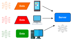
Figure 1. PFL is used to tackle the non-iid data problem.

With the prevalence of the Internet of Things (IoT), massive amounts of data are being collected by heterogeneous edge devices at the end of a network. The deployment of a deep learning neural network is essential to process these data and deliver intelligent services (LeCun et al., 2015). Nevertheless, conventional machine learning approaches usually require edge devices to upload data to a central server for training, which significantly increases the risk of data leakage (Li et al., 2020a). In response to this concern, Federated Learning (FL) emerges as a solution. FL is a distributed machine learning framework that allows edge devices to collaboratively train a model without sharing any private data (McMahan et al., 2017). Orchestrated by a server, devices conduct local machine learning model training and exchange model parameters. Compared to transmitting raw data, FL significantly reduces the risk of data leakage and enhances data privacy. This strength enables FL to offer intelligent services to customers in a wide range of privacy-sensitive applications, such as voice assisting (Leroy et al., 2019), human activity recognition (Yu et al., 2023) and healthcare (Guo et al., 2022).

To effectively deploy FL in real-world IoT systems, it is imperative to consider both data and system heterogeneities among clients. Within an IoT network, clients comprise edge devices that are distributed at various geographical locations. They naturally collect data that are non-independent identical (non-iid). In such a scenario, a single global model struggles to generalize across all local datasets (Kulkarni et al., 2020; Li et al., 2021). To overcome this challenge, the Personalized Federated Learning (PFL) framework is introduced. PFL empowers each client to maintain a unique local model tailored to its local data distribution, effectively addressing the non-iid data challenge, as depicted in Figure 1. Additionally, clients in real-world IoT networks typically consist of physical devices with varying processor, memory, and bandwidth capabilities (Smith et al., 2017; Imteaj et al., 2022). Among these devices, some resource-constrained devices might be incapable of training an entire deep learning model with a too complex structure. To tackle this problem, the technique of federated dropout (i.e. model pruning) is applied. Resource-constrained devices are allowed to train a sub-model, which is a subset of the entire global model, as shown in Figure 2. This approach reduces computation and communication overheads for training and transmitting the sub-model, aiding resource-constrained devices in overcoming computation and communication bottlenecks (Caldas et al., 2018; Horváth et al., 2021).

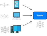
Figure 2. Dropout is used to overcome the computation and communication bottlenecks of resource-constrained devices.

Various PFL frameworks have been developed to tackle the non-iid data challenge, categorized into fine-tuning, personal training and hybrid approaches. Fine-tuning methods (Khodak et al., 2019; Fallah et al., 2020; Arivazhagan et al., 2019; Sattler et al., 2021) fine-tune the global model on the client side post FL completion to acquire personal local models. Personal training methods (Smith et al., 2017; Zhang et al., 2021; Marfoq et al., 2021; Wang et al., 2023; Dinh et al., 2020) empower clients to train personal models rather than a global model, and exchange knowledge through the server. Hybrid methods (Mansour et al., 2020; Deng et al., 2021; Zhang et al., 2023) facilitate clients in simultaneously training local models and the global model.

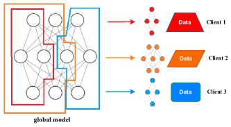
Figure 3. Local dropout usually ends up with sub-models with inconsistent architectures owing to non-iid local data.

Nevertheless, the inherent communication or computation bottleneck of resource-constrained edge devices is often overlooked in these frameworks.

Status Quo and Limitations. To tackle the computation and communication bottlenecks of resource-constrained devices, federated dropout is applied (Caldas et al., 2018; Wen et al., 2022; Horváth et al., 2021; Li et al., 2021; Jiang et al., 2023, 2022), where resource-constrained devices are allowed to train a subset of the global model, i.e. a sub-model. Compared with a full model, the computation and communication overheads for training and transmitting sub-models are reduced, facilitating resource-constrained devices to complete the training task within constraints.

Dropout performs model pruning to create sub-models, including global dropout and local dropout. In global dropout, the server prunes neurons in the global model to create sub-models. For example, in (Caldas et al., 2018; Wen et al., 2022), the server randomly prunes neurons in the global model. In (Horváth et al., 2021), the server prunes the rightmost neurons in the global model. These works fail to meet the personalization requirement, as the server arbitrarily decides the architectures of local sub-models without considering the importance of neurons based on the local data distributions of clients.

On the other hand, local dropout lets clients adaptively prune neurons to obtain the optimal architecture of the local sub-model (Jiang et al., 2023; Li et al., 2021; Jiang et al., 2022). At the beginning, each client trains an initialized model with full architecture to evaluate the importance of each neuron. Then each client locally prunes the unimportant neurons and shares the remaining sub-model with the server hereafter. The importance of a neuron is defined by l1-norm, l2-norm of parameters and gradient l2-norm respectively in (Jiang et al., 2023),(Li et al., 2021),(Jiang et al., 2022). Nevertheless, evaluating neuron importance requires full-model training on the client side, which might be expensive or prohibitive for resource-constrained devices with a critical computation bottleneck.

Furthermore, the adaptive model-pruning behaviors proposed in (Jiang et al., 2023; Li et al., 2021; Jiang et al., 2022) rely immensely on the local data. The non-iid local data distributions often lead to highly unbalanced class distributions across different clients (Puyol-Antón et al., 2021; Padurariu and Breaban, 2019; Wang et al., 2021; Abeysekara et al., 2021). Consequently, the local dropout behavior can be heavily biased (Jiang et al., 2022), and the sub-model architecture among clients may vary drastically, as illustrated in Figure 3. In global communication, when a client absorbs parameters from other clients with inconsistent model architectures, the performance of the local model will be inevitably compromised.

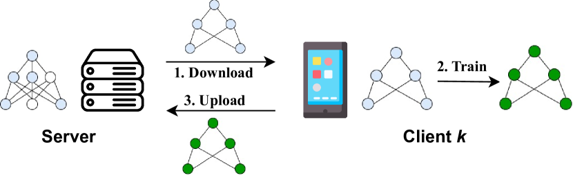
(a) Dropout

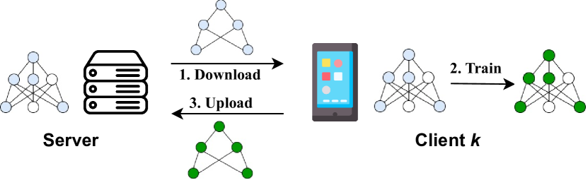
(b) FedSPU

Figure 4. Demonstration of the difference between (a) Dropout and (b) FedSPU. In the former, clients train sub-models with fewer parameters. In the latter, clients train full models with partial parameters frozen.

Overview of the Proposed Solution. To address the limitation of existing works, this paper introduces Federated Learning with Stochastic Parameter Update (FedSPU), a consolidated PFL framework aimed at mitigating the issue of local model personalization loss while considering computation and communication bottlenecks in resource-constrained devices. It is observed that during global communication, a client’s entire local sub-model is replaced by biased parameters of other clients, leading to local model personalization loss. Therefore, if we let a client share only a partial model with others, the adverse effect of other clients’ biased parameters can be alleviated. Inspired by this, FedSPU freezes neurons instead of pruning them, as shown in Figure 4. Frozen neurons do not receive gradients during backpropagation and remain unaltered in subsequent updates. This approach eliminates computation overheads in backward propagation, enhancing computational efficiency. Moreover, FedSPU does not incur extra communication overheads compared with dropout, as only the parameters of the non-frozen neurons and the positions of these neurons are communicated between clients and the server, as depicted in Figure 4. Besides, compared with model parameters, the communication cost for sending the position indices of the non-frozen neurons is much smaller and usually ignorable (Li et al., 2021).

Unlike pruned neurons, frozen neurons persist within a local model’s architecture. During local training, frozen neurons still contribute to the model’s final output, incurring higher computation costs of forward propagation. However, this design choice significantly improves local personalization, as only a portion of a local model is replaced during communication, as shown in Figure 4(b). Despite the increased cost of forward propagation, FedSPU effectively overcomes the computation bottleneck. This is because, in the training process, forward propagation constitutes a significantly smaller portion of the total computation overhead than backpropagation (Li et al., 2020b; He and Sun, 2015). Additionally, to alleviate the additional computation overhead generated by FedSPU and reduce computation and communication costs, we consolidate FedSPU with an early stopping technique (Prechelt, 2002; Niu et al., 2024). At each round, each client locally computes the training and testing errors, and compares them with the errors from the previous round. When the errors show no decrease, this client will cease training and no longer participate in FL. When all clients have halted training, FedSPU will terminate in advance to conserve computation and communication resources.

System Implementation and Evaluation Results. We evaluate the performance of FedSPU on three typical deep learning datasets: EMNIST (Cohen et al., 2017), CIFAR10 (Krizhevsky et al., 2009) and Google Speech (Warden, 2018), with four state-of-the-art dropout methods included for comparison: FjORD (Horváth et al., 2021), Hermes (Li et al., 2021), FedMP (Jiang et al., 2023) and PruneFL (Jiang et al., 2022). Experiment results show that:

• FedSPU consistently outperforms existing dropout methods. It demonstrates an average improvement of 7.57% in final accuracy compared to the best results achieved by dropout.

• FedSPU introduces only minor additional computation overhead. For the entire FL process, the total training time of FedSPU is $1.01\times\sim 1.11\times$ that of the fastest dropout method.

• The early stopping technique remarkably reduces the computation and communication costs in FedSPU. With early stopping, the energy consumption of FedSPU is reduced by $24.8\%\sim 70.4\%$. Compared with existing dropout methods, FedSPU with early stopping reduces the energy consumption by $18\%\sim 70\%$ and maintains an average accuracy improvement of at least 3.35%.

The rest of this paper is structured as follows. Section 2 introduces the background and motivation. Section 3 explains the implementation of FedSPU. Section 4 presents some theoretical analysis of FedSPU. Section 5 shows the experimental results and provides a critical analysis. Section 6 briefly introduces the related work. Section 7 summarizes this article and lists possible future directions.

2. background and motivation

2.1. Personalized Federated Learning

Given a set $\mathbb{C}=\{1,2,...,N\}$ of clients with local datasets $\{D_{1},D_{2},...,D_{N}\}$ and local models $\{w_{1},w_{2},...,w_{N}\}$. The goal of a PFL framework is to determine the optimal set of local models $\{w^{*}_{1},w^{*}_{2},...,w^{*}_{N}\}$ such that:

(1) $$w^{*}_{1},...,w^{*}_{N}\triangleq\mathop{\arg\min}_{w_{1},...,w_{N}}\frac{1}{N}\sum_{k=1}^{N}F_{k}(w_{k})$$

where $w_{k}^{*}$ is the optimal model for client $k$ ($1\leq k\leq N$), and $F_{k}$ is the objective function of client $k$. $F_{k}$ is equivalent to the empirical risk over $k$’s local dataset $D_{k}$. That is:

(2) $$F_{k}(w_{k})=\frac{1}{n_{k}}\sum_{i=1}^{n_{k}}\mathcal{L}((\boldsymbol{x}_{i},y_{i}),w_{k})$$

where $n_{k}$ is the size of dataset $D_{k}$ and $\mathcal{L}$ is the loss function of model $w_{k}$ over the $i-$th sample ($\boldsymbol{x}_{i},y_{i}$).

(a) PruneFL.

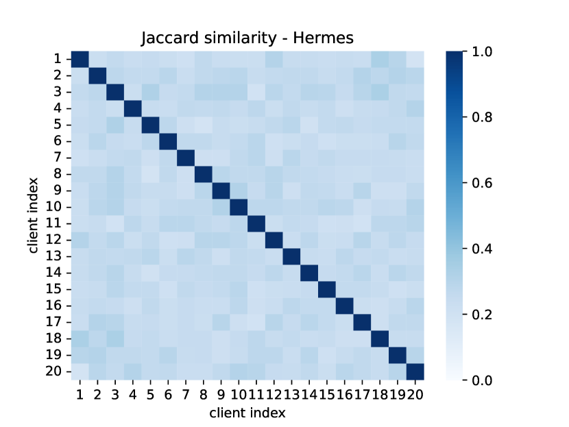
(b) Hermes.

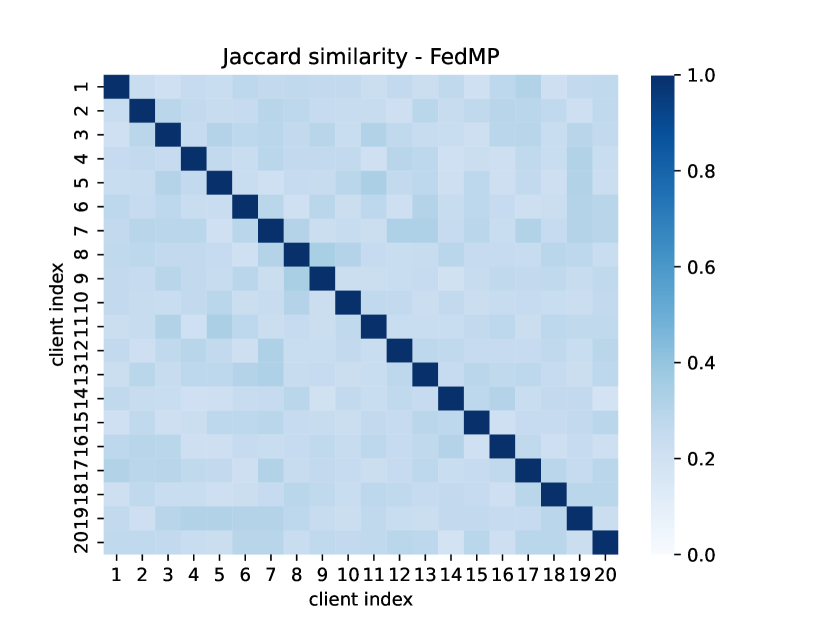
(c) FedMP.

Figure 5. Low Jaccard similarity between local sub-models owing to biased local datasets.

2.2. Divergent Architectures of Biased Local Sub-models

The efficacy of dropout can easily be compromised by the heavy bias of unbalanced local datasets. For illustration, we employed three dropout techniques: PruneFL (Jiang et al., 2022), Hermes (Li et al., 2021) and FedMP (Jiang et al., 2023) on the CIFAR10 (Krizhevsky et al., 2009) dataset with 20 clients. To evaluate the impact of data imbalance, we intentionally distributed data non-uniformly, following a Dirichlet distribution with parameter 0.1 (Acar et al., 2021; Luo et al., 2021). The global model is a convolutional neural network (CNN) with two convolutional layers and three fully-connected layers (Li et al., 2021). After clients have performed model pruning locally, we compute the Jaccard similarity (Jaccard, 1912) between local sub-models following Equation (3):

(3) $$J(w_{j},w_{k})=\frac{|w_{j}\cap w_{k}|}{|w_{j}\cup w_{k}|}$$

where $w_{j}\cap w_{k}$ and $w_{j}\cup w_{k}$ are the joint and union sets of neurons/channels of two local models $w_{j}$ and $w_{k}$ respectively, and $|\cdot|$ is the cardinality of a set.

As depicted in Figure 5, affected by local bias, the Jaccard similarity $J(w_{j},w_{k})$ between any two local sub-models $w_{j}$ and $w_{k}$ ($j\neq k$) is usually low, meaning that their architectures diverge drastically and usually learn contradictory parameter updates in training. Consequently, when a client incorporates others’ biased parameters, the performance of the local model will be inevitably compromised.

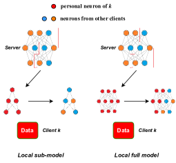
Figure 6. Comparison between replacing all parameters of a local sub-model and replacing a portion of the parameters for a local full model during global communication.

2.3. Full Local Model Preserves Personalization

FedSPU freezes neurons instead of pruning them to preserve the integrity of the local model architecture, thereby preserving the personalization of local models. For clarity, Figure 6 shows a comparison between a local sub-model and a local full model. As shown in the left-hand side of Figure 6, in global communication, when receiving other clients’ biased parameters from the server, the entire local sub-model is replaced, resulting in a loss of personalization. Conversely, as illustrated in the right-hand side of Figure 6, for a local full model, only partial parameters are replaced, while the remainder remains personalized. This limits the adverse effect of biased parameters from other clients, enabling the local model to maintain performance on the local dataset.

To validate this hypothesis, we assess the performance of FedSPU, FjORD, FedMP, PruneFL and Hermers on the CIFAR10 dataset over 500 training rounds involving 100 clients. The experiment is conducted with three degrees of data imbalance, with the number of samples per class following three Dirichlet distributions with parameters 0.1, 0.5 and 1.0. As depicted in Figure 7, FedSPU obtains the highest accuracy in all cases, exhibiting the strength of local full models in maintaining personalization.

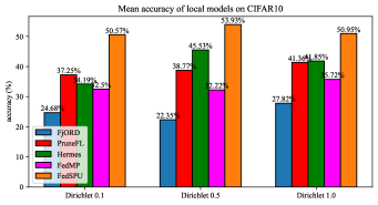
Figure 7. FedSPU (full local models) achieves better performance than dropout methods (local sub-models).

3. Methodology

3.1. Overview of FedSPU

An overview of FedSPU is presented in Figure 8. As shown in Figure 8(a), at round $t$, the server randomly selects a set of participating clients $\mathbb{C}_{t}$ and executes steps ①$\sim$④.

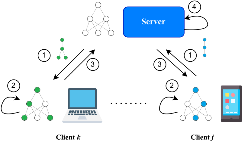
(a) Overview of FedSPU.

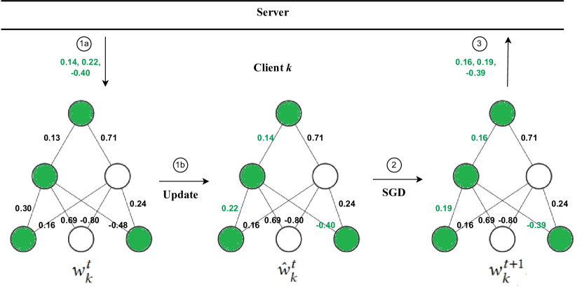
(b) The local training procedure of client $k$ in FedSPU.

Figure 8. Demonstration of the FedSPU framework.

①. For every participating client $k$, the server selects a set of active neurons from the global model, and sends the neurons’ parameters $A_{k}(w^{t})$ to $k$. Specifically, in each layer, random $p_{k}$ of the neurons are selected, where $p_{k}\in(0,1]$ is the ratio of active neurons. The value of $p_{k}$ depends on the system characteristic of the client $k$, with more powerful $k$’s device having larger $p_{k}$. The active neurons are selected randomly to ensure uniform parameter updates. Locally, client $k$ updates the local model $w_{k}^{t}$ with the received $A_{k}(w^{t})$ to obtain an intermediate model $\hat{w}_{k}^{t}$ as shown in Figure 8(b).

②. Client $k$ updates model $\hat{w}_{k}^{t}$ using stochastic gradient descent (SGD) to get a new model $w_{k}^{t+1}$ following Equation (4):

(4) $$w_{k}^{t+1}=\hat{w}_{k}^{t}-\eta\nabla\bar{F}_{k}(\hat{w}_{k}^{t})$$

where $\eta$ is the learning rate and $\nabla\bar{F}_{k}(\hat{w}_{k}^{t})$ is the gradient of $F_{k}$ with respect to only the active parameters. That is, for all elements {$\hat{w}_{k,1}^{t},...,\hat{w}_{k,m}^{t}$} in $\hat{w}_{k}^{t}$, we have:

(5) $$\nabla\bar{F}_{k}(\hat{w}^{t}_{k,i})=\begin{cases}\nabla F_{k}(\hat{w}^{t}_{k,i}),&\hat{w}^{t}_{k,i}\in A_{k}(w^{t})\\ 0,&\text{otherwise.}\end{cases},1\leq i\leq m$$

In this step, only the active parameters are updated as shown in Figure 8(b).

③. Client $k$ uploads the updated active parameters $A_{k}(w_{k}^{t+1})$ to the server.

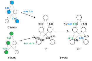
Figure 9. Sample illustration demonstrating how the server aggregates parameters and updates the global model in FedSPU.

④. The server aggregates all updated parameters and updates the global model. In this step, FedSPU applies a standard aggregation scheme commonly used in existing dropout methods, where only the active parameters get aggregated and updated (Caldas et al., 2018; Horváth et al., 2021; Li et al., 2021). Figure 9 shows a simple example of how the aggregation scheme works, where ”WA” stands for weighted average.

Combining all these steps, a comprehensive framework of FedSPU is presented in Algorithm 1.

Algorithm 1 FedSPU

1:maximum global iteration $T$, clients $\mathbb{C}=\{1,...,N\}$, initial global model $w^{0}$.

2:Server broadcasts $w_{0}$ to all clients.

3:For round $t=1,2,...,T$:

4:Server executes:

5:    randomly sample a subset of clients $\mathbb{C}_{t}\subset\mathbb{C}$.

6:    $\forall k\in\mathbb{C}_{t}$:

7:       randomly sample $A_{k}(w^{t})$ based on $p_{k}$.

8:       send $A_{k}(w^{t})$ to $k$.

9:Each client $k\in\mathbb{C}_{t}$ in parallel does:

10:    merge $A_{k}(w^{t})$ into $w_{k}^{t}$ to get $\hat{w}^{t}_{k}$. $\triangleright$ see Fig. 8(b)

11:    local training: $w_{k}^{t+1}=\hat{w}_{k}^{t}-\eta\nabla\bar{F}_{k}(\hat{w}_{k}^{t})$. $\triangleright$ see Eq. (4)

12:    send $A_{k}(w_{k}^{t+1})$ to the server. $\triangleright$ see Fig. 8(b)

13:Server executes:

14:    $\forall k\in\mathbb{C}_{t}$:

15:       receive $A_{k}(w_{k}^{t+1})$ from $k$.

16:    Aggregate all $A_{k}(w_{k}^{t+1})$ to get $w^{t+1}$. $\triangleright$ see Fig. 9

17:return $w_{1},w_{2},...,w_{N}$.

3.2. Enhancing FedSPU with Early Stopping Strategy

Since FedSPU slightly increases the computation overhead, it requires more computation resources (e.g., energy (Imteaj et al., 2022), time (He and Sun, 2015)) for training. This may pose a challenge for resource-constrained devices. To address this concern, it is expected to reduce the training time of FedSPU without sacrificing accuracy (Niu et al., 2024). Motivated by this, we enhance FedSPU with the Early Stopping (ES) technique (Prechelt, 2002) to prevent clients from unnecessary training to avoid the substantial consumption of computation and communication resources.

At round $t$, after training, each client $k\in\mathbb{C}_{t}$ computes $\mathcal{L}_{t}$ following Equation (6):

(6) $$\mathcal{L}_{t}=\lambda\mathcal{L}_{train}+(1-\lambda)\mathcal{L}_{test}$$

where $\mathcal{L}_{train}$ is the training error of current round $t$, $\mathcal{L}_{test}$ is the testing error of $w_{k}^{t}$ on $k$’s validation set. $\lambda\in(0,1)$ is the train-test split factor of the local dataset $D_{k}$. When the loss $\mathcal{L}_{t}$ is non-decreasing, i.e. $\mathcal{L}_{t}>\mathcal{L}_{t-1}$, client $k$ will stop training and no longer participate in FL due to resource concerns. If all clients have stopped training before the maximum global iteration $T$, FedSPU will terminate prematurely. The enhanced FedSPU framework is detailed in Algorithm 2.

Algorithm 2 FedSPU with Early Stopping

1:maximum global iteration $T$, clients $\mathbb{C}=\{1,...,N\}$, initial global model $w^{0}$.

2:Server broadcasts $w_{0}$ to all clients.

3:For round $t=1,2,...,T$:

4:Server executes:

5:    randomly sample a subset of clients $\mathbb{C}_{t}\subset\mathbb{C}$.

6:    $\forall k\in\mathbb{C}_{t}$:

7:       randomly sample $A_{k}(w^{t})$ based on $p_{k}$.

8:       send $A_{k}(w^{t})$ to $k$.

9:Each client $k\in\mathbb{C}_{t}$ in parallel does:

10:    merge $A_{k}(w^{t})$ into $w_{k}^{t}$ to get $\hat{w}^{t}_{k}$. $\triangleright$ see Fig. 8(b)

11:    local training: $w_{k}^{t+1}=\hat{w}_{k}^{t}-\eta\nabla\bar{F}_{k}(\hat{w}_{k}^{t})$. $\triangleright$ see Eq. (4)

12:    compute $\mathcal{L}_{t}$. $\triangleright$ see Eq. (6)

13:    If $\mathcal{L}_{t}>\mathcal{L}_{t-1}$:

14:       status $\leftarrow$ stopped

15:    Else:

16:       status $\leftarrow$ on

17:    send $A_{k}(w_{k}^{t+1})$ and status to the server.

18:Server executes:

19:    $\forall k\in\mathbb{C}_{t}$:

20:       receive $A_{k}(w_{k}^{t+1})$, status from $k$.

21:       If status == stopped:

22:         remove $k$ from $\mathbb{C}$.

23:    Aggregate all $A_{k}(w_{k}^{t+1})$ to get $w^{t+1}$. $\triangleright$ see Fig. 9

24:    If $\mathbb{C}==\varnothing$:

25:       TERMINATE.

26:return $w_{1},w_{2},...,w_{N}$.

4. Theoretical analysis

This section analyzes the convergence of each local model to support the validity of FedSPU. First of all, we make the following assumptions:

Assumption 1.Every local objective function $F_{k}$ is $L-$smooth:

$$\forall w_{1},w_{2},F_{k}(w_{2})-F_{k}(w_{1})\leq\langle\nabla F_{k}(w_{1}),w_{2}-w_{1}\rangle+\frac{L}{2}\|w_{2}-w_{1}\|^{2}.$$

Assumption 2. The divergence between local gradients with and without incorporating the parameter received from the server is bounded:

$$\exists\ Q>0,\forall\ k,t,\ \frac{\mathbb{E}(\|\nabla F_{k}(w_{k}^{t})\|^{2})}{\mathbb{E}(\|\nabla F_{k}(\hat{w}_{k}^{t})\|^{2})}\leq Q.$$

Assumption 3. The divergence between the local parameters with and without incorporating the parameter received from the server is bounded:

$$\exists\ \sigma>0,\forall\ k,t,\ \mathbb{E}(\|\hat{w}_{k}^{t}-w_{k}^{t}\|^{2})\leq\sigma^{2}.$$

With respect to the gradient $\nabla\bar{F}_{k}$, we derive the following lemmas:

Lemma 1. $\forall\ w_{k},\ \mathbb{E}(\|\bar{F}_{k}(w_{k})\|^{2})=p_{k}^{2}\ \|F_{k}(w_{k})\|^{2}$.

Proof. As defined in FedSPU, a parameter $w_{k,i}$ in $w_{k}$ is active only when the two neurons it connects are both active, and the probability of the two neurons being both active is $p_{k}^{2}$. Therefore:

(7) $$\begin{split}&\mathbb{E}(\|\nabla\bar{F}_{k}(w_{k})\|^{2})\\ &=\mathbb{E}(\sum_{i}^{n}\nabla\bar{F}_{k}(w_{k,i})^{2})\\ &=\sum_{i}^{n}\mathbb{E}(\nabla\bar{F}_{k}(w_{k,i})^{2})\\ &=p_{k}^{2}(\nabla F_{k}(w_{k,1})^{2}+\nabla F_{k}(w_{k,2})^{2}+...+\nabla F_{k}(w_{k,m})^{2})\\ &=p_{k}^{2}\ \|\nabla F_{k}(w_{k})\|^{2}.\\ \end{split}$$

Lemma 2. $\forall w_{k},\langle\nabla F_{k}(w_{k}),\nabla\bar{F}_{k}(w_{k})\rangle=\|\nabla\bar{F}_{k}(w_{k})\|^{2}$.

Proof.

(8) $$\begin{split}&\hskip 14.22636pt\langle\nabla F_{k}(w_{k}),\nabla\bar{F}_{k}(w_{k})\rangle\\ &=\sum_{i}F_{k}(w_{k,i})\ \bar{F}_{k}(w_{k,i})\\ &=\sum_{i,i\not\in A(w_{k})}F_{k}(w_{k,i})\ \bar{F}_{k}(w_{k,i})+\sum_{i,i\in A(w_{k})}F_{k}(w_{k,i})\ \bar{F}_{k}(w_{k,i})\\ &=0+\sum_{i,i\in A(w_{k})}F_{k}(w_{k,i})\ \bar{F}_{k}(w_{k,i})\hskip 42.67912pt\text{See Eq. (\ref{eq:barfk})}\\ &=\sum_{i,i\in A(w_{k})}F_{k}(w_{k,i})^{2}\\ &=\|\nabla\bar{F}_{k}(w_{k})\|^{2}.\\ \end{split}$$

Based on Assumptions 1-3 and Lemmas 1 and 2, the following theorem holds:

Theorem 1. When the learning rate $\eta$ satisfies $\eta<\frac{1+\sqrt{1-\frac{QL}{p_{k}^{2}}}}{L}$, every local model $w_{k}$ will at least reach a $\epsilon$-critical point $w_{k}^{\epsilon}$ (i.e. $\|\nabla F_{k}(w_{k}^{\epsilon})\|\leq\epsilon$) in $O(\frac{w_{k}^{0}-w_{k}^{\epsilon}}{\epsilon\eta})$ rounds, with $\epsilon=\sqrt{\frac{(L+1)Q\sigma^{2}}{(2\eta-L\eta^{2})p_{k}^{2}+Q}}$.

Proof. As $F_{k}$ is $L-smooth$, we have:

(9) $$\begin{split}&F_{k}({w}_{k}^{t+1})-F_{k}(\hat{w}_{k}^{t})\\ &\leq\langle\nabla F_{k}(\hat{w}_{k}),w_{k}^{t+1}-\hat{w}_{k}^{t}\rangle+\frac{L}{2}\|w_{k}^{t+1}-\hat{w}_{k}^{t}\|^{2}\\ &=-\eta\|\nabla\bar{F}_{k}(\hat{w}_{k}^{t})\|^{2}+\frac{L\eta^{2}}{2}\|\nabla\bar{F}_{k}(\hat{w}_{k}^{t})\|^{2}\\ &=(-\eta+\frac{L\eta^{2}}{2})\|\nabla\bar{F}_{k}(\hat{w}_{k}^{t})\|^{2}.\\ \end{split}$$

and:

(10) $$\begin{split}&F_{k}(\hat{w}_{k}^{t})-F_{k}({w}_{k}^{t})\\ &\leq\langle\nabla F_{k}(w_{k}),\hat{w}_{k}^{t}-w_{k}^{t}\rangle+\frac{L}{2}\|\hat{w}_{k}^{t}-w_{k}^{t}\|^{2}\\ &\leq\frac{1}{2}\|\nabla F_{k}(w_{k}^{t})\|^{2}+\frac{1}{2}\|\hat{w}_{k}^{t}-w_{k}^{t}\|^{2}+\frac{L}{2}\|\hat{w}_{k}^{t}-w_{k}^{t}\|^{2}.\\ \end{split}$$

By adding (9) and (10), we obtain:

(11) $$\begin{split}&F_{k}(w_{k}^{t+1})-F_{k}({w}_{k}^{t})\\ &\leq(-\eta+\frac{L\eta^{2}}{2})\|\nabla\bar{F}_{k}(\hat{w}_{k}^{t})\|^{2}+\frac{1}{2}\|\nabla F_{k}(w_{k}^{t})\|^{2}+\frac{L+1}{2}\|\hat{w}_{k}^{t}-w_{k}^{t}\|^{2}.\\ \end{split}$$

By taking the expectation of both sides, we obtain:

(12) $$\begin{split}&\mathbb{E}(F_{k}(w_{k}^{t+1})-F_{k}({w}_{k}^{t}))\\ &\leq(-\eta+\frac{L\eta^{2}}{2})\ \mathbb{E}(\|\nabla\bar{F}_{k}(\hat{w}_{k}^{t})\|^{2})\\ &\hskip 14.22636pt+\frac{1}{2}\mathbb{E}(\|\nabla F_{k}(w_{k}^{t})\|^{2})+\frac{L+1}{2}\mathbb{E}(\|\hat{w}_{k}^{t}-w_{k}^{t}\|^{2}).\\ &\leq(-\eta+\frac{L\eta^{2}}{2})\ \mathbb{E}(\|\nabla\bar{F}_{k}(\hat{w}_{k}^{t})\|^{2})\\ &\hskip 14.22636pt\ +\frac{1}{2}\mathbb{E}(\|\nabla F_{k}(w_{k}^{t})\|^{2})+\frac{L+1}{2}\sigma^{2}.\\ \end{split}$$

Since $\frac{1}{2}\mathbb{E}(\|\nabla F_{k}(w_{k}^{t})\|^{2})+\frac{L+1}{2}\sigma^{2}$ is always positive, in order for $F_{k}$ to decrease, we need $(-\eta+\frac{L\eta^{2}}{2})\ \mathbb{E}(\|\nabla\bar{F}_{k}(\hat{w}_{k}^{t})\|^{2})$ to be less than 0, i.e. $\eta<\frac{2}{L}$.

Furthermore, based on Lemma 1 and Assumption 2, we have $\mathbb{E}(\|\nabla\bar{F}_{k}(\hat{w}_{k}^{t})\|^{2})=p_{k}^{2}\ \mathbb{E}(\|\nabla F_{k}(\hat{w}_{k}^{t})\|^{2})\geq\frac{1}{Q}\ p_{k}^{2}\ \mathbb{E}(\|\nabla F_{k}(w_{k}^{t})\|^{2})$. Therefore:

(13) $$\begin{split}&\mathbb{E}(F_{k}(w_{k}^{t+1})-F_{k}({w}_{k}^{t}))\\ &\leq((-\eta+\frac{L\eta^{2}}{2})\frac{p_{k}^{2}}{Q}+\frac{1}{2})\ \mathbb{E}(\|\nabla F_{k}(w_{k}^{t})\|^{2})+\frac{L+1}{2}\sigma^{2}.\\ \end{split}$$

When $(-\eta+\frac{L\eta^{2}}{2})\frac{p_{k}}{Q}^{2}+\frac{1}{2}<0$, i.e. $\eta<\frac{1+\sqrt{1-\frac{QL}{p_{k}^{2}}}}{L}$, the expectation of $F_{k}$ keeps decreasing until $\mathbb{E}(\|\nabla F_{k}(w_{k}^{t})\|^{2})<\frac{(L+1)Q\sigma^{2}}{(2\eta-L\eta^{2})p_{k}^{2}+Q}$. This means that, given $\eta<\frac{1+\sqrt{1-\frac{QL}{p_{k}^{2}}}}{L}$, client $k$’s local model $w_{k}$ will at least reach a $\epsilon$-critical point (i.e. $\|\nabla F_{k}(w_{k})\|\leq\epsilon$), with $\epsilon=\sqrt{\frac{(L+1)Q\sigma^{2}}{(2\eta-L\eta^{2})p_{k}^{2}+Q}}$.

Let $w_{k}^{0}$ be client $k$’s initial model, then the time complexity for client $k$ to reach $w_{k}^{\epsilon}$ is $O(\frac{w_{k}^{0}-w_{k}^{\epsilon}}{\epsilon\eta})$. It is worth mentioning that $\eta<\frac{1+\sqrt{1-\frac{QL}{p_{k}^{2}}}}{L}$ also satisfies $\eta<\frac{2}{L}$ as $1+\sqrt{1-\frac{QL}{p_{k}^{2}}}<2$.

According to Theorem 1, in FedSPU, each client’s local objective function will converge to a relatively low value, given that the learning rate is small enough. This means that every client’s personal model will eventually acquire favorable performance on the local dataset even if the objective function is not necessarily convex.

5. evaluation

This section presents the experimental details elucidating the efficacy of FedSPU in enhancing PFL performance, particularly in scenarios with computation and communication bottlenecks.

5.1. Experiment Setup

Datasets and models. We evaluate FedSPU on three real-world datasets that are very commonly used in the state-of-the-art, including:

• Extended MNIST (EMNIST) contains 814,255 images of human-written digits/characters from 62 categories (numbers 0-9 and 52 upper/lower-case English letters). Each sample is a black-and-white-based image with $28\times 28$ pixels (Cohen et al., 2017).

• CIFAR10 contains 50,000 images of real-world objects across 10 categories. Each sample is an RGB-based colorful image with $32\times 32$ pixels (Krizhevsky et al., 2009).

• Google Speech is an audio dataset containing 101,012 audio commands from more than 2,000 speakers. Each sample is a human-spoken word belonging to one of the 35 categories (Warden, 2018).

For EMNIST and Google Speech, a convolutional neural network (CNN) with two convolutional layers and one fully-connected layer is used, following the setting of (Horváth et al., 2021). For CIFAR10, a CNN with two convolutional layers and three fully-connected layers is used, following the setting of (Li et al., 2021).

To simulate unbalanced local data distributions, we allocate data to clients unevenly same as the settings of (Acar et al., 2021; Luo et al., 2021), following a Dirichlet distribution with parameter $\alpha$. We tune the value of $\alpha$ with 0.1, 0.5 and 1.0 to create three different distributions of local datasets. We split each client’s dataset into a training set and a testing set with the split factor $\lambda=0.7$.

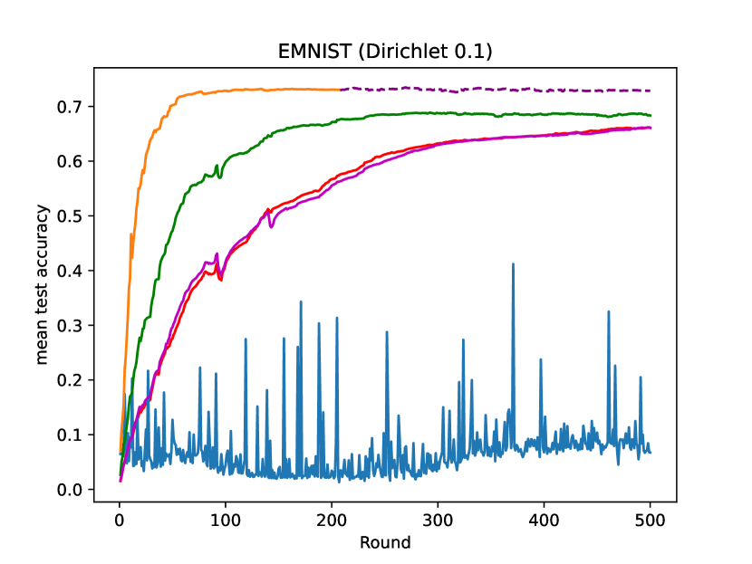
(a) $\alpha=0.1$

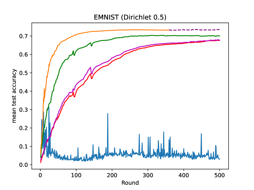
(b) $\alpha=0.5$

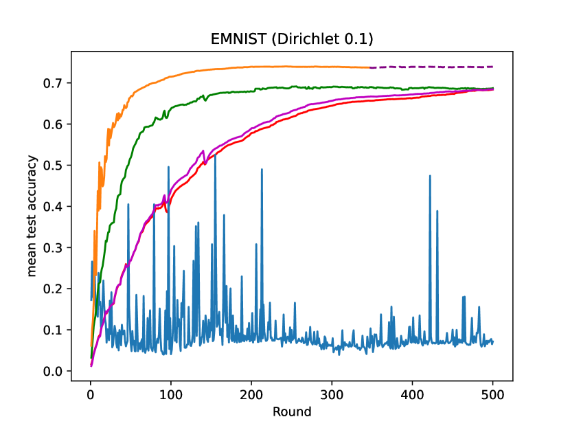
(c) $\alpha=1.0$

Figure 10. Comparison of accuracy on EMNIST.

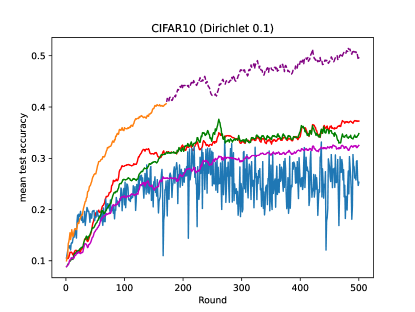
(a) $\alpha=0.1$

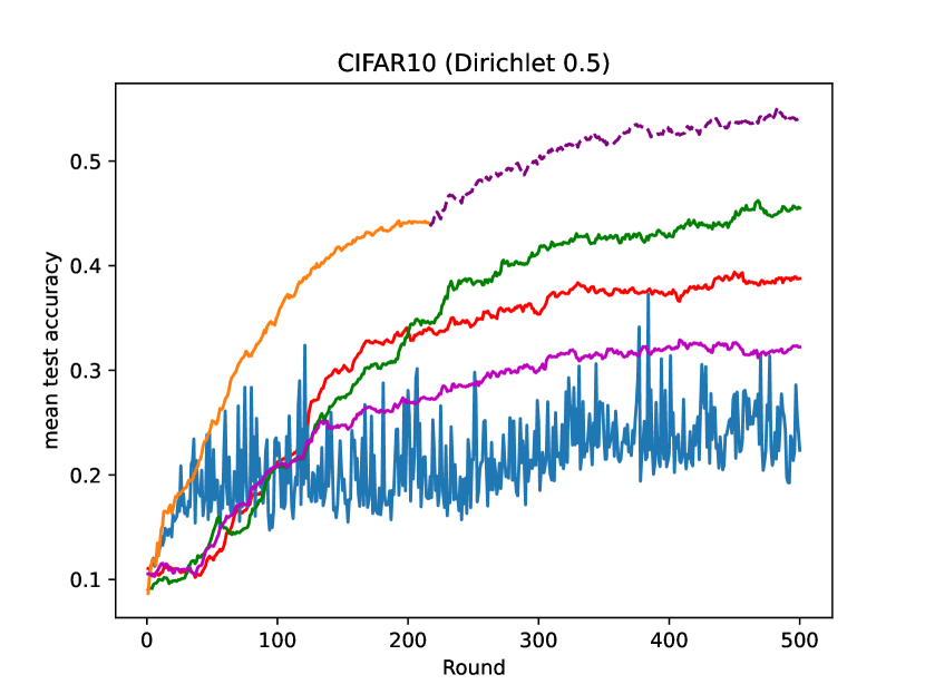
(b) $\alpha=0.5$

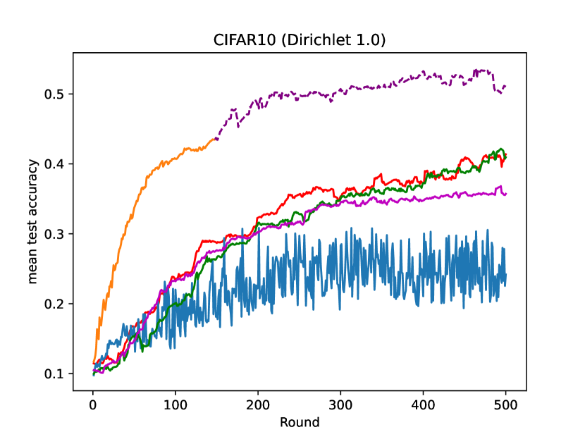
(c) $\alpha=1.0$

Figure 11. Comparison of accuracy on CIFAR10.

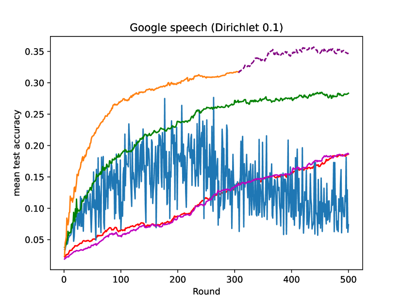
(a) $\alpha=0.1$

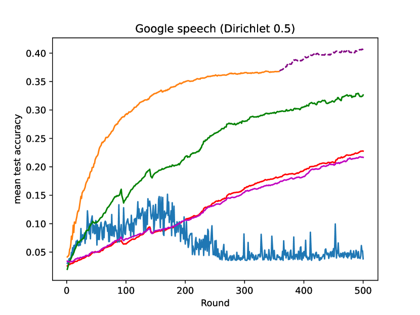
(b) $\alpha=0.5$

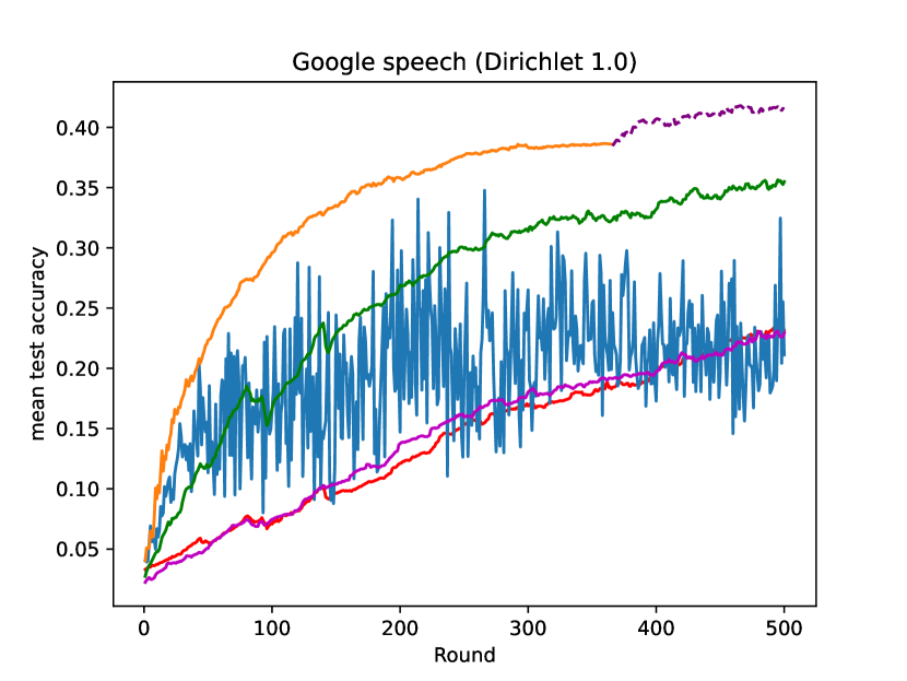
(c) $\alpha=1.0$

Figure 12. Comparison of accuracy on Google Speech.

Dataset/Distribution	PruneFL	FjORD	Hermes	FedMP	FedSPU	FedSPU+ES
EMNIST ($\alpha=0.1$)	66.10%	8.37%	68.66%	66.08%	72.89%	73.04%
EMNIST ($\alpha=0.5$)	67.57%	3.72%	70.03%	67.77%	73.53%	73.18%
EMNIST ($\alpha=1.0$)	68.37%	7.31%	68.60%	68.43%	73.86%	73.73%
CIFAR10 ($\alpha=0.1$)	37.25%	24.68%	34.19%	32.50%	50.57%	40.46%
CIFAR10 ($\alpha=0.5$)	38.77%	22.35%	45.53%	32.22%	53.93%	44.06%
CIFAR10 ($\alpha=1.0$)	33.95%	27.82%	41.85%	35.72%	50.95%	43.47%
Google Speech ($\alpha=0.1$)	18.62%	7.39%	27.97%	18.66%	35.14%	31.75%
Google Speech ($\alpha=0.5$)	22.76%	5.21%	32.64%	21.66%	40.52%	36.76%
Google Speech ($\alpha=1.0$)	23.13%	21.12%	35.49%	22.92%	41.64%	38.60%
Average	41.83%	14.21%	47.21%	40.66%	54.78%	50.56%

Table 1. Final test accuracy.

Parameter settings and system implementation. For all datasets, the maximum global iteration is set to $T=500$, with a total of $M=100$ clients. The number of selected clients per round is set to 10, and each selected client has five local training epochs (Horváth et al., 2021). Specifically, for FedSPU with ES, if the number of non-stopped clients is less than 10, then all non-stopped clients will be selected. The learning rate is set to 2e-4, 5e-4 and 0.1 respectively for EMNIST, Google Speech and CIFAR10. The batch size is set to 16 for EMNIST and Google Speech, and 128 for CIFAR10. The experiment is implemented with Pytorch 2.0.0 and the Flower framework (Beutel et al., 2022). The server runs on a desktop computer and clients run on NVIDIA Jetson Nano Developer Kits with one 128-core Maxwell GPU and 4GB 64-bit memory (nan, [n. d.]). For the emulation of system heterogeneity and resource constraints, we divide the clients into 5 uniform clusters following (Horváth et al., 2021). Clients of the same cluster share the same value of $p_{k}$. The values of $p_{k}$ for the five clusters are 0.2, 0.4, 0.6, 0.8 and 1.0 respectively.

Baselines We compare FedSPU with four typical federated dropout methods, all baselines follow the same parameter settings as FedSPU:

• FjORD (Horváth et al., 2021): is a global dropout method. The server prunes neurons in a fixed right-to-left order. In each layer of the global model, the $1-p_{k}$ of the rightmost neurons are pruned, and the remaining $p_{k}$ are sent to client $k$ as the local sub-model.

• FedMP (Jiang et al., 2023) is a local dropout method. The server first broadcasts the global model to all clients. Then each client $k$ locally prunes neurons to create a personal sub-model. In each layer, $1-p_{k}$ of the neurons with the least importance scores are pruned. The importance of a neuron is defined as the l1-norm of the parameters.

• Hermes (Li et al., 2021) is a local dropout method. Similar to FedMP, each client $k$ locally prunes the $1-p_{k}$ least important neurons in each layer after receiving the global model from the server. The importance of a neuron is defined as the l2-norm of the parameters.

• PruneFL (Jiang et al., 2022) is a local dropout method. Similarly, each client $k$ locally prunes the $1-p_{k}$ least important neurons in each layer. The importance of a neuron is defined as the l2-norm of the neuron’s gradient.

The typical Random Dropout (Caldas et al., 2018) method which lets all clients collaboratively train a single global model, is not included for comparison in this PFL setting. For local dropout, finding the unimportant neurons requires full-model training, which might be prohibitive for resource-constrained devices. For a fair comparison, we neglect the computation bottlenecks and let each client pre-train the local model for one iteration to enable clients to identify the unimportant neurons.

5.2. Experiment results

Dataset/Distribution	PruneFL	FjORD	Hermes	FedMP	FedSPU	FedSPU+ES
EMNIST ($\alpha=0.1$)	8.11	7.85	8.57	7.30	7.82	3.23
EMNIST ($\alpha=0.5$)	8.09	7.89	8.55	7.29	7.83	5.42
EMNIST ($\alpha=1.0$)	8.09	7.89	8.56	7.28	7.78	5.38
CIFAR10 ($\alpha=0.1$)	24.65	25.16	24.81	25.55	25.01	8.58
CIFAR10 ($\alpha=0.5$)	24.70	25.08	25.18	25.56	25.07	10.78
CIFAR10 ($\alpha=1.0$)	24.73	24.86	25.21	25.48	25.08	7.34
Google Speech ($\alpha=0.1$)	8.28	7.81	8.08	8.16	8.71	5.33
Google Speech ($\alpha=0.5$)	8.31	7.88	8.11	8.16	8.73	6.24
Google Speech ($\alpha=1.0$)	8.28	7.80	8.11	8.16	8.70	6.34

Table 2. Comparison of total training time (hours) for $T=500$ rounds, where total training time represents the duration of the entire FL process excluding global communication time.

FedSPU results in significant improvement in accuracy relative to dropout while maintaining convergence. As shown by Figures 10, 11, 12, the learning curve of FedSPU lies above all baselines’ curves in most cases. This means that FedSPU can achieve higher accuracy than dropout given the same rounds of training. With the improved learning speed, FedSPU obtains higher final accuracy than dropout as Table 1 shows. On average, FedSPU improves the final test accuracy by $7.57\%$ compared with the best results of dropout (Hermes). Moreover, the smooth learning curves in Figures 10, 11, 12 also demonstrate the ability of FedSPU to maintain the convergence of each local model. These results prove the usefulness of local full models in preserving personalization.

Computation overhead. To assess computation overhead, we compare the wall-clock training time of FedSPU with the baselines, which is a common criterion to measure the computation cost of training a deep-learning model (Bonawitz et al., 2019; He and Sun, 2015; Li et al., 2022; Zhang et al., 2023). For each method, the total training time is computed as the total time of the entire FL process minus the total time for global communication. As shown by Table 2, the additional computation overhead caused by FedSPU is minor, as the training time of FedSPU is not significantly higher than other dropout methods. In some cases, FedSPU even spends less time on training than dropout, for example, for EMNIST with $\alpha=0.1$, FedSPU consumes the second least training time among all methods (7.82 hours), only slightly higher than FedMP (7.30 hours). Among all cases, the training time of FedSPU is $1.01\times\sim 1.11\times$ that of the fastest baseline.

Dataset/Distribution	PruneFL	FjORD	Hermes	FedMP	FedSPU	FedSPU+ES
EMNIST ($\alpha=0.1$)	11.63GB	11.72GB	11.70GB	11.72GB	11.75GB	4.82GB
EMNIST ($\alpha=0.5$)	11.79GB	11.72GB	11.64GB	11.56GB	11.71GB	8.80GB
EMNIST ($\alpha=1.0$)	11.65GB	11.71GB	11.80GB	11.72GB	11.69GB	8.07GB
CIFAR10 ($\alpha=0.1$)	18.32GB	18.23GB	18.00GB	18.44GB	18.04GB	6.14GB
CIFAR10 ($\alpha=0.5$)	18.24GB	18.24GB	18.18GB	18.38GB	17.92GB	7.71GB
CIFAR10 ($\alpha=1.0$)	18.05GB	18.05GB	18.42GB	18.49GB	18.17GB	5.27GB
Google Speech ($\alpha=0.1$)	4.39GB	4.38GB	4.35GB	4.34GB	4.37GB	2.68GB
Google Speech ($\alpha=0.5$)	4.38GB	4.37GB	4.38GB	4.35GB	4.38GB	3.12GB
Google Speech ($\alpha=1.0$)	4.38GB	4.34GB	4.36GB	4.41GB	4.35GB	3.17GB

Table 3. Comparison of the total size of transmitted parameters.

Additionally, Table 2 presents an interesting phenomenon. That is, even though FedSPU increases the cost of forward propagation in training, the training time of FedSPU is not necessarily higher than dropout. We attribute this phenomenon to the fact that the computation cost primarily arises from backpropagation, involving the computation of parameter gradients (Li et al., 2020b). The complexity of gradient computation, however, is contingent on the depth of the neural network, i.e. number of layers. For instance, in PyTorch, the computational overhead primarily results from backward propagation, tracing the gradient graph throughout the entire neural network, with the complexity of the graph being intricately tied to the network’s depth (gra, [n. d.]). While dropout scales the width of the neural network, it has a limited impact on training time reduction, as training is susceptible to various real-world factors like CPU/GPU temperature, voltage and memory. This explains the instances where dropout even consumes more training time than FedSPU. Inspired by this observation, our future work aims to devise more effective methods (e.g. pruning layers) to mitigate training time.

Dataset/	Rounds		Final accuracy			Expected cost
Distribution	FedSPU	FedSPU+ES	FedSPU	FedSPU+ES	Change	FedSPU	FedSPU+ES	Saving
EMNIST ($\alpha=0.1$)	500	207	72.89%	73.04%	+0.15%	$1\times$	$0.41\times$	59%
EMNIST ($\alpha=0.5$)	500	374	73.53%	73.18%	-0.35%	$1\times$	$0.75\times$	25%
EMNIST ($\alpha=1.0$)	500	346	73.86%	73.73%	-0.13%	$1\times$	$0.69\times$	31%
CIFAR10 ($\alpha=0.1$)	500	171	50.57%	40.46%	-10.11%	$1\times$	$0.34\times$	66%
CIFAR10 ($\alpha=0.5$)	500	216	53.93%	44.06%	-9.87%	$1\times$	$0.43\times$	57%
CIFAR10 ($\alpha=1.0$)	500	147	50.95%	43.47%	-7.48%	$1\times$	$0.29\times$	71%
Google Speech ($\alpha=0.1$)	500	306	35.14%	31.75%	-3.39%	$1\times$	$0.61\times$	39%
Google Speech ($\alpha=0.5$)	500	358	40.52%	36.76%	-3.76%	$1\times$	$0.71\times$	29%
Google Speech ($\alpha=1.0$)	500	365	41.64%	38.60%	-3.04%	$1\times$	$0.73\times$	27%

Table 4. Comparison of final accuracy and estimated computation and communication cost (combined) between FedSPU and FedSPU with early stopping.

Communication overhead. Compared with dropout, FedSPU does not incur extra communication overhead for every single client, as only the active parameters will be communicated between a client and the server as shown in Figure 4. Moreover, since both FedSPU and dropout employ a random client selection strategy, the expectation of the overall communication cost of FedSPU and dropout will be the same. To verify this, we measure the total size of the transmitted message of FedSPU and the baselines. As shown in Table 3, there is very little difference between the size of the transmitted parameters in FedSPU and the baselines.

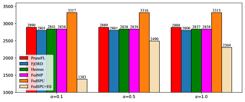
(a) EMNIST

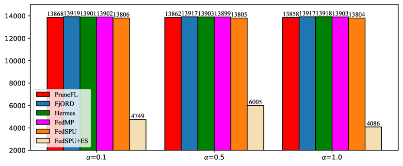
(b) CIFAR10

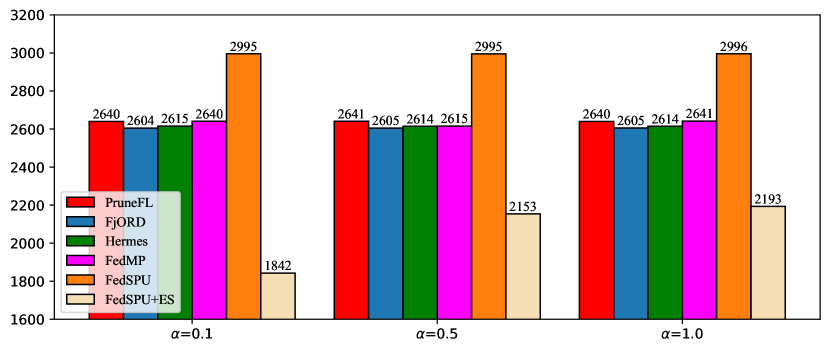
(c) Google Speech

Figure 13. Comparison of overall energy consumption (Unit: kJ).

The early stopping strategy effectively reduces the computation and communication costs in FedSPU. With early stopping (ES), the number of training rounds of FedSPU is reduced by $25\%\sim 71\%$ as shown in Table 4. Correspondingly, the total computation and communication overheads are expected to be reduced by $25\%\sim 71\%$ as well as shown in Tables 2 and 3. To verify this, we examine the overall energy consumption of all clients by measuring their power usage on the Jetson Nano Developer Kits with a power monitor (mon, [n. d.]), including the computation energy for local training and the communication energy for transmitting parameters. As shown in Figure 13, the total energy consumption in FedSPU+ES is trimmed down by $24.8\%\sim 70.4\%$ compared with FedSPU sole, which is very close to our estimation.

To assess the impact of ES on accuracy, Table 4 presents a comparison between FedSPU and FedSPU+ES. For EMNIST and Google Speech, ES effectively reduces the computation/communication cost by $25\%\sim 59\%$ in FedSPU with a marginal accuracy sacrifice of no more than 3.76%. For CIFAR10, the ES strategy becomes more aggressive, reducing the cost by $57\%\sim 71\%$ with $7.48\%\sim 10.11\%$ of accuracy loss. Despite this, the final accuracy of FedSPU+ES is still higher than that of dropout in most cases as shown in Table 1. The only exception is CIFAR10 with $\alpha=0.5$, where the final accuracy of FedSPU+ES ($44.06\%$) is slightly lower than Hermes (45.53%). Based on the results of Figure 13 and Table 1, FedSPU with ES requires $18\%\sim 70\%$ less energy consumption to acquire at least 3.35% improvement in average accuracy compared to dropout. This positions it as a viable choice for IoT systems with resource constraints. Additionally, we do not consider integrating ES with other dropout methods as they are unable to preserve accuracy compared with FedSPU.

6. Related work

6.1. Personalized Federated Learning

Personalized federated learning has been developed to address the non-iid data problem in federated learning. To the best of our knowledge, existing personalized federated learning methods can be divided into three categories. 1) Fine-tuning: All clients at first train a global model collaboratively, followed by individual fine-tuning to adapt to local datasets. In (Arivazhagan et al., 2019), each client fine-tunes some layers of the global model to adapt to the local dataset. (Fallah et al., 2020) proposes to find an initial global model that generalizes well to all clients through model-agnostic-meta-learning formulation, afterwards, all clients fine-tune the model locally through just a few gradient steps. (Khodak et al., 2019) proposes to improve the global model’s generalization with dynamic learning rate adaption based on the squared difference between local gradients, which significantly reduces the workload of local fine-tuning. (Sattler et al., 2021) fine-tunes the global model based on clusters, and clients from the same cluster share the same local model. 2) Personal Training: Clients train personal models at the beginning. (Dinh et al., 2020) adds a regularization term to each local objective function that keeps local models from diverging too far from the global model to improve the global model’s generalization. (Marfoq et al., 2021) assumes each local data distribution is a mixture of several unknown distributions, and optimizes each local model with the expectation-maximization algorithm. (Smith et al., 2017) speeds up the convergence of each local model by modeling local training as a primal-dual optimization problem. (Wang et al., 2023) lets each client maintain a personal head while training to improve the global model’s generalization by aggregating local heads on the server side. (Zhang et al., 2021) proposes to train local models through first-order optimization, where the local objective function becomes the error subtraction between clients. 3) Hybrid: Clients merge local and global models to foster mutual learning and maintain personalization. In (Deng et al., 2021; Mansour et al., 2020; Zhang et al., 2023), each client simultaneously trains the global model and its local model. The ultimate model for each client is a combination of the global and the local model.

Even though these works potently address the non-iid data problem in FL, they neglect the computation or communication bottleneck of resource-constrained IoT devices.

6.2. Dropout in Federated Learning

In centralized machine learning, dropout is used as a regularization method to prevent a neural network from over-fitting (Srivastava et al., 2014). Nowadays, as federated learning becomes popular in the IoT industry, dropout has also been applied to address the computation and communication bottlenecks of resource-constrained IoT devices. In dropout, clients are allowed to train and transmit a subset of the global model to reduce the computation and communication overheads. To extract a subset from the global model, i.e. a sub-model, Random Dropout (Caldas et al., 2018; Wen et al., 2022) randomly prune neurons in the global model. FjORD (Horváth et al., 2021) continually prunes the right-most neurons in a neural network. FedMP (Jiang et al., 2023), Hermes (Li et al., 2021) and PruneFL (Jiang et al., 2022) let clients adaptively prune the unimportant neurons, and the importance of a neuron is the l1-norm, l2-norm of parameters, and l2-norm of gradient respectively.

Random Dropout and FjORD represent global dropout methods and do not meet the personalization requirement, as the server arbitrarily prunes neurons without considering clients’ non-iid data. On the other hand, local dropout methods such as FedMP, Hermes, and PruneFL may be hindered by the bias of unbalanced local datasets.

Compared with existing works, FedSPU comprehensively meets the personalization requirement and addresses the computation and communication bottlenecks of resource-constrained devices, meanwhile overcoming data imbalance.

7. conclusion

We propose FedSPU, a novel personalized federated learning approach with stochastic parameter update. FedSPU preserves the global model architecture on each edge device, randomly freezing portions of the local model based on device capacity, training the remaining segments with local data, and subsequently updating the model based solely on the trained segments. This methodology ensures that a segment of the local model remains personalized, thereby mitigating the adverse effects of biased parameters from other clients. We also introduced an early stopping scheme to accelerate the training, which further reduces computation and communication costs while maintaining high accuracy. In the future, we plan to explore the similarities of local clients in a privacy-preserving way, leveraging techniques such as learning vector quantization (Qin and Suganthan, 2005) and graph matching (Gong et al., 2016) to guide the model freezing process and enhance local model training. Furthermore, we intend to enhance the generalization capabilities of the global model.

References

- (1)
- mon ([n. d.]) Amazon [n. d.]. 240V Plug Power Meter Electricity Usage Monitor,PIOGHAX Energy Watt Voltage Amps Meter with Backlit Digital LCD, Overload Protection and 7 Display Modes for Energy Saving. Amazon. https://www.amazon.com.au/Electricity-Monitor-PIOGHAX-Overload-Protection/dp/B09SFSB66M
- gra ([n. d.]) Pytorch [n. d.]. How Computational Graphs are Executed in PyTorch. Pytorch. https://pytorch.org/blog/how-computational-graphs-are-executed-in-pytorch/
- nan ([n. d.]) NVIDIA [n. d.]. Jetson Nano Developer Kit. NVIDIA. https://developer.nvidia.com/embedded/jetson-nano-developer-kit
- Abeysekara et al. (2021) Prabath Abeysekara, Hai Dong, and A. K. Qin. 2021. Data-Driven Trust Prediction in Mobile Edge Computing-Based IoT Systems. IEEE Transactions on Services Computing (2021).
- Acar et al. (2021) Durmus Alp Emre Acar, Yue Zhao, Ramon Matas, Matthew Mattina, Paul Whatmough, and Venkatesh Saligrama. 2021. Federated Learning Based on Dynamic Regularization. In International Conference on Learning Representations.
- Arivazhagan et al. (2019) Manoj Ghuhan Arivazhagan, Vinay Aggarwal, Aaditya Kumar Singh, and Sunav Choudhary. 2019. Federated Learning with Personalization Layers. arXiv:1912.00818 [cs.LG]
- Beutel et al. (2022) Daniel J. Beutel, Taner Topal, Akhil Mathur, Xinchi Qiu, Javier Fernandez-Marques, Yan Gao, Lorenzo Sani, Kwing Hei Li, Titouan Parcollet, Pedro Porto Buarque de Gusmão, and Nicholas D. Lane. 2022. Flower: A Friendly Federated Learning Research Framework. arXiv:2007.14390 [cs.LG]
- Bonawitz et al. (2019) Keith Bonawitz, Hubert Eichner, Wolfgang Grieskamp, Dzmitry Huba, Alex Ingerman, Vladimir Ivanov, Chloé Kiddon, Jakub Konečný, Stefano Mazzocchi, Brendan McMahan, Timon Van Overveldt, David Petrou, Daniel Ramage, and Jason Roselander. 2019. Towards Federated Learning at Scale: System Design. In Proceedings of Machine Learning and Systems, A. Talwalkar, V. Smith, and M. Zaharia (Eds.), Vol. 1. 374–388.
- Caldas et al. (2018) Sebastian Caldas, Jakub Konečny, H. Brendan McMahan, and Ameet Talwalkar. 2018. Expanding the Reach of Federated Learning by Reducing Client Resource Requirements. In NeurIPS Workshop on Federated Learning for Data Privacy and Confidentiality.
- Cohen et al. (2017) Gregory Cohen, Saeed Afshar, Jonathan Tapson, and André van Schaik. 2017. EMNIST: an extension of MNIST to handwritten letters. arXiv preprint arXiv:1702.05373 (2017).
- Deng et al. (2021) Yuyang Deng, Mohammad Mahdi Kamani, and Mehrdad Mahdavi. 2021. Adaptive Personalized Federated Learning.
- Dinh et al. (2020) Canh T. Dinh, Nguyen H. Tran, and Tuan Dung Nguyen. 2020. Personalized Federated Learning with Moreau Envelopes. In Proceedings of the 34th International Conference on Neural Information Processing Systems (Vancouver, BC, Canada) (NIPS’20). Curran Associates Inc., Red Hook, NY, USA, 12 pages.
- Fallah et al. (2020) Alireza Fallah, Aryan Mokhtari, and Asuman Ozdaglar. 2020. Personalized Federated Learning: A Meta-Learning Approach. arXiv:2002.07948 [cs.LG]
- Gong et al. (2016) Maoguo Gong, Yue Wu, Qing Cai, Wenping Ma, A. K. Qin, Zhenkun Wang, and Licheng Jiao. 2016. Discrete particle swarm optimization for high-order graph matching. Information Sciences 328 (2016), 158–171.
- Guo et al. (2022) Kehua Guo, Tianyu Chen, Sheng Ren, Nan Li, Min Hu, and Jian Kang. 2022. Federated Learning Empowered Real-Time Medical Data Processing Method for Smart Healthcare. IEEE/ACM Transactions on Computational Biology and Bioinformatics (2022), 1–12.
- He and Sun (2015) Kaiming He and Jian Sun. 2015. Convolutional neural networks at constrained time cost. In Proceedings of the IEEE conference on computer vision and pattern recognition. 5353–5360.
- Horváth et al. (2021) Samuel Horváth, Stefanos Laskaridis, Mario Almeida, Ilias Leontiadis, Stylianos Venieris, and Nicholas Lane. 2021. FjORD: Fair and Accurate Federated Learning under heterogeneous targets with Ordered Dropout. In Advances in Neural Information Processing Systems, M. Ranzato, A. Beygelzimer, Y. Dauphin, P.S. Liang, and J. Wortman Vaughan (Eds.), Vol. 34. Curran Associates, Inc., 12876–12889.
- Imteaj et al. (2022) Ahmed Imteaj, Urmish Thakker, Shiqiang Wang, Jian Li, and M. Hadi Amini. 2022. A Survey on Federated Learning for Resource-Constrained IoT Devices. IEEE Internet of Things Journal 9, 1 (2022), 1–24.
- Jaccard (1912) Paul. Jaccard. 1912. The distribution of the flora in the alpine zone.1. New Phytologist 11 (1912), 37–50. Issue 2.
- Jiang et al. (2022) Yuang Jiang, Shiqiang Wang, Victor Valls, Bong Jun Ko, Wei-Han Lee, Kin K Leung, and Leandros Tassiulas. 2022. Model pruning enables efficient federated learning on edge devices. IEEE Transactions on Neural Networks and Learning Systems (2022).
- Jiang et al. (2023) Zhida Jiang, Yang Xu, Hongli Xu, Zhiyuan Wang, Jianchun Liu, Qian Chen, and Chunming Qiao. 2023. Computation and Communication Efficient Federated Learning With Adaptive Model Pruning. IEEE Transactions on Mobile Computing (2023), 1–18.
- Khodak et al. (2019) Mikhail Khodak, Maria-Florina F Balcan, and Ameet S Talwalkar. 2019. Adaptive gradient-based meta-learning methods. Advances in Neural Information Processing Systems 32 (2019).
- Krizhevsky et al. (2009) Alex Krizhevsky et al. 2009. Learning multiple layers of features from tiny images. (2009).
- Kulkarni et al. (2020) Viraj Kulkarni, Milind Kulkarni, and Aniruddha Pant. 2020. Survey of Personalization Techniques for Federated Learning. arXiv:2003.08673 [cs.LG]
- LeCun et al. (2015) Yann LeCun, Yoshua Bengio, and Geoffrey Hinton. 2015. Deep learning. nature 521, 7553 (2015), 436–444.
- Leroy et al. (2019) David Leroy, Alice Coucke, Thibaut Lavril, Thibault Gisselbrecht, and Joseph Dureau. 2019. Federated Learning for Keyword Spotting. In ICASSP 2019 - 2019 IEEE International Conference on Acoustics, Speech and Signal Processing (ICASSP). 6341–6345.
- Li et al. (2021) Ang Li, Jingwei Sun, Pengcheng Li, Yu Pu, Hai Li, and Yiran Chen. 2021. Hermes: An Efficient Federated Learning Framework for Heterogeneous Mobile Clients. In Proceedings of ACM MobiCom. Association for Computing Machinery, New York, NY, USA, 420–437.
- Li et al. (2022) Chenning Li, Xiao Zeng, Mi Zhang, and Zhichao Cao. 2022. PyramidFL: A Fine-Grained Client Selection Framework for Efficient Federated Learning. In Proceedings of ACM MobiCom. Association for Computing Machinery, New York, NY, USA, 158–171.
- Li et al. (2020b) Shen Li, Yanli Zhao, Rohan Varma, Omkar Salpekar, Pieter Noordhuis, Teng Li, Adam Paszke, Jeff Smith, Brian Vaughan, Pritam Damania, and Soumith Chintala. 2020b. PyTorch Distributed: Experiences on Accelerating Data Parallel Training. Proc. VLDB Endow. 13 (2020), 3005–3018.
- Li et al. (2020a) Tian Li, Anit Kumar Sahu, Ameet Talwalkar, and Virginia Smith. 2020a. Federated Learning: Challenges, Methods, and Future Directions. IEEE Signal Processing Maganize 37, 3 (2020), 50–60.
- Luo et al. (2021) Mi Luo, Fei Chen, Dapeng Hu, Yifan Zhang, Jian Liang, and Jiashi Feng. 2021. No Fear of Heterogeneity: Classifier Calibration for Federated Learning with Non-IID Data. In Advances in Neural Information Processing Systems, A. Beygelzimer, Y. Dauphin, P. Liang, and J. Wortman Vaughan (Eds.).
- Mansour et al. (2020) Yishay Mansour, Mehryar Mohri, Jae Ro, and Ananda Theertha Suresh. 2020. Three Approaches for Personalization with Applications to Federated Learning. arXiv:2002.10619 [cs.LG]
- Marfoq et al. (2021) Othmane Marfoq, Giovanni Neglia, Aurélien Bellet, Laetitia Kameni, and Richard Vidal. 2021. Federated Multi-Task Learning under a Mixture of Distributions. In Advances in Neural Information Processing Systems, A. Beygelzimer, Y. Dauphin, P. Liang, and J. Wortman Vaughan (Eds.).
- McMahan et al. (2017) Brendan McMahan, Eider Moore, Daniel Ramage, Seth Hampson, and Blaise Aguera y Arcas. 2017. Communication-Efficient Learning of Deep Networks from Decentralized Data. In Artificial Intelligence and Statistics (AISTAS). 1273–1282.
- Niu et al. (2024) Ziru Niu, Hai Dong, A. Kai Qin, and Tao Gu. 2024. FLrce: Resource-Efficient Federated Learning with Early-Stopping Strategy. arXiv:2310.09789 [cs.LG]
- Padurariu and Breaban (2019) Cristian Padurariu and Mihaela Elena Breaban. 2019. Dealing with Data Imbalance in Text Classification. Procedia Computer Science 159 (2019), 736–745. Knowledge-Based and Intelligent Information & Engineering Systems: Proceedings of the 23rd International Conference KES2019.
- Prechelt (2002) Lutz Prechelt. 2002. Early Stopping - But When? In Neural Networks: Tricks of the trade. Springer, 55–69.
- Puyol-Antón et al. (2021) Esther Puyol-Antón, Bram Ruijsink, Stefan K. Piechnik, Stefan Neubauer, Steffen E. Petersen, Reza Razavi, and Andrew P. King. 2021. Fairness in Cardiac MR Image Analysis: An Investigation of Bias Due to Data Imbalance in Deep Learning Based Segmentation. In Medical Image Computing and Computer Assisted Intervention – MICCAI 2021, Marleen de Bruijne, Philippe C. Cattin, Stéphane Cotin, Nicolas Padoy, Stefanie Speidel, Yefeng Zheng, and Caroline Essert (Eds.). Springer International Publishing, Cham, 413–423.
- Qin and Suganthan (2005) A. K. Qin and P. N. Suganthan. 2005. Initialization insensitive LVQ algorithm based on cost-function adaptation. Pattern Recognition 38, 5 (2005), 773–776.
- Sattler et al. (2021) Felix Sattler, Klaus-Robert Müller, and Wojciech Samek. 2021. Clustered Federated Learning: Model-Agnostic Distributed Multitask Optimization Under Privacy Constraints. IEEE Transactions on Neural Networks and Learning Systems 32, 8 (2021), 3710–3722.
- Smith et al. (2017) Virginia Smith, Chao-Kai Chiang, Maziar Sanjabi, and Ameet S Talwalkar. 2017. Federated multi-task learning. Advances in neural information processing systems 30 (2017).
- Srivastava et al. (2014) Nitish Srivastava, Geoffrey Hinton, Alex Krizhevsky, Ilya Sutskever, and Ruslan Salakhutdinov. 2014. Dropout: A Simple Way to Prevent Neural Networks from Overfitting. Journal of Machine Learning Research 15, 56 (2014), 1929–1958.
- Wang et al. (2021) Le Wang, Meng Han, Xiaojuan Li, Ni Zhang, and Haodong Cheng. 2021. Review of Classification Methods on Unbalanced Data Sets. IEEE Access 9 (2021), 64606–64628.
- Wang et al. (2023) Yansong Wang, Hui Xu, Waqar Ali, Miaobo Li, Xiangmin Zhou, and Jie Shao. 2023. FedFTHA: A Fine-Tuning and Head Aggregation Method in Federated Learning. IEEE Internet of Things Journal 10, 14 (2023), 12749–12762.
- Warden (2018) Pete Warden. 2018. Speech Commands: A Dataset for Limited-Vocabulary Speech Recognition. arXiv preprint arXiv:1804.03209 (2018).
- Wen et al. (2022) Dingzhu Wen, Ki-Jun Jeon, and Kaibin Huang. 2022. Federated Dropout – A Simple Approach for Enabling Federated Learning on Resource Constrained Devices. arXiv:2109.15258 [cs.LG]
- Yu et al. (2023) Hongzheng Yu, Zekai Chen, Xiao Zhang, Xu Chen, Fuzhen Zhuang, Hui Xiong, and Xiuzhen Cheng. 2023. FedHAR: Semi-Supervised Online Learning for Personalized Federated Human Activity Recognition. IEEE Transactions on Mobile Computing 22, 6 (2023), 3318–3332.
- Zhang et al. (2023) Jianqing Zhang, Yang Hua, Hao Wang, Tao Song, Zhengui Xue, Ruhui Ma, and Haibing Guan. 2023. FedALA: Adaptive Local Aggregation for Personalized Federated Learning. Proceedings of the AAAI Conference on Artificial Intelligence 37 (June 2023), 11237–11244.
- Zhang et al. (2021) Michael Zhang, Karan Sapra, Sanja Fidler, Serena Yeung, and Jose M. Alvarez. 2021. Personalized Federated Learning with First Order Model Optimization. In International Conference on Learning Representations.