Clustering theorem in 1D long-range interacting systems at arbitrary temperatures

Abstract

This paper delves into a fundamental aspect of quantum statistical mechanics—the absence of thermal phase transitions in one-dimensional (1D) systems. Originating from Ising’s analysis of the 1D spin chain, this concept has been pivotal in understanding 1D quantum phases, especially those with finite-range interactions as extended by Araki. In this work, we focus on quantum long-range interactions and successfully derive a clustering theorem applicable to a wide range of interaction decays at arbitrary temperatures. This theorem applies to any interaction forms that decay faster than $r^{-2}$ and does not rely on translation invariance or infinite system size assumptions. Also, we rigorously established that the temperature dependence of the correlation length is given by $e^{{\rm const.}\beta}$, which is the same as the classical cases. Our findings indicate the absence of phase transitions in 1D systems with super-polynomially decaying interactions, thereby expanding upon previous theoretical research. To overcome significant technical challenges originating from the divergence of the imaginary-time Lieb-Robinson bound, we utilize the quantum belief propagation to refine the cluster expansion method. This approach allowed us to address divergence issues effectively and contributed to a deeper understanding of low-temperature behaviors in 1D quantum systems.

I Introduction

One of the most fundamental aspects of quantum statistical mechanics is the absence of thermal phase transition in one-dimensional (1D) systems. This concept has historical roots tracing back to the seminal work of Ising [1], who solved the one-dimensional spin chain problem, thereby illuminating the lack of phase transition in 1D. Building upon this, Araki [2] extended these insights into the quantum domain by investigating general quantum spin systems with finite-range interactions, particularly in the thermodynamic limit. In quantum equilibrium states, non-critical phases are typically characterized by a finite correlation length for bi-partite correlations within quantum Gibbs states. Furthermore, the analyticity of the partition function [3] and the uniqueness of the Kubo-Martin-Schwinger (KMS) state [4, 5, 6] are also recognized as alternative hallmarks of non-criticality in these systems.

In contrast to one-dimensional (1D) systems, thermal phase transitions are more prevalent in higher-dimensional systems and have been a subject of extensive study in the history of statistical mechanics [7, 8]. In these higher-dimensional settings, the absence of phase transitions is typically only guaranteed at higher temperatures. Interestingly, even within the confines of one dimension, it has been known that long-range interactions, characterized by a slow decay in interaction strength, can lead to thermal phase transitions. This poses a significant question regarding the occurrence of thermal phase transitions under interactions of varying ranges, a topic that has been actively researched for many decades. The nature of these interactions is often modeled by the polynomial decay with distance $r$, expressed as $r^{-\alpha}$. Here, the critical value of $\alpha$ plays a crucial role: In classical theory, if $\alpha\leq 2$, it indicates the presence of a thermal phase transition [9, 10, 11, 12], whereas $\alpha>2$ suggests its absence [13]. Further insights can be found in the footnote .

A pivotal question in the study of quantum long-range interacting chains is the determination of the regime of $\alpha$ that ensures non-criticality at arbitrary temperatures. While initial studies, such as those by Araki [15] and Kishimoto [16], have established the uniqueness of the KMS state in 1D systems with long-range interactions for $\alpha>2$, it has been still challenging to characterize the 1D quantum phases beyond these foundational works. Remarkably, it has been over half a century since the generalization of the methodologies used in Araki’s seminal work [2]. In [2], the analysis of the 1D Ising model was conducted using an intricate operator algebra technique. This advanced mathematical approach enabled the exploration of phase transitions within a specific scope, notably in systems where interactions were of finite range and exhibited translational invariance. However, the complexity of these methods presented substantial challenges in generalizing the analyses to broader system classes, particularly in contexts where these constraints were not met. As a result, the pursuit of understanding phase transitions in more generalized settings remained a formidable task, underscoring the need for novel approaches in this field of research.

In recent developments, the paper by Pérez-García et al. [17] has shed light on the challenges in generalizing the understanding of quantum long-range interacting systems. A significant hurdle identified is the divergence of the imaginary-time Lieb-Robinson bound, which describes the quasi-locality of systems after undergoing imaginary-time evolution. This divergence, as generally proven in [18], implies that an imaginary-time-evolved local operator becomes entirely non-local across the whole system after a threshold time. However, in one-dimensional systems with finite-range interactions, this quasi-locality is preserved for any imaginary time. In these cases, the length scale of the quasi-locality increases exponentially with imaginary time, as detailed in [19, Lemma 1] for example. Extending beyond finite-range interactions, Pérez-García et al. [17] demonstrated that the convergence of the imaginary Lieb-Robinson bound is attainable as long as the interaction decays super-exponentially with distance. For interactions that decay exponentially or slower, the imaginary Lieb-Robinson bound remains convergent only below a specific threshold time. This insight indicates that any attempt to generalize beyond exponentially decaying interactions requires the development of alternative mathematical techniques to effectively handle one-dimensional quantum Gibbs states.

In our current work, we address a portion of this open problem and derive a clustering theorem applicable to any form of interaction decay at arbitrary temperatures. The merits of our results are summarized as follows:

1. The theorem is applicable to all forms of interaction, provided the decay rate is faster than $r^{-2}$ [see the assumption (4)].

2. Our result is established unconditionally, meaning we do not assume translation invariance or infinite system size. Moreover, for slower decay of interactions than subexponential form, the obtained decay rate for the bi-correlation is qualitatively optimal in the sense that it shows qualitatively the same behavior as the interaction decay (see Theorem 1).

3. We determine the explicit form of the correlation length $\xi_{\beta}$ as a function of the inverse temperature $\beta$ . In detail, we identified $\xi_{\beta}=e^{{\rm const.}\times\beta}$. This is qualitatively optimal since the correlation length in the classical Ising model has an exponential dependence on the inverse temperature.

These strengths enable the broad application of our findings, extending and generalizing the scope of previous works based on Araki’s foundational studies [2]. Examples include clustering theorems for mutual information [20] and conditional mutual information [21], studies on rapid thermalization [22], and the equivalence of statistical mechanical ensembles [23, 24, 25], efficient simulation of the quantum Gibbs state [26], among others. However, our results are not without limitations:

1. In the case of exponentially decaying interactions, the decay rate of the bi-partite correlation function is subexponential, following $e^{-\Omega(\sqrt{R})}$ (where $R$ denotes distance), rather than an exponential form.

2. Our findings do not extend to the analyticity of the partition function. For finite systems, analyzing the positions of complex zeroes in the partition function is essential [27]. Currently, our techniques appear limited in analyzing quantum Gibbs states at complex temperatures.

Despite these limitations, our research significantly enhances the understanding of the structure of 1D quantum Gibbs states at low temperatures. Notably, our results suggest the absence of phase transitions in any one-dimensional system with super-polynomially decaying interactions, a significant extension from previous results [17] limited to super-exponentially decaying interactions.

Finally, we highlight our principal technical contributions in this work. To address the challenge of the divergence of the imaginary Lieb-Robinson bound, we have integrated the quantum belief propagation technique [28, 29] with the established Lieb-Robinson bound [30, 31]. This combination is pivotal in the recent advancements in the field of low-temperature quantum many-body physics [32, 33, 34, 35]. We show the basic techniques in Sec. III. Our approach utilizes the quantum belief propagation method to refine the cluster expansion technique (see Sec. IV). Typically, the expansion encounters divergence beyond a certain temperature threshold, even in one-dimensional systems [36, 37, 38, 39, 40, 41]. To circumvent this issue at arbitrary temperatures, we draw upon strategies from classical cases, where divergence can be more readily avoided through the use of a standard transfer-matrix method (see Sec. IV.1). In our exploration, we identify several challenges in extending these classical methods to quantum scenarios. Our paper proposes solutions to these challenges (see Sec. V), primarily through careful treatment of the cluster expansion. This approach not only addresses the immediate issue of divergence but also contributes to a broader understanding of quantum systems and their behaviors at low temperatures.

II Setup

Consider a quantum system comprising $n$ spins, or qudits, arrayed along a one-dimensional (1D) chain. We represent the total set of spins by $\Lambda$. For an arbitrary subset $X$ within $\Lambda$, denoted as $X\subseteq\Lambda$, the cardinality of $X$—the number of sites it contains—is indicated by $|X|$. With a total of $n$ spins in the system, it follows that $|\Lambda|=n$. For a sequence of subsets $X_{1},X_{2},\ldots,X_{q}$, we adopt the notation of $X_{1:q}=X_{1}\cup X_{2}\cup\cdots\cup X_{q}$. For any two subsets $X,Y$ in $\Lambda$, with $X,Y\subseteq\Lambda$, we define the distance between these sets, $d_{X,Y}$, as the minimum path length on the graph connecting $X$ and $Y$. It is important to note that if $X$ and $Y$ have an intersection, such that $X\cap Y\neq\emptyset$, the distance between $X$ and $Y$ is considered to be zero: $d_{X,Y}=0$. Furthermore, when $X$ comprises a single element, specifically when $X=\{i\}$, we simplify the notation for distance from $d_{\{i\},Y}$ to $d_{i,Y}$ for ease of reference. We denote the complementary set of $X$ by $X^{\rm c}$, defined as $X^{\rm c}:=\Lambda\setminus X$, and the surface subset of $X$ by $\partial X$, i.e., $\partial X:=\{i\in X\,|\,d_{i,X^{\rm c}}=1\}$.

We consider a general $k$-local Hamiltonian $H$ described by:

$$H=\sum_{Z:|Z|\leq k}h_{Z}\quad(h_{Z}\succeq 0),$$ (1)

where $h_{Z}$ is an positive semidefinite operator supported on the subset $Z\subset\Lambda$ with $|Z|\leq k$. Note that any $k$-local Hamiltonian can be given by the above form by shifting the energy origin. For an arbitrary subset $L$, we denote the subset Hamiltonian supported on $L$ by $H_{L}$:

$$H_{X}=\sum_{Z:Z\subseteq L}h_{Z}.$$ (2)

We here characterize the interaction decays as follows:

$$J_{i,i^{\prime}}:=\sum_{Z:Z\ni\{i,i^{\prime}\}}\left\|h_{Z}\right\|\leq g\bar{J}(d_{i,i^{\prime}}),$$ (3)

where $\bar{J}(x)$ is an arbitrary function that monotonically decays with $x$ and $\bar{J}(0)=1$. We assume that $\bar{J}(x)$ decays faster than $1/x^{2}$ in the following sense:

$$\sum_{x=\ell}^{\infty}x^{z}\bar{J}(x)\leq\gamma\ell^{z+1}\bar{J}(\ell),\quad\gamma=\mathcal{O}(1)\quad\textrm{for}\quad z\leq 1,\quad\ell\in\mathbb{N}^{+}.$$ (4)

We note that the one-site energy is upper-bounded by $g$:

$$\sum_{Z:Z\ni i}\left\|h_{Z}\right\|\leq g\bar{J}(0)=g.$$ (5)

We consider the quantum Gibbs state $\rho_{\beta}$ with a fixed inverse temperature $\beta$, defined as:

$$\rho_{\beta}:=\frac{e^{\beta H}}{Z_{\beta}},\quad Z_{\beta}={\rm tr}\left(e^{\beta H}\right),$$ (6)

where the minus sign is included in the Hamiltonian without loss of generality. Additionally, we introduce a function of the variables $x_{1},x_{2},\ldots,x_{s}$, denoted as $\Theta(x_{1},x_{2},\ldots,x_{s})$, which is defined by

$$\Theta(x_{1},x_{2},\ldots,x_{s})=\sum_{\sigma_{1},\sigma_{2},\ldots,\sigma_{s}=0,1}c_{\sigma_{1},\sigma_{2},\ldots,\sigma_{s}}x_{1}^{\sigma_{1}}x_{2}^{\sigma_{2}}\cdots x_{s}^{\sigma_{s}}\quad(0<c_{\sigma_{1},\sigma_{2},\ldots,\sigma_{s}}<\infty).$$ (7)

The coefficients, $c_{\sigma_{1},\sigma_{2},\ldots,\sigma_{s}}$, are dependent only on the fundamental parameters $g$, $k$ and $\gamma$.

For an arbitrary operator $O$, we define the time evolution of $O$ by another operator $O^{\prime}$ (e.g., a subset Hamiltonian $H_{L}$) as

$$O(O^{\prime},t):=e^{iO^{\prime}t}Oe^{-iO^{\prime}t}.$$ (8)

For simplicity, we usually denote $O(H,t)$ by $O(t)$.

Following Ref. [14, Supplementary Lemma 2], we prove the statement as follows:

Lemma 1.

Let us define the interaction operator $V_{L,L^{\prime}}(\Lambda_{0})$ between two subsystems $L\subset\Lambda$ and $L^{\prime}\subset\Lambda$ as follows:

$$V_{L,L^{\prime}}(\Lambda_{0}):=\sum_{\begin{subarray}{c}Z:Z\subset\Lambda_{0}\\ Z\cap L\neq\emptyset,Z\cap L^{\prime}\neq\emptyset\end{subarray}}h_{Z}.$$ (9)

Here, $V_{L,L^{\prime}}(\Lambda_{0})$ characterizes the block-block interactions between $L$ and $L^{\prime}$ acting on the region $\Lambda_{0}$. Then, the norm of $V_{L,L^{\prime}}(\Lambda_{0})$ is bounded from above by

$$\|V_{L,L^{\prime}}(\Lambda_{0})\|\leq g\gamma^{2}r^{2}\bar{J}(r),$$ (10)

where the function $\bar{J}(r)$ is defined in Eq. (3).

Proof of Lemma 1. In our proof, we aim to calculate the upper bound of the term $\overline{V}_{L,L^{\prime}}$, defined as:

$$\overline{V}_{L,L^{\prime}}:=\sum_{\begin{subarray}{c}Z:Z\cap L\neq\emptyset,\\ Z\cap L^{\prime}\neq\emptyset\end{subarray}}\|h_{Z}\|,$$ (11)

which serves as an upper bound for $\|V_{L,L^{\prime}}(\Lambda_{0})\|$ for any subset $\Lambda_{0}\subset\Lambda$. Assuming that the subsystem $L^{\prime}$ is located to the right of $L$, we define $L=\{i_{0}-n_{L}+1,i_{0}-n_{L}+2,\ldots,i_{0}\}$ $L^{\prime}=\{i_{0}+r,i_{0}+r+1,\ldots,i_{0}+r+n_{L^{\prime}}-1\}$ with $n_{L}=|L|$ and $n_{L^{\prime}}=|L^{\prime}|$. and recognizing that $d(i_{0}+j,L)=r-1+j$, we obtain:

$$\sum_{\begin{subarray}{c}Z:Z\cap L\neq\emptyset,\\ Z\cap L^{\prime}\neq\emptyset\end{subarray}}\|h_{Z}\| \leq\sum_{j=0}^{n_{L}-1}\sum_{j^{\prime}=0}^{n_{L^{\prime}}-1}\sum_{Z:Z\ni\{i_{0}-j,i_{0}+r+j^{\prime}\}}\|h_{Z}\|\leq g\sum_{j=0}^{n_{L}-1}\sum_{j^{\prime}=0}^{n_{L^{\prime}}-1}\bar{J}(r+j+j^{\prime}),$$ (12)

where we use the inequality (3). Also, from the inequality (4) with $z=0$ and $\ell=r+j$

$$\sum_{j^{\prime}=0}^{n_{L^{\prime}}-1}\bar{J}(r+j+j^{\prime})\leq\sum_{x=r+j}^{\infty}\bar{J}(x)\leq\gamma(r+j)\bar{J}(r+j).$$ (13)

In the same way, we use the inequality (4) with $z=1$ and $\ell=r$ to derive

$$\sum_{j=0}^{n_{L}-1}(r+j)\bar{J}(r+j)\leq\sum_{x=r}^{\infty}x\bar{J}(x)\leq\gamma r^{2}\bar{J}(r).$$ (14)

By applying the above two inequalities to (12), we have

$$\overline{V}_{L,L^{\prime}}=\sum_{\begin{subarray}{c}Z:Z\cap L\neq\emptyset,\\ Z\cap L^{\prime}\neq\emptyset\end{subarray}}\|h_{Z}\| \leq g\gamma^{2}r^{2}\bar{J}(r).$$ (15)

This concludes the proof. $\square$

II.1 Main results

For our purpose, we categorize the interaction forms into the following two classes: i) faster than or equal to the sub-exponential decay, i.e., $\bar{J}(r)\propto e^{-r^{\kappa}}$, $(0<\kappa\leq 1)$ , ii) slower than the sub-exponential decay, i.e., $\lim_{r\to\infty}e^{-r^{\kappa}}/\bar{J}(r)\to 0$ for $\forall\kappa>0$. For both of the interaction decays, we can prove the following theorem:

Theorem 1.

Let $\xi_{\beta}$ be the correlation length as

$$\xi_{\beta}=e^{\Theta(\beta)}.$$ (16)

Then, for arbitrary operators $O_{X}$ and $O_{Y}$ that are separated by a distance $R$, we prove

$${\rm Cor}_{\rho_{\beta}}(O_{X},O_{Y})\leq\Theta(1)e^{-R_{\beta}^{\kappa/(\kappa+1)}}\quad\textrm{for}\quad\bar{J}(r)\leq e^{-\Theta(r^{\kappa})},$$ (17)

with $R_{\beta}=R/\xi_{\beta}$, where the interaction decays subexponentially. In the case where the interaction decays slower than subexponential forms, we also prove

$${\rm Cor}_{\rho_{\beta}}(O_{X},O_{Y}) \leq\Theta(1)R_{\beta}^{2}\bar{J}\left(R_{\beta}/\log^{2}\left[\bar{J}(R)^{-1}\right]\right)$$

$$\leq\Theta(1)R_{\beta}^{2}\bar{J}\left(R_{\beta}^{1-\epsilon}\right)\quad\textrm{for}\quad\lim_{r\to\infty}e^{-r^{\kappa}}/\bar{J}(r)\to 0,$$ (18)

where $\epsilon$ can be chosen arbitrarily small for $r\gg 1$ since the condition $\lim_{r\to\infty}e^{-r^{\kappa}}/\bar{J}(r)\to 0$ implies $\log\left[\bar{J}(r)^{-1}\right]\leq r^{\epsilon}$ for $\forall\epsilon$ as long as $r\gg 1$.

Remark. We here mention several points as follows:

1. In deriving the results, we do not need the assumptions of the translation invariance and the infinite system size. As the key technique, we utilize the quantum belief propagation (Sec. III.3) with the Lieb-Robinson bound (Sec. III.1) as an alternative technique of the imaginary Lieb-Robinson bound, which plays a crucial role in the original works [17, 2].

2. We identified the dependence of the correlation length on the inverse temperature $\beta$. As far as we know, this is the first result to rigorously prove the correlation length of $\xi_{\beta}=e^{\mathcal{O}(\beta)}$. Such a dependence is often adopted as an unproven assumption, e.g., in Ref. [21].

3. In the case where the interaction decay is polynomial as $\bar{J}(r)\propto r^{-\alpha}$, the clustering theorem is given by

   $${\rm Cor}_{\rho_{\beta}}(O_{X},O_{Y}) \leq\Theta(1)R_{\beta}^{-\alpha+2}\log^{2\alpha}(R)=\tilde{\mathcal{O}}(R^{-\alpha+2}).$$ (19)

4. The bi-partite correlation is expected to be lower-bounded by the interaction strength between $X$ and $Y$:

   $${\rm Cor}_{\rho_{\beta}}(O_{X},O_{Y})\gtrsim\left\|V_{X,Y}(\Lambda)\right\|\propto R^{2}\bar{J}(R),$$ (20)

   where the latter relation is obtained when we choose $X=(-\infty,x]$ and $Y=[x+R+1,\infty)$ in the thermodynamic limit. Therefore, the clustering theorem (1) for the slower-decaying interactions is qualitatively optimal in the limit of $|X|\to\infty$ and $|Y|\to\infty$.

5. On the other hand, when $|X|=\mathcal{O}(1)$ and $|Y|=\mathcal{O}(1)$, the upper bound may be improved to the form of

   $${\rm Cor}_{\rho_{\beta}}(O_{X},O_{Y})\lesssim\left\|V_{X,Y}(\Lambda)\right\|\propto|X|\cdot|Y|\bar{J}(R).$$ (21)

   At this stage, our current analyses cannot be straightforwardly extended to derive the above upper bound. For example, at high temperatures, one can prove improved version of the clustering theorem in long-range interacting systems [42]. In this sense, the optimal clustering theorem for $|X|=\mathcal{O}(1)$ and $|Y|=\mathcal{O}(1)$ is still open even for the slower interaction decays.

6. For the sub-exponentially decaying interaction, our results are far from optimal. In particular, for $\kappa=1$, our bound gives

   $${\rm Cor}_{\rho_{\beta}}(O_{X},O_{Y})=e^{-\Omega\left(\sqrt{R_{\beta}}\right)}\quad\textrm{for}\quad\bar{J}(r)\leq e^{-\Theta(r)},$$ (22)

   which is worse than the previous results in Refs. [17, 2], achieving the exponential decay of correlation for arbitrary interaction decay with $\kappa>1$. Still, our result still has an advantage in that there are no threshold temperatures as in Ref. [17] and our theorem holds without assuming the infinite system size and translation invariance.

II.2 Technical overview for the proof

The main techniques are summarized in the following three points:

1. Construction of the interaction-truncated Hamiltonian (Sec. III.2),

2. Cluster expansion technique (Sec. IV),

3. Efficient block decomposition with the quantum belief propagation operators (Sec. V.2).

The first technique serves as a backbone in the previous work for the proof of the long-range area law [14]. Here, we do not simply truncate all the long-range interactions in the entire region, but truncate the long-range interaction only around the boundary we are interested in (in this case, the region between $X$ and $Y$ of interest. See also Fig. 2 below). For this interaction truncated Hamiltonians $H_{\rm t}$, the Lieb-Robinson bound reads [Corollary 8 below]

$$\left\|[O_{Z}(H_{\rm t},t),O_{Z^{\prime}}]\right\|\leq\left\|O_{Z}\right\|\cdot\left\|O_{Z^{\prime}}\right\|\cdot|Z|\cdot|Z^{\prime}|e^{v|t|}\mathcal{F}(r),\quad r=d_{Z,Z^{\prime}},$$ (23)

where $\mathcal{F}(r)$ is given by $\mathcal{F}(r)=C\min\left(e^{-r/(2l_{0})},\bar{J}(r)\right)$ and $l_{0}$ is the cutoff interaction length. Therefore, under the interaction truncation, the exponential quasi-locality through the time evolution is recovered. Also, in the inequality (III.2), we can prove that the closeness between $e^{\beta H}$ and $e^{\beta H_{\rm t}}$ is roughly estimated as

$$\left\|e^{\beta H}-e^{\beta H_{\rm t}}\right\|_{1}\leq\beta Rl_{0}\bar{J}(l_{0})Z_{\beta}$$

with $\bar{J}(l_{0})$ the decay rate of interactions as in (3).

As the second analytical tool, we employ the cluster expansion technique [39, 40]. For this purpose, by following the notation in Ref. [39] (see also Sec. IV), we write the correlation function as ${\rm Cor}_{\rho_{\beta}}(O_{X},O_{Y})={\rm tr}(\rho_{\rm cl}O_{X}^{(0)}O_{Y}^{(1)})$, where $\rho_{\rm cl}$ consists of the related cluster terms as in Eq. (111):

$$\rho_{\rm cl}:=\frac{1}{Z_{\beta}^{2}}\sum_{m=0}^{\infty}\sum_{Z_{1},Z_{2},\ldots,Z_{m}:{\rm connected}}\frac{\beta^{m}}{m!}h_{Z_{1}}^{(+)}h_{Z_{2}}^{(+)}\cdots h_{Z_{m}}^{(+)}.$$ (24)

Here, the operators $O^{(+)}$, $O^{(0)}$ and $O^{(1)}$ are defined by adopting a copy of the original Hilbert space: $O^{(+)}=O\otimes\hat{1}+\hat{1}\otimes O$, $O^{(0)}=O\otimes\hat{1}$ and $O^{(1)}=O\otimes\hat{1}-\hat{1}\otimes O$. As has been well-known [43, 44], the expansion (24) is upper-bounded by the form of $\sum_{m=0}^{\infty}(\beta/\beta_{c})^{m}$ and diverges for $\beta>\beta_{c}$. Therefore, simple counting of the connected clusters cannot avoid the limitation even in one-dimensional cases. In the 1D cases, the cluster expansion (24) means the removal of 0th-order interaction terms that connect the subsets $X$ and $Y$. In the classical (or commuting) cases, this point allows us to efficiently count the connected clusters in the analogy of the transfer-matrix method (Sec. IV.1 below).

In generalizing the analysis from commuting to non-commuting cases, we encounter a significant hurdle; that is, we cannot eliminate the 0th-order interaction terms independently. To see the point, let us consider the exponential operator as $e^{\lambda_{1}O_{1}+\lambda_{2}O_{2}}$ and remove the zeroth order terms for $\lambda_{1}$ and $\lambda_{2}$. In the commuting cases, we can easily obtain it by

$$\left(e^{\lambda_{1}O_{1}}-1\right)\left(e^{\lambda_{2}O_{2}}-1\right).$$

On the other hand, in the non-commuting case, the above simple expression is prohibited due to $[O_{1},O_{2}]\neq 0$. This means that the influence of local interactions’ effects is not localized but spreads to distant sites in general quantum Gibbs states.

To overcome this challenge, we partition the entire system into blocks of length $2\ell$, with center sites that are approximately independent of one another, as illustrated in Fig. 5. The approximation error, $\mathcal{G}_{\beta}(\ell)$, is evaluated based on the quasi-local nature of quantum belief propagation, as detailed in Proposition 10. This is also possible using the imaginary time evolution as long as the interaction decay is faster than the exponential form. However, the quantum belief propagation provides much better error estimation and is applicable to all the interaction forms. For each of the block’s central sites, it’s possible to effectively eliminate the 0th-order terms, enabling us to approximate the correlation decay rate as $e^{-m/e^{\Theta(\beta)}}$, where $m$ represents the number of blocks, scaling with $R/\ell$ (see also Subtheorem 1). Conversely, to reduce the approximation error, which has been given by $\mathcal{G}_{\beta}(\ell)$, a larger block size $\ell$ is preferable. However, this approach reduces the number of blocks, $m\propto R/\ell$, and consequently weakens the decay rate to $e^{-m/e^{\Theta(\beta)}}$. Selecting optimal values for $m$ and $\ell$ to minimize both $\mathcal{G}_{\beta}(\ell)$ and $e^{-m/e^{\Theta(\beta)}}$ is essential for our main theorem, where the explicit choices will be shown in Sec. V.3. We note that this trade-off between $\mathcal{G}_{\beta}(\ell)$ and $e^{-m/e^{\Theta(\beta)}}$ restricts us from achieving the optimal clustering theorem for interactions that decay faster than sub-exponentially (see also the concluding section VII).

III Basic locality techniques

III.1 Lieb–Robinson bound

The Lieb–Robinson bound describes the distinctive nature of quasilocality through time evolution [30, 45, 46, 47]. The Lieb-Robinson bound plays a key role in deriving the main result of this work and is formulated as follows: We first show the case where the Hamiltonian has a finite interaction length.

Lemma 2 (Finite-range interaction).

Let $H$ be a Hamiltonian with interaction length $d_{H}$ with the conditions of (3) and (5). Then, for any unit norm operators $O_{Z}$ and $O_{Z^{\prime}}$ with $d_{Z,Z^{\prime}}=r$, the following relation holds for the commutator $[O_{Z}(t),O_{Z^{\prime}}]$:

$$\left\|[O_{Z}(t),O_{Z^{\prime}}]\right\|\leq\frac{2}{k}\left\|O_{Z}\right\|\cdot\left\|O_{Z^{\prime}}\right\|\cdot|Z|\frac{(2gk|t|)^{n_{0}}}{n_{0}!},$$ (25)

where the number $n_{0}$ is defined by

$$n_{0}=\left\lfloor\frac{r}{d_{H}}+1\right\rfloor\geq\frac{r}{d_{H}}.$$ (26)

The proof was given in [48, Ineq. (24)] for example.

Remark. By using the inequality of

$$\left(\frac{x_{0}}{x}\right)^{x}\leq e^{-x+x_{0}}\quad\textrm{for}\quad x>0,\quad x_{0}>0,$$ (27)

we rewrite the inequality (25) as

$$\left\|[O_{Z}(t),O_{Z^{\prime}}]\right\|\leq\frac{2}{k}\left\|O_{Z}\right\|\cdot\left\|O_{Z^{\prime}}\right\|\cdot|Z|e^{-r/d_{H}+2gk|t|}.$$ (28)

In the case where the Hamiltonian has an infinite interaction length, it might be convenient to use the following lemma:

Lemma 3 (Infinite interaction length).

Let $H$ be a Hamiltonian with the conditions of (3) and (5). We also define the parameter $\mathfrak{g}$ by the inequality of

$$\max_{i,i^{\prime}\in\Lambda}\sum_{i_{0}\in\Lambda}\bar{J}(d_{i,i_{0}})\bar{J}(d_{i_{0},i^{\prime}})\leq\mathfrak{g}\bar{J}(d_{i,i^{\prime}}).$$ (29)

Then, the Lieb-Robinson bound for the commutator $[O_{Z}(t),O_{Z^{\prime}}]$ is given by

$$\left\|[O_{Z}(t),O_{Z^{\prime}}]\right\|\leq\frac{2}{\mathfrak{g}}\left\|O_{Z}\right\|\cdot\left\|O_{Z^{\prime}}\right\|\cdot|Z|\cdot|Z^{\prime}|\left(e^{2\mathfrak{g}|t|}-1\right)\bar{J}(r),$$ (30)

where we let $r=d_{Z,Z^{\prime}}$. The proof was given in [45, Theorem A.1] for example.

By combining the two kinds of the Lieb-Robinson bound, we can formally write

$$\left\|[O_{Z}(t),O_{Z^{\prime}}]\right\|\leq\left\|O_{Z}\right\|\cdot\left\|O_{Z^{\prime}}\right\|\cdot|Z|\cdot|Z^{\prime}|e^{v|t|}\mathcal{F}(r),$$ (31)

with

$$\mathcal{F}(r)=\begin{cases}Ce^{-r/d_{H}}&\quad\textrm{for}\quad\textrm{finite-range interactions},\\ C\bar{J}(r)&\quad\textrm{for}\quad\textrm{infinite-range interactions},\\ \end{cases}$$ (32)

where $C=2(1/k+1/\mathfrak{g})$ and $v=\max(2gk,2\mathfrak{g})$. From the trivial bound $\left\|[O_{Z}(t),O_{Z^{\prime}}]\right\|\leq 2\left\|O_{Z}\right\|\cdot\left\|O_{Z^{\prime}}\right\|$, we can implicitly impose

$$e^{v|t|}\mathcal{F}(r)\leq 2.$$ (33)

Furthermore, we are often interested in the approximation of

$$O_{L_{0}}(t)\approx O_{L_{0}}(H_{L},t)$$ (34)

by using the time evolution with respect to the subset Hamiltonian $H_{L}$ ($L_{0}\subset L\subseteq\Lambda)$. As the distance between $L_{0}$ and $L^{\rm c}$ increases, the approximation error is expected to decrease. Indeed, we can prove the following convenient lemma (see Fig. 1):

Lemma 4 (Supplementary Lemma 14 in Ref. [49]).

Let $H$ be an arbitrary time-dependent Hamiltonian in the form of

$$H=\sum_{Z\subset\Lambda}h_{Z}.$$ (35)

We also write a subset Hamiltonian on $L$ as follows:

$$H_{L}=\sum_{Z:Z\subset L}h_{Z}.$$ (36)

Then, for an arbitrary subset $L$ such that $L\supseteq L_{0}$, we obtain

$$\|O_{L_{0}}(H,t)-O_{L_{0}}(H_{L,\tau},t)\|\leq\sum_{Z:Z\in\mathcal{S}_{L}}\int_{0}^{t}\left\|[h_{Z,x}(H_{L},x),O_{L_{0}}]\right\|dx,$$ (37)

where $\mathcal{S}_{L}$ is defined as a set of subsets $\{Z\}_{Z\subseteq\Lambda}$ which have overlaps with the surface region of $L$:

$$\mathcal{S}_{L}:=\{Z\subseteq\Lambda|Z\cap L\neq\emptyset,Z\cap L^{\rm c}\neq\emptyset\}.$$ (38)

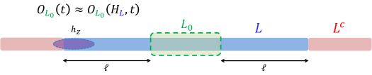
Figure 1: Approximation of the time evolved operator $O_{L_{0}}(t)$ by $O_{L_{0}}(H_{L},t)$, where $L_{0}$ and $L^{\rm c}$ are separated by a distance $\ell$ (Corollary 5). The approximation is derived from Lemma 4 and the Lieb-Robinson bound, where the commutator between $O_{L_{0}}(t)$ and the boundary interaction $h_{Z}$ with $Z\cap L\neq\emptyset$ and $Z\cap L^{\rm c}\neq\emptyset$.

Using the above lemma with the combination of the Lieb-Robinson bound, we can prove the following corollary:

Corollary 5.

Let $\mathcal{F}(r)$ be the Lieb-Robinson bound as

$$\left\|[O_{Z}(t),O_{Z^{\prime}}]\right\|\leq\left\|O_{Z}\right\|\cdot\left\|O_{Z^{\prime}}\right\|\cdot|Z|\cdot|Z^{\prime}|e^{v|t|}\mathcal{F}(r).$$ (39)

Then, under the condition $d_{L^{\rm c},L_{0}}\geq\ell$, the inequality (37) reduces to the following explicit form:

$$\|O_{L_{0}}(H,t)-O_{L_{0}}(H_{L},t)\|\leq|t|\cdot|L_{0}|\cdot\left\|O_{L_{0}}\right\|\left[\frac{g\gamma^{2}\ell^{2}}{4}\bar{J}(\ell/2)+\tilde{g}ke^{v|t|}\mathcal{F}(\ell/2)\right],$$ (40)

where we define $\tilde{g}$ as

$$\tilde{g}:=g\gamma^{2}\bar{J}(1).$$ (41)

Proof of Corollary 5. We start from the inequality (37). We then have to estimate

$$\sum_{Z:Z\in\mathcal{S}_{L}}\int_{0}^{t}\left\|[h_{Z}(H_{L},x),O_{L_{0}}]\right\|dx.$$ (42)

We first decompose

$$\sum_{Z:Z\in\mathcal{S}_{L}}h_{Z}=\sum_{Z:Z\in\mathcal{S}_{L},d_{Z,L_{0}}\leq\ell/2}h_{Z}+\sum_{Z:Z\in\mathcal{S}_{L},d_{Z,L_{0}}>\ell/2}h_{Z}.$$ (43)

Then, from the definition $\mathcal{S}_{L}$ in Eq. (38), we have

$$\sum_{Z:Z\in\mathcal{S}_{L},d_{Z,L_{0}}\leq\ell/2}\left\|h_{Z}\right\|\leq\sum_{Z:Z\cap L^{\rm c}\neq\emptyset,Z\cap L_{1}\neq\emptyset}\left\|h_{Z}\right\|\leq\bar{V}_{L^{\rm c},L_{1}},$$ (44)

where we define the subset $L_{1}$ as $L_{1}:=\{i\in\Lambda|d_{i,L^{\rm c}}>\ell/2\}$ and the upper bound has been defined by Eq. (11), which obeys the upper bound in (10), i.e.,

$$\bar{V}_{L^{\rm c},L_{1}}\leq g\gamma^{2}(\ell/2)^{2}\bar{J}(\ell/2).$$ (45)

We therefore obtain

$$\sum_{Z:Z\in\mathcal{S}_{L},d_{Z,L_{0}}\leq\ell/2}\int_{0}^{t}\left\|[h_{Z}(H_{L},x),O_{L_{0}}]\right\|dx\leq\frac{g\gamma^{2}\ell^{2}}{4}|t|\cdot\left\|O_{L_{0}}\right\|\bar{J}(\ell/2).$$ (46)

For the second term in the RHS of Eq. (43), we use the Lieb-Robinson bound as

$$\left\|[h_{Z}(H_{L},x),O_{L_{0}}]\right\|\leq|Z|\cdot|L_{0}|\cdot\left\|O_{L_{0}}\right\|\cdot\left\|h_{Z}\right\|e^{vx}\mathcal{F}(d_{Z,L_{0}},x)\leq k|L_{0}|\cdot\left\|O_{L_{0}}\right\|\cdot\left\|h_{Z}\right\|e^{v|t|}\mathcal{F}(\ell/2)$$ (47)

for $0\leq x\leq t$ and $d_{Z,L_{0}}>\ell/2$, where we use $|Z|\leq k$. Then, by using

$$\sum_{Z:Z\in\mathcal{S}_{L},d_{Z,L_{0}}>\ell/2}\left\|h_{Z}\right\|\leq\sum_{Z:Z\in\mathcal{S}_{L}}\left\|h_{Z}\right\|=\sum_{Z:Z\cap L\neq\emptyset,Z\cap L^{\rm c}\neq\emptyset}\left\|h_{Z}\right\|=\bar{V}_{L,L^{\rm c}}\leq g\gamma^{2}\bar{J}(1)=:\tilde{g},$$ (48)

we obtain

$$\sum_{\begin{subarray}{c}Z:Z\in\mathcal{S}_{L},d_{Z,L_{0}}>\ell/2\end{subarray}}\int_{0}^{t}\left\|[h_{Z}(H_{L},x),O_{L_{0}}]\right\|dx\leq\tilde{g}k|t|\cdot|L_{0}|\cdot\left\|O_{L_{0}}\right\|e^{v|t|}\mathcal{F}(\ell/2).$$ (49)

By combining the two inequalities (46) and (49), we prove the main inequality (40). This completes the proof. $\square$

III.2 Interaction-truncated Hamiltonian

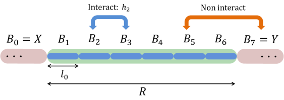
Figure 2: We truncate the Hamiltonian’s interactions by introducing subregions $\{B_{s}\}_{s=0}^{q+1}$ across the system. This leads to the partitioning of the system into $(q+2)$ blocks, with $q=6$ as depicted in the figure. The sequence of blocks $\{B_{s}\}_{s=1}^{q}$ have a length of $l_{0}$, respectively, whereas the terminal blocks $B_{0}$ and $B_{q+1}$ stretch to the left and right extremities of the system, respectively. Following this, we truncate all interactions between these distinct blocks, which ensures the interaction length of at most $2l_{0}$. Then, the truncated Hamiltonian, denoted as $H_{{\rm t}}$ in Eq. (51), remains substantially similar to the original Hamiltonian $H$, as established in Lemma 6. We here consider the open boundary condition, but the same procedure is possible under the periodic boundary (see Ref. [14, Supplementary Figure 6]).

We here adopt the same definition of the interaction-truncated Hamiltonian as in Ref. [14] (see also Fig. 2). We begin by partitioning the total system into blocks: $B_{0}$, $\{B_{s}\}_{s=1}^{q}$, and $B_{q+1}$, satisfying $\bigcup_{s=0}^{q+1}B_{s}=\Lambda$. Here, $q$ is an even integer ($q\geq 2$), and we choose each $B_{s}$ (for $1\leq s\leq q$) such that $|B_{s}|=l_{0}$. The subsets $X$ and $Y$ are defined in terms of these blocks as:

$$X=B_{0},\quad Y=B_{q+1}.$$ (50)

We then truncate all interactions between non-adjacent blocks. After the truncation, only interactions between adjacent blocks remain, leading to the truncated Hamiltonian:

$$H_{\rm t}=\sum_{s=0}^{q+1}v_{s}+\sum_{s=0}^{q}h_{s},\quad v_{s}:=H_{B_{s}},\quad h_{s}:=V_{B_{s},B_{s+1}}(B_{s}\sqcup B_{s+1}),$$ (51)

where we use the definition of $V_{L,L^{\prime}}(\Lambda_{0})$ in Eq. (9) with $X=B_{s}$, $Y=B_{s+1}$, and $\Lambda_{0}=B_{s}\sqcup B_{s+1}$. The term $h_{s}$ denotes the interaction between the blocks $B_{s}$ and $B_{s+1}$. Note that $h_{s}\succeq 0$ is satisfied because of $h_{Z}\succeq 0$. From Lemma 1 with $d_{B_{s},B_{s+1}}=1$, we obtain the upper bound of $h_{s}$ as follows:

$$\left\|h_{s}\right\|=\left\|V_{B_{s},B_{s+1}}(B_{s}\sqcup B_{s+1})\right\|\leq g\gamma^{2}\bar{J}(1)=:\tilde{g}.$$ (52)

Using the following two lemmas, we can derive the inequality of

$$\left\|e^{\beta H}-e^{\beta H_{\rm t}}\right\|_{1} \leq 3\beta\gamma^{2}gql_{0}^{2}\bar{J}(l_{0}){\rm tr}\left(e^{\beta H}\right)$$

$$=\Theta(1)\beta Rl_{0}\bar{J}(l_{0}){\rm tr}\left(e^{\beta H}\right)\quad\textrm{for}\quad\beta\gamma^{2}gql_{0}^{2}\bar{J}(l_{0})\leq 1,$$ (53)

where we use $q\propto R/l_{0}$.

Lemma 6.

Let us adopt the upper bound in Lemma 1. Then, the norm distance between $H$ and $H_{\rm t}$ is bounded from above by

$$\|\delta H_{\rm t}\|\leq\gamma^{2}gql_{0}^{2}\bar{J}(l_{0}),$$ (54)

where we define $\delta H_{\rm t}:=H-H_{\rm t}$. The proof was given in Ref. [14, Supplementary Lemma 3].

Lemma 7.

For arbitrary Hermitian operators $A$ and $B$, we have

$$\left\|e^{A+B}-e^{A}\right\|_{1}\leq\|B\|e^{\left\|B\right\|}\cdot\left\|e^{A}\right\|_{1}.$$ (55)

In particular, if $\|B\|\leq 1$, the above inequality reduces to

$$\left\|e^{A+B}-e^{A}\right\|_{1}\leq 3\|B\|\cdot\left\|e^{A}\right\|_{1}.$$ (56)

Remark. The obtained inequality is better than the trivial inequality as

$$\left\|e^{A+B}-e^{A}\right\|_{1}=\left\|e^{A+B}e^{-A}e^{A}-e^{A}\right\|_{1} \leq\left\|e^{A+B}e^{-A}-1\right\|\cdot\left\|e^{A}\right\|_{1}$$

$$=\left\|\mathcal{T}e^{\int_{0}^{1}e^{\tau A}Be^{-\tau A}d\tau}-1\right\|\cdot\left\|e^{A}\right\|_{1}$$

$$\leq e^{\left\|B\right\|e^{2\left\|A\right\|}}\left\|B\right\|e^{2\left\|A\right\|}\cdot\left\|e^{A}\right\|_{1},$$ (57)

which is meaningful only in the case of $\left\|B\right\|\ll e^{-2\left\|A\right\|}$.

Proof of Lemma 7. We start with the decomposition of

$$e^{A+B}=\Phi_{B}e^{A}\Phi_{B}^{\dagger},$$ (58)

where $\Phi_{B}$ is given by the belief propagation operator [21, 28, 29] (see also Lemma 9 below):

$$\Phi_{B}=\mathcal{T}e^{\int_{0}^{1}\phi_{B,\tau}d\tau},$$

$$\phi_{B,\tau}=\frac{1}{2}\int_{-\infty}^{\infty}f(t)B(A+\tau B,t)dt,$$

$$f(t):=\frac{1}{2\pi}\int_{-\infty}^{\infty}\tilde{f}(\omega)e^{-i\omega t}d\omega,\hskip 10.84006pt\tilde{f}(\omega)=\frac{{\rm tanh}(\omega/2)}{\omega/2},$$ (59)

where $\mathcal{T}$ is the time ordering operator, and we can ensure $f(t)\geq 0$ as in Eq. (71). Hence, we have

$$\left\|\phi_{B,\tau}\right\|\leq\frac{\left\|B\right\|}{2}\int_{-\infty}^{\infty}f(t)dt=\frac{\left\|B\right\|}{2}\tilde{f}(0)=\frac{\left\|B\right\|}{2},$$ (60)

which yields

$$\left\|\Phi_{B}-\hat{1}\right\|\leq e^{\int_{0}^{1}\left\|\phi_{B,\tau}\right\|d\tau}\int_{0}^{1}\left\|\phi_{B,\tau}\right\|d\tau\leq\frac{\left\|B\right\|}{2}e^{\left\|B\right\|/2},$$ (61)

where we use [34, Claim 25 therein] in the first inequality, i.e.,

$$\left\|\mathcal{T}e^{\int_{0}^{1}A_{\tau}d\tau}-\mathcal{T}e^{\int_{0}^{1}B_{\tau}d\tau}\right\|\leq e^{\int_{0}^{1}\max\left(\left\|A_{\tau}\right\|,\left\|B_{\tau}\right\|\right)d\tau}\int_{0}^{1}\left\|A_{\tau}-B_{\tau}\right\|d\tau.$$ (62)

We then obtain

$$\left\|e^{A+B}-e^{A}\right\|_{1}=\left\|\Phi_{B}e^{A}\Phi_{B}^{\dagger}-e^{A}\Phi_{B}^{\dagger}+e^{A}\Phi_{B}^{\dagger}-e^{A}\right\|_{1} \leq\left\|(\Phi_{B}-\hat{1})e^{A}\Phi_{B}^{\dagger}\right\|_{1}+\left\|e^{A}(\Phi_{B}^{\dagger}-\hat{1})\right\|_{1}$$

$$\leq\frac{\left\|B\right\|}{2}e^{\left\|B\right\|/2}\left(1+e^{\left\|B\right\|/2}\right)\left\|e^{A}\right\|_{1}$$

$$\leq\left\|B\right\|e^{\left\|B\right\|}\left\|e^{A}\right\|_{1}.$$ (63)

This completes the proof. $\square$

Under the truncation of the Hamiltonian, the Lieb-Robinson bound (32) is given by the following corollary:

Corollary 8.

For the interaction truncated Hamiltonian (51), the Lieb-Robinson bound is given as follows:

$$\left\|[O_{Z}(H_{\rm t},t),O_{Z^{\prime}}]\right\|\leq\left\|O_{Z}\right\|\cdot\left\|O_{Z^{\prime}}\right\|\cdot|Z|\cdot|Z^{\prime}|e^{v|t|}\mathcal{F}(r),$$ (64)

for $Z,Z^{\prime}\subset B_{1:q}$, where $r=d_{Z,Z^{\prime}}$, and $\mathcal{F}(r)$ is given by

$$\mathcal{F}(r)=C\min\left(e^{-r/(2l_{0})},\bar{J}(r)\right),$$ (65)

where we use the fact that the interaction length is at most $2l_{0}$.

III.3 Quantum belief propagation

We here adopt the interaction-truncated Hamiltonian in the previous section. We omit the index and denote

$$H_{\rm t}\to H$$ (66)

for simplicity. Then, the Hamiltonian has the interaction length of $2l_{0}$ and satisfies the inequality (64).

Also, the belief propagation operator [21, 28, 29] is formulated as follows:

Lemma 9.

Given the decomposition of the Hamiltonian as

$$H=H_{\leq s}+H_{>s}+h_{s},$$ (67)

we obtain

$$e^{\beta H}=\Phi_{s}e^{\beta(H_{\leq s}+H_{>s})}\Phi_{s}^{\dagger},$$ (68)

where the explicit expression of the belief propagation operator $\Phi_{s}$ is given as follows:

$$\Phi_{s} =\mathcal{T}e^{\int_{0}^{1}\phi_{s,\tau}d\tau},$$ (69)

$$\phi_{s,\tau} =\frac{\beta}{2}\int_{-\infty}^{\infty}f_{\beta}(t)h_{s}(H_{\tau},t)dt.$$

Here, $\mathcal{T}$ represents the time ordering operator, $H_{\tau}:=H_{\leq s}+H_{>s}+\tau h_{s}$, and the function $f_{\beta}(t)$ is defined as follows:

$$f_{\beta}(t):=\frac{1}{2\pi}\int_{-\infty}^{\infty}\tilde{f}_{\beta}(\omega)e^{-i\omega t}d\omega,\hskip 10.84006pt\tilde{f}(\omega)=\frac{{\rm tanh}(\beta\omega/2)}{\beta\omega/2}.$$ (70)

The function $f_{\beta}(t)$ has been explicitly computed as follows [33]:

$$f_{\beta}(t)=\frac{2}{\pi\beta}\log\left(\frac{e^{\pi|t|/\beta}+1}{e^{\pi|t|/\beta}-1}\right)\leq\frac{2}{\pi\beta}\frac{2}{e^{\pi|t|/\beta}-1}.$$ (71)

Because of $f_{\beta}(t)\geq 0$ and

$$\int_{-\infty}^{\infty}|f_{\beta}(t)|dt=\tilde{f}(\omega=0)=1,$$ (72)

we have

$$\left\|\phi_{s,\tau}\right\|\leq\frac{\beta}{2}\int_{-\infty}^{\infty}f_{\beta}(t)\left\|h_{s}(H_{\tau},t)\right\|dt\leq\frac{\beta\left\|h_{s}\right\|}{2}\leq\frac{\beta\tilde{g}}{2},$$ (73)

where we use the inequality (52), i.e., $\left\|h_{s}\right\|\leq\tilde{g}$. The above inequality immediately gives

$$\left\|\Phi_{s}\right\| \leq e^{\int_{0}^{1}\left\|\phi_{s,\tau}\right\|d\tau}\leq e^{\beta\tilde{g}/2}.$$ (74)

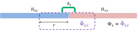
Figure 3: The quantum belief propagation operator $\Phi_{s}$ characterizes the transformation from $e^{\beta H_{\leq s}}\otimes e^{\beta H_{>s}}$ to $e^{\beta H}$. It is defined by using the time evolution with respect to $H_{\tau}:=H_{\leq s}+H_{>s}+\tau h_{s}$. The Lieb-Robinson bound ensures the quasi-locality of $\Phi_{s}$ around the boundary as shown in Proposition 10.

We then consider the approximate belief propagation operator $\tilde{\Phi}_{s,\tilde{L}}$ onto a region given by $[s-r,s+r]$ (see Fig. 3), where $\tilde{\Phi}_{s,\tilde{L}}$ is defined by using the subset Hamiltonian $H_{\tilde{L}}$ with $\tilde{L}=[s-r,s+r]$ as follows:

$$\tilde{\Phi}_{s,\tilde{L}}:=\mathcal{T}e^{\int_{0}^{1}\tilde{\phi}_{s,\tau}d\tau},\quad\tilde{\phi}_{s,\tau} =\frac{\beta}{2}\int_{-\infty}^{\infty}f_{\beta}(t)h_{s}\left(H_{\tau,\tilde{L}},t\right)dt.$$ (75)

where $H_{\tau,\tilde{L}}:=H_{[s-r,s]}+H_{(s,s+r]}+\tau h_{s}$ which is supported on the region $\tilde{L}$. We note that the same inequalities as (73) and (74) hold for $\left\|\tilde{\Phi}_{s,\tilde{L}}\right\|$ and $\left\|\phi_{s,\tau}\right\|$. The error between the belief propagation operator $\Phi_{s}$ and the truncated operator $\tilde{\Phi}_{s,\tilde{L}}$, $\left\|\Phi_{s}-\tilde{\Phi}_{s,\tilde{L}}\right\|$, has an upper bound as a function of $r$, denoted by $\mathcal{G}_{\beta}(r)$:

$$\left\|\Phi_{s}-\tilde{\Phi}_{s,\tilde{L}}\right\|\leq\mathcal{G}_{\beta}(r).$$ (76)

The form of $\mathcal{G}_{\beta}(r)$ is estimated by combining the Lieb-Robinson bound and the form of the quantum belief propagation operator:

Proposition 10.

On the approximation between $\Phi_{s}$ and $\tilde{\Phi}_{s,\tilde{L}}$, we prove the upper bound of

$$\left\|\Phi_{s}-\tilde{\Phi}_{s,\tilde{L}}\right\| \leq e^{\beta\tilde{g}/2}\left\{\beta g\gamma^{2}r^{2}\left(1+\frac{k\tilde{g}\beta}{2\pi^{3}}\right)\bar{J}(r/3)+\frac{k\tilde{g}\beta^{2}}{2\pi^{3}}\left[9\tilde{g}\sqrt{\mathcal{F}(r/3)}+72\tilde{g}\left[\mathcal{F}(r/3)\right]^{\pi/(4v\beta)}\right]\right\}$$

$$\leq e^{\Theta(\beta)}\left[r^{2}\bar{J}(r/3)+\left[\mathcal{F}(r/3)\right]^{1/\Theta(\beta)}\right],$$ (77)

where we use the $\Theta$ notation in Eq. (7). In particular, if the interaction length $2l_{0}$ is smaller than $r/3$, i.e.,

$$r>6l_{0},$$ (78)

we prove

$$\mathcal{G}_{\beta}(r) =e^{\beta\tilde{g}/2}\frac{k\tilde{g}\beta^{2}}{2\pi^{3}}\left[9\tilde{g}\sqrt{\mathcal{F}(r/3)}+72\tilde{g}\left[\mathcal{F}(r/3)\right]^{\pi/(4v\beta)}\right]$$

$$\leq e^{\Theta(\beta)}\left[\mathcal{F}(r/3)\right]^{1/\Theta(\beta)}$$

$$=e^{\Theta(\beta)}\min\left(e^{-r/\Theta(\beta l_{0})},\left[\bar{J}(r/3)\right]^{1/\Theta(\beta)}\right),$$ (79)

where we use the Lieb-Robinson bound in (64). Therefore, the function $\mathcal{G}_{\beta}(r)$ is given in the form of

$$\mathcal{G}_{\beta}(r)=e^{\Theta(\beta)}\min\left(e^{-r/\Theta(\beta l_{0})},\left[\bar{J}(r/3)\right]^{1/\Theta(\beta)}\right).$$ (80)

III.3.1 Proof of Proposition 10.

It is enough to derive the upper bound of

$$\left\|\phi_{s,\tau}-\tilde{\phi}_{s,\tau}\right\|$$ (81)

and use the inequality (62). We then obtain

$$\left\|\Phi_{s}-\tilde{\Phi}_{s,\tilde{L}}\right\|\leq e^{\beta\tilde{g}/2}\int_{0}^{1}\left\|\phi_{s,\tau}-\tilde{\phi}_{s,\tau}\right\|d\tau,$$ (82)

where we use $\max(\left\|\phi_{s,\tau}\right\|,\left\|\tilde{\phi}_{s,\tau}\right\|)\leq\beta\tilde{g}/2$.

We first approximate $h_{s}$ onto the region $[s-r/3,s+r/3]$ and define the approximated interaction by $h_{s,r/3}$. Then, the approximation error gives

$$\left\|h_{s}-h_{s,r/3}\right\|\leq\left\|\bar{V}_{(-\infty,s-r/3),[s,\infty)}\right\|+\left\|\bar{V}_{(-\infty,s],(s+r/3,\infty)}\right\|\leq\frac{2g\gamma^{2}r^{2}}{9}\bar{J}(r/3),$$ (83)

where we use the notation $\overline{V}_{L,L^{\prime}}$ in Eq. (11) and the upper bound (10), which holds for $\overline{V}_{L,L^{\prime}}$ as well as for $\|V_{L,L^{\prime}}(\Lambda_{0})\|$. Therefore, by denoting $\phi_{s,\tau}$ and $\tilde{\Phi}^{\prime}_{s,\tilde{L}}$ by

$$\phi^{\prime}_{s,\tau}=\frac{\beta}{2}\int_{-\infty}^{\infty}f_{\beta}(t)h_{s,r/3}(H_{\tau},t)dt,\quad\tilde{\phi}^{\prime}_{s,\tau,r}=\frac{\beta}{2}\int_{-\infty}^{\infty}f_{\beta}(t)h_{s,r/3}(H_{\tau,\tilde{L}},t)dt$$ (84)

with $\tilde{L}=[s-r,s+r]$, we have

$$\left\|\phi_{s,\tau}-\phi^{\prime}_{s,\tau}\right\|\leq\frac{\beta}{2}\int_{-\infty}^{\infty}f_{\beta}(t)\left\|h_{s}-h_{s,r/3}\right\|dt=\frac{\beta g\gamma^{2}r^{2}}{9}\bar{J}(r/3),$$ (85)

where we use Eq. (72) in the last equation. The same inequality holds for $\left\|\tilde{\phi}_{s,\tau}-\tilde{\phi}^{\prime}_{s,\tau,r}\right\|$, where $\tilde{\phi}_{s,\tau}$ has been defined in Eq. (75).

We then consider

$$\left\|\phi^{\prime}_{s,\tau}-\tilde{\phi}^{\prime}_{s,\tau}\right\|\leq\frac{\beta}{2}\int_{-\infty}^{\infty}f_{\beta}(t)\left\|h_{s,r/3}(H_{\tau},t)-h_{s,r/3}(H_{\tau,\tilde{L}},t)\right\|dt.$$ (86)

For this purpose, we upper-bound

$$\left\|h_{s,r/3}(H_{\tau},t)-h_{s,r/3}(H_{\tau,\tilde{L}},t)\right\|\leq\sum_{\begin{subarray}{c}Z:Z\subseteq[s-r/3,s+r/3]\\ Z\cap(-\infty,s]\neq\emptyset,Z\cap(s,\infty)\neq\emptyset\end{subarray}}\left\|h_{Z}(H_{\tau},t)-h_{Z}(H_{\tau,\tilde{L}},t)\right\|.$$ (87)

Because of $d_{Z,L^{\rm c}}\geq 2r/3$, we use Corollary 5 to obtain

$$\left\|h_{Z}(H_{\tau},t)-h_{Z}(H_{\tau,\tilde{L}},t)\right\|\leq|t|k\left\|h_{Z}\right\|\left[\frac{g\gamma^{2}r^{2}}{9}\bar{J}(r/3)+\tilde{g}e^{v|t|}\mathcal{F}(r/3)\right],$$ (88)

which reduces the inequality (87) to

$$\left\|h_{s,r/3}(H_{\tau},t)-h_{s,r/3}(H_{\tau,\tilde{L}},t)\right\|\leq|t|k\tilde{g}\left[\frac{g\gamma^{2}r^{2}}{9}\bar{J}(r/3)+\tilde{g}e^{v|t|}\mathcal{F}(r/3)\right],$$ (89)

where we use the inequality (52). We thus obtain

$$\left\|\phi^{\prime}_{s,\tau}-\tilde{\phi}^{\prime}_{s,\tau}\right\|\leq\frac{\beta}{2}\int_{-\infty}^{\infty}f_{\beta}(t)|t|k\tilde{g}\left[\frac{g\gamma^{2}r^{2}}{9}\bar{J}(r/3)+\tilde{g}e^{v|t|}\mathcal{F}(r/3)\right]dt.$$ (90)

We finally calculate the time integration in Eq. (90). From the definition (71), we have

$$\int_{-\infty}^{\infty}|t|f_{\beta}(t)dt=\frac{4\beta}{\pi^{3}}\int_{0}^{\infty}x\log\left(\frac{e^{x}+1}{e^{x}-1}\right)dx=\frac{7\zeta(3)\beta}{\pi^{3}},$$ (91)

where $\zeta(x)$ is the Riemann’s zeta function. We next consider

$$\int_{-\infty}^{\infty}|t|f_{\beta}(t)e^{v|t|}\mathcal{F}(r/3)dt =2\int_{0}^{\infty}tf_{\beta}(t)e^{v|t|}\mathcal{F}(r/3)dt$$

$$=2\int_{0}^{t_{0}}tf_{\beta}(t)e^{v|t|}\mathcal{F}(r/3)dt+2\int_{t_{0}}^{\infty}tf_{\beta}(t)e^{v|t|}\mathcal{F}(r/3)dt,$$ (92)

where we choose $t_{0}$ such that for $t\leq t_{0}$

$$e^{vt}\mathcal{F}(r/3)\leq\sqrt{\mathcal{F}(r/3)}\longrightarrow t_{0}=\frac{-1}{2v}\log\left[\mathcal{F}(r/3)\right].$$ (93)

We then obtain

$$2\int_{0}^{t_{0}}tf_{\beta}(t)e^{v|t|}\mathcal{F}(r/3)dt\leq 2\sqrt{\mathcal{F}(r/3)}\int_{0}^{\infty}tf_{\beta}(t)dt=\frac{7\zeta(3)\beta}{\pi^{3}}\sqrt{\mathcal{F}(r/3)},$$ (94)

and

$$2\int_{t_{0}}^{\infty}tf_{\beta}(t)e^{v|t|}\mathcal{F}(r/3)dt\leq 4\int_{t_{0}}^{\infty}tf_{\beta}(t)dt \leq 4e^{-\pi t_{0}/(2\beta)}\int_{t_{0}}^{\infty}te^{\pi t/(2\beta)}f_{\beta}(t)dt$$

$$\leq\frac{72\beta}{\pi^{3}}\left[\mathcal{F}(r/3)\right]^{\pi/(4v\beta)},$$ (95)

where we use the trivial bound (33) and

$$\int_{0}^{\infty}te^{\pi t/(2\beta)}f_{\beta}(t)dt=\frac{2\beta}{\pi^{3}}\int_{0}^{\infty}xe^{x/2}\log\left(\frac{e^{x}+1}{e^{x}-1}\right)dx\leq\frac{18\beta}{\pi^{3}}.$$ (96)

By applying the inequalties (94) and (III.3.1) to Eq. (III.3.1), we obtain

$$\int_{-\infty}^{\infty}|t|f_{\beta}(t)e^{v|t|}\mathcal{F}(r/3)dt \leq\frac{\beta}{\pi^{3}}\left(7\zeta(3)\sqrt{\mathcal{F}(r/3)}+72\left[\mathcal{F}(r/3)\right]^{\pi/(4v\beta)}\right),$$ (97)

which reduces the inequality (90) to

$$\left\|\phi^{\prime}_{s,\tau}-\tilde{\phi}^{\prime}_{s,\tau}\right\| \leq\frac{k\tilde{g}\beta^{2}}{2\pi^{3}}\left[\frac{7\zeta(3)g\gamma^{2}r^{2}}{9}\bar{J}(r/3)+\tilde{g}\left(7\zeta(3)\sqrt{\mathcal{F}(r/3)}+72\left[\mathcal{F}(r/3)\right]^{\pi/(4v\beta)}\right)\right]$$

$$\leq\frac{k\tilde{g}\beta^{2}}{2\pi^{3}}\left[g\gamma^{2}r^{2}\bar{J}(r/3)+9\tilde{g}\sqrt{\mathcal{F}(r/3)}+72\tilde{g}\left[\mathcal{F}(r/3)\right]^{\pi/(4v\beta)}\right].$$ (98)

By combining the above bound with (85), we finally arrive at the inequality

$$\left\|\phi_{s,\tau}-\tilde{\phi}_{s,\tau}\right\| \leq\left\|\phi_{s,\tau}-\phi^{\prime}_{s,\tau}\right\|+\left\|\tilde{\phi}_{s,\tau}-\tilde{\phi}^{\prime}_{s,\tau}\right\|+\left\|\phi^{\prime}_{s,\tau}-\tilde{\phi}^{\prime}_{s,\tau}\right\|$$

$$\leq\frac{2\beta g\gamma^{2}r^{2}}{9}\bar{J}(r/3)+\frac{k\tilde{g}\beta^{2}}{2\pi^{3}}\left[g\gamma^{2}r^{2}\bar{J}(r/3)+9\tilde{g}\sqrt{\mathcal{F}(r/3)}+72\tilde{g}\left[\mathcal{F}(r/3)\right]^{\pi/(4v\beta)}\right].$$ (99)

We thus prove the main inequality (10) from the inequality (82).

Under the condition (78), we ensure $\left\|\phi_{s,\tau}-\phi^{\prime}_{s,\tau}\right\|=\left\|\tilde{\phi}_{s,\tau}-\tilde{\phi}^{\prime}_{s,\tau,r}\right\|=0$ in (85), which reduces the above inequality to the form of (10). This completes the proof. $\square$

IV Cluster expansion technique

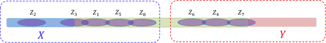
Figure 4: An image displaying the decomposition of the collection of sets $\{X,Z_{1},Z_{2},\ldots,Z_{8},Y\}$ into two disjoint subcollections, $\{X,Z_{1},Z_{2},Z_{3},Z_{5},Z_{8}\}$ and $\{Z_{4},Z_{6},Z_{7},R\}$, is shown. When the sets, $Z_{1}$, $Z_{2}$, $\ldots$, $Z_{8}$, cannot connect the distant regions $L$ and $R$, the trace vanishes.

In proving the clustering theorem, we utilize the cluster expansion technique. We first rewrite an arbitrary bi-partite correlation function ${\rm Cor}_{\rho_{\beta}}(O_{X},O_{Y})$ as follows [39]:

$${\rm Cor}_{\rho_{\beta}}(O_{X},O_{Y})={\rm tr}\left(\rho_{\beta}\otimes\rho_{\beta}O_{X}^{(0)}O_{Y}^{(1)}\right)=\frac{1}{Z_{\beta}^{(+)}}{\rm tr}\left(e^{\beta H^{(+)}}O_{X}^{(0)}O_{Y}^{(1)}\right),$$ (100)

where the operators $O^{(+)}$, $O^{(0)}$ and $O^{(1)}$ are defined by adopting a copy of the original Hilbert space:

$$O^{(+)}=O\otimes\hat{1}+\hat{1}\otimes O,\quad O^{(0)}=O\otimes\hat{1},\quad O^{(1)}=O\otimes\hat{1}-\hat{1}\otimes O.$$ (101)

One can easily check that Eq. (100) holds. Then, the following lemma holds:

Lemma 11.

For an arbitrary set of operators $\{O_{Z_{j}}\}_{j=1}^{m}$, the following relation holds:

$${\rm tr}\left(O_{Z_{1}}^{(+)}O_{Z_{2}}^{(+)}\cdots O_{Z_{m}}^{(+)}O_{X}^{(0)}O_{Y}^{(1)}\right)=0,$$ (102)

when the subsets $\{X,Z_{1},Z_{2},\ldots,Z_{m},Y\}$ are not connected (see Fig. 4); that is there exists a decomposition of $\{1,2,\ldots,m\}=\{i_{1},i_{2},\ldots,i_{s}\}\oplus\{i_{s+1},i_{s+2},\ldots,i_{m}\}$ such that

$$\left(X\cup Z_{i_{1}}\cup Z_{i_{2}}\cup\cdots\cup Z_{i_{s}}\right)\cap\left(Y\cup Z_{i_{s+1}}\cup Z_{i_{s+2}}\cup\cdots\cup Z_{i_{m}}\right)=\emptyset.$$ (103)

Proof of Lemma 11. By assumption, the collection of sets, $\{X,Z_{1},\ldots,Z_{m},Y\}$, decomposes into two subcollections of sets:

$$\mathcal{C}_{1} =\{X,Z_{i_{1}},\ldots,Z_{i_{s}}\},$$ (104)

$$\mathcal{C}_{2} =\{Y,Z_{i_{s+1}},\ldots,Z_{i_{m}}\},$$

such that the union of the sets in the subcollection $\mathcal{C}_{1}$ and the union of the sets in the subcollection $\mathcal{C}_{2}$ are disjoint, as in the relation (103). This means that the trace

$${\rm tr}\left(O^{(+)}_{Z_{1}}O^{(+)}_{Z_{2}}\ldots O^{(+)}_{Z_{m}}O^{(0)}_{X}O^{(1)}_{Y}\right)$$ (105)

can be rewritten by the product as the following:

$${\rm tr}\left(O^{(+)}_{Z_{1}}O^{(+)}_{Z_{2}}\ldots O^{(+)}_{Z_{m}}O^{(0)}_{X}O^{(1)}_{Y}\right)={\rm tr}\left(\prod_{j=1}^{s}O^{(+)}_{Z_{i_{j}}}\cdot O^{(0)}_{X}\right)\,{\rm tr}\left(O^{(1)}_{Y}\prod_{k=s+1}^{m}O^{(+)}_{Z_{i_{k}}}\right).$$ (106)

However, the operators $O^{(+)}_{Z_{i_{k}}}=O_{Z_{i_{k}}}\otimes\hat{1}+\hat{1}\otimes O_{Z_{i_{k}}}$ are symmetric while the operator $O^{(1)}_{Y}=O_{Y}\otimes\hat{1}-\hat{1}\otimes O_{Y}$ is antisymmetric for the exchange between the two Hilbert spaces. Owing to these properties of the operators, we have the following equality:

$${\rm tr}\left(O^{(1)}_{Y}\prod_{k=s+1}^{m}O^{(+)}_{Z_{i_{k}}}\right)={\rm tr}\left(O_{Y}\otimes\hat{1}\cdot\prod_{k=s+1}^{m}O^{(+)}_{Z_{i_{k}}}\right)-{\rm tr}\left(\hat{1}\otimes O_{Y}\cdot\prod_{k=s+1}^{m}O^{(+)}_{Z_{i_{k}}}\right)=0.$$ (107)

This shows that the trace (105) vanishes under the assumption. This completes the proof. $\square$

By using Lemma 11, the function ${\rm Cor}_{\rho_{\beta}}(O_{X},O_{Y})$ can be expanded as

$${\rm Cor}_{\rho_{\beta}}(O_{X},O_{Y})=\frac{1}{Z_{\beta}^{(+)}}\sum_{m=0}^{\infty}\sum_{Z_{1},Z_{2},\ldots,Z_{m}:{\rm connected}}\frac{1}{m!}{\rm tr}\left(h_{Z_{1}}^{(+)}h_{Z_{2}}^{(+)}\cdots h_{Z_{m}}^{(+)}O_{X}^{(0)}O_{Y}^{(1)}\right),$$ (108)

where the summation $\sum_{Z_{1},Z_{2},\ldots,Z_{m}:{\rm connected}}$ is taken over the collections $\{X,Z_{1},Z_{2},\ldots,Z_{m},Y\}$ that connect $L$ and $R$. We then define the operator $\rho_{{\rm cl}}$ as follows:

$$\rho_{{\rm cl}}:=\frac{1}{Z_{\beta}^{(+)}}\sum_{m=0}^{\infty}\sum_{Z_{1},Z_{2},\ldots,Z_{m}:{\rm connected}}\frac{\beta^{m}}{m!}h_{Z_{1}}^{(+)}h_{Z_{2}}^{(+)}\cdots h_{Z_{m}}^{(+)}.$$ (109)

Using the operator $\rho_{{\rm cl}}$, the bi-parite correlation ${\rm Cor}_{\rho_{\beta}}(O_{X},O_{Y})$ has the following upper bound:

$${\rm Cor}_{\rho_{\beta}}(O_{X},O_{Y})\leq\left\|O_{X}\right\|\cdot\left\|O_{Y}\right\|\cdot\left\|\rho_{{\rm cl}}\right\|_{1}.$$ (110)

A standard counting (e.g., in Refs. [43, 44]) gives an upper bound on the summand in Eq. (109) as

$$\frac{1}{Z_{\beta}^{(+)}}\sum_{Z_{1},Z_{2},\ldots,Z_{m}:{\rm connected}}\frac{1}{m!}\left\|h_{Z_{1}}^{(+)}h_{Z_{2}}^{(+)}\cdots h_{Z_{m}}^{(+)}\right\|\lesssim\left(\beta/\beta_{c}\right)^{m},$$ (111)

where $\beta_{c}$ is an $\mathcal{O}(1)$ constant. The upper bound on the RHS of (111) summed over $m$ converges only when the value of $\beta$ is less than the threshold value, $\beta_{c}$, i.e. only when $\beta<\beta_{c}$. Therefore, the use of this upper bound ensures that the summation in $\rho_{{\rm cl}}$ converges to a finite value only for $\beta<\beta_{c}$. This limitation yields the main challenge in proving the clustering theorem in a 1D system at arbitrary temperatures. Thus, we have to avoid this argument for temperatures higher than the threshold value $\beta_{c}$.

In the following, we focus on the cluster expansion in 1D finite-range interacting systems as in Eq. (51). We adopt the operator $\Psi_{X,Y}$ as

$$\Psi_{X,Y}:=O_{X}^{(0)}O_{Y}^{(1)},\quad\left\|\Psi_{X,Y}\right\|\leq 2,$$ (112)

where in the inequality, we use $\left\|O_{X}^{(0)}\right\|\leq\left\|O_{X}\right\|=1$ and $\left\|O_{Y}^{(1)}\right\|=\left\|O_{Y}\otimes\hat{1}-\hat{1}\otimes O_{Y}\right\|\leq 2\left\|O_{Y}\right\|=2$. Moreover, for simplicity of the notation, we denote

$$H_{\rm t}\to H,\quad H^{(+)}\to H,\quad Z_{\beta}^{(+)}\to Z_{\beta}$$ (113)

by omitting the indices.

Then, if one of the interaction terms $\{h_{s}\}_{s=0}^{q}$ has zeroth order in the Taylor expansion of $e^{\beta H}$, the cluster is unconnected. To mathematically characterize it, we define the operator

$$G_{j}:=e^{\beta H}-e^{\beta(H-h_{s})}=-\int_{0}^{1}\frac{d}{d\lambda_{s}}e^{\beta H-\beta\lambda_{s}h_{s}}d\lambda_{s}.$$ (114)

Then, the operator $G_{j}$ removes the zeroth-order term of $h_{s}$ from the Taylor expansion of $e^{\beta H}$. This generalizes to situations involving multiple parameters. In the case of multi-parameters, we define

$$G_{s_{1},s_{2},\ldots,s_{m}} :=(-1)^{m}\int_{0}^{1}\int_{0}^{1}\cdots\int_{0}^{1}d\lambda_{s_{1}}d\lambda_{s_{2}}\cdots d\lambda_{s_{m}}\frac{d}{d\lambda_{s_{1}}}\frac{d}{d\lambda_{s_{2}}}\cdots\frac{d}{d\lambda_{s_{m}}}e^{\beta H-\beta\sum_{j=1}^{m}\lambda_{s}h_{s_{j}}}$$

$$=\mathcal{D}_{h_{s_{1}},\ldots,h_{s_{m}}}e^{\beta H}.$$ (115)

The super-operator $\mathcal{D}_{h_{s_{1}},\ldots,h_{s_{m}}}$ removes all zeroth-order terms of $h_{s_{j}}$ ($j=1,\ldots,m$) from the Taylor expansion of $e^{\beta H}$. Using Lemma 11, we can obtain

$${\rm tr}\left[\Psi_{X,Y}\left(\rho_{\beta}-G_{s_{1},s_{2},\ldots,s_{m}}\right)\right]=0$$ (116)

for arbitrary sets of $\{s_{1},s_{2},\ldots,s_{m}\}$, which also yields

$${\rm Cor}_{\rho_{\beta}}(O_{X},O_{Y})\leq\frac{1}{Z_{\beta}}\left|{\rm tr}\left(\Psi_{X,Y}G_{s_{1},s_{2},\ldots,s_{m}}\right)\right|\leq\frac{2}{Z_{\beta}}\left\|G_{s_{1},s_{2},\ldots,s_{m}}\right\|_{1}.$$ (117)

Thus, upper-bounding the norm of $\left\|G_{s_{1},s_{2},\ldots,s_{m}}\right\|_{1}$ yields the clustering theorem.

IV.1 1D cases: commuting Hamiltonian

We demonstrate the commutative situation here, i.e., $[h_{s},h_{s^{\prime}}]=0$ for $\forall s,s^{\prime}\in[0,q]$ in Eq. (51). The aforementioned restriction on values of $\beta$ does not arise in this simple scenario. Comparing the commutative and noncommutative situations allows for a clear identification of the challenges that arise in proving the clustering theorem. The challenges for noncommutative situations will be identified afterward.

In the commuting cases, the operation $\mathcal{D}_{h_{s_{1}},\ldots,h_{s_{m}}}$ in Eq. (IV) simply implies the replacement of $e^{\beta h_{s_{1}}}$ with $e^{\beta h_{s_{1}}}-\hat{1}$ in the Gibbs state

$$e^{\beta H}=\prod_{s=0}^{q+1}e^{\beta v_{s}}\prod_{s=0}^{q}e^{\beta h_{s}},$$ (118)

where we use the notation of Eq. (51). We then estimate the trace norm of $\left\|G_{0,1,\ldots,q}\right\|_{1}$ simply by the trace of $G_{0,1,\ldots,q}$ as

$$\left\|G_{0,1,\ldots,q}\right\|_{1}={\rm tr}\left(G_{0,1,\ldots,q}\right)={\rm tr}\left[\prod_{s=0}^{q+1}e^{\beta v_{s}}\prod_{s=0}^{q}\left(e^{\beta h_{s}}-\hat{1}\right)\right].$$ (119)

Note that the positivity of the operator $\left(e^{\beta h_{s}}-\hat{1}\right)$ is ensured by $h_{s}\succeq 0$.

To see the point, it is useful to observe that the following inequality holds in the first step:

$${\rm tr}\left[e^{\beta H-\beta h_{0}}\left(e^{\beta h_{0}}-\hat{1}\right)\right]={\rm tr}\left(e^{\beta H}\right)\cdot\frac{{\rm tr}\left[e^{\beta H-\beta h_{0}}\left(e^{\beta h_{0}}-\hat{1}\right)\right]}{{\rm tr}\left(e^{\beta H-\beta h_{0}}e^{\beta h_{0}}\right)}\leq{\rm tr}\left(e^{\beta H}\right)\cdot\frac{e^{\beta||h_{0}||}-1}{e^{\beta||h_{0}||}},$$ (120)

where the last inequality holds owing to the following inequality for any quantum state $\rho$:

$$\frac{{\rm tr}\left[\rho(e^{\beta h_{0}}-\hat{1})\right]}{{\rm tr}\left(\rho e^{\beta h_{0}}\right)}\leq\frac{e^{\beta||h_{0}||}-1}{e^{\beta||h_{0}||}}.$$ (121)

In the second step, the same procedure yields the following inequality:

$${\rm tr}\left[e^{\beta(H-h_{0}-h_{1})}\left(e^{\beta h_{0}}-\hat{1}\right)\left(e^{\beta h_{1}}-\hat{1}\right)\right] ={\rm tr}\left[e^{\beta(H-h_{0})}\left(e^{\beta h_{0}}-\hat{1}\right)\right]\cdot\frac{{\rm tr}\left[e^{\beta(H-h_{0}-h_{1})}\left(e^{\beta h_{0}}-\hat{1}\right)\left(e^{\beta h_{1}}-\hat{1}\right)\right]}{{\rm tr}\left[e^{\beta(H-h_{0}-h_{1})}\left(e^{\beta h_{0}}-\hat{1}\right)e^{\beta h_{1}}\right]}$$

$$\leq{\rm tr}\left[e^{\beta(H-h_{0})}\left(e^{\beta h_{0}}-\hat{1}\right)\right]\cdot\frac{e^{\beta||h_{1}||}-1}{e^{\beta||h_{1}||}}$$

$$\leq{\rm tr}\left(e^{\beta H}\right)\cdot\frac{e^{\beta||h_{0}||}-1}{e^{\beta||h_{0}||}}\cdot\frac{e^{\beta||h_{1}||}-1}{e^{\beta||h_{1}||}},$$ (122)

where in the first inequality, we use the fact that $e^{\beta(H-h_{0}-h_{1})}\left(e^{\beta h_{0}}-\hat{1}\right)$ is still positive semidefinite since $e^{\beta h_{0}}-\hat{1}\succeq 0$. In an analogous manner, one deduces after an iteration of this method the following relation:

$${\rm tr}\left[\prod_{s=0}^{q+1}e^{\beta v_{s}}\prod_{s=0}^{q}\left(e^{\beta h_{s}}-\hat{1}\right)\right]\leq{\rm tr}\left(e^{\beta H}\right)\cdot\prod_{s=0}^{q}\frac{e^{\beta||h_{s}||}-1}{e^{\beta||h_{s}||}}.$$ (123)

From the inequality (117), we obtain the upper bound of

$${\rm Cor}_{\rho_{\beta}}(O_{X},O_{Y})\leq 2\prod_{s=0}^{q}\frac{e^{\beta||h_{s}||}-1}{e^{\beta||h_{s}||}}.$$ (124)

In (52), we have obtained

$$||h_{s}||\leq\tilde{g},$$ (125)

and hence, we obtain

$${\rm Cor}_{\rho_{\beta}}(O_{X},O_{Y})\leq 2\prod_{s=0}^{q}\frac{e^{\beta\tilde{g}}-1}{e^{\beta\tilde{g}}} =2\left(1-e^{-\beta\tilde{g}}\right)^{q+1}\leq 2e^{-R/\left(l_{0}e^{\beta\tilde{g}}\right)},$$ (126)

where we use $q=R/l_{0}$ as has been defined in Sec. III.2 and

$$1-\frac{1}{x}\leq e^{-\frac{1}{x}}\quad\textrm{for}\quad x>0.$$ (127)

We thus conclude that this proves the clustering theorem for the commutative case with the correlation length of $l_{0}e^{\beta\tilde{g}}$. When the interaction length $l_{0}$ is an $\mathcal{O}(1)$ constant, the correlation length is given by $e^{\mathcal{O}(\beta)}$.

In extending this discussion to the noncommuting Hamiltonian, we need to overcome the following problems. To make the discussion clear, we consider the operator $G_{s_{1},s_{2}}$ in Eq. (IV), which is given by

$$G_{s_{1},s_{2}}=e^{\beta H}-e^{\beta(H-h_{s_{1}})}-e^{\beta(H-h_{s_{2}})}+e^{\beta(H-h_{s_{1}}-h_{s_{2}})}.$$ (128)

Then, the first difficulty arises from

$$e^{\beta H}-e^{\beta(H-h_{s_{1}})}-e^{\beta(H-h_{s_{2}})}+e^{\beta(H-h_{s_{1}}-h_{s_{2}})}\neq e^{\beta(H-h_{s_{1}}-h_{s_{2}})}\left(1-e^{\beta h_{s_{1}}}\right)\left(1-e^{\beta h_{s_{2}}}\right)$$ (129)

because of the non-commutativity of the operators $h_{s_{1}}$ and $h_{s_{2}}$. This point prohibits us from utilizing the prescription as in (IV.1).

The second difficulty arises from the fact that in general, we have

$$|G_{s_{1},s_{2}}|\neq G_{s_{1},s_{2}}$$ (130)

only from the positivity of $h_{s_{1}}$ and $h_{s_{2}}$. In details, we can ensure

$$e^{\beta H}-e^{\beta H-\beta(h_{s_{1}}+\zeta)}\succeq 0$$ (131)

only when $\zeta$ is sufficiently larger than $\left\|H\right\|=\mathcal{O}(|\Lambda|)$ instead of $\left\|h\right\|$. In general, we can only prove the following lemma:

Lemma 12.

If $A\succeq 0$ and $B\succeq 0$, we have

$$e^{A+B+\zeta}-e^{A}\succeq 0$$ (132)

for $\zeta\geq\left\|A\right\|$.

Proof. $e^{A+B+\zeta}-e^{A}$ can be rewritten as follows:

$$e^{A+B+\zeta}-e^{A}=e^{A/2}\left(e^{-A/2+\zeta/2}e^{A+B}e^{-A/2+\zeta/2}-1\right)e^{A/2}.$$ (133)

Our goal is to prove the positivity of the operator $e^{-A/2+\zeta/2}e^{A+B}e^{-A/2+\zeta/2}-1$. First, from $A+B\succeq 0$, for an arbitrary normalized quantum state $\ket{\psi}$ (i.e., $\left\|\ket{\psi}\right\|=1$), we have $\bra{\psi}e^{A+B}\ket{\psi}\geq 1$. Second, for an arbitrary normalized quantum state $\ket{\phi}$, the state $\ket{\tilde{\phi}}:=e^{-A/2+\zeta/2}\ket{\phi}$ satisfies $\left\|\ket{\tilde{\phi}}\right\|\geq 1$ because of $-A+\zeta\hat{1}\succeq 0$ from $\zeta\geq\left\|A\right\|$. Therefore, by combining the two statements above, we have $\bra{\phi}e^{-A/2+\zeta/2}e^{A+B}e^{-A/2+\zeta/2}\ket{\phi}\geq 1$. This completes the proof. $\square$

This means that by simply shifting the energy origins of $h_{s_{1}}$ and $h_{s_{2}}$, we cannot ensure the positivity of the operator $G_{s_{1},s_{2}}$. From the reason, we have to treat the quantity $(1/Z_{\beta})\left|{\rm tr}\left(\Psi_{X,Y}G_{s_{1},s_{2},\ldots,s_{m}}\right)\right|$ in the inequality (117) without relying on the upper bound $(2/Z_{\beta})\left\|G_{s_{1},s_{2},\ldots,s_{m}}\right\|_{1}$. This point limits the use of various mathematical tools to evaluate upper bounds for the trace norm.

V Proof of the main theorem

V.1 Cluster expansion for approximate quantum Gibbs state

We, in the following, consider an approximate quantum Gibbs state $\tilde{\rho}_{\beta}$ such that

$$\left\|\tilde{\rho}_{\beta}-e^{\beta H}\right\|_{1}\leq\epsilon Z_{\beta},$$ (134)

where $\tilde{\rho}_{\beta}$ is also defined using the polynomials of the interaction terms of $\{h_{Z}\}_{Z\subset\Lambda}$. Then, we can apply Lemma 11 to the expansions of $\tilde{\rho}_{\beta}$ with respect to $\{h_{Z}\}_{Z\subset\Lambda}$. Then, instead of considering $G_{s_{1},s_{2},\ldots,s_{m}}$ in Eq. (IV), we analyze

$$\tilde{G}_{s_{1},s_{2},\ldots,s_{m}}:=\mathcal{D}_{h_{s_{1}},\ldots,h_{s_{m}}}\tilde{\rho}_{\beta},$$ (135)

which yields

$$\left|{\rm Cor}_{\rho_{\beta}}(O_{X},O_{Y})\right|\leq 2\epsilon+\left|{\rm Cor}_{\tilde{\rho}_{\beta}}(O_{X},O_{Y})\right|\leq 2\epsilon+\frac{1}{Z_{\beta}}{\rm tr}\left(\Psi_{X,Y}\tilde{G}_{s_{1},s_{2},\ldots,s_{m}}\right),$$ (136)

where we use $\left\|\Psi_{X,Y}\right\|\leq 2$ and

$$\left|{\rm Cor}_{\rho_{\beta}}(O_{X},O_{Y})-\frac{1}{Z_{\beta}}{\rm Cor}_{\tilde{\rho}_{\beta}}(O_{X},O_{Y})\right|=\left|{\rm tr}\left[\Psi_{X,Y}\left(\rho_{\beta}-\frac{1}{Z_{\beta}}\tilde{\rho}_{\beta}\right)\right]\right|\leq\frac{\left\|\Psi_{X,Y}\right\|}{Z_{\beta}}\left\|e^{\beta H}-\tilde{\rho}_{\beta}\right\|_{1}.$$ (137)

We remind the relation (112) for the notation of $\Psi_{X,Y}$.

V.2 Decomposition of the system

In estimating the operator $G_{s_{1},s_{2},\ldots,s_{m}}$ in Eq. (IV), we have encountered the difficulty of Eq. (129), which makes it difficult to analyze the influences to remove the zeroth orders of the different interaction terms. In the following, we decompose the center system $\Lambda\setminus(X\cup Y)$ into $m$ blocks $L_{1},L_{2},\ldots,L_{m}$ (Fig. 5):

$$\Lambda=L_{0}\cup L_{1}\cup L_{2}\cdots L_{m}\cup L_{m+1},\quad L_{0}=X,\quad L_{m+1}=Y,$$ (138)

where each of the blocks has a length of $2\ell$, i.e., $m\propto R/\ell$. To utilize Proposition 10 with the condition (78), we choose $\ell$ such that

$$\ell>6l_{0}.$$ (139)

We let each of the center sites in $\{L_{j}\}_{j=1}^{m}$ as $\{s_{j}\}_{j=1}^{m}$. Then, using the belief propagation operator, we have

$$e^{\beta H}=\Phi_{0}\Phi_{1}\cdots\Phi_{m}e^{\beta H_{L_{0}}}e^{\beta H_{L_{1}}}\cdots e^{\beta H_{L_{m}}}e^{\beta H_{L_{m+1}}}\left(\Phi_{0}\Phi_{1}\cdots\Phi_{m}\right)^{\dagger},$$ (140)

where $\Phi_{j}$ connects the blocks $L_{j}$ and $L_{j+1}$.

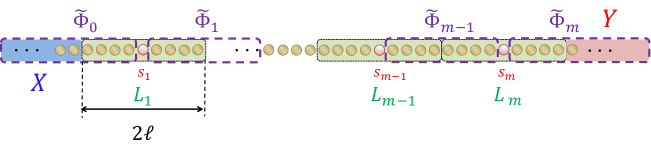
Figure 5: Approximating $\{\Phi_{j}\}_{j=0}^{m+1}$ by $\{\tilde{\Phi}_{j}\}_{j=0}^{m+1}$, the dependence on $h_{s_{1}},\ldots,h_{s_{m}}$ are removed from $\{\tilde{\Phi}_{j}\}_{j=0}^{m+1}$. These approximations allow a simple analysis to remove the zeroth-order terms for $h_{s_{1}},\ldots,h_{s_{m}}$.

We approximate each of $\{\Phi_{j}\}_{j=0}^{m+1}$ by $\{\tilde{\Phi}_{j}\}_{j=0}^{m+1}$ so that they do not include interaction terms $\{h_{s_{j}}\}_{j=1}^{m}$, respectively (see also Fig. 5). More precisely, $\tilde{\Phi}_{0}$, $\{\tilde{\Phi}_{j}\}_{j=1}^{m}$ and $\tilde{\Phi}_{m+1}$ are defined by using the subset Hamiltonians $H_{(-\infty,s_{1}]}$, $H_{(s_{j},s_{j+1}]}$ and $H_{(s_{m},\infty)}$, respectively. The approximation errors are given by

$$\left\|\Phi_{j}-\tilde{\Phi}_{j}\right\|\leq\mathcal{G}_{\beta}(\ell),$$ (141)

where the form of $\mathcal{G}_{\beta}(\ell)$ is given by Eq. (80). Using the above bound, we can derive the following lemma:

Lemma 13.

By defining $\Phi_{0:m}$ and $\tilde{\Phi}_{0:m}$ as

$$\Phi_{0:m}:=\Phi_{0}\Phi_{1}\cdots\Phi_{m},\quad\tilde{\Phi}_{0:m}:=\tilde{\Phi}_{0}\tilde{\Phi}_{1}\cdots\tilde{\Phi}_{m},$$ (142)

we obtain the following upper bound

$$\left\|\Phi_{0:m}-\tilde{\Phi}_{0:m}\right\|\leq(m+1)e^{m\tilde{g}\beta}\mathcal{G}_{\beta}(\ell)\leq 2me^{m\tilde{g}\beta}\mathcal{G}_{\beta}(\ell).$$ (143)

Proof of Lemma 13. For the proof, we define

$$\Phi_{0:m}^{(s)}:=\tilde{\Phi}_{0}\cdots\tilde{\Phi}_{s-1}\Phi_{s}\cdots\Phi_{m},$$ (144)

which yields

$$\Phi_{0:m}-\tilde{\Phi}_{0:m}=\sum_{s=0}^{m}\left(\Phi_{0:m}^{(s)}-\Phi_{0:m}^{(s+1)}\right),$$ (145)

where we use $\Phi_{0:m}^{(0)}=\Phi_{0:m}$ and $\Phi_{0:m}^{(m+1)}=\tilde{\Phi}_{0:m}$. From the definition and the upper bound (141), we have

$$\left\|\Phi_{0:m}^{(s)}-\Phi_{0:m}^{(s+1)}\right\| =\left\|\tilde{\Phi}_{0}\cdots\tilde{\Phi}_{s-1}\left(\Phi_{s}-\tilde{\Phi}_{s}\right)\Phi_{s+1}\cdots\Phi_{m}\right\|$$

$$\leq\left\|\tilde{\Phi}_{0}\right\|\cdots\left\|\tilde{\Phi}_{s}\right\|\cdot\mathcal{G}_{\beta}(\ell)\cdot\left\|\Phi_{s+1}\right\|\cdots\left\|\Phi_{m}\right\|\leq e^{m\tilde{g}\beta}\mathcal{G}_{\beta}(\ell),$$ (146)

where we use the upper bounds of

$$\left\|\Phi_{j}\right\|\leq e^{\beta\left\|h_{s_{j}}\right\|}\leq e^{\beta\tilde{g}},$$ (147)

Note that the same inequality holds for $\left\|\tilde{\Phi}_{j}\right\|$. By applying the inequality (V.2) to Eq. (145), we prove the main inequality (143). This completes the proof. $\square$

By denoting $H_{L_{0}}+H_{L_{1}}+\cdots+H_{L_{m+1}}$ by $H_{0}$, we have

$$\left\|e^{\beta H}-\tilde{\Phi}_{0:m}e^{\beta H_{0}}\tilde{\Phi}_{0:m}^{\dagger}\right\|_{1} =\left\|e^{\beta H}-\tilde{\Phi}_{0:m}\Phi_{0:m}^{-1}e^{\beta H}\left(\Phi_{0:m}^{\dagger}\right)^{-1}\tilde{\Phi}_{0:m}^{\dagger}\right\|_{1}$$

$$=\left\|\left(1-\tilde{\Phi}_{0:m}\Phi_{0:m}^{-1}\right)e^{\beta H}+\tilde{\Phi}_{0:m}\Phi_{0:m}^{-1}e^{\beta H}\left[1-\left(\Phi_{0:m}^{\dagger}\right)^{-1}\tilde{\Phi}_{0:m}^{\dagger}\right]\right\|_{1}$$

$$\leq\left(1+\left\|\tilde{\Phi}_{0:m}\Phi_{0:m}^{-1}\right\|\right)\left\|1-\tilde{\Phi}_{0:m}\Phi_{0:m}^{-1}\right\|\cdot\left\|e^{\beta H}\right\|_{1}$$

$$\leq(1+\left\|\tilde{\Phi}_{0:m}\right\|\cdot\left\|\Phi_{0:m}^{-1}\right\|)\left\|\Phi_{0:m}^{-1}\right\|\cdot\left\|\Phi_{0:m}-\tilde{\Phi}_{0:m}\right\|{\rm tr}\left(e^{\beta H}\right)$$

$$\leq 4me^{4(m+1)\beta\tilde{g}}\mathcal{G}_{\beta}(\ell){\rm tr}\left(e^{\beta H}\right),$$ (148)

where we use $\left\|\tilde{\Phi}_{0:m}\right\|\leq e^{(m+1)\beta\tilde{g}}$ and $\left\|\Phi_{0:m}^{-1}\right\|\leq e^{(m+1)\beta\tilde{g}}$. Therefore, under the definition of

$$\tilde{G}_{s_{1},s_{2},\ldots,s_{m}}:=\mathcal{D}_{h_{s_{1}},\ldots,h_{s_{m}}}\tilde{\Phi}_{0:m}e^{\beta H_{L_{0}}}e^{\beta H_{L_{1}}}\cdots e^{\beta H_{L_{m+1}}}\tilde{\Phi}_{0:m}^{\dagger},$$ (149)

we obtain from the inequality (136)

$${\rm Cor}_{\rho_{\beta}}(O_{X},O_{Y})\leq e^{m\Theta(\beta)}\mathcal{G}_{\beta}(\ell)+\frac{1}{Z_{\beta}}{\rm tr}\left(\Psi_{X,Y}\tilde{G}_{s_{1},s_{2},\ldots,s_{m}}\right),$$ (150)

where we use the error bound (V.2) to let $\epsilon\to e^{m\Theta(\beta)}\mathcal{G}_{\beta}(\ell)$ in (136).

Because $\tilde{\Phi}_{0:m}$ does not include the interaction terms $h_{s_{1}},\ldots,h_{s_{m}}$ and Hamiltonians $\{H_{L_{j}}\}_{j=0}^{m+1}$ commute with each other, we reduce Eq. (149) to

$$\tilde{G}_{s_{1},s_{2},\ldots,s_{m}}=\tilde{\Phi}_{0:m}e^{\beta H_{L_{0}}}\prod_{j=1}^{m}\left[e^{\beta H_{L_{j}}}-e^{\beta\left(H_{L_{j}}-h_{s_{j}}\right)}\right]e^{\beta H_{L_{m+1}}}\tilde{\Phi}_{0:m}^{\dagger}.$$ (151)

Therefore, we proceed to estimate an upper bound on

$${\rm tr}\left(\Psi_{X,Y}\tilde{G}_{s_{1},s_{2},\ldots,s_{m}}\right) ={\rm tr}\left(\Psi_{X,Y}\tilde{\Phi}_{0:m}e^{\beta H_{L_{0}}}\prod_{j=1}^{m}\left[e^{\beta H_{L_{j}}}-e^{\beta\left(H_{L_{j}}-h_{s_{j}}\right)}\right]e^{\beta H_{L_{m+1}}}\tilde{\Phi}_{0:m}\right).$$ (152)

We prove the following key subtheorem, which will be proved in the subsequent section VI.

Subtheorem 1.

The quantity $\left|{\rm tr}\left(\Psi_{X,Y}\tilde{G}_{s_{1},s_{2},\ldots,s_{m}}\right)\right|$ obeys the following the upper bound:

$$\left|{\rm tr}\left(\Psi_{X,Y}\tilde{G}_{s_{1},s_{2},\ldots,s_{m}}\right)\right|\leq \left[6e^{-me^{-\Theta(\beta)}}+e^{\Theta(m\beta)}\mathcal{G}_{\beta}(\ell)\right]{\rm tr}\left(e^{\beta H}\right).$$ (153)

V.3 Completing the proof

We now have all the ingredients to prove the main theorem. First, we have adopted the interaction-truncated Hamiltonian with interaction length $l_{0}$, which implies

$${\rm Cor}_{\rho_{\beta}}(O_{X},O_{Y})\leq{\rm Cor}_{\rho_{{\rm t},\beta}}(O_{X},O_{Y})+\Theta(1)\beta Rl_{0}\bar{J}(l_{0}),$$ (154)

where we use the inequality (III.2). Second, the inequality (150) with Subtheorem 1 gives

$${\rm Cor}_{\rho_{{\rm t},\beta}}(O_{X},O_{Y})\leq e^{m\Theta(\beta)}\mathcal{G}_{\beta}(\ell)+\left[6e^{-me^{-\Theta(\beta)}}+e^{\Theta(m\beta)}\mathcal{G}_{\beta}(\ell)\right].$$ (155)

By combining the above inequalities together, we arrive at the inequality of

$${\rm Cor}_{\rho_{\beta}}(O_{X},O_{Y})\leq e^{m\Theta(\beta)}\min\left(e^{-\ell/\Theta(\beta l_{0})},\left[\bar{J}(\ell/3)\right]^{1/\Theta(\beta)}\right)+\Theta(1)e^{-me^{-\Theta(\beta)}}+\Theta(1)\beta Rl_{0}\bar{J}(l_{0}),$$ (156)

where we use Eq. (80) for $\mathcal{G}_{\beta}(\ell)$.

We, in the following, denote the free parameters $\ell$ and $l_{0}$ as follows:

$$\ell=\frac{R}{c(R)},\quad m\propto\frac{R}{\ell}=c(R),\quad l_{0}=\frac{R}{c_{0}(R)},$$ (157)

where $c(R)$ and $c_{0}(R)$ are functions of $R$ and satisfy $c(R)<c_{0}(R)$ from the condition (139). We then reduce the inequality (156) to

$${\rm Cor}_{\rho_{\beta}}(O_{X},O_{Y})$$

$$\leq e^{\Theta(\beta)c(R)}\min\left[e^{-\frac{c_{0}(R)}{\Theta(\beta)c(R)}},\bar{J}\left(\frac{R}{3c(R)}\right)^{1/\Theta(\beta)}\right]+\Theta(1)e^{-c(R)e^{-\Theta(\beta)}}+\frac{\Theta(1)\beta R^{2}}{c_{0}(R)}\bar{J}\left(\frac{R}{c_{0}(R)}\right),$$ (158)

The remaining task is to appropriately choose $c_{0}(R)$ and $c(R)$ to attain the desired inequalities (17) and (1) for the sub-exponential decay of the interactions and the other interaction forms, respectively.

We first consider the sub-exponential decay of the interactions, i.e.,

$$\bar{J}(r)\leq e^{-\Theta(r^{\kappa})}.$$ (159)

In this case, we adopt

$$c(R)=\Theta(1)c_{0}(R),$$ (160)

and

$$\min\left[e^{-\frac{c_{0}(R)}{\Theta(\beta)c(R)}},\bar{J}\left(\frac{R}{3c(R)}\right)\right]^{1/\Theta(\beta)}\leq\bar{J}\left(\frac{R}{3c(R)}\right)^{1/\Theta(\beta)}\leq\exp\left[-\frac{1}{\Theta(\beta)}\left(\frac{R}{c(R)}\right)^{\kappa}\right].$$ (161)

Then, we impose the following condition for the first term in the RHS of (156):

$$e^{\Theta(\beta)c(R)}\exp\left[-\frac{1}{\Theta(\beta)}\left(\frac{R}{c(R)}\right)^{\kappa}\right]\leq\exp\left[-\frac{1}{2\Theta(\beta)}\left(\frac{R}{c(R)}\right)^{\kappa}\right],$$ (162)

which is satisfied by choosing

$$c(R)=\Theta(1)\frac{R^{\kappa/(\kappa+1)}}{\beta^{2/(\kappa+1)}}.$$ (163)

Under the above choices of $c_{0}(R)$ and $c(R)$, we obtain

$${\rm Cor}_{\rho_{\beta}}(O_{X},O_{Y})\leq\Theta(1)e^{-R^{\kappa/(\kappa+1)}/e^{\Theta(\beta)}},$$ (164)

which reduces to the first main inequality (17).

We second consider the slower decay than the sub-exponential decay, i.e.,

$$\lim_{r\to\infty}e^{-r^{\kappa}}/\bar{J}(r)=0\quad\textrm{for}\quad\forall\kappa>0.$$ (165)

In that case, we adopt

$$\min\left[e^{-\frac{c_{0}(R)}{\Theta(\beta)c(R)}},\bar{J}\left(\frac{R}{3c(R)}\right)\right]^{1/\Theta(\beta)}\leq\exp\left[-\frac{c_{0}(R)}{\Theta(\beta)c(R)}\right].$$ (166)

We impose the condition of

$$e^{\Theta(\beta)c(R)}\exp\left[-\frac{c_{0}(R)}{\Theta(\beta)c(R)}\right]\leq\exp\left[-\frac{c_{0}(R)}{2\Theta(\beta)c(R)}\right]$$

$$\longrightarrow c(R)=\frac{\sqrt{c_{0}(R)}}{\Theta(\beta)},$$ (167)

in a way similar to (162).

Finally, we choose the function $c(R)$ such that

$$e^{-c(R)e^{-\Theta(\beta)}}\leq\bar{J}(R)\longrightarrow c(R)=e^{\Theta(\beta)}\log\left[\bar{J}(R)^{-1}\right],\quad c_{0}(R)=e^{\Theta(\beta)}\log^{2}\left[\bar{J}(R)^{-1}\right],$$ (168)

where we use $c_{0}(R)=\Theta(\beta^{2})c(R)^{2}=e^{\Theta(\beta)}\log^{2}\left[\bar{J}(R)^{-1}\right]$. Under the above choices of $c_{0}(R)$ and $c(R)$, we reduce the inequality (156) to

$${\rm Cor}_{\rho_{\beta}}(O_{X},O_{Y})\leq\left(\frac{R}{e^{\Theta(\beta)}}\right)^{2}\bar{J}\left(\frac{R}{e^{\Theta(\beta)}\log^{2}\left[\bar{J}(R)^{-1}\right]}\right),$$ (169)

which gives the second main inequality (1). This completes the proof of Theorem 1. $\square$

VI Proof of Subtheorem 1

We first explicitly write the target quantity $\tilde{G}_{s_{1},s_{2},\ldots,s_{m}}$ in Eq. (151) as follows:

$$\tilde{G}_{s_{1},s_{2},\ldots,s_{m}}=\tilde{\Phi}_{0:m}e^{\beta H_{L_{0}}}\prod_{j=1}^{m}\left(e^{\beta H_{L_{j}}}-e^{\beta(H_{L_{j}}-h_{s_{j}})}\right)e^{\beta H_{L_{m+1}}}\tilde{\Phi}_{0:m}^{\dagger}$$

$$=\tilde{\Phi}_{0:m}e^{\beta H_{L_{0}}}\prod_{j=1}^{m}\left(e^{\beta H_{L_{j}}(\lambda_{j}=1)}-e^{\beta H_{L_{j}}(\lambda_{j}=0)}\right)e^{\beta H_{L_{m+1}}}\tilde{\Phi}_{0:m}^{\dagger}$$

$$=(-1)^{m}\sum_{\vec{\lambda}=\{0,1\}^{\otimes m}}(-1)^{\lambda_{1}+\lambda_{2}+\cdots+\lambda_{m}}\tilde{\Phi}_{0:m}\exp\left(\beta\sum_{j=0}^{m+1}H_{L_{j}}(\lambda_{j})\right)\tilde{\Phi}_{0:m}^{\dagger},$$ (170)

where we parametrize the interaction term $h_{s_{j}}$ by $\lambda_{j}h_{s_{j}}$ and denote the Hamiltonian $H_{L_{j}}(\lambda_{j})=H_{L_{j}}-(1-\lambda_{j})h_{s_{j}}$; for $j=0,m+1$, we fix $\lambda_{0}=\lambda_{m+1}=1$ and set $H_{L_{0}}(\lambda_{0}=1)=H_{L_{0}}$ and $H_{L_{m+1}}(\lambda_{m+1}=1)=H_{L_{m+1}}$.

As has been defined in Sec. V.2, each of the approximate belief propagation operators $\{\tilde{\Phi}_{j}\}_{j=0}^{m+1}$ are defined so that they do not include interaction terms $\{h_{s_{j}}\}_{j=1}^{m}$, respectively (Fig. 5). Hence, using Lemma 13 [or the inequality (V.2)], for an arbitrary set of $\vec{\lambda}$, we have

$$\left\|\tilde{\Phi}_{0:m}\exp\left(\beta\sum_{j=0}^{m+1}H_{L_{j}}(\lambda_{j})\right)\tilde{\Phi}_{0:m}^{\dagger}-e^{\beta H(\vec{\lambda})}\right\| \leq e^{\Theta(m\beta)}\mathcal{G}_{\beta}(\ell){\rm tr}\left(e^{\beta H(\vec{\lambda})}\right),$$ (171)

where $H(\vec{\lambda})$ is the parametrization Hamiltonian as follows:

$$H(\vec{\lambda})=H-\sum_{j=1}^{m}(1-\lambda_{j})h_{s_{j}}.$$ (172)

Note that the Golden-Thompson inequality provides

$${\rm tr}\left(e^{\beta H(\vec{\lambda})}\right)\leq{\rm tr}\left(e^{\beta H}e^{-\beta\sum_{j=1}^{m}(1-\lambda_{j})h_{s_{j}}}\right) \leq{\rm tr}\left(e^{\beta H}e^{\beta\sum_{j=1}^{m}(1-\lambda_{j})\left\|h_{s_{j}}\right\|}\right)$$

$$\leq e^{\beta m\tilde{g}}{\rm tr}\left(e^{\beta H}\right),$$ (173)

where we use $\left\|h_{s_{j}}\right\|\leq\tilde{g}$ from (52). By applying the inequalities (171) and (VI) to Eq. (VI), we have

$$\left\|\tilde{G}_{s_{1},s_{2},\ldots,s_{m}}-(-1)^{m}\sum_{\vec{\lambda}=\{0,1\}^{\otimes m}}(-1)^{\lambda_{1}+\lambda_{2}+\cdots+\lambda_{m}}e^{\beta H(\vec{\lambda})}\right\|_{1}$$

$$\leq 2^{m}e^{\Theta(m\beta)}\mathcal{G}_{\beta}(\ell){\rm tr}\left(e^{\beta H}\right)\leq e^{\Theta(m\beta)}\mathcal{G}_{\beta}(\ell){\rm tr}\left(e^{\beta H}\right),$$ (174)

which also implies

$$\left|{\rm tr}\left(\Psi_{X,Y}\tilde{G}_{s_{1},s_{2},\ldots,s_{m}}\right)\right|\leq\left|{\rm tr}\left(\Psi_{X,Y}(-1)^{m}\sum_{\vec{\lambda}=\{0,1\}^{\otimes m}}(-1)^{\lambda_{1}+\lambda_{2}+\cdots+\lambda_{m}}e^{\beta H(\vec{\lambda})}\right)\right|+e^{\Theta(m\beta)}\mathcal{G}_{\beta}(\ell){\rm tr}\left(e^{\beta H}\right),$$ (175)

where we use $\left\|\Psi_{X,Y}\right\|\leq 2$.

In the following, we consider the operator of

$$\Gamma:=(-1)^{m}\sum_{\vec{\lambda}=\{0,1\}^{\otimes m}}(-1)^{\lambda_{1}+\lambda_{2}+\cdots+\lambda_{m}}e^{\beta H(\vec{\lambda})},$$ (176)

which makes the inequality (175)

$$\left|{\rm tr}\left(\Psi_{X,Y}\tilde{G}_{s_{1},s_{2},\ldots,s_{m}}\right)\right|\leq\left|{\rm tr}\left(\Psi_{X,Y}\Gamma\right)\right|+e^{\Theta(m\beta)}\mathcal{G}_{\beta}(\ell){\rm tr}\left(e^{\beta H}\right).$$ (177)

For this purpose we define $H_{\geq j_{0}}(\vec{\lambda})$ as

$$H_{\geq j_{0}}(\vec{\lambda}_{\geq j_{0}})=H_{0}+\sum_{j=j_{0}}^{m}\lambda_{j}h_{s_{j}},\quad H_{0}:=H(\vec{0}),\quad H_{\geq 1}(\vec{\lambda})=H_{1:q}(\vec{\lambda}),$$ (178)

where we define $\vec{\lambda}_{\geq j_{0}}=\{\lambda_{j}\}_{j=j_{0}}^{m}$. We then define the belief propagation operator $\Phi_{s_{1}}(\vec{\lambda}_{\geq 1})$ as

$$e^{\beta H(\vec{\lambda})}=\Phi_{s_{1}}(\vec{\lambda}_{\geq 1})e^{\beta\left(H(\vec{\lambda})-\lambda_{1}h_{s_{1}}\right)}\Phi_{s_{1}}(\vec{\lambda}_{\geq 1})^{\dagger}=\Phi_{s_{1}}(\vec{\lambda}_{\geq 1})e^{\beta H_{\geq 2}(\vec{\lambda}_{\geq 2})}\Phi_{s_{1}}(\vec{\lambda}_{\geq 1})^{\dagger},$$ (179)

where $\Phi_{s_{1}}(\vec{\lambda}_{\geq 1})$ is trivially given by the identity operator for $\lambda_{1}=0$:

$$\Phi_{s_{1}}(\vec{\lambda}_{\geq 1})=\hat{1}\quad\textrm{for}\quad\lambda_{1}=0.$$ (180)

We next define $\Phi_{s_{2}}(\vec{\lambda}_{\geq 2})$ as the belief propagation operator of

$$e^{\beta H_{\geq 2}(\vec{\lambda}_{\geq 2})}=\Phi_{s_{2}}(\vec{\lambda}_{\geq 2})e^{\beta\left(H_{\geq 2}(\vec{\lambda}_{\geq 2})-\lambda_{2}h_{s_{2}}\right)}\Phi_{s_{2}}(\vec{\lambda}_{\geq 2})=\Phi_{s_{2}}(\vec{\lambda}_{\geq 2})e^{\beta\left(H_{\geq 3}(\vec{\lambda}_{\geq 3})\right)}\Phi_{s_{2}}(\vec{\lambda}_{\geq 2}),$$ (181)

In the same way, we define $\Phi_{s_{j}}(\vec{\lambda}_{\geq j})$ as the belief propagation operator of

$$e^{\beta H_{\geq j}(\vec{\lambda}_{\geq j})}=\Phi_{s_{j}}(\vec{\lambda}_{\geq j})e^{\beta H_{\geq j+1}(\vec{\lambda}_{\geq j+1})}\Phi_{s_{j}}(\vec{\lambda}_{\geq j}),\quad\Phi_{s_{j}}(\vec{\lambda}_{\geq j})=\hat{1}\quad\textrm{for}\quad\lambda_{j}=0.$$ (182)

where the Hamiltonian $H_{\geq j+1}(\vec{\lambda}_{\geq j+1})$ includes the interaction terms $h_{s_{j+1}},h_{s_{j+2}},\ldots,h_{s_{q}}$. By using the above operators, we have

$$e^{\beta H(\vec{\lambda})}= \Phi_{s_{1}}(\vec{\lambda}_{\geq 1})\Phi_{s_{2}}(\vec{\lambda}_{\geq 2})\cdots\Phi_{s_{m}}(\vec{\lambda}_{\geq m})e^{\beta H(\vec{0})}\left[\Phi_{s_{1}}(\vec{\lambda}_{\geq 1})\Phi_{s_{2}}(\vec{\lambda}_{\geq 2})\cdots\Phi_{s_{m}}(\vec{\lambda}_{\geq m})\right]^{\dagger}.$$ (183)

For the belief propagation operator in Eq. (182), we can construct the approximate version $\Phi_{s_{j}}(\lambda_{j})$ so that it is constructed from the Hamiltonian $H_{L_{j}}$, where $s_{j}$ was defined as the center site in the region $L_{j}$ (see Fig. 5). Then, the approximation error is obtained from (80) as follows:

$$\left\|\Phi_{s_{j}}(\vec{\lambda}_{\geq j})-\tilde{\Phi}_{s_{j},L_{j}}(\lambda_{j})\right\|\leq\mathcal{G}_{\beta}(\ell),$$ (184)

where we use the fact that $L_{j}$ has the width of $2\ell$. Note that $H_{L_{j}}$ only includes the interaction term $h_{s_{j}}$, and hence the operator $\tilde{\Phi}_{s_{j},L_{j}}(\vec{\lambda}_{\geq j})$ depends only on $\lambda_{j}$. By combining the above upper bound with Lemma 13, we obtain

$$\left\|e^{\beta H(\vec{\lambda})}-\tilde{\Phi}_{s_{1},L_{1}}(\lambda_{1})\tilde{\Phi}_{s_{2},L_{2}}(\lambda_{2})\cdots\tilde{\Phi}_{s_{m},L_{m}}(\lambda_{m})e^{\beta H(\vec{0})}\left[\tilde{\Phi}_{s_{1},L_{1}}(\lambda_{1})\tilde{\Phi}_{s_{2},L_{2}}(\lambda_{2})\cdots\tilde{\Phi}_{s_{m},L_{m}}(\lambda_{m})\right]^{\dagger}\right\|_{1}$$

$$\leq e^{\Theta(m\beta)}\mathcal{G}_{\beta}(\ell){\rm tr}\left(e^{\beta H(\vec{\lambda})}\right)\leq e^{\Theta(m\beta)}\mathcal{G}_{\beta}(\ell){\rm tr}\left(e^{\beta H}\right),$$ (185)

where we use the relation (VI) in the last inequality. Therefore, by defining $\tilde{\Gamma}$ as

$$\tilde{\Gamma}:=(-1)^{m}\sum_{\vec{\lambda}=\{0,1\}^{\otimes m}}(-1)^{\lambda_{1}+\lambda_{2}+\cdots+\lambda_{m}}\tilde{\Phi}_{s_{1},L_{1}}(\lambda_{1})\cdots\tilde{\Phi}_{s_{m},L_{m}}(\lambda_{m})e^{\beta H(\vec{0})}\left[\tilde{\Phi}_{s_{1},L_{1}}(\lambda_{1})\cdots\tilde{\Phi}_{s_{m},L_{m}}(\lambda_{m})\right]^{\dagger},$$ (186)

by analogy to Eq. (176), we can obtain from (VI)

$$\left\|\Gamma-\tilde{\Gamma}\right\|_{1}\leq e^{\Theta(m\beta)}\mathcal{G}_{\beta}(\ell){\rm tr}\left(e^{\beta H}\right),$$ (187)

where we use an inequality similar to (174). By combining the above inequality with the upper bound (177), we obtain

$$\left|{\rm tr}\left(\Psi_{X,Y}\tilde{G}_{s_{1},s_{2},\ldots,s_{m}}\right)\right|\leq \left|{\rm tr}\left(\Psi_{X,Y}\tilde{\Gamma}\right)\right|+e^{\Theta(m\beta)}\mathcal{G}_{\beta}(\ell){\rm tr}\left(e^{\beta H}\right).$$ (188)

The final task is to estimate $\left|{\rm tr}\left(\Psi_{X,Y}\tilde{\Gamma}\right)\right|$.

We first notice that $\tilde{\Phi}_{s_{j},L_{j}}(\lambda_{j})$ is an approximate belief propagation operator supported on $L_{j}$. Hence, we can ensure $[\tilde{\Phi}_{s_{j},L_{j}}(\lambda_{j}),\tilde{\Phi}_{s_{j^{\prime}},L_{j^{\prime}}}(\lambda_{j^{\prime}})]=0$ as well as $[\tilde{\Phi}_{s_{j},L_{j}}(\lambda_{j}),\Psi_{X,Y}]=0$. We remind that we have chosen as $L_{0}=X$ and $L_{m+1}=Y$. We therefore obtain a similar decomposition to the classical case (119):

$${\rm tr}\left(\Psi_{X,Y}\tilde{\Gamma}\right)$$

$$=(-1)^{m}\sum_{\vec{\lambda}=\{0,1\}^{\otimes m}}(-1)^{\lambda_{1}+\lambda_{2}+\cdots+\lambda_{m}}{\rm tr}\left(\Psi_{X,Y}\tilde{\Phi}_{s_{1},L_{1}}(\lambda_{1})\cdots\tilde{\Phi}_{s_{m},L_{m}}(\lambda_{m})e^{\beta H(\vec{0})}\left[\tilde{\Phi}_{s_{1},L_{1}}(\lambda_{1})\cdots\tilde{\Phi}_{s_{m},L_{m}}(\lambda_{m})\right]^{\dagger}\right)$$

$$={\rm tr}\left[\Psi_{X,Y}\prod_{j=1}^{m}\left(\tilde{\Phi}_{s_{j},L_{j}}^{\dagger}\tilde{\Phi}_{s_{j},L_{j}}-1\right)e^{\beta H(\vec{0})}\right]$$

$$={\rm tr}\left[(\Psi_{X,Y}+2)^{1/2}\prod_{j=1}^{m}\left(\tilde{\Phi}_{s_{j},L_{j}}^{\dagger}\tilde{\Phi}_{s_{j},L_{j}}-1\right)e^{\beta H(\vec{0})}(\Psi_{X,Y}+2)^{1/2}\right]-2{\rm tr}\left[\prod_{j=1}^{m}\left(\tilde{\Phi}_{s_{j},L_{j}}^{\dagger}\tilde{\Phi}_{s_{j},L_{j}}-1\right)e^{\beta H(\vec{0})}\right],$$ (189)

where we use $\tilde{\Phi}_{s_{j},L_{j}}(0)=\hat{1}$ and denote $\tilde{\Phi}_{s_{j},L_{j}}(1)=\tilde{\Phi}_{s_{j},L_{j}}$ for simplicity, and the last inequality is simply derived by $(\Psi_{X,Y}+2)^{1/2}(\Psi_{X,Y}+2)^{1/2}-2=\Psi_{X,Y}$. Note that $\Psi_{X,Y}+2$ is positive semidefinite because of $\left\|\Psi_{X,Y}\right\|\leq 2$. To compute $\left|{\rm tr}\left(\Psi_{X,Y}\tilde{\Gamma}\right)\right|$, we generally consider

$${\rm tr}\left(O_{X,Y}{\rm tr}_{L_{1:m}}\left[\prod_{j=1}^{m}\left(\tilde{\Phi}_{s_{j},L_{j}}^{\dagger}\tilde{\Phi}_{s_{j},L_{j}}-1\right)e^{\beta H(\vec{0})}\right]O_{X,Y}\right),$$ (190)

where $O_{X,Y}$ is an arbitrary positive semidefinite Hermitian operator supported on $XY$. For this purpose, we calculate

$$\Bra{\tilde{\psi}_{X,Y}}{\rm tr}_{L_{1:m}}\left[\prod_{j=1}^{m}\left(\tilde{\Phi}_{s_{j},L_{j}}^{\dagger}\tilde{\Phi}_{s_{j},L_{j}}-1\right)e^{\beta H(\vec{0})}\right]\Ket{\tilde{\psi}_{X,Y}},$$ (191)

with

$$\ket{\tilde{\psi}_{X,Y}}:=O_{X,Y}\ket{\psi_{X,Y}},$$ (192)

where $\ket{\psi_{X,Y}}$ is an arbitrary quantum state supported on the subset $XY$. We then prove the following lemma which is useful in evaluating Eq. (191).

Lemma 14.

Let $\{W_{j}\}_{j=1}^{m}$ be arbitrary semi-definite operators (i.e., $W_{j}\succeq 0$) supported on $X\subset\Lambda$ and commute with each other. We then obtain

$$\bra{\psi_{X^{\rm c}}}{\rm tr}_{X}\left(\rho\prod_{j=1}^{m}W_{j}\right)\ket{\psi_{X^{\rm c}}}\leq\bra{\psi_{X^{\rm c}}}{\rm tr}_{X}\left[\rho\prod_{j=1}^{m}(W_{j}+1)\right]\ket{\psi_{X^{\rm c}}}\cdot\prod_{j=1}^{m}\frac{\left\|W_{j}\right\|}{\left\|W_{j}\right\|+1},$$ (193)

where $\rho$ is an arbitrary positive semi-definite operator as $\rho\succeq 0$.

Proof. We first define the notations of

$$\rho_{X}=\bra{\psi_{X^{\rm c}}}\rho\ket{\psi_{X^{\rm c}}},\quad W_{j}=\sum_{x}w_{j,x}\ket{x}\bra{x},$$ (194)

where the latter one is the spectral decomposition of $W_{j}$ using the simultaneous eigenstates $\{\ket{x}\}_{x}$ of $\{W_{j}\}_{j=1}^{m}$. Note that we have assumed $[W_{j},W_{j^{\prime}}]=0$ for an arbitrary pair of $j,j^{\prime}$. Because $\{W_{j}\}_{j=1}^{m}$ are positive semi-definite, we can ensure $w_{j,x}\geq 0$ for $\forall j,x$. Therefore, we have the following equation:

$$\bra{\psi_{X^{\rm c}}}{\rm tr}_{X}\left(\rho\prod_{j=1}^{m}W_{j}\right)\ket{\psi_{X^{\rm c}}}={\rm tr}_{X}\left(\rho_{X}\prod_{j=1}^{m}W_{j}\right)=\sum_{x}\bra{x}\rho_{X}\ket{x}\prod_{j=1}^{m}w_{j,x}.$$ (195)

In the same way, we have

$$\bra{\psi_{X^{\rm c}}}{\rm tr}_{X}\left[\rho\prod_{j=1}^{m}(W_{j}+1)\right]\ket{\psi_{X^{\rm c}}}=\sum_{x}\bra{x}\rho_{X}\ket{x}\prod_{j=1}^{m}\left(w_{j,x}+1\right).$$ (196)

By letting $\bra{x}\rho_{X}\ket{x}=\rho_{x}$, we have

$$\bra{\psi_{X^{\rm c}}}{\rm tr}_{X}\left(\rho\prod_{j=1}^{m}W_{j}\right)\ket{\psi_{X^{\rm c}}}=\bra{\psi_{X^{\rm c}}}{\rm tr}_{X}\left[\rho\prod_{j=1}^{m}(W_{j}+1)\right]\ket{\psi_{X^{\rm c}}}\frac{\sum_{x}\rho_{x}\prod_{j=1}^{m}w_{j,x}}{\sum_{x}\rho_{x}\prod_{j=1}^{m}\left(w_{j,x}+1\right)}.$$ (197)

In the following, we define

$$\tilde{W}_{j_{0}}:=\sum_{x}\rho_{x}\prod_{j=1}^{j_{0}}\left(w_{j,x}+1\right)\prod_{j=j_{0}+1}^{m}w_{j,x},$$ (198)

where $\tilde{W}_{0}=\sum_{x}\rho_{x}\prod_{j=1}^{m}w_{j,x}$ and $\tilde{W}_{m}=\sum_{x}\rho_{x}\prod_{j=1}^{m}(w_{j,x}+1)$. We then consider

$$\frac{\sum_{x}\rho_{x}\prod_{j=1}^{m}w_{j,x}}{\sum_{x}\rho_{x}\prod_{j=1}^{m}\left(w_{j,x}+1\right)}=\frac{\tilde{W}_{0}}{\tilde{W}_{m}}=\frac{\tilde{W}_{0}}{\tilde{W}_{1}}\cdot\frac{\tilde{W}_{1}}{\tilde{W}_{2}}\cdot\frac{\tilde{W}_{2}}{\tilde{W}_{3}}\cdots\frac{\tilde{W}_{m-1}}{\tilde{W}_{m}}.$$ (199)

For an arbitrary $j_{0}\in[1,m]$, we have

$$\frac{\tilde{W}_{j_{0}-1}}{\tilde{W}_{j_{0}}} =\frac{\sum_{x}\rho_{x}\prod_{j=1}^{j_{0}-1}\left(w_{j,x}+1\right)w_{j_{0},x}\prod_{j=j_{0}+1}^{m}w_{j,x}}{\sum_{x}\rho_{x}\prod_{j=1}^{j_{0}-1}\left(w_{j,x}+1\right)(w_{j_{0},x}+1)\prod_{j=j_{0}+1}^{m}w_{j,x}}$$

$$=\frac{\sum_{x}\rho_{x}w_{j_{0},x}Q_{j_{0},x}}{\sum_{x}\rho_{x}(w_{j_{0},x}+1)Q_{j_{0},x}},\quad Q_{j_{0},x}:=\prod_{j=1}^{j_{0}-1}\left(w_{j,x}+1\right)\prod_{j=j_{0}+1}^{m}w_{j,x}.$$ (200)

We then obtain the following inequality for the derivatives of

$$\frac{d}{d_{w_{j_{0},x}}}\frac{\sum_{x}\rho_{x}w_{j_{0},x}Q_{j_{0},x}}{\sum_{x}\rho_{x}(w_{j_{0},x}+1)Q_{j_{0},x}} =\frac{\rho_{x}Q_{j_{0},x}}{\sum_{x}\rho_{x}(w_{j_{0},x}+1)Q_{j_{0},x}}-\frac{\sum_{x}\rho_{x}w_{j_{0},x}Q_{j_{0},x}}{\sum_{x}\rho_{x}(w_{j_{0},x}+1)Q_{j_{0},x}}\cdot\frac{\rho_{x}Q_{j_{0},x}}{\sum_{x}\rho_{x}(w_{j_{0},x}+1)Q_{j_{0},x}}$$

$$=\frac{\rho_{x}Q_{j_{0},x}}{\sum_{x}\rho_{x}(w_{j_{0},x}+1)Q_{j_{0},x}}\left(1-\frac{\sum_{x}\rho_{x}w_{j_{0},x}Q_{j_{0},x}}{\sum_{x}\rho_{x}(w_{j_{0},x}+1)Q_{j_{0},x}}\right)\geq 0,$$ (201)

where we use the positivities of $\{w_{j,x}\}_{j,x}$, which also implies $Q_{j_{0},x}\geq 0$. Because of $w_{j_{0},x}\leq\left\|W_{j_{0}}\right\|$, we can drive the inequality of

$$\frac{\tilde{W}_{j_{0}-1}}{\tilde{W}_{j_{0}}}\leq\frac{\sum_{x}\rho_{x}\left\|W_{j_{0}}\right\|Q_{j_{0},x}}{\sum_{x}\rho_{x}(\left\|W_{j_{0}}\right\|+1)Q_{j_{0},x}}=\frac{\left\|W_{j_{0}}\right\|}{\left\|W_{j_{0}}\right\|+1}.$$ (202)

By applying the above upper bound to Eq. (199), we prove the desired inequality (193). This completes the proof. $\square$

We apply Lemma 14 to Eq. (191) with

$$X\to L_{1:m},\quad\ket{\psi_{X}}\to\frac{\ket{\tilde{\psi}_{X,Y}}}{\left\|O_{X,Y}\ket{\psi_{X,Y}}\right\|},\quad W_{j}\to\tilde{\Phi}_{s_{j},L_{j}}^{\dagger}\tilde{\Phi}_{s_{j},L_{j}}-1.$$ (203)

Then, we obtain

$$\Bra{\tilde{\psi}_{X,Y}}{\rm tr}_{L_{1:m}}\left[\prod_{j=1}^{m}\left(\tilde{\Phi}_{s_{j},L_{j}}^{\dagger}\tilde{\Phi}_{s_{j},L_{j}}-1\right)e^{\beta H(\vec{0})}\right]\Ket{\tilde{\psi}_{X,Y}}$$

$$=\left\|O_{X,Y}\ket{\psi_{X,Y}}\right\|^{2}\frac{\Bra{\tilde{\psi}_{X,Y}}}{\left\|O_{X,Y}\ket{\psi_{X,Y}}\right\|}{\rm tr}_{L_{1:m}}\left[\prod_{j=1}^{m}\left(\tilde{\Phi}_{s_{j},L_{j}}^{\dagger}\tilde{\Phi}_{s_{j},L_{j}}-1\right)e^{\beta H(\vec{0})}\right]\frac{\Ket{\tilde{\psi}_{X,Y}}}{\left\|O_{X,Y}\ket{\psi_{X,Y}}\right\|}$$

$$\leq\Bra{\tilde{\psi}_{X,Y}}{\rm tr}_{L_{1:m}}\left[\prod_{j=1}^{m}\tilde{\Phi}_{s_{j},L_{j}}^{\dagger}\tilde{\Phi}_{s_{j},L_{j}}e^{\beta H(\vec{0})}\right]\Ket{\tilde{\psi}_{X,Y}}\cdot\prod_{j=1}^{m}\frac{\left\|\tilde{\Phi}_{s_{j},L_{j}}^{\dagger}\tilde{\Phi}_{s_{j},L_{j}}\right\|-1}{\left\|\tilde{\Phi}_{s_{j},L_{j}}^{\dagger}\tilde{\Phi}_{s_{j},L_{j}}\right\|}$$

$$=\Bra{\psi_{X,Y}}O_{X,Y}{\rm tr}_{L_{1:m}}\left[\tilde{\Phi}_{s_{1},L_{1}}\cdots\tilde{\Phi}_{s_{m},L_{m}}e^{\beta H(\vec{0})}\left(\tilde{\Phi}_{s_{1},L_{1}}\cdots\tilde{\Phi}_{s_{m},L_{m}}\right)^{\dagger}\right]O_{X,Y}\Ket{\psi_{X,Y}}\prod_{j=1}^{m}\frac{\left\|\tilde{\Phi}_{s_{j},L_{j}}^{\dagger}\tilde{\Phi}_{s_{j},L_{j}}\right\|-1}{\left\|\tilde{\Phi}_{s_{j},L_{j}}^{\dagger}\tilde{\Phi}_{s_{j},L_{j}}\right\|}.$$ (204)

We recall that it has been denoted $\tilde{\Phi}_{s_{j},L_{j}}(1)=\tilde{\Phi}_{s_{j},L_{j}}$ in (189). We here denote the spectral decomposition of the Hilbert space on the subset $X,Y$ by

$$\hat{1}_{X,Y}:=\sum_{x}\Ket{x_{X,Y}}\Bra{x_{X,Y}}.$$ (205)

By applying the upper bound (204) to Eq. (190), we have

$${\rm tr}\left(O_{X,Y}\left[\prod_{j=1}^{m}\left(\tilde{\Phi}_{s_{j},L_{j}}^{\dagger}\tilde{\Phi}_{s_{j},L_{j}}-1\right)e^{\beta H(\vec{0})}\right]O_{X,Y}\right)=\sum_{x}\Bra{x_{X,Y}}O_{X,Y}\prod_{j=1}^{m}\left(\tilde{\Phi}_{s_{j},L_{j}}^{\dagger}\tilde{\Phi}_{s_{j},L_{j}}-1\right)e^{\beta H(\vec{0})}O_{X,Y}\Ket{x_{X,Y}}$$

$$\leq\prod_{j=1}^{m}\frac{\left\|\tilde{\Phi}_{s_{j},L_{j}}^{\dagger}\tilde{\Phi}_{s_{j},L_{j}}\right\|-1}{\left\|\tilde{\Phi}_{s_{j},L_{j}}^{\dagger}\tilde{\Phi}_{s_{j},L_{j}}\right\|}\sum_{x}\Bra{x_{X,Y}}O_{X,Y}{\rm tr}_{L_{1:m}}\left[\tilde{\Phi}_{s_{1},L_{1}}\cdots\tilde{\Phi}_{s_{m},L_{m}}e^{\beta H(\vec{0})}\left(\tilde{\Phi}_{s_{1},L_{1}}\cdots\tilde{\Phi}_{s_{m},L_{m}}\right)^{\dagger}\right]O_{X,Y}\Ket{x_{X,Y}}$$

$$\leq\prod_{j=1}^{m}\frac{\left\|\tilde{\Phi}_{s_{j},L_{j}}^{\dagger}\tilde{\Phi}_{s_{j},L_{j}}\right\|-1}{\left\|\tilde{\Phi}_{s_{j},L_{j}}^{\dagger}\tilde{\Phi}_{s_{j},L_{j}}\right\|}{\rm tr}\left[O_{X,Y}\tilde{\Phi}_{s_{1},L_{1}}\cdots\tilde{\Phi}_{s_{m},L_{m}}e^{\beta H(\vec{0})}\left(\tilde{\Phi}_{s_{1},L_{1}}\cdots\tilde{\Phi}_{s_{m},L_{m}}\right)^{\dagger}O_{X,Y}\right]$$

$$\leq\prod_{j=1}^{m}\frac{\left\|\tilde{\Phi}_{s_{j},L_{j}}^{\dagger}\tilde{\Phi}_{s_{j},L_{j}}\right\|-1}{\left\|\tilde{\Phi}_{s_{j},L_{j}}^{\dagger}\tilde{\Phi}_{s_{j},L_{j}}\right\|}\left[{\rm tr}\left(O_{X,Y}e^{\beta H}O_{X,Y}\right)+\left\|O_{X,Y}\right\|^{2}e^{\Theta(m\beta)}\mathcal{G}_{\beta}(\ell){\rm tr}\left(e^{\beta H}\right)\right]$$

$$\leq\left\|O_{X,Y}\right\|^{2}\left[1+e^{\Theta(m\beta)}\mathcal{G}_{\beta}(\ell)\right]{\rm tr}\left(e^{\beta H}\right)\prod_{j=1}^{m}\frac{\left\|\tilde{\Phi}_{s_{j},L_{j}}^{\dagger}\tilde{\Phi}_{s_{j},L_{j}}\right\|-1}{\left\|\tilde{\Phi}_{s_{j},L_{j}}^{\dagger}\tilde{\Phi}_{s_{j},L_{j}}\right\|},$$ (206)

where we use the inequality (VI) in the third inequality. By applying this inequality to $\left|{\rm tr}\left(\Psi_{X,Y}\tilde{\Gamma}\right)\right|$ in Eq. (189), we can derive

$$\left|{\rm tr}\left(\Psi_{X,Y}\tilde{\Gamma}\right)\right|\leq\left(\left\|\Psi_{X,Y}\right\|+4\right)\left[1+e^{\Theta(m\beta)}\mathcal{G}_{\beta}(\ell)\right]{\rm tr}\left(e^{\beta H}\right)\prod_{j=1}^{m}\frac{\left\|\tilde{\Phi}_{s_{j},L_{j}}^{\dagger}\tilde{\Phi}_{s_{j},L_{j}}\right\|-1}{\left\|\tilde{\Phi}_{s_{j},L_{j}}^{\dagger}\tilde{\Phi}_{s_{j},L_{j}}\right\|}.$$ (207)

Finally, from the inequality (147), we have

$$\left\|\tilde{\Phi}_{s_{j},L_{j}}^{\dagger}\tilde{\Phi}_{s_{j},L_{j}}\right\|\leq e^{\Theta(\beta)},$$ (208)

and hence we obtain

$$\prod_{j=1}^{m}\frac{\left\|\tilde{\Phi}_{s_{j},L_{j}}^{\dagger}\tilde{\Phi}_{s_{j},L_{j}}\right\|-1}{\left\|\tilde{\Phi}_{s_{j},L_{j}}^{\dagger}\tilde{\Phi}_{s_{j},L_{j}}\right\|}\leq\prod_{j=1}^{m}\left(1-e^{-\Theta(\beta)}\right)\leq e^{-me^{-\Theta(\beta)}},$$ (209)

where we use $(1+x)^{m}\leq e^{mx}$ for arbitrary real $x$ with $|x|\leq 1$ and $m\in\mathbb{N}^{+}$. We thus arrived at the inequality of

$$\left|{\rm tr}\left(\tilde{\Gamma}\right)\right|\leq 6\left[1+e^{\Theta(m\beta)}\mathcal{G}_{\beta}(\ell)\right]e^{-me^{-\Theta(\beta)}}{\rm tr}\left(e^{\beta H}\right),$$ (210)

where we use $\left\|\Psi_{X,Y}\right\|\leq 2$. By combining the inequalities (210) and (188), we prove the main inequality (153). This completes the proof. $\square$

VII Concluding remarks

In this paper, we have demonstrated a clustering theorem that applies to systems beyond those with finite-range or exponentially decaying interactions. The core findings and significant observations are encapsulated in Theorem 1. Our methodology integrates the quantum belief propagation technique, combined with a specific decomposition approach outlined in Section V.2. This approach enables us to replicate analyses typical of classical one-dimensional systems, effectively circumventing the cluster expansion divergence (see Section IV.1). Our findings conclusively address several aspects of the clustering theorem within one-dimensional quantum systems: i) the dependence of correlation length on temperature, ii) the behavior of correlation decay rates for interactions decaying slower than subexponential forms.

Despite these advancements, our study unveils several unresolved issues. Among the most critical is improving the correlation decay rate in one-dimensional systems with subexponential (or faster) interaction decay. This challenge primarily stems from the approximation used in the inequality (V.2). To minimize the error in the approximate belief propagation, i.e., $\mathcal{G}_{\beta}(\ell)$, a larger block size $\ell$ is necessary. Yet, this results in fewer blocks ($m\propto R/\ell$), leading to a less strict decay rate of $e^{-m/e^{\Theta(\beta)}}$ as per equation (153). At this stage, the improvement is not a straightforward task, and addressing this issue may require fundamentally novel analytical methods.

One potential strategy for overcoming this challenge involves analyzing the zero-free region of the partition function, as discussed in [27]. This entails to find a complex number $z$ such that the partition function satisfies

$$Z_{\beta+iz}={\rm tr}\left(e^{(\beta+iz)H}\right)\neq 0$$

for any $|z|\leq\Delta$, with $\Delta>0$. By proving a zero-free region for the partition function for $\Delta=\Omega(1)$, we can prove the exponential clustering theorem from [27, Theorem 10 therein]. Achieving this would leverage a bootstrapping method: initially applying the current ‘loose’ clustering theorem to establish the zero-free region, then applying this result to refine the clustering of correlation based on Ref. [27]. This approach is anticipated to be viable if the quasi-locality $\mathcal{G}_{\beta}(r)$ decays exponentially with distance $r$, applicable in scenarios of interactions decaying (faster than) exponentially.

Furthermore, analyzing the complex zeros of the partition function reveals additional implications. The current clustering theorem does not exclude the possibility of a phase transition in systems with power-law decaying interaction, since the correlation decay is polynomial in both critical and non-critical phases. A zero-free region for $|z|\leq\Delta=\Omega(1)$ leads to the partition function’s analyticity in the thermodynamic limit, suggesting the absence of phase transition in long-range interacting systems. So far, there are no quantum analogs to the classical no-go theorem [13] for the phase transition in long-range interacting systems. We speculate that the critical condition for the power-law decay rate $\alpha$ might also be $2$ in quantum scenarios, yet this remains a significant open question. We hope that our new analytical techniques including the quantum belief propagation will pave the way for resolving further open questions regarding the 1D long-range interacting systems.

VIII Acknowledgements

Y. K. and T. K. acknowledge the Hakubi projects of RIKEN. T. K. was supported by the Japan Science and Technology Agency Precursory Research for Embryonic Science and Technology (Grant No. JPMJPR2116). We are grateful to Nikhil Srivastava for helpful discussions and comments on related topics.

References

- Ising et al. [2017] T. Ising, R. Folk, R. Kenna, B. Berche, and Y. Holovatch, The Fate of Ernst Ising and the Fate of his Model (2017), arXiv:1706.01764 [physics.hist-ph] .
- Araki [1969] H. Araki, Gibbs states of a one dimensional quantum lattice, Communications in Mathematical Physics 14, 120 (1969).
- Dobrushin and Shlosman [1987] R. L. Dobrushin and S. B. Shlosman, Completely analytical interactions: Constructive description, Journal of Statistical Physics 46, 983 (1987).
- Kubo [1957] R. Kubo, Statistical-Mechanical Theory of Irreversible Processes. I. General Theory and Simple Applications to Magnetic and Conduction Problems, Journal of the Physical Society of Japan 12, 570 (1957).
- Martin and Schwinger [1959] P. C. Martin and J. Schwinger, Theory of Many-Particle Systems. I, Phys. Rev. 115, 1342 (1959).
- Araki [1978] H. Araki, On the Kubo-Martin-Schwinger Boundary Condition, Progress of Theoretical Physics Supplement 64, 12 (1978), https://academic.oup.com/ptps/article-pdf/doi/10.1143/PTPS.64.12/5288493/64-12.pdf .
- Onsager [1944] L. Onsager, Crystal Statistics. I. A Two-Dimensional Model with an Order-Disorder Transition, Phys. Rev. 65, 117 (1944).
- Stanley [1971] H. E. Stanley, Phase transitions and critical phenomena, Vol. 7 (Clarendon Press, Oxford, 1971).
- Dyson [1969] F. J. Dyson, Existence of a phase-transition in a one-dimensional Ising ferromagnet, Communications in Mathematical Physics 12, 91 (1969).
- Fisher et al. [1972] M. E. Fisher, S.-k. Ma, and B. G. Nickel, Critical Exponents for Long-Range Interactions, Phys. Rev. Lett. 29, 917 (1972).
- Kosterlitz [1976] J. M. Kosterlitz, Phase Transitions in Long-Range Ferromagnetic Chains, Phys. Rev. Lett. 37, 1577 (1976).
- Thouless [1969] D. J. Thouless, Long-Range Order in One-Dimensional Ising Systems, Phys. Rev. 187, 732 (1969).
- Dobrushin [1973] R. L. Dobrushin, Analyticity of correlation functions in one-dimensional classical systems with slowly decreasing potentials, Communications in Mathematical Physics 32, 269 (1973).
- Kuwahara and Saito [2020a] T. Kuwahara and K. Saito, Area law of noncritical ground states in 1D long-range interacting systems, Nature Communications 11, 4478 (2020a).
- Araki [1975] H. Araki, On uniqueness of KMS states of one-dimensional quantum lattice systems, Communications in Mathematical Physics 44, 1 (1975).
- Kishimoto [1976] A. Kishimoto, On uniqueness of KMS states of one-dimensional quantum lattice systems, Communications in Mathematical Physics 47, 167 (1976).
- Pérez-García and Pérez-Hernández [2023] D. Pérez-García and A. Pérez-Hernández, Locality Estimates for Complex Time Evolution in 1D, Communications in Mathematical Physics 399, 929 (2023).
- Bouch [2015] G. Bouch, Complex-time singularity and locality estimates for quantum lattice systems, Journal of Mathematical Physics 56, 123303 (2015), https://pubs.aip.org/aip/jmp/article-pdf/doi/10.1063/1.4936209/13525869/123303_1_online.pdf .
- Kuwahara and Saito [2018] T. Kuwahara and K. Saito, Polynomial-time Classical Simulation for One-dimensional Quantum Gibbs States, arXiv preprint arXiv:1807.08424 (2018), arXiv:1807.08424 .
- Bluhm et al. [2022] A. Bluhm, Á. Capel, and A. Pérez-Hernández, Exponential decay of mutual information for Gibbs states of local Hamiltonians, Quantum 6, 650 (2022).
- Kato and Brandão [2019] K. Kato and F. G. S. L. Brandão, Quantum Approximate Markov Chains are Thermal, Communications in Mathematical Physics 10.1007/s00220-019-03485-6 (2019).
- Bardet et al. [2023] I. Bardet, A. Capel, L. Gao, A. Lucia, D. Pérez-García, and C. Rouzé, Rapid Thermalization of Spin Chain Commuting Hamiltonians, Phys. Rev. Lett. 130, 060401 (2023).
- Brandao and Cramer [2015] F. G. S. L. Brandao and M. Cramer, Equivalence of Statistical Mechanical Ensembles for Non-Critical Quantum Systems (2015), arXiv:1502.03263 [quant-ph] .
- Kuwahara and Saito [2020b] T. Kuwahara and K. Saito, Eigenstate Thermalization from the Clustering Property of Correlation, Phys. Rev. Lett. 124, 200604 (2020b).
- Kuwahara and Saito [2020c] T. Kuwahara and K. Saito, Gaussian concentration bound and Ensemble equivalence in generic quantum many-body systems including long-range interactions, Annals of Physics 421, 168278 (2020c).
- Fawzi et al. [2023] H. Fawzi, O. Fawzi, and S. O. Scalet, A subpolynomial-time algorithm for the free energy of one-dimensional quantum systems in the thermodynamic limit, Quantum 7, 1011 (2023).
- Harrow et al. [2020] A. W. Harrow, S. Mehraban, and M. Soleimanifar, Classical Algorithms, Correlation Decay, and Complex Zeros of Partition Functions of Quantum Many-Body Systems, in Proceedings of the 52nd Annual ACM SIGACT Symposium on Theory of Computing, pages = 378–386, numpages = 9, series = STOC 2020 (Association for Computing Machinery, New York, NY, USA, 2020).
- Hastings [2007] M. B. Hastings, Quantum belief propagation: An algorithm for thermal quantum systems, Phys. Rev. B 76, 201102 (2007).
- Kim [2012] I. H. Kim, Perturbative analysis of topological entanglement entropy from conditional independence, Phys. Rev. B 86, 245116 (2012).
- Lieb and Robinson [1972] E. Lieb and D. Robinson, The finite group velocity of quantum spin systems, Communications in Mathematical Physics 28, 251 (1972).
- Bravyi et al. [2006] S. Bravyi, M. B. Hastings, and F. Verstraete, Lieb-Robinson Bounds and the Generation of Correlations and Topological Quantum Order, Phys. Rev. Lett. 97, 050401 (2006).
- Brandão and Kastoryano [2019] F. G. S. L. Brandão and M. J. Kastoryano, Finite Correlation Length Implies Efficient Preparation of Quantum Thermal States, Communications in Mathematical Physics 365, 1 (2019).
- Anshu et al. [2021] A. Anshu, S. Arunachalam, T. Kuwahara, and M. Soleimanifar, Sample-efficient learning of interacting quantum systems, Nature Physics 17, 931 (2021).
- Kuwahara et al. [2021] T. Kuwahara, A. M. Alhambra, and A. Anshu, Improved Thermal Area Law and Quasilinear Time Algorithm for Quantum Gibbs States, Phys. Rev. X 11, 011047 (2021).
- Kuwahara and Saito [2022] T. Kuwahara and K. Saito, Exponential clustering of bipartite quantum entanglement at arbitrary temperatures, Phys. Rev. X 12, 021022 (2022).
- Gross [1979] L. Gross, Decay of correlations in classical lattice models at high temperature, Communications in Mathematical Physics 68, 9 (1979).
- Park and Yoo [1995] Y. M. Park and H. J. Yoo, Uniqueness and clustering properties of Gibbs states for classical and quantum unbounded spin systems, Journal of Statistical Physics 80, 223 (1995).
- Ueltschi [2004] D. Ueltschi, Cluster expansions and correlation functions, Moscow Mathematical Journal 4, 511 (2004).
- Kliesch et al. [2014] M. Kliesch, C. Gogolin, M. J. Kastoryano, A. Riera, and J. Eisert, Locality of Temperature, Phys. Rev. X 4, 031019 (2014).
- Fröhlich and Ueltschi [2015] J. Fröhlich and D. Ueltschi, Some properties of correlations of quantum lattice systems in thermal equilibrium, Journal of Mathematical Physics 56, 053302 (2015).
- Kuwahara et al. [2020] T. Kuwahara, K. Kato, and F. G. S. L. Brandão, Clustering of Conditional Mutual Information for Quantum Gibbs States above a Threshold Temperature, Phys. Rev. Lett. 124, 220601 (2020).
- [42] D. Kim, T. Kuwahara, and K. Saito, In preparation, .
- Kotecký and Preiss [1986] R. Kotecký and D. Preiss, Cluster expansion for abstract polymer models, Communications in Mathematical Physics 103, 491 (1986).
- Mann and Minko [2024] R. L. Mann and R. M. Minko, Algorithmic Cluster Expansions for Quantum Problems, PRX Quantum 5, 010305 (2024).
- Hastings and Koma [2006] M. Hastings and T. Koma, Spectral Gap and Exponential Decay of Correlations, Communications in Mathematical Physics 265, 781 (2006).
- Nachtergaele et al. [2006] B. Nachtergaele, Y. Ogata, and R. Sims, Propagation of Correlations in Quantum Lattice Systems, Journal of Statistical Physics 124, 1 (2006).
- Nachtergaele and Sims [2006] B. Nachtergaele and R. Sims, Lieb-Robinson Bounds and the Exponential Clustering Theorem, Communications in Mathematical Physics 265, 119 (2006).
- Kuwahara [2015] T. Kuwahara, Fundamental inequalities in quantum many-body systems, PhD thesis, University of Tokyo (2015).
- Kuwahara and Saito [2021] T. Kuwahara and K. Saito, Lieb-Robinson Bound and Almost-Linear Light Cone in Interacting Boson Systems, Phys. Rev. Lett. 127, 070403 (2021).