Long-range Ising model for regional-scale seismic risk analysis

Abstract

This study introduces the long-range Ising model from statistical mechanics to the Performance-Based Earthquake Engineering (PBEE) framework for regional seismic damage analysis. The application of the PBEE framework at a regional scale entails estimating the damage states of numerous structures, typically performed using fragility function-based stochastic simulations. However, these simulations often assume independence or employ simplistic dependency models among capacities of structures, leading to significant misrepresentation of risk. The Ising model addresses this issue by converting the available information on binary damage states (safe or failure) into a joint probability mass function, leveraging the principle of maximum entropy. The Ising model offers two main benefits: (1) it requires only the first- and second-order cross-moments, enabling seamless integration with the existing PBEE framework, and (2) it provides meaningful physical interpretations of the model parameters, facilitating the uncovering of insights not apparent from data. To demonstrate the proposed method, we applied the Ising model to $156$ buildings in Antakya, Turkey, using post-hazard damage evaluation data, and to $182$ buildings in Pacific Heights, San Francisco, using simulated data from the Regional Resilience Determination (R2D) tool. In both instances, the Ising model accurately reproduces the provided information and generates meaningful insights into regional damages. The study also investigates the change in Ising model parameters under varying earthquake magnitudes, along with the mean-field approximation, further facilitating the applicability of the proposed approach.

1 Introduction

The Performance-Based Earthquake Engineering (PBEE) framework has been extensively developed and utilized for over 20 years, providing a systematic method to calculate quantifiable metrics for seismic design and post-hazard decision-making [1, 2]. To incorporate the various uncertainties that propagate from ground motions to the seismic performance of a structure, the PBEE framework considers four groups of random variables: (1) ground motion intensity measure (IM), (2) engineering demand parameter (EDP), (3) damage measure or damage state (DS), and (4) loss or decision variable (DV), each described by its probability distribution. Given an earthquake scenario, IM is typically described as a probability distribution $P(IM)$, or as a mean annual probability of exceedance $\lambda(IM)$, assuming a Poisson process model for the temporal occurrence of earthquakes. This intensity measure model is followed by the conditional distribution of EDP given IM, denoted by $P(EDP|IM)$. Subsequently, the conditional distribution of DS given EDP, $P(DS|EDP)$, is established, which can also be expressed as a complementary cumulative distribution function, or component-level fragility function, $G(DS|EDP)$. Finally, $G(DS|EDP)$ is followed by the distribution of DV given DS, $P(DV|DS)$. To obtain the exceedance probability $\lambda(DV)$ of a decision variable, the probability density functions $P(\cdot)$ are often transformed to complementary cumulative distribution functions $G(\cdot)$, yielding the integral:

$$\lambda(DV)=\int_{DS}\int_{EDP}\int_{IM}G(DV|DS)d\,G(DS|EDP)d\,G(EDP|IM)d\,\lambda(IM)\,.$$ (1)

Building on Eq. (1), the PBEE framework has been applied to a wide variety of structures, including braced steel frames [3], reinforced concrete moment-frame buildings [4, 5], and highway bridges [6]. These applications aim at individual structures, reflecting the original scope of the PBEE framework [7].

Recently, the application of the PBEE framework has been actively extended to a regional scale [7, 8, 9, 10]. In this context, Eq. (1) is typically solved using Monte Carlo methods that simulate regional responses to hazards, hereinafter referred to as regional seismic simulations. This simulation approach is favored because a system-level decision variable may depend on the damage states of all components, rendering Eq. (1) high-dimensional. Similar to the component-level applications, a regional-scale PBEE analysis can be decomposed into four modules: (1) IM generation, (2) EDP estimation, (3) DS evaluation, and (4) DV assessment. For each of these modules, physics-based or statistical methods/models can be employed, offering a spectrum of variations. For instance, to generate IM samples, one can simulate seismic wave propagation [11] to create synthetic seismograms or employ empirical ground motion prediction equations [12]. Nonlinear structural dynamic analysis can be performed to generate EDP samples [10], while several regression models directly connecting EDP to IM are also available [13, 14]. The DS can be obtained from structural analysis or inferred from IM or EDP samples using DS-IM or DS-EDP fragility curves. Lastly, DV can be assessed using loss curves that relate DS or EDP to DV [15], or physics-based simulations [9].

Physics-based simulations can accurately capture the complex interactions and correlations among structural responses and functionalities. However, they are often restricted to scenario-based analyses due to their extensive computational costs. On the other hand, statistical approaches, such as fragility function-based simulations of DS given EDP or IM [16], are computationally feasible but require many ad-hoc, sometimes subjective, assumptions about statistical models. Specifically, applying structural-level fragility functions to regional-scale analysis entails constructing a fragility field that summarizes the joint information across the region. To capture the spatial dependency among structural damages, the fragility field demands additional assumptions and parameters than individual fragility curves. The common practice of using individual fragility functions under the assumption of conditional independence (conditional on site-specific intensity measures) can significantly underestimate system-level failure probabilities [17].

This study presents an alternative method for constructing the fragility field, which can be integrated with fragility-based approaches, physics-based simulations, and even post-hazard survey data. Specifically, we introduce the Ising model, a widely recognized model in statistical mechanics, as a joint probability mass function for binary damage states (safe or failure) of structures over a region. Beyond its applications in statistical mechanics, the Ising model has been used across various disciplines to examine collective behaviors in complex systems, including DNA sequence reconstruction, ecological relationships, and financial markets [18]. This versatility stems from its nature as the maximum entropy distribution for binary variables, subject to constraints on first- and second-order cross-moments. Recently, maximum entropy distributions have been applied to regional seismic simulation of road networks [19], where the focus is on the computational aspects of maximum entropy modeling and the use of an efficient surrogate model. This study positions the Ising model within the PBEE framework, concentrating on the meaningful interpretation of model parameters and simulation results.

Section 2 overviews the current approaches for evaluating structural damages in the regional-scale PBEE. Subsequently, Section 3 introduces the formulation and parameter estimation of the Ising model in the context of regional seismic analysis. This section also develops the mean-field approximation to qualitatively explain the Ising model parameters. Section 4 offers interpretations of the Ising model parameters in the language of regional seismic risk analysis and explores their relationship with the mean and correlation coefficients of the damage states of structures. Section 5 demonstrates the validity and engineering relevance of the Ising model through two examples using real-world post-hazard survey data and synthetic simulation data, emphasizing the insights derived from the Ising model. Finally, concluding remarks and future research directions are presented in Section 6.

2 Current approaches for probabilistic structural damage predictions on a regional-scale

For an individual structure, the following fragility function is commonly used to predict its damage state:

$$\mathbb{P}\left(DS\geq ds_{i}|IM=im\right)=\Phi\left(\frac{\ln\left(im/\theta_{i}\right)}{\beta_{i}}\right)\,,$$ (2)

where $ds_{i}$ represents the $i$-th damage state, $IM$ denotes the ground motion intensity at the location of the structure, $\Phi(\cdot)$ is the standard Gaussian cumulative distribution function, $\theta_{i}$ is the median of $IM$ causing the damage $ds_{i}$ or greater, and $\beta_{i}$ denotes the log standard deviation of $IM$ that induces the damage $ds_{i}$ or greater. In regional seismic simulations, it is a common practice to construct fragility functions for each structure and assume conditional independence between the damage states of structures. Upon generating spatially correlated ground motion intensity measures, damage states of the structures are sampled according to Eq. (2) to produce a damage map [20, 16, 8, 21]. Subsequently, decision variables such as economic loss, casualties, increased traffic time, and welfare loss are calculated.

The missing information in the above procedure is the correlation between damage states contributed by the similarities of structures. Bazzurro and Luco Nicolas [22] emphasized that accounting for the similarity of structures represents a key distinction between analyzing a single structure and a portfolio of structures in the seismic loss estimation. Similarities between structures, such as the number of stories, construction materials, and structural type, are particularly pronounced in residential neighborhoods where structures share similar designs and are built following the same design codes. This contributes to the correlation between their damage states [17], in addition to the contribution from the spatial coherency of ground motions. To model the structure-to-structure damage correlation, Lee and Kiremidjian [23] presented a simplified approach by assuming equi-correlation among all structures. The study also concluded that the challenge of modeling the damage correlation lies in approximating the joint discrete damage distribution. Due to the difficulty of defining a joint distribution for discrete damage states, Baker and Cornell [24] proposed using the joint continuous distribution for the decision variables given the engineering demand parameters, $f(\boldsymbol{DV}|\boldsymbol{EDP})$, by integrating $f(\boldsymbol{DM}|\boldsymbol{EDP})$ and $f(\boldsymbol{DV}|\boldsymbol{DM})$, thereby bypassing the need for a joint distribution of discrete damage states. An alternative approach, as detailed in [25, 26], models fragility using continuous demand and capacity. This method has become popular because of its convenience.

The log-normal and other assumptions in fragility functions were largely motivated by convenience rather than by fundamental statistical and physical principles [27]. In the following sections, we will develop a joint distribution model for discrete damage states of structures that hinges on a single, fundamental assumption of statistical mechanics.

3 Long-range Ising model as a joint probability mass function for damage states

The Ising model was originally conceived as a mathematical model for ferromagnetism in statistical mechanics [28, 29]. A key feature of the model is that it represents the maximum entropy distribution constrained by the means and pairwise correlations, making it applicable to a wide variety of fields beyond statistical mechanics [30, 31, 18]. Provided with the first- and second-order cross-moments of the component states in a system, the Ising model is the least structured joint probability distribution for the component states that reproduces the prior information. In this section, we first formulate the Ising model within the context of regional seismic analysis, followed by a discussion on its parameter estimation. Finally, we present the mean-field approximation, which offers a qualitative understanding of the relationship between the Ising model parameters and the given statistics.

3.1 Formulation

Consider a region consisting of $n$ structures under an earthquake and assume that each structure can be in one of the binary states of safe or failure. Here, “safe” and “failure” are relative terms with respect to a target performance level. The group of structures has $N=2^{n}$ configurations, where the probability of the $I$-th configuration is expressed as:

$$P_{I}=\mathbb{P}\left(X_{1}=x_{1I},X_{2}=x_{2I},\dots,X_{n}=x_{nI}\right)\,,$$ (3)

where $X_{i}\in\{-1\text{ (safe)},1\text{ (failure)}\}$ is a random variable representing the state of the $i$-th structure, and $x_{iI}$ denotes an outcome of $X_{i}$ for the $I$-th configuration.

The entropy $S$ for $\boldsymbol{X}=[X_{1},X_{2},...,X_{n}]^{\intercal}$ is defined as

$$S\coloneqq-\sum_{I=1}^{N}P_{I}\log{P_{I}}.$$ (4)

In the absence of information, the probability distribution that maximizes the entropy is the uniform distribution, which means that all possible configurations are equally likely. Suppose we have information up to the second-order cross-moments expressed as follows:

$$\mathcal{M}_{1,i}=\sum_{I=1}^{N}x_{iI}P_{I}\,,$$ (5)

$$\mathcal{M}_{2,ij}=\sum_{I=1}^{N}x_{iI}x_{jI}P_{I}\,,i,j=1,2,...,n\,,$$ (6)

where $\mathcal{M}_{1,i}$ is the first-order cross-moment, i.e., the mean of $X_{i}$, and $\mathcal{M}_{2,ij}$ is the second-order cross-moment between the damage states of the $i$-th and $j$-th structures. Applying Lagrange multipliers with $\mathcal{M}_{1,i}$ and $\mathcal{M}_{2,ij}$ as constraints, the joint probability $P_{I}$ that maximizes the entropy $S$ is:

$$P_{I}=\frac{1}{Z}\exp{\left(\sum_{i=1}^{n}h_{i}x_{iI}+\sum_{i>j}J_{ij}x_{iI}x_{jI}\right)}\,,$$ (7)

where $Z$ is the normalizing constant given as:

$$Z=\sum_{I=1}^{N}\exp{\left(\sum_{i=1}^{n}h_{i}x_{iI}+\sum_{i>j}J_{ij}x_{iI}x_{jI}\right)}\,,$$ (8)

where $h_{i}$ and $J_{ij}$ are the Lagrange multiplies to meet the first- and second-order cross-moment constraints, respectively. The detailed derivation is presented in A. Since our goal is to model the joint distribution that outputs the probability for any specified configuration, we drop the subscript $I$ in Eq. (7) and replace $P_{I}$ by $p(\boldsymbol{x})$:

$$p(\boldsymbol{x}) =\frac{1}{Z}\exp{\left(\sum_{i=1}^{n}h_{i}x_{i}+\sum_{i>j}J_{ij}x_{i}x_{j}\right)}$$ (9)

$$=\frac{1}{Z}\exp{\left(\boldsymbol{h}\cdot\boldsymbol{x}+\frac{1}{2}\boldsymbol{x^{T}}\boldsymbol{J}\boldsymbol{x}\right)}\,,$$

where $\boldsymbol{x}=\left[x_{1},x_{2},\dots,x_{n}\right]^{\intercal}$, $\boldsymbol{h}=\left[h_{1},h_{2},\dots,h_{n}\right]^{\intercal}$, and

$$\boldsymbol{J}=\begin{bmatrix}0&J_{12}&\dots&J_{1n}\\ J_{12}&0&\dots&J_{2n}\\ \vdots&\vdots&\ddots&\vdots\\ J_{1n}&J_{2n}&\dots&0\end{bmatrix}\,.$$ (10)

Notice that Eq. (9) and Eq. (7) are equivalent, because any configuration of $\boldsymbol{x}$ is indexed by $I$. Eq. (9) is the Ising model for describing ferromagnetism, where $h_{i}$ and $J_{ij}$ can be interpreted as the external magnetic field acting on each component/spin and the pairwise coupling effects between each spin pair, respectively [28, 29]. While the classic Ising model features a sparse $\boldsymbol{J}$ because it considers only the pairwise interactions between neighboring spins on a lattice, Eq. (9) in this study represents a long-range or fully-connected Ising model, accounting for interactions between all pairs of structures in a region.

3.2 Parameter estimation

Parameter estimation of the Ising model, known as the inverse Ising problem, is challenging for large systems comprising numerous components. Existing computational techniques have yet to fully overcome the curse of dimensionality in solving inverse Ising problems involving over $10,000$ components [32, 33, 34, 35]. Nonetheless, for systems with hundreds of components, a variety of convex optimization algorithms are effective, owing to the convexity of the inverse Ising problem [18].

The Boltzmann machine learning, a widely used method for the inverse Ising problem, obtains the maximum likelihood estimation of the Ising model parameters through gradient-based optimization. The log-likelihood $\mathcal{L}$ of the parameters $\boldsymbol{h}$ and $\boldsymbol{J}$ given observations $\mathcal{D}=\{\boldsymbol{x}^{(1)},\boldsymbol{x}^{(2)},…,\boldsymbol{x}^{(M)}\}$ is given as:

$$\mathcal{L}(\boldsymbol{h},\boldsymbol{J}|\mathcal{D}) =\frac{1}{M}\ln{\left(\prod_{m=1}^{M}p(\boldsymbol{x}^{(m)}|\boldsymbol{h},\boldsymbol{J})\right)}$$ (11)

$$=\sum_{i=1}^{n}h_{i}\left(\frac{1}{M}\sum_{m=1}^{M}\sum_{i=1}^{n}x^{(m)}_{i}\right)+\sum_{i>j}J_{ij}\left(\frac{1}{M}\sum_{m=1}^{M}\sum_{i>j}x^{(m)}_{i}x^{(m)}_{j}\right)-\ln{Z(\boldsymbol{h},\boldsymbol{J})}$$

$$=\sum_{i=1}^{n}h_{i}\mathcal{M}_{1,i}^{\mathcal{D}}+\sum_{i>j}J_{ij}\mathcal{M}_{2,ij}^{\mathcal{D}}-\ln{Z(\boldsymbol{h},\boldsymbol{J})}\,,$$

where $\mathcal{M}_{1,i}^{\mathcal{D}}$ and $\mathcal{M}_{2,ij}^{\mathcal{D}}$ denote the first- and second-order cross-moments calculated from the observations $\mathcal{D}$. The final line of Eq. (11) reveals that the likelihood function hinges on $\mathcal{M}_{1,i}^{\mathcal{D}}$ and $\mathcal{M}_{2,ij}^{\mathcal{D}}$ rather than on the random samples in $\mathcal{D}$. This suggests that the Ising model can be applied when $\mathcal{M}_{1,i}^{\mathcal{D}}$ and $\mathcal{M}_{2,ij}^{\mathcal{D}}$ are derived from sources other than random samples. Consequently, the Ising model can be constructed using fragility functions [36, 37, 38], analytic models [39, 40, 41], or a combination of both [42], not requiring information beyond the current PBEE practice.

Notice that $\ln{Z}$ serves as a generating function for the first- and second-order cross-moments: $\frac{\partial\ln{Z}}{\partial h_{i}}=\mathcal{M}_{1,i}$ and $\frac{\partial\ln{Z}}{\partial J_{ij}}=\mathcal{M}_{2,ij}$. Using this property, differentiating Eq. (11) with respect to $h_{i}$ and $J_{ij}$ yields:

$$\frac{\partial\mathcal{L}}{\partial h_{i}}(\boldsymbol{h},\boldsymbol{J})=\mathcal{M}_{1,i}^{\mathcal{D}}-\mathcal{M}_{1,i}\,,$$ (12)

$$\frac{\partial\mathcal{L}}{\partial J_{ij}}(\boldsymbol{h},\boldsymbol{J})=\mathcal{M}_{2,ij}^{\mathcal{D}}-\mathcal{M}_{2,ij}\,.$$

Finally, we obtain the updating rule for the maximum likelihood estimation:

$$h_{i}^{(k+1)}=h_{i}^{(k)}+\alpha\frac{\partial\mathcal{L}}{\partial h_{i}}(\boldsymbol{h}^{(k)},\boldsymbol{J}^{(k)})=h_{i}^{(k)}+\alpha\left(\mathcal{M}_{1,i}^{\mathcal{D}}-\mathcal{M}_{1,i}\right)\,,$$ (13)

$$J_{ij}^{(k+1)}=J_{ij}^{(k)}+\alpha\frac{\partial\mathcal{L}}{\partial J_{ij}}(\boldsymbol{h}^{(k)},\boldsymbol{J}^{(k)})=J_{ij}^{(k)}+\alpha\left(\mathcal{M}_{2,ij}^{\mathcal{D}}-\mathcal{M}_{2,ij}\right)\,,$$

where $\alpha$ is the learning rate of the algorithm. Owing to the convexity of the inverse Ising problem, Eq .(13) is guaranteed to converge to a unique solution [18]. However, the exact evaluation of $\mathcal{M}_{1,i}$ and $\mathcal{M}_{2,ij}$ at each step requires calculating Eqs. (5) and (6) over $2^{n}$ configurations, which is generally infeasible. Hence, Monte Carlo sampling techniques are often used to approximate $\mathcal{M}_{1,i}$ and $\mathcal{M}_{2,ij}$ [43]. In this study, we adopted Gibbs sampling due to its applicability to high-dimensional distributions and ease of implementation.

3.3 Mean-field approximation

In this subsection, we introduce the mean-field approximation, one of the simplest approximation methods [44, 45, 18] for the inverse Ising problem, to facilitate the interpretation of the Ising model parameters. By averaging the interactions between components, the mean value of each component for a specified $\boldsymbol{h}$ and $\boldsymbol{J}$ is given by the solution of the following self-consistent equation:

$$m_{i}=\tanh\left({h_{i}+\sum_{j\neq i}J_{ij}m_{j}}\right)\,,$$ (14)

in which $m_{i}=\mathcal{M}_{1,i}$ denotes the mean value of the $i$-th component. The covariance can be obtained by solving:

$$c_{ij}=\left(1-m_{i}^{2}\right)\left(\delta_{ij}+\sum_{k\neq i}J_{ij}c_{kj}\right)\,,$$ (15)

where $c_{ij}$ is the covariance between the $i$-th and $j$-th components, which is equivalent to $\mathcal{M}_{2,ij}-\mathcal{M}_{1,i}\mathcal{M}_{1,j}$, and $\delta_{ij}$ is the Kronecker delta. The detailed derivation for the mean-field approximation is provided in B. Eqs. (14) and (15) represent the forward approximation that derives $m_{i}$ and $c_{ij}$ from the given $\boldsymbol{h}$ and $\boldsymbol{J}$. For the inverse Ising problem, the mean-field solution derived from the forward approximation is:

$$h_{i}=\tanh^{-1}{m_{i}}-\sum_{j\neq i}J_{ij}m_{j}\,,$$ (16)

$$J_{ij}=-\left(\boldsymbol{c}^{-1}\right)_{ij}\,,$$

where $\boldsymbol{c}$ is the covariance matrix with $c_{ij}$ as elements.

The accuracy and validity of the mean-field approximation depend on the magnitude and homogeneity of pairwise interactions, as the method averages these interactions and neglects individual effects [46]. Although various methods have been proposed to improve the applicability of the mean-field approximation, such as the Thouless-Anderson-Palmer (TAP) method [44, 18] and the Sessak-Monasson expansion [47], we found that none of these methods achieve satisfactory accuracy in regional seismic analysis. Therefore, our motivation of using the mean-field approximation is to facilitate a qualitative interpretation of the model parameters.

4 Parametric study of the Ising model

This section investigates the relationships between the Ising model parameters and typical performance quantities, such as failure probability and the correlation coefficient between damage states of structures, using simple proof-of-concept examples.

4.1 Interpretations of the Ising model parameters

• $\boldsymbol{h}$: We interpret $\boldsymbol{h}$ as a risk field acting on each structure within a region. According to Eq. (9), a structure with a positive $h_{i}$ is more probable to fail, i.e., to have a spin of $x_{i}=+1$, with a larger $h_{i}$ signifying a greater tendency towards failure. Conversely, a negative risk field $h_{i}$ indicates a tendency to remain safe. Given that civil structures are engineered to be reliable, they should inherently possess a negative field $-\mathcal{I}$, with $\mathcal{I}>0$. A hazard imposes an external positive field $h_{H}>0$ on each structure, and the resulting risk field is a balance between the hazard and the inertia towards remaining safe, i.e., $h_{i}=h_{H}-\mathcal{I}$. Here, both $h_{H}$ and $\mathcal{I}$ vary across structures.

• $\boldsymbol{J}$: This represents the pairwise interactions, reflecting the tendency of two structures to be in the same damage state. The term interaction encompasses all direct and indirect effects stemming from physical and statistical properties that determine how the damage state of one structure can affect the state of another. From Eq. (9), it is observed that if $J_{ij}$ is positive, the probability of two structures being in the same state is higher than them being in different states, with a larger $J_{ij}$ increasing this probability. On the other hand, a negative $J_{ij}$ favors the damage states being different.

The specific choice of terminology, such as risk field and pairwise interaction, can vary, but the fundamental implications of $\boldsymbol{h}$ and $\boldsymbol{J}$ remain invariant. Recall from Section 3 that the construction of the Ising model relies solely on the first- and second-order cross-moments. Therefore, it seems valid to claim that the Ising model cannot offer anything beyond the mean and the covariance matrix. However, it is important to acknowledge that the principle of maximum entropy introduces a crucial additional layer of information. Therefore, the Ising model encompasses more than just the mean and the covariance matrix.

4.2 Dependency between the Ising model parameters and the mean and correlation coefficient

Consider two binary random variables $\boldsymbol{X}=[X_{1},X_{2}]^{\intercal}\in\{-1\text{(safe)},1\text{(failure)}\}^{2}$ representing the damage states of two buildings. The risk field and pairwise interaction are given as $h_{1}=h_{2}=h$ and $J_{12}=J$, respectively. With only 2 variables and thus $2^{2}$ system configurations, the exact mean and correlation coefficient for given $h$ and $J$ values can be determined using Eqs. (5)-(9). The mean value $\mathbb{E}\left[X_{i}\right]$ is directly linked to the failure probability $P_{f}$ by $P_{f}=(\mathbb{E}\left[X_{i}\right]+1)/2$. Note that, due to parameter settings of the current demonstration, the failure probability $P_{f}$ for each building is the same.

The mean value for the damage state of a building is affected both by the risk field acting on the site and the pairwise interaction from the other building. Figure 1(a) depicts the mean damage state of a building with varying $h$ and $J$, and Figure 1(b) illustrates the relationship between the mean value and the risk field $h$ under four different $J$ values. The mean damage state of a building becomes larger as the risk field $h$ increases, reflecting that a stronger risk field results in a higher failure probability. Figure 1(b) also suggests that negative pairwise interaction provides a buffer for a building against the risk field. This is because to achieve the same mean damage $\mathbb{E}\left[X_{i}\right]>0$, negative $J$ requires larger $h$. In contrast, positive pairwise interaction increases a building’s sensitivity to the risk field, amplifying its tendency towards failure.

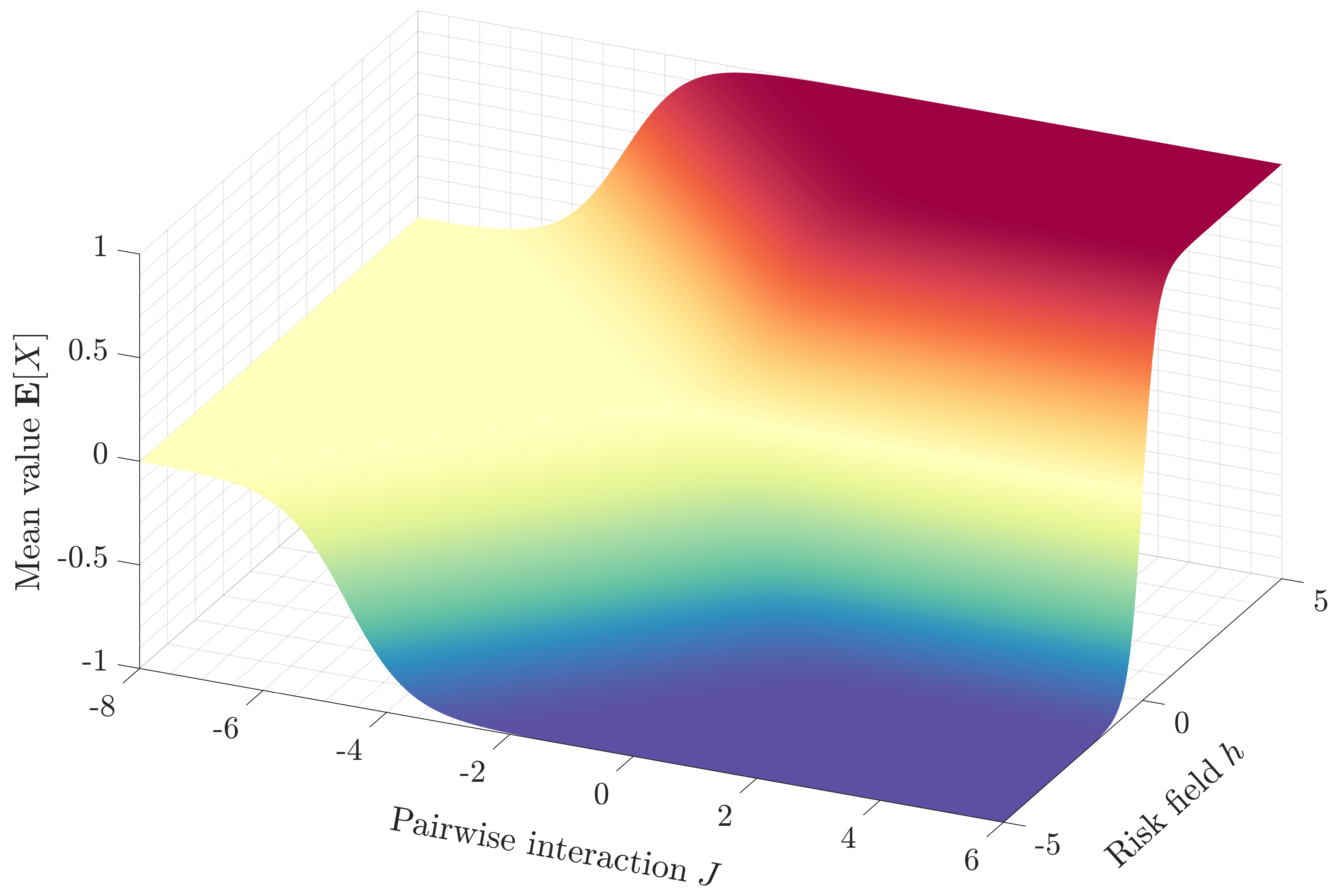
(a)

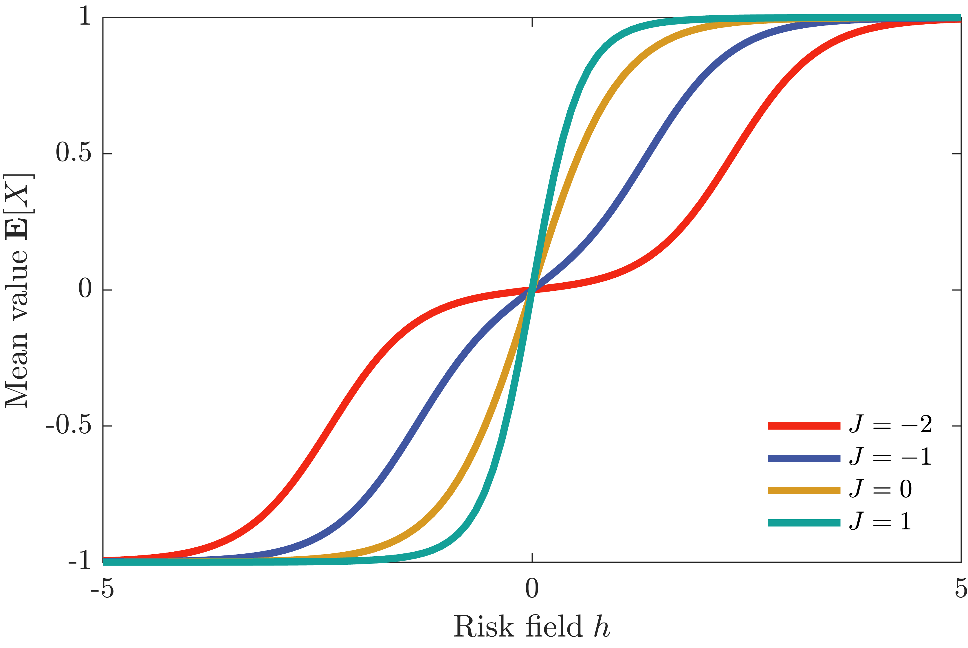
(b)

Figure 1: The relationship between the mean $\mathbb{E}\left[X_{i}\right]$, risk field $h$, and pairwise interaction $J$ for two buildings: (a) three-dimensional representation, and (b) two-dimensional illustration of $\mathbb{E}\left[X_{i}\right]$ against $h$ for four $J$ values. For any $J$, the mean damage state $\mathbb{E}\left[X_{i}\right]$ is monotonically increasing with respect to $h$. A negative interaction $J$ flattens the increase, while a positive $J$ steepens it.

Figures 2 reveals that the correlation coefficient of the damage states is influenced by both the pairwise interaction $J$ and the risk field $h$. For a given $h$, the correlation coefficient is monotonically increasing with respect to $J$. Increasing the absolute value of $h$ will make the $\rho$-$J$ dependency weaker. This occurs because, for large $|h|$, the joint distribution is dominated by the term $\sum_{i}h_{i}x_{i}$, rather than $\sum_{i>j}J_{ij}x_{i}x_{j}$, and the term $\sum_{i}h_{i}x_{i}$ implies independence. Moreover, the sign of $h$ will not influence the $\rho$-$J$ dependency for this simple model with two structures; this particular observation cannot be generalized to long-range Ising models with nonhomogeneous parameters.

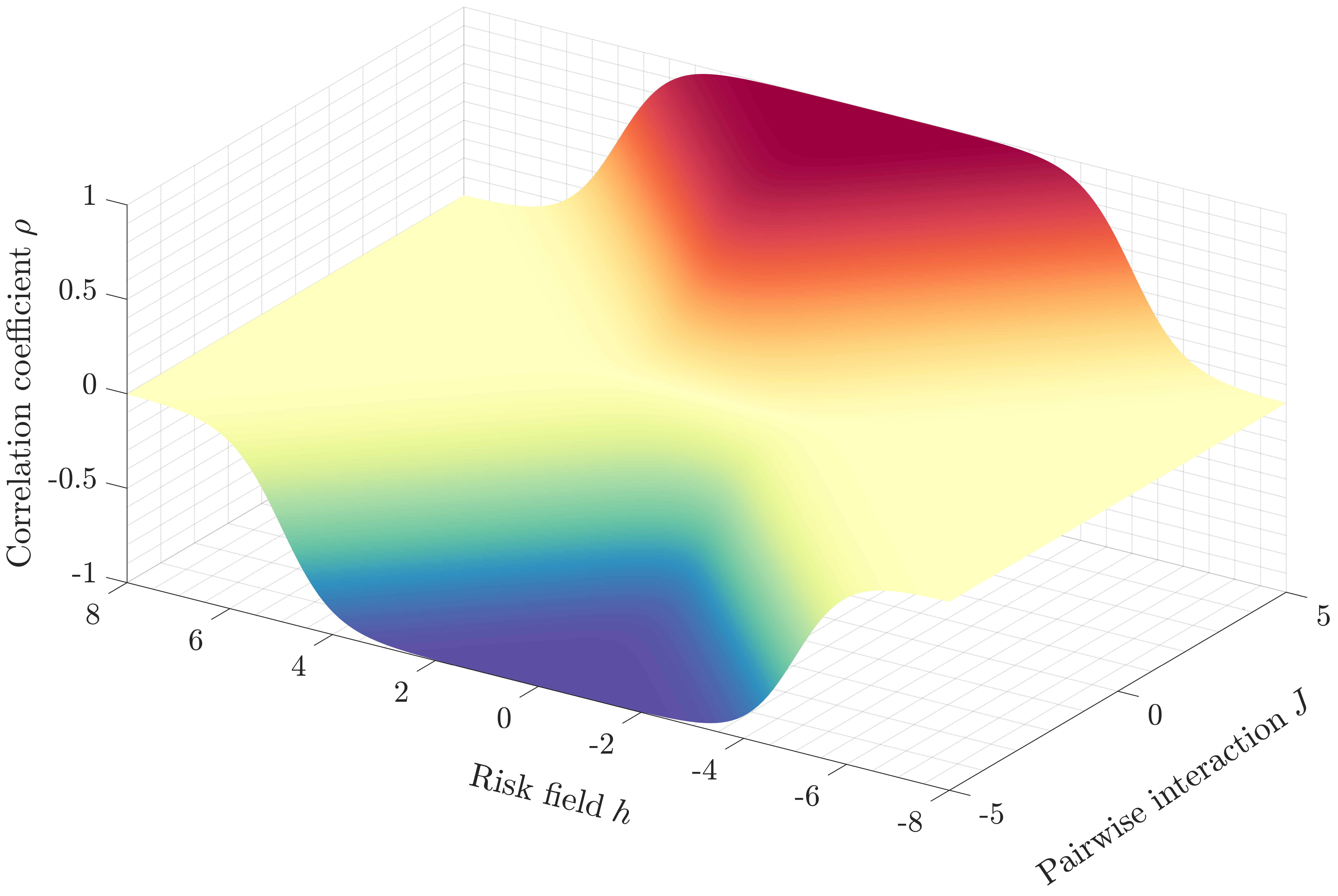
(a)

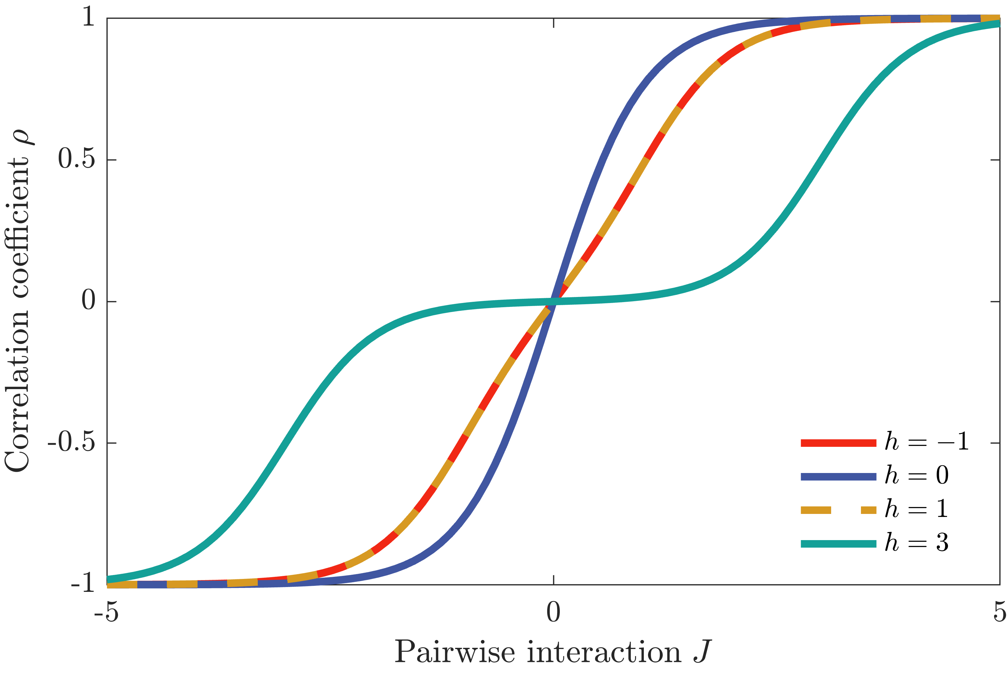
(b)

Figure 2: The relationship between the correlation coefficient $\rho$, risk field $h$, and pairwise interaction $J$ for two buildings: (a) three-dimensional representation, and (b) two-dimensional illustration of $\rho$ against $J$ for four $h$ values. For any $h$, the correlation coefficient $\rho$ is monotonically increasing with respect to $J$. A large $|h|$ flattens the increase, while a small $|h|$ steepens it.

To further investigate the relationship between the correlation coefficient and pairwise interaction, we consider a scenario involving three buildings without a risk field. Figure 3 shows the $J_{ij}$ values for each pair of buildings and the corresponding correlation coefficient values. Despite having no direct interaction, i.e., $J_{AB}=0$, buildings A and B exhibit a correlation coefficient of $0.58$. This is attributed to the significant pairwise interactions between buildings A and C and between buildings C and B. Additionally, Figures 4 demonstrates that buildings A and B have a zero correlation coefficient, despite a large positive $J$ value of $0.66$. This occurs because the indirect effects of the positive interaction between buildings A and C and the negative interaction between buildings B and C outweigh the direct interaction between buildings A and B.

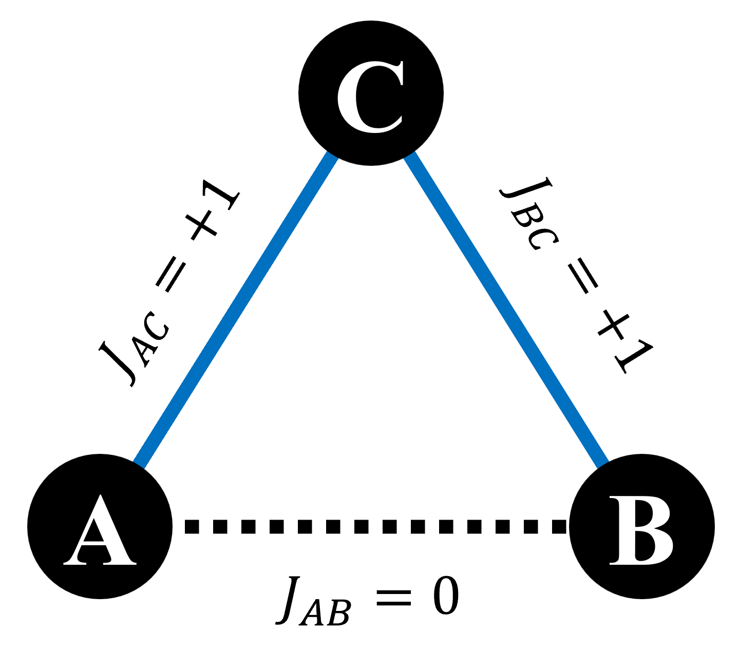
(a)

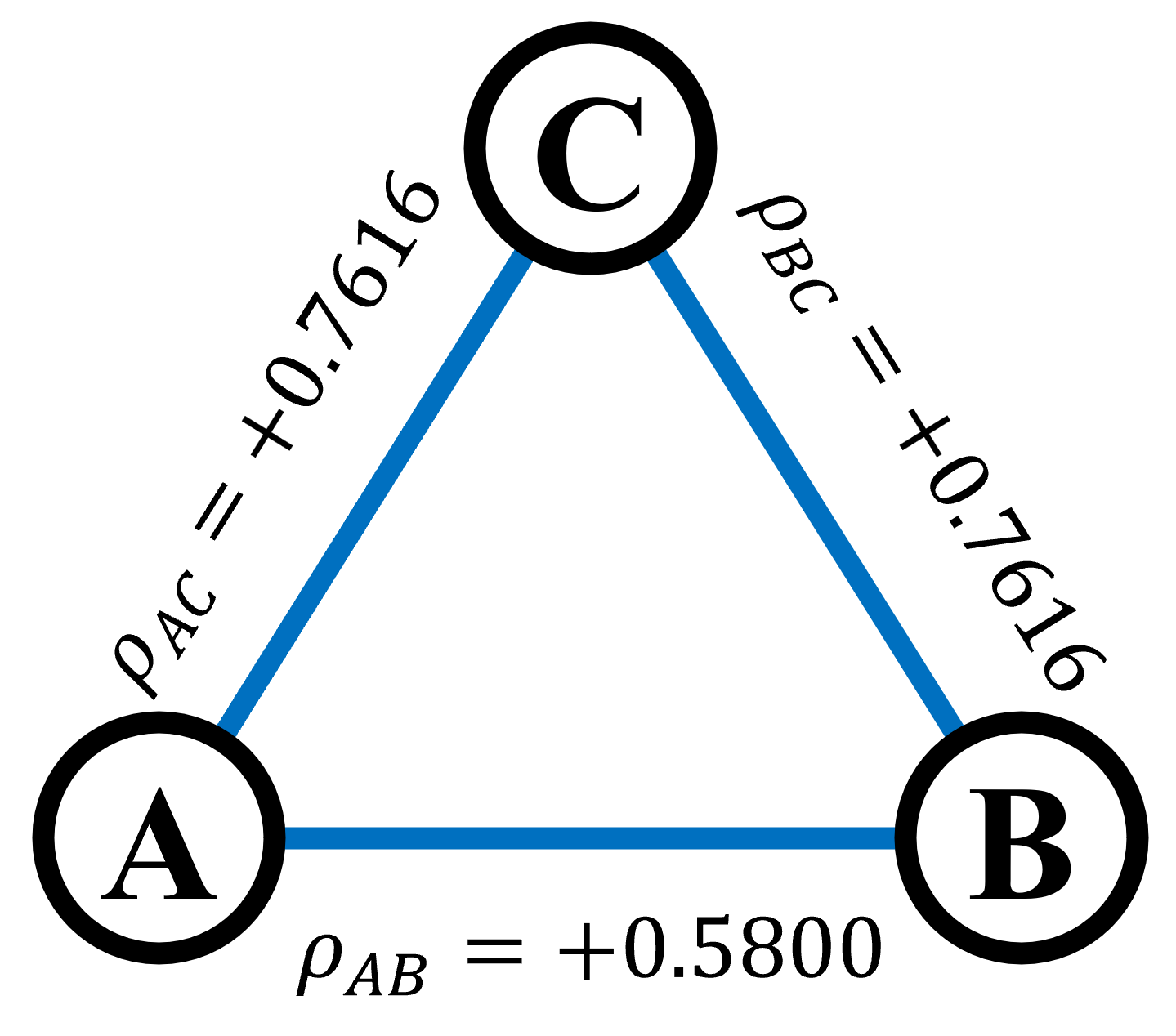
(b)

Figure 3: A 3-node system with zero pairwise interaction between nodes A and B: (a) the pairwise interaction values, and (b) the corresponding correlation coefficient values. A non-zero correlation coefficient does not necessarily imply a non-zero pairwise interaction.

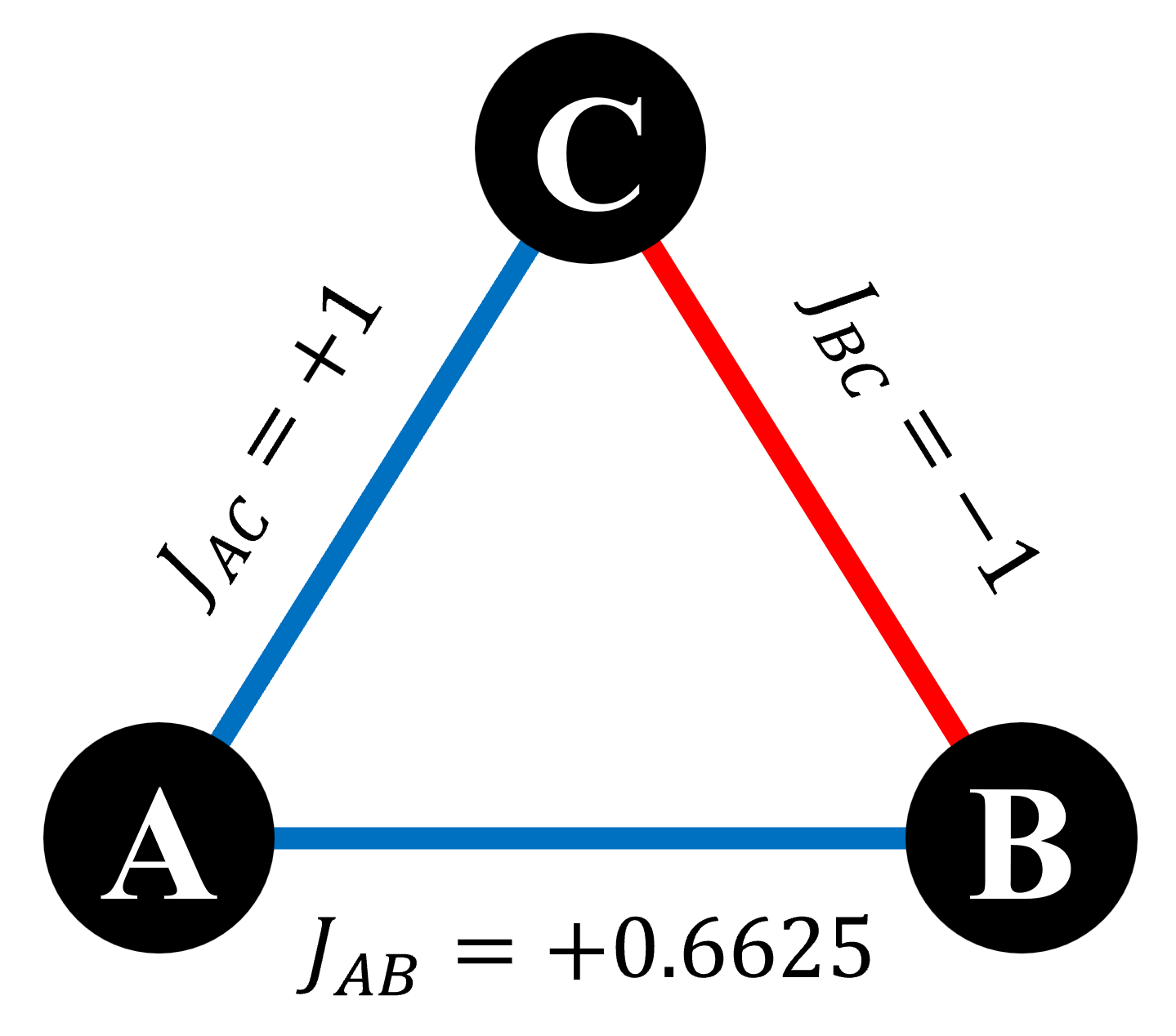
(a)

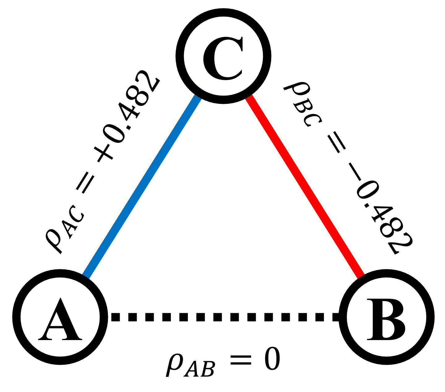
(b)

Figure 4: A 3-node system with zero correlation coefficient between nodes A and B: (a) the pairwise interaction values, and (b) the corresponding correlation coefficient values. A zero correlation coefficient does not necessarily suggest a zero pairwise interaction.

The illustrations above demonstrate the complex interplay between the Ising model parameters and both the mean and the correlation coefficient. The mean damage state of a structure is primarily influenced by the risk field acting on it, although the pairwise interactions also contribute to either sharpening or diminishing this effect. Similarly, the correlation coefficient for the damage states between a pair of structures is influenced by all pairwise interactions involving those structures, with the magnitude of the risk field either amplifying or mitigating this effect. These dynamics are approximately represented by the mean-field solutions in Eqs. (14) and (15). In essence, the Ising model, parameterized by $\boldsymbol{h}$ and $\boldsymbol{J}$, provides a fundamental mechanism for generating the mean damage states and correlation coefficients.

5 Numerical examples

This section investigates the engineering relevance of the Ising model in the context of regional seismic analysis. The data for constructing the Ising model, the first- and second-order cross-moments for damage states of structures, can be obtained from fragility curves and their correlation models [25]. This data can also be generated from regional seismic response simulators, such as the Regional Resilience Determination (R2D) tool of SimCenter [48] and the Interdependent Networked Community Resilience Modeling Environment (IN-CORE) platform of NCSA [49]. In this study, we first demonstrate how the Ising model can be built using post-earthquake damage evaluation data from a region in Antakya, Turkey, following the 2023 Turkey-Syria earthquake. Next, we construct the Ising model for a neighborhood in Pacific Heights, San Francisco, using samples generated by the R2D tool.

5.1 Example 1: Ising model from post-earthquake damage evaluation data

A neighborhood in Antakya, Turkey, is selected as the target region for constructing the Ising model. The data on building damages is obtained from the Humanitarian OpenStreetMap (HOTOSM) Team [50, 51]. Figure 5 illustrates the damage states for the target region following the 2023 Turkey-Syria earthquake. The region consists of 156 buildings, 40 of which failed during the earthquake.

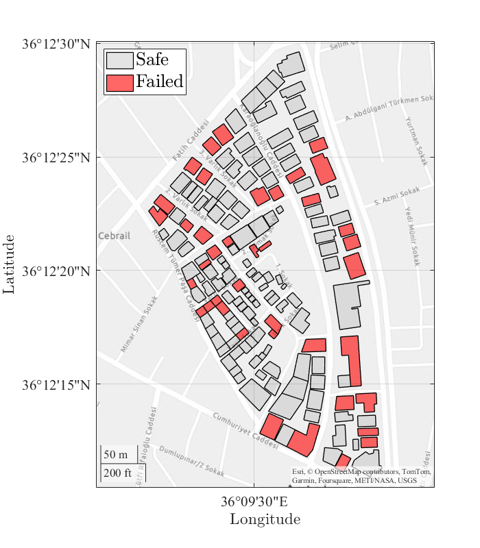
Figure 5: The building damages in a region of Antakya, Turkey, following the 2023 Turkey-Syria earthquake.

To construct the Ising model, we use the following information: the total number of failed buildings, which is 40 out of 156, and the correlation coefficients between each building pair. Given that we have only a single observation under the earthquake event, we assume spatial ergodicity to obtain the correlation coefficients. Specifically, a correlation coefficient function $\rho(d)$, where $d$ is the distance between two buildings, is fitted to the correlation coefficient values derived by spatially averaging the data. The regression law is found to be $\rho(d)={1}/{\left(1+94.9073d\right)}$, which closely matches the data, as illustrated in Figure 6.

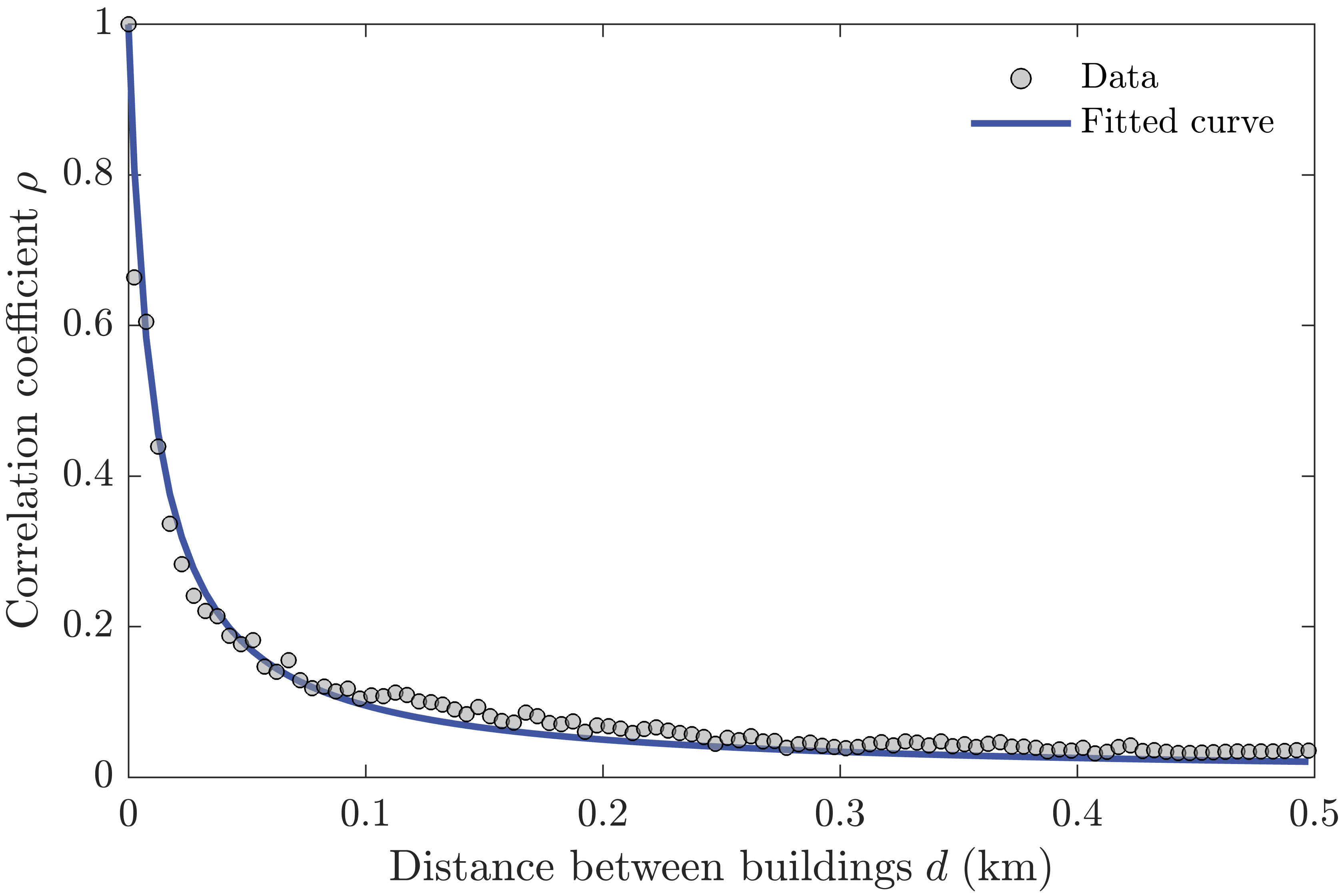
Figure 6: The correlation coefficient function $\rho(d)$ fitted to the spatially averaged correlation coefficient values calculated at each distance bin.

The Ising model is then constructed by Boltzmann machine learning. Figure 7 illustrates the estimated Ising model parameters. Note that we have only one $h$ representing the risk field averaged over the region, rather than a fine-grained $h_{i}$ for each building. This is consistent with the limited prior information—the total number of failed buildings.

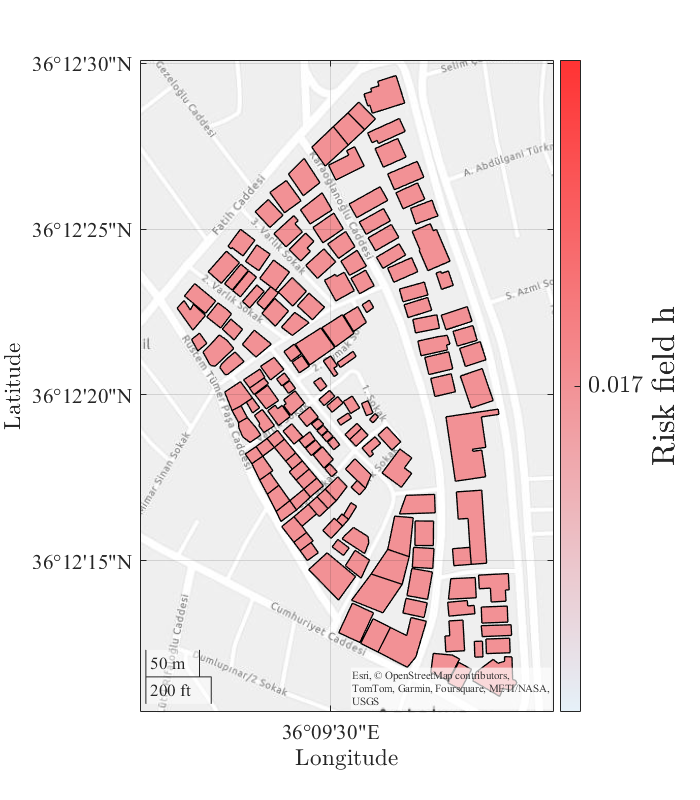
(a)

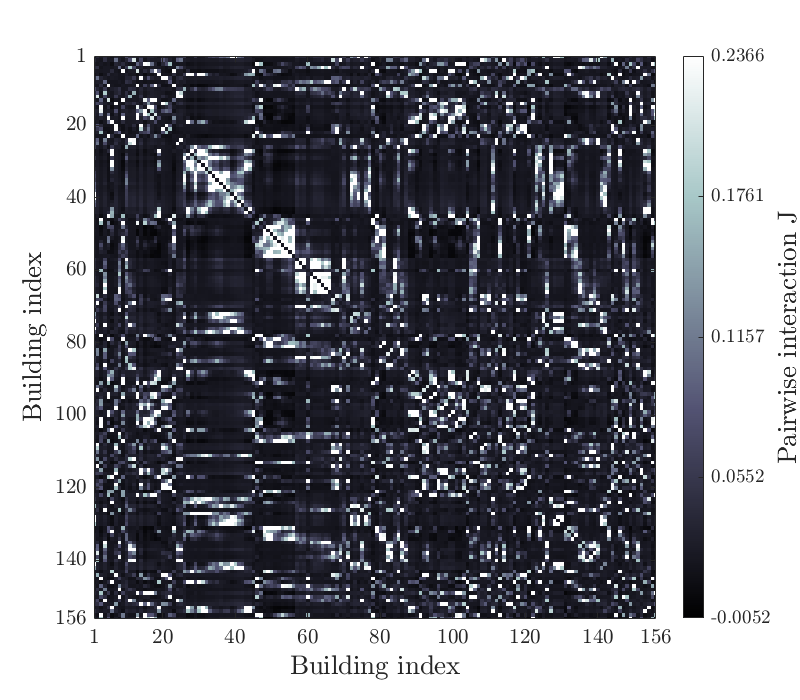
(b)

Figure 7: The estimated Ising model parameters for Antakya, Turkey, following the 2023 Turkey-Syria earthquake: (a) averaged risk field $h$ and (b) pairwise interaction $\boldsymbol{J}$. Due to the limited prior information, only a single $h$ representing the average risk field is obtained. However, $\boldsymbol{J}$ includes interactions for all pairs of buildings, facilitated by the correlation function $\rho(d)$.

The constructed Ising model reproduces the expected number of failed buildings as 39 (technically, 38.9781), which is close to the observed 40. The validity of the constructed Ising model in terms of reproducing the input information can also be seen in Figure 8. The correlation coefficients reproduced using the Ising model, shown as Figure 8(b), are close to the given values presented in Figure 8(a). It is also noteworthy that the pattern of pairwise interactions closely resembles that of the given correlation coefficients. This suggests that, based on the limited observational data, the correlation coefficients between damages of buildings primarily arise from pairwise interactions between buildings rather than from the risk field.

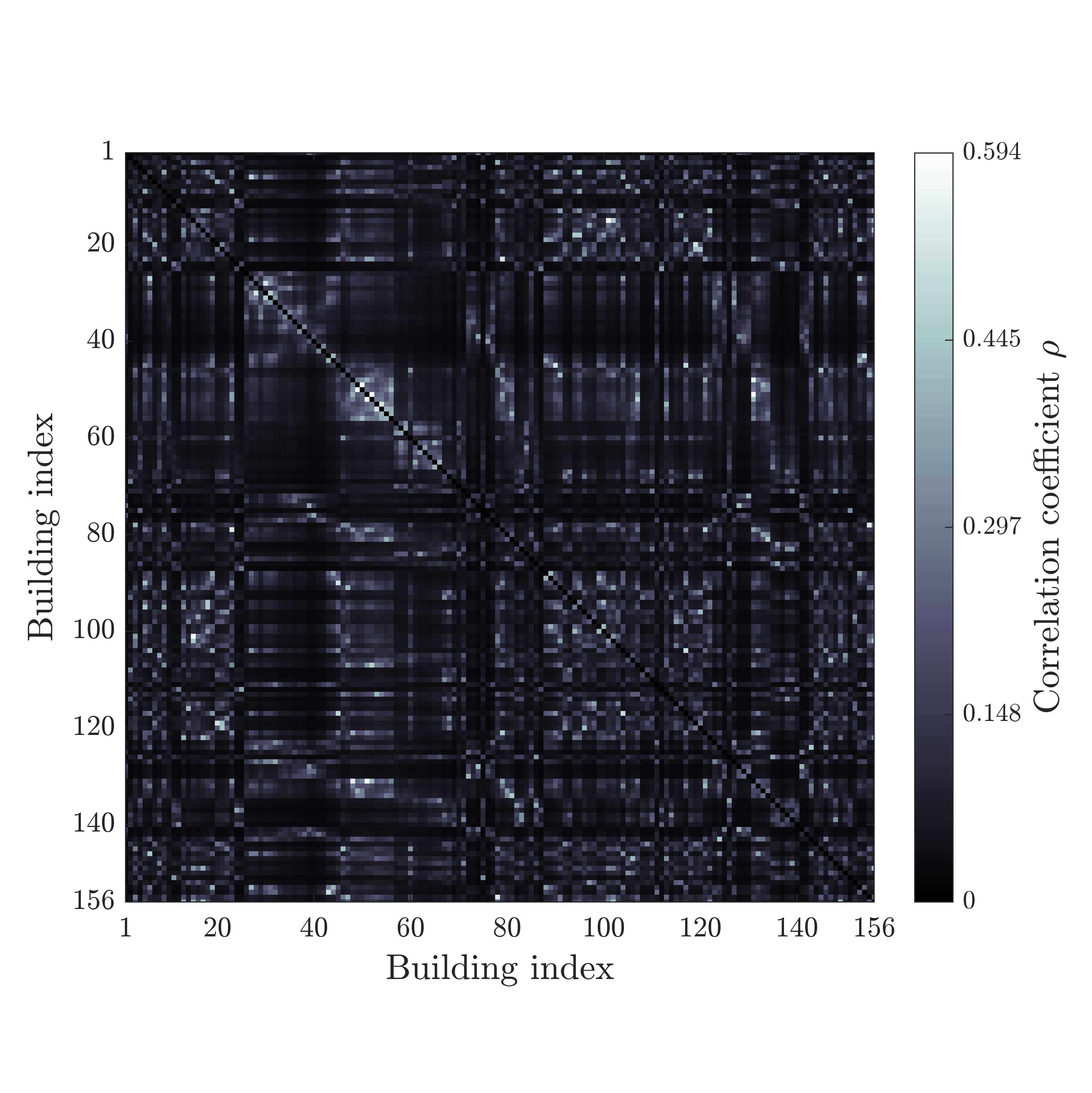
(a)

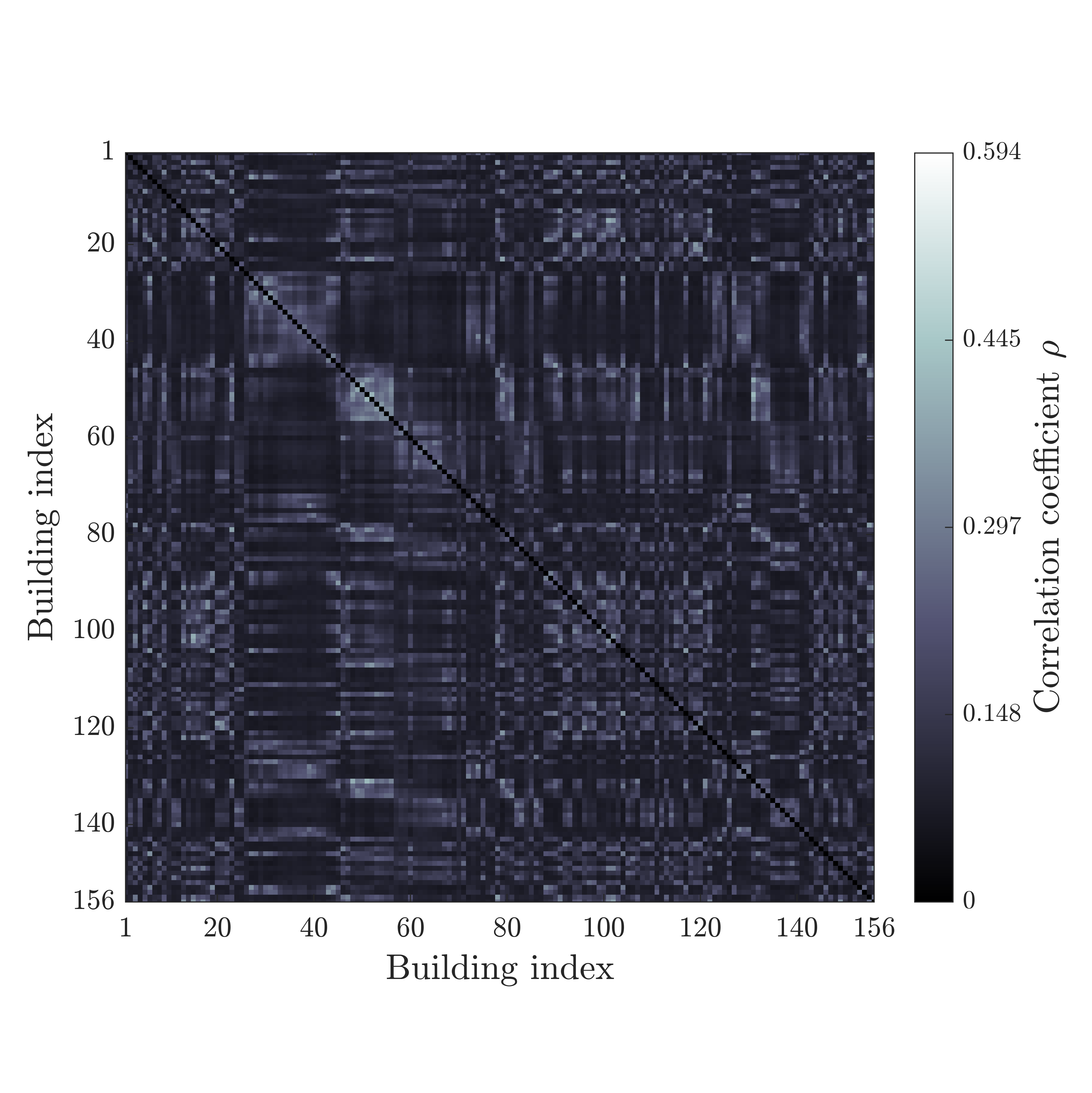
(b)

Figure 8: Correlation coefficients between each building pair in the target region: (a) calculated from the observation, and (b) reproduced using the Ising model. The two panels exhibit similar patterns. To enhance the visualization of pairwise correlations, the diagonal terms are excluded.

The Ising model represents a joint probability distribution for all modeled structures over a region, providing a complete statistical description. Using the model, a total of $10^{7}$ samples is generated. The failure probability for each building is then obtained, as illustrated in Figure 9. Figure 9 shows that closely spaced buildings exhibit an overall higher failure probability. This is because the risk field is identical for all buildings, whereas the pairwise interactions are stronger in denser regions. It is important to note that the failure probabilities presented in Figure 9 are predictions of the Ising model based on the current state of knowledge.

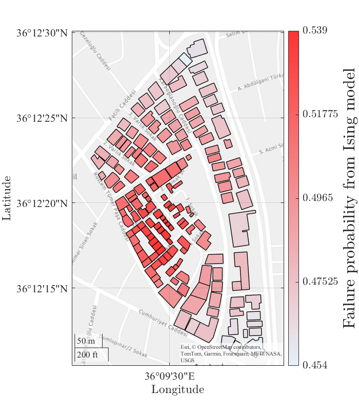
Figure 9: Failure probability of each building predicted by the Ising model. This prediction is based on the current state of knowledge.

Figure 10 illustrates a histogram of the number of failed buildings from the $10^{7}$ samples. It is observed that the mode (most probable number of failed buildings) is around 25, although the expected number is 39. Moreover, the probability of more than 100 buildings will fail is 3.85%, which is not negligible. This is because the distribution of the number of failed buildings has a long right tail. Indeed, it is well known that the Ising model exhibits bimodal for the global mean-field (number of failed buildings in this example) when pairwise interactions are large [28]. Although bimodality is only noticeable in Figure 10, in regions with higher correlation coefficients, such as residential zones with similar houses, the bimodality would be more pronounced and a collective failure would be non-negligible.

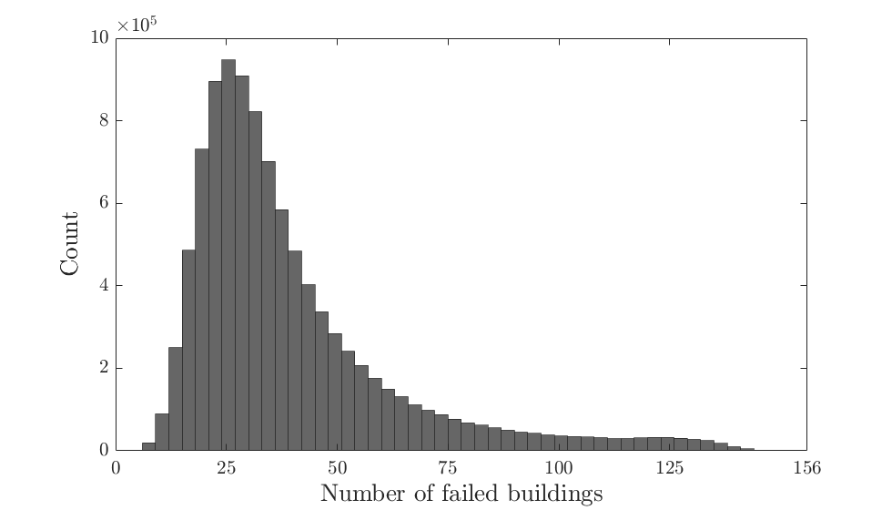
Figure 10: Histogram of the number of failed buildings predicted by the Ising model. The distribution features a long right tail with a small, yet noticeable, second mode.

5.2 Example 2: Ising model based on fragility functions

In this example, the Ising model is constructed from samples generated by the R2D tool provided by the NHERI SimCenter. A neighborhood in Pacific Heights, San Francisco, is chosen as the modeled region, containing 182 buildings. A earthquake scenario of magnitude 7.0 is assumed. The epicenter is on the San Andreas Fault, at latitude 37.9, longitude -122.432, with a depth of 80 kilometers. Given the earthquake scenario, the R2D computes peak ground accelerations (PGA) at each building site using the ground motion prediction equation (GMPE) developed in Boore et al. [12]. The models from Baker and Jayaram [52] and Markhvida et al. [53] are used to account for the inter- and intra-event spatial correlations in PGAs, respectively. Given the PGA values at each building site, the damage state for each building is evaluated using fragility curves provided by Hazus [54], leveraging structural information integrated into the R2D tool. This includes geographical location, plan area, year built, number of stories, and structural type of the buildings. Due to limitations in the current R2D tool, correlations between the capacities of buildings are not considered. Subsequently, 10,000 samples are generated, each sample being a vector representing the damage states for the 182 buildings.

Using the samples, we obtain the failure probability for each building and the correlation coefficient matrix of the damage states. The Ising model parameters are then estimated. Figure 11 shows a comparison between the given statistics and those reproduced by the Ising model. It is observed that the Ising model accurately reproduces the given statistics.

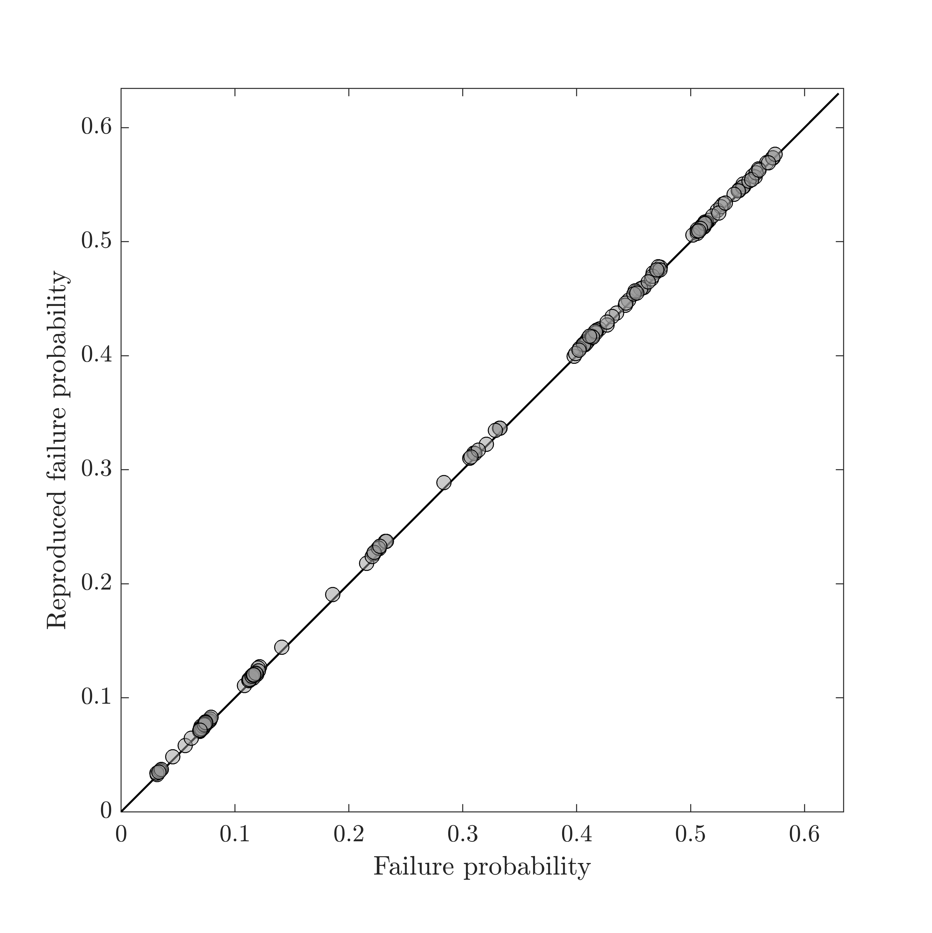
(a)

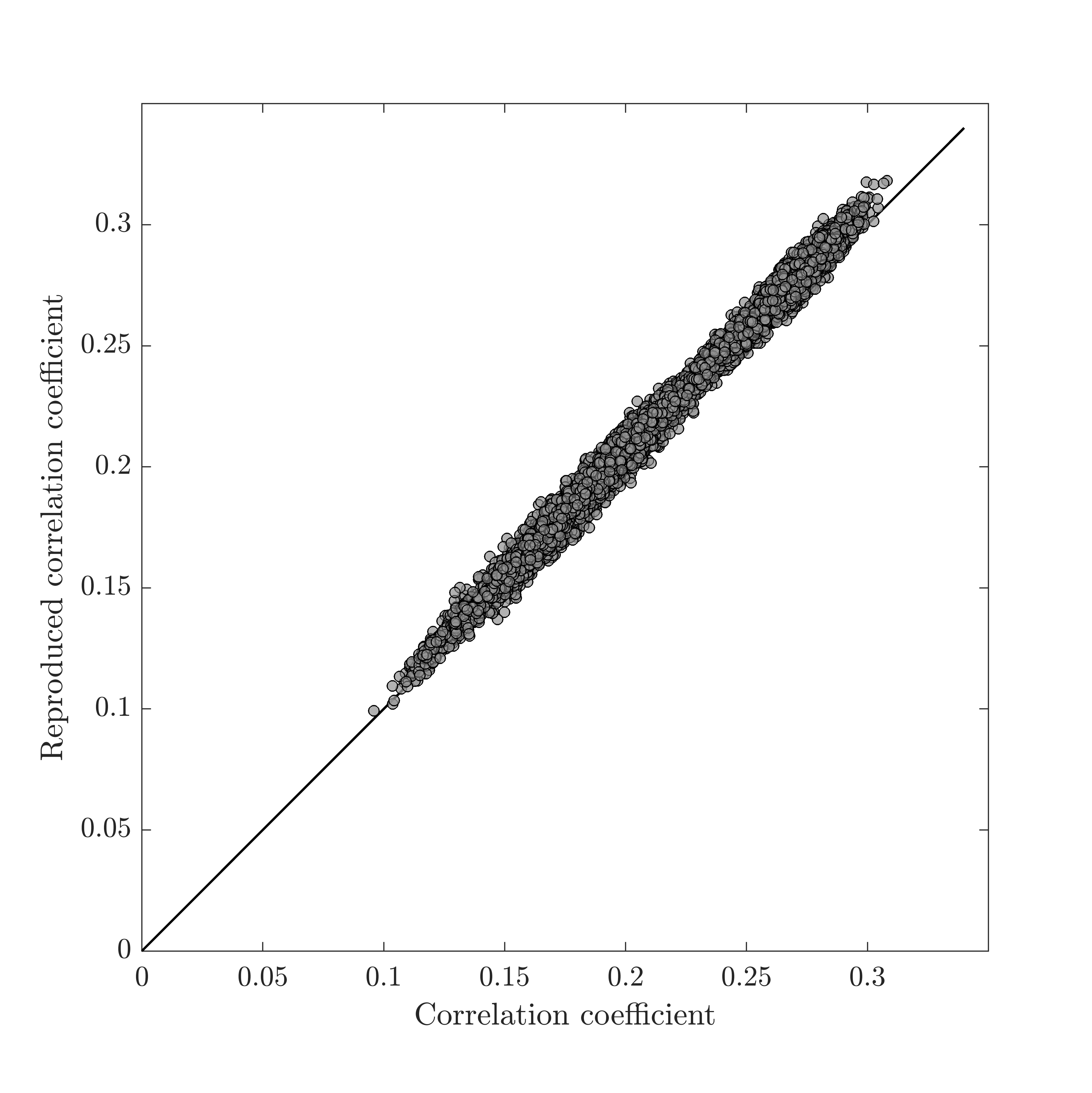
(b)

Figure 11: Comparison between the given statistics and those reproduced by the Ising model: (a) failure probability, and (b) correlation coefficient. The solid diagonal line signifies perfect reconstruction.

Figure 12 compares the failure probabilities provided by the R2D tool with the risk field values derived from the Ising model, with the color bars min-max normalized. Notably, if we rank the risks of the buildings according to their failure probabilities and compare these rankings to those based on risk field values, the rankings would differ, as illustrated in Figure 13. Specifically, some buildings are considered more risky based on their failure probabilities than their risk field values, while others are viewed as riskier based on the risk field values. This discrepancy can be revealed by their differences in pairwise interactions $\boldsymbol{J}$, as depicted in Figure 14. For instance, building indexed as 108 stands out in Figure 13 for being below and far from the reference line of equal ranking. From Figure 14, it is noted that building #108 also deviates from the rest by having the lowest average interaction with other buildings. This indicates that, in contrast to other buildings which are more likely to fail alongside their close neighborhoods, building #108 exhibits relatively weaker interaction with others. Therefore, contrasting the risk field $\boldsymbol{h}$ with individual failure probabilities reveals the impact of “collective behavior” among structures. This observation is supported by the mean-field approximation in Eq. (16), where the discrepancy between $h_{i}$ and $m_{i}$ reflects the effect of interactions.

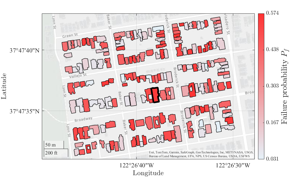
(a)

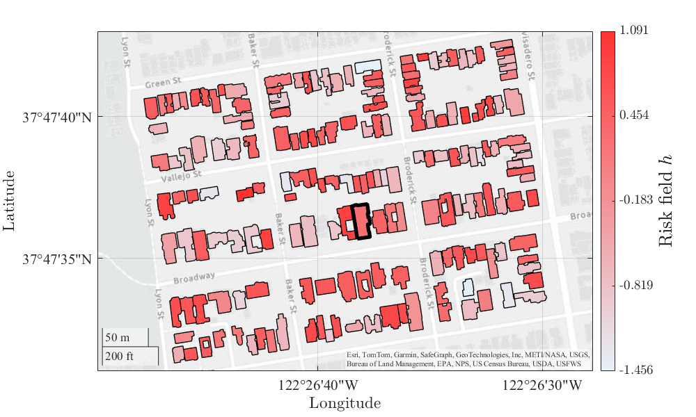
(b)

Figure 12: Illustrations of (a) the failure probabilities and (b) the risk field $\boldsymbol{h}$ values for each building in Pacific Heights, San Francisco. Building #108, which is of particular importance, is highlighted by a bold black solid line.

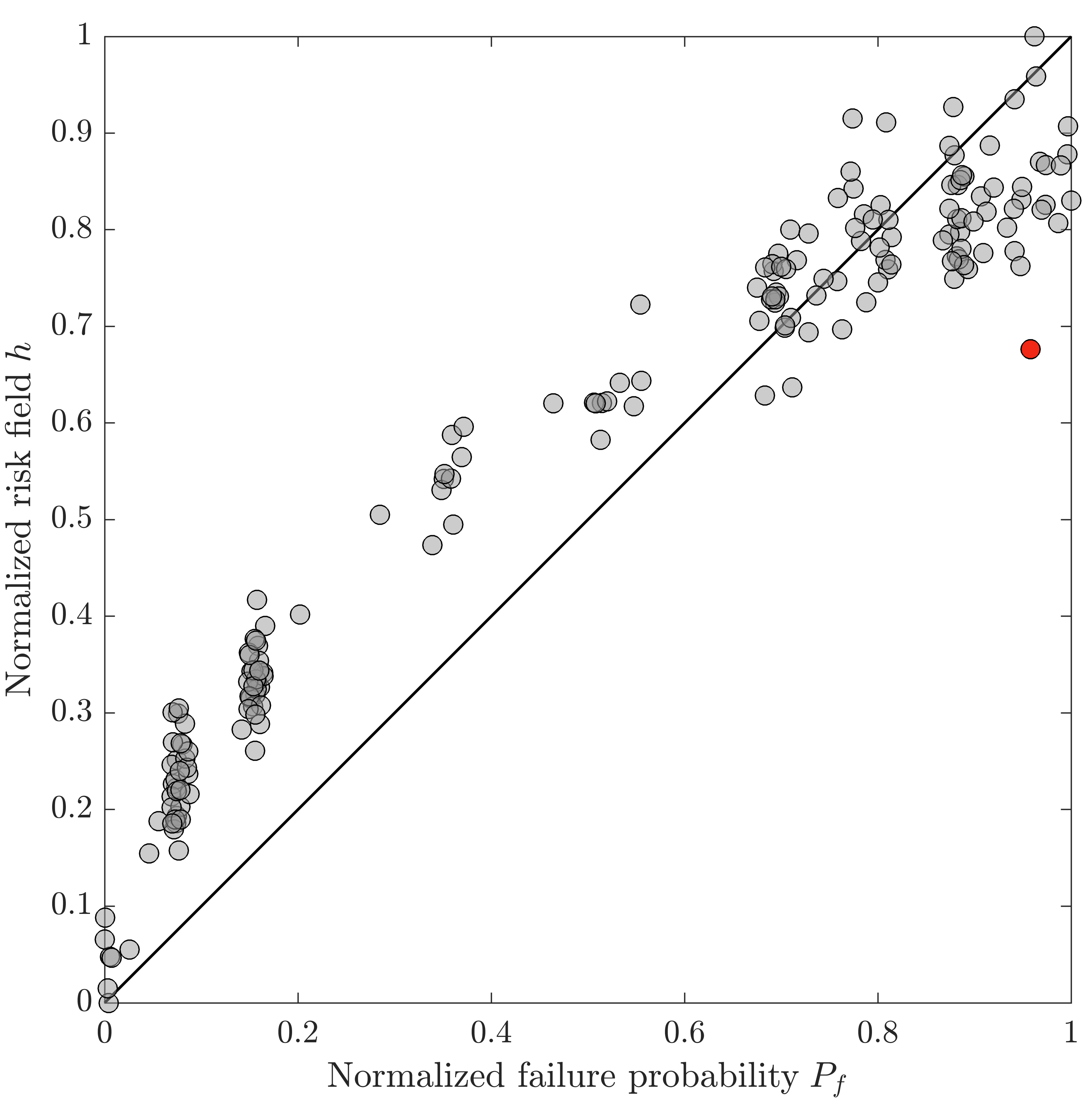
Figure 13: Comparison of the normalized risk field and the normalized failure probabilities. The values are min-max normalized. The black solid line represents the reference for equal ranking by risk field and failure probability. Building #108, marked by red, is identified as an “outlier” because it deviates significantly from the reference line of equal ranking.

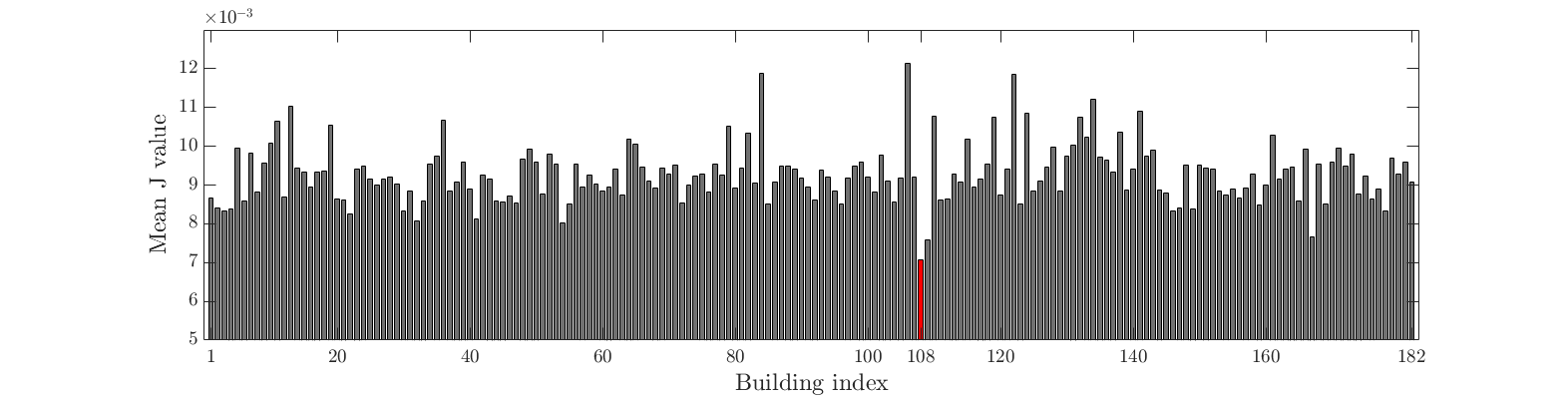
Figure 14: The average pairwise interaction value for each building. For the $i$-th building, we average its interaction with other buildings to obtain $\sum_{j}J_{ij}/n$. The average interaction for building # 108 is highlighted in red.

Lastly, we examine the relationship between the risk field and earthquake magnitudes. Beyond the existing scenario of magnitude $7.0$, we construct Ising models for earthquake magnitudes of $6.0$, $8.0$, and $9.0$. The results, presented in Figure 15, show that the right/positive mode of $h_{i}$ becomes more dominant as the magnitude increases. The left/negative mode of $h_{i}$ persists across all magnitudes. This is because the mean failure probability is around $0.5$ even at a magnitude of $9.0$, suggesting a significant inertia towards remaining safe, i.e., negative $h_{i}$, among many structures. The relationship between the pairwise interaction and earthquake magnitudes is illustrated by Figure 16. The results suggest that the dispersion of $J_{ij}$ decreases as the magnitude increases, but the spatial mean of $J_{ij}$ across all pairs is not sensitive to the magnitude. This weak dependency between $\boldsymbol{J}$ and magnitude may be attributed to the fact that $\boldsymbol{J}$ primarily reflects the inherent interdependencies among structures.

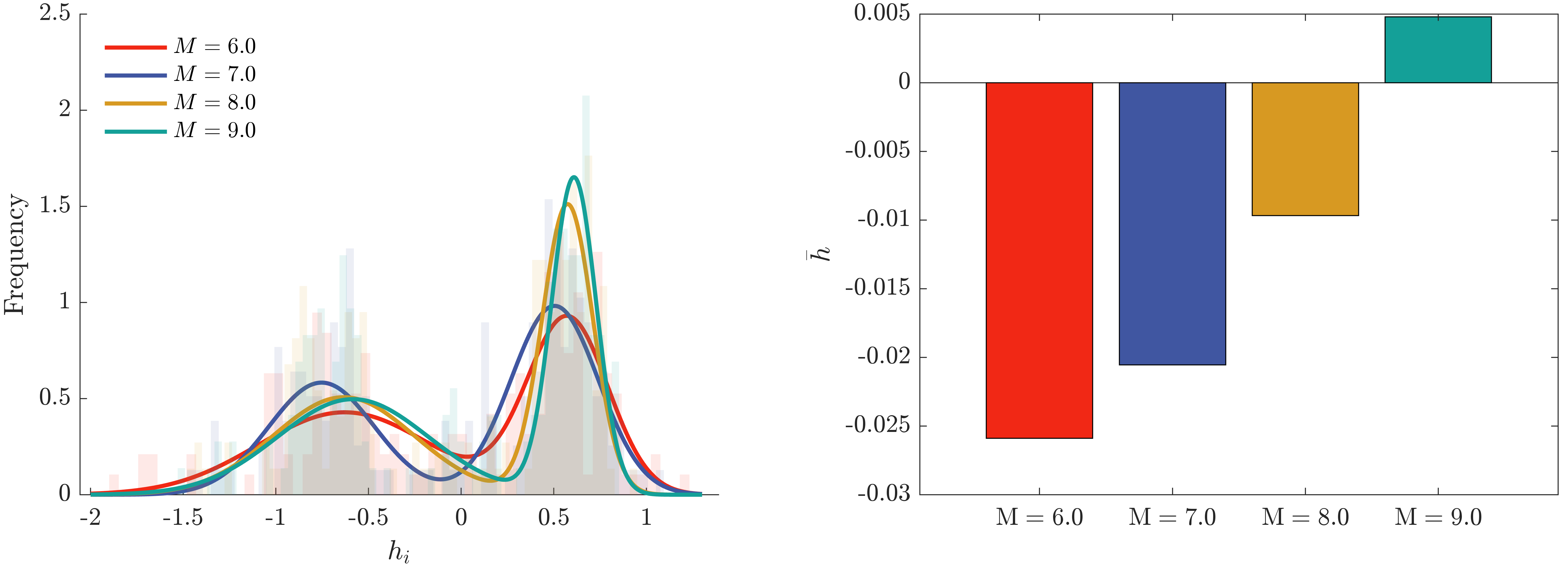
Figure 15: The relationship between the risk field $\boldsymbol{h}$ and earthquake magnitude. The left panel shows the histogram of $h_{i}$ for four earthquake magnitudes, while the right panel illustrates the spatial mean of $h_{i}$, $\bar{h}=\sum_{i}h_{i}/n$. It is observed that the positive mode of $h_{i}$ becomes more pronounced with increasing earthquake magnitude. Additionally, the spatial mean $\bar{h}$, which is proportional to the probability of all structures collectively failing, monotonically increases with magnitude.

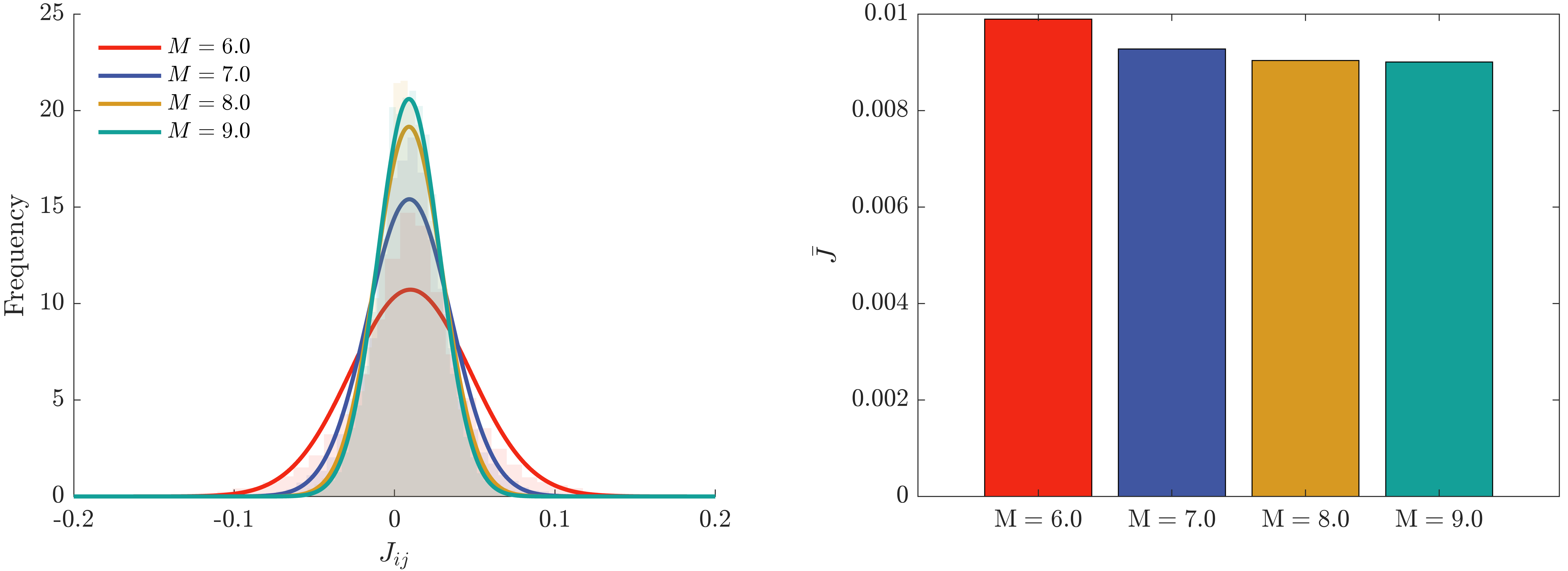
Figure 16: The relationship between the pairwise interaction $\boldsymbol{J}$ and earthquake magnitude. The left panel shows the histogram of $J_{ij}$ for four earthquake magnitudes, while the right panel illustrates the spatial mean of $J_{ij}$, $\bar{J}=\sum_{ij}J_{ij}/n^{2}$. It is observed that $J_{ij}$ becomes more concentrated with increasing earthquake magnitude, while $\bar{J}$ decreases slowly with magnitude.

6 Conclusions

This study introduces the long-range Ising model as a joint probability distribution of damage states of structures for regional seismic simulations. Using the principle of maximum entropy, the long-range Ising model is derived under the constraints of the first- and second-order cross-moments of the damage states. The Ising model parameters, $\boldsymbol{h}$ and $\boldsymbol{J}$, are interpreted as a risk field acting at each structure and the pairwise interaction between structures, respectively. Through simple demonstrative examples, the complex interplay between the Ising model parameters and the mean and correlation coefficient of damage states is illustrated. It is found that the mean damage state of a structure is primarily influenced by the risk field acting on it, although the pairwise interactions also play a role in either sharpening or diminishing this effect. Similarly, the correlation coefficient for the damage states between a pair of structures is influenced by all pairwise interactions involving those structures, with the magnitude of the risk field either amplifying or mitigating this effect. The engineering relevance of the Ising model is further illustrated by two simulation test cases. The first example considers the damage states of buildings in Antakya, Turkey, following the 2023 Turkey-Syria earthquake, the second example studies neighborhood in Pacific Heights, San Francisco, under sythetic earthquake scenarios generated by the Regional Resilience Determination (R2D) tool of the NHERI SimCenter. It is found that for both examples the Ising model can reproduce the given information. More importantly, the Ising model offers insights on the collective behavior of structural failures. Specifically, it is found that the discrepancy between the rankings provided by the individual failure probabilities and the risk field values signifies the impact of collective behavior of failing/not-failing together.

The Ising model serves as a fundamental component for more advanced statistical mechanics methods to analyze the multi-scale behaviors, phase transitions, and scaling laws in complex multi-body systems. This work establishes a basis for further extensions, suggesting several promising research directions:

• Development of Renormalization Group [28] method for modeling and understanding the multi-scale behavior of regional seismic responses.

• Early-warning systems for system-level phase transitions and criticality.

• Ising models for functionalities of civil infrastructures.

• Regression models linking ground motion intensity measures to Ising model parameters.

• Development of efficient computational methods for estimating Ising model parameters.

Appendix A Derivation of the Ising model using the principle of maximum entropy

The goal is to find the joint probability $P_{I}$ that meets the given constraints and also maximizes the entropy. Applying Lagrange multipliers for the constraints described in Eqs. (5) and (6), maximizing the entropy $S$ is equivalent to maximizing:

$$L= -\sum_{I=1}^{N}P_{I}\log{P_{I}}-\alpha\left(1-\sum_{I=1}^{N}P_{I}\right)$$ (17)

$$-\sum_{i=1}^{n}h_{i}\left(\mathcal{M}_{1,i}-\sum_{I=1}^{N}x_{iI}P_{I}\right)-\sum_{i>j}J_{ij}\left(\mathcal{M}_{2,ij}-\sum_{I=1}^{N}x_{iI}x_{jI}P_{I}\right)\,,$$

where $\alpha$, $h_{i}$, and $J_{ij}$ are Lagrange multipliers. Taking the partial derivative of Eq. (17) with respect to $P_{I}$, we obtain:

$$\frac{\partial L}{\partial P_{I}}=-\log{P_{I}}-1+\alpha+\sum_{i=1}^{n}h_{i}x_{iI}+\sum_{i>j}J_{ij}x_{iI}x_{jI}\,.$$ (18)

Finally, we obtain $P_{I}$ that meets $\frac{\partial S}{\partial P_{I}}=0$ as follows:

$$P_{I} =\exp{\left(-1+\alpha+\sum_{i=1}^{n}h_{i}x_{iI}+\sum_{i>j}J_{ij}x_{iI}x_{jI}\right)}$$

$$=\frac{1}{Z}\exp{\left(\sum_{i=1}^{n}h_{i}x_{iI}+\sum_{i>j}J_{ij}x_{iI}x_{jI}\right)}\,,$$

where $Z=\exp{\left(1-\alpha\right)}$.

Appendix B Derivation of the mean-field approximation

The mean-field approximation assumes that the fluctuation in each component is relatively small compared with its mean-field [55]. Then, $x_{i}x_{j}$ can be approximated by:

$$x_{i}x_{j} =\left(m_{i}+\left(x_{i}-m_{i}\right)\right)\left(m_{j}+\left(x_{i}-m_{i}\right)\right)$$ (19)

$$\approx m_{i}m_{j}+m_{i}\left(x_{j}-m_{j}\right)+m_{j}\left(x_{i}-m_{i}\right)$$

$$=m_{i}x_{j}+m_{j}x_{i}-m_{i}m_{j}\,.$$

Subsequently, the normalizing constant $Z$ can be expressed by:

$$Z =\sum_{I}\exp{\left(\sum_{i=1}^{n}h_{i}x_{i}+\sum_{i>j}J_{ij}x_{i}x_{j}\right)}$$ (20)

$$\approx\sum_{I}\exp{\left(\sum_{i=1}^{n}h_{i}x_{i}+\sum_{i>j}J_{ij}m_{i}x_{j}+\sum_{i>j}J_{ij}m_{j}x_{i}-\sum_{i>j}J_{ij}m_{i}m_{j}\right)}$$

$$=\sum_{I}\exp{\left(\sum_{i=1}^{n}h_{i}x_{i}+\sum_{i\neq j}J_{ij}m_{j}x_{i}-\frac{1}{2}\sum_{i\neq j}J_{ij}m_{i}m_{j}\right)}$$

$$=\sum_{I}\exp{\left(\sum_{i=1}^{n}\tilde{h}_{i}x_{i}-\frac{1}{2}\sum_{i\neq j}J_{ij}m_{i}m_{j}\right)}.$$

$$=c\sum_{I}\exp{\left(\sum_{i=1}^{n}\tilde{h}_{i}x_{i}\right)}\,,$$

where $\tilde{h}_{i}=h_{i}+\sum_{j\neq i}J_{ij}m_{j}$ is the effective external field that incorporates the effect of pairwise interactions, and $c\equiv\exp\left(-\frac{1}{2}\sum_{i\neq j}J_{ij}m_{i}m_{j}\right)$ is introduced for brevity. The symmetry of $\boldsymbol{J}$, $J_{ij}=J_{ji}$, was used for the third line of the equation. We further simplify $Z$ into:

$$Z =c\sum_{I}\prod_{i=1}^{n}\exp{\tilde{h}_{i}x_{i}}$$ (21)

$$=c\prod_{i=1}^{n}\left(\exp(\tilde{h}_{i})+\exp(-\tilde{h}_{i})\right)$$

$$=c\prod_{i=1}^{n}2\cosh{\tilde{h}_{i}}\,,$$

which is followed by

$$\ln{Z}=\ln c+n\ln{2}+\sum_{i=1}^{n}\ln{\cosh{\tilde{h}_{i}}}\,.$$ (22)

Finally, using the properties of $m_{i}=\frac{\partial\ln{Z}}{\partial h_{i}}$ and $c_{ij}=\frac{\partial\ln{Z}}{\partial J_{ij}}=\frac{\partial m_{i}}{\partial h_{j}}$, the self-consistent equations for $m_{i}$ and $c_{ij}$ are derived as

$$m_{i} =\frac{\partial\ln{Z}}{\partial h_{i}}$$ (23)

$$=\tanh\left(\tilde{h}_{i}\right)$$

$$=\tanh\left({h_{i}+\sum_{j\neq i}J_{ij}m_{j}}\right)$$

$$c_{ij} =\frac{\partial m_{i}}{\partial h_{j}}$$

$$=\left(1-m_{i}^{2}\right)\left(\delta_{ij}+\sum_{k\neq i}J_{ik}c_{kj}\right)\,.$$

References

- Moehle and Deierlein [2004] Jack Moehle and Gregory G Deierlein. A framework methodology for performance-based earthquake engineering. In 13th World Conference on Earthquake Engineering, Vancouver, 2004. URL https://www.researchgate.net/publication/228706335.
- Porter [2003] Keith A Porter. An Overview of PEER’s Performance-Based Earthquake Engineering Methodology. In The 9th International Conference on Applications of Statistics and Probability in Civil Engineering (ICASP 9), San Francisco, 7 2003.
- Qiu and Zhu [2017] Can Xing Qiu and Songye Zhu. Performance-based seismic design of self-centering steel frames with SMA-based braces. Engineering Structures, 130:67–82, 1 2017. ISSN 18737323. doi: 10.1016/j.engstruct.2016.09.051.
- Zhang et al. [2018] Yu Zhang, Henry V. Burton, Han Sun, and Mehrdad Shokrabadi. A machine learning framework for assessing post-earthquake structural safety. Structural Safety, 72:1–16, 5 2018. ISSN 01674730. doi: 10.1016/j.strusafe.2017.12.001.
- Haselton and Deierlein [2007] Curt B Haselton and Gregory G Deierlein. Assessing Seismic Collapse Safety of Modern Reinforced Concrete Moment-Frame Buildings. Technical report, Pacific Earthquake Engineering Research Center, 8 2007.
- Li et al. [2020] Yaohan Li, You Dong, Dan M. Frangopol, and Dipendra Gautam. Long-term resilience and loss assessment of highway bridges under multiple natural hazards. Structure and Infrastructure Engineering, 16(4):626–641, 4 2020. ISSN 17448980. doi: 10.1080/15732479.2019.1699936.
- Heresi and Miranda [2023] Pablo Heresi and Eduardo Miranda. RPBEE: Performance-based earthquake engineering on a regional scale. Earthquake Spectra, 2023. ISSN 19448201. doi: 10.1177/87552930231179491.
- De Risi et al. [2018] Raffaele De Risi, Flavia De Luca, Oh-Sung Kwon, and Anastasios Sextos. Scenario-Based Seismic Risk Assessment for Buried Transmission Gas Pipelines at Regional Scale. Journal of Pipeline Systems Engineering and Practice, 9(4), 11 2018. ISSN 1949-1190. doi: 10.1061/(asce)ps.1949-1204.0000330.
- Hulsey et al. [2022] Anne M. Hulsey, Jack W. Baker, and Gregory G. Deierlein. High-resolution post-earthquake recovery simulation: Impact of safety cordons. Earthquake Spectra, 38(3):2061–2087, 8 2022. ISSN 19448201. doi: 10.1177/87552930221075364.
- Zhang et al. [2023] Wenyang Zhang, Peng Yu Chen, Jorge G.F. Crempien, Asli Kurtulus, Pedro Arduino, and Ertugrul Taciroglu. Regional-scale seismic fragility, loss, and resilience assessment using physics-based simulated ground motions: An application to Istanbul. Earthquake Engineering and Structural Dynamics, 52(6):1785–1804, 5 2023. ISSN 10969845. doi: 10.1002/eqe.3843.
- Rodgers et al. [2019] Arthur J. Rodgers, Arben Pitarka, N. Anders Petersson, Bjorn Sjogreen, David B. McCallen, and Norman Abrahamson. Broadband (0-5 Hz) fully deterministic 3D ground-motion simulations of a magnitude 7.0 Hayward fault earthquake: Comparison with empirical ground-motion models and 3D path and site effects from source normalized intensities. Seismological Research Letters, 90(3):1268–1284, 2019. ISSN 19382057. doi: 10.1785/0220180261.
- Boore et al. [2014] David M. Boore, Jonathan P. Stewart, Emel Seyhan, and Gail M. Atkinson. NGA-West2 equations for predicting PGA, PGV, and 5% damped PSA for shallow crustal earthquakes. Earthquake Spectra, 30(3):1057–1085, 8 2014. ISSN 19448201. doi: 10.1193/070113EQS184M.
- Cornell et al. [2002] Allin Cornell, M Asce, Fatemeh Jalayer, Ronald O Hamburger, and Douglas A Foutch. Probabilistic Basis for 2000 SAC Federal Emergency Management Agency Steel Moment Frame Guidelines. Journal of structural engineering, 128(4):526–533, 2002. doi: 10.1061/ASCE0733-94452002128:4526.
- Heresi and Miranda [2021] Pablo Heresi and Eduardo Miranda. Fragility Curves and Methodology for Estimating Postearthquake Occupancy of Wood-Frame Single-Family Houses on a Regional Scale. Journal of Structural Engineering, 147(5), 5 2021. ISSN 0733-9445. doi: 10.1061/(asce)st.1943-541x.0002989.
- Esmaili et al. [2018] Omid Esmaili, Lisa Grant Ludwig, and Farzin Zareian. An Applied Method for General Regional Seismic Loss Assessment—With A Case Study in Los Angeles County. Journal of Earthquake Engineering, 22(9):1569–1589, 10 2018. ISSN 13632469. doi: 10.1080/13632469.2017.1284699.
- Tabandeh et al. [2023] Armin Tabandeh, Neetesh Sharma, and Paolo Gardoni. Seismic risk and resilience analysis of networked industrial facilities. Bulletin of Earthquake Engineering, pages 1–22, 2023.
- Heresi and Miranda [2022] Pablo Heresi and Eduardo Miranda. Structure-to-structure damage correlation for scenario-based regional seismic risk assessment. Structural Safety, 95, 3 2022. ISSN 01674730. doi: 10.1016/j.strusafe.2021.102155.
- Nguyen et al. [2017] H. Chau Nguyen, Riccardo Zecchina, and Johannes Berg. Inverse statistical problems: from the inverse Ising problem to data science. Advances in Physics, 66(3):197–261, 7 2017. ISSN 14606976. doi: 10.1080/00018732.2017.1341604.
- Chu and Wang [2023] Xiaolei Chu and Ziqi Wang. Maximum entropy-based modeling of community-level hazard responses for civil infrastructures. 10 2023. URL http://arxiv.org/abs/2310.17798.
- Silva-Lopez et al. [2022a] Rodrigo Silva-Lopez, Jack W. Baker, and Alan Poulos. Deep Learning–Based Retrofitting and Seismic Risk Assessment of Road Networks. Journal of Computing in Civil Engineering, 36(2), 3 2022a. ISSN 0887-3801. doi: 10.1061/(asce)cp.1943-5487.0001006.
- Silva-Lopez et al. [2022b] Rodrigo Silva-Lopez, Gitanjali Bhattacharjee, Alan Poulos, and Jack W. Baker. Commuter welfare-based probabilistic seismic risk assessment of regional road networks. Reliability Engineering and System Safety, 227, 11 2022b. ISSN 09518320. doi: 10.1016/j.ress.2022.108730.
- Bazzurro and Luco Nicolas [2005] P. Bazzurro and Luco Nicolas. Accounting for uncertainty and correlation in earthquake loss estimation. In Proceedings of the ninth international conference on structural safety and reliabilty, pages 2687–2694. Millpress, 2005. ISBN 9059660404.
- Lee and Kiremidjian [2007] Renee Lee and Anne S. Kiremidjian. Uncertainty and correlation for loss assessment of spatially distributed systems. Earthquake Spectra, 23(4):753–770, 2007. ISSN 87552930. doi: 10.1193/1.2791001.
- Baker and Cornell [2008] Jack W. Baker and C. Allin Cornell. Uncertainty propagation in probabilistic seismic loss estimation. Structural Safety, 30(3):236–252, 5 2008. ISSN 01674730. doi: 10.1016/j.strusafe.2006.11.003.
- Baker [2008] Jack W Baker. Introducing correlation among fragility functions for multiple components. In The 14th World Conference on Earthquake Engineering, 2008.
- Lee and Song [2021] Dongkyu Lee and Junho Song. Multi-scale seismic reliability assessment of networks by centrality-based selective recursive decomposition algorithm. Earthquake Engineering and Structural Dynamics, 50(8):2174–2194, 7 2021. ISSN 10969845. doi: 10.1002/eqe.3447.
- Masanobu Shinozuka et al. [2000] By Masanobu Shinozuka, Honorary Member, M Q Feng, Associate Member, Jongheon Lee, and Toshihiko Naganuma. STATISTICAL ANALYSIS OF FRAGILITY CURVES. Journal of Engineering Mechanics, 126(12):1224–1231, 2000.
- Kadanoff [2000] Leo Kadanoff. Statistical physics: statics, dynamics, and renormalization. World Scientific, 2000. ISBN 9789810237646.
- Ma [2019] Shang-Keng Ma. Modern theory of critical phenomena. Routledge, 2019. ISBN 9780367095376.
- Aurell and Ekeberg [2012] Erik Aurell and Magnus Ekeberg. Inverse ising inference using all the data. Physical Review Letters, 108(9), 3 2012. ISSN 00319007. doi: 10.1103/PhysRevLett.108.090201.
- Schneidman et al. [2006] Elad Schneidman, Michael J. Berry, Ronen Segev, and William Bialek. Weak pairwise correlations imply strongly correlated network states in a neural population. Nature, 440(7087):1007–1012, 4 2006. ISSN 14764687. doi: 10.1038/nature04701.
- Broderick et al. [2007] Tamara Broderick, Miroslav Dudik, Gasper Tkacik, Robert E. Schapire, and William Bialek. Faster solutions of the inverse pairwise Ising problem. 12 2007. URL http://arxiv.org/abs/0712.2437.
- Sohl-Dickstein et al. [2011] Jascha Sohl-Dickstein, Peter B. Battaglino, and Michael R. Deweese. New method for parameter estimation in probabilistic models: Minimum probability flow. Physical Review Letters, 107(22), 11 2011. ISSN 00319007. doi: 10.1103/PhysRevLett.107.220601.
- Obermayer and Levine [2014] Benedikt Obermayer and Erel Levine. Inverse Ising inference with correlated samples. New Journal of Physics, 16, 12 2014. ISSN 13672630. doi: 10.1088/1367-2630/16/12/123017.
- Cocco et al. [2018] Simona Cocco, Christoph Feinauer, Matteo Figliuzzi, Rémi Monasson, and Martin Weigt. Inverse statistical physics of protein sequences: A key issues review. Reports on Progress in Physics, 81(3), 1 2018. ISSN 00344885. doi: 10.1088/1361-6633/aa9965.
- Straub and Der Kiureghian [2008] Daniel Straub and Armen Der Kiureghian. Improved seismic fragility modeling from empirical data. Structural Safety, 30(4):320–336, 7 2008. ISSN 01674730. doi: 10.1016/j.strusafe.2007.05.004.
- Rosti et al. [2021] A. Rosti, C. Del Gaudio, M. Rota, P. Ricci, M. Di Ludovico, A. Penna, and G. M. Verderame. Empirical fragility curves for Italian residential RC buildings. Bulletin of Earthquake Engineering, 19(8):3165–3183, 6 2021. ISSN 15731456. doi: 10.1007/s10518-020-00971-4.
- Del Gaudio et al. [2017] Carlo Del Gaudio, Giuseppina De Martino, Marco Di Ludovico, Gaetano Manfredi, Andrea Prota, Paolo Ricci, and Gerardo Mario Verderame. Empirical fragility curves from damage data on RC buildings after the 2009 L’Aquila earthquake. Bulletin of Earthquake Engineering, 15(4):1425–1450, 4 2017. ISSN 15731456. doi: 10.1007/s10518-016-0026-1.
- Avşar et al. [2011] Özgür Avşar, Ahmet Yakut, and Alp Caner. Analytical fragility curves for ordinary highway bridges in turkey. Earthquake Spectra, 27(4):971–996, 2011.
- Rota et al. [2010] M. Rota, A. Penna, and G. Magenes. A methodology for deriving analytical fragility curves for masonry buildings based on stochastic nonlinear analyses. Engineering Structures, 32(5):1312–1323, 2010. ISSN 0141-0296. doi: https://doi.org/10.1016/j.engstruct.2010.01.009. URL https://www.sciencedirect.com/science/article/pii/S0141029610000106.
- Ji et al. [2007] Jun Ji, Amr S. Elnashai, and Daniel A. Kuchma. An analytical framework for seismic fragility analysis of RC high-rise buildings. Engineering Structures, 29(12):3197–3209, 12 2007. ISSN 01410296. doi: 10.1016/j.engstruct.2007.08.026.
- Anagnos et al. [1995] Thalia Anagnos, C. Rojahn, and Anne Kiremidjian. NCEER-ATC Joint Study on Fragility of Buildings. Technical report, National Center for Earthquake Engineering Research, Buffalo, NY, 1995. URL https://www.researchgate.net/publication/280054115.
- Habeck [2014] Michael Habeck. Bayesian approach to inverse statistical mechanics. Physical Review E - Statistical, Nonlinear, and Soft Matter Physics, 89(5), 5 2014. ISSN 15502376. doi: 10.1103/PhysRevE.89.052113.
- Kappen and Rodríguez [1998] H J Kappen and F B Rodríguez. Efficient Learning in Boltzmann Machines Using Linear Response Theory. Neural Computation, 10(5):1137–1156, 1998. URL http://direct.mit.edu/neco/article-pdf/10/5/1137/813865/089976698300017386.pdf.
- Roudi et al. [2009] Yasser Roudi, Erik Aurell, and John A. Hertz. Statistical physics of pairwise probability models. Frontiers in Computational Neuroscience, 3(NOV), 11 2009. ISSN 16625188. doi: 10.3389/neuro.10.022.2009.
- Nguyen and Berg [2012] H. Chau Nguyen and Johannes Berg. Mean-field theory for the inverse ising problem at low temperatures. Physical Review Letters, 109(5), 8 2012. ISSN 00319007. doi: 10.1103/PhysRevLett.109.050602.
- Sessak and Monasson [2009] Vitor Sessak and Rémi Monasson. Small-correlation expansions for the inverse Ising problem. Journal of Physics A: Mathematical and Theoretical, 42(5), 2009. ISSN 17518121. doi: 10.1088/1751-8113/42/5/055001.
- McKenna et al. [2024] Frank McKenna, Stevan Gavrilovic, Adam Zsarnoczay, Jinyan Zhao, Kuanshi Zhong, Barbaros Cetiner, Sang-ri Yi, Wael Elhaddad, and Pedro Arduino. NHERI-SimCenter/R2DTool: Version 4.0.0, 1 2024. URL https://doi.org/10.5281/zenodo.10448043.
- van de Lindt et al. [2023] John W van de Lindt, Jamie Kruse, Daniel T Cox, Paolo Gardoni, Jong Sung Lee, Jamie Padgett, Therese P McAllister, Andre Barbosa, Harvey Cutler, Shannon Van Zandt, Nathanael Rosenheim, Christopher M Navarro, Elaina Sutley, and Sara Hamideh. The interdependent networked community resilience modeling environment (IN-CORE). Resilient Cities and Structures, 2(2):57–66, 2023. ISSN 2772-7416. doi: https://doi.org/10.1016/j.rcns.2023.07.004. URL https://www.sciencedirect.com/science/article/pii/S277274162300039X.
- Humanitarian Data Exchange (a) [HDX] Humanitarian Data Exchange (HDX). Turkey Buildings (OpenStreetMap Export)., a. URL https://data.humdata.org/dataset/hotosm_tur_buildings.
- Humanitarian Data Exchange (b) [HDX] Humanitarian Data Exchange (HDX). HOTOSM Turkey Destroyed Buildings (OpenStreetMap Export), b. URL https://data.humdata.org/dataset/hotosm_tur_destroyed_buildings.
- Baker and Jayaram [2008] Jack W. Baker and Nirmal Jayaram. Correlation of spectral acceleration values from NGA ground motion models. Earthquake Spectra, 24(1):299–317, 2008. ISSN 87552930. doi: 10.1193/1.2857544.
- Markhvida et al. [2017] Maryia Markhvida, Luis Ceferino, and Jack Baker. Effect of ground motion correlation on regional seismic loss estimation: application to Lima, Peru using a cross-correlated principal component analysis model. In The 12th International Conference on Structural Safety and Reliability, Vienna, Austria, 8 2017. ISBN 9783903024281.
- FEMA [2014] FEMA. Multi-hazard loss estimation methodology: earthquake model HAZUS-MH 2.1 technical manual. Technical report, Federal Emergency Management Agency, Washington, DC, 2014. URL www.msc.fema.gov.
- Utermohlen [2018] Franz Utermohlen. Mean Field Theory Solution of the Ising Model, 2018. URL https://cpb-us-w2.wpmucdn.com/u.osu.edu/dist/3/67057/files/2018/09/Ising_model_MFT-25b1klj.pdf.