Divide-and-Conquer Posterior Sampling for Denoising Diffusion Priors

Abstract

The interest in using Denoising Diffusion Models (DDM) as priors for solving Bayesian inverse problems has increased rapidly in recent time. However, sampling from the resulting posterior distribution is a challenge. To address this problem, previous works have proposed approximations to skew the drift term of the diffusion. In this work, we take a different approach and utilize the specific structure of the DDM prior to define a set of intermediate and simpler posterior sampling problems, resulting in a lower approximation error compared to previous methods. We empirically demonstrate the reconstruction capability of our method for general linear inverse problems on the basis of synthetic examples and various image restoration tasks.

1 Introduction

Many current challenges in machine learning can be encompassed into linear inverse problems, such as superresolution, deblurring, and inpainting, to name a few. This class of problems consists of recovering a signal of interest $x\in\mathbb{R}^{d_{x}}$ from measurements $y=Ax+\varepsilon$, where $A$ is a known matrix and $\varepsilon$ is additive noise.

To tackle this issue, we consider in this paper a Bayesian framework which involves the specification of (i) the conditional distribution of the observation $y$ given $x$—referred to as the likelihood—and (ii) the prior distribution of $x$. Then, all the inference relies on the resulting posterior distribution of the model, i.e., the conditional distribution of $x$ given $y$, which allows to quantify aleatoric uncertainty.

Popular methods to sample from the posterior include Markov Chain Monte Carlo (MCMC) and variational inference; see (Stuart, 2010; Calvetti & Somersalo, 2018) and the references therein. However, these methods require either the value of the prior distribution $p$ or their score $\nabla\log p$. Therefore, they cannot generally be effectively applied to complex priors based on deep neural networks.

The importance of the specification of the prior in solving Bayesian ill-posed inverse problems is paramount. In the last decade, the success of priors based on deep generative models has fundamentally changed the field of linear inverse problems; see, among many others, (Romano et al., 2017; Ulyanov et al., 2018; Guo et al., 2019; Pan et al., 2021; Kawar et al., 2022). Denoising Diffusion Probabilistic Models (DDM) have attracted a lot of attention due to their ability to learn complex data distributions and constitute the state of the art in many generative modeling tasks, such as image generation (Sohl-Dickstein et al., 2015; Ho et al., 2020; Song & Ermon, 2019; Song et al., 2021c; Dhariwal & Nichol, 2021; Song et al., 2021a, b), super-resolution (Saharia et al., 2022; Batzolis et al., 2021), and inpainting (Sohl-Dickstein et al., 2015; Chung et al., 2022; Jing et al., 2022).

Observation	Sample 1	Sample 2	Sample 3

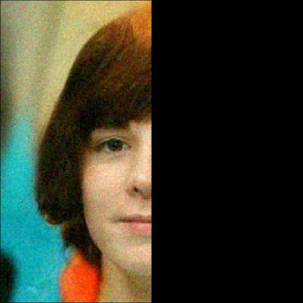
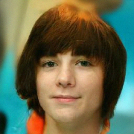
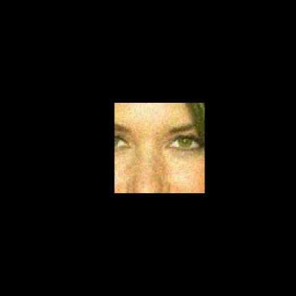
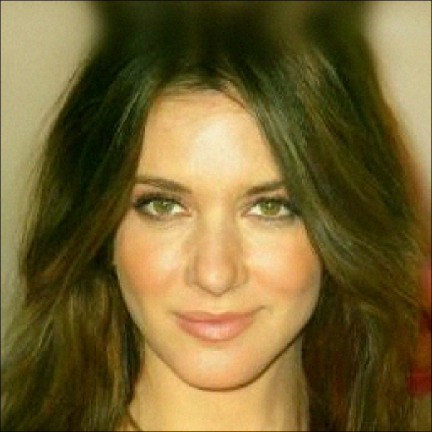
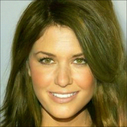
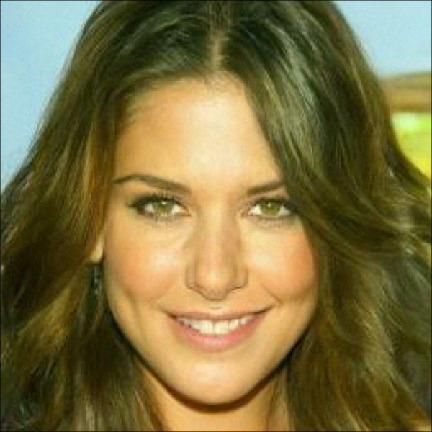
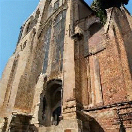
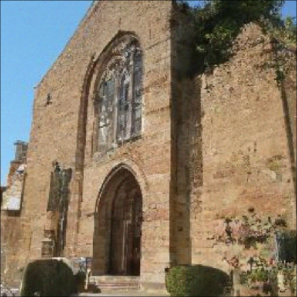
Figure 1: Posterior sampling using DCPS in the context of the image outpainting and super-resolution ($16\times$) Bayesian inverse problems.

In the present work, we consider Bayesian inverse problems based on DDM priors. In such models, posterior sampling is usually a challenge, because while sampling from the DDM is easy, evaluating the density is computationally difficult. Although approximations exist, the associated iterative sampling procedures can be computationally intensive and are sensitive to parameter choices; see, e.g., (Kawar et al., 2022). This motivates the development of methods for sampling from posterior distributions that arise from DDM priors (Kawar et al., 2022; Song et al., 2023a).

In this paper we propose the Divide-and-Conquer Posterior Sampler (DCPS) for denoising diffusion priors, a powerful sampling scheme for Bayesian inverse problems. This scheme targets backwards a sequence $(q_{k_{\ell}}^{y})_{\ell=0}^{L}$ of distributions forming a smooth path between the standard Gaussian distribution on $\mathbb{R}^{{d_{x}}}$ and the given posterior. These distributions correspond to pseudo-posteriors associated with a sequence of auxiliary linear inverse problems of increasing difficulty, ending at the original inverse problem. Given a sample from $q_{k_{\ell+1}}^{y}$, a draw from from $q_{k_{\ell}}^{y}$ is formed by a combination of Langevin iterates and the simulation of a non-homogeneous Markov chain. More precisely, we consider Feynman–Kac models (Del Moral, 2004) of moderate length $k_{\ell+1}-k_{\ell}\in\mathbb{N}^{*}$ that we sample approximately using a Gaussian variational inference scheme with initial distribution $q_{k_{\ell+1}}^{y,\ell}$ close to $q_{k_{\ell+1}}^{y}$. In turn, we sample $q_{k_{\ell+1}}^{y,\ell}$ using a Langevin algorithm starting from an approximate sample of $q_{k_{\ell+1}}^{y}$. The rationale behind our approach lies in the fact that the Gaussian approximation error can, as we show theoretically, be mitigated by shortening the length of the considered Feynman–Kac models (i.e., by increasing $L$). We illustrate the benefits of our methodology and its high reconstruction capability on synthetic data and various restoration tasks; see Figure 1 for curated reconstructions.

Notation.

For $(m,n)\in\mathbb{N}^{2}$ such that $m\leq n$, we let $\llbracket m,n\rrbracket\vcentcolon=\{m,\ldots,n\}$. We use $\phi(x;\mu,\Sigma)$ to denote the density at $x$ of a Gaussian distribution with mean $\mu$ and covariance matrix $\Sigma$. The $2$-Wasserstein distance between two probability measures $\mu$ and $\nu$ is defined as

$$W_{2}^{2}(\mu,\nu)=\inf_{\Pi\in\mathcal{C}(\mu,\nu)}\int\|x-y\|^{2}\,\Pi(\mathrm{d}(x,y))\,,$$

where $\mathcal{C}(\mu,\nu)$ is the set of all couplings of $\mu$ and $\nu$.

2 Denoising diffusion models

In this section we provide an overview of DDMs (Sohl-Dickstein et al., 2015; Song & Ermon, 2019; Ho et al., 2020). We assume that we have access to training samples from some unknown data distribution $p_{\tiny{\mbox{data}}}$ defined on $\mathbb{R}^{{d_{x}}}$. For every $t\in\llbracket 0,T\rrbracket$, define the distribution $q_{t}(x_{t})\vcentcolon=\int p_{\tiny{\mbox{data}}}(\mathrm{d}x_{0})\,q_{t|0}(x_{t}|x_{0})$, where

$$q_{t|0}(x_{t}|x_{0})\vcentcolon=\phi(x_{t};\sqrt{\alpha_{t}}x_{0},(1-\alpha_{t})I_{d_{x}})$$ (2.1)

and $(\alpha_{t})_{t\in\mathbb{N}}$ is a sequence that tends to zero as $t$ tends to infinity with $\alpha_{0}=1$ and $I_{d_{x}}$ is the ${d_{x}}\times{d_{x}}$ identity matrix. The density $q_{t}$ corresponds to the marginal at time $t$ of an auto-regressive process on $\mathbb{R}^{d_{x}}$ in the form

$$X_{t+1}=\sqrt{\alpha_{t+1}/\alpha_{t}}X_{t}+\sqrt{1-\alpha_{t+1}/\alpha_{t}}Z_{t+1}\,,$$ (2.2)

where $(Z_{t})_{t\in\mathbb{N}_{>0}}$ is a sequence of i.i.d. standard normal vectors and $X_{0}\sim p_{\tiny{\mbox{data}}}$. In order to define a generative model for $p_{\tiny{\mbox{data}}}$, DDMs leverage, for all $t\in\llbracket 0,T\rrbracket$, a parametric approximation $\hat{x}^{\theta}_{0|t}$ of the mapping $x_{t}\mapsto\int x_{0}\,q_{0|t}(\mathrm{d}x_{0}|x_{t})$, where $q_{0|t}(\mathrm{d}x_{0}|x_{t})\propto p_{\tiny{\mbox{data}}}(\mathrm{d}x_{0})\,q_{t|0}(x_{t}|x_{0})$ is the conditional distribution of $X_{0}$ given $X_{t}=x_{t}$. The denoiser $\hat{x}^{\theta}_{0|t}$ is typically defined in terms of a noise predictor neural network $\smash{\hat{\epsilon}^{\theta}_{t}}$ according to

$$\hat{x}^{\theta}_{0|t}(x_{t})\vcentcolon=\left(x_{t}-\sqrt{1-\alpha_{t}}\smash{\hat{\epsilon}^{\theta}_{t}}(x_{t})\right)\big{/}\sqrt{\alpha_{t}}\,.$$ (2.3)

By considering a single global neural network for all noise predictors, where $t$ is explicitly set as an input using positional encoding (Ho et al., 2020, Appendix C), DDMs learn a sequence $(\hat{x}^{\theta}_{0|t})_{t=1}^{T}$ of denoisers. This amounts to minimizing, using SGD, the objective

$$\sum_{t=1}^{T}w_{t}\mathbb{E}\left[\|\epsilon_{t}-\smash{\hat{\epsilon}^{\theta}_{t}}(\sqrt{\alpha_{t}}X_{0}+\sqrt{1-\alpha_{t}}\epsilon_{t})\|^{2}\right]$$ (2.4)

w.r.t. the neural network parameter $\theta$, where $(\epsilon_{t})_{t=1}^{T}$ are i.i.d. standard normal vectors and $(w_{t})_{t=1}^{T}$ are some nonnegative weights. We denote by $\theta^{\star}$ an estimator of the minimizer of the previous loss. Having access to $\theta^{\star}$, we can define a generative model for $p_{\tiny{\mbox{data}}}$ as described next.

While there are many ways to define such a model (Ho et al., 2020; Song et al., 2021c), we focus here on DDIMs (Song et al., 2021a). Let $(t_{k})_{k=0}^{n}$ be an increasing sequence of time instants in $\llbracket 0,T\rrbracket$ with $t_{0}=0$. We assume that $t_{n}$ is large enough so that $q_{t_{n}}$ (defined through (2.1)) is approximately multivariate standard normal. For convenience we assign the index $k$ to any quantity depending on $t_{k}$; e.g., we denote $p_{t_{k}}$ by $p_{k}$. For $k\in\llbracket 0,n-1\rrbracket$ and some hyperparameter $\eta\in[0,1]$ (whose design is discussed below), define $\smash{q}^{\eta}_{k|0,k+1}(\cdot|x_{0},x_{k+1})$ as the Gaussian distribution with mean

$$\mu_{k|0,k+1}(x_{0},x_{k+1})=\sqrt{\alpha_{k}}x_{0}\\ +\sqrt{1-\alpha_{k}-\sigma^{2}_{k|k+1}}\frac{x_{k+1}-\sqrt{\alpha_{k+1}}x_{0}}{\sqrt{1-\alpha_{k+1}}}$$ (2.5)

and diagonal covariance $\sigma^{2}_{k|k+1}I_{d_{x}}$, where, following Song et al. (2021a),

$$\sigma^{2}_{k|k+1}\vcentcolon=\eta^{2}(1-\alpha_{k})(1-\alpha_{k+1}/\alpha_{k})\big{/}(1-\alpha_{k+1})\,.$$

By convention we set $\smash{q}^{\eta}_{0|1}(\cdot|x_{1})\vcentcolon=\smash{q}_{0|1}(\cdot|x_{1})$. With this notation, we define the joint distribution

$$q^{\eta}_{0:n}(\mathrm{d}x_{0:n})=q_{n}(\mathrm{d}x_{n})\prod_{k=0}^{n-1}\smash{q}^{\eta}_{k|k+1}(\mathrm{d}x_{k}|x_{k+1})\,,$$ (2.6)

where

$$\smash{q}^{\eta}_{k|k+1}(\mathrm{d}x_{k}|x_{k+1})\\ \vcentcolon=\int\smash{q}^{\eta}_{k|0,k+1}(\mathrm{d}x_{k}|x_{0},x_{k+1})\,\smash{q}_{0|k+1}(\mathrm{d}x_{0}|x_{k+1})\,.$$ (2.7)

It holds that $q^{\eta}_{s}=q_{s}$ for all $s\in\llbracket 0,n\rrbracket$, where $q^{\eta}_{s}$ is the marginal of $q^{\eta}_{0:n}$ w.r.t. $x_{s}$ (see Song et al., 2021a, Lemma 1, Appendix B). Sampling from $q^{\eta}_{0}$ using $q^{\eta}_{0:n}$ yields exact draws from $p_{\tiny{\mbox{data}}}$; however, this is not feasible since the backward kernels (2.7) are intractable. Instead, Song et al. (2021c) consider the joint distribution

$$p^{\eta,\theta^{\star}}_{0:n}(\mathrm{d}x_{0:n})=p_{n}(\mathrm{d}x_{n})\prod_{k=0}^{n-1}\smash{p}^{\eta,\theta^{\star}}_{k|k+1}(\mathrm{d}x_{k}|x_{k+1})\,,$$ (2.8)

where $p_{n}$ is set to the multivariate standard normal distribution and for $k\in\llbracket 1,n-1\rrbracket$,

$$\smash{p}^{\eta,\theta^{\star}}_{k|k+1}(\mathrm{d}x_{k}|x_{k+1})\vcentcolon=\smash{q}^{\eta}_{k|0,k+1}(\mathrm{d}x_{k}|\hat{x}^{\theta^{\star}}_{0|k+1}(x_{k+1}),x_{k+1})$$ (2.9)

and $\smash{p}^{\eta,\theta^{\star}}_{0|1}(\cdot|x_{1})$ is set to the $\mathcal{N}(\hat{x}^{\theta^{\star}}_{0|1}(x_{1}),\sigma^{2}_{0|1}I_{d_{x}})$ distribution. We use the notation $\mu_{k|k+1}(x_{k+1})$ to denote the mean of the Gaussian distribution (2.9) and its definition follows immediately from (2.5). The transition kernel (2.9) can be viewed as an approximation of (2.7), where $x_{0}$ is replaced by $\hat{x}^{\theta^{\star}}_{0|k+1}(x_{k+1})$. In the following we drop the superscripts $\eta$ and $\theta^{\star}$ and simply write $p$ when referring to the generative model. In addition, we denote by $q_{k}$ the marginal of $p^{\eta,\theta^{\star}}_{0:n}$ (defined in (2.8)) w.r.t. $x_{k}$.

3 Posterior sampling with DDM prior

We now suppose that we have access to an observation $y\in\mathbb{R}^{d_{y}}$ of some random variable $Y$ defined through a linear model

$$Y=AX+\sigma_{y}Z\,,\quad X\sim p_{0},$$ (3.1)

a where $A\in\mathbb{R}^{{d_{y}}\times{d_{x}}}$ and $\sigma_{y}>0$ are known parameters and $Z$ is multivariate normal on $\mathbb{R}^{{d_{y}}}$. In the model above, $X$ is unobserved and $p_{0}$ is a prior distribution on $\mathbb{R}^{d_{x}}$. The main problem that we address is to sample from the posterior distribution of $X$—i.e., the conditional distribution of $X$ given $Y=y$—with distribution

$$p^{y}_{0}(\mathrm{d}x_{0})\vcentcolon=\smash{g^{y}_{0}}(x_{0})\,p_{0}(\mathrm{d}x_{0})/\mathcal{Z}\,,$$ (3.2)

where

$$\smash{g^{y}_{0}}(x_{0})\vcentcolon=\phi(y;Ax_{0},\sigma_{y}^{2}I_{d_{y}})$$ (3.3)

and $\mathcal{Z}\vcentcolon=\int\smash{g^{y}_{0}}(x_{0})\,p_{0}(\mathrm{d}x_{0})$ is the normalizing constant. We focus on the specific case where the prior $p_{0}$ is the marginal of (2.8) w.r.t. $x_{0}$, in which case the posterior (3.2) can be expressed as

$$p^{y}_{0}(\mathrm{d}x_{0})=\frac{1}{\mathcal{Z}}\int\smash{g^{y}_{0}}(x_{0})\prod_{k=0}^{n-1}\smash{p}_{k|k+1}(\mathrm{d}x_{k}|x_{k+1})\,p_{n}(\mathrm{d}x_{n})\,.$$

Thus, (3.2) can be interpreted as the marginal of a (time-reversed) Feynman–Kac (FK) model with a non-trivial potential only for $k=0$ (see Del Moral, 2004, for a comprehensive introduction to FK models). In this work, we twist, without modifying the law of the FK model, the backward transitions $\smash{p}_{k|k+1}$ by artificial potentials depending on the observation $y$, an idea that has already been explored in, e.g., rare event simulation (see, e.g., Cérou et al., 2012). More specifically, we introduce intermediate positive potentials $(g^{y}_{k})_{k=0}^{n}$, each being a function on $\mathbb{R}^{d_{x}}$, and write

$$p^{y}_{0}(\mathrm{d}x_{0})=\frac{1}{\mathcal{Z}}\int g^{y}_{n}(x_{n})\,p_{n}(\mathrm{d}x_{n})\\ \times\prod_{k=0}^{n-1}\frac{g^{y}_{k}(x_{k})}{g^{y}_{k+1}(x_{k+1})}\,\smash{p}_{k|k+1}(\mathrm{d}x_{k}|x_{k+1})\,.$$ (3.4)

This allows the posterior of interest to be expressed as the time-zero marginal of an FK model with initial law $p_{n}$, Markov transition kernels $(\smash{p}_{k|k+1})_{k=0}^{n-1}$ and potentials $g^{y}_{n}$ and $(x_{k},x_{k+1})\mapsto g^{y}_{k}(x_{k})/g^{y}_{k+1}(x_{k+1})$.

Related works.

Up to the knowledge of the authors, all recent works that aim to sample from the posterior (3.2) can be considered to operate using the FK representation (3.4), but with different choices of the auxiliary potentials (Chung et al., 2023; Song et al., 2023a; Zhang et al., 2023; Boys et al., 2023; Trippe et al., 2023; Wu et al., 2023). Define, for all $k$, the potentials

$$g^{y}_{k}(x_{k})\vcentcolon=\int\smash{g^{y}_{0}}(x_{0})\,\smash{p}_{0|k}(\mathrm{d}x_{0}|x_{k}),$$ (3.5)

which satisfy the recursion

$$g^{y}_{k+1}(x_{k+1})=\int g^{y}_{k}(x_{k})\,\smash{p}_{k|k+1}(\mathrm{d}x_{k}|x_{k+1})\,.$$

Consequently, in this case, the transition kernels

$$\smash{p}^{y}_{k|k+1}(\mathrm{d}x_{k}|x_{k+1})\vcentcolon=\frac{g^{y}_{k}(x_{k})}{g^{y}_{k+1}(x_{k+1})}\,\smash{p}_{k|k+1}(\mathrm{d}x_{k}|x_{k+1})$$ (3.6)

are Markov, and (3.4) can be rewritten as

$$p^{y}_{0}(\mathrm{d}x_{0})=\int p^{y}_{n}(\mathrm{d}x_{n})\prod_{k=0}^{n-1}\smash{p}^{y}_{k|k+1}(\mathrm{d}x_{k}|x_{k+1})\,.$$ (3.7)

Thus, the posterior $p^{y}_{0}$ becomes the time-zero marginal of a Markov model with transitions $(\smash{p}^{y}_{k|k+1})_{k=n-1}^{0}$. By this decomposition, sampling $X_{n}\sim p^{y}_{n}$ and then recursively $X_{k}^{y}\sim\smash{p}^{y}_{k|k+1}(\cdot|X_{k+1}^{y})$ for all $k\in\llbracket 0,n-1\rrbracket$ yields an exact sample from the posterior (3.2). In practice, however, neither the Markov kernels $\smash{p}^{y}_{k|k+1}$ nor the probability measure $p^{y}_{n}$ are tractable. In DPS (Chung et al., 2023), approximate samples from (3.6) are generated as follows. Given a sample $X^{y}_{k+1}$, an approximate sample $X^{y}_{k}$ from $\smash{p}^{y}_{k|k+1}(\cdot|X^{y}_{k+1})$ is obtained by first sampling $\tilde{X}^{y}_{k}\sim\smash{p}_{k|k+1}(\cdot|X^{y}_{k+1})$ and then setting

$$X^{y}_{k}=\tilde{X}^{y}_{k}+\zeta\nabla_{x_{k+1}}\log\smash{g^{y}_{0}}(\hat{x}_{0|k+1}(x_{k+1}))|_{x_{k+1}=X^{y}_{k+1}}\,.$$

where $\zeta>0$ is a tuning parameter. Here the gradient term is obtained by replacing, in (3.5), $\smash{p}_{0|k+1}(\cdot|x_{k+1})$ by a Dirac measure located at $\hat{x}_{0|k+1}(x_{k+1})$. As noted in (Song et al., 2023b; Cardoso et al., 2024; Boys et al., 2023) the DPS approximation has a significant bias and does not lead to an accurate approximation of the posterior even for the simplest examples; see also Section 5. Song et al. (2023a) improve the naive approximation of DPS by using a Gaussian approximation of $\smash{p}_{0|k}(\cdot|x_{k})$ with mean $\hat{x}_{0|k}(x_{k})$ and covariance matrix $\frac{1-\alpha_{k}}{2-\alpha_{k}}I_{d_{x}}$ in the case of variance preserving. This method makes it possible to mitigate part of the error associated with DPS, but still leads to a non-negligible residual bias; see (Boys et al., 2023). More recently, Boys et al. (2023) approximate the exact Gaussian projection of $\smash{p}_{0|k}(\cdot|x_{k})$, whose mean $\mu_{k}(x_{k})\vcentcolon=\int x_{0}\,\smash{p}_{0|k}(\mathrm{d}x_{0}|x_{k})$ and covariance matrix can be estimated using $\hat{x}_{0|k}(x_{k})$ and its Jacobian matrix.

Finally, FK models can be sampled using sequential Monte Carlo (SMC) methods, also known as particle filters; see (Del Moral, 2004; Chopin et al., 2020). These methods propagate sequentially weighted samples whose weighted empirical distributions target the flow of the FK marginal distributions. The efficiency of this approach depends crucially on the choice of the intermediate potentials $(g^{y}_{k})_{k=1}^{n}$. Different designs of these potentials are proposed in (Trippe et al., 2023; Wu et al., 2023; Cardoso et al., 2024; Dou & Song, 2024). However, the SMC method suffers from the curse of dimensionality and has difficulties when dealing with high-dimensional problems (Bickel et al., 2008). In Section 5 we show with a simple, low-dimensional example that DCPS exhibits a similar performance to SMC methods, which are known to be asymptotically exact as the number of particles tends to infinity.

4 The DCPS algorithm

Let $({k_{\ell}})_{\ell=0}^{L}$ be an increasing sequence in $\llbracket 0,n\rrbracket$, where ${k_{0}}=0$, ${k_{L}}=n$, and $L$ is typically much smaller than $n$, dividing $\llbracket 0,n\rrbracket$ into blocks $\llbracket{k_{\ell}},{k_{\ell+1}}-1\rrbracket$, $\ell\in\llbracket 0,L-1\rrbracket$. Our aim is now to define a sequence $(p^{y}_{{k_{\ell}}})_{\ell=0}^{L}$ of distributions guiding the sampler towards the target posterior $p^{y}_{0}=p^{y}_{{k_{0}}}$. These intermediate distributions are given by

$$p^{y}_{{k_{\ell}}}(\mathrm{d}x_{k_{\ell}})\vcentcolon=\smash{g^{y}_{{k_{\ell}}}}(x_{k_{\ell}})p_{{k_{\ell}}}(\mathrm{d}x_{k_{\ell}})\big{/}\mathcal{Z}^{y}_{{k_{\ell}}},$$ (4.1)

where $\mathcal{Z}^{y}_{k_{\ell}}\vcentcolon=\int\smash{g^{y}_{{k_{\ell}}}}(x_{k_{\ell}})p_{{k_{\ell}}}(\mathrm{d}x_{k_{\ell}})$ is the normalizing constant and $\smash{g^{y}_{{k_{\ell}}}}$ are potentials whose expressions are given below. On the contrary to (3.4), where the target posterior is expressed as the marginal of a single FK path measure of length $n$, we define $L$ FK models of each length ${k_{\ell+1}}-{k_{\ell}}$, $\ell\in\llbracket 0,L-1\rrbracket$. This will allow us to construct a recursive sampling scheme, where for each $\ell$, $p^{y}_{{k_{\ell}}}$ is targeted using samples from $p^{y}_{{k_{\ell+1}}}$. More precisely, we can write

$$p^{y}_{{k_{\ell}}}(\mathrm{d}x_{k_{\ell}})=\frac{1}{\mathcal{Z}^{y}_{{k_{\ell}}}}\int g^{y,\ell}_{{k_{\ell+1}}}(x_{k_{\ell+1}})\,p_{{k_{\ell+1}}}(\mathrm{d}x_{k_{\ell+1}})\\ \times\prod_{m={k_{\ell}}}^{{k_{\ell+1}}-1}\frac{g^{y,\ell}_{m}(x_{m})}{g^{y,\ell}_{m+1}(x_{m+1})}\,\smash{p}_{m|m+1}(\mathrm{d}x_{m}|x_{m+1})\,,$$ (4.2)

where $(g_{m}^{y,\ell})_{m={k_{\ell}}}^{{k_{\ell+1}}}$ are the potentials of model $\ell$ and $\smash{g^{y,\ell}_{{k_{\ell}}}}\vcentcolon=\smash{g^{y}_{{k_{\ell}}}}$. The design of the potentials, which is a cornerstone of our approach, is discussed next.

4.1 Definition of the potentials.

First, we start by defining the potential $\smash{g^{y}_{{k_{\ell}}}}$ as

$$\smash{g^{y}_{{k_{\ell}}}}(x_{k_{\ell}})=\phi(y_{k_{\ell}};Ax_{k_{\ell}},\sigma^{2}_{y,\ell}I_{d_{x}})\,,$$ (4.3)

where $\sigma_{y,\ell}>0$ is a user-specified parameter. To heuristically motivate this choice, we note that the corresponding distribution $p^{y}_{{k_{\ell}}}$, given by (4.2), is the posterior of $X_{k_{\ell}}$ given $Y_{k_{\ell}}=\sqrt{\alpha_{{k_{\ell}}}}y$ for the intermediate inverse problem

$$Y_{k_{\ell}}=AX_{k_{\ell}}+\sigma_{y,\ell}Z_{k_{\ell}}\,,$$ (4.4)

where $X_{k_{\ell}}\sim p_{{k_{\ell}}}$, $Z_{k_{\ell}}$ is ${d_{y}}$-dimensional independent standard Gaussian and $\sigma_{y,\ell}$ is a user-specified parameter. We shed light on the scaling of the observation $\sqrt{\alpha_{{k_{\ell}}}}$ with the next Lemma by assuming that the law of $X_{k_{\ell}}$ is that of $\sqrt{\alpha_{{k_{\ell}}}}X_{0}+\sqrt{1-\alpha_{{k_{\ell}}}}\varepsilon$ where $X_{0}\sim p_{0}$ and $\varepsilon\sim\mathcal{N}(0_{d_{x}},I_{d_{x}})$.

Lemma 4.1.

Let $\ell\in\llbracket 1,L\rrbracket$. Assume that $\sigma_{y,\ell}\geq\sqrt{\alpha_{{k_{\ell}}}}\sigma_{y}$ and that $X_{k_{\ell}}=\sqrt{\alpha_{{k_{\ell}}}}X_{0}+\sqrt{1-\alpha_{{k_{\ell}}}}\varepsilon_{\ell}$, where $X_{0}\sim p_{0}$, $\varepsilon\sim\mathcal{N}(0_{d_{x}},I_{d_{x}})$ and are independent. Then

$$Y_{k_{\ell}}\;\smash{\overset{\mathcal{L}}{=}}\;\sqrt{\alpha_{{k_{\ell}}}}\,Y+C\overline{Z}_{\ell}\,,$$ (4.5)

where $Y$ and $Y_{k_{\ell}}$ are defined in (3.1) and (4.4), respectively, $\overline{Z}_{\ell}\sim\mathcal{N}(0_{d_{y}},I_{d_{y}})$ is independent of $Y$ and

$$C\vcentcolon=\big{\{}(1-\alpha_{{k_{\ell}}})AA^{\intercal}+(\sigma^{2}_{y,\ell}-\alpha_{{k_{\ell}}}\sigma_{y}^{2})I_{d_{y}}\big{\}}^{1/2}\,.$$

Hence, given the realization $y$ of $Y$ we may sample uncorrelated observations $y_{k_{\ell}}$ using (4.5). We found in practice that simply setting and

$$y_{k_{\ell}}=\mathbb{E}[Y_{k_{\ell}}|Y=y]=\sqrt{\alpha_{{k_{\ell}}}}y\,,\quad\sigma_{y,\ell}=\sigma_{y}$$

where the expectation is under the conditional law defined by (4.5), yields the best empirical results.

We now turn to the design of the auxiliary potentials $g_{m}^{y,\ell}$ for $\ell\in\llbracket 0,L\rrbracket$ and $m\in\llbracket{k_{\ell}},{k_{\ell+1}}\rrbracket$. On the basis of definition (4.3) and similarly to (3.5), we may now define, for all $\ell$ and $m\in\llbracket{k_{\ell}}+1,{k_{\ell+1}}\rrbracket$,

$$g^{y,\ell}_{m}(x_{m})\vcentcolon=\int\smash{g^{y}_{{k_{\ell}}}}(x_{k_{\ell}})\,\smash{p}_{{k_{\ell}}|m}(\mathrm{d}x_{k_{\ell}}|x_{m})\,.$$ (4.6)

As $g^{y,\ell}_{m+1}(x_{m+1})=\int g^{y,\ell}_{m}(x_{m})\,\smash{p}_{m|m+1}(\mathrm{d}x_{m}|x_{m+1})$ by construction, the transition kernels

$$\smash{p}^{y,\ell}_{m|m+1}(\mathrm{d}x_{m}|x_{m+1})\vcentcolon=\frac{g^{y,\ell}_{m}(x_{m})\,\smash{p}_{m|m+1}(\mathrm{d}x_{m}|x_{m+1})}{g^{y,\ell}_{m+1}(x_{m+1})}\,,$$ (4.7)

are Markov, which implies, by (4.2), that $q^{y}_{{k_{\ell}}}$ is the law after ${k_{\ell+1}}-{k_{\ell}}$ iterations of an inhomogeneous Markov chain with kernels (4.7) and initial distribution

$$p^{y,\ell}_{{k_{\ell+1}}}(\mathrm{d}x_{k_{\ell+1}})=g^{y,\ell}_{{k_{\ell+1}}}(x_{k_{\ell+1}})\,p_{{k_{\ell+1}}}(\mathrm{d}x_{k_{\ell+1}})\big{/}\mathcal{Z}^{y}_{k_{\ell}}\,.$$ (4.8)

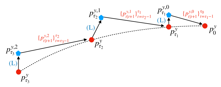
Figure 2: Illustration of DCPS  with $L=3$. Red dots refer to the distribution path (4.1) and $(\mathrm{L})$ denotes Langevin steps targeting $\smash{p^{y,\ell-1}_{{k_{\ell}}}}$ initialized at approximate samples from $\smash{p^{y}_{{k_{\ell}}}}$. Arrows starting from $\smash{p^{y,\ell-1}_{{k_{\ell}}}}$ and pointing to $p^{y}_{{k_{\ell-1}}}$ refer to ancestral sampling with transitions $\smash{(\smash{p}^{y,\ell-1}_{m|m+1})_{m={k_{\ell}}-1}^{{k_{\ell-1}}}}$.

Algorithm 1 Divide-and-Conquer Posterior Sampler (DCPS)

  Input: $y$, timesteps $({k_{\ell}})_{\ell=0}^{L}$, numbers $G$ and $K$ of gradient and Langevin steps, respectively. Initial sample $X^{y}_{k_{L+1}}\sim\mathcal{N}(0_{d_{x}},I_{d_{x}})$;

  for $\ell=L$ to $0$ do

     //Tamed Langevin steps to target (4.11); see (4.15).

     $\smash{X^{y,\ell}_{{k_{\ell+1}}}=\mathsf{TULA}(s^{\theta^{\star}}_{{k_{\ell+1}}}+\nabla_{x}\log\tilde{g}^{y,\ell}_{{k_{\ell+1}}},X^{y}_{k_{\ell+1}})}$;

     for $m={k_{\ell+1}}-1$ to ${k_{\ell}}$ do

        $\hat{\mu}^{0}_{m}=\mu_{m|m+1}(X^{y,\ell}_{m+1}),\,\hat{s}^{0}_{m}=\log\sigma^{2}_{{k_{\ell}}|m+1}\cdot\mathbf{1}_{d_{x}}$;

        //Optimization of the variational loss; see (4.13).

        $(\hat{\mu}_{m},\hat{s}_{m})=\mathsf{SGD}\big{(}\mathcal{L}_{t}(X^{y,\ell}_{m+1},\cdot);\hat{\mu}^{0}_{m},\hat{s}^{0}_{m}\big{)}$;

        $X^{y,\ell}_{m}=\hat{\mu}_{m}+(I_{d_{x}}\mathrm{e}^{\hat{s}_{m}/2})\varepsilon$, where $\varepsilon\sim\mathcal{N}(0_{d_{x}},I_{d_{x}})$;

     end for

     $X^{y}_{{k_{\ell}}}=X^{y,\ell}_{{k_{\ell}}}$;

  end for

We stress here that $q_{k_{\ell+1}}^{y,\ell}$ does not coincide with $q_{k_{\ell+1}}^{y}$; see Figure 2. Using the definitions above we may now formulate an ideal version of our algorithm, constructing as follows a Markov chain $(X^{y}_{{k_{\ell}}})_{\ell=L}^{0}$ backwards in time, with the law of $X^{y}_{k_{\ell}}$ being approximately $q^{y}_{{k_{\ell}}}$. Proceeding recursively, given $X^{y}_{k_{\ell+1}}$, we first use the unadjusted Langevin algorithm, initialized at $X^{y}_{{k_{\ell+1}}}$, to obtain an approximate sample $X^{y,\ell}_{k_{\ell+1}}$ from $p^{y,\ell}_{{k_{\ell+1}}}$; we then simulate a Markov chain with transition kernels $\smash{(\smash{p}^{y,\ell}_{m|m+1})_{m={k_{\ell+1}}-1}^{{k_{\ell}}}}$ starting at $X^{y,\ell}_{k_{\ell+1}}$, yielding an approximate draw from $q_{{k_{\ell}}}^{y}$. This procedure is repeated until the posterior $q_{k_{0}}^{y}=q_{0}^{y}$ of interest is reached; see Figure 2 for an illustration. Yet, in order to implement this sampling scheme, we need to approximate the intractable potentials $g^{y,\ell}_{m}$ and Markov kernels $\smash{p}^{y,\ell}_{m|m+1}$ by tractable counterparts $\tilde{g}^{y,\ell}_{m}$ and $\smash{\tilde{p}}^{y,\ell}_{m|m+1}$, respectively. The approximations that we will use share some similarities with those proposed by Chung et al. (2023); Song et al. (2023a); however, as we will see in the next paragraph, our framework allows the bias incurred by these approximations to be reduced and controlled by simply increasing the number $L$.

4.2 Approximate potentials.

In order to approximate the potential (4.6) for $\ell\in\llbracket 0,L\rrbracket$ and $m\in\llbracket{k_{\ell}}+1,{k_{\ell+1}}\rrbracket$, we leverage a Gaussian approximation $\smash{\tilde{p}}_{{k_{\ell}}|m}(\mathrm{d}x_{k_{\ell}}|x_{m})$ of the kernel $\smash{p}_{{k_{\ell}}|m}(\mathrm{d}x_{k_{\ell}}|x_{m})$ and estimate $g^{y,\ell}_{m}$ by the function $x_{m}\mapsto\int\smash{g^{y}_{{k_{\ell}}}}(x_{k_{\ell}})\,\smash{\tilde{p}}_{{k_{\ell}}|m}(\mathrm{d}x_{k_{\ell}}|x_{m})$. We consider the following Gaussian approximation which stems from DDIM:

$$\smash{\tilde{p}}_{{k_{\ell}}|m}(\mathrm{d}x_{k_{\ell}}|x_{m})\vcentcolon=\phi(\mathrm{d}x_{k_{\ell}};\mu_{{k_{\ell}}|m}(x_{m}),\sigma^{2}_{{k_{\ell}}|m}I_{d_{x}})\,,$$ (4.9)

where for $\ell\in\llbracket 1,L\rrbracket$,

$$\mu_{{k_{\ell}}|m}(x_{m})\vcentcolon=\sqrt{\alpha_{{k_{\ell}}}}\hat{x}_{0|m}(x_{m})\\ +\sqrt{1-\alpha_{{k_{\ell}}}-\sigma^{2}_{{k_{\ell}}|m}}\frac{x_{m}-\sqrt{\alpha_{{k_{\ell}}}}\hat{x}_{0|m}(x_{m})}{\sqrt{1-\alpha_{m}}}$$

and $\sigma^{2}_{{k_{\ell}}|m}\vcentcolon=\eta^{2}(1-\alpha_{{k_{\ell}}})(1-\alpha_{m}/\alpha_{{k_{\ell}}})\big{/}(1-\alpha_{m})$. For $\ell=0$, we set $\mu_{0|m}\vcentcolon=\hat{x}^{\theta^{\star}}_{0|m}$ and the variance $\sigma^{2}_{0|m}$ is a tuning parameter. In contrast to (Chung et al., 2023; Song et al., 2023a), we estimate expectations under $\smash{p}_{{k_{\ell}}|m}$ with $m\in\llbracket{k_{\ell}},{k_{\ell+1}}\rrbracket$ instead of expectations under $\smash{p}_{0|m}$ for $m\in\llbracket 0,n\rrbracket$. Denote by $\smash{q}^{\eta}_{{k_{\ell}}|0,m}(\mathrm{d}x_{k_{\ell}}|x_{0},x_{m})$ the conditional distribution under $q^{\eta}_{0:n}(\mathrm{d}x_{0:n})$ of $x_{k_{\ell}}$ given $x_{0}$ and $x_{m}$. We show in the Section B.1 that this corresponds to a Gaussian distribution when $\eta=1$. In the next proposition, we show, under appropriate conditions, that given a Gaussian approximation $\smash{\hat{p}}_{0|m}(\mathrm{d}x_{0}|x_{m})$ of $\smash{p}_{0|m}(\mathrm{d}x_{0}|x_{m})$, the approximation error of the kernel

$$\smash{\hat{p}}_{{k_{\ell}}|m}(\mathrm{d}x_{k_{\ell}}|x_{m})\vcentcolon=\int\smash{q}^{\eta}_{{k_{\ell}}|0,m}(\mathrm{d}x_{k_{\ell}}|x_{0},x_{m})\smash{\hat{p}}_{0|m}(\mathrm{d}x_{0}|x_{m})$$

w.r.t $\smash{p}_{{k_{\ell}}|m}(\mathrm{d}x_{k_{\ell}}|x_{m})$ is always smaller than that of $\smash{\hat{p}}_{0|m}$ w.r.t. $\smash{p}_{0|m}$. Furthermore, the approximation error decreases as $m$ tends to ${k_{\ell}}$.

Proposition 4.2.

Assume that $\eta=1$ and that for all $j\in\llbracket 0,n-1\rrbracket$, $\smash{p}_{j|j+1}(\mathrm{d}x_{j}|x_{j+1})=\smash{q}^{\eta}_{j|j+1}(\mathrm{d}x_{j}|x_{j+1})$ for all $x_{j+1}\in\mathbb{R}^{{d_{x}}}$. Then for all $\ell\in\llbracket 0,L\rrbracket$, $m\in\llbracket{k_{\ell}}+1,{k_{\ell+1}}\rrbracket$, and $x_{m}\in\mathbb{R}^{d_{x}}$,

$$W_{2}(\smash{\hat{p}}_{{k_{\ell}}|m}(\cdot|x_{m}),\smash{p}_{{k_{\ell}}|m}(\cdot|x_{m}))\\ \leq\frac{\sqrt{\alpha_{{k_{\ell}}}}(1-\alpha_{m}/\alpha_{{k_{\ell}}})}{(1-\alpha_{m})}W_{2}(\smash{\hat{p}}_{0|m}(\cdot|x_{m}),\smash{p}_{0|m}(\cdot|x_{m}))\,.$$

The proof is postponed to Section B.1. We can improve all the approximations proposed in the literature by choosing $\smash{\tilde{p}}_{{k_{\ell}}|m}$ adequately. For instance, under the stated assumptions, if $\smash{\hat{p}}_{0|m}(\mathrm{d}x_{0}|x_{m})$ is the DPS approximation, i.e., $\smash{\hat{p}}_{0|m}(\mathrm{d}x_{0}|x_{m})=\delta_{\hat{x}^{\theta^{\star}}_{0|m}(x_{m})}(\mathrm{d}x_{0})$, then $\smash{\hat{p}}_{{k_{\ell}}|m}(x_{k_{\ell}}|x_{m})=\smash{\tilde{p}}_{{k_{\ell}}|m}(\mathrm{d}x_{k_{\ell}}|x_{m})$ as defined in (4.9), and we hence improve upon DPS in terms of approximation error. We may also consider the Gaussian approximation of (Song et al., 2023a) and define $\smash{\tilde{p}}_{{k_{\ell}}|m}(\mathrm{d}x_{k_{\ell}}|x_{m})$ accordingly.

Using (4.3) as potentials, we then, using (Bishop, 2006, Eq. 2.115), take, for $m\in\llbracket{k_{\ell}}+1,{k_{\ell+1}}\rrbracket$,

$$\tilde{g}^{y,\ell}_{m}(x_{m}) \vcentcolon=\int g^{y}_{{k_{\ell}}}(x_{k_{\ell}})\smash{\tilde{p}}_{{k_{\ell}}|m}(\mathrm{d}x_{k_{\ell}}|x_{m})$$ (4.10)

$$=\phi(y_{k_{\ell}};A\mu_{{k_{\ell}}|m}(x_{m}),\sigma^{2}_{{k_{\ell}}|m}AA^{\intercal}+\sigma^{2}_{y,\ell}I_{d_{y}})$$

as an approximation of $\smash{g^{y,\ell}_{m}}$. For $m={k_{\ell}}$ we set $\tilde{g}^{y,\ell}_{{k_{\ell}}}=\smash{g^{y}_{{k_{\ell}}}}$. With these approximations we now define,

$$\tilde{p}^{y,\ell}_{{k_{\ell+1}}}(\mathrm{d}x_{k_{\ell}})\propto\tilde{g}^{y,\ell}_{{k_{\ell+1}}}(x_{k_{\ell+1}})\,p_{{k_{\ell+1}}}(\mathrm{d}x_{k_{\ell+1}})$$ (4.11)

and

$$\textstyle\smash{\tilde{p}}^{y,\ell}_{m|m+1}(\mathrm{d}x_{m}|x_{m+1})\propto\tilde{g}^{y,\ell}_{m}(x_{m})\,\smash{p}_{m|m+1}(\mathrm{d}x_{m}|x_{m+1})\,,$$ (4.12)

which act as replacements of $p^{y,\ell}_{{k_{\ell+1}}}$ and $\smash{p}^{y,\ell}_{m|m+1}$, respectively, in the next section.

4.3 Local variational approximation.

We now turn to the variational approximation of the backward transition kernels $\smash{\tilde{p}}^{y,\ell}_{m|m+1}$ in (4.12). For $m\in\llbracket{k_{\ell}},{k_{\ell+1}}\rrbracket$ and a fixed $x_{m+1}$ we seek a mean-field Gaussian variational approximation of $\smash{\tilde{p}}^{y,\ell}_{m|m+1}(\cdot|x_{m+1})$ by solving

$$\operatorname*{argmin}_{r^{y,\ell}_{m|m+1}(\cdot|x_{m+1})\in\mathcal{G}_{D}}\mathsf{KL}(r^{y,\ell}_{m|m+1}(\cdot|x_{m+1})\parallel\smash{\tilde{p}}^{y,\ell}_{m|m+1}(\cdot|x_{m+1}))\,,$$

where $\mathcal{G}_{\mathrm{D}}\vcentcolon=\{\mathcal{N}(\mu,I_{d_{x}}\sigma):\mu\in\mathbb{R}^{{d_{x}}},\sigma\in\mathbb{R}^{{d_{x}}}_{>0}\}$. The previous KL objective, which we denote by $\mathsf{KL}^{y,\ell}_{m}(x_{m+1})$, can be expanded as follows (up to a normalizing constant),

$$\mathsf{KL}^{y,\ell}_{m}(x_{m+1})=-\int\log\tilde{g}^{y,\ell}_{m}(x_{m})\,r^{y,\ell}_{m|m+1}(\mathrm{d}x_{m}|x_{m+1})\\ +\mathsf{KL}(r^{y,\ell}_{m|m+1}(\cdot|x_{m+1})\parallel\smash{p}_{m|m+1}(\cdot|x_{m+1}))\,,$$ (4.13)

where the second term on the r.h.s. can be computed exactly. Letting $r^{y,\ell}_{m|m+1}(\cdot|x_{m+1})$ be the $\mathcal{N}(\hat{\mu}_{m},I_{d_{x}}\mathrm{e}^{\hat{s}_{m}})$ distribution, where $(\hat{\mu}_{m},\hat{s}_{m})\in(\mathbb{R}^{d_{x}})^{2}$ are the variational approximation parameters and $\mathrm{e}^{\hat{s}_{m}}\vcentcolon=(\mathrm{e}^{\hat{s}_{m,1}},\dotsc,\mathrm{e}^{\hat{s}_{m,{d_{x}}}})^{\intercal}$, the optimization objective becomes

$$\mathcal{L}_{m}(x_{m+1};\hat{\mu}_{m},\hat{s}_{m})\vcentcolon=-\mathbb{E}\big{[}\log\tilde{g}^{y,\ell}_{m}(\hat{\mu}_{m}+(I_{d_{x}}\mathrm{e}^{\hat{s}_{m}/2})Z)\big{]}$$

$$+\frac{\|\hat{\mu}_{m}-\mu_{m|m+1}(x_{m+1})\|^{2}}{2\sigma^{2}_{m|m+1}}-\frac{1}{2}\sum_{i=1}^{d_{x}}(\hat{s}_{m,i}-\frac{\mathrm{e}^{\hat{s}_{m,i}}}{\sigma^{2}_{m|m+1}})\,,$$

where $Z$ is ${d_{x}}$-dimensional standard normal. Here we have reparameterized the expectation in $\mathsf{KL}^{y,\ell}_{m}(x_{m+1})$ so that it is amenable to stochastic gradient optimization (Kingma & Welling, 2013), and used the closed-form expression (up to some constants independent of $\hat{\mu}_{m},s_{m}$) of the KL divergence between two multivariate Gaussians. Finally, we optimize the previous objective using a few steps of SGD, where we estimate the expectation of the log integrated potential by drawing a single noise vector $Z$.

The previous optimization objective involves evaluating $\tilde{g}^{y,\ell}_{m}$ and requires inverting the matrix $\sigma^{2}_{{k_{\ell}}|m}AA^{\intercal}+\sigma^{2}_{y,\ell}I_{d_{y}}$ at each step $m$. This computational overhead can be mitigated by initially computing the eigendecomposition of the matrix $AA^{\intercal}$. The covariance matrix can then be effectively inverted at each step. In the cases where the eigendecomposition is expensive to compute, we instead recommend using the biased Monte Carlo estimate $\log\tilde{g}^{y,\ell}_{m}(x_{m})\approx\log g^{y}_{{k_{\ell}}}(\mu_{{k_{\ell}}|m}(x_{m})+\sigma_{{k_{\ell}}|m}\tilde{Z})$. One may also minimize an upper-bound on the KL divergence by considering an implicit Gaussian parameterization for $r^{y,\ell}_{m|m+1}(\cdot|x_{m+1})$ as we detail in Section A.1. Finally, we insist that we only perform a few gradient steps to optimize the previous loss. In our experiments we perform only two gradient steps at each step $m$ and so our algorithm’s runtime is comparable to that of its competitors.

4.4 Sampling the initial distribution.

Finally, to initialize the Markov chain with transition kernels $(r^{y,\ell}_{m|m+1})_{m={k_{\ell+1}}-1}^{{k_{\ell}}}$ we require an initial approximate sample from $\tilde{p}^{y,\ell}_{{k_{\ell+1}}}$ in (4.11). For this step we propose to use a discretization of the Langevin dynamics (Roberts & Tweedie, ) or an approximate Gibbs sampler (Gelfand, 2000). The latter allows us to frame the RePaint algorithm (Lugmayr et al., 2022) as a special case of our framework; see Section 4.5. We detail the Langevin approach herebelow and defer the approximate Gibbs sampler to Section A.2.

As the marginal distributions $(p_{k})_{k=0}^{n}$ approximate the marginals $(q_{k})_{k=0}^{n}$, we may, for each $k\in\llbracket 0,n\rrbracket$, use the score

$$\textstyle s^{\theta^{\star}}_{k}(x_{k})=-(x_{k}-\sqrt{\alpha_{k}}\hat{x}^{\theta^{\star}}_{0|k}(x_{k}))/(1-\alpha_{k})$$ (4.14)

as a substitute for $\nabla\log p_{k}$; see, e.g., (Dhariwal & Nichol, 2021, Section 4.2). As a result, we sample from $p^{y,\ell}_{{k_{\ell+1}}}$ by running $M$ steps of the Tamed Unadjusted Langevin scheme (Brosse et al., 2019)

$$X_{j+1}=X_{j}+\gamma G^{y,\ell}_{\gamma}(X_{j})+\sqrt{2\gamma}Z_{j}\,,\quad X_{0}=X^{y}_{k_{\ell+1}}\,,$$ (4.15)

where $(Z_{j})_{j=0}^{M-1}$ are i.i.d. ${d_{x}}$-dimensional standard normal, $X^{y}_{k_{\ell+1}}$ is an approximate sample from $q^{y}_{{k_{\ell+1}}}$, and for all $x\in\mathbb{R}^{d_{x}}$ and $\gamma>0$,

$$G^{y,\ell}_{\gamma}(x)\vcentcolon=\frac{\nabla\log\tilde{g}^{y,\ell}_{{k_{\ell+1}}}(x)+s^{\theta^{\star}}_{{k_{\ell+1}}}(x)}{1+\gamma\|\nabla\log\tilde{g}^{y,\ell}_{{k_{\ell+1}}}(x)+s^{\theta^{\star}}_{{k_{\ell+1}}}(x)\|}\,.$$

We then set $X^{y,\ell}_{{k_{\ell+1}}}\vcentcolon=X_{M}$. See Algorithm 2 for a complete version of our algorithm.

4.5 Related methods

In this section we discuss existing methods that are close to ours in terms of our choice of sequence of distributions (4.1) and potentials (4.3). Setting $L=n$ (and hence $k_{\ell}=\ell$) and using a Gibbs sampler to sample from the consecutive distributions allows us to recover a generalization of the RePaint algorithm (Lugmayr et al., 2022). Indeed, note that (4.1) is the marginal of the joint distribution

$$p^{y}_{\ell,\ell+1}(\mathrm{d}(x_{\ell},x_{\ell+1}))$$ (4.16)

$$\hskip 8.5359pt\vcentcolon=\smash{g^{y}_{\ell}}(x_{\ell})\smash{p}_{\ell|\ell+1}(\mathrm{d}x_{\ell}|x_{\ell+1})p_{\ell+1}(\mathrm{d}x_{\ell+1})\big{/}\mathcal{Z}^{y}_{\ell,\ell+1}\,,$$

where $\mathcal{Z}^{y}_{\ell,\ell+1}\vcentcolon=\int\smash{g^{y}_{\ell}}(x_{\ell})\smash{p}_{\ell|\ell+1}(\mathrm{d}x_{\ell}|x_{\ell+1})p_{\ell+1}(\mathrm{d}x_{\ell+1})$. Hence, we can draw approximate samples from $p^{y}_{\ell}$ with a Gibbs sampler targeting $p^{y}_{\ell,\ell+1}$. A Gibbs sampler (Gelfand, 2000) constructs a Markov chain $(X^{y}_{\ell,k},X^{y}_{\ell+1,k})_{k}$ targeting $p^{y}_{\ell,\ell+1}$ by alternating the sampling of the two conditional distributions of (4.16)

$$\smash{p}^{y}_{\ell|\ell+1}(\mathrm{d}x_{\ell}|x_{\ell+1}) \propto\smash{g^{y}_{\ell}}(x_{\ell})\smash{p}_{\ell|\ell+1}(\mathrm{d}x_{\ell}|x_{\ell+1})\,,$$

$$\smash{p}^{y}_{\ell+1|\ell}(\mathrm{d}x_{\ell+1}|x_{\ell}) \propto\smash{p}_{\ell|\ell+1}(x_{\ell}|x_{\ell+1})p_{\ell+1}(\mathrm{d}x_{\ell+1})\,.$$

Given $(X^{y}_{\ell,k},X^{y}_{\ell+1,k})$, $(X^{y}_{\ell,k+1},X^{y}_{\ell+1,k+1})$ is obtained by drawing $X^{y}_{\ell,k+1}$ from $\smash{p}^{y}_{\ell|\ell+1}(\cdot|X^{y}_{\ell+1,k})$ and $X^{y}_{\ell+1,k+1}$ from $\smash{p}^{y}_{\ell+1|\ell}(\cdot|X^{y}_{\ell,k+1})$. With the choice of potential (4.3), $\smash{p}^{y}_{\ell|\ell+1}(\cdot|X^{y}_{\ell+1,k})$ can be sampled exactly. The second conditional $\smash{p}^{y}_{\ell+1|\ell}(\mathrm{d}x_{\ell+1}|x_{\ell})$ cannot however and Lugmayr et al. (2022) approximate it with the forward kernel (2.2). This is exact and not an approximation when the backward kernel is learned perfectly. The Gibbs sampler is thus not exact in practice. As we show in Section A.2, RePaint, which is specific tonoiseless inverse problem ($\sigma_{y}=0$ in (3.1)), is recovered exactly by setting for all $\ell\in\llbracket 0,n\rrbracket$ in (4.3), $\sigma_{y,\ell}=0$ and using $y_{\ell}=\sqrt{\alpha_{\ell}}\,y+\sqrt{1-\alpha_{\ell}}Z_{\ell}$ where $Z_{\ell}$ are i.i.d. standard Gaussian samples. The algorithm proposed in Cardoso et al. (2024) also operates using the sequence (4.1), potentials (4.3) and with $L=n$. They obtain empirical approximations of the successive distributions using a SMC sampler. For the noiseless case, they use the potentials (4.3) with observations $y_{\ell}=\sqrt{\alpha_{\ell}}\,y$ similar to us but with standard deviation $\sigma_{y,\ell}=\sqrt{1-\alpha_{\ell}}$. Dou & Song (2024) develop a similar SMC methodology with $\sigma_{y,\ell}=\sqrt{\alpha_{\ell}}\sigma_{y}$ and the observations are sampled recursively backwards according to $y_{\ell}=u_{\ell+1}y+v_{\ell+1}y_{\ell+1}+w_{\ell+1}AZ_{\ell+1}$ where $(u_{\ell},v_{\ell},w_{\ell})_{\ell}$ are DDIM coefficients.

5 Experiments

In this section we demonstrate the performance of our algorithm and compare it with DPS (Chung et al., 2023), DDRM (Kawar et al., 2022), and MCGDiff  (Cardoso et al., 2024). A prerequisite for quantitative evaluation in ill-posed Bayesian inverse problems is to have access to samples from the posterior distribution. Hence, we first consider a linear inverse problem with a Gaussian mixture (GM) prior. In this case, exact samples from the posterior are available. Furthermore, the global minimizer of the objective (2.4) is available in a closed form; see Section C.1 for more details. We then apply our algorithm to the super-resolution (SR), inpainting, outpainting, and colorization problems on three datasets: the CelebA-HQ (256), LSUN-Church (256), and LSUN-Bedroom (256) (Ho et al., 2020). We use publicly available pre-trained score models that can be found on Hugging Face. We provide the experimental details in Section C.2.

5.1 Gaussian mixture.

For the GM prior, we reproduce the experiment of (Cardoso et al., 2024). We consider a mixture of $P=25$ components with fixed means $(\mathbf{m}_{i})_{i=1}^{P}$ and unit covariances in ${d_{x}}=10$ and ${d_{x}}=100$ dimensions. We repeat the experiment with 20 different seeds. For each seed, we generate some mixture weights $(w_{i})_{i=1}^{P}$ and a measurement model $(y,A,\sigma_{y})$, where ${d_{y}}=1$. The posterior is a Gaussian mixture whose means, covariance matrices, and weights are given by $(\tilde{\mathbf{m}}_{i})_{i=1}^{P}$, $(\tilde{\Sigma}_{i}I_{{d_{x}}})_{i=1}^{P}$, and $(\tilde{w}_{i})_{i=1}^{P}$, respectively. Details can be found in Section C.1. Then, for each pair of prior distribution and measurement model, we draw $N_{s}=2000$ samples using each algorithm and compare them with $N_{s}$ samples from the true posterior distribution, using the Sliced Wasserstein distance. We also compute MLE estimates $(\hat{w}_{i})_{i=1}^{P}$ of the weights using the samples drawn from the posteriors. We compare these estimates with the weights $(w_{i})_{i=1}^{P}$ by computing and averaging, over the 20 seeds, the quantity $\Delta w\vcentcolon=(\sum_{i=1}^{P}|w_{i}-\hat{w}_{i}|^{2})^{1/2}$. The results are given in Table 1. We test two configurations with $L=4$ intermediate posteriors, $G=2$ gradient steps, and $50$ and $500$ steps each of the unadjusted Langevin; see Algorithm 1. We denote these configurations by $\mathrm{{\sc{DCPS}}}_{50}$ and $\mathrm{{\sc{DCPS}}}_{500}$, respectively, in Table 1. We use 400 DDIM steps for each algorithm.

	${d_{x}}=10,\,{d_{y}}=1$			${d_{x}}=100,\,{d_{y}}=1$
	SW	$\Delta w$		SW	$\Delta w$
MCGDiff	$2.25/2.69\pm 2.07$	$0.32\pm 0.20$		$2.72/3.13\pm 1.76$	$0.42\pm 0.19$
DPS	$3.12/5.64\pm 8.45$	$0.20\pm 0.12$		$4.29/4.93\pm 4.85$	$0.35\pm 0.25$
DDRM	$2.66/3.06\pm 1.90$	$0.36\pm 0.16$		$5.97/6.26\pm 2.33$	$0.52\pm 0.19$
$\mathrm{{\sc{DCPS}}}_{50}$	$1.95/2.70\pm 2.28$	$0.17\pm 0.25$		$4.40/4.72\pm 2.18$	$0.44\pm 0.16$
$\mathrm{{\sc{DCPS}}}_{500}$	$1.26/2.59\pm 2.83$	$0.13\pm 0.30$		$2.81/3.22\pm 2.21$	$0.32\pm 0.18$

Table 1: Results for the Gaussian mixture experiment. Results for the SW distance are shown in median/mean ± standard deviation format.

5.2 Imaging experiment.

For all tasks and datasets we use the same parameters for our algorithm and hence do not perform any task-specific or data-specific tuning. We use $L=4$, $G=2$, and $5$ Langevin steps. We use 400 DDIM steps for all algorithms with $\eta=1$. For DPS we have tried using the step-sizes provided in the original paper but found that these did not work on the datasets we consider, which are different from those in the paper in question. We tuned DPS the parameters on each task and each dataset; however, none of the parameters we found worked consistently on all the experiments.

The posterior of the examples we consider next, besides SR $4\times$, are highly multimodal, and we thus believe that comparisons with groundtruth images through the LPIPS provide meaningless results. Metrics such as the Fréchet Inception Distance (FID) are also not suited for the evaluation of Bayesian restoration methods. Notably, an algorithm that fails to sample from the posterior and instead generates samples from the prior may still achieve a favorable FID score. We thus refrain from using these and rely on qualitative evaluation only. We use the same initialization for all the algorithms and draw, for each task and algorithm, $5$ i.i.d. samples. We display the first sample for each method herebelow, see Figure 3, Figure 5, and Figure 4. The remaining samples are shown in the appendix.

We note that although DPS can yield competitive reconstructions in several scenarios, there are numerous instances where it struggles to maintain consistency with the observed portions of the image. This issue is exemplified in Figure 5 and Figure 4 and further in Section C.2. Notably, similar challenges have been reported in recent studies involving GM experiments, as evidenced by Cardoso et al. (2024, Section 3) and Boys et al. (2023, Section 6.1). The observed phenomenon suggests that DPS might assign disproportionate weights to modes with minimal posterior weights, leading to the generation of samples that exhibit only partial consistency with the observed segments of the image. In our examination of DDRM, we consistently find that it tends to produce images that are coherent yet lack sharpness. Additionally, all generated samples exhibit striking similarity, suggesting a probable collapse of the resulting posterior approximation onto a single mode. On the other hand, DCPS produces sharp, coherent, and diversified reconstructions without any task or data-specific tuning.

$y$	DCPS	DPS	DDRM

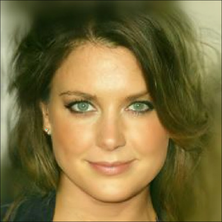
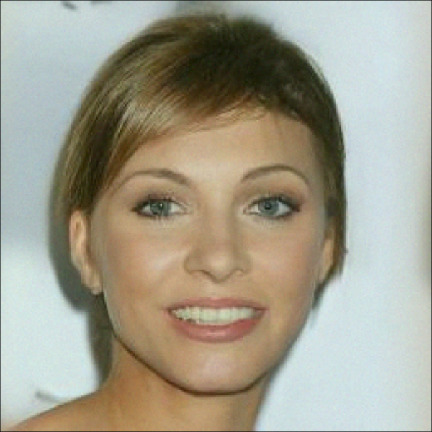
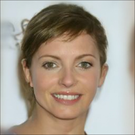
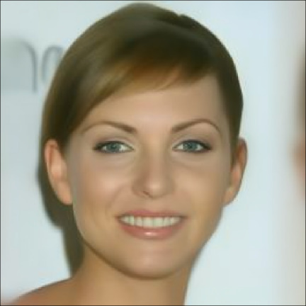
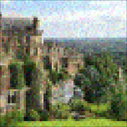
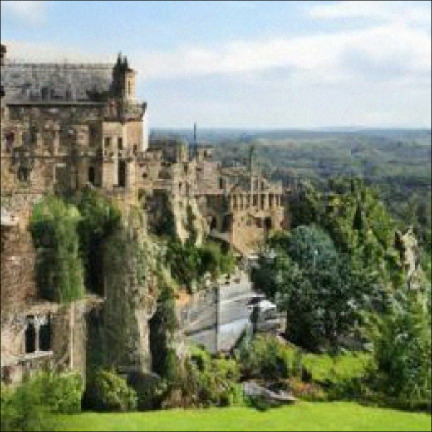
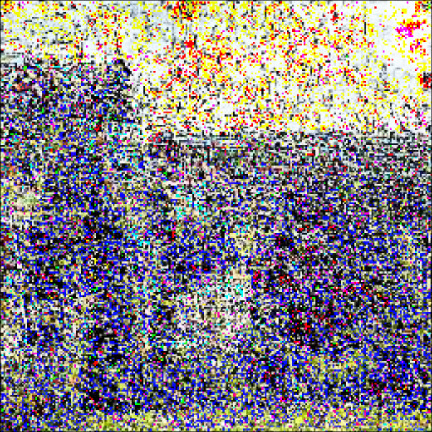
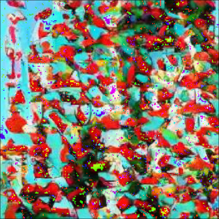
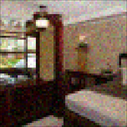
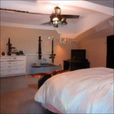
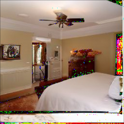
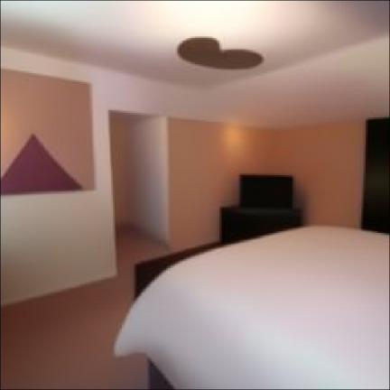
Figure 3: Super-resolution ($4\times$ & $16\times$) experiment. The remaining samples are displayed in Section C.2.1

$y$	DCPS	DPS	DDRM

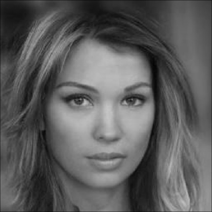
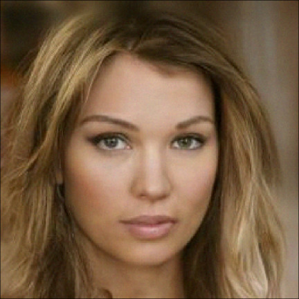
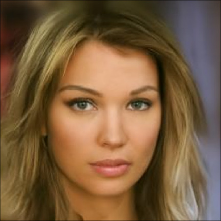
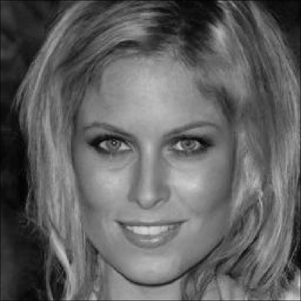
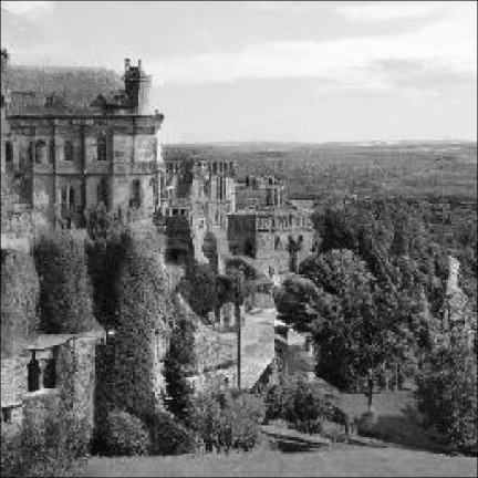
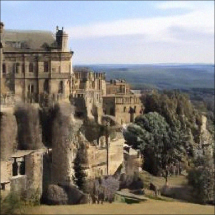
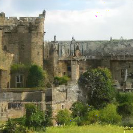
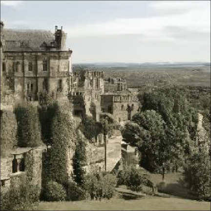
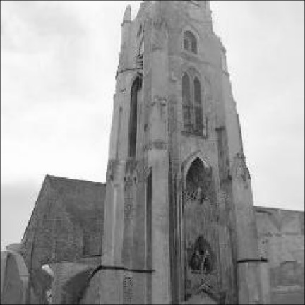
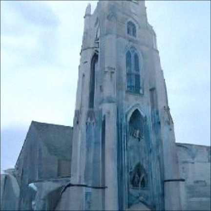
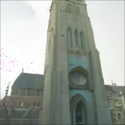
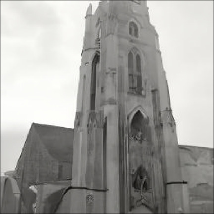
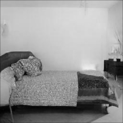
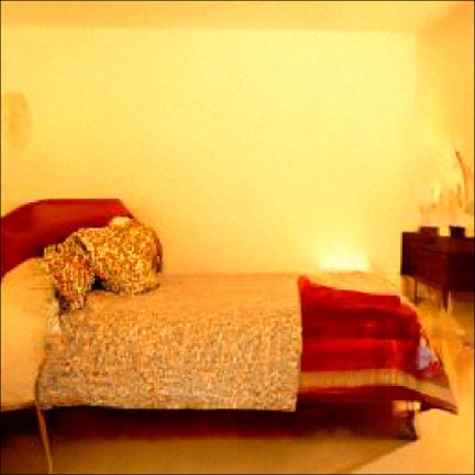
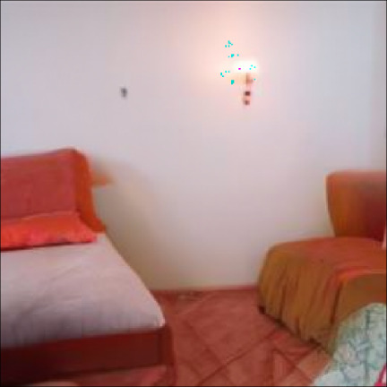
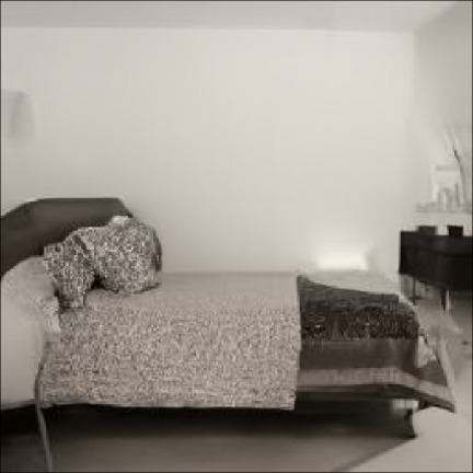
Figure 4: Colorization experiments. The remaining samples are displayed in Section C.2.3.

$y$	DCPS	DPS	DDRM

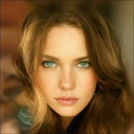
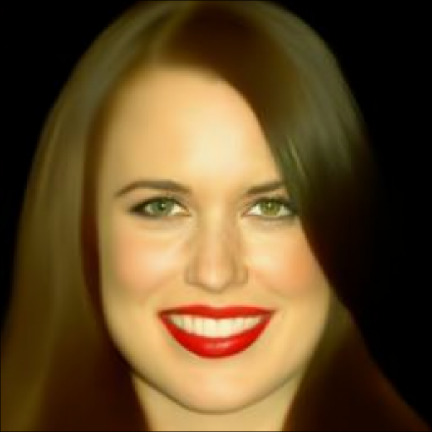
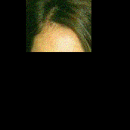
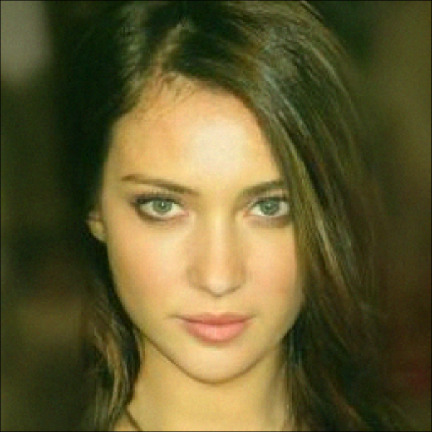
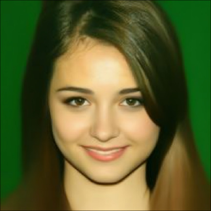
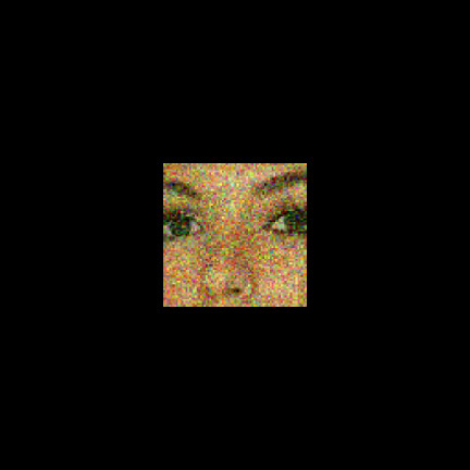
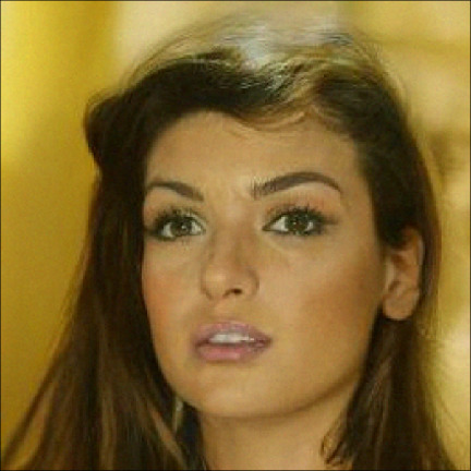
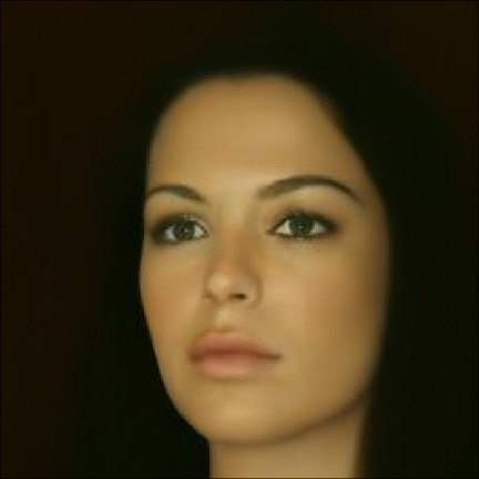
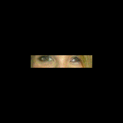
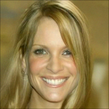
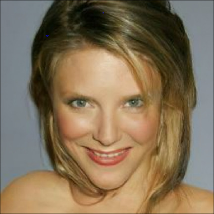
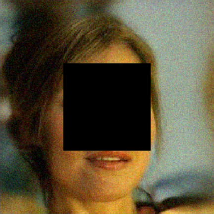
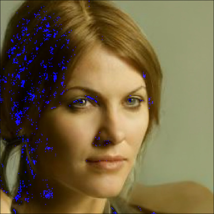
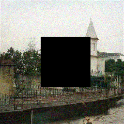
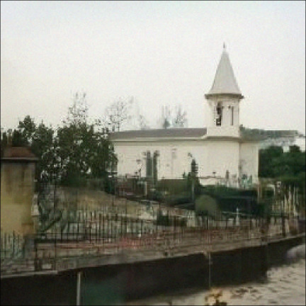
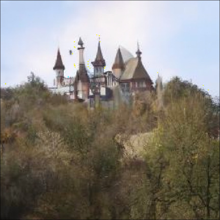
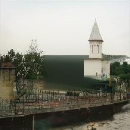
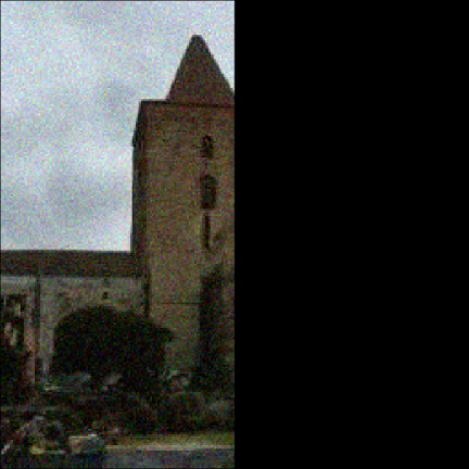
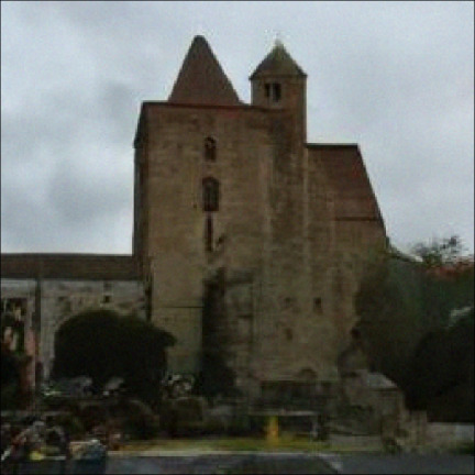
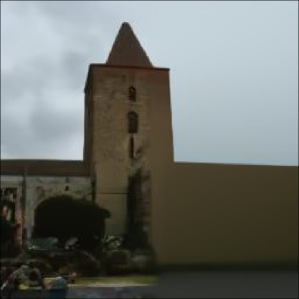
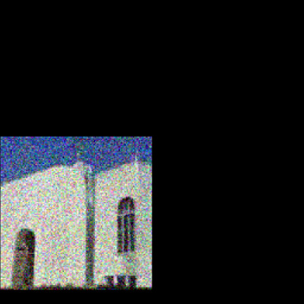
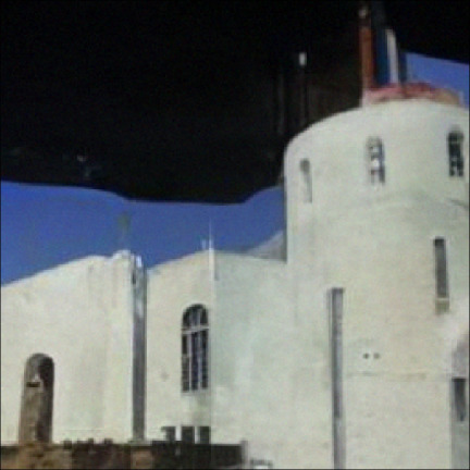
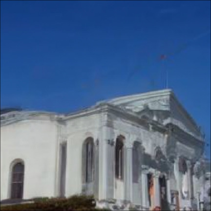
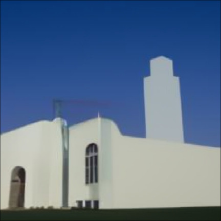
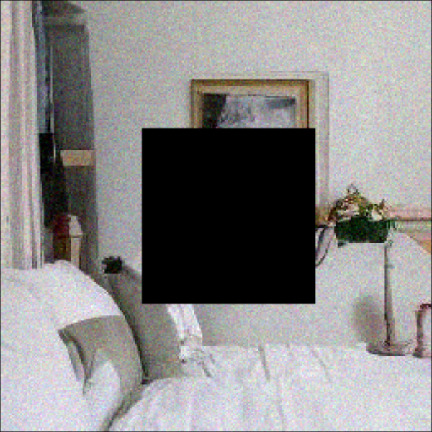
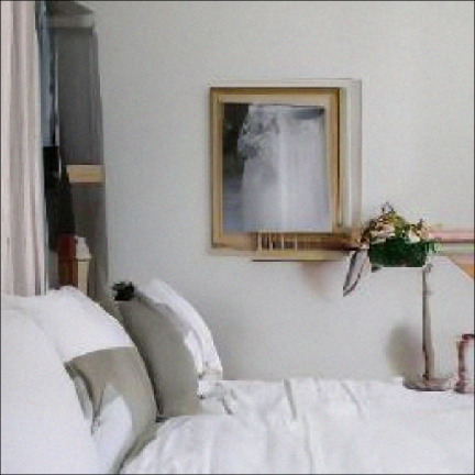
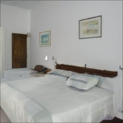
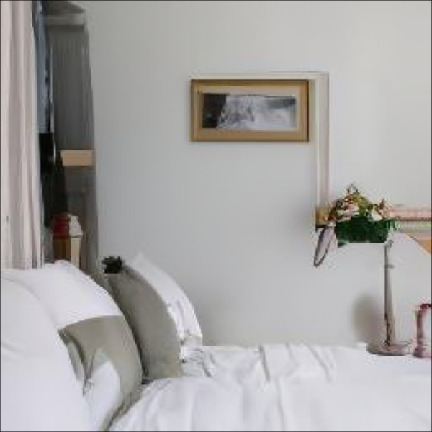
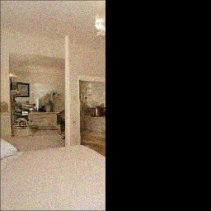
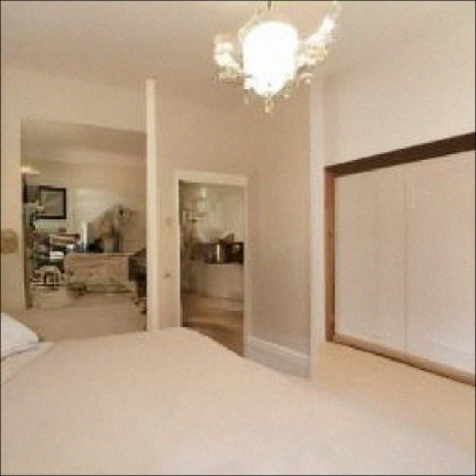
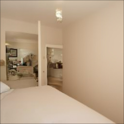
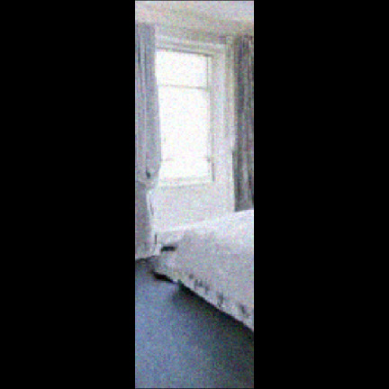
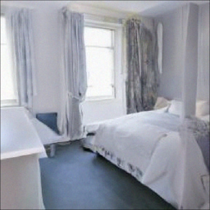
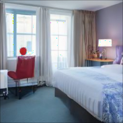
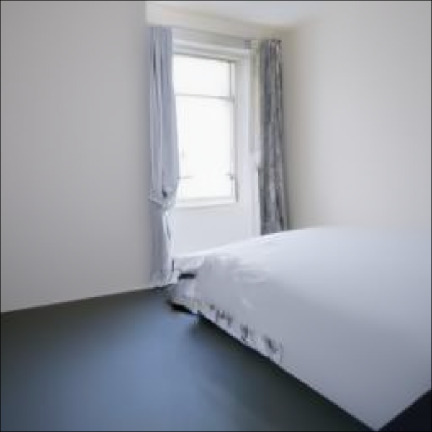
Figure 5: Outpainting and inpainting experiments. The remaining samples are displayed in Section C.2.2

6 Conclusion

In this paper, we introduced DCPS to address Bayesian linear inverse problems with DDM priors while avoiding any problem-specific extra training. Our divide-and-conquer strategy allows to reduce the approximation error incurred by existing approaches, while our variational framing constitutes a principled method for estimating the backward kernels. DCPS is more robust to parameter tuning in comparison with its competitors. Our method invites extensions and improvements in several respects. For instance, we aim to investigate the role of $\sigma_{y,\ell}$, how it impacts the mixing of the unadjusted Langevin algorithm and provide guidelines as regards to its tuning. Designing principled potentials for non-linear inverse problems is also one important direction of research.

Acknowledgments.

The work of Y.J. has been supported by Technology Innovation Institute (TII), project Fed2Learn. The work of Eric Moulines has been partly funded by the European Union (ERC-2022-SYG-OCEAN-101071601). Views and opinions expressed are however those of the author(s) only and do not necessarily reflect those of the European Union or the European Research Council Executive Agency. Neither the European Union nor the granting authority can be held responsible for them.

Appendix A Methodology details

A.1 Variational approximations

In this section we provide the detailed losses for the variational approximations.

Explicit Gaussian parameterization.

In order to optimize the objective (4.13) we use stochastic gradient descent (SGD). We consider two gradient estimates. The first gradient estimate is unbiased as we use the exact expression of $\tilde{g}^{y,\ell}_{m}$ and only estimate the expectation over $Z$:

$$\nabla_{\hat{\mu}_{m},\hat{s}_{m}}\mathcal{L}_{m}(x_{m+1};\hat{\mu}_{m},\hat{s}_{m}) \approx\nabla_{\hat{\mu}_{m},\hat{s}_{m}}\widehat{\mathcal{L}}_{m}(x_{m+1},Z_{m};\hat{\mu}_{m},\hat{s}_{m})$$

$$\vcentcolon=\nabla_{\hat{\mu}_{m},\hat{s}_{m}}\left\{-\log\tilde{g}^{y,\ell}_{m}(\hat{\mu}_{m}+(I_{d_{x}}\mathrm{e}^{\hat{s}_{m}})Z_{m})+\frac{\|\hat{\mu}_{m}-\mu_{m|m+1}(x_{m+1})\|^{2}}{2\sigma^{2}_{m|m+1}}\vphantom{\sum_{i=1}^{d_{x}}\left(\hat{s}_{m,i}-\frac{\mathrm{e}^{\hat{s}_{m,i}}}{\sigma^{2}_{m|m+1}}\right)}\right.$$

$$\left.\hskip 28.45274pt-\frac{1}{2}\sum_{i=1}^{d_{x}}\left(\hat{s}_{m,i}-\frac{\mathrm{e}^{\hat{s}_{m,i}}}{\sigma^{2}_{m|m+1}}\right)\right\},$$

where $Z_{m}\sim\mathcal{N}(0_{d_{x}},I_{d_{x}})$. As for the second gradient estimate, we use the biased estimate

$$\log\tilde{g}^{y,\ell}_{m}(x_{m})\approx\log g^{y}_{{k_{\ell}}}(\mu_{{k_{\ell}}|m}(x_{m})+\sigma_{{k_{\ell}}|m}\tilde{Z}_{{k_{\ell}}|m}),$$

where $\tilde{Z}_{{k_{\ell}}|m}\sim\mathcal{N}(0_{d_{x}},I_{d_{x}})$. This allows us to avoid computing the eigendecomposition of the forward operator $A$. The resulting biased gradient estimate is

$$\nabla_{\hat{\mu}_{m},\hat{s}_{m}}\widetilde{\mathcal{L}}_{m}(x_{m+1},Z_{m},\tilde{Z}_{{k_{\ell}}|m};\hat{\mu}_{m},\hat{s}_{m}) \vcentcolon=\nabla_{\hat{\mu}_{m},\hat{s}_{m}}\left\{-\log g^{y}_{{k_{\ell}}}(\mu_{{k_{\ell}}|m}(\hat{\mu}_{m}+(I_{d_{x}}\mathrm{e}^{\hat{s}_{m}})Z_{m})+\sigma_{{k_{\ell}}|m}\tilde{Z}_{{k_{\ell}}|m})\vphantom{\left(\hat{s}_{m,i}-\frac{\mathrm{e}^{\hat{s}_{m,i}}}{\sigma^{2}_{m|m+1}}\right)}\right.$$

$$\left.+\frac{\|\hat{\mu}_{m}-\mu_{m|m+1}(x_{m+1})\|^{2}}{2\sigma^{2}_{m|m+1}}-\frac{1}{2}\sum_{i=1}^{d_{x}}\left(\hat{s}_{m,i}-\frac{\mathrm{e}^{\hat{s}_{m,i}}}{\sigma^{2}_{m|m+1}}\right)\right\}\,.$$

In practice we found that this estimate works well already on all the examples we considered, with no significant performance decline.

For the optimization of the objective we found that normalized SGD outperforms Adam and we use it in all our experiments. The complete version of Algorithm 1 that we implement in our experiments is given in Algorithm 2.

Algorithm 2 Divide-and-Conquer Posterior Sampler (DCPS)

  Input: $y$, timesteps $({k_{\ell}})_{\ell=0}^{L}$, numbers $G$ and $L$ of gradient and Langevin steps, respectively, TULA step-size $\gamma$.Initial sample $X^{y}_{k_{L+1}}\sim\mathcal{N}(0_{d_{x}},I_{d_{x}})$;

  for $\ell=L$ to $0$ do

     //Tamed Langevin steps to target (4.11); see (4.15).

     $X^{y,\ell}_{{k_{\ell+1}},1}=X^{y}_{{k_{\ell+1}}};$

     for $h=1$ to $K$ do

        $X^{y,\ell}_{{k_{\ell+1}},h+1}=X^{y,\ell}_{{k_{\ell+1}},h}+\gamma G^{y,\ell}_{\gamma}(X^{y,\ell}_{{k_{\ell+1}},h})+\sqrt{2\gamma}Z_{h}\,,$ where $Z_{h}\sim\mathcal{N}(0_{d_{x}},I_{d_{x}})$;

     end for

     $X^{y,\ell}_{{k_{\ell+1}}}=X^{y,\ell}_{{k_{\ell+1}},K+1}$;

     for $m={k_{\ell+1}}-1$ to ${k_{\ell}}$ do

        $\hat{\mu}_{m,1}=\mu_{m|m+1}(X^{y,\ell}_{m+1}),\,\hat{s}_{m,1}=\log\sigma^{2}_{{k_{\ell}}|m+1}\cdot\mathbf{1}_{d_{x}}$;

        //Optimization of the variational loss; see (4.13).

        for $g=1$ to $G$ do

           $(Z_{m,g},Z_{{k_{\ell}}|m,g})\overset{\operatorname{iid}}{\sim}\mathcal{N}(0_{d_{x}},I_{d_{x}})$;

           $\hat{\mu}_{m,g+1}=\hat{\mu}_{m,g}-\|\nabla_{\hat{\mu}_{m}}\widetilde{\mathcal{L}}_{m}(X^{y,\ell}_{m+1},Z_{m,g},\tilde{Z}_{{k_{\ell}}|m,g};\hat{\mu}_{m},\hat{s}_{m})\|^{-1}\nabla_{\hat{\mu}_{m}}\widetilde{\mathcal{L}}_{m}(X^{y,\ell}_{m+1},Z_{m,g},\tilde{Z}_{{k_{\ell}}|m,g};\hat{\mu}_{m},\hat{s}_{m})$;

           $\hat{s}_{m,g+1}=\hat{s}_{m,g}-\|\nabla_{\hat{s}_{m}}\widetilde{\mathcal{L}}_{m}(X^{y,\ell}_{m+1},Z_{m,g},\tilde{Z}_{{k_{\ell}}|m,g};\hat{\mu}_{m},\hat{s}_{m})\|^{-1}\nabla_{\hat{s}_{m}}\widetilde{\mathcal{L}}_{m}(X^{y,\ell}_{m+1},Z_{m,g},\tilde{Z}_{{k_{\ell}}|m,g};\hat{\mu}_{m,g},\hat{s}_{m,g})$;

        end for

        $X^{y,\ell}_{m}=\hat{\mu}_{m,G+1}+(I_{d_{x}}\mathrm{e}^{\hat{s}_{m,G+1}/2})\varepsilon$, where $\varepsilon\sim\mathcal{N}(0_{d_{x}},I_{d_{x}})$;

     end for

     $X^{y}_{{k_{\ell}}}=X^{y,\ell}_{{k_{\ell}}}$;

  end for

Implicit Gaussian parameterization.

We can avoid the expensive matrix inversion involved in the exact computation of $\tilde{g}^{y,\ell}_{m}$ by considering a implicit Gaussian parameterization of $r^{y,\ell}_{m|m+1}(\cdot|x_{m})$. Consider instead the following parameterization of the backward kernel:

$$r^{y,\ell}_{m|m+1}(\mathrm{d}x_{m}|x_{m+1})\vcentcolon=\int\smash{q}^{\eta}_{m|{k_{\ell}},m+1}(\mathrm{d}x_{m}|x_{k_{\ell}},x_{m+1})\,r^{y,\ell}_{{k_{\ell}}|m+1}(\mathrm{d}x_{k_{\ell}}|x_{m+1})\,,$$ (A.1)

where $r^{y,\ell}_{{k_{\ell}}|m+1}(\cdot|x_{m+1})\in\mathcal{G}_{\mathrm{D}}$ and $\smash{q}^{\eta}_{m|{k_{\ell}},m+1}(\cdot|x_{k_{\ell}},x_{m+1})$ is a Gaussian distribution with mean

$$\mu_{m|{k_{\ell}},m+1}(x_{k_{\ell}},x_{m+1})\vcentcolon=\sqrt{\alpha_{m}/\alpha_{{k_{\ell}}}}x_{k_{\ell}}+\sqrt{1-\alpha_{m}/\alpha_{{k_{\ell}}}-\sigma^{2}_{k}}\frac{x_{m+1}-\sqrt{\alpha_{m+1}/\alpha_{{k_{\ell}}}}x_{k_{\ell}}}{\sqrt{1-\alpha_{m+1}/\alpha_{{k_{\ell}}}}}$$

and covariance matrix $\sigma^{2}_{m|{k_{\ell}},m+1}I_{d_{x}}$, with

$$\sigma^{2}_{m|{k_{\ell}},m+1}\vcentcolon=\eta^{2}\left(1-\frac{\alpha_{m}}{\alpha_{{k_{\ell}}}}\right)\left(1-\frac{\alpha_{m+1}}{{k_{\ell}}}\right)\left/\left(1-\frac{\alpha_{m+1}}{\alpha_{m}}\right)\right.\,.$$ (A.2)

As a result of this parameterization, (A.1) is also Gaussian. We now write $r^{y,\ell}_{{k_{\ell}},m|m+1}(\cdot|x_{t+1})$ as a shorthand for the joint distribution on the r.h.s. in (A.1). Then, by the data processing inequality (Van Erven & Harremos, 2014) and the definition of the approximate potential (4.10),

$$\mathsf{KL}(r^{y,\ell}_{m|m+1}(\cdot|x_{m+1})\parallel\smash{\tilde{p}}^{y,\ell}_{m|m+1}(\cdot|x_{m+1}))\leq\mathsf{KL}(r^{y,\ell}_{{k_{\ell}},m|m+1}(\cdot|x_{m+1})\parallel\smash{\tilde{p}}^{y,\ell}_{{k_{\ell}},m|m+1}(\cdot|x_{m+1}))\,,$$

where

$$\smash{\tilde{p}}^{y,\ell}_{{k_{\ell}},m|m+1}(\mathrm{d}(x_{k_{\ell}},x_{m})|x_{m+1})\propto g^{y,\ell}_{{k_{\ell}}}(x_{k_{\ell}})\,\smash{\tilde{p}}_{{k_{\ell}},m|m+1}(\mathrm{d}(x_{k_{\ell}},x_{m})|x_{m+1})$$ (A.3)

and

$$\smash{\tilde{p}}_{{k_{\ell}},m|m+1}(\mathrm{d}(x_{k_{\ell}},x_{m})|x_{m+1})\vcentcolon=\smash{\tilde{p}}_{{k_{\ell}}|m}(\mathrm{d}x_{k_{\ell}}|x_{m})\,\smash{p}_{m|m+1}(\mathrm{d}x_{m}|x_{m+1})\,.$$

Next, the KL divergence on the r.h.s. can be written as

$$\mathsf{KL}(r^{y,\ell}_{{k_{\ell}},m|m+1}(\cdot|x_{m+1})\parallel\smash{\tilde{p}}^{y,\ell}_{{k_{\ell}},m|m+1}(\cdot|x_{m+1}))\\ =-\int\log\smash{g^{y}_{{k_{\ell}}}}(x_{k_{\ell}})\,r^{y,\ell}_{{k_{\ell}}|m+1}(\mathrm{d}x_{k_{\ell}}|x_{m+1})+\mathsf{KL}(r^{y,\ell}_{{k_{\ell}},m|m+1}(\cdot|x_{m+1})\parallel\smash{\tilde{p}}_{{k_{\ell}},m|m+1}(\cdot|x_{m+1}))+\mbox{const.}$$

Then, letting $r^{y,\ell}_{{k_{\ell}}|m+1}(\mathrm{d}x_{k_{\ell}}|x_{m+1})=\phi(\mathrm{d}x_{k_{\ell}};\hat{\mu}_{{k_{\ell}}|m},I_{d_{x}}\mathrm{e}^{\hat{s}_{{k_{\ell}}|m}})$, we obtain

$$\mathsf{KL}(r^{y,\ell}_{{k_{\ell}},m|m+1}(\cdot|x_{t+1})\parallel\smash{\tilde{p}}^{y,\ell}_{{k_{\ell}},m|m+1}(\cdot|x_{t+1}))$$

$$\hskip 28.45274pt=\frac{1}{\sigma^{2}_{y,\ell}}\|\sqrt{\alpha_{{k_{\ell}}}}y-A\hat{\mu}_{{k_{\ell}}|m+1}\|^{2}+\frac{1}{\sigma^{2}_{y,\ell}}\operatorname{tr}(A(I_{d_{x}}\mathrm{e}^{\hat{s}_{{k_{\ell}}|m+1}})A^{\intercal})$$

$$\hskip 42.67912pt+\int\mathsf{KL}(\smash{q}^{\eta}_{m|{k_{\ell}},m+1}(\cdot|x_{k_{\ell}},x_{m+1})\parallel\smash{p}_{m|m+1}(\cdot|x_{m+1}))\,r^{y,\ell}_{{k_{\ell}}|m+1}(\mathrm{d}x_{k_{\ell}}|x_{m+1})$$

$$\hskip 42.67912pt+\int\int\log\frac{r^{y,\ell}_{{k_{\ell}}|m+1}(x_{k_{\ell}}|x_{m+1})}{\smash{\tilde{p}}_{{k_{\ell}}|m}(x_{k_{\ell}}|x_{m})}\,\smash{q}^{\eta}_{m|{k_{\ell}},m+1}(\mathrm{d}x_{m}|x_{k_{\ell}},x_{m+1})r^{y,\ell}_{{k_{\ell}}|m+1}(\mathrm{d}x_{k_{\ell}}|x_{m+1})\,.$$

The first, integrated KL can be computed in a closed form, whereas for the second term we can compute the inner KL and then estimate the integral and for the third term we can also compute exactly the first integral and then use a MC estimate. Note that this loss involves the computation of the trace $\operatorname{tr}(A(I_{d_{x}}\mathrm{e}^{\hat{s}_{{k_{\ell}}|m+1}})A^{\intercal})$ which in turn requires the multiplication of a ${d_{y}}\times{d_{x}}$ matrix by a ${d_{x}}\times{d_{y}}$ ditto. It is possible to further reduce the computational cost by resorting to an unbiased estimate of this trace using the Hutchinson trace estimator (Hutchinson, 1989).

A.2 Approximate Gibbs sampler

We now detail how one can use an approximate Gibbs sampler to sample from $p^{y,\ell}_{{k_{\ell+1}}}$. We assume that $\eta=1$ for convenience. By (4.6) and (4.8), $p^{y,\ell}_{{k_{\ell+1}}}$ is the marginal of the joint distribution

$$p^{y,\ell}_{{k_{\ell}},{k_{\ell+1}}}(\mathrm{d}(x_{k_{\ell}},x_{k_{\ell+1}}))\propto\smash{g^{y}_{{k_{\ell}}}}(x_{k_{\ell}})\,p_{{k_{\ell}},{k_{\ell+1}}}(\mathrm{d}(x_{k_{\ell}},x_{k_{\ell+1}}))\,.$$

Therefore, we can use Gibbs sampling to sample from it. Indeed, under this joint distribution, the law of $X_{k_{\ell}}|X_{k_{\ell+1}}=x_{k_{\ell+1}}$ is given by

$$\smash{p}^{y,\ell}_{{k_{\ell}}|{k_{\ell+1}}}(\mathrm{d}x_{k_{\ell}}|x_{k_{\ell+1}})\propto g^{y}_{{k_{\ell}}}(x_{k_{\ell}})\smash{p}_{{k_{\ell}}|{k_{\ell+1}}}(\mathrm{d}x_{k_{\ell}}|x_{k_{\ell+1}})\,,$$

and we may, as previously, approximate it using the Gaussian approximation (4.9) of $\smash{p}_{{k_{\ell}}|{k_{\ell+1}}}(\mathrm{d}x_{k_{\ell}}|x_{k_{\ell+1}})$. The resulting approximation, which we denote by $\smash{\tilde{p}}^{y,\ell}_{{k_{\ell}}|{k_{\ell+1}}}(\cdot|x_{k_{\ell+1}})$, can then be computed in a closed form since $\smash{g^{y}_{{k_{\ell}}}}$ is a Gaussian distribution whose mean is linear in $x_{k_{\ell}}$.

We turn to the second conditional $X_{k_{\ell+1}}|X_{k_{\ell}}=x_{k_{\ell}}$, which is given by

$$\smash{p}_{{k_{\ell+1}}|{k_{\ell}}}(\mathrm{d}x_{k_{\ell+1}}|x_{k_{\ell}})\propto p_{{k_{\ell+1}}}(\mathrm{d}x_{k_{\ell+1}})\smash{p}_{{k_{\ell}}|{k_{\ell}}+1}(x_{k_{\ell}}|x_{k_{\ell+1}}).$$

Assuming that $\smash{p}_{{k_{\ell}}|{k_{\ell+1}}}(\mathrm{d}x_{{k_{\ell}}}|x_{{k_{\ell+1}}})$ and $p_{{k_{\ell}}}$ are approximately equal to $q_{{k_{\ell}}|{k_{\ell+1}}}(\mathrm{d}x_{{k_{\ell}}}|x_{k_{\ell+1}})$ and $q_{{k_{\ell}}}$, respectively, it holds that $\smash{p}_{{k_{\ell+1}}|{k_{\ell}}}(\mathrm{d}x_{{k_{\ell+1}}}|x_{k_{\ell}})$ is approximately equal to $q_{{k_{\ell+1}}|{k_{\ell}}}(\mathrm{d}x_{{k_{\ell+1}}}|x_{k_{\ell}})$, which allows us to draw an approximate sample by simply using the forward transition (2.2). We further detail both steps below.

Conditional $X_{k_{\ell+1}}|X_{k_{\ell}}$.

First, we assume that $\eta=1$, since in this case we have that (see Song et al., 2021a, Section 4.1)

$$\smash{q}^{\eta}_{m|0,m+1}(\mathrm{d}x_{m}|x_{0},x_{m+1})=\frac{q_{m|0}(\mathrm{d}x_{m}|x_{0})q_{m+1|m}(x_{m+1}|x_{m})}{q_{m+1|0}(x_{m+1}|x_{0})}\,,$$

where $q_{m+1|m}(\mathrm{d}x_{m+1}|x_{m})$ is the Markov transition associated to (2.2). Using (2.7) and the definition of the backward kernel $\smash{q}_{0|m+1}$ yields

$$\smash{q}^{\eta}_{m|m+1}(\mathrm{d}x_{m}|x_{m+1})=\frac{q_{m}(\mathrm{d}x_{m})q_{m+1|m}(x_{m+1}|x_{m})}{q_{m+1}(x_{m+1})}\,.$$ (A.4)

Hence, assuming that $p_{{k_{\ell}}}$ is approximately equal to $q_{{k_{\ell}}}$, we find that

$$p_{{k_{\ell}}}(\mathrm{d}x_{k_{\ell}})q_{{k_{\ell+1}}|{k_{\ell}}}(\mathrm{d}x_{m+1}|x_{k_{\ell}})\approx p_{{k_{\ell+1}}}(\mathrm{d}x_{k_{\ell+1}})\smash{p}_{{k_{\ell}}|{k_{\ell+1}}}(\mathrm{d}x_{k_{\ell}}|x_{k_{\ell+1}})\,,$$

and we may thus use the forward transition kernel $\smash{q}_{{k_{\ell+1}}|{k_{\ell}}}(\mathrm{d}x_{k_{\ell+1}}|{k_{\ell}})$ as the reversal of $\smash{p}_{{k_{\ell}}|{k_{\ell+1}}}(\mathrm{d}x_{k_{\ell}}|x_{k_{\ell+1}})$.

Conditional $X_{k_{\ell}}|X_{k_{\ell+1}}$.

We remind the reader that by (4.6) and (4.8), $p^{y,\ell}_{{k_{\ell+1}}}$ is the marginal of the joint distribution

$$p^{y}_{{k_{\ell}},{k_{\ell+1}}}(\mathrm{d}(x_{k_{\ell}},x_{k_{\ell+1}}))\propto\smash{g^{y}_{{k_{\ell}}}}(x_{k_{\ell}})\,p_{{k_{\ell}},{k_{\ell+1}}}(\mathrm{d}(x_{k_{\ell}},x_{k_{\ell+1}}))\,,$$

and under this joint distribution, the law of $X_{k_{\ell}}|X_{k_{\ell+1}}=x_{k_{\ell+1}}$ is

$$\smash{p}^{y,\ell}_{{k_{\ell}}|{k_{\ell+1}}}(\mathrm{d}x_{k_{\ell}}|x_{k_{\ell+1}})\propto g^{y}_{{k_{\ell}}}(x_{k_{\ell}})\,\smash{p}_{{k_{\ell}}|{k_{\ell+1}}}(\mathrm{d}x_{k_{\ell}}|x_{k_{\ell+1}})\,.$$

We approximate this distribution by $\smash{\tilde{p}}^{y,\ell}_{{k_{\ell}}|{k_{\ell+1}}}(\mathrm{d}x_{{k_{\ell}}}|x_{k_{\ell+1}})$ using the Gaussian approximation (4.9) of $\smash{p}_{{k_{\ell}}|{k_{\ell+1}}}(\mathrm{d}x_{k_{\ell}}|x_{k_{\ell+1}})$, i.e.,

$$\smash{\tilde{p}}^{y,\ell}_{{k_{\ell}}|{k_{\ell+1}}}(\mathrm{d}x_{k_{\ell}}|x_{k_{\ell+1}})\propto g^{y}_{{k_{\ell}}}(x_{k_{\ell}})\,\smash{\tilde{p}}_{{k_{\ell}}|{k_{\ell+1}}}(\mathrm{d}x_{k_{\ell}}|x_{k_{\ell+1}})\,.$$ (A.5)

Using (Bishop, 2006, Eq. 2.116) and definitions (3.5) (4.9), we obtain that

$$\smash{\tilde{p}}^{y,\ell}_{{k_{\ell}}|{k_{\ell+1}}}(x_{k_{\ell}}|x_{k_{\ell+1}})=\phi\left(x_{k_{\ell}};\Sigma^{y,\ell}_{{k_{\ell+1}}}\left(\frac{A^{\intercal}y}{\sigma^{2}_{y,\ell}}+\frac{\mu_{{k_{\ell}}|{k_{\ell+1}}}(x_{k_{\ell+1}})}{\sigma^{2}_{{k_{\ell}}|{k_{\ell+1}}}}\right),\Sigma^{y,\ell}_{{k_{\ell+1}}}\right)\,,$$ (A.6)

where

$$\Sigma^{y,\ell}_{{k_{\ell+1}}}\vcentcolon=\left(\frac{1}{\sigma^{2}_{{k_{\ell}}|{k_{\ell+1}}}}I_{d_{x}}+\frac{1}{\sigma^{2}_{y,\ell}}A^{\intercal}A\right)^{-1}\,.$$ (A.7)

Algorithm 3 One step of approximate Gibbs sampler with matrix inversion

1:  Input: Observation $y$, number $M$ of Gibbs steps, initial sample $X^{y,\ell}_{{k_{\ell+1}}}$

2:  Output: $X^{y,\ell}_{{k_{\ell+1}},M+1}$

3:  Initial sample $X^{y,\ell}_{{k_{\ell+1}},1}=X^{y,\ell}_{{k_{\ell+1}}}$;

4:  for $i=1$ to $M$ do

5:     $X^{y,\ell}_{{k_{\ell}},i}\sim\smash{\tilde{p}}^{y,\ell}_{{k_{\ell}}|{k_{\ell+1}}}(\cdot|X^{y,\ell}_{{k_{\ell+1}},i})$ following (A.6);

6:     $X^{y,\ell}_{{k_{\ell+1}},i+1}=\sqrt{\alpha_{{k_{\ell+1}}}/\alpha_{{k_{\ell}}}}X^{y,\ell}_{{k_{\ell}},i}+\sqrt{1-\alpha_{{k_{\ell+1}}}/\alpha_{{k_{\ell}}}}Z_{i}$, where $Z_{i}\sim\mathcal{N}(0_{d_{x}},I_{d_{x}})$;

7:  end for

RePaint.

The approximate Gibbs sampler perspective allows us to re-frame the RePaint algorithm of Lugmayr et al. (2022) as a special case of our framework. For the sake of simplicity, we assume that $A$ is rectangular unit diagonal, i.e., that we only observe the first ${d_{y}}$ coordinates of a sample from the prior. We denote by $\overline{X}$ the first ${d_{y}}$ coordinates of $X\in\mathbb{R}^{d_{x}}$ and by $\underline{X}$ the remaining ones. Then, step 5 of Algorithm 3 is equivalent to setting $X^{y}_{{k_{\ell}},i}=[\overline{X}^{y,\ell}_{{k_{\ell+1}},i},\underline{X}^{y,\ell}_{{k_{\ell+1}},i}]$, where

$$\overline{X}^{y,\ell}_{{k_{\ell}},i} =\frac{\sigma^{2}_{{k_{\ell}}|{k_{\ell+1}}}}{\sigma^{2}_{y,\ell}+\sigma^{2}_{{k_{\ell}}|{k_{\ell+1}}}}y_{{k_{\ell}}}+\frac{\sigma^{2}_{y,\ell}}{\sigma^{2}_{y,\ell}+\sigma^{2}_{{k_{\ell}}|{k_{\ell+1}}}}\overline{\mu_{{k_{\ell}}|{k_{\ell+1}}}(X^{y}_{{k_{\ell+1}},i})}+\frac{\sigma^{2}_{y,\ell}\sigma^{2}_{{k_{\ell}}|{k_{\ell+1}}}}{\sigma^{2}_{y,\ell}+\sigma^{2}_{{k_{\ell}}|{k_{\ell+1}}}}\overline{Z}_{i}\,,$$

$$\underline{X}^{y,\ell}_{{k_{\ell}},i} =\underline{\mu_{{k_{\ell}}|{k_{\ell+1}}}(X^{y}_{{k_{\ell+1}},i})}+\sigma^{2}_{{k_{\ell}}|{k_{\ell+1}}}\underline{Z}_{i}.$$

Thus, if we choose $L=n$, implying that ${k_{\ell}}=\ell$, we recover a generalization of the RePaint algorithm. In the specific case of an inverse problem with $\sigma_{y}=0$, we can, setting for all $\ell$ $\sigma_{y,\ell}=0$ and $y_{\ell}=\sqrt{\alpha_{\ell}}\,y+\sqrt{1-\alpha_{\ell}}Z_{\ell}$ and $Z_{\ell}$ are i.i.d. standard Gaussian samples, recover the Algorithm 1 in Lugmayr et al. (2022).

Variational approximation.

When this matrix inversion is prohibitively expensive, which is typically the case in very large dimensions, we propose the use of a diagonal Gaussian variational approximation of (A.5). This is done by solving

$$\operatorname*{argmin}_{r^{y,\ell}_{{k_{\ell}}|{k_{\ell+1}}}(\cdot|x_{\ell+1})\in\mathcal{G}_{\mathrm{D}}}\mathsf{KL}(r^{y,\ell}_{{k_{\ell}}|{k_{\ell+1}}}(\cdot|x_{\ell+1})\parallel\smash{\tilde{p}}^{y,\ell}_{{k_{\ell}}|{k_{\ell+1}}}(\cdot|x_{\ell+1}))\,,$$

where the KL can be computed in a closed form. Indeed, this is equivalent to the following minimization problem

$$\operatorname*{argmin}_{(\hat{\mu}_{{k_{\ell|{k_{\ell+1}}}}},s_{{k_{\ell}}|{k_{\ell+1}}})\in\mathbb{R}^{d_{x}}\times\mathbb{R}^{d_{x}}}\mathcal{L}^{y,\ell}_{{k_{\ell}}|{k_{\ell+1}}}(\hat{\mu}_{{k_{\ell}}|{k_{\ell+1}}},s_{{k_{\ell}}|{k_{\ell+1}}};x_{{k_{\ell+1}}}),$$

where

$$\mathcal{L}^{y,\ell}_{{k_{\ell}}|{k_{\ell+1}}}(\hat{\mu}_{{k_{\ell}}|{k_{\ell+1}}},s_{{k_{\ell}}|{k_{\ell+1}}};x_{{k_{\ell+1}}})\vcentcolon=\frac{1}{\sigma^{2}_{y,\ell}}\|\sqrt{\alpha_{{k_{\ell}}}}y-A\hat{\mu}_{{k_{\ell}}|{k_{\ell+1}}}\|^{2}+\frac{1}{\sigma^{2}_{y,\ell}}\operatorname{tr}(A(I_{d_{x}}\mathrm{e}^{s_{{k_{\ell}}|{k_{\ell+1}}}})A^{\intercal})\\ +\frac{1}{2\sigma^{2}_{{k_{\ell}}|{k_{\ell+1}}}}\|\hat{\mu}_{{k_{\ell}}|{k_{\ell+1}}}-\mu_{{k_{\ell}}|{k_{\ell+1}}}(x_{{k_{\ell+1}}})\|^{2}-\frac{1}{2}\sum_{i=1}^{d_{x}}\left(s_{{k_{\ell}}|{k_{\ell+1}},i}-\frac{\mathrm{e}^{s_{{k_{\ell}}|{k_{\ell+1}},i}}}{\sigma^{2}_{{k_{\ell}}|{k_{\ell+1}}}}\right)\,.$$

We optimize this loss using SGD, and the complete algorithm is summarized in Algorithm 4.

Algorithm 4 One step of the approximate Gibbs sampler with diagonal Gaussian approximation

1:  Input: Observation $y$, number $M$ of Gibbs steps, initial sample $X^{y,\ell}_{{k_{\ell+1}}}$, number $V$ of VI steps

2:  Output: $X^{y,\ell}_{{k_{\ell+1}},M+1}$

3:  Initial sample $X^{y,\ell}_{{k_{\ell+1}},1}=X^{y,\ell}_{{k_{\ell+1}}}$;

4:  for $i=1$ to $M$ do

5:     Set $\hat{\mu}_{1}=\mu_{{k_{\ell}}|{k_{\ell+1}}}$, $s_{1}=\log\sigma^{2}_{{k_{\ell}}|{k_{\ell+1}}}\mathbf{1}_{d_{x}}$;

6:     for $j=1$ to $V$ do

7:        // $\hat{x}^{\theta}_{0|{k_{\ell+1}}}(X^{y,\ell}_{{k_{\ell+1}},i})$ is computed only once.

8:        $\hat{\mu}_{j+1}=\hat{\mu}_{j}-\|\nabla_{\mu}\mathcal{L}^{y,\ell}_{{k_{\ell}}|{k_{\ell}}+1}(\hat{\mu}_{j},s_{j};X^{y,\ell}_{{k_{\ell+1}},i})\|^{-1}\nabla_{\mu}\mathcal{L}^{y,\ell}_{{k_{\ell}}|{k_{\ell}}+1}(\hat{\mu}_{j},s_{j};X^{y,\ell}_{{k_{\ell+1}},i})$;

9:        $s_{j+1}=s_{j}-\|\nabla_{s}\mathcal{L}^{y,\ell}_{{k_{\ell}}|{k_{\ell}}+1}(\hat{\mu}_{j},s_{j};X^{y,\ell}_{{k_{\ell+1}},i})\|^{-1}\nabla_{s}\mathcal{L}^{y,\ell}_{{k_{\ell}}|{k_{\ell}}+1}(\hat{\mu}_{j},s_{j};X^{y,\ell}_{{k_{\ell+1}},i})$;

10:     end for

11:     $X^{y,\ell}_{{k_{\ell}},i}\sim\mathcal{N}(\hat{\mu}_{V+1},I_{d_{x}}\mathrm{e}^{s_{V+1}/2})$;

12:     $X^{y,\ell}_{{k_{\ell+1}},i+1}=\sqrt{\alpha_{{k_{\ell+1}}}/\alpha_{{k_{\ell}}}}X^{y,\ell}_{{k_{\ell}},i}+\sqrt{1-\alpha_{{k_{\ell+1}}}/\alpha_{{k_{\ell}}}}Z_{i}$, where $Z_{i}\sim\mathcal{N}(0_{d_{x}},I_{d_{x}})$;

13:  end for

Appendix B Proofs

Proof of Lemma 4.1.

We remind the reader that

$$\begin{cases}Y&=AX_{0}+\sigma_{y}Z_{0}\,,\\ X_{k_{\ell}}&=\sqrt{\alpha_{{k_{\ell}}}}X_{0}+\sqrt{1-\alpha_{{k_{\ell}}}}\varepsilon_{\ell}\,,\\ Y_{k_{\ell}}&=AX_{k_{\ell}}+\sigma_{y,\ell}Z_{\ell}\,,\end{cases}$$ (B.1)

where $(Z_{0},Z_{\ell})\sim\mathcal{N}(0_{d_{y}},I_{d_{y}})^{\otimes 2}$, $\varepsilon\sim\mathcal{N}(0_{d_{x}},I_{d_{y}})$ and is independent of $(Z_{0},Z_{\ell})$. Let $(\tilde{Z}_{0},\tilde{Z}_{\ell})\sim\mathcal{N}(0_{d_{y}},I_{d_{y}})^{\otimes 2}$ and independent of $\varepsilon$. Then it holds that

$$\sigma_{y,\ell}Z_{\ell}\;\smash{\overset{\mathcal{L}}{=}}\;\sqrt{\alpha_{{k_{\ell}}}}\sigma_{y}\tilde{Z}_{0}+\sqrt{\sigma^{2}_{y,\ell}-\alpha_{{k_{\ell}}}\sigma_{y}^{2}}\tilde{Z}_{\ell}\,,$$

and hence,

$$Y_{k_{\ell}} \;\smash{\overset{\mathcal{L}}{=}}\;\sqrt{\alpha_{{k_{\ell}}}}AX_{0}+\sqrt{1-\alpha_{{k_{\ell}}}}A\varepsilon_{\ell}+\sigma_{y,\ell}Z_{\ell}$$

$$\;\smash{\overset{\mathcal{L}}{=}}\;\sqrt{\alpha_{{k_{\ell}}}}AX_{0}+\sqrt{1-\alpha_{{k_{\ell}}}}A\varepsilon_{\ell}+\sqrt{\alpha_{{k_{\ell}}}}\sigma_{y}\tilde{Z}_{0}+\sqrt{\sigma^{2}_{y,\ell}-\alpha_{{k_{\ell}}}\sigma_{y}^{2}}\tilde{Z}_{\ell}\,.$$

Using then the definition of $Y$, we obtain

$$Y_{k_{\ell}}\;\smash{\overset{\mathcal{L}}{=}}\;\sqrt{\alpha_{{k_{\ell}}}}\,Y+\sqrt{1-\alpha_{{k_{\ell}}}}A\varepsilon_{\ell}+\sqrt{\sigma^{2}_{y,\ell}-\alpha_{{k_{\ell}}}\sigma_{y}^{2}}\tilde{Z}_{\ell}\,,$$

and, letting $C$ denote the square root of the symmetric positive definite matrix $(1-\alpha_{{k_{\ell}}})AA^{\intercal}+(\sigma^{2}_{y,\ell}-\alpha_{{k_{\ell}}}\sigma_{y}^{2})I_{d_{y}}$ we have that

$$\sqrt{1-\alpha_{{k_{\ell}}}}A\varepsilon_{\ell}+\sqrt{\sigma^{2}_{y,\ell}-\alpha_{{k_{\ell}}}\sigma_{y}^{2}}\tilde{Z}_{\ell}\;\smash{\overset{\mathcal{L}}{=}}\;C\overline{Z}_{\ell}\,.$$

It then follows that

$$Y_{k_{\ell}}\;\smash{\overset{\mathcal{L}}{=}}\;\sqrt{\alpha_{{k_{\ell}}}}\,Y+C\overline{Z}_{\ell}\,.$$

∎

B.1 Proof of Proposition 4.2

We remind the reader that in the specific case of $\eta=1$, the bridge kernel of DDIM is given by

$$\smash{q}^{\eta}_{{k_{\ell}}|0,m}(\mathrm{d}x_{k_{\ell}}|x_{0},x_{m})=\phi\left(\mathrm{d}x_{k_{\ell}};\frac{\sqrt{\alpha_{{k_{\ell}}}{}}(1-\alpha_{m}/\alpha_{{k_{\ell}}})}{1-\alpha_{m}}x_{0}+\frac{\sqrt{\alpha_{m}/\alpha_{{k_{\ell}}}}(1-\alpha_{{k_{\ell}}})}{1-\alpha_{m}}x_{m},\frac{(1-\alpha_{{k_{\ell}}})(1-\alpha_{m}/\alpha_{{k_{\ell}}})}{1-\alpha_{m}}I_{d_{x}}\right)$$

and can be alternatively expressed in terms of transitions of the forward process

$$\smash{q}^{\eta}_{{k_{\ell}}|0,m}(\mathrm{d}x_{k_{\ell}}|x_{0},x_{m})=\frac{\smash{q}_{m|{k_{\ell}}}(x_{m}|x_{k_{\ell}})\smash{q}_{{k_{\ell}}|0}(\mathrm{d}x_{k_{\ell}}|x_{0})}{\smash{q}_{m|0}(x_{m}|x_{0})}\,.$$ (B.2)

Proof of Proposition 4.2.

Under the assumptions of the proposition, we have, for all $m>{k_{\ell}}$,

$$\smash{p}_{{k_{\ell}}|m}(\mathrm{d}x_{k_{\ell}}|x_{m})=\smash{q}^{\eta}_{{k_{\ell}}|m}(\mathrm{d}x_{k_{\ell}}|x_{m})=\int\smash{q}^{\eta}_{{k_{\ell}}|0,m}(\mathrm{d}x_{k_{\ell}}|x_{0},x_{m})\,\smash{q}_{0|m}(\mathrm{d}x_{0}|x_{m})\,.$$

Indeed, by definition of the backward kernel $\smash{q}_{0|m}(\mathrm{d}x_{0}|x_{m})$ and (B.2), it holds that

$$\int\smash{q}^{\eta}_{{k_{\ell}}|0,m}(\mathrm{d}x_{k_{\ell}}|x_{0},x_{m})\smash{q}_{0|m}(\mathrm{d}x_{0}|x_{m}) =\int\frac{\smash{q}_{{k_{\ell}}|0}(\mathrm{d}x_{k_{\ell}}|x_{0})\smash{q}_{m|{k_{\ell}}}(x_{m}|x_{k_{\ell}})}{\smash{q}_{m|0}(x_{m}|x_{0})}\frac{q_{0}(\mathrm{d}x_{0})\smash{q}_{m|0}(x_{m}|x_{0})}{q_{m}(x_{m})}$$

$$=\frac{\smash{q}_{m|{k_{\ell}}}(x_{m}|x_{k_{\ell}})}{q_{m}(x_{m})}\int q_{0}(\mathrm{d}x_{0})\,\smash{q}_{{k_{\ell}}|0}(\mathrm{d}x_{k_{\ell}}|x_{0})$$

$$=\smash{q}^{\eta}_{{k_{\ell}}|m}(\mathrm{d}x_{k_{\ell}}|x_{m})\,.$$

As a result, we have that

$$\smash{p}_{{k_{\ell}}|m}(\mathrm{d}x_{k_{\ell}}|x_{m}) =\int\smash{q}^{\eta}_{{k_{\ell}}|0,m}(\mathrm{d}x_{k_{\ell}}|x_{0},x_{m})\smash{q}_{0|m}(\mathrm{d}x_{0}|x_{m})\,,$$

$$\smash{\hat{p}}_{{k_{\ell}}|m}(\mathrm{d}x_{k_{\ell}}|x_{m}) =\int\smash{q}^{\eta}_{{k_{\ell}}|0,m}(\mathrm{d}x_{k_{\ell}}|x_{0},x_{m})\smash{\hat{p}}_{0|m}(\mathrm{d}x_{0}|x_{m})\,,$$

where, by definition, $\smash{\hat{p}}_{0|m}(\mathrm{d}x_{0}|x_{m})$ is a Gaussian approximation of $\smash{q}_{0|m}(\mathrm{d}x_{0}|x_{m})$.

Next, let $\Pi_{0|m}(\mathrm{d}(x_{0},\hat{x}_{0})|x_{m})$ denote a coupling of $\smash{q}_{0|m}(\mathrm{d}x_{0}|x_{m})$ and $\smash{\hat{p}}_{0|m}(\mathrm{d}x_{0}|x_{m})$, i.e., for all $A\in\mathcal{B}(\mathbb{R}^{d_{x}})$,

$$\int\mathbbm{1}_{A}(x_{0})\mathbbm{1}_{\mathbb{R}^{d_{x}}}(\hat{x}_{0})\,\Pi_{0|m}(\mathrm{d}(x_{0},\hat{x}_{0})|x_{m}) =\int\mathbbm{1}_{A}(x_{0})\,\smash{q}_{0|m}(\mathrm{d}x_{0}|x_{m})\,,$$

$$\int\mathbbm{1}_{\mathbb{R}^{d_{x}}}(x_{0})\mathbbm{1}_{A}(\hat{x}_{0})\,\Pi_{0|m}(\mathrm{d}(x_{0},\hat{x}_{0})|x_{m}) =\int\mathbbm{1}_{A}(\hat{x}_{0})\,\smash{\hat{p}}_{0|m}(\mathrm{d}\hat{x}_{0}|x_{m})\,.$$

Consider then the random variables

$$X_{{k_{\ell}}|m} =\frac{\sqrt{\alpha_{{k_{\ell}}}{}}(1-\alpha_{m}/\alpha_{{k_{\ell}}})}{1-\alpha_{m}}X_{0|m}+\frac{\sqrt{\alpha_{m}/\alpha_{{k_{\ell}}}}(1-\alpha_{{k_{\ell}}})}{1-\alpha_{m}}x_{m}+\frac{\sqrt{(1-\alpha_{{k_{\ell}}})(1-\alpha_{m}/\alpha_{{k_{\ell}}})}}{\sqrt{1-\alpha_{m}}}Z\,,$$

$$\hat{X}_{s|m} =\frac{\sqrt{\alpha_{{k_{\ell}}}{}}(1-\alpha_{m}/\alpha_{{k_{\ell}}})}{1-\alpha_{m}}\hat{X}_{0|m}+\frac{\sqrt{\alpha_{m}/\alpha_{{k_{\ell}}}}(1-\alpha_{{k_{\ell}}})}{1-\alpha_{m}}x_{m}+\frac{\sqrt{(1-\alpha_{{k_{\ell}}})(1-\alpha_{m}/\alpha_{{k_{\ell}}})}}{\sqrt{1-\alpha_{m}}}Z\,,$$

where $(X_{0|m},\hat{X}_{0|m})\sim\Pi_{0|m}(\cdot|x_{m})$ and $Z\sim\mathcal{N}(0_{d_{x}},I_{d_{x}})$. Then $(X_{{k_{\ell}}|m},\hat{X}_{{k_{\ell}}|m})$ is distributed according to a coupling of $\smash{\hat{p}}_{{k_{\ell}}|m}(\cdot|x_{m})$ and $\smash{p}_{{k_{\ell}}|m}(\cdot|x_{m})$ and consequently

$$W_{2}(\smash{\hat{p}}_{{k_{\ell}}|m}(\cdot|x_{m}),\smash{p}_{{k_{\ell}}|m}(\cdot|x_{m})) \leq\mathbb{E}\left[\|X_{{k_{\ell}}|m}-\hat{X}_{{k_{\ell}}|m}\|^{2}\right]^{1/2}$$

$$\leq\frac{\sqrt{\alpha_{{k_{\ell}}}}(1-\alpha_{m}/\alpha_{{k_{\ell}}})}{(1-\alpha_{m})}\mathbb{E}\left[\|X_{0|m}-\hat{X}_{0|m}\|^{2}\right]^{1/2}\,.$$

The result is obtained by taking the infinimum of the rhs with respect to all couplings of $\smash{q}_{0|m}(\cdot|x_{m})$ and $\smash{\hat{p}}_{0|m}(\cdot|x_{m})$. ∎

Appendix C Experiments

C.1 Gaussian mixtures

For a given dimension ${d_{x}}$, we consider $p_{\tiny{\mbox{data}}}$ a mixture of $25$ Gaussian random variables. The means of the Gaussian components of the mixture are $(\mathbf{m}_{i})_{i=1}^{25}\vcentcolon=\{(8i,8j,\cdots,8i,8j)\in\mathbb{R}^{d_{x}}:\,(i,j)\in\{-2,-1,0,1,2\}^{2}\}$. The covariance of each component is identity. The mixture (unnormalized) weights $w_{i,j}$ are independently drawn from a Dirichlet distribution. Regarding the parameters of our algorithm, we set $L=5$ as number of intermediate posteriors, $G=2$ as the number of gradient steps and use $50$ and $500$ steps of unadjusted Langevin, respectively. For all algorithms we use $400$ steps of DDIM. For DPS we use $\zeta_{m}=0.1/\|y-A\hat{x}^{\theta^{\star}}_{0|m}(x_{m})\|$ at step $m$.

Denoisers.

Note that the loss (2.4) can be written as

$$\sum_{t=1}^{T}w_{t}\mathbb{E}\left[\|\epsilon_{t}-\smash{\hat{\epsilon}^{\theta}_{t}}(\sqrt{\alpha_{t}}X_{0}+\sqrt{1-\alpha_{t}}\epsilon_{t})\|^{2}\right] =\sum_{t=1}^{T}\frac{w_{t}}{1-\alpha_{t}}\mathbb{E}\left[\|\sqrt{1-\alpha_{t}}\epsilon_{t}-\sqrt{1-\alpha_{t}}\smash{\hat{\epsilon}^{\theta}_{t}}(\sqrt{\alpha_{t}}X_{0}+\sqrt{1-\alpha_{t}}\epsilon_{t})\|^{2}\right]$$

$$=\sum_{t=1}^{T}\frac{w_{t}}{1-\alpha_{t}}\mathbb{E}\left[\|X_{t}-\sqrt{\alpha_{t}}X_{0}-\sqrt{1-\alpha_{t}}\smash{\hat{\epsilon}^{\theta}_{t}}(X_{t})\|^{2}\right]$$

$$=\sum_{t=1}^{T}\frac{w_{t}\alpha_{t}}{1-\alpha_{t}}\mathbb{E}\left[\left\|X_{0}-\frac{X_{t}-\sqrt{1-\alpha_{t}}\smash{\hat{\epsilon}^{\theta}_{t}}(X_{t})}{\sqrt{\alpha_{t}}}\right\|^{2}\right]\,.$$

Hence the minimizer is such that when replacing in (2.3) we obtain $\hat{x}^{\theta^{\star}}_{0|t}=\mathbb{E}[X_{0}|X_{t}=\cdot]$. Next, by Tweedie’s formula we have that

$$\hat{x}^{\theta^{\star}}_{0|t}(x_{t})=\frac{x_{t}+(1-\alpha_{t})\nabla_{x}\log q_{t}(x_{t})}{\sqrt{\alpha_{t}}}\,.$$

As $q_{\mathrm{data}}$ is a mixture of Gaussians, $q_{t}$ is also a mixture of Gaussians with means $(\sqrt{\alpha_{t}}\mathbf{m}_{i})_{i=1}^{25}$ and unit covariances. Therefore, $\nabla_{x}\log q_{t}(x_{t})$ and hence $\hat{x}^{\theta^{\star}}_{0|t}(x_{t})$ can be computed using automatic differentiation libraries.

Measurement model.

For a pair of dimensions $({d_{x}},{d_{y}})$ the measurement model $(y,A,\sigma_{y})$ is drawn as follows: the elements ${d_{x}}\times{d_{y}}$ elements of the matrix are drawn i.i.d. from a standard Gaussian distribution, then $\sigma_{y}$ is drawn uniformly in $[0,1]$ and finally we draw $x^{\star}\sim p_{\tiny{\mbox{data}}}$ and $\varepsilon\sim\mathcal{N}(0_{d_{y}},I_{d_{y}})$ and set $y=Ax^{\star}+\sigma_{y}\varepsilon$.

Posterior.

After we have drawn both $p_{\tiny{\mbox{data}}}$ and $(y,A,\sigma_{y})$, the posterior can be computed exactly using standard Gaussian conjugation formulas (Bishop, 2006, Eq. 2.116) and hence the posterior is a Gaussian mixture where all the components have the same covariance matrix $\Sigma\vcentcolon=\left(I_{{d_{x}}}+\sigma^{-2}\operatorname{A}^{T}\operatorname{A}\right)^{-1}$ and means and weights given by

$$\tilde{\mathbf{m}}_{i} \vcentcolon=\Sigma\left(A^{\intercal}y/\sigma_{y}^{2}+\mathbf{m}_{i}\right)\,,$$

$$\tilde{w}_{i} \propto w_{i}\phi(y;A\mathbf{m}_{i},\sigma_{y}^{2}I_{{d_{x}}}+AA^{\intercal})\,.$$

C.2 Imaging experiments

In this section we display the remaining samples from the experiments in the main paper. We remind the reader that all algorithms are run with the same seed and we draw in parallel $5$ samples from each algorithm and display them in their respective order.

C.2.1 Super-resolution

Original image Obervation $y$
DCPS DPS DDRM

Original image Obervation $y$
DCPS DPS DDRM

Original image Obervation $y$
DCPS DPS DDRM

Original image Obervation $y$
DCPS DPS DDRM

Original image Obervation $y$
DCPS DPS DDRM

Original image Obervation $y$
DCPS DPS DDRM

C.2.2 Inpainting and outpainting

Original image Obervation $y$
DCPS DPS DDRM

Original image Obervation $y$
DCPS DPS DDRM

Original image Obervation $y$
DCPS DPS DDRM

Original image Obervation $y$
DCPS DPS DDRM

Original image Obervation $y$
DCPS DPS DDRM

Original image Obervation $y$
DCPS DPS DDRM

Original image Obervation $y$
DCPS DPS DDRM

Original image Obervation $y$
DCPS DPS DDRM

Original image Obervation $y$
DCPS DPS DDRM

Original image Obervation $y$
DCPS DPS DDRM

Original image Obervation $y$
DCPS DPS DDRM

Original image Obervation $y$
DCPS DPS DDRM

C.2.3 Colorization

Original image Obervation $y$
DCPS DPS DDRM

Original image Obervation $y$
DCPS DPS DDRM

Original image Obervation $y$
DCPS DPS DDRM

Original image Obervation $y$
DCPS DPS DDRM

Original image Obervation $y$
DCPS DPS DDRM

References

- Batzolis et al. (2021) Batzolis, G., Stanczuk, J., Schönlieb, C.-B., and Etmann, C. Conditional image generation with score-based diffusion models. arXiv preprint arXiv:2111.13606, 2021.
- Bickel et al. (2008) Bickel, P., Li, B., and Bengtsson, T. Sharp failure rates for the bootstrap particle filter in high dimensions. In Clarke, B. and Ghosal, S. (eds.), Pushing the Limits of Contemporary Statistics: Contributions in Honor of Jayanta K. Ghosh, pp. 318–329. Institute of Mathematical Statistics, 2008.
- Bishop (2006) Bishop, C. M. Pattern Recognition and Machine Learning (Information Science and Statistics). Springer-Verlag, Berlin, Heidelberg, 2006. ISBN 0387310738.
- Boys et al. (2023) Boys, B., Girolami, M., Pidstrigach, J., Reich, S., Mosca, A., and Akyildiz, O. D. Tweedie moment projected diffusions for inverse problems. arXiv preprint arXiv:2310.06721, 2023.
- Brosse et al. (2019) Brosse, N., Durmus, A., Moulines, É., and Sabanis, S. The tamed unadjusted langevin algorithm. Stochastic Processes and their Applications, 129(10):3638–3663, 2019.
- Calvetti & Somersalo (2018) Calvetti, D. and Somersalo, E. Inverse problems: From regularization to Bayesian inference. Wiley Interdisciplinary Reviews: Computational Statistics, 10(3):e1427, 2018.
- Cardoso et al. (2024) Cardoso, G., Janati, Y., Moulines, E., and Corff, S. L. Monte carlo guided denoising diffusion models for bayesian linear inverse problems. In The Twelfth International Conference on Learning Representations, 2024. URL https://openreview.net/forum?id=nHESwXvxWK.
- Cérou et al. (2012) Cérou, F., Del Moral, P., Furon, T., and Guyader, A. Sequential Monte Carlo for rare event estimation. Statistics and computing, 22(3):795–808, 2012.
- Chopin et al. (2020) Chopin, N., Papaspiliopoulos, O., et al. An introduction to sequential Monte Carlo, volume 4. Springer, 2020.
- Chung et al. (2022) Chung, H., Sim, B., and Ye, J. C. Come-closer-diffuse-faster: Accelerating conditional diffusion models for inverse problems through stochastic contraction. In Proceedings of the IEEE/CVF Conference on Computer Vision and Pattern Recognition, pp. 12413–12422, 2022.
- Chung et al. (2023) Chung, H., Kim, J., Mccann, M. T., Klasky, M. L., and Ye, J. C. Diffusion posterior sampling for general noisy inverse problems. In The Eleventh International Conference on Learning Representations, 2023. URL https://openreview.net/forum?id=OnD9zGAGT0k.
- Del Moral (2004) Del Moral, P. Feynman-kac formulae. In Feynman-Kac Formulae, pp. 47–93. Springer, 2004.
- Dhariwal & Nichol (2021) Dhariwal, P. and Nichol, A. Diffusion models beat gans on image synthesis. Advances in neural information processing systems, 34:8780–8794, 2021.
- Dou & Song (2024) Dou, Z. and Song, Y. Diffusion posterior sampling for linear inverse problem solving: A filtering perspective. In The Twelfth International Conference on Learning Representations, 2024. URL https://openreview.net/forum?id=tplXNcHZs1.
- Gelfand (2000) Gelfand, A. E. Gibbs sampling. Journal of the American statistical Association, 95(452):1300–1304, 2000.
- Guo et al. (2019) Guo, B., Han, Y., and Wen, J. Agem: Solving linear inverse problems via deep priors and sampling. Advances in Neural Information Processing Systems, 32, 2019.
- Ho et al. (2020) Ho, J., Jain, A., and Abbeel, P. Denoising diffusion probabilistic models. Advances in Neural Information Processing Systems, 33:6840–6851, 2020.
- Hutchinson (1989) Hutchinson, M. F. A stochastic estimator of the trace of the influence matrix for laplacian smoothing splines. Communications in Statistics-Simulation and Computation, 18(3):1059–1076, 1989.
- Jing et al. (2022) Jing, B., Corso, G., Berlinghieri, R., and Jaakkola, T. Subspace diffusion generative models. In European Conference on Computer Vision, pp. 274–289. Springer, 2022.
- Kawar et al. (2022) Kawar, B., Elad, M., Ermon, S., and Song, J. Denoising diffusion restoration models. Advances in Neural Information Processing Systems, 35:23593–23606, 2022.
- Kingma & Welling (2013) Kingma, D. P. and Welling, M. Auto-encoding variational bayes. arXiv preprint arXiv:1312.6114, 2013.
- Lugmayr et al. (2022) Lugmayr, A., Danelljan, M., Romero, A., Yu, F., Timofte, R., and Van Gool, L. Repaint: Inpainting using denoising diffusion probabilistic models. In Proceedings of the IEEE/CVF Conference on Computer Vision and Pattern Recognition, pp. 11461–11471, 2022.
- Pan et al. (2021) Pan, X., Zhan, X., Dai, B., Lin, D., Loy, C. C., and Luo, P. Exploiting deep generative prior for versatile image restoration and manipulation. IEEE Transactions on Pattern Analysis and Machine Intelligence, 44(11):7474–7489, 2021.
- (24) Roberts, G. O. and Tweedie, R. L. Geometric convergence and central limit theorems for multidimensional Hastings and Metropolis algorithms. 83(1):95–110. ISSN 0006-3444. doi: 10.1093/biomet/83.1.95. URL https://doi.org/10.1093/biomet/83.1.95.
- Romano et al. (2017) Romano, Y., Elad, M., and Milanfar, P. The little engine that could: Regularization by denoising (red). SIAM Journal on Imaging Sciences, 10(4):1804–1844, 2017.
- Saharia et al. (2022) Saharia, C., Ho, J., Chan, W., Salimans, T., Fleet, D. J., and Norouzi, M. Image super-resolution via iterative refinement. IEEE Transactions on Pattern Analysis and Machine Intelligence, 45(4):4713–4726, 2022.
- Sohl-Dickstein et al. (2015) Sohl-Dickstein, J., Weiss, E., Maheswaranathan, N., and Ganguli, S. Deep unsupervised learning using nonequilibrium thermodynamics. In International Conference on Machine Learning, pp. 2256–2265. PMLR, 2015.
- Song et al. (2021a) Song, J., Meng, C., and Ermon, S. Denoising diffusion implicit models. In International Conference on Learning Representations, 2021a. URL https://openreview.net/forum?id=St1giarCHLP.
- Song et al. (2023a) Song, J., Vahdat, A., Mardani, M., and Kautz, J. Pseudoinverse-guided diffusion models for inverse problems. In International Conference on Learning Representations, 2023a. URL https://openreview.net/forum?id=9_gsMA8MRKQ.
- Song et al. (2023b) Song, J., Zhang, Q., Yin, H., Mardani, M., Liu, M.-Y., Kautz, J., Chen, Y., and Vahdat, A. Loss-guided diffusion models for plug-and-play controllable generation. In International Conference on Machine Learning, pp. 32483–32498. PMLR, 2023b.
- Song & Ermon (2019) Song, Y. and Ermon, S. Generative modeling by estimating gradients of the data distribution. Advances in neural information processing systems, 32, 2019.
- Song et al. (2021b) Song, Y., Durkan, C., Murray, I., and Ermon, S. Maximum likelihood training of score-based diffusion models. Advances in Neural Information Processing Systems, 34:1415–1428, 2021b.
- Song et al. (2021c) Song, Y., Sohl-Dickstein, J., Kingma, D. P., Kumar, A., Ermon, S., and Poole, B. Score-based generative modeling through stochastic differential equations. In International Conference on Learning Representations, 2021c.
- Stuart (2010) Stuart, A. M. Inverse problems: a Bayesian perspective. Acta numerica, 19:451–559, 2010.
- Trippe et al. (2023) Trippe, B. L., Yim, J., Tischer, D., Baker, D., Broderick, T., Barzilay, R., and Jaakkola, T. S. Diffusion probabilistic modeling of protein backbones in 3d for the motif-scaffolding problem. In The Eleventh International Conference on Learning Representations, 2023. URL https://openreview.net/forum?id=6TxBxqNME1Y.
- Ulyanov et al. (2018) Ulyanov, D., Vedaldi, A., and Lempitsky, V. Deep image prior. In Proceedings of the IEEE conference on computer vision and pattern recognition, pp. 9446–9454, 2018.
- Van Erven & Harremos (2014) Van Erven, T. and Harremos, P. Rényi divergence and kullback-leibler divergence. IEEE Transactions on Information Theory, 60(7):3797–3820, 2014.
- Wu et al. (2023) Wu, L., Trippe, B. L., Naesseth, C. A., Cunningham, J. P., and Blei, D. Practical and asymptotically exact conditional sampling in diffusion models. In Thirty-seventh Conference on Neural Information Processing Systems, 2023. URL https://openreview.net/forum?id=eWKqr1zcRv.
- Zhang et al. (2023) Zhang, G., Ji, J., Zhang, Y., Yu, M., Jaakkola, T., and Chang, S. Towards coherent image inpainting using denoising diffusion implicit models. In International Conference on Machine Learning, pp. 41164–41193. PMLR, 2023.