A Deep Learning Method for Beat-Level Risk Analysis and Interpretation of Atrial Fibrillation Patients during Sinus Rhythm

Abstract

Atrial Fibrillation (AF) is a common cardiac arrhythmia. Many AF patients experience complications such as stroke and other cardiovascular issues. Early detection of AF is crucial. Existing algorithms can only distinguish “AF rhythm in AF patients” from “sinus rhythm in normal individuals” . However, AF patients do not always exhibit AF rhythm, posing a challenge for diagnosis when the AF rhythm is absent. To address this, this paper proposes a novel artificial intelligence (AI) algorithm to distinguish “sinus rhythm in AF patients” and “sinus rhythm in normal individuals” in beat-level. We introduce beat-level risk interpreters, trend risk interpreters, addressing the interpretability issues of deep learning models and the difficulty in explaining AF risk trends. Additionally, the beat-level information fusion decision is presented to enhance model accuracy. The experimental results demonstrate that the average AUC for single beats used as testing data from CPSC 2021 dataset is 0.7314. By employing 150 beats for information fusion decision algorithm, the average AUC can reach 0.7591. Compared to previous segment-level algorithms, we utilized beats as input, reducing data dimensionality and making the model more lightweight, facilitating deployment on portable medical devices. Furthermore, we draw new and interesting findings through average beat analysis and subgroup analysis, considering varying risk levels.

[1]organization=Department of Computer Science, addressline=Tianjin University of Technology, city=Tianjin, postcode=300384, state=Tianjin, country=China

[2]organization=DCST, BNRist, RIIT, Institute of Internet Industry, addressline=Tsinghua University, city=Beijing, postcode=100084, state=Beijing, country=China

[3]organization=Department of Cardiology, addressline=Peking University People’s Hospital, city=Beijing, postcode=100044, state=Beijing, country=China

[4]organization=National Key Laboratory of General Artificial Intelligence, addressline=Peking University, city=Beijing, postcode=100871, state=Beijing, country=China

[5]organization=School of Intelligence Science and Technology, addressline=Peking University, city=Beijing, postcode=100871, state=Beijing, country=China

[6]organization=HeartVoice Medical Technology, city=Hefei, postcode=230088, state=Anhui, country=China

[7]organization=National Institute of Health Data Science, addressline=Peking University, city=Beijing, postcode=100871, state=Beijing, country=China

[8]organization=Institute of Medical Technology, addressline=Peking University, city=Beijing, postcode=100871, state=Beijing, country=China

1 Introduction

Atrial Fibrillation (AF) is a serious cardiac disease that leads to a significant number of patients developing the condition and facing mortality, yet the diagnostic rate remains low [33, 12]. Initially presenting as intermittent episodes that spontaneously terminate, AF is a covert disease with an incidence that increases with age [8, 4, 18, 19]. As illustrated in Figure 1, AF is typically categorized into paroxysmal atrial fibrillation (PAF), persistent atrial fibrillation (PeAF), and permanent atrial fibrillation [19, 28, 20]. Without intervention, PAF may progress to PeAF or even permanent AF, posing serious harm to human health [8, 21].

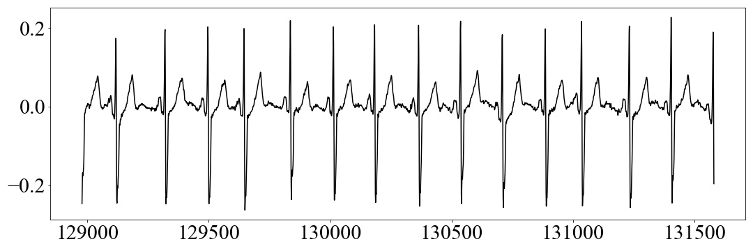
(a) Normal

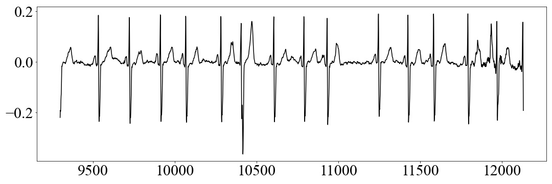
(b) PAF

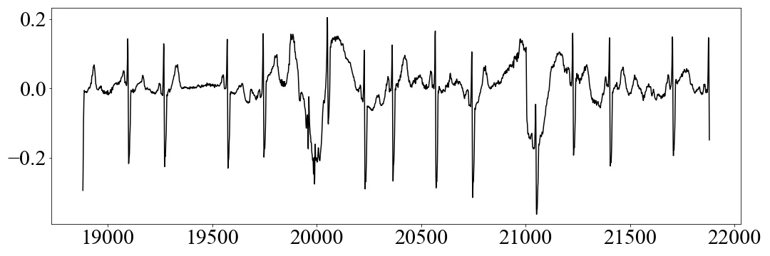
(c) PeAF

Figure 1: Three Category of ECG: Normal, PAF (Paroxysmal Atrial Fibrillation), PeAF (Persistent Atrial Fibrillation).

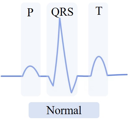
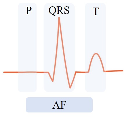
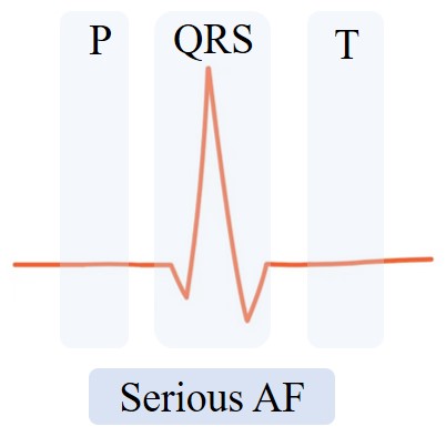
Figure 2: Three types of beat classification: Normal, AF, Serious AF. According to the results of our average waveform experiments, as the risk probability increases, the disappearance of the T wave becomes more pronounced.

Electrocardiogram (ECG) is the most commonly used screening tool for AF, but its effectiveness in early diagnosis is limited [26, 27]. Patients in the early stages are mostly PAF [11]. Most of the time, patients with PAF exhibit sinus rhythm. Existing algorithms can only distinguish between “AF rhythm in AF patients” and “sinus rhythm in normal individuals”, making it challenging to diagnose AF when AF rhythm is absent. Recently, [25, 17]the widespread adoption of wearable devices has increased the likelihood of collecting AF rhythm data through long-term ECG monitoring. However, patients are unlikely to wear these devices continuously due to comfort issues and high costs [23]. Additionally, interpreting this data requires a significant amount of expertise [24]. Therefore, establishing an artificial intelligence (AI) algorithm that identifies “sinus rhythm in AF patients” and “sinus rhythm in normal individuals” is crucial for preventing further complications and avoiding fatalities.

Current research on AF detection during sinus rhythm is limited to segment-level algorithms [12], with no specific algorithms designed for beat-level analysis. The real-life beat waveform is depicted in Figure 2. In this study, we focus on the differences between P waves and T waves. The P wave represents the atrial contraction phase, while the T wave represents the ventricular recovery and repolarization phase [39]. Medical research indicates differences in P-waves between sinus rhythm in AF patients and sinus rhythm in normal individuals [33, 14, 34], highlighting the feasibility of beat-level algorithms. Compared to segment data, beat-level data offers finer granularity, facilitating further analysis of risk variations. Furthermore, beat-level data has lower dimensionality, resulting in lighter models suitable for deployment on portable medical devices. Lastly, with the ability to segment ECG signals, each patient can provide more samples, and decision methods incorporating beat-level information can enhance accuracy.

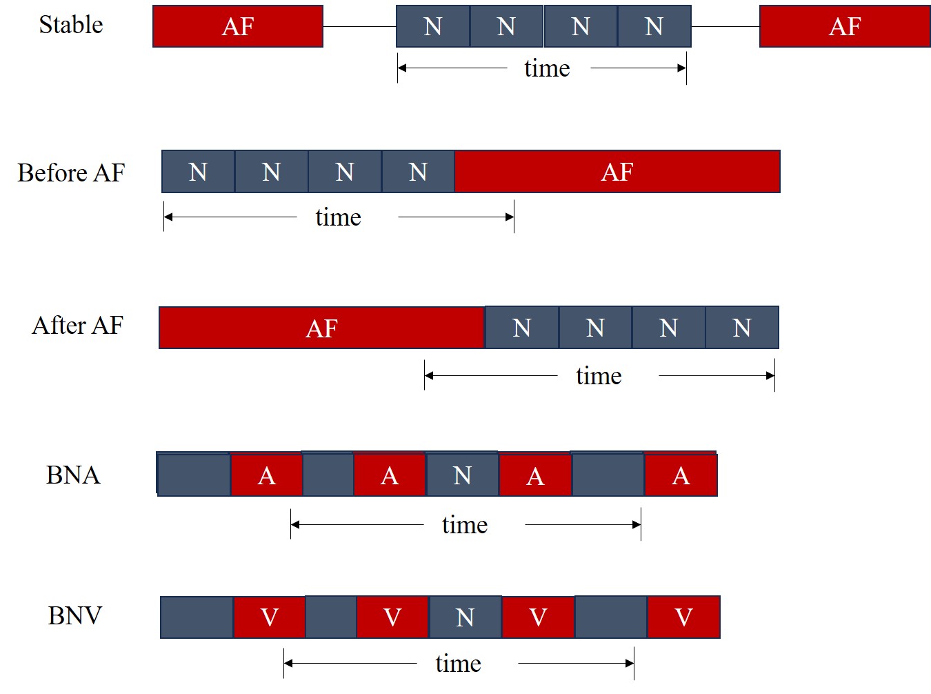
Figure 3: The various partitioning methods for sub-group analysis: Stable, Before AF, After AF, Sinus beat near atrial premature contraction (BNA), Sinus beat near Premature Ventricular Contraction (BNV). The red AF denotes AF segments, the red A represents atrial premature contractions, and the black N represents sinus rhythm.

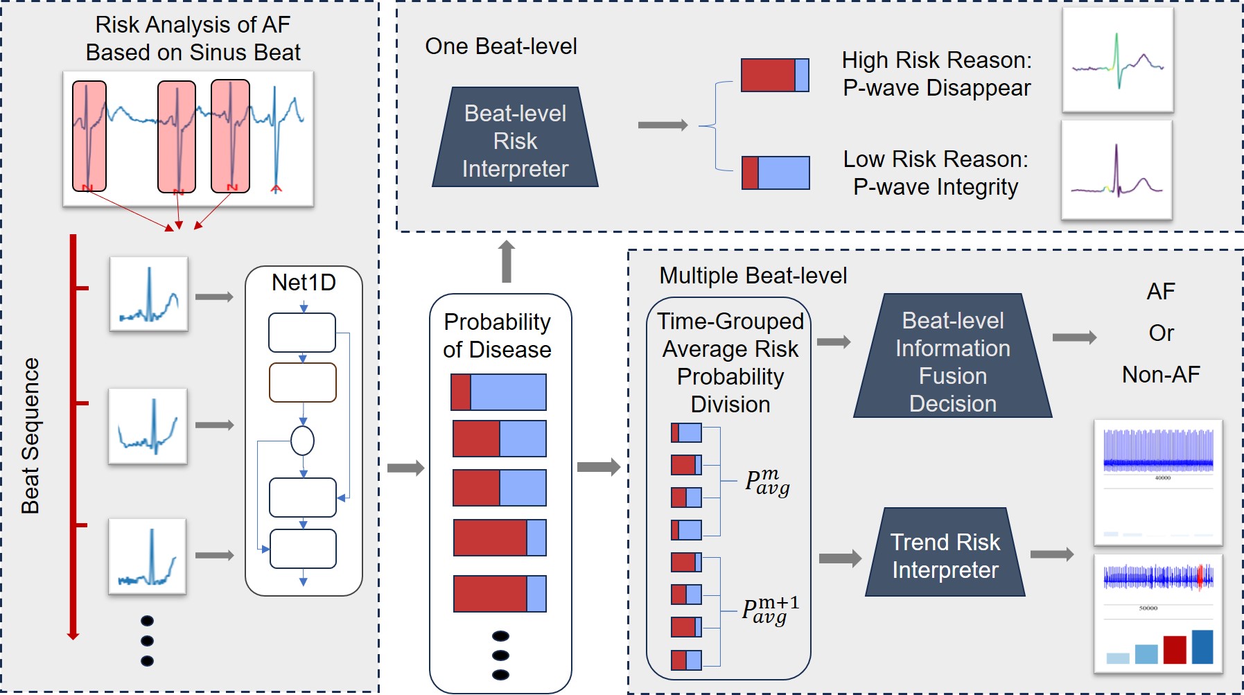
Figure 4: Overview. First, extract sinus beats from the ECG data as the input for Net1d to obtain the probability of being predicted as AF. Depending on the number of beats, two levels of processing can be chosen: for a single beat, the beat-level risk interpreter (BRI) can be used for risk interpretation; when there are a considerable number of beats, the beat-level probabilities are averaged over time groups through Time-Grouped Average Risk Probability Division (TGD), and the beat-level information fusion decision (BID) is employed for AF decision-making; the trend risk interpreter (TRI) is used for trend analysis based on the averaged probabilities over time groups.

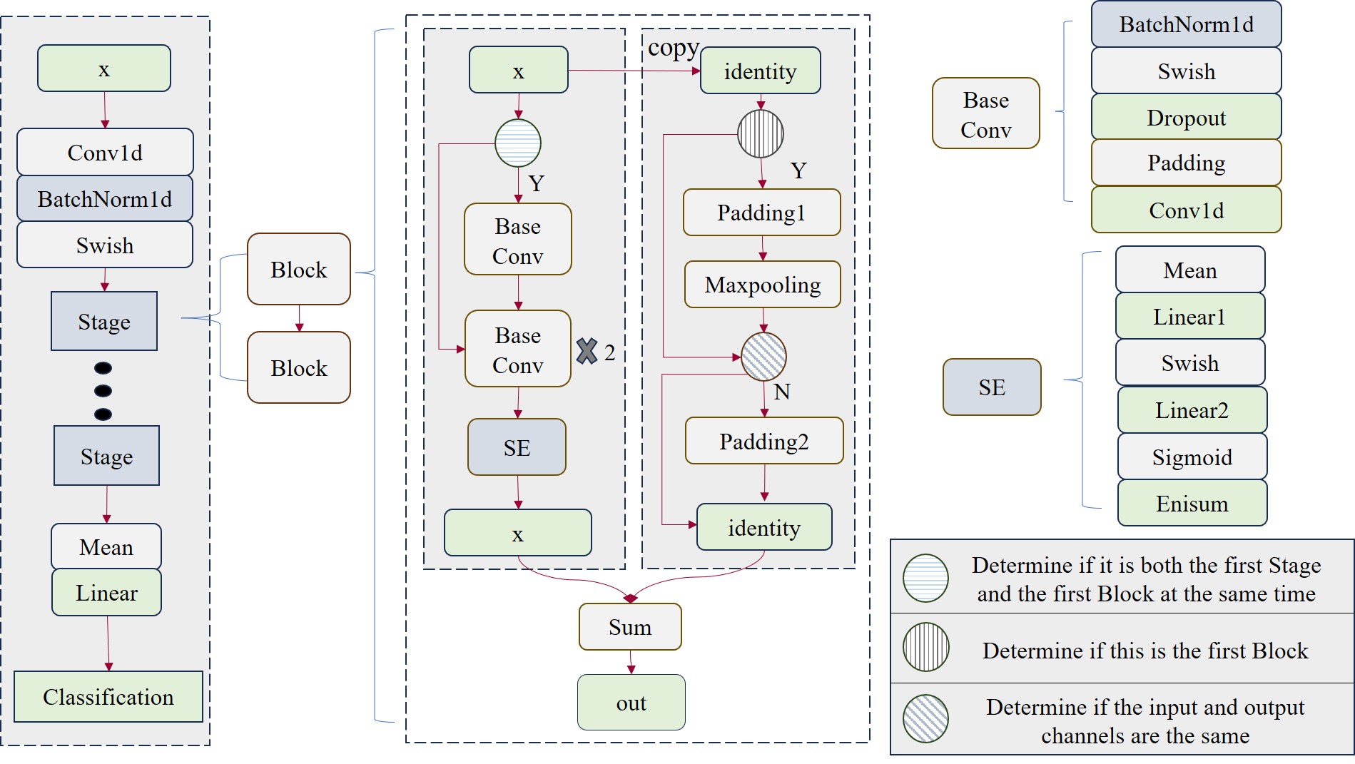
Figure 5: Architecture of Net1d

Addressing the limitations of existing AI algorithms for beat-level AF detection during sinus rhythm, we have identified the following three challenges. First, analyzing beat-level data is more challenging due to lower information content and increased noise during detection. Second, existing algorithms struggle to analyze dynamic changes in patient risk and lack interpretability. Morphological differences in heart rhythms across different stages are minimal, making it challenging to analyze dynamic changes in AF risk. Third, segment-level algorithms are inadequate for considering risk variations, and beat-level studies have been limited to AF segment analysis without considering normal segment data.

In response to the aforementioned challenges, we proposes an interpretable framework for AF risk prediction based on the variation of sinus beat probability. The key contributions of our work are summarized as follows:

• We propose an AF risk analysis algorithm at the beat level to identify “sinus rhythm in AF patients” and “sinus rhythm in normal individuals”. This addresses the issue of diagnosing AF in patients when AF rhythm data is not available. Even in conditions where the majority of data is sinus rhythm, the algorithm can distinguish whether a patient has AF.

• We introduce algorithms such as the beat-level risk interpreter (BRI), beat-level information fusion decision (BID), and trend risk interpreter (TRI), aiding clinicians in providing further explanatory information about a patient’s ECG status during clinical diagnosis. This assists doctors in making accurate decisions. Our algorithms also improve on parameter quantity and computational efficiency, making them more suitable for wearable devices.

• We discover average waveforms for patients at different risk levels and conclude that the higher the risk, the more pronounced the disappearance of the T-wave. We present validation results for different patients using the BRI, TRI algorithms, and experimental results for the BID. In the subgroup analysis, we found that sinus beats near premature ventricular contraction (BNV) have higher predictive value for AF.

2 Related Work

To accurately identify AF from ECGs, various data input forms have been employed for AF detection. Methods for detecting AF in both AF and normal data include using segment-level signals as data input for AF detection, using beat-level signals as data input for AF detection, using a combination of single beat-level and segment-level signals as data input for AF detection. There are also methods focused solely on detecting AF in normal data.

2.1 Detect AF patients during AF rhythm

Segment-level signals as data input

Using segment-level signals as data input for AF detection often involves the application of long short term memory (LSTM) deep learning models and convolutional neural network (CNN)[2, 3, 4, 29, 5, 6, 7, 8, 35]. In [2], a combination of CNN and LSTM model is employed to detect waveforms of different heartbeat signals, eliminating the need for feature engineering. While achieving high sensitivity, there is still potential to enhance the capability of filtering AF from other cardiac rhythms. On the other hand, [3] demonstrates the ability to update model parameters and accurately predict AF with different duration and lead distributions, showing better performance in identifying AF from other rhythms. In [8], a combination of AF rhythm and morphological information improves the accuracy of AF detection, and the algorithm exhibits strong interpretability. However, there is room for improvement in discerning AF from uncertain ECG signals where P-waves may be obscured by noise.

Beat-level signal as data input

Using beat-level signals as input for AF detection has been explored in [9]. In [9], a CNN was employed to automatically recognize and classify five different types of heartbeats in ECG signals, including normal (N), supraventricular ectopic (S), ventricular ectopic (V), fusion (F), and unknown (Q) heartbeats. This approach, compared to traditional machine learning methods, has the advantage of automatically learning features from ECG signals without the need for manually designed feature extractors. The paper also addressed the issue of class imbalance in the dataset by using synthetic data to balance the categories of heartbeat data.

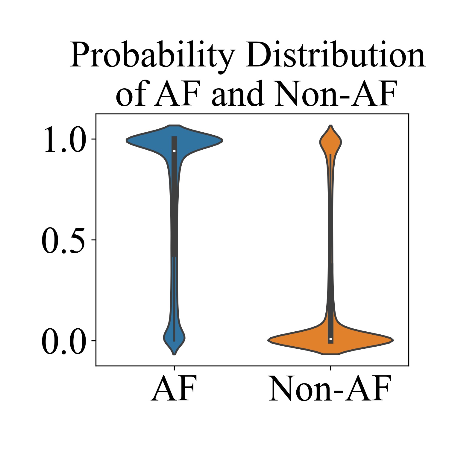
(a)

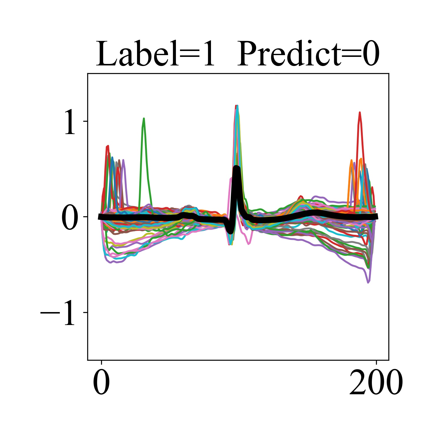
(b)

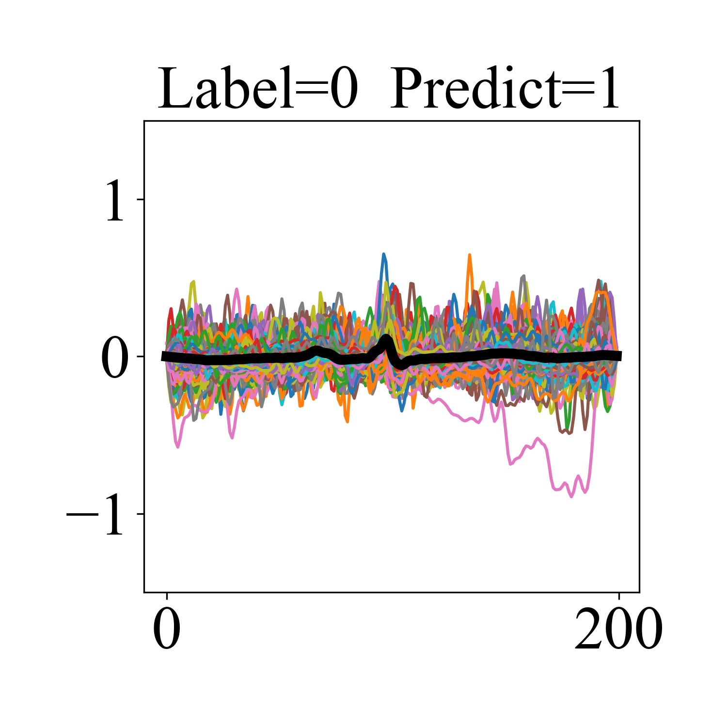
(c)

(d)

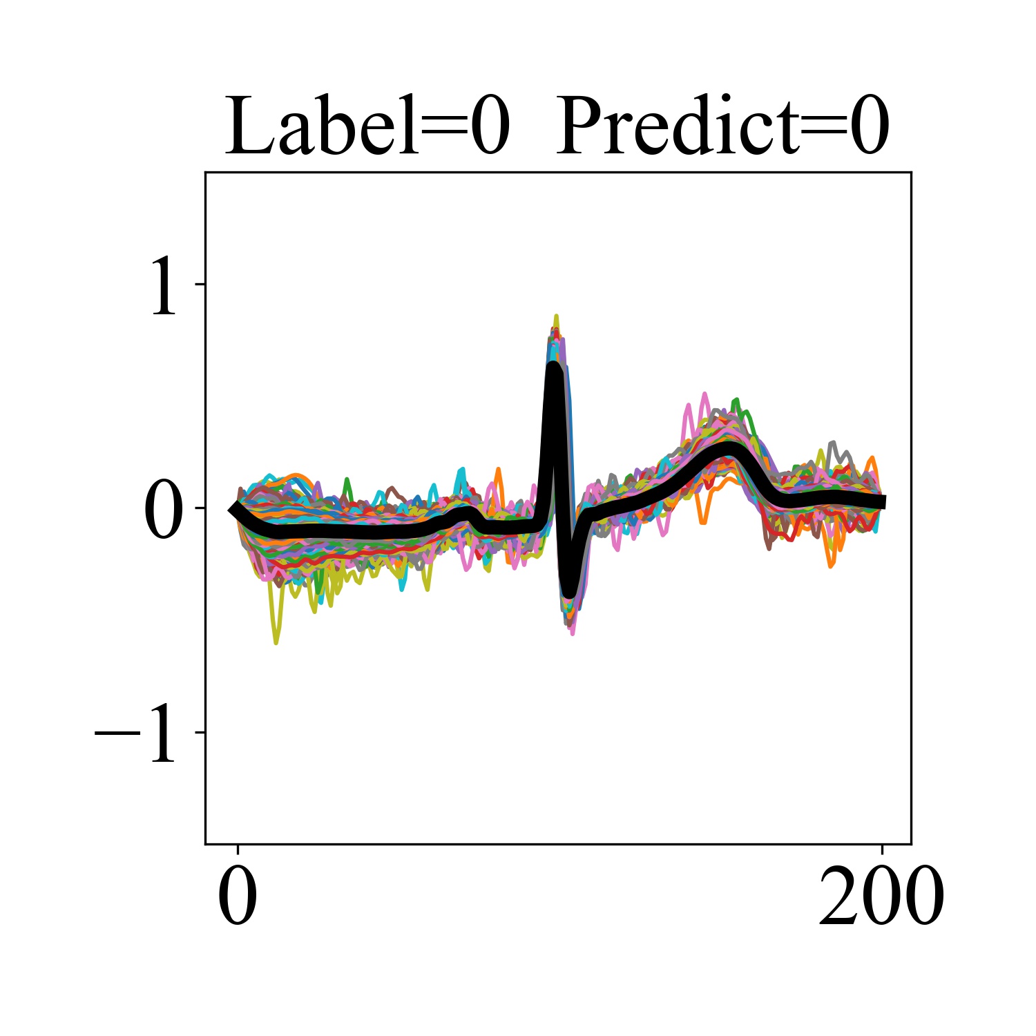
(e)

Figure 6: Variations in model prediction probabilities. (a) The horizontal axis represents the groundtruth of the samples (AF or non-AF), while the vertical axis represents the probability assigned by the model for each sample to be AF. The width of the graph represents the relative density of the sample count corresponding to the current probability. (b) & (c) Illustrate the shapes of samples where the model predicted incorrectly for AF and non-AF labels. The horizontal axis represents the data points of a beat (fixed at 200), and the vertical axis represents the filtered beat values. The bold black waveform represents the result of averaging the values (d) & (e) Illustrate the shapes of samples where the model predicted correctly for AF and non-AF labels.

Beat-level and segment-level signals combined as data inputs

Using a combination of beat-level and segment-level signals as input for AF detection has been explored in studies such as [16] and [20]. In [16], MINA combines CNN and bidirectional Long Short-Term Memory network (Bi-LSTM) to extract domain-specific features at different levels (beat-level, rhythm-level, and frequency-level). These features are then combined with ECG data, and a multi-level attention model is employed to enhance the interpretability of the model. This allows the model to identify key beat positions, significant rhythm variations, and important frequency components in ECG signals. [20] proposes a novel two-step approach for detecting AF events. The first step involves using a Support Vector Machine (SVM) to classify the rhythm type of ECG signals into three categories: non-AF, PAF, and PeAF. The second step utilizes a CNN model to classify heartbeats predicted as AF rhythms, determining the onset and offset points of AF events.

2.2 Detect AF patients during sinus rhythm

Detection of AF using solely normal ECG signals as data input [12]. [12] employed a ResNet architecture to identify ECG features indicative of AF during sinus rhythm. The study designed a method for data collection in interest windows for AF and non-AF patients, allowing the model to distinguish between the sinus rhythm of AF and non-AF patients. However, the collection method may introduce errors, and the discrete nature of temporal sampling could lead to misclassification of certain patients.

In the four data input forms mentioned for AF detection, none have utilized beat-level sinus rhythm heartbeats as input data. Patients with PAF often exhibit subtle symptoms in the early stages. Therefore, analyzing abnormal signs in sinus rhythm heartbeats in ECG is crucial for preventing AF. Furthermore, comparison with widely used segment-level signal data reveals that beat prediction probabilities fluctuate with the emergence of AF segments. This indicates that beat-level data exhibits higher sensitivity for AF alerts, enabling timely diagnosis and treatment for patients.

3 Methods

In this section, we initially define the problem under consideration and subsequently offer an overview of the algorithmic process. Following this, we provide a detailed explanation of the Risk Analysis of AF Based on Sinus Beat. After obtaining the probability of disease for each beat, we can opt for the One Beat-level module, employing BRI for individual beat risk interpretation. Alternatively, the Multiple Beat-level module can be selected to derive the average risk probability through Time-grouped average risk probability division (TGD). Finally, the BID is utilized for AF decision-making, while the TRI serves as a tool for interpreting risk trends. Our code is publicly available at https://github.com/leijsen/ECGBeat4AFSinus

3.1 Problem definition

A patient has multiple diagnostic segments of ECG denoted as $S_{i},i\leq K$, where $K$ represents the number of segments the patient has. Each segment is a two-lead ECG data $X\in\mathbb{R}^{2\times N}$, where $N$ represents the length of each lead signal. Initially, we obtain data for a single lead of the patient’s ECG, denoted as $x\in\mathbb{R}^{1\times k}$, where $k$ is the number of R-peaks in a lead signal. Based on the doctor’s localization of R-peaks and a sampling rate of 200 Hz, we obtain beat-level data $d$, corresponding to one heartbeat. Simultaneously, based on the doctor’s classification of each beat, we filter out beats labeled as ‘N’. Given the data for a sinus beat $d$, our risk analysis task is to output a binary label $Y\in\{0,1\}$, indicating whether the corresponding beat data is non-AF or an AF segment, along with the risk probability $p\in[0,1]$.

Index	Accuracy	Recall	Precision	F1	AUC
1	0.5581	0.5778	0.4836	0.5265	0.5845
2	0.6093	0.6713	0.5426	0.6001	0.6737
3	0.7438	0.7240	0.6693	0.6956	0.8129
4	0.7520	0.7263	0.7630	0.7442	0.8334
5	0.6399	0.5662	0.8155	0.6684	0.7527
Avg	0.6606	0.6531	0.6548	0.6470	0.7314

Table 1: Cross-validation results. The indices below represent the test set names for the 5 cross-validation experiments and the averaged results after experiments.

We define a continuous time series probability $P=\{p_{1},p_{2},\cdots,p_{i},p_{i+1},\cdots,p_{j},p_{j+1},\cdots,p_{k}\}$, where $n=j-i+1$, and $n$ is the number of beats in a time group, $1\leq n\leq k$. The average risk probability for the $m$-th time group is denoted as $P_{avg}^{m}$, where $m\in\{1,2,\cdots,\lceil\frac{k}{n}\rceil\}$. For a continuous sequence of $t$ average risk probabilities $\{P_{avg}^{1},P_{avg}^{2},\cdots,P_{avg}^{t}\}$, we can interpret the reasons for its variation, providing specific locations of abnormal ECG features and the level of AF risk. The overall variable explanations are provided in table 2.

3.2 Overview

As shown in Figure 4, the three main modules include: 1) AF risk analysis algorithm based on sinus beats, predicting AF for unknown patients’ sinus beats; 2) The One Beat-level module includes BRI: providing interpretable analysis for individual sinus beats; 3) The Multiplt-level module includes TGD, BID and TRI. TGD: segmenting continuous individual beat probabilities into time groups and calculating the average risk probability within each group; BID: fusing information across a group of beats to improve diagnostic accuracy; TRI: explaining the dynamic changes in patient risk. Depending on the amount of input data, different modules are utilized to perform targeted analyses on the data.

During the training phase, we construct a beat sequence using segmented sinus beats and sequentially input them into the Net1D model. In the testing phase, given multiple beat data $D=\{d_{1},d_{2},\cdots,d_{i}\}$ for a patient, we input it into the trained model to obtain the predicted probabilities for the data $D$, denoted as $P=\{p_{1},p_{2},\cdots,p_{i}\}$. BRI, located in the upper right corner of Figure 4, provides the risk interpretation for individual sinus beats. After TGD, $P$ is transformed into $P_{avg}=\{P_{avg}^{1},P_{avg}^{2},\cdots,P_{avg}^{t}\}$. BID, located in the middle right of Figure 4, offers a more accurate AF diagnosis for $P_{avg}$. TRI, located in the bottom right of Figure 4, provides interpretable risk change analysis for $P_{avg}$.

Symbol	Definition
$S$	ECG diagnostic segment
$K$	Number of segments a patient
$X\in\mathbb{R}^{2\times N}$	Dual-lead ECG data
$N$	Number of ECG data points
$x\in\mathbb{R}^{1\times N}$	Data from a single lead
$k$	Number of beats in a lead
$d$	Data of a heartbeat
$Y$	Binary label
$p$	Risk probability
$P=\{p_{1},p_{2},\cdots\}$	Sequential risk probability
$n$	Number of beats in a group
$P_{avg}^{m}$	Average risk probability
$m$	Present time group
$t$	Continuous t time groups
$P_{avg}=\{P_{avg}^{1},\cdots\}$	Average sequence
$Rloc$	R-peak localization
$Rclas$	Beat classification
$L$	Length of a beat
$l$	Left index of a beat
$r$	Right index of a beat
$D=\{d_{1},d_{2},\cdots\}$	Heartbeat data of a patient
$L_{y,p}$	Model loss function
$\alpha$	Left index of the time group
$\beta$	Right index of the time group
$layer$	Output layer
$f_{l}$	Function of the $l$-th layer
$\theta_{l}$	Parameters of the $l$-th layer
$v$	Feature map value
$f$	Foward propagation function
$w$	Output layer weights
$cam$	Class activation map
$map$	Mapped result
$pre$	Predicted label
$threshold$	Risk threshold

Table 2: Table of symbols

3.3 Risk Analysis of AF Based on Sinus Beat

Firstly, we preprocess the selected dataset, including necessary filtering steps to eliminate baseline drift and optimize signal quality, preventing shortcut issues [1]. Based on the doctors’ localization of the R-peaks in the dataset, denoted as $Rloc$, where $Rloc[i]$ represents the time scale of the R-peak for the $i$-th heartbeat in the entire ECG, $1\leq i\leq k$. According to the doctors’ labels for each beat in the dataset, denoted as $Rclas$, beats are periodic metadata in the ECG, where $Rclas[i]$ indicates the type of the $i$-th beat, $1\leq i\leq k$. With a sampling rate of 200Hz, we define the length $L$ of a beat as 200. For the $i$-th beat, we define its left index $l_{i}$ and right index $r_{i}$ using equation:

$$l_{i}=Rloc[i]-\frac{L}{2},\quad r_{i}=Rloc[i]+\frac{L}{2}$$ (1)

All data in a single lead is segmented into beat-level data sequences of equal length, denoted as $D=\{d_{1},d_{2},\cdots,d_{k}\}$. The segmentation starts from the 10-th R-peak and continues until the 5-th R-peak from the end to avoid noise at the beginning and end of data collection. Based on $Rclas$, each beat is classified as either ‘N’ or non-‘N’. ‘N’-type beats are retained, while non-‘N’-type beats are discarded, resulting in all sinus rhythm data for a patient. Since we are analyzing a binary classification problem, if a patient has at least one segment $S_{i}$ marked as abnormal by doctor, the labels for all heartbeat segments $\{S_{1},S_{2},\cdots,S_{K}\}$ for that patient, as well as the label for the beat data sequence $D$ within each segment, are defined as 1. Abnormal segments include PAF or PeAF. Otherwise, all heartbeat data $D$ is defined as 0.

After segmenting the ECG signals into beats, we use the Net1d model [32] with sinus beat data $d$ as input to learn implicit AF risk information in sinus data and determine if the subject has AF. Figure 5 illustrates the architecture of the Net1d model, detailed as follows.

Net1D first performs feature extraction on the data, consisting of conv layers, BatchNorm (BN), and swish activation layers. There are 7 different-shaped stage modules, followed by averaging and linear layers to obtain probabilities for predicting 0 and 1.

Each stage module contains 2 block layers, and a block layer is generally composed of 3 decision points, a baseConv layer, and a SqueezeAndExcitation (SE) layer. The 3 decision points are: checking if this block belongs to both the first stage and the first block, if so, the input goes through the first baseconv layer and then the following two baseconv layers; checking if this block belongs to the first block, in which case, intermediate data goes through padding and maxpool layers; checking if the dimensions of input and output channels are the same, if not, the data goes through another padding layer. Note: the two padding layers have some differences in their processing. The final output is obtained by using the Sum function.

The specific baseConv layer is composed of BN layer, swish activation layer, dropout layer, padding layer, and conv layer. The detailed SE is composed of averaging layer, linear layer, swish activation layer, linear layer, sigmoid layer, and the enisum layer, defined as follows: considering two matrices, one with dimensions $(a,b,c)$, and the other with dimensions $(a,b)$. Their multiplication, represented by the Einstein summation convention, is given by the formula (2).

$$A_{a*b*c}=B_{a*b*c}\cdot C_{a*b}$$ (2)

Where $A,B,C$ represent matrices, and $a$, $b$, and $c$ are the dimensions of the first matrix, and $a,b$ are the dimensions of the second matrix.

The cross-entropy loss function $L_{y,p}$ for the model is given by:

$$L_{y,p}=-\left(y\cdot\log(p)+(1-y)\cdot\log(1-p)\right)$$ (3)

where $y$ represents the real label, $p$ represents the predict label.

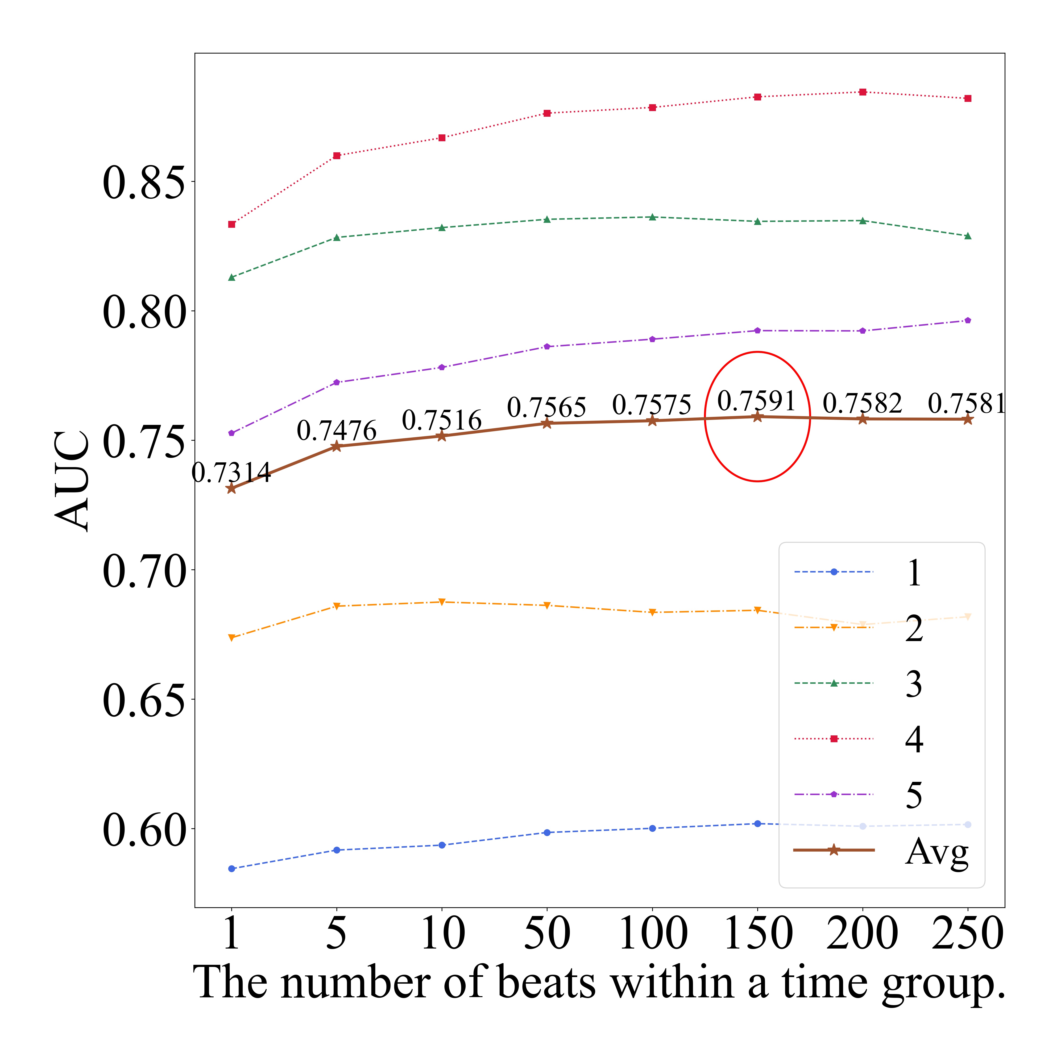
Figure 7: Performance of the beat-level information fusion decision (BID) algorithm. The horizontal axis represents the number of beats in a time group, denoted as $n$. The vertical axis represents the AUC value. Labels indicate different indices corresponding to the index.

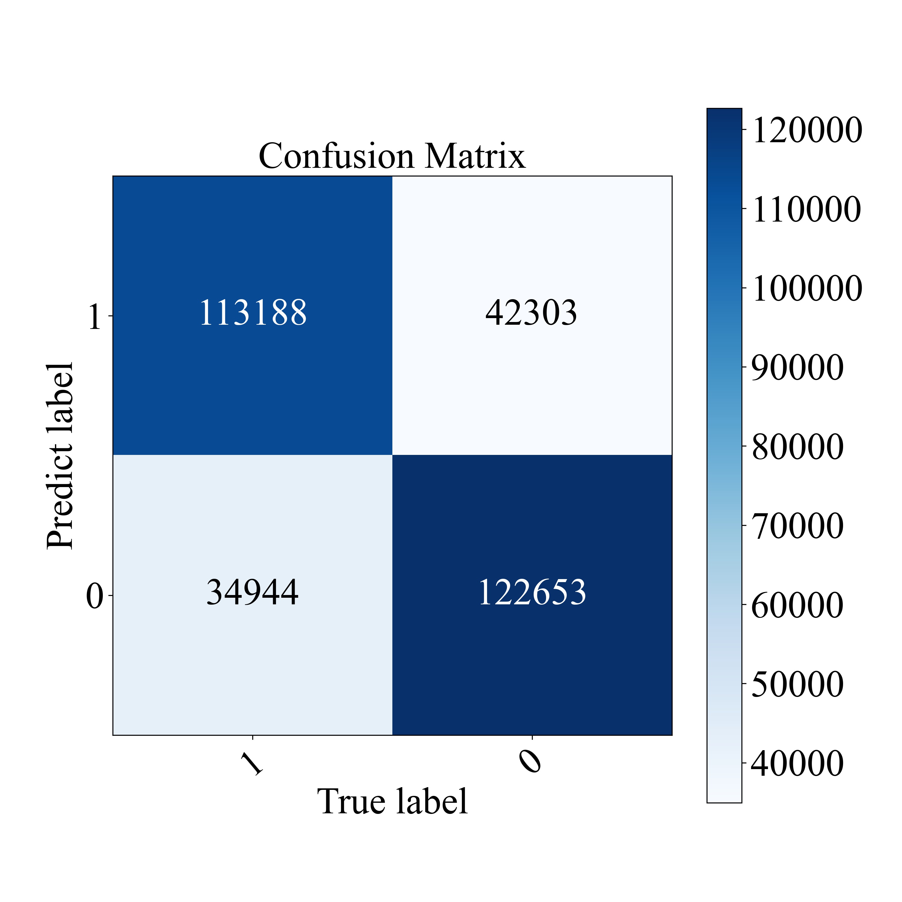
Figure 8: Confusion matrix.

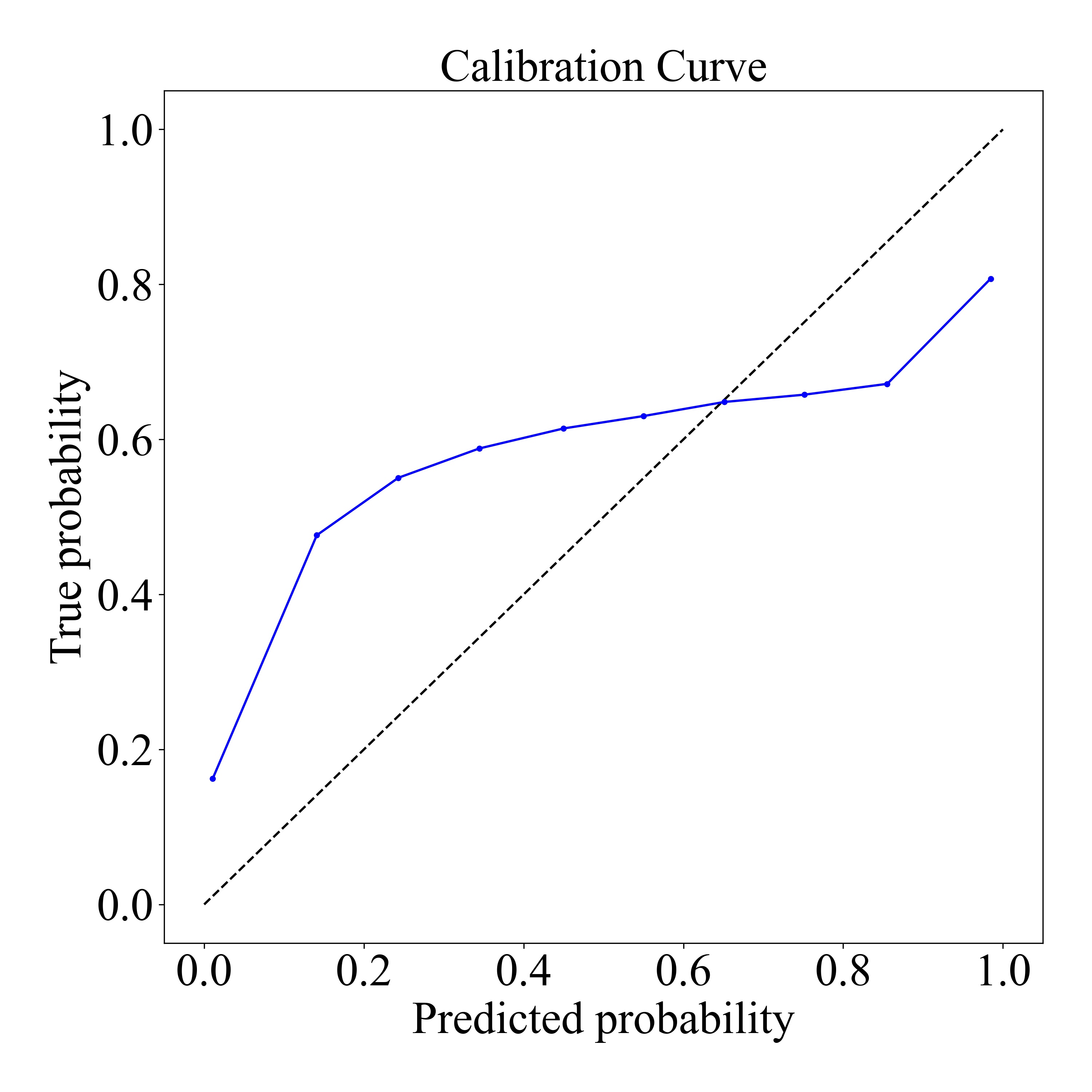
Figure 9: Calibration Curve for AF. The fitted calibration curve illustrates the relationship between the model-predicted probability of a sample being AF (x-axis) and the actual probability of the sample being AF (y-axis).

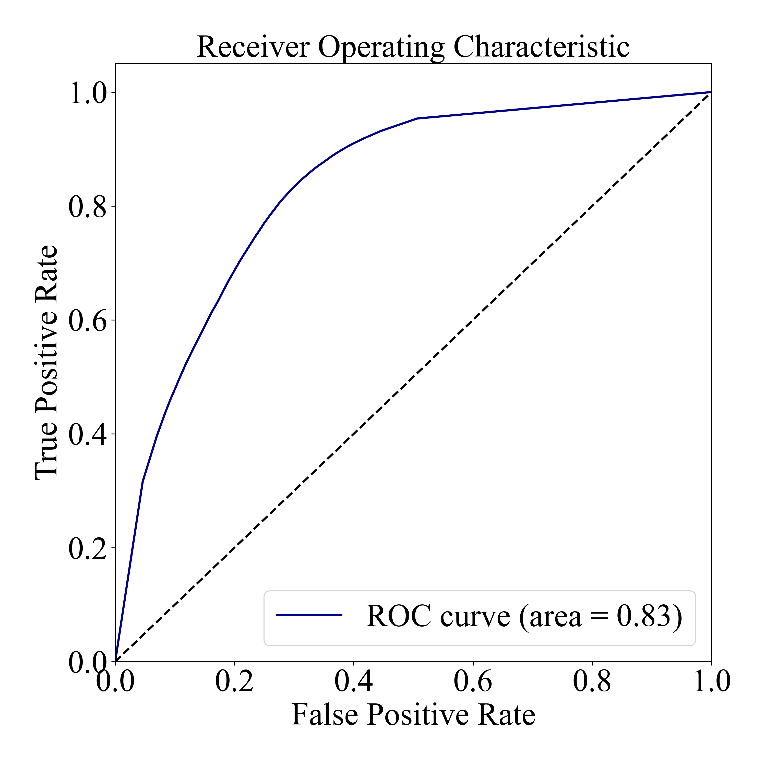
Figure 10: ROC-AUC Curve.

Figure 11: T-SNE Clustering of Images. Represents the dimensionality reduction results after classification using the model.

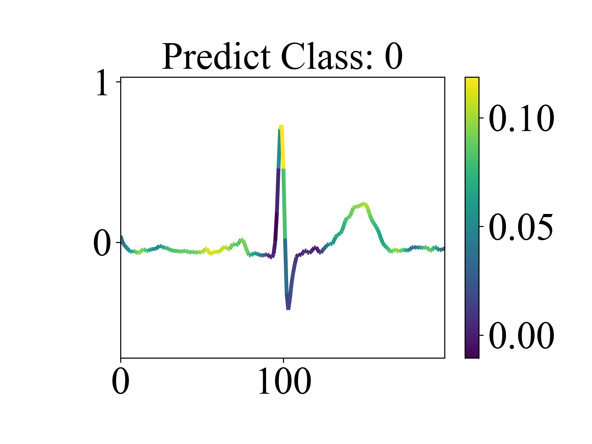
(a)

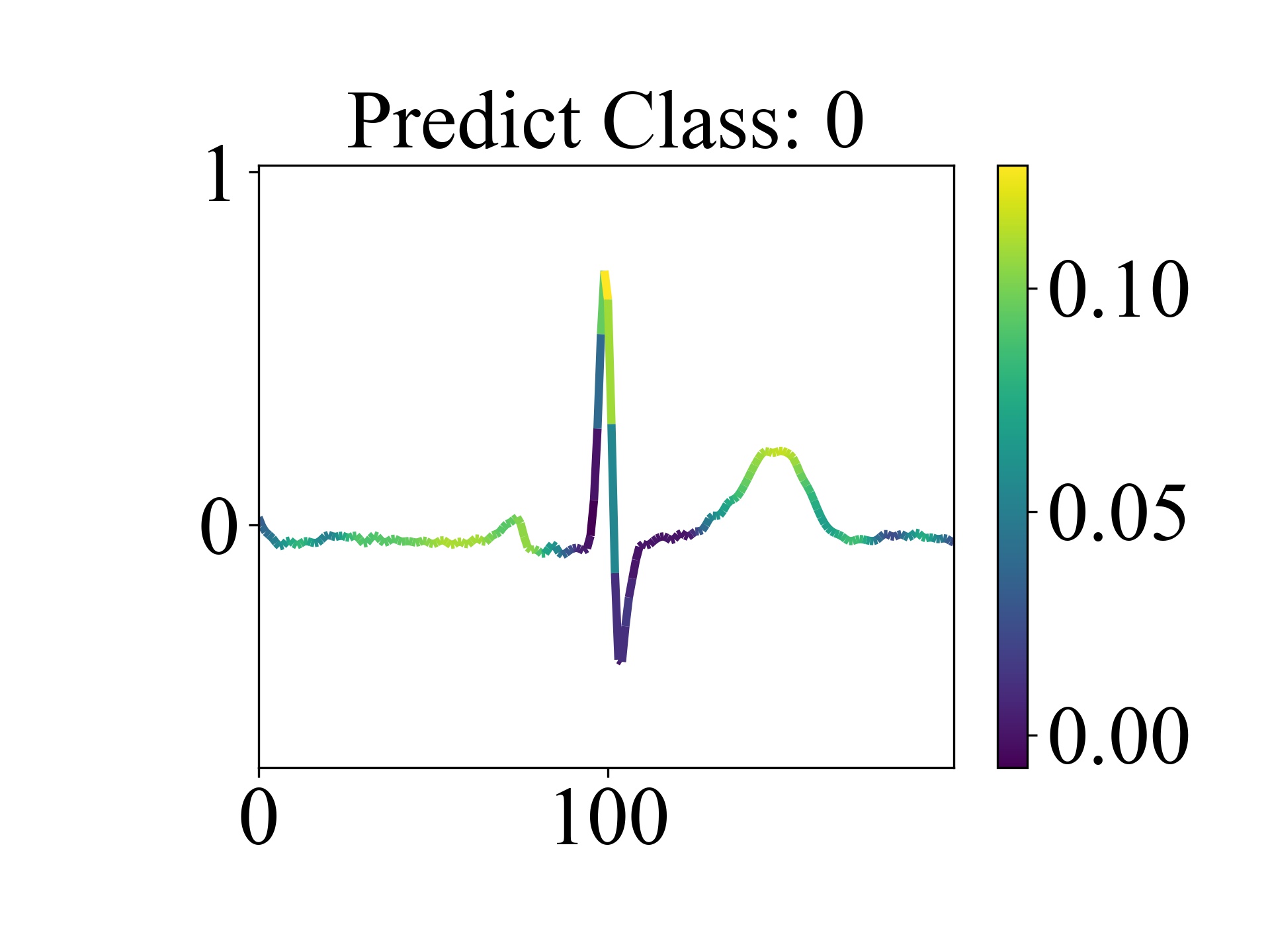
(b)

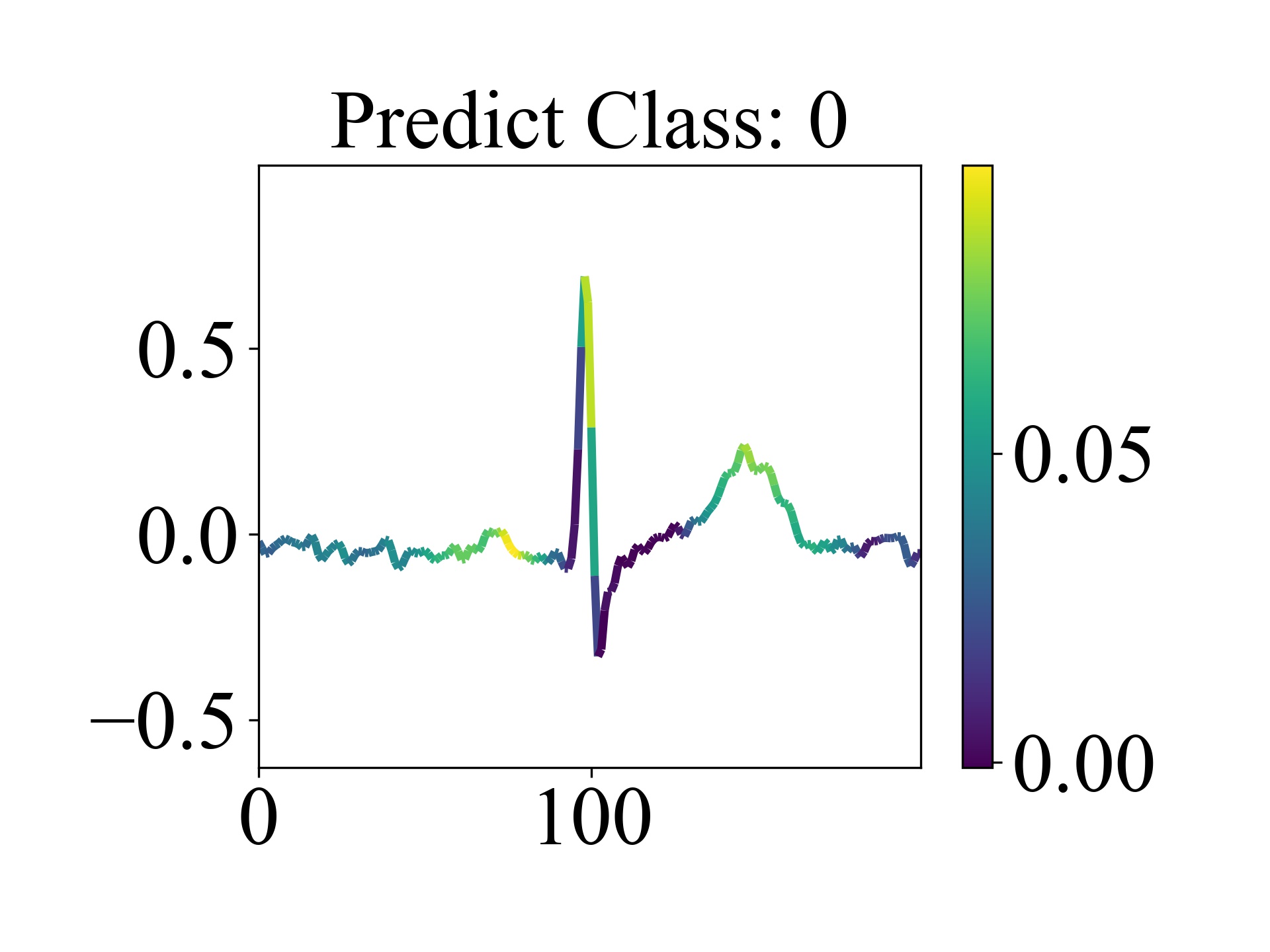
(c)

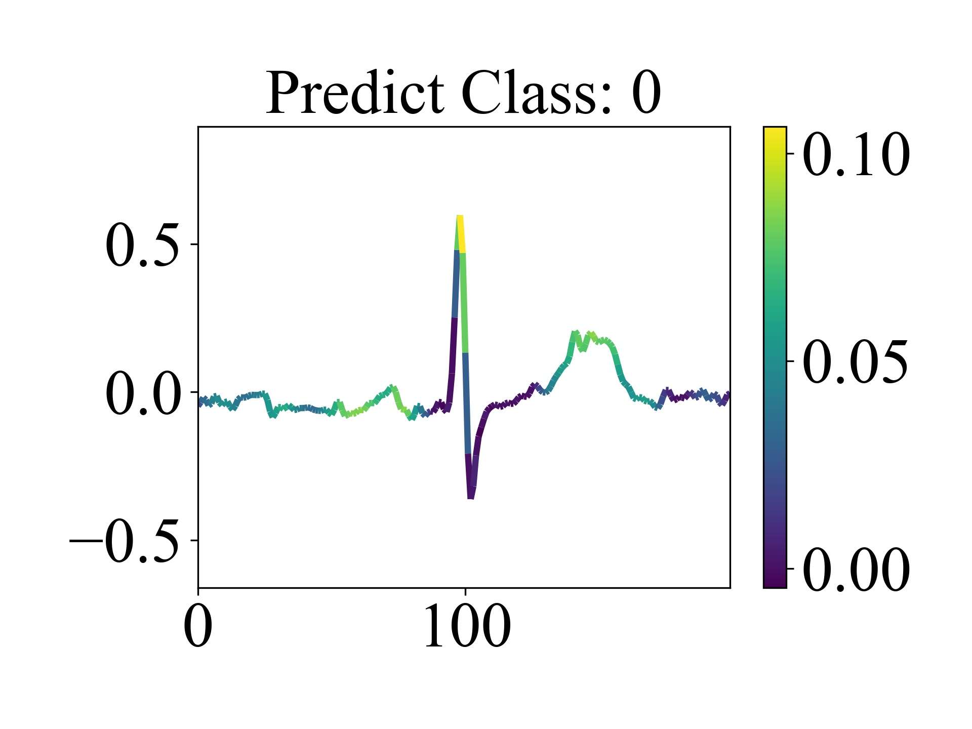
(d)

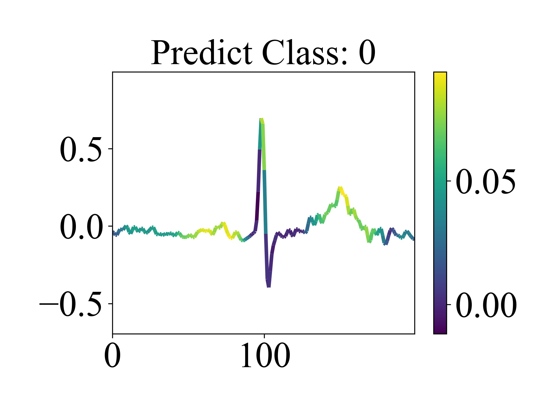
(e)

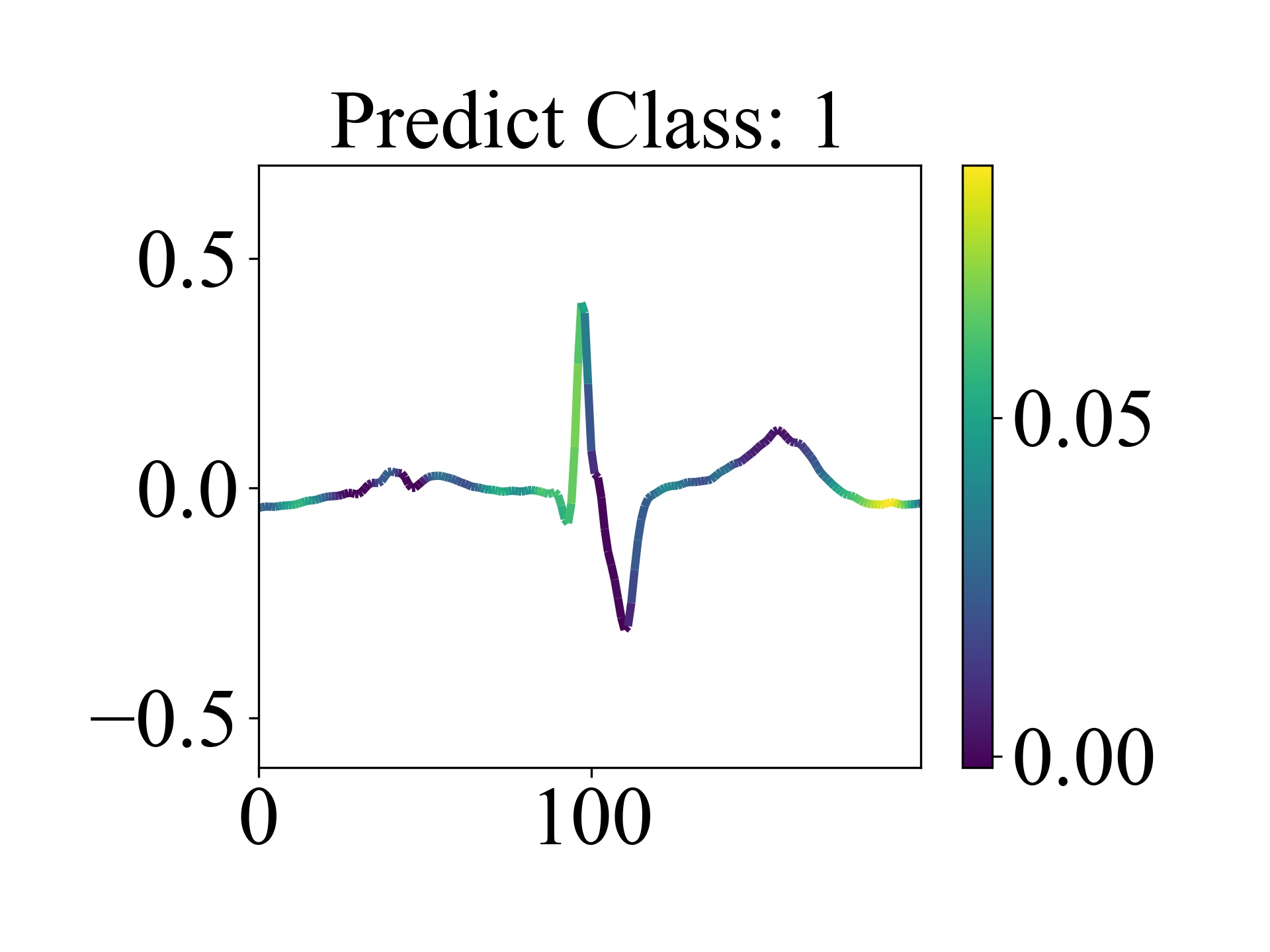
(f)

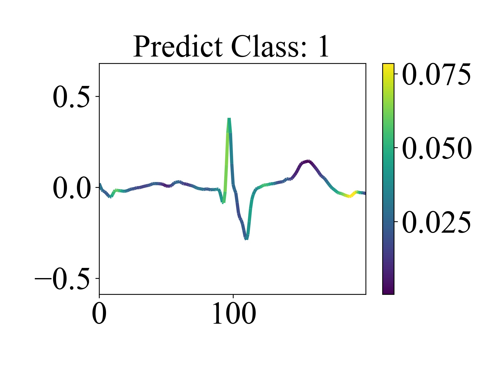
(g)

(h)

(i)

(j)

Figure 12: The image of CAM. The images (a)-(e) in the upper section represent normal sinus beats in healthy individuals, while the images (f)-(j) in the lower section represent sinus beats in patients with AF.

3.4 One Beat-level Module

Beat-level Risk Interpreter

In clinical judgment, physicians often focus on the pathological regions of beats [31]. Therefore, we utilize the Class Activation Map (CAM) method to visualize and interpret the model’s output. The CAM method highlights which parts of the beat data contribute more to the prediction output. Higher scores result in more vibrant colors, indicating a higher importance of each region for the predicted category. As illustrated in Figure 4 on the upper right, brighter areas suggest that the model pays more attention to those regions, providing guidance on why the model predicts a particular beat as AF or non-AF. The detailed process is as follows:

$$layer=f_{l}(d;\theta_{l})$$ (4)

$layer$ represents the model’s output layer, $f_{l}$ represents the forward propagation function of the $l$-th layer of the model, $d$ represents the input beat-level data, and $\theta_{l}$ represents the parameters of the $l$-th layer of the model.

$$v=f(d;layer)$$ (5)

$v$ represents the feature map value, and $f$ denotes the forward propagation function of the model.

$$w=\frac{\partial L_{y,p}}{\partial layer}$$ (6)

$w$ represent the weights of the output layer, and $L_{y,p}$ denotes the loss function.

$$cam=v\cdot w$$ (7)

$cam$ represents the class activation map.

$$map=ReLU(\sum_{i=1}^{n}cam_{i})$$ (8)

$map$ represents the result after mapping the class activation map, $\sum_{i=1}^{n}cam_{i}$ represents the summation across the first dimension of $cam$.

3.5 Multiple Beat-level Module

Time-Grouped Average Risk Probability Division

Given a patient’s beat sequence $D$, we obtain the model Net1d’s predicted risk probability sequence $P=\{p_{1},p_{2},\cdots,p_{k}\}$, where $k$ is the number of beats in the sequence $D$. We divide $n$ consecutive beats into a time group, and the average risk probability $P_{avg}^{m}$ for the $m$-th time group is calculated as follows:

$$P_{avg}^{m}=\frac{\sum_{i=\alpha}^{\beta}p_{i}}{n}$$ (9)

Here, $\alpha$ represents the left index of the $n$ consecutive beats, $\beta$ represents the right index, and $m$ is the index of the current time group. After calculating the average risk probability for each time group, we form the sequence of time group average risk probabilities $P_{avg}=\{P_{avg}^{1},P_{avg}^{2},\cdots,P_{avg}^{t}\}$, $t=\lceil\frac{k}{n}\rceil$.

Beat-level Information Fusion Decision

In clinical practice, making a diagnosis based on a single beat-level data may have some randomness. Therefore, leveraging the flexibility and granularity advantages of beat-level data, we propose the BID algorithm. It is described as follows:

We take the average of the predicted probabilities of $n$ consecutive beats for a patient, denoted as $P_{avg}^{m}$, as the average risk probability for this segment of data. When the average risk probability exceeds a certain threshold, it indicates that the patient has a high probability of having AF.

$$\text{pre}=\begin{cases}1&\text{if }p_{avg}^{m}\geq threshold\\ 0&\text{if }p_{avg}^{m}<threshold\end{cases}$$ (10)

Where $pre$ represents the predicted label for the patient, with 1 indicating AF and 0 indicating non-AF. $threshold$ denotes the risk threshold defined by the doctor, with $0\leq threshold\leq 1$, and the risk threshold can be adjusted according to the actual situation.

Trend Risk Interpreter

In clinical diagnosis, medical practitioners focus extensively on segments displaying abnormal beats, facilitating a thorough analysis of these anomalous cardiac rhythms. Following the acquisition of a sequence of average risk probabilities $P_{avg}$, we undertake an adjusted examination of this $P_{avg}$ sequence to observe the trend of risk variations, as depicted in the lower right corner of Figure 4. During testing, when $P_{avg}^{m}$ falls outside an AF segment, it is depicted in blue. The intensity of blue signifies a higher risk value of $P_{avg}^{m}$, with deeper shades indicating increased risk. Conversely, when $P_{avg}^{m}$ corresponds to an AF segment, it is depicted in red. In normal ECG, each $P_{avg}^{m}$ value typically remains below the risk threshold $threshold$ and exhibits a stable trend, signifying a low likelihood of abnormality in this beat segment. In contrast, for ECGs of AF patients, $P_{avg}^{m}$ demonstrates an ascending trend from normal to AF segments, indicating a heightened probability of abnormality in this segment.

4 Experiments and results

In this section, we will first introduce the dataset used, then describe the performance of the model. We will showcase the results of subgroup analysis, comparing the parameters count of models at different levels. Finally, we will highlight interpretability and new discoveries. We primarily utilize the model with index=4 to showcase the results of various experiments.

4.1 Dataset

This study utilized publicly available datasets provided by CPSC 2021, accessible at [38]. These databases consist of 1436 ECG recordings from 105 subjects, selected from the I-lead and II-lead of long-term dynamic ECG signals. In this paper, only the data from the I-lead was used. The duration of the records varies, ranging from 0.14 to 411.11 minutes, with an average duration of 20.33 minutes [20]. All records have an original sampling rate of 200 Hz.

In terms of data processing, this study employed a specific method to label patients with AF. Specifically, if there is at least one instance of AF in the data segment for a given patient, the entire patient is labeled as having AF. Following this classification criterion, a total of 54 subjects were marked as having AF, while the remaining 51 were classified as non-AF patients. This classification was implemented to ensure the accuracy of the model in detecting patients with AF and to enhance the model’s sensitivity to AF data.

Additionally, we segmented approximately 21,469,915 heartbeats from these records, including 888,067 AF-related data and 1,258,848 normal heartbeat data.

(a)

(b)

Figure 13: Temporal Changes in Average Risk Probability. In Each Subplot, the upper panel depicts an ECG waveform, where the blue segments represent normal periods, and the red segments indicate AF episodes. The lower panel illustrates the time-averaged risk probability values, with blue denoting normal segments and red indicating AF segments. Each group consists of 20 beats.

4.2 Classification performance

We evaluate the model performance using key performance metrics including accuracy, precision, recall, and Area Under Curve (AUC). The results of the 5-fold cross-validation are shown in Table 1. We choose the model with index=4 for displaying the AUC plot in Figure 10. The BID enhances the precision of patient prediction, as depicted in Figure 7, illustrating the variation of AUC values with different lengths of time group within beat quantity $n$. The graph indicates that as $n$ increases, the AUC value tends to grow, especially in the range from 1 to 10, showing a noticeable improvement. It is evident that, with the assistance of the BID algorithm, beat-level risk assessment can enhance accuracy. When there is a relatively larger number of beats, a higher level of detection can be achieved. However, when the number of heartbeats increases to a certain threshold, further increases can lead to a decrease in results.

We designed Figure 6 to showcase the probability distribution of model outputs. It illustrates the confidence of the model on different samples and reveals the uncertainty of the model across different categories. By presenting multiple data points and their corresponding average waveforms, we demonstrate both samples predicted incorrectly and those predicted correctly by the model, along with their approximate shapes. The experiment confirms that the majority of beat data is correctly classified. However, there is a small portion that is misclassified, such as beats from AF patients being classified as normal. This misclassification may occur when certain key features of the beat, such as the P-wave or T-wave, have minor fluctuations, misleading the model into thinking it belongs to a normal individual. Similarly, some beats from normal individuals may be misclassified as AF. This could be attributed to the prominent P-wave features of the beat but with a partial disappearance of the T-wave, leading to misclassification.

We conducted a detailed analysis of the model’s classification results through the confusion matrix shown in Figure 8. This matrix visually displays the model’s performance on true positives, false positives, true negatives, and false negatives. The darker the values on the main diagonal, the higher the probability that the model predicted correctly.

In order to further evaluate the calibration performance of the model, we plotted the calibration curve shown in Figure 9. This curve illustrates the accuracy of the model’s probability predictions. From the curve, it can be observed that the model predictions are overly confident, with predicted probabilities tending to be either 0 or 1, resulting in an inverted sigmoid shape for the blue curve.

Through the T-SNE clustering analysis in Figure 11, we observed the distinctiveness of the model. After the model distinguishes the data, there is a clear separation, proving that the model has a certain ability to differentiate between data with different labels.

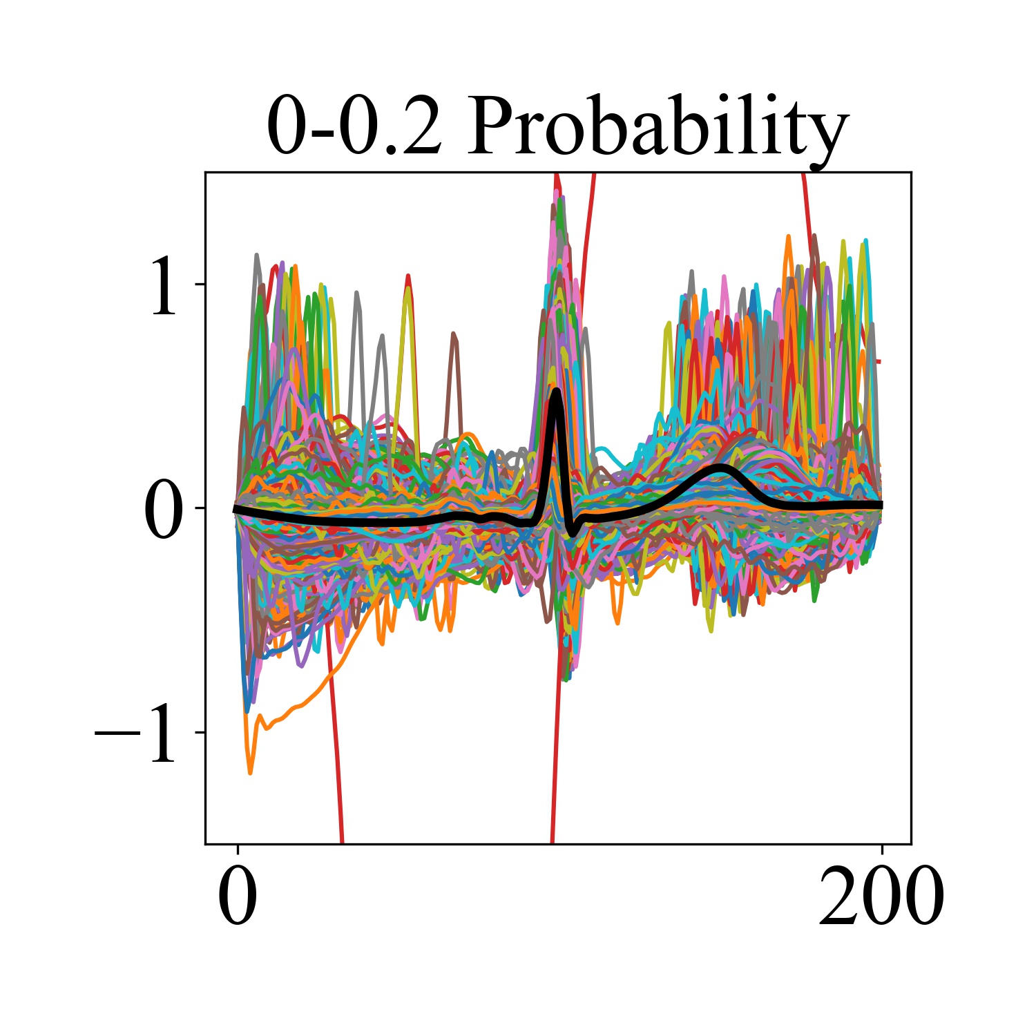
(a)

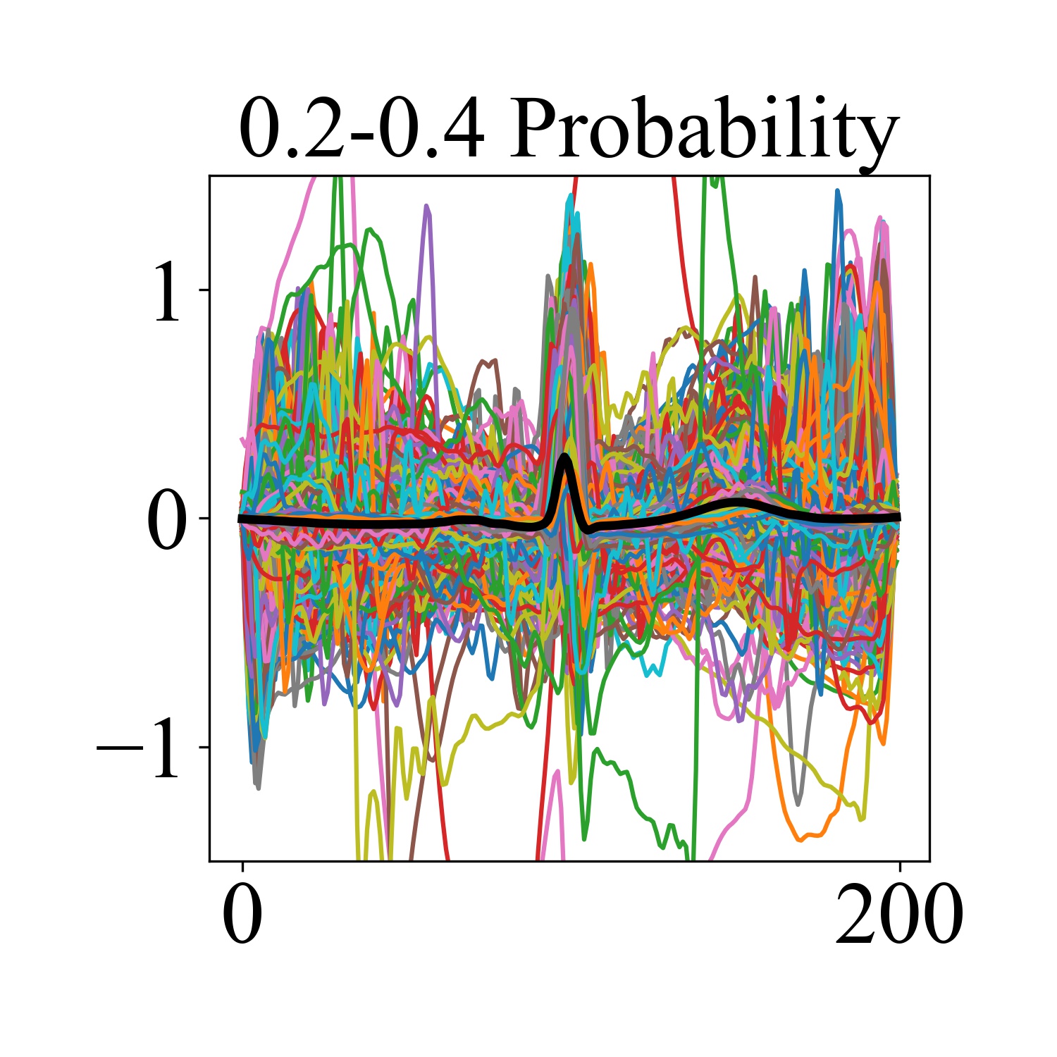
(b)

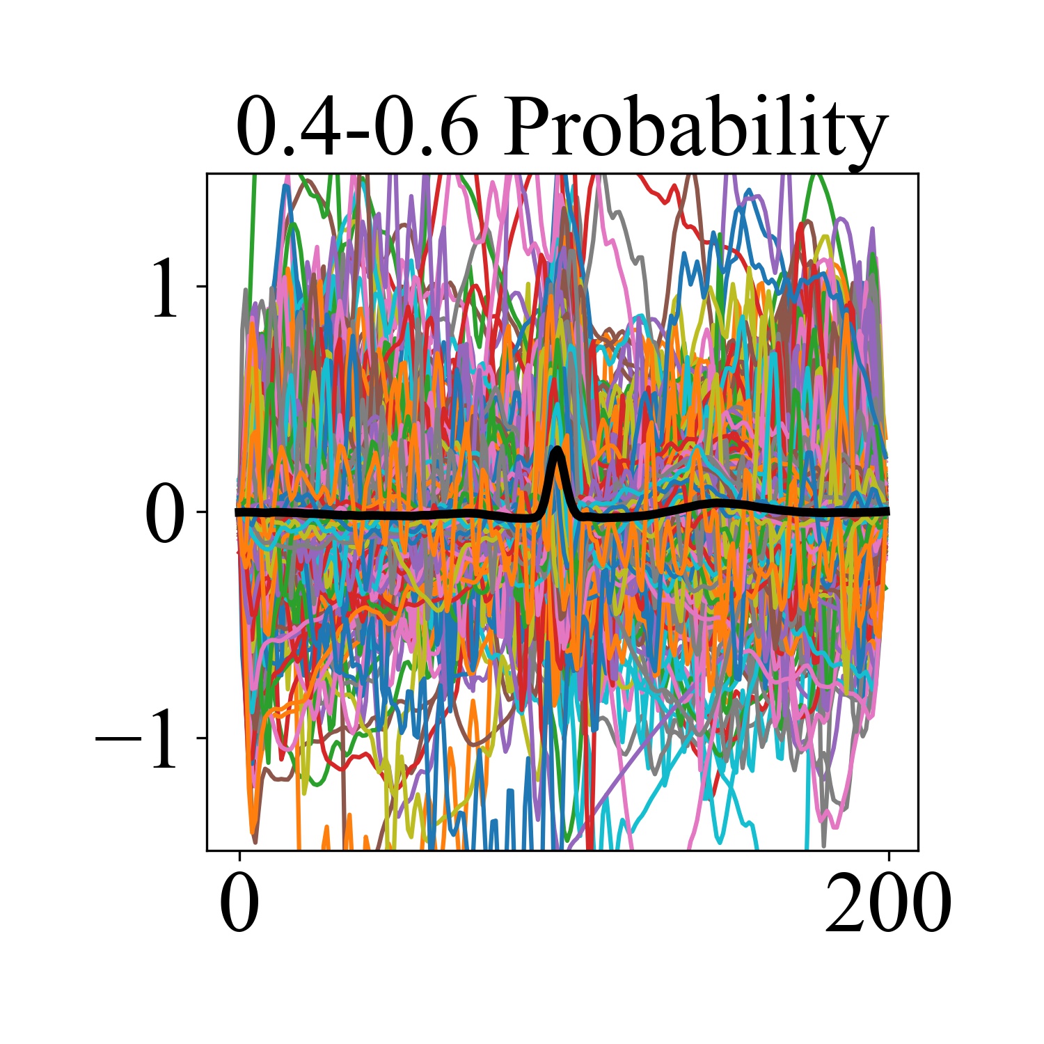
(c)

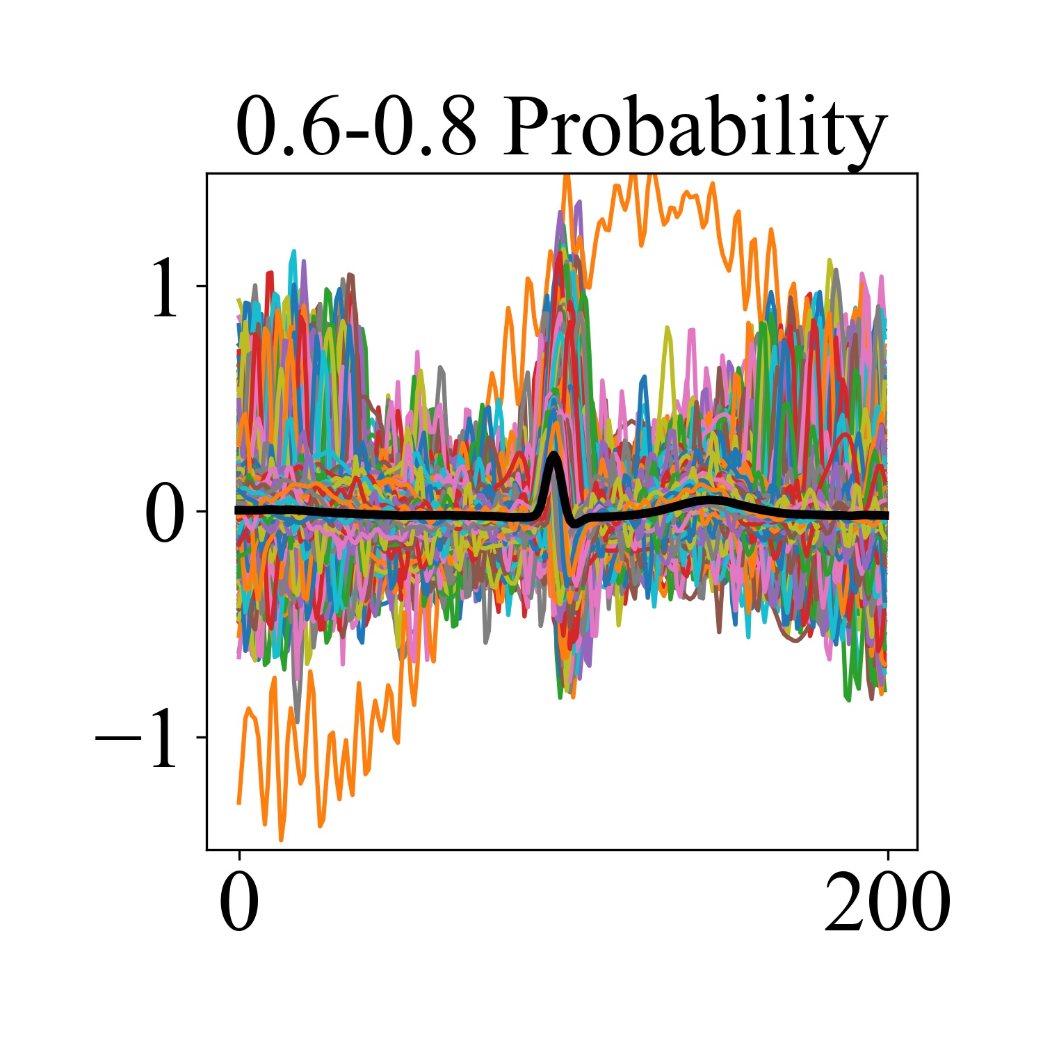
(d)

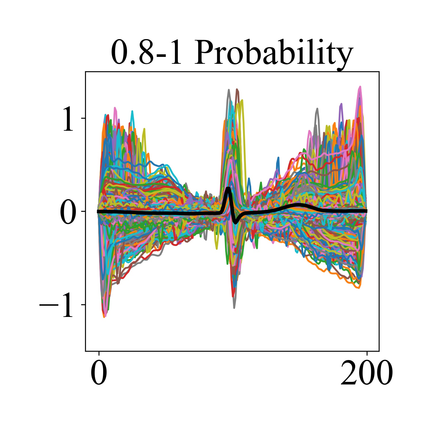
(e)

Figure 14: Average sinus beat waveforms for patients at different risk levels. After sorting the probabilities for all patients, they are equally divided into five parts, each representing a risk level. The bold black line represents the average waveform.

4.3 Subgroup analysis

We conducted subgroup analysis on beats in different states. In each model’s test results, the data were categorized into AF and non-AF, then the AF patient data were further divided into 5 categories, as detailed in Figure 3. The non-AF data remained unchanged and were combined with each of the 5 categories separately to observe the final results. The purpose of this combination was to ensure the AUC was displayed correctly.

Stable, representing a given sinus beat without the occurrence of AF in the nearby time period; Before AF, representing a given sinus beat with AF occurring in the preceding time period but not before that; After AF, representing a given sinus beat with AF occurring in the time period before it but not after that; Sinus beat near atrial premature contraction (BNA), representing a sinus beat with the occurrence of atrial premature contraction in the nearby time period; BNV, representing a sinus beat with the occurrence of premature ventricular contraction in the nearby time period. ACC, REC, PRE, F1 and AUC respectively stand for accuracy, recall, precision, and F1 score, area under curve. NoNum represents the number of beats that do not belong to this category, AbNum represents the number of beats that belong to this category, and Ratio represents the ratio of these two quantities.

Class	Index	ACC	REC	PRE	F1	AUC	# of Normal	# of AF
	1	0.5080	0.2712	0.0791	0.1225	0.3567	285317 (87.33%)	41382 (12.67%)
	2	0.4995	0.1329	0.0470	0.0694	0.2601	216377 (85.96%)	35345 (14.04%)
Stable	3	0.7134	0.4766	0.2605	0.3368	0.6674	307007 (84.73%)	55346 (15.27%)
	4	0.7319	0.3209	0.1425	0.1974	0.6367	156347 (89.73%)	17900 (10.27%)
	5	0.6426	0.2197	0.2243	0.2220	0.5395	115831 (76.80%)	34997 (23.20%)
	Avg	0.6200	0.2800	0.1500	0.1900	0.4900	216176 (85.39%)	36994 (14.61%)
	1	0.5423	0.3077	0.0000	0.0001	0.3973	285317 (100.00%)	13 (0.00%)
	2	0.5581	0.1652	0.0012	0.0024	0.3078	216377 (99.68%)	696 (0.32%)
Before AF	3	0.7545	0.1104	0.0011	0.0021	0.4415	307007 (99.76%)	734 (0.24%)
	4	0.7780	0.3786	0.0042	0.0083	0.6846	156347 (99.76%)	383 (0.24%)
	5	0.7651	0.2702	0.0123	0.0235	0.5699	115831 (98.95%)	1225 (1.05%)
	Avg	0.6800	0.2500	0.0000	0.0100	0.4800	216176 (99.72%)	610 (0.28%)
	1	0.5423	0.6667	0.0001	0.0001	0.6758	285317 (100.00%)	12 (0.00%)
	2	0.5578	0.1410	0.0013	0.0025	0.2785	216377 (99.61%)	851 (0.39%)
After AF	3	0.7548	0.2014	0.0019	0.0038	0.4933	307007 (99.77%)	720 (0.23%)
	4	0.7778	0.3013	0.0033	0.0066	0.6591	156347 (99.75%)	385 (0.25%)
	5	0.7648	0.2608	0.0124	0.0236	0.5580	115831 (98.91%)	1277 (1.09%)
	Avg	0.6800	0.3100	0.0000	0.0100	0.5300	216176 (99.70%)	649 (0.30%)
	1	0.5364	0.3965	0.0350	0.0643	0.4537	285317 (95.98%)	11942 (4.02%)
	2	0.5431	0.2014	0.0214	0.0386	0.3152	216377 (95.44%)	10339 (4.56%)
BNA	3	0.7490	0.6152	0.1182	0.1983	0.7418	307007 (94.95%)	16319 (5.05%)
	4	0.7427	0.3330	0.1176	0.1739	0.6390	156347 (91.87%)	13835 (8.13%)
	5	0.7409	0.3526	0.1044	0.1611	0.6058	115831 (92.94%)	8794 (7.06%)
	Avg	0.6600	0.3800	0.0800	0.1300	0.5500	216176 (94.64%)	12246 (5.36%)
	1	0.5460	0.7424	0.0294	0.0566	0.6960	285317 (98.17%)	5327 (1.83%)
	2	0.5647	0.7455	0.0474	0.0892	0.7249	216377 (97.14%)	6365 (2.86%)
BNV	3	0.7593	0.9108	0.0730	0.1352	0.9035	307007 (97.93%)	6478 (2.07%)
	4	0.7796	0.7993	0.1024	0.1815	0.8711	156347 (96.94%)	4932 (3.06%)
	5	0.7612	0.6246	0.1539	0.2469	0.7933	115831 (93.73%)	7744 (6.27%)
	Avg	0.6800	0.7600	0.0800	0.1400	0.8000	216176 (97.23%)	6169 (2.77%)

Table 3: The performance of beats within each classification in subgroup analysis. extbfStable, representing a given sinus beat without the occurrence of AF in the nearby time period; Before AF, representing a given sinus beat with AF occurring in the preceding time period but not before that; After AF, representing a given sinus beat with AF occurring in the time period before it but not after that; Sinus beat near atrial premature contraction (BNA), representing a sinus beat with the occurrence of atrial premature contraction in the nearby time period; BNV, representing a sinus beat with the occurrence of premature ventricular contraction in the nearby time period. # of Normal represents the number of beats that do not belong to this category, # of AF represents the number of beats that belong to this category. Time period is 10s.

The experimental results are shown in Table 3. we can observe better model performance in the BNV state, indicating a heightened likelihood of AF occurrence during ventricular arrhythmia. This discovery offers novel diagnostic insights for clinicians. However, the effectiveness of the model decreased in several other scenarios, indicating challenges in detecting AF in other situations.

4.4 Model complexity analysis

In order to illustrate the lightweight nature of the beat-level model, we compare it with the segment-level model used in [12], both predicting data during a patient’s sinus rhythm period. From Table 4, we conclude that the beat-level model is more lightweight, making it more suitable for deployment on portable medical devices compared to segment-level models.

	Beat	Segment
Total parameters	0.10M	5.90M
Training parameters	0.10M	5.89M
Computational efficiency	0.0629s	0.6784s

Table 4: Comparison of parameter quantity and computational efficiency between beat-level and segment-level models.

4.5 Interpretability and new discoveries

Beat-level Interpretability

We used CAM to visualize the interpretability of the model on beat-level data, as shown in Figure 12. CAM illustrates the model’s attention on beat prediction. Brighter colors indicate higher attention in the corresponding area, while darker colors indicate lower attention. We demonstrated situations where the model predicted high probabilities correctly and compared cases of predicting AF and non-AF. A noticeable observation is that when the data belongs to a patient with AF, the model’s correct predictions are based on the presence of a normal P-wave in the beat. In the images predicting 1 (AF), the model did not detect the P-wave, while in the images predicting 0 (non-AF), the model clearly focused on the presence of the P-wave. These findings align with the results of previous studies [33, 14, 34, 37, 10, 36], confirming the correctness and accuracy of the model’s attention to the data locations.

Beat probability trend

In the trend risk plot shown in Figure 13. The upper panel depicts ECG signals, while the lower panel illustrates the average risk probability values for temporal groups. In both cases, blue represents normal segments, and red indicates AF segments, with each group comprising 20 beats. We observed that beat prediction probabilities increase with the occurrence of AF segments. When sinus beats are around AF segments, the prediction probability is relatively high, indicating that beats around AF segments can be identified by the model. During the normal stage, where only sinus beats are detected, the prediction probability increases, suggesting that the patient is likely to experience AF in the near future.

Average waveforms

We present examples of ECG waveforms at different prediction probabilities in Figure 14. To avoid the influence of the sample size in each interval on the interval waveforms, we sort all beats by prediction probability, and then divide them into five equal parts. These plots provide a visual understanding of the model’s predictions. From Figure 14, we observe that average waveforms can to some extent reflect the health status of the patient’s beats. Due to the inherently small size of P-waves, they are not easily observed in the average waveform. However, T-waves, being relatively larger, also gradually disappear with an increase in risk probability. This indicates that when the risk probability is high, the patient’s waveform becomes highly unstable, to the extent that both P-waves and T-waves may disappear entirely.

5 Discussion

In this research, we devised a beat-level algorithm designed for identifying AF from ECG signals in sinus rhythm. While our algorithm’s AUC performance (0.7591) trails behind the segment-level algorithm AUC reported by Attia et al. (0.87-0.90) [12], such a difference was anticipated. The strength of the beat-level algorithm lies in its detailed analytical capabilities and potential for real-time monitoring, laying the groundwork for future development of more efficient information fusion decision algorithms. On the contrary, segment-level algorithms, while excelling in large-scale datasets, may encounter challenges regarding real-time applicability and portability in clinical settings.

Regarding the quantity and quality of data, it’s worth noting the distinction between the single-lead 1-second data utilized in our study and the 8-lead 10-second data employed by Attia et al. [12]. This difference holds importance in the design of algorithms for portable devices, where lightweight and fast-running algorithms are often imperative. Our algorithm showcases improved adaptability in these aspects, a crucial factor for extensive screening in environments with limited resources.

The interpretability of the model is pivotal for clinical comprehension and establishing trust in AI predictions. Our beat-level interpreter unveils the crucial role of the P-wave in AF detection, offering decision support for clinicians. In comparison, Attia et al.’s [12] segment-level model lacks this transparency, potentially constraining clinicians’ understanding of the model’s prediction results. We consider improving model interpretability as a key direction for future research.

In the experiment on the change of average risk probabilities, it was observed that sinus beats near AF segments have higher risk probabilities, providing the possibility for early warning of patients. Clinicians can focus on segments with higher risk probabilities during diagnosis and combine them with BRI for more detailed analysis.

According to the average waveforms experiment, we found that patients with higher AF risk may have more incomplete heart waveforms. Traditional research focus on the disappearance of P waves, but our research also explores the situation of T waves. The results show that in some ECGs of AF patients, T waves may be lacking or difficult to identify, which may be due to factors such as rapid heart rate and irregular rhythm.

Finally, we acknowledge limitations in only the CPSC2021 dataset, including the simplification of label assignment and the potential for overclassification, as well as the constrained number of patients. In this study, we opted for a simplified binary label assignment method, categorizing patients based solely on the presence or absence of AF episodes. This approach may introduce an overclassification issue, particularly when distinguishing between transient or infrequent AF episodes. Given that the majority of patients exhibit a dominant normal rhythm in their ECG signals, this simplified label assignment might lead to misclassifications by the model, especially in cases where AF episodes are not prominently manifested. These limitations could introduce variations in the model’s learning capacity, influencing experimental outcomes. To address these challenges, we plan to expand the dataset in future research, encompassing a more diverse range of patient populations, and refine the dataset partitioning strategy.

6 Conclusion and Future Work

In conclusion, we have established a beat-level algorithm for identifying the risk of AF in distinguishing “sinus rhythm in patients with AF” and “sinus rhythm in normal individuals”. We proposed a BRI, BID and TRI, along with several findings, showcasing meaningful clinical value. Providing timely AF risk reports to patients, enhancing collaboration between physicians and AI through the interpretability of model results, facilitates the prompt identification of AF, allowing for early intervention and treatment of this condition.

In the future, we aim to improve the model’s generalization by incorporating more high-quality datasets. Additionally, we plan to explore more rational labeling strategies based on the number or duration of AF episodes to enhance the model’s performance.

References

- [1] R. Geirhos, J.-H. Jacobsen, C. Michaelis, R. Zemel, W. Brendel, M. Bethge, F. A. Wichmann, Shortcut learning in deep neural networks, Nature Machine Intelligence 2 (11) (2020) 665–673.
- [2] A. Peimankar, S. Puthusserypady, Dens-ecg: A deep learning approach for ecg signal delineation, Expert systems with applications 165 (2021) 113911.
- [3] X. Zhang, M. Jiang, K. Polat, A. Alhudhaif, J. Hemanth, W. Wu, Detection of atrial fibrillation from variable-duration ecg signal based on time-adaptive densely network and feature enhancement strategy, IEEE Journal of Biomedical and Health Informatics 27 (2) (2022) 944–955.
- [4] X. Bao, F. Hu, Y. Xu, M. Trabelsi, E. N. Kamavuako, Paroxysmal atrial fibrillation detection by combined recurrent neural network and feature extraction on ecg signals., in: BIOSIGNALS, 2022, pp. 85–90.
- [5] Á. Huerta, A. Martinez-Rodrigo, D. Carneiro, V. Bertomeu-González, J. J. Rieta, R. Alcaraz, Comparison of supervised learning algorithms for quality assessment of wearable electrocardiograms with paroxysmal atrial fibrillation, IEEE Access (2023).
- [6] C.-P. Bernal-Oñate, E. V. Carrera, F.-M. Melgarejo-Meseguer, R. Gordillo-Orquera, A. García-Alberola, J. L. Rojo-Álvarez, Atrial fibrillation detection with spectral manifolds in low-dimensional latent spaces, IEEE Access (2023).
- [7] I. Jekova, I. Christov, V. Krasteva, Atrioventricular synchronization for detection of atrial fibrillation and flutter in one to twelve ecg leads using a dense neural network classifier, Sensors 22 (16) (2022) 6071.
- [8] C. Ma, C. Liu, X. Wang, Y. Li, S. Wei, B.-S. Lin, J. Li, A multistep paroxysmal atrial fibrillation scanning strategy in long-term ecgs, IEEE Transactions on Instrumentation and Measurement 71 (2022) 1–10.
- [9] U. R. Acharya, S. L. Oh, Y. Hagiwara, J. H. Tan, M. Adam, A. Gertych, R. San Tan, A deep convolutional neural network model to classify heartbeats, Computers in biology and medicine 89 (2017) 389–396.
- [10] D. Filos, I. Chouvarda, D. Tachmatzidis, V. Vassilikos, N. Maglaveras, Beat-to-beat p-wave morphology as a predictor of paroxysmal atrial fibrillation, Computer methods and programs in biomedicine 151 (2017) 111–121.
- [11] Y. Yue, C. Chen, P. Liu, Y. Xing, X. Zhou, Automatic detection of short-term atrial fibrillation segments based on frequency slice wavelet transform and machine learning techniques, Sensors 21 (16) (2021) 5302.
- [12] Z. I. Attia, P. A. Noseworthy, F. Lopez-Jimenez, S. J. Asirvatham, A. J. Deshmukh, B. J. Gersh, R. E. Carter, X. Yao, A. A. Rabinstein, B. J. Erickson, et al., An artificial intelligence-enabled ecg algorithm for the identification of patients with atrial fibrillation during sinus rhythm: a retrospective analysis of outcome prediction, The Lancet 394 (10201) (2019) 861–867.
- [13] A. Y. Hannun, P. Rajpurkar, M. Haghpanahi, G. H. Tison, C. Bourn, M. P. Turakhia, A. Y. Ng, Cardiologist-level arrhythmia detection and classification in ambulatory electrocardiograms using a deep neural network, Nature medicine 25 (1) (2019) 65–69.
- [14] E. Myrovali, D. Hristu-Varsakelis, D. Tachmatzidis, A. Antoniadis, V. Vassilikos, Identifying patients with paroxysmal atrial fibrillation from sinus rhythm ecg using random forests, Expert Systems with Applications 213 (2023) 118948.
- [15] F. Murat, F. Sadak, O. Yildirim, M. Talo, E. Murat, M. Karabatak, Y. Demir, R.-S. Tan, U. R. Acharya, Review of deep learning-based atrial fibrillation detection studies, International journal of environmental research and public health 18 (21) (2021) 11302.
- [16] S. Hong, C. Xiao, T. Ma, H. Li, J. Sun, Mina: Multilevel knowledge-guided attention for modeling electrocardiography signals, in: International Joint Conference on Artificial Intelligence, International Joint Conferences on Artificial Intelligence, 2019.
- [17] S. Saadatnejad, M. Oveisi, M. Hashemi, Lstm-based ecg classification for continuous monitoring on personal wearable devices, IEEE journal of biomedical and health informatics 24 (2) (2019) 515–523.
- [18] A. F. Gündüz, M. F. Talu, Atrial fibrillation classification and detection from ecg recordings, Biomedical Signal Processing and Control 82 (2023) 104531.
- [19] H. Wen, J. Kang, A comparative study on neural networks for paroxysmal atrial fibrillation events detection from electrocardiography, Journal of Electrocardiology 75 (2022) 19–27.
- [20] Y. Wang, S. Liu, H. Jia, X. Deng, C. Li, A. Wang, C. Yang, A two-step method for paroxysmal atrial fibrillation event detection based on machine learning, Mathematical Biosciences and Engineering: MBE 19 (10) (2022) 9877–9894.
-
[21]
Y. Zhou, S. Hong, J. Shang, M. Wu, Q. Wang, H. Li, J. Xie, K-margin-based residual-convolution-recurrent neural network for atrial fibrillation detection, in: Proceedings of the Twenty-Eighth International Joint Conference on Artificial Intelligence, 2019.
doi:10.24963/ijcai.2019/839.
URL http://dx.doi.org/10.24963/ijcai.2019/839 - [22] M. Gadaleta, P. Harrington, E. Barnhill, E. Hytopoulos, M. P. Turakhia, S. R. Steinhubl, G. Quer, Prediction of atrial fibrillation from at-home single-lead ecg signals without arrhythmias, NPJ Digital Medicine 6 (1) (2023) 229.
- [23] P. A. Noseworthy, Z. I. Attia, E. M. Behnken, R. E. Giblon, K. A. Bews, S. Liu, T. A. Gosse, Z. D. Linn, Y. Deng, J. Yin, et al., Artificial intelligence-guided screening for atrial fibrillation using electrocardiogram during sinus rhythm: a prospective non-randomised interventional trial, The Lancet 400 (10359) (2022) 1206–1212.
- [24] J. Torres-Soto, E. A. Ashley, Multi-task deep learning for cardiac rhythm detection in wearable devices, NPJ digital medicine 3 (1) (2020) 116.
- [25] L. Basso, Z. Ren, W. Nejdl, Efficient ecg-based atrial fibrillation detection via parameterised hypercomplex neural networks, in: 2023 31st European Signal Processing Conference (EUSIPCO), IEEE, 2023, pp. 1375–1379.
- [26] M. V. Perez, K. W. Mahaffey, H. Hedlin, J. S. Rumsfeld, A. Garcia, T. Ferris, V. Balasubramanian, A. M. Russo, A. Rajmane, L. Cheung, et al., Large-scale assessment of a smartwatch to identify atrial fibrillation, New England Journal of Medicine 381 (20) (2019) 1909–1917.
- [27] Y. Guo, H. Wang, H. Zhang, T. Liu, Z. Liang, Y. Xia, L. Yan, Y. Xing, H. Shi, S. Li, et al., Mobile health technology for atrial fibrillation screening using photoplethysmography-based smart devices: The huawei heart study, J. Am. Coll. Cardiol 74 (19) (2019) 2365–2375.
- [28] Y. An, L. Pan, L. Guo, X. Chen, Y. Shen, Percept u-net: Percept attention-based convolutional neural network for atrial fibrillation episode localization, in: 2022 IEEE 9th International Conference on Data Science and Advanced Analytics (DSAA), IEEE, 2022, pp. 1–9.
- [29] H. Jia, S. Liu, Y. Wang, D. Wang, C. Yang, A method to detect the onsets and ends of paroxysmal atrial fibrillation episodes based on sliding window and coding, in: 2022 3rd International Conference on Pattern Recognition and Machine Learning (PRML), IEEE, 2022, pp. 20–25.
- [30] M. Mehri, G. Calmon, F. Odille, J. Oster, A deep learning architecture using 3d vectorcardiogram to detect r-peaks in ecg with enhanced precision, Sensors 23 (4) (2023) 2288.
- [31] H. Wang, Z. Luo, J. W. Yip, C. Ye, M. Zhang, Ecggan: A framework for effective and interpretable electrocardiogram anomaly detection, in: Proceedings of the 29th ACM SIGKDD Conference on Knowledge Discovery and Data Mining, 2023, pp. 5071–5081.
- [32] S. Hong, Y. Xu, A. Khare, S. Priambada, K. Maher, A. Aljiffry, J. Sun, A. Tumanov, Holmes: Health online model ensemble serving for deep learning models in intensive care units, in: Proceedings of the 26th ACM SIGKDD International Conference on Knowledge Discovery & Data Mining, 2020, pp. 1614–1624.
- [33] G. Giannopoulos, D. Tachmatzidis, D. V. Moysidis, D. Filos, M. Petridou, I. Chouvarda, V. P. Vassilikos, P-wave indices as predictors of atrial fibrillation: the lion from a claw, Current Problems in Cardiology (2023) 102051.
- [34] A. Martínez, R. Alcaraz, J. J. Rieta, Morphological variability of the p-wave for premature envision of paroxysmal atrial fibrillation events, Physiological measurement 35 (1) (2013) 1.
- [35] S. Khurshid, S. Friedman, C. Reeder, P. Di Achille, N. Diamant, P. Singh, L. X. Harrington, X. Wang, M. A. Al-Alusi, G. Sarma, et al., Ecg-based deep learning and clinical risk factors to predict atrial fibrillation, Circulation 145 (2) (2022) 122–133.
- [36] D. Tachmatzidis, D. Filos, I. Chouvarda, A. Tsarouchas, D. Mouselimis, C. Bakogiannis, C. Lazaridis, K. Triantafyllou, A. P. Antoniadis, N. Fragakis, et al., Beat-to-beat p-wave analysis outperforms conventional p-wave indices in identifying patients with a history of paroxysmal atrial fibrillation during sinus rhythm, Diagnostics 11 (9) (2021) 1694.
- [37] G. Conte, A. Luca, S. Yazdani, M. L. Caputo, F. Regoli, T. Moccetti, L. Kappenberger, J.-M. Vesin, A. Auricchio, Usefulness of p-wave duration and morphologic variability to identify patients prone to paroxysmal atrial fibrillation, The American journal of cardiology 119 (2) (2017) 275–279.
- [38] X. Wang, C. Ma, X. Zhang, H. Gao, G. D. Clifford, C. Liu, Paroxysmal atrial fibrillation events detection from dynamic ecg recordings: The 4th china physiological signal challenge 2021, Proc. PhysioNet (2021) 1–83.
- [39] F. Bozyigit, F. Erdemir, M. Sahin, D. Kilinc, Classification of electrocardiogram (ecg) data using deep learning methods, in: 2020 4th International Symposium on Multidisciplinary Studies and Innovative Technologies (ISMSIT), IEEE, 2020, pp. 1–5.