Spatially Randomized Designs Can Enhance Policy Evaluation

Abstract

This article studies the benefits of using spatially randomized experimental designs which partition the experimental area into distinct, non-overlapping units with treatments assigned randomly. Such designs offer improved policy evaluation in online experiments by providing more precise policy value estimators and more effective A/B testing algorithms than traditional global designs, which apply the same treatment across all units simultaneously. We examine both parametric and nonparametric methods for estimating and inferring policy values based on this randomized approach. Our analysis includes evaluating the mean squared error of the treatment effect estimator and the statistical power of the associated tests. Additionally, we extend our findings to experiments with spatio-temporal dependencies, where treatments are allocated sequentially over time, and account for potential temporal carryover effects. Our theoretical insights are supported by comprehensive numerical experiments.

Keywords: A/B testing, policy evaluation, reinforcement learning, spatially randomized designs.

1 Introduction

Policy evaluation in spatially dependent experiments involves analyzing spatially referenced data to assess the impact of new products. This methodology is widely used in diverse fields, including environmental studies (Zigler et al. 2012), epidemiology (Hudgens and Halloran 2008), social science (Sobel 2006), and technology industries (Zhou et al. 2020). In such experiments, the challenge often lies in the limited number of observations and the small magnitude of treatment effects. Moreover, the strong interconnections among spatial units tend to increase the variance of estimations, making the detection of subtle effects difficult. Additionally, the treatment effect on one spatial unit may extend to neighboring units, leading to a breach of the stable unit treatment value assumption (SUTVA, see, e.g., Imbens and Rubin 2015), and causing interference or spillover effects that complicate the analysis.

To exemplify, let’s look at ride-sourcing platforms like Uber, Lyft, and Didi Chuxing, which serve as two-sided marketplaces linking passengers with drivers (Rysman 2009). These companies extensively utilize A/B testing to assess the efficacy of universal treatment policies, such as new order dispatch or subsidy strategies implemented across an entire city (Xu et al. 2018, Zhou et al. 2021, Shi et al. 2022, Luo et al. 2024). In these settings, the dynamic networks of call orders and available drivers represent the supply and demand within these marketplaces, exhibiting significant spatial correlations (Ke et al. 2018). Moreover, budget limitations often restrict the duration of online experiments to a mere two weeks (Shi et al. 2023), with the anticipated improvements from novel policies being relatively modest, typically between 0.5% and 2% (Tang et al. 2019). To understand the spillover effects, consider that implementing a subsidy policy for drivers in one area might draw drivers from adjacent regions, thereby influencing outcomes in those neighboring areas as well. This interconnection underscores the need for innovative experimental design theories and policy evaluation methodologies to accurately infer causal effects in such complex online environments.

This study aims to rigorously assess the effectiveness of various experimental designs in spatially and spatio-temporally dependent experiments. In the realm of clinical trials, numerous adaptive designs have been developed, allowing treatments to be tailored to participants based on specific criteria and personal information (see e.g., Taves 1974, Pocock and Simon 1975, Kalish and Begg 1985, Rosenberger and Sverdlov 2008, Hu and Hu 2012). These designs have proven to enhance the precision of average treatment effect estimators in traditional settings where observations are independent and identically distributed (i.i.d.), devoid of spatial or temporal interdependencies. Yet, the application and efficacy of these designs in experiments with spatial dependencies remain largely unexplored.

Our contributions are multifolds, summarized as follows: Firstly, we systematically study the theoretical properties of three major spatial designs: (i) An on-policy global design that uniformly applies the same treatment across all spatial units for each time period. (ii) An individual-randomized design where spatial units are randomized on an individual basis into treatment or control groups, ensuring independent treatment assignments among different spatial units. (iii) A cluster-randomized design that groups adjacent spatial units into clusters based on their spatial locations, with these clusters then independently randomized into treatment or control groups. Secondly, we have employed advanced parametric and semiparametric methodologies for estimating and inferring the treatment effects derived from these spatial designs. Our analysis extends to examining the mean squared errors (MSE) of these estimators and the effectiveness (power) of the corresponding hypothesis tests. Thirdly, our investigations uncover a notable insight: under conditions of spatial correlation and precise modeling of spatial spillover/interference effects, the off-policy estimators, derived from spatially randomized designs, can surpass the efficiency of on-policy estimators from a global policy framework. Fourthly, we broaden our theoretical insights to encompass experiments influenced by spatio-temporal dependencies, enhancing the applicability of our findings to more complex and dynamic settings. This comprehensive analysis not only advances the understanding of spatial experimental designs but also highlights the potential for increased efficiency in policy evaluation through nuanced modeling of spatial dynamics.

1.1 Related work

Experimental designs with interference. Previous literature has predominantly concentrated on the i.i.d. setting, yet there’s a burgeoning interest in experimental designs that accommodate spatial or network interference (Ugander et al. 2013, Baird et al. 2018, Basse and Airoldi 2018, Jagadeesan et al. 2020, Li et al. 2019, Viviano 2020, Zhou et al. 2020, Kong et al. 2021, Leung 2022). These works commonly address where each experimental unit only receives one treatment. As a result, the global design, which would require each unit to be exposed to both treatment and control policies, is not applicable to this scenario. The trade-off between the global design and spatially randomized designs is not explored in these papers. On the contrary, we focus on a different setup with repeated measurements in which each unit receives a sequence of treatments over time. Our context includes applications that entail sequential decision making over time. Our approach not only broadens the applicability of experimental designs but also introduces novel considerations for managing spatial and temporal dependencies.

More recently, there have been a few newly developed experimental designs that are motivated by the applications in technological companies with other type of interference, including the multiple randomization design in two-sided platforms (Bajari et al. 2021, Johari et al. 2022, Xiong et al. 2023) and the equilibrium design (Wager and Xu 2021). However, these papers differ from ours in terms of the experimental settings considered. For example, Bajari et al. (2021) and Johari et al. (2022) studied settings in which interventions are assigned to two or multiple populations interacting with each other (e.g., buyer-seller pairs). On the other hand, spatial dependent experiments considered in this work involve multiple spatial units receiving different treatments at each time.

Spatial causal inference with interference. Research on spatial interference has primarily branched into two prominent types of methods. The first type is built on the concept of partial interference, segmenting individuals into clusters with the interference effects contained within each respective cluster (Halloran and Struchiner 1991, 1995, Liu et al. 2016, Zigler and Papadogeorgou 2021). The second type adopts the principle of local or network interference, wherein the interference effects are confined to the immediate vicinity or network surrounding each node, a perspective supported by the works of Verbitsky-Savitz and Raudenbush (2012), Perez-Heydrich et al. (2014), Puelz et al. (2022). Recent studies have ventured beyond these traditional frameworks, proposing more flexible interference models that accommodate a broader range of interactions (Aronow and Samii 2017, Tchetgen et al. 2021). Furthermore, some researchers have explored alternative conceptual models, such as diffusion processes and market equilibrium, to simplify the complexity inherent in these systems (Larsen et al. 2022, Munro et al. 2021). Despite the extensive exploration of interference effects and their mechanisms, a notable gap in the literature is the specific consideration of experimental designs tailored to these contexts. We aim to bridge this gap by focusing on the development and analysis of experimental designs optimized for spatially dependent settings.

Off-policy evaluation (OPE). Our research intersects with an expanding domain of scholarship on OPE within the realm of sequential decision-making processes (see e.g, Uehara et al. 2022, for a review). OPE is concerned with assessing the effectiveness of a target policy without active deployment, instead utilizing pre-existing data collected under a different, behavior-guiding policy. In the context of finite-horizon settings characterized by a limited number of decision points, augmented inverse propensity score weighted estimators have been introduced (Zhang et al. 2013, Jiang and Li 2016, Luedtke and Van Der Laan 2016, Thomas and Brunskill 2016). More recent advancements have extended these methodologies to efficiently handle evaluations over extended or infinite time horizons (Liao et al. 2021, Shi et al. 2021, Wang et al. 2023, Liao et al. 2022, Kallus and Uehara 2022). These studies have not explored policy evaluation in the context of spatial dependence or the role of experimental design in such settings.

2 Nondynamic Setting

We start our exploration in a nondynamic setting, also known as the contextual bandit scenario. In this environment, prior interventions do not influence subsequent outcomes, thus excluding any potential temporal spillover effects. The examination of a dynamic setting, where such carryover impacts are considered, will be undertaken in the subsequent section.

2.1 Problem formulation

Consider a city divided into $R$ non-overlapping spatial units, with an interest in assessing the efficacy of a novel city-level policy compared to a conventional control. For the $\iota$th region, let $Y_{\iota}(1)$ and $Y_{\iota}(0)$ represent the potential daily outcomes under the new and existing policies, respectively. Our primary focus is on determining the overall average treatment effect (ATE), expressed as:

$${\tau}=\sum_{\iota=1}^{R}{\mathbb{E}}\left\{Y_{\iota}(1)-Y_{\iota}(0)\right\}.$$

To estimate the ATE, we conduct an online experiment, concentrating on experimental designs that ensure uniform policy application across all city units for each day. Moreover, we assume that data collected on different days are independent, eliminating the influence of previous policy implementations on subsequent outcomes.

The primary aim of this study is to evaluate the performance of spatially randomized designs in comparison to a global design, aiming to shed lights on their effects on the mean square error (MSE) of the resulting ATE estimator and the power of A/B testing procedures. In the global design framework, a uniform policy is applied across all $R$ units for each day, which can be mathematically represented as: $A_{1}=A_{2}=\cdots=A_{R},$ with certainty, for any given day $t$. Here, $A_{\iota}$ signifies the binary treatment indicator for the $\iota$th region on day $t$. In contrast, spatially randomized designs spatially randomized designs allow these $A_{\iota}$s to be different at each time. This paper studies two specific types of spatially randomized designs: an individual-randomized design and a cluster-randomized design. The individual-randomized design allocates treatments to each $A_{\iota}$ independently, ensuring that each has a non-zero probability $p_{\iota}$ of receiving treatment 1 (and a corresponding $1-p_{\iota}$ probability of not receiving it). Conversely, the cluster-randomized design organizes units into $m$ distinct, non-overlapping clusters based on their spatial proximity, ensuring uniform treatment within each cluster. In other words, let $\mathcal{C}_{j}$ denote the indices of regions that belong to the $j$th cluster, we have $A_{k_{1}}=A_{k_{2}}=A^{(j)}$ for any $k_{1},k_{2}\in\mathcal{C}_{j}$. The treatment for each cluster is determined independently, with $p^{(j)}$ representing the likelihood of the $j$th cluster receiving treatment 1. It is noteworthy that the individual-randomized design can essentially be regarded as a specific form of the cluster-randomized design, where each cluster corresponds to an individual unit, i.e., $m=R$ and $\mathcal{C}_{j}=j$ for every $j$.

Furthermore, we are interested in testing the following pair of hypotheses as well

$$H_{0}:{\tau}\leq 0\text{\ \ V.S.\ \ }H_{1}:{\tau}>0.$$ (1)

Under the null hypothesis, the relative improvement of benefits brought by the new policy is relatively low in comparison to the associated implementation costs. As such, we recommend to use the standard control.

2.2 A toy example

Before comparing these designs in general scenarios, we start with a simple yet illustrative example to highlight the advantages of spatially randomized designs over the global approach. Consider a city partitioned into two distinct regions, leading to a total of $R=2$ regions, with the experiment spanning $N$ days. The collected data is represented as $\{(A_{t,\iota},Y_{t,\iota}):\iota=1,2;1\leq t\leq N\}$, where $t$ denotes the day, and $Y_{t,\iota}$ is the outcome for region $\iota$ on day $t$. The underlying model for the outcomes is given by:

$$Y_{t,\iota}=\alpha_{j}+\gamma_{j}A_{t,\iota}+e_{t,\iota},$$ (2)

where the error terms $\{e_{t,\iota}:1\leq t\leq N\}$ are assumed to be i.i.d with zero mean (${\mathbb{E}}e_{t,1}={\mathbb{E}}e_{t,2}=0$) and constant variance (${\mbox{Var}}(e_{t,1})={\mbox{Var}}(e_{t,2})=\sigma^{2}$). The correlation between the errors in the two regions on the same day is denoted by $\rho$. In an idealized scenario, these errors might be considered independent with $\rho=0$. However, as previously discussed, spatial correlation typically results in $\rho\neq 0$ due to shared environmental factors, such as holidays, extreme weather events, or significant disruptions in services like ride-sourcing, that have a simultaneous impact on both regions, suggesting a positive correlation ($\rho>0$).

Under model (2), ATE equals ${\tau}=\gamma_{1}+\gamma_{2}$. We examine two distinct experimental frameworks. The first employs a global design, where $A_{t,1}$ and $A_{t,2}$ are uniformly set to $A_{t}^{g}$, which are i.i.d. Bernoulli(0.5) random variables. Alternatively, we explore a unique spatially randomized design, characterized by independently setting both $\mathbb{P}(A_{t,1}=1)$ and $\mathbb{P}(A_{t,2}=1)$ to 0.5. Notably, under this spatial design, there is approximately a 50% likelihood that the treatments allocated to the two regions will be different at any given time. As we will demonstrate, this strategic allocation significantly diminishes the MSE of the ATE estimator, particularly in scenarios where the errors $e_{t,1}$ and $e_{t,2}$ exhibit a positive correlation.

Let $Y_{t}=\sum_{\iota=1}^{2}Y_{t,\iota}$. The ATE estimators under the two designs are given by

$$\widehat{{\tau}}^{g} = \frac{\sum_{t=1}^{N}Y_{t}A_{t}^{g}}{\sum_{t=1}^{N}A_{t}^{g}}-\frac{\sum_{t=1}^{N}Y_{t}\left(1-A_{t}^{g}\right)}{\sum_{t=1}^{N}\left(1-A_{t}^{g}\right)},$$

$$\widehat{{\tau}}^{s} = \frac{\sum_{t=1}^{N}Y_{t,1}A_{t,1}}{\sum_{t=1}^{N}A_{t,1}}-\frac{\sum_{t=1}^{N}Y_{t,1}\left(1-A_{t,1}\right)}{\sum_{t=1}^{N}\left(1-A_{t,1}\right)}+\frac{\sum_{t=1}^{N}Y_{t,2}A_{t,2}}{\sum_{t=1}^{N}A_{t,2}}-\frac{\sum_{t=1}^{N}Y_{t,2}\left(1-A_{t,2}\right)}{\sum_{t=1}^{N}\left(1-A_{t,2}\right)}.$$

We follow the causal inference literature and assume the consistency assumption (CA) and SUTVA as follows:
$-$CA. For any $t$ and $\iota$, $Y_{t,\iota}$ equals to the potential outcome $Y_{t,\iota}(A_{t,\iota})$.
$-$SUVTA. For any $\iota$, the $\iota$th region’s outcome is independent of any other region’s treatment. Then both $\widehat{{\tau}}^{g}$ and $\widehat{{\tau}}^{s}$ are unbiased esimators. In addition, with some calculations, one can show that

$${\mbox{Var}}\left(\widehat{{\tau}}^{g}\right)=\frac{4}{N}{\mbox{Var}}\left(e_{t,1}+e_{t,2}\right)=\frac{8(1+\rho)\sigma^{2}}{N}\quad\mbox{and}~{}~{}{\mbox{Var}}\left(\widehat{{\tau}}^{s}\right)=\frac{4}{N}[{\mbox{Var}}(e_{t,1})+{\mbox{Var}}(e_{i2})]=\frac{8\sigma^{2}}{N}.$$

As such, ${\operatorname{MSE}}\left(\widehat{{\tau}}^{g}\right)>{\operatorname{MSE}}\left(\widehat{{\tau}}^{s}\right)$ whenever $\rho>0$. In particular, when $\rho=0.5$, the MSE under the global design is 1.5 times larger than that under the spatially randomized design.

To understand why spatially randomized designs can enhance policy evaluation, notice that under this design, $A_{t,1}$ and $A_{t,2}$ might receive opposite values. When this occurs, the difference between outcomes $Y_{t,1}$ and $Y_{t,2}$ is used to construct the ATE estimator. When the errors $e_{t,1}$ and $e_{t,2}$ exhibit positive correlation, by contrasting $Y_{t,1}$ and $Y_{t,2}$, we effectively reduce the variance of the ATE estimator.

It is important to note, however, that this analysis is based on the assumption of no spillover effects between units (or SUTVA). In the subsequent analysis, we will consider these spillover effects and demonstrate the advantages of spatially randomized designs, assuming these effects can be precisely estimated. Additionally, the conditions of unconfoundedness and positivity, which are crucial in causal inference and the study of personalized treatment regimes (see e.g., Robins et al. 2000, Zhang et al. 2012, 2015, Wang et al. 2018, Shi et al. 2021), are naturally met in both the global and spatial designs discussed.

2.3 Data, parametric and semiparametric learning

Data. In the general, nondynamic framework, we consider $R$ distinct, non-intersecting regions. Our analysis includes treatment-outcome pairs $\{(A_{t,\iota},Y_{t,\iota}):1\leq t\leq N,1\leq\iota\leq R\}$ along with a set of pre-treatment observational variables $\{O_{t,\iota}\}_{t,\iota}$, which measures important characteristics of the environment, like the initial number of drivers in a ride-sharing market. These variables are introduced to further enhance the precision of the ATE estimator. The MSE of the ATE estimator and the efficacy of the corresponding tests are influenced by the chosen estimation and inference procedures. In this study, we explore two approaches: one leveraging parametric models and the other employing semiparametric methods.

Parametric learning. We introduce a parametric outcome model, positing that the outcome for a given region is a composite function of its observations, treatment, and the treatments of adjacent regions:

$$Y_{t,\iota}=\alpha_{\iota}+O_{t,\iota}^{\top}\beta_{\iota}+\gamma_{\iota}A_{t,\iota}+f_{\theta_{\iota}}\left(\{A_{t,j}\}_{j\in\mathcal{N}_{\iota}}\right)+e_{t,\iota},$$ (3)

where $\alpha_{\iota},\gamma_{\iota}\in\mathbb{R}$, $\beta_{\iota}\in\mathbb{R}^{d}$, and $\mathcal{N}_{\iota}$ represents the neighboring regions of the $\iota$th region. The errors $\{e_{t,\iota}\}$ are assumed to be zero-mean, temporally independent, and spatially correlated, and independent from observations and treatments. The function $f_{\theta_{\iota}}(\cdot)$ captures spatial spillover effects. This model allows a region’s outcome to depend on the treatments of its neighbors while maintaining conditional independence from treatments in non-neighboring regions, a common assumption in spatial analysis literature (see e.g., Reich et al. 2021). This is particularly relevant in contexts like ride-sharing markets, where a policy’s impact in one area can affect neighboring areas through driver distribution, assuming drivers can only move to adjacent areas within a given time frame. The form of $f_{\theta_{\iota}}(\cdot)$ can vary, with examples including $\sum_{j\in\mathcal{N}_{\iota}}\theta_{\iota j}A_{t,j}$ and $\theta_{\iota}\overline{A}_{t,\mathcal{N}_{\iota}}$, where $\overline{A}_{t,\mathcal{N}\iota}=n_{\iota}^{-1}\sum_{k\in\mathcal{N}\iota}A_{ik}$ and $n_{\iota}=|\mathcal{N}_{\iota}|$. Our focus is on the latter formulation, though our findings can be extended to other functional forms as discussed in related literature.

Under the global design and the linearity assumption that $f_{\theta_{\iota}}(\{A_{t,j}\}_{j\in\mathcal{N}_{\iota}})=\theta_{\iota}\overline{A}_{t,\mathcal{N}_{\iota}}$, different spatial units receive the same treatment and their outcomes satisfy

$$Y_{t,\iota}=\alpha_{\iota}+O_{t,\iota}^{\top}\beta_{\iota}+\gamma_{\iota}^{g}A_{t}+e_{i\iota},$$ (4)

where $\gamma_{\iota}^{g}=\gamma_{\iota}+\theta_{\iota}$. It is immediate to see that ATE has the following closed-form expression,

$${\tau}=\sum_{\iota=1}^{R}\gamma_{\iota}^{g}=\sum_{\iota=1}^{R}\left(\gamma_{\iota}+\theta_{\iota}\right).$$

Using data collected from the global design, we apply the ordinary least square (OLS) regression to estimate $\gamma_{\iota}^{g}$ based on (4) and plug-in these estimators to estimate the ATE, leading to

$$\widehat{\tau}^{g}=\sum_{\iota=1}^{R}\widehat{\gamma}_{\iota}^{g}=\sum_{\iota=1}^{R}u_{3}^{\top}\left\{\sum_{t=1}^{N}Z_{t,\iota}^{g}\left(Z_{t,\iota}^{g}\right)^{\top}\right\}^{-1}\left(\sum_{t=1}^{N}Z_{t,\iota}^{g}Y_{t,\iota}\right),$$ (5)

where $u_{3}=(0,0,1)^{\top}$ and $Z_{t,\iota}^{g}=(1,O_{t,\iota}^{\top},A_{t})^{\top}$.

In the individual-randomized design, we adjust $\gamma_{\iota}^{g}$ by splitting it into $\gamma_{\iota}+\theta_{\iota}$ and apply OLS to estimate these parameters from the model. The estimators obtained are denoted as $\widehat{\gamma}_{\iota}^{i}$ and $\widehat{\theta}_{\iota}^{i}$. For the cluster-randomized design, we define $\mathcal{C}_{j}^{0}$ as the set of interior regions and $\partial\mathcal{C}_{j}$ as the boundary regions of $\mathcal{C}_{j}$. A region in $\mathcal{C}_{j}^{0}$ is surrounded by neighbors all within the same cluster $\mathcal{C}_{j}$. In contrast, a boundary region in $\partial\mathcal{C}_{j}$ has at least one neighbor outside of $\mathcal{C}_{j}$. For these boundary regions, we estimate the regression coefficients $\widehat{\gamma}_{\iota}^{c}$ and $\widehat{\theta}_{\iota}^{c}$ using OLS, similar to the individual-randomized approach. However, in the interior regions, where treatments are consistent across neighboring areas, $\gamma_{\iota}$ and $\theta_{\iota}$ cannot be distinguished, leading us to estimate their combined effect using OLS, similar to the global design. This procedure yields the following plug-in estimators for ${\tau}$:

$$\widehat{\tau}^{i}=\sum_{\iota=1}^{R}u_{34}^{\top}\left\{\sum_{t=1}^{N}Z_{t,\iota}^{i}\left(Z_{t,\iota}^{i}\right)^{\top}\right\}^{-1}\left(\sum_{t=1}^{N}Z_{t,\iota}^{i}Y_{t,\iota}\right),\ \ \widehat{\tau}^{c}=\sum_{j=1}^{m}\sum_{\iota\in\mathcal{C}_{j}}^{R}u_{\iota}^{\top}\left\{\sum_{t=1}^{N}Z_{t,\iota}^{c}\left(Z_{t,\iota}^{c}\right)^{\top}\right\}^{-1}\left(\sum_{t=1}^{N}Z_{t,\iota}^{c}Y_{t,\iota}\right),$$ (6)

where $u_{34}=(0,0,1,1)^{\top}$, $Z_{t,\iota}^{i}=(1,O_{t,\iota}^{\top},A_{t,\iota},\overline{A}_{t,\mathcal{N}_{\iota}})^{\top}$, $u_{\iota}^{c}=u_{34}\mathbb{I}\{\iota\in\partial\mathcal{C}_{j}\}+u_{3}\mathbb{I}\{\iota\in\mathcal{C}_{j}^{0}\}$, and $Z_{t,\iota}^{c}=(1,O_{t,\iota}^{\top},A_{t}^{(j)},\overline{A}_{t,\mathcal{N}_{\iota}})^{\top}\mathbb{I}\{\iota\in\partial\mathcal{C}_{j}\}+(1,O_{t,\iota}^{\top},A_{t}^{(j)})^{\top}\mathbb{I}\{\iota\in\mathcal{C}_{j}^{0}\}$.

Semiparametric learning. We now explore the concept of doubly robust estimators for ATE, which are highly regarded in the field of semiparametric statistics due to their effectiveness and resilience against model inaccuracies (see e.g., Tsiatis 2006, Chernozhukov et al. 2018). These estimators are termed “doubly robust” because their accuracy depends on the correct specification of either the outcome regression model or the propensity score model, but not necessarily both.

For the outcome regression, we propose the following model for the observed outcomes $Y_{t,\iota}$:

$$Y_{t,\iota}=h_{\iota}(A_{t,\iota},\overline{A}_{t,\iota},O_{t,\iota},\overline{O}_{t,\iota})+e_{t,\iota},$$ (7)

where the error terms $\{e_{t,\iota}\}_{t,\iota}$s are temporally independent, spatially correlated, and independent of the observed covariates $\{O_{t,\iota}\}$s and treatments $\{A_{t,\iota}\}$s. This model acknowledges spatial interdependencies by allowing a region’s outcome to be influenced by its own treatment as well as the average treatment among its neighbors, thereby extending the traditional SUTVA to accommodate spatial interactions.

Model (7) enhances our analytical framework in two significant ways: firstly, it does not constrain the form of $h_{\iota}$, thereby permitting the use of nonparametric regression or machine learning techniques for estimation; secondly, it incorporates the influence of neighboring covariates $\overline{O}_{t,\iota}$, calculated as the average of $O_{t,\iota}$ across neighboring regions. This addition enriches the model by allowing more broader spatial contexts in the outcome regression model. Assuming consistency, where the potential outcome for each region depends solely on the set of treatments applied across all regions, the ATE can be expressed as

$${\tau}=\sum_{\iota=1}^{R}{\mathbb{E}}[h_{\iota}(1,1,O_{t,\iota},\overline{O}_{t,\iota})-h_{\iota}(0,0,O_{t,\iota},\overline{O}_{t,\iota})].$$

To motivate the doubly robust estimator, we define the following estimating function for any $1\leq\iota\leq R$, $1\leq t\leq N$ and $a\in\{0,1\}$,

$${\nu}_{DR}(a,\iota,t,h_{\iota},\pi_{\iota})=\frac{\mathbb{I}(A_{t,\iota}=a,\overline{A}_{t,\iota}=a)}{{\pi}_{\iota}(a|\{O_{t,j}\}_{j})}[Y_{t,\iota}-{h}_{\iota}(a,a,O_{t,\iota},\overline{O}_{t,\iota})]+{h}_{\iota}(a,a,O_{t,\iota},\overline{O}_{t,\iota}),$$ (8)

where $\mathbb{I}(\bullet)$ denotes the indicator function and ${\pi}_{\iota}(a|\{O_{t,j}\}_{j})$ denotes the propensity score $\mathbb{P}(A_{t,\iota}=a,\overline{A}_{t,\iota}=a|\{O_{t,j}\}_{j})$. It can be shown by straightforward calculations that ${\nu}_{DR}(a,\iota,t,h_{\iota},\pi_{\iota})$ is an unbiased estimator for ${\mathbb{E}}Y_{t,\iota}(\{a\})$, provided that at least one of $\pi_{\iota}$ or $h_{\iota}$ is accurately specified. This leads to the following estimator for the treatment effect $\tau$:

$$\frac{1}{N}\sum_{\iota=1}^{R}\sum_{t=1}^{N}[{\nu}_{DR}(1,\iota,t,\widehat{h}_{\iota},\widehat{\pi}_{\iota})-{\nu}_{DR}(0,\iota,t,\widehat{h}_{\iota},\widehat{\pi}_{\iota})],$$

where $\widehat{h}_{\iota}$ and $\widehat{\pi}_{\iota}$ are estimators of $h_{\iota}$ and $\pi_{\iota}$, respectively, obtained via suitable supervised learning techniques.

Within the framework of spatially randomized designs, $\pi_{\iota}$ is predetermined and remains unaffected by observational data. Specifically, under the individual-randomized and cluster-randomized designs, the propensity scores are denoted by $\pi_{\iota}^{i}$ and $\pi_{\iota}^{c}$, respectively. For the individual-randomized design, the propensity score for any region $\iota$ and its neighbors can be expressed as:

$$\pi_{\iota}^{i}(a)=p_{\iota}^{a}(1-p_{\iota})^{1-a}\prod_{j\in\mathcal{N}_{\iota}}[p_{j}^{a}(1-p_{j})^{1-a}].$$

In the context of the cluster-randomized design, for regions $\iota$ located entirely within a cluster $\mathcal{C}_{j}^{0}$, the propensity score simplifies to $\pi_{\iota}^{c}(a)=(p^{(j)})^{a}(1-p^{(j)})^{1-a}$. Conversely, for regions $\iota$ on the boundary of a cluster $\partial\mathcal{C}_{j}$, the propensity score is given by:

$$\pi_{\iota}^{c}(a)=(p^{(j)})^{a}(1-p^{(j)})^{1-a}\prod_{k\neq j}\Big{[}\Big{\{}1-\prod_{i\in\mathcal{N}_{\iota}}\mathbb{I}(i\notin\mathcal{C}_{k})\Big{\}}(p^{(k)})^{a}(1-p^{(k)})^{1-a}+\prod_{i\in\mathcal{N}_{\iota}}\mathbb{I}(i\notin\mathcal{C}_{k})\Big{]}.$$

This formulation accounts for the complex interplay between the treatment assignments of neighboring regions and the spatial structure of the clusters.

To circumvent the need for imposing stringent metric entropy conditions on the outcome regression function (Díaz 2020), we adopt a strategy that involves data-splitting and cross-fitting (Chernozhukov et al. 2018). This approach involves partitioning the dataset into several segments, using one segment to estimate the outcome regression function $h_{\iota}$, and utilizing the remainder of the data for ATE estimation. This process is repeated across different data partitions, ensuring that each segment is used exactly once for $h_{\iota}$ estimation and once for ATE estimation. The final ATE estimators are then derived by aggregating the estimations from all partitions, thereby achieving maximal statistical efficiency. The detailed steps of this methodology are delineated in Algorithm 1.

Algorithm 1 Doubly robust estimation in nondynamic settings

Data $\{(O_{t,\iota},A_{t,\iota},Y_{t,\iota})\}_{t,\iota}$ collected from a given design.

1: Split the data into $K$ ($K\geq 2$) non-overlapped subsets, each with an equal size. Let $\mathcal{I}_{k}$ denote the indices of the $k$th data subset.

2: For $k=1,\ldots,K$, compute the estimated outcome regression functions $\{\widehat{h}_{\iota}^{(k)}\}_{\iota}$ based on the training data $\{(O_{t,\iota},A_{t,\iota},Y_{t,\iota}):t\notin\mathcal{I}_{k},1\leq\iota\leq R\}$.

3: If the data is obtained from the individual-randomized design, construct the following ATE estimator

$$\widehat{\tau}_{DR}^{i}=\frac{1}{N}\sum_{k=1}^{K}\sum_{t\in\mathcal{I}_{k}}\sum_{\iota=1}^{R}\left\{\nu_{DR}(1,\iota,t,\widehat{h}_{\iota}^{(k)},\pi_{\iota}^{i})-\nu_{DR}(0,\iota,t,\widehat{h}_{\iota}^{(k)},\pi_{\iota}^{i})\right\}.$$

If the data is obtained from the cluster-randomized design, construct the estimator $\widehat{\tau}_{DR}^{c}$ by replacing $\pi_{\iota}^{i}$ with $\pi_{\iota}^{c}$ in the above equation. Otherwise, compute $\widehat{\tau}_{DR}^{g}$ by replacing $\pi_{\iota}^{i}$ with $\pi_{\iota}^{g}$.

In the global design framework, we generate a sequence of i.i.d. Bernoulli$(p)$ random variables denoted by $\{A_{t}^{g}\}_{t}$. For any given time point $t$, we set $A_{t,1}=\cdots=A_{t,R}=A_{t}^{g}$. This uniform treatment assignment simplifies the propensity score function $\pi_{\iota}^{g}(a|\{O_{t,j}\}_{j})$ to $p^{a}(1-p)^{1-a}$, reflecting the global design’s homogenous treatment distribution. To estimate ATE under this design, denoted as $\widehat{{\tau}}_{DR}^{g}$, we again leverage the same cross-fitting technique in Algorithm 1.

2.4 Estimation accuracy in the nondynamic setting

In this subsection, we analyze the MSEs of the six ATE estimators $\widehat{\tau}^{g},\widehat{\tau}^{c},\widehat{\tau}^{i},\widehat{\tau}_{DR}^{g},\widehat{\tau}_{DR}^{c}$ and $\widehat{\tau}_{DR}^{i}$, which allow us to compare different designs. Let ${\mathbb{V}}$ denote the covariance matrix ${\mbox{Var}}(\vec{e}_{t})\in\mathbb{R}^{R\times R}$ where $\vec{e}_{t}=(e_{t,1},\ldots,e_{t,R})^{\top}$. We write $q=p(1-p)$, $q_{\iota}=p_{\iota}(1-p_{\iota})\text{ for }\iota=1,\ldots,R$ and $q^{(j)}=p^{(j)}(1-p^{(j)})$ for $j=1,\cdots,m$.

Parametric estimators. The following theorem is concerned with the estimation accuracy of the three parametric estimators $\widehat{\tau}^{g}$, $\widehat{\tau}^{c}$ and $\widehat{\tau}^{i}$.

Theorem 1

Suppose that CA holds. Recall that $n_{\iota}$ is the number of neighbors of the $\iota$th region. Let $n_{\iota}^{(j)}$ denote the number of neighbours belonging to the $j$th cluster and adjacent to the $\iota$th region. Then as $N\rightarrow\infty$, we have

$${\operatorname{MSE}}\left(\widehat{{\tau}}^{g}\right)\asymp \sum_{\iota=1}^{R}\sum_{\iota^{\prime}=1}^{R}\frac{{\mathbb{V}}_{\iota\iota^{\prime}}}{Nq},$$

$${\operatorname{MSE}}\left(\widehat{{\tau}}^{i}\right)\asymp \frac{1}{N}\sum_{\iota=1}^{R}\frac{1}{q_{\iota}}{\mathbb{V}}_{\iota\iota}+\frac{2}{N}\sum_{\iota=1}^{R}\sum_{\iota^{\prime}\in\mathcal{N}_{\iota}}\frac{n_{\iota}}{\sum_{k\in\mathcal{N}_{\iota}}q_{k}}{\mathbb{V}}_{\iota,\iota^{\prime}}+\frac{1}{N}\sum_{\iota,\iota^{\prime}=1}^{R}\frac{n_{\iota}n_{\iota^{\prime}}\sum_{k\in\mathcal{N}_{\iota}\cap\mathcal{N}_{\iota^{\prime}}}q_{k}}{\sum_{k_{1}\in\mathcal{N}_{\iota}}q_{k_{1}}\sum_{k_{2}\in\mathcal{N}_{\iota^{\prime}}}q_{k_{2}}}{\mathbb{V}}_{\iota\iota^{\prime}},$$

$${\operatorname{MSE}}(\widehat{{\tau}}^{c})\asymp \frac{1}{N}\sum_{j=1}^{m}\frac{\sum_{\iota,\iota^{\prime}\in\mathcal{C}_{j}}{\mathbb{V}}_{\iota\iota^{\prime}}}{q^{(j)}}+\frac{2}{N}\sum_{j=1}^{m}\sum_{j^{\prime}\neq j}\sum_{\iota\in\mathcal{C}_{j}}\sum_{\iota^{\prime}\in\partial\mathcal{C}_{j^{\prime}}}\frac{\sum_{k_{1}\neq j^{\prime}}n_{\iota^{\prime}}^{(k_{1})}n_{\iota^{\prime}}^{(j)}}{\sum_{k\neq j^{\prime}}(n_{\iota^{\prime}}^{(k)})^{2}q^{(k)}}{\mathbb{V}}_{\iota\iota^{\prime}}$$

$$+\frac{1}{N}\sum_{j_{1}=1}^{m}\sum_{j_{2}=1}^{m}\sum_{\iota\in\partial\mathcal{C}_{j_{1}}}\sum_{\iota^{\prime}\in\partial\mathcal{C}_{j_{2}}}\frac{\sum_{k\neq j_{1},j_{2}}n_{\iota}^{(k)}n_{\iota^{\prime}}^{(k)}q^{(k)}\sum_{k\neq j_{1}}n_{\iota}^{(k)}\sum_{k\neq j_{2}}n_{\iota^{\prime}}^{(k)}}{\sum_{k\neq j_{1}}(n_{\iota}^{(k)})^{2}q^{(k)}\sum_{k\neq j_{2}}(n_{\iota^{\prime}}^{(k)})^{2}q^{(k)}}{\mathbb{V}}_{\iota\iota^{\prime}},$$

where $a_{N}\asymp b_{N}$ means that $a_{N}/b_{N}\to 1$ as $N\to\infty$.

Theorem 1 might seem daunting at first. To demystify it, let us start by exploring a simplified case where there are no spillover effects. Imagine a situation where each region $\iota$ is isolated, meaning $n_{\iota}$, the count of adjacent regions, is effectively zero. Given that $n_{\iota}=\sum_{j}n_{\iota}^{(j)}$, this also means each $n_{\iota}^{(j)}$ must be zero, indicating no neighboring regions within any cluster.

Corollary 1 (No spillover effects)

Suppose that CA holds and the spillover effects do not exist, that is, $n_{\iota}=0$ for any $\iota$. Then as $N\rightarrow\infty$, we have

$${\operatorname{MSE}}\left(\widehat{{\tau}}^{i}\right)\asymp\sum_{\iota=1}^{R}\frac{{\mathbb{V}}_{\iota\iota}}{Nq_{\iota}}\,\,\,\hbox{and}\,\,\,{\operatorname{MSE}}\left(\widehat{{\tau}}^{c}\right)\asymp\sum_{j=1}^{m}\sum_{\iota\in\mathcal{C}_{j}}\sum_{\iota^{\prime}\in\mathcal{C}_{j}}\frac{{\mathbb{V}}_{\iota\iota^{\prime}}}{Nq^{(j)}}.$$

Theorem 1 reveals that the MSE of the ATE estimator in the global design is proportional to the aggregate of all elements in ${\mathbb{V}}$. Conversely, Corollary 1 shows that for the individual-randomized design, the MSE of the ATE estimator is influenced solely by the sum of ${\mathbb{V}}$’s diagonal elements. This distinction can significantly lower the MSE in cases of positive error correlation, aligning with findings discussed in Section 2.2. Under the cluster-randomized design, the MSE of the ATE estimator falls between the two extremes, depending on the sum of elements ${\mathbb{V}}_{\iota\iota^{\prime}}$ for $\iota$ and $\iota^{\prime}$ within the same cluster. This value converges to the MSE of the global design with just one cluster and to that of the individual design when each region is its own cluster.

The subsequent corollary accommodates the presence of spillover effects by establishing the randomization probability $p=p^{(j)}=p_{\iota}=0.5$ for any $\iota$ and $j$. In light of Theorem 1, the MSEs of the ATE estimators reach their minimum values at these specific randomization probabilities.

Corollary 2 (Uniform randomization)

Suppose that CA holds. Set $p=p^{(j)}=p_{\iota}=0.5$ for all $1\leq\iota\leq R$, $1\leq j\leq m$. Then:

• Let $r=\max_{\iota}n_{\iota}$ and $\nu=\sum_{\iota=1}^{R}\sum_{\iota^{\prime}=1}^{R}\mathbb{V}_{\iota\iota^{\prime}}/\sum_{\iota=1}^{R}\mathbb{V}_{\iota\iota}$, it holds that

  $$\frac{{\operatorname{MSE}}\left(\widehat{{\tau}}^{i}\right)}{{\operatorname{MSE}}\left(\widehat{{\tau}}^{g}\right)}\lesssim\frac{(r+1)^{2}}{\nu},$$

  where $a_{N}\lesssim b_{N}$ means $a_{N}/b_{N}=1+o(1)$.

• Let $\mathcal{N}_{\mathcal{C}_{j}}=\cup_{\iota\in\mathcal{C}_{j}}\mathcal{N}_{\iota}$ and suppose $\omega=\max_{1\leq\iota\leq R,1\leq j_{1},j_{2}\leq m}n_{\iota}^{(j_{1})}/n_{\iota}^{(j_{2})}\mathbb{I}(n_{\iota}^{(j_{2})}>0)=O(1)$. Then

  $$\frac{{\operatorname{MSE}}\left(\widehat{{\tau}}^{c}\right)}{{\operatorname{MSE}}\left(\widehat{{\tau}}^{g}\right)}=O\left(\frac{\sum_{j=1}^{m}\sum_{\iota,\iota^{\prime}\in\mathcal{C}_{j}\cup\mathcal{N}_{\mathcal{C}_{j}}}\mathbb{V}_{\iota\iota^{\prime}}}{\sum_{\iota,\iota^{\prime}=1}^{R}\mathbb{V}_{\iota\iota^{\prime}}}\right).$$ (9)

Corollary 2 discusses the impact of the interference structure on the MSE of the ATE estimator in spatially randomized experiments. Specifically, point (i) reveals that the relative efficiency of the individual-randomized design over the global design depends on two critical aspects: the interference range $r$ and the correlation strength $v$. This dependency emerges because estimating spillover effects incorporates the noise from adjacent regions into the coefficient estimation for the focal region. When all elements within $\mathbb{V}$ are non-negative, with a significant fraction maintaining a minimum distance from zero (i.e., $\nu\geq\epsilon R$ for some constant $\epsilon>0$), we deduce that

$$\frac{{\operatorname{MSE}}(\widehat{{\tau}}^{i})}{{\operatorname{MSE}}(\widehat{{\tau}}^{g})}=O\Big{(}\frac{r^{2}}{R}\Big{)}.$$ (10)

Therefore, when the interference range is small, the individual-randomized design is capable of generating a considerably more efficient estimator than the global design.

In light of point (ii), the presence of interference effects means that ${\operatorname{MSE}}\left(\widehat{{\tau}}^{c}\right)$ is influenced not only by the covariance matrices of residuals within the same cluster (e.g., $\{e_{\iota}\}_{\iota\in\mathcal{C}_{j}}$), but also by those within neighboring regions of the cluster (e.g., $\{e_{\iota}\}_{\iota\in\mathcal{N}_{\mathcal{C}_{j}}}$). Furthermore, the assumption of $\omega=O(1)$ considered in (ii) is reasonable. For an illustrative explanation, refer to Figure 1 where we showcase three distinct cluster examples and calculate the values of $\omega$.

To illustrate the upper bound in (9), let us consider the subsequent two cases:

Case 1. Suppose $m=R$ and $\mathcal{C}_{j}=\{j\}$ for each $1\leq j\leq m$, the resulting cluster-randomized design simplifies to the individual-randomized design. It is immediate to see that (9) is reduced to

$$O\left(\frac{\sum_{\iota=1}^{R}\mathbb{V}_{\iota\iota}+2\sum_{\iota=1}^{R}\sum_{\iota^{\prime}\in\mathcal{N}_{\iota}}\mathbb{V}_{\iota\iota^{\prime}}+\sum_{j=1}^{R}\sum_{\iota\in\mathcal{N}_{j}}\sum_{\iota^{\prime}\in\mathcal{N}_{j}}\mathbb{V}_{\iota\iota^{\prime}}}{\sum_{\iota,\iota^{\prime}=1}^{R}\mathbb{V}_{\iota\iota^{\prime}}}\right)=O\Big{(}\frac{(r+1)^{2}}{\nu}\Big{)}.$$

This naturally leads us back to the upper bound presented in (i).

Case 2. When each $\mathbb{V}_{\iota\iota^{\prime}}$ is bounded from above and $\sum_{\iota\iota^{\prime}}\mathbb{V}_{\iota\iota^{\prime}}/R^{2}$ is bounded from below, it follows from Cauchy-Schwarz inequality that (9) simplifies to

$$\frac{\sum_{j=1}^{m}|\mathcal{C}_{j}\cup\mathcal{N}_{\mathcal{C}_{j}}|^{2}}{R^{2}}\leq\frac{2\sum_{j=1}^{m}|\mathcal{C}_{j}|^{2}}{R^{2}}+\frac{2\sum_{j=1}^{m}|\mathcal{N}_{\mathcal{C}_{j}}|^{2}}{R^{2}}.$$

Let $c$ denote $\max_{j}|\mathcal{C}_{j}|$, the first term on the right-hand-side is upper bounded by $2c/R$. Additionally, notice that $|\mathcal{N}_{\mathcal{C}_{j}}|$ is at most of the order of magnitude $O(r+|\mathcal{C}_{j}|)$; see Figure 1 for an illustration. The second term is $O(c/R+mr^{2}/R^{2})$. As such, (9) is bounded by

$$O\Big{(}\frac{c}{R}+\frac{mr^{2}}{R^{2}}\Big{)}.$$

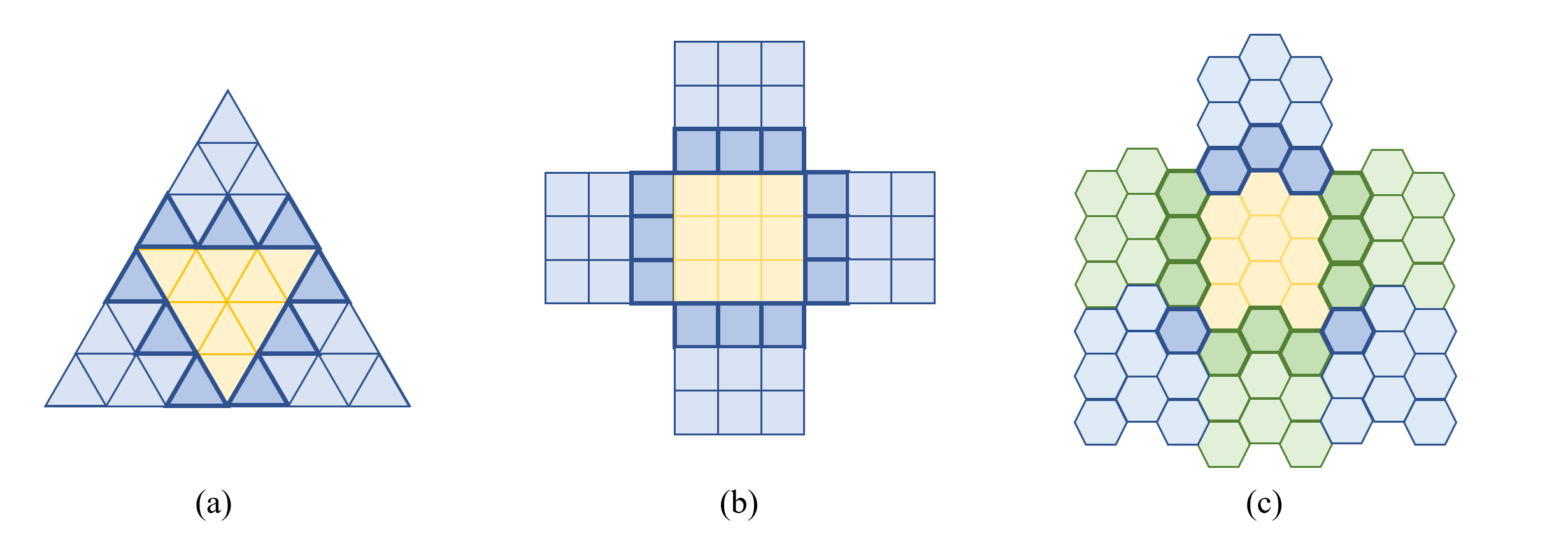
Figure 1: Panels (a), (b), and (c) illustrate examples of clusters, each differing in the values of $c$ and $r$. Specifically, these panels present clusters with $c=9$ and $r=3,4,$ and $6$, respectively. In each panel, the central cluster is emphasized in yellow, with its adjacent regions outlined by bold, darker edges. Upon examination, we find that the respective values of $\omega$ and the cardinality of $|\mathcal{N}_{\mathcal{C}_{j}}|$ are $\omega=1,3,3$ and $|\mathcal{N}_{\mathcal{C}_{j}}|=9,12,14$ for panels (a), (b), and (c), respectively.

We use three examples to show that spatially randomized designs generally yield estimators with lower MSEs compared to the global design; see also Figure 2 for numerical comparisons. The superiority of the spatially randomized designs becomes increasingly significant with large $R$.

Example 1

(Exchangeable) There exists some constant $0<\rho<1$ such that ${\mbox{cov}}(e_{\iota},e_{\iota^{\prime}})=\mathbb{I}(\iota=\iota^{\prime})+\rho\mathbb{I}(\iota\not=\iota^{\prime}).$ Then, we have ${{\operatorname{MSE}}\left(\widehat{{\tau}}^{i}\right)}/{{\operatorname{MSE}}\left(\widehat{{\tau}}^{g}\right)}\lesssim(r+1)^{2}/[1+\rho(R-1)]$.

Example 2

(Exponential-decay) Let $({x}_{\iota},{y}_{\iota})\in(0,1)^{2}$ denote the coordinates of the center of the $\iota$th region after scaling. Additionally, let $d_{\iota\iota^{\prime}}=\left\{({x}_{\iota}-{x}_{\iota^{\prime}})^{2}+({y}_{\iota}-{y}_{\iota^{\prime}})^{2}\right\}^{1/2}/2$ denote the spatial distance between $(x_{\iota},y_{\iota})$ and $(x_{\iota^{\prime}},y_{\iota^{\prime}})$. Assume there exists some $0<\rho<1$ such that ${\mbox{cov}}(e_{\iota},e_{\iota^{\prime}})=\rho^{d_{\iota\iota^{\prime}}}.$ Then, there exists some $0<\delta\leq\sqrt{2}$ such that ${{\operatorname{MSE}}\left(\widehat{{\tau}}^{i}\right)}/{{\operatorname{MSE}}\left(\widehat{{\tau}}^{g}\right)}\lesssim(1+r)^{2}/[1+(R-1)\rho^{\delta}]$.

Example 3

($d$-dependent) There exist some constant $0<\rho<1$ such that ${\mbox{cov}}(e_{\iota},e_{\iota^{\prime}})=\mathbb{I}(\iota=\iota^{\prime})+(\rho-\frac{|\iota-\iota^{\prime}|}{R})\mathbb{I}(|\iota-\iota^{\prime}|\leq\rho R).$ Then, we have ${{\operatorname{MSE}}\left(\widehat{{\tau}}^{i}\right)}/{{\operatorname{MSE}}\left(\widehat{{\tau}}^{g}\right)}\lesssim(1+r)^{2}/[1+(1-\rho)\rho^{2}R]$.

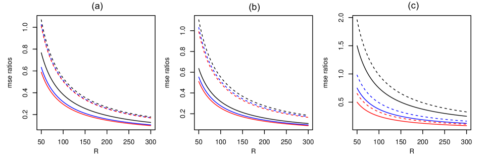
Figure 2: The figure illustrates the MSE ratios ${\operatorname{MSE}}(\widehat{\tau}^{i})/{\operatorname{MSE}}(\widehat{\tau}^{g})$ (solid lines) and ${\operatorname{MSE}}(\widehat{\tau}^{c})/{\operatorname{MSE}}(\widehat{\tau}^{g})$ with $c=9$ (dashed lines) across three distinct scenarios: Panel (a) corresponds to Example 1, Panel (b) to Example 2, and Panel (c) to Example 3. The urban area is segmented into uniform squares with $r=4$, and the total number of regions $R$ spans from $50$ to $300$. The black, blue, and red lines represent the MSE ratios for hyperparameter $\rho$ values of $0.3,0.6,$ and $0.9$, respectively, as detailed in Examples 1-3.

Semiparametric estimators. We next proceed to study the properties of doubly robust estimators. For the sake of brevity, we concentrate on scenarios where $p_{\iota}=p^{(j)}=p$ for all $\iota$ and $j$, meaning that the randomization probabilities are uniform across both spatially randomized designs. The subsequent theorem elucidates the MSEs of the three estimators.

Theorem 2

Suppose that CA holds and $p_{\iota}=p^{(j)}=p$ for any $\iota$ and $j$. Then, we have

$${\operatorname{MSE}}(\widehat{\tau}_{DR}^{g}) =\frac{1}{N}\sigma_{O}^{2}+\frac{1}{Np(1-p)}\sum_{\iota=1}^{R}\sum_{\iota^{\prime}=1}^{R}{\mathbb{V}}_{\iota\iota^{\prime}}+O\Big{[}\frac{R}{Np(1-p)}\sum_{\iota=1}^{R}\delta_{N,\iota}^{2}\Big{]},$$

$${\operatorname{MSE}}(\widehat{\tau}_{DR}^{i}) =\frac{1}{N}\sigma_{O}^{2}+\frac{1}{N}\sum_{\iota}\sum_{\iota^{\prime}}\Big{(}\frac{1}{p^{n_{\iota\iota^{\prime}}}}+\frac{1}{(1-p)^{n_{\iota\iota^{\prime}}}}\Big{)}{\mathbb{V}}_{\iota\iota^{\prime}}\mathbb{I}(n_{\iota\iota^{\prime}}>0)+O\Big{[}\frac{r^{2}}{N}\Big{(}\frac{1}{p^{r+1}}+\frac{1}{(1-p)^{r+1}}\Big{)}\sum_{\iota=1}^{R}\delta_{N,\iota}^{2}\Big{]},$$

$${\operatorname{MSE}}(\widehat{\tau}_{DR}^{c}) =\frac{1}{N}\sigma_{O}^{2}+\frac{1}{N}\sum_{\iota}\sum_{\iota^{\prime}}\Big{(}\frac{1}{p^{m_{\iota\iota^{\prime}}}}+\frac{1}{(1-p)^{m_{\iota\iota^{\prime}}}}\Big{)}{\mathbb{V}}_{\iota\iota^{\prime}}\mathbb{I}(m_{\iota\iota^{\prime}}>0)+O\Big{[}\frac{1}{Np(1-p)}\sum_{j=1}^{m}|\mathcal{C}_{j}^{0}|\sum_{\iota\in\mathcal{C}_{j}^{0}}\delta_{N,\iota}^{2}\Big{]}$$

$$+O\Big{[}\frac{m^{\prime}}{N}\Big{(}\frac{1}{p^{r^{\prime}+1}}+\frac{1}{(1-p)^{r^{\prime}+1}}\Big{)}\sum_{j=1}^{m}|\partial\mathcal{C}_{j}|\sum_{\iota\in\partial\mathcal{C}_{j}}\delta_{N,\iota}^{2}\Big{]}.$$

where $n_{\iota\iota^{\prime}}=|(\mathcal{N}_{\iota}\cup\{\iota\})\cap(\mathcal{N}_{\iota^{\prime}}\cup\{\iota^{\prime}\})|$, $m_{\iota\iota^{\prime}}=\sum_{k=1}^{m}\mathbb{I}((\mathcal{N}_{\iota}\cup\{\iota\})\cap\mathcal{C}_{k}\neq\emptyset,(\mathcal{N}_{\iota^{\prime}}\cup\{\iota^{\prime}\})\cap\mathcal{C}_{k}\neq\emptyset)$, $m^{\prime}=\max_{k}|\{k^{\prime}:\mathcal{N}_{\mathcal{C}_{k}}\cap\mathcal{N}_{\mathcal{C}_{k^{\prime}}}\neq\emptyset\}|$, $\sigma_{O}^{2}={\mbox{Var}}\left\{\sum_{\iota=1}^{R}[h_{\iota}(1,1,O_{t,\iota},\overline{O}_{t,\iota})-h_{\iota}(0,0,O_{t,\iota},\overline{O}_{t,\iota})]\right\}$, and $\sigma_{N,\iota}^{2}=\max_{a\in\{0,1\}}\mathbb{E}|\widehat{h}^{(k)}_{\iota}(a,a,O_{t,\iota},\bar{O}_{t,\iota})-h_{\iota}(a,a,O_{t,\iota},\bar{O}_{t,\iota})|^{2}$.

The MSEs of the three estimators are primarily determined by the first two terms. The residual term, governed by the rate at which the estimated outcome regression function converges, decays to zero at a faster rate. Notably, the first term is shared across the MSEs of all three estimators, which is independent of the treatment. Nevertheless, the second term introduces a divergence in the MSEs of these estimators, which we will explore in detail in the following corollary.

Corollary 3

Suppose that conditions in Theorem 2 hold, $p=0.5$, the interference range $r$ is fixed and $R^{-1}\sum_{\iota=1}^{R}\delta_{N,\iota}^{2}\to 0$.

• Let $r$ and $\nu$ be defined as they are in Corollary 2. Then as $N\rightarrow\infty$,

  $$\frac{{\operatorname{MSE}}(\widehat{\tau}_{DR}^{i})-N^{-1}\sigma_{O}^{2}}{{\operatorname{MSE}}(\widehat{\tau}_{DR}^{g})-N^{-1}\sigma_{O}^{2}}\lesssim\frac{(r+1)^{2}2^{r}}{\nu}.$$ (11)

• Let $r_{c}$ be the maximum number of adjacent clusters of a region and $\mathcal{R}_{1}$ be the index set of regions which are adjacent to more than two clusters. Denote $\mathcal{R}=\{1,2,\ldots,R\}$ as the index set of all regions, $\nu_{1}=\sum_{\iota}\sum_{\iota^{\prime}}{\mathbb{V}}_{\iota\iota^{\prime}}/\sum_{\iota\in\mathcal{R}_{1}}{\mathbb{V}}_{\iota\iota}$ and $\nu_{2}=\sum_{\iota}\sum_{\iota^{\prime}}{\mathbb{V}}_{\iota\iota^{\prime}}/\sum_{\iota\in\mathcal{R}/\mathcal{R}_{1}}{\mathbb{V}}_{\iota\iota}$. Then, we have

  $$\frac{N\cdot{\operatorname{MSE}}(\widehat{{\tau}}_{DR}^{c})-\sigma_{O}^{2}}{N\cdot{\operatorname{MSE}}(\widehat{{\tau}}_{DR}^{g})-\sigma_{O}^{2}}=O\left(\frac{cr\cdot r_{c}\cdot 2^{r_{c}}}{\nu_{1}}+\frac{cr}{\nu_{2}}\right).$$ (12)

With a constant interference range, the first ratio in (11) is bounded at $O(R^{-1})$. However, it will grow exponentially fast with $r$ due to the application of importance sampling (IS) $\mathbb{I}(\overline{A}_{t,\iota}=a)/{\mathbb{P}}(\overline{A}_{t,\iota}=a)$ in (8), a phenomenon we term the curse of spatial interference. This highlights a drawback of the individual-randomization design. In practical applications, this challenge can be alleviated by setting a lower bound on the denominator ${\mathbb{P}}(\overline{A}_{t,\iota}=a)$.

Another approach to address the curse of spatial interference is to adopt the cluster-level randomization, as indicated in point (ii) of Corollary 3. The advantage of this method is highlighted by the fact that, within each cluster, all internal points and their adjacent areas receive the same treatment. Thus, the curse of spatial interference is largely restricted to the cluster boundaries, which cover a much smaller area compared to the interiors, especially in larger clusters. Specifically, the first term on the right-hand side (RHS) of (12) represents the ratio of ${\operatorname{MSE}}(\widehat{\tau}^{c}_{DR})$, summed across all edge regions of the clusters (regions in $\mathcal{R}_{1}$), to ${\operatorname{MSE}}(\widehat{\tau}^{g}_{DR})$. The second term reflects the ratio of ${\operatorname{MSE}}(\widehat{\tau}^{c}_{DR})$, aggregated across all regions in $\mathcal{R}/\mathcal{R}_{1}$, to ${\operatorname{MSE}}(\widehat{\tau}^{g}_{DR})$, notably without the multiplication factor $2^{r_{c}}$. These ratios can be significantly lower than the RHS of (11) for two reasons: (i) $r_{c}$, the cluster-level interference range, can be much smaller than $r$. For example, in the scenarios illustrated in Figure 1, while $r$ is 3, 4, and 6, $r_{c}$ is only 3, 3, and 4, respectively. (ii) The second term in (12) is substantially smaller than that in (11), a discrepancy due to the scaling factor $R^{-1}\sum_{j=1}^{m}|\partial\mathcal{N}_{\mathcal{C}_{j}}|$, which reflects the much smaller proportion of boundary regions compared to interior ones.

2.5 Testing power in the nondynamic setting

In this section, we discuss how to construct the associated test statistics and analyze the influence of various designs on the power of these tests. We begin with the asymptotic normality of aforementioned estimators.

Theorem 3

When the conditions of Corollaries 2 and 3 hold, we have

• there exist constants $v^{g}$, $v^{i}$ and $v^{c}$ such that as $N\rightarrow\infty$,

  $$\sqrt{N(v^{g})^{-1}}\left(\widehat{{\tau}}^{g}-{{\tau}}\right)\overset{d}{\longrightarrow}N(0,1),\ \sqrt{N(v^{i})^{-1}}\left(\widehat{{\tau}}^{i}-{{\tau}}\right)\overset{d}{\longrightarrow}N(0,1),\ \sqrt{N(v^{c})^{-1}}\left(\widehat{{\tau}}^{c}-{{\tau}}\right)\overset{d}{\longrightarrow}N(0,1);$$

• there exist constants $v_{DR}^{g}$, $v_{DR}^{i}$ and $v_{DR}^{c}$ such that as $N\rightarrow\infty$,

  $$\sqrt{N(v_{DR}^{g})^{-1}}\Big{(}\widehat{{\tau}}_{DR}^{g}-{\tau}\Big{)}\overset{d}{\longrightarrow}N(0,1),\sqrt{N(v_{DR}^{i})^{-1}}\Big{(}\widehat{{\tau}}_{DR}^{i}-{\tau}\Big{)}\overset{d}{\longrightarrow}N(0,1),\sqrt{N(v_{DR}^{c})^{-1}}\Big{(}\widehat{{\tau}}_{DR}^{c}-{\tau}\Big{)}\overset{d}{\longrightarrow}N(0,1).$$

Conclusion (3.1) in Theorem 3 is a direct application of the asymptotic normality of the OLS estimator whereas (3.2) extends Theorem 5.1 in Chernozhukov et al. (2018) to settings with spatial interference. We next discuss the variance estimation. For the parametric model, it is straightforward to establish the sandwich estimators of the variances. Specifically, let $\widehat{e}_{t,\iota}^{g}$, $\widehat{e}_{t,\iota}^{i}$ and $\widehat{e}_{t,\iota}^{c}$ be the estimated residuals under the global, individual-randomized and cluster-randomized designs, respectively. Denote $\widehat{{\mathbb{V}}}_{\iota\iota^{\prime}}^{g}=N^{-1}\sum_{t=1}^{N}\widehat{e}_{t,\iota}^{g}\widehat{e}_{t,\iota^{\prime}}^{g}$, $\widehat{{\mathbb{V}}}_{\iota\iota^{\prime}}^{i}=N^{-1}\sum_{t=1}^{N}\widehat{e}_{t,\iota}^{i}\widehat{e}_{t,\iota^{\prime}}^{i}$ and $\widehat{{\mathbb{V}}}_{\iota\iota^{\prime}}^{c}=N^{-1}\sum_{t=1}^{N}\widehat{e}_{t,\iota}^{c}\widehat{e}_{t,\iota^{\prime}}^{c}$. Then the consistent sandwich estimators of ${\mbox{Var}}(\widehat{\tau}^{g})$, ${\mbox{Var}}(\widehat{\tau}^{i})$ and ${\mbox{Var}}(\widehat{\tau}^{c})$ are, respectively,

$$\widehat{{\mbox{Var}}}(\widehat{\tau}^{g})=\sum_{\iota=1}^{R}\sum_{\iota^{\prime}=1}^{R}u_{3}\left\{\sum_{t=1}^{N}Z_{t,\iota}^{g}\left(Z_{t,\iota}^{g}\right)^{\top}\right\}^{-1}\left\{\widehat{{\mathbb{V}}}_{\iota\iota^{\prime}}^{g}\sum_{t=1}^{N}Z_{t,\iota}^{g}\left(Z_{t,\iota^{\prime}}^{g}\right)^{\top}\right\}\left\{\sum_{t=1}^{N}Z_{t,\iota^{\prime}}^{c}\left(Z_{t,\iota^{\prime}}^{g}\right)^{\top}\right\}^{-1}u_{3}^{\top},$$

$$\widehat{{\mbox{Var}}}(\widehat{\tau}^{i})=\sum_{\iota=1}^{R}\sum_{\iota^{\prime}=1}^{R}u_{34}\left(\sum_{t=1}^{N}Z_{t,\iota}Z_{t,\iota}^{\top}\right)^{-1}\left\{\widehat{{\mathbb{V}}}_{\iota\iota^{\prime}}^{i}\sum_{t=1}^{N}Z_{t,\iota}Z_{t,\iota^{\prime}}^{\top}\right\}\left(\sum_{t=1}^{N}Z_{t,\iota^{\prime}}Z_{t,\iota^{\prime}}^{\top}\right)^{-1}u_{34}^{\top},$$

$$\widehat{{\mbox{Var}}}(\widehat{\tau}^{c})=\sum_{\iota=1}^{R}\sum_{\iota^{\prime}=1}^{R}u_{\iota}^{c}\left\{\sum_{t=1}^{N}Z_{t,\iota}^{c}\left(Z_{t,\iota}^{c}\right)^{\top}\right\}^{-1}\left\{\widehat{{\mathbb{V}}}_{\iota\iota^{\prime}}^{c}\sum_{t=1}^{N}Z_{t,\iota}^{c}\left(Z_{t,\iota^{\prime}}^{c}\right)^{\top}\right\}\left\{\sum_{t=1}^{N}Z_{t,\iota^{\prime}}^{c}\left(Z_{t,\iota^{\prime}}^{c}\right)^{\top}\right\}^{-1}(u_{\iota^{\prime}}^{c})\top.$$

For the doubly robust estimators, ${\mathbb{V}}_{\iota\iota^{\prime}}$ can be estimated similarly. Let ${\Delta}_{t\iota}=[\widehat{h}_{\iota}(1,1,O_{t,\iota},\overline{O}_{t,\iota})-\widehat{h}_{\iota}(0,0,O_{t,\iota},\overline{O}_{t,\iota})]$ and $\overline{\Delta}_{t\iota}=N^{-1}\sum_{t=1}^{N}{\Delta}_{t\iota}$. The remaining term $\sigma_{O}^{2}$ can be estimated by $N^{-1}\sum_{t=1}^{N}\{{\Delta}_{t\iota}-\overline{{\Delta}}_{t\iota}\}^{2}$. One can also use the bootstrap method to obtain the consistent estimators of the variances.

To illustrate the testing performances of different designs, we consider the following local alternative hypotheses

$$H_{0}:{\tau}=0\text{\ \ V.S.\ \ }H_{1}:{\tau}=h/\sqrt{N}.$$ (13)

Given an asymptotic normal ATE estimate $\widehat{\tau}$ along with the corresponding consistent variance estimate $\widehat{\mbox{Var}}(\widehat{\tau})$, a popular test statistic for the hypotheses in (13) is the Wald statistic

$$\widehat{T}=\frac{\widehat{\tau}}{\sqrt{\widehat{\mbox{Var}}(\widehat{\tau})}}.$$

Let $c_{\delta}$ be the $(1-\delta)$th quantile of the standard Gaussian distribution and $\Phi(\cdot)$ be the cumulative density function. Regarding the hypotheses in (13), the null hypothesis is rejected when $\widehat{T}\geq c_{\delta}$. When the null hypothesis holds, as the sample size $N$ approaches infinity, $\widehat{T}$ converges to the standard Gaussian distribution, and hence $P\left(T\geq c_{\delta}\right)\rightarrow\delta$. When the alternative hypothesis is true, we have the following conclusion.

Corollary 4

Suppose that the conditions of Corollaries 2 and 3 hold, each $\mathbb{V}_{\iota\iota^{\prime}}$ is bounded from above and $\sum_{\iota\iota^{\prime}}\mathbb{V}_{\iota\iota^{\prime}}/R^{2}$ is bounded from below. Under the alternative hypothesis, as $N\rightarrow\infty$,

• the sufficient and necessary conditions for $P\left(\widehat{T}^{g}\geq c_{\delta}\right)\rightarrow 1,P\left(\widehat{T}^{i}\geq c_{\delta}\right)\rightarrow 1$ and $P\left(\widehat{T}^{c}\geq c_{\delta}\right)\rightarrow 1$ are $h\gg c_{\delta}R,$ $h\gg c_{\delta}r\sqrt{R},$ and $h\gg c_{\delta}(\sqrt{m}r+\sqrt{cR})$, respectively.

• the sufficient and necessary conditions for $P\left(\widehat{T}_{DR}^{g}\geq c_{\delta}\right)\rightarrow 1,P\left(\widehat{T}_{DR}^{i}\geq c_{\delta}\right)\rightarrow 1$ and $P\left(\widehat{T}_{DR}^{c}\geq c_{\delta}\right)\rightarrow 1$ are $h\gg c_{\delta}\sqrt{\sigma_{O}^{2}+R^{2}},h\gg c_{\delta}\sqrt{\sigma_{O}^{2}+r2^{r}R}$ and $h\gg c_{\delta}\{\sigma_{O}^{2}+|\mathcal{R}_{1}|crr_{c}2^{r_{c}}+(R-|\mathcal{R}_{1}|)cr\}^{1/2}$, respectively.

In conclusion (4.1), when $r$ is a constant and the cluster size $c\ll R$, then $\{r\sqrt{R},\sqrt{m}r+\sqrt{cR}\}\ll R$ as $R\to\infty$. In conclusion (4.2), when $r$ and $r_{c}$ are constants, $c\ll R$ and the number of edge regions $|\mathcal{R}_{1}|\ll R$ (for instance, $c=O(R^{\delta})$ for some $0<\delta<1$), it holds that $\{r2^{r}R,|\mathcal{R}_{1}|crr_{c}2^{r_{c}}+(R-|\mathcal{R}_{1}|)cr\}\ll R^{2}$. In other words, under mild conditions, the power of test statistics under spatially randomized designs achieves 1 more rapidly than under the global design, and this advantage grows as the number of regions $R$ increases. Consequently, spatially randomized designs lead to more efficient testing results, particularly in the presence of weaker signals.

3 Dynamic Setting

In this section, we consider scenarios where within each day, each spatial unit receives $M$ (possibly different) treatments over time. The data are represented as $\left\{\left(A_{i\iota t},O_{i\iota t},Y_{i\iota t}\right)\right\}_{1\leq i\leq N,1\leq\iota\leq R,1\leq t\leq M}$ where $i$ indexes the $i$th day, $\iota$ indexes the $\iota$the region, $t$ indexes the $t$th time interval, corresponding to i.i.d. copies of $\{\left(A_{\iota t},O_{\iota t},Y_{\iota t}\right)\}_{1\leq\iota\leq R,1\leq t\leq M}$. To simplify the presentation, we have chosen not to employ the potential outcome framework to formulate the causal estimand. Readers who are interested in exploring the potential outcomes approach may refer to the works by Luckett et al. (2019) and Shi et al. (2023). The ATE in this context is given by:

$${\tau}=\sum_{t=1}^{M}\sum_{\iota=1}^{R}[{\mathbb{E}}_{1}(Y_{i\iota R})-{\mathbb{E}}_{0}(Y_{i\iota R})],$$

where ${\mathbb{E}}_{1}$ and ${\mathbb{E}}_{0}$ denote the expectation assuming that treatments are assigned according to two non-dynamic policies: consistently set to 1 and consistently set to 0, respectively. In settings with multiple decision stages, past interventions may influence current variables, thereby indirectly impacting current outcomes. This carryover effects adds complexity to both the estimation process and theoretical analysis.

3.1 Parametric and semiparametric modeling

For parametric modeling, in addition to the outcome regression model, we posit another first-order autoregression model for the observational variable, yielding the following pair of models:

$$\begin{split}&Y_{i\iota t}=\alpha_{\iota t}+O_{i\iota t}^{\top}\beta_{\iota t}+\gamma_{\iota t}A_{i\iota t}+\theta_{\iota t}\overline{A}_{i\mathcal{N}_{\iota t}}+e_{i\iota t},\\ &O_{i\iota,t+1}=\Lambda_{\iota t}+B_{\iota t}O_{i\iota t}+\Gamma_{\iota t}A_{i\iota t}+\Theta_{\iota t}\overline{A}_{i\mathcal{N}_{\iota t}}+E_{i\iota t},\end{split}$$ (14)

where $\Lambda_{\iota t},\Gamma_{\iota t},\Theta_{\iota t}\in\mathbb{R}^{d}$, $B_{\iota t}\in\mathbb{R}^{d\times d}$ and $\{e_{i\iota t},E_{i\iota t}\}$ are i.i.d. copies of $\{e_{\iota t},E_{\iota t}\}$ which are independent of $\{O_{i\iota t}\}$ and satisfy ${\mathbb{E}}(e_{\iota t})=0$, ${\mbox{cov}}(e_{\iota t},e_{\iota^{\prime}t^{\prime}})={\mathbb{V}}_{\iota\iota^{\prime}t}^{e}\mathbb{I}\{t=t^{\prime}\}$, ${\mathbb{E}}(E_{\iota t})=0$, and ${\mbox{cov}}(E_{\iota t},E_{\iota^{\prime}t^{\prime}})={\mathbb{V}}_{\iota\iota^{\prime}t}^{E}\mathbb{I}\{t=t^{\prime}\}$, respectively, and for all $\iota$, ${e_{\iota t}}$ and ${E_{\iota t}}$ are independent over $t$. For the global design where $A_{i\iota t}=A_{it}$ for any $\iota$, model (14) degenerates to

$$Y_{i\iota t}=\alpha_{\iota t}+O_{i\iota t}^{\top}\beta_{\iota t}+\gamma_{\iota t}^{g}A_{it}+e_{i\iota t},$$ (15)

$$O_{i\iota,t+1}=\Lambda_{\iota t}+B_{\iota t}O_{i\iota t}+\Gamma_{\iota t}^{g}A_{it}+E_{i\iota t},$$

where $\gamma_{\iota t}^{g}=\gamma_{\iota t}+\theta_{\iota t}$ and $\Gamma_{\iota t}^{g}=\Gamma_{\iota t}+\Theta_{\iota t}$.

We now turn our focus to estimating ${\tau}$ within the framework of models (14) and (15). We first present the subsequent proposition.

Proposition 1

Define $c_{\iota t}^{\top}$ as $\sum_{k=t+1}^{M}\beta_{\iota k}^{\top}\left(\prod_{j=t+1}^{k-1}B_{\iota j}\right)$. Under models (14) and (15), the ATE can be expressed as

$${\tau}=\sum_{\iota=1}^{R}\sum_{t=1}^{M}\Big{(}\gamma_{\iota t}^{g}+c_{\iota t}^{\top}\Gamma_{\iota t}^{g}\Big{)}=\sum_{\iota=1}^{R}\sum_{t=1}^{M}\Big{\{}\gamma_{\iota t}+\theta_{\iota t}+c_{\iota t}^{\top}\big{(}\Gamma_{\iota t}+\Theta_{\iota t}\big{)}\Big{\}}.$$ (16)

Proposition 1 shows that the ATE consists of two components: the initial terms $\gamma_{\iota t}^{c}=\gamma_{\iota t}+\theta_{\iota t}$ represents the direct effect of $A_{t}$ on the immediate outcomes, whereas the last term $c_{\iota t}^{\top}\Gamma_{\iota t}^{g}=c_{\iota t}^{\top}(\Gamma_{\iota t}+\Theta_{\iota t})$ corresponds to the indirect effect, measuring the delayed treatment effect on future outcomes through $O_{t+1}$. Analogous to the nondynamic setting, one can derive OLS estimators for the regression coefficients and plug-in them into (16) to obtain the estimated $\tau$. To save space, we do not detail the estimating procedure again.

For semiparametric modeling, we follow the double reinforcement learning method (DRL, Kallus and Uehara 2020) and model the data using a (time-varying) Markov decision process (MDP, Puterman 2014). The key feature of an MDP is the Markov assumption, given $\bm{O}_{t}=\{O_{\iota t}\}_{\iota}$ and $\bm{A}_{t}=\{A_{\iota t}\}_{\iota}$, the immediate outcomes $\bm{Y}_{t}=\{Y_{\iota t}\}_{\iota}$ and future observations $\bm{O}_{t+1}$ are independent of the past data history $\{(\bm{O}_{j},\bm{A}_{j},\bm{Y}_{j}):j<t\}$. For $a\in\{0,1\}$, we define the Q-function

$$Q_{\iota t}^{a}(\bm{O}_{t},\bm{A}_{t})=\sum_{k=t}^{M}{\mathbb{E}}_{a}(Y_{\iota k}|\bm{O}_{t},\bm{A}_{t})\ \text{ for }\iota=1,\ldots,R,1\leq t\leq M.$$

Additionally, we define $\mu_{\iota t}$ as the ratio of the probability mass/density function of the observation-treatment pair between the target policy (which sets the treatments to 1 or 0 at all time) and the behavior policy (which generates the offline data) at time $t$, i.e.,

$$\mu_{\iota t}^{a}(\bm{O}_{t},\bm{A}_{t})=\frac{[\prod_{\iota}\mathbb{I}(A_{\iota t}=a)]p_{a}(\bm{O}_{t})}{{\mathbb{P}}(\cap_{\iota}\{A_{\iota t}=a\}|\bm{O}_{t})p_{b}(\bm{O}_{t})},\quad a\in\{0,1\},$$

where $p_{a}$ and $p_{b}$ denote the density functions of $\bm{O}_{t}$ under the target policy and the behavior policy respectively. The resulting DRL estimator is given by

$$\widetilde{\tau}_{DRL}=\frac{1}{N}\sum_{a=0}^{1}(-1)^{a+1}\sum_{i=1}^{N}\sum_{\iota=1}^{R}\Big{\{}Q_{\iota 1}^{a}(\bm{O}_{i1},a)+\sum_{t=1}^{M}\mu_{\iota t}^{a}(\bm{O}_{it},\bm{A}_{it})[Y_{i\iota t}+Q_{\iota t+1}^{a}(\bm{O}_{it+1},a)-Q_{\iota t}^{a}(\bm{O}_{it},\bm{A}_{it})]\Big{\}}.$$

The key challenge in constructing $\widetilde{\tau}_{DRL}$ lies in the accurate estimation of $Q_{\iota t}^{a}$ and $\mu_{\iota t}^{a}$. Given their inputs are high-dimensional, specifically $2Rd$-dimensional, it is challenging to consistently estimate these functions. Moreover, parallel to the curse of horizon phenomenon detailed by Liu et al. (2018), the variance of $\widetilde{\tau}_{DRL}$ grows exponentially fast with respect to the input dimension of $\mu_{\iota t}^{a}$. To address both challenges, we adopt the mean-field approximation to effectively reduce the input dimensions of $Q_{\iota t}^{a}$ and $\mu_{\iota t}^{a}$ (Yang et al. 2018, Shi et al. 2022). Specifically, let $m_{\iota}$ be a known function of local observations and actions related to the $\iota$th region for each $\iota$. For example, it might take the form of simple averages derived from the observations and actions of the $\iota$th region’s neighbouring regions. The mean field assumption assumes (i) both $Q_{\iota t}^{a}(\bm{O}_{t},\bm{A}_{t})$ and the reward function ${\mathbb{E}}(Y_{\iota t}|\bm{O}_{t},\bm{A}_{t})$ are functions of $X_{\iota t}=(O_{\iota t},{A}_{\iota t},m_{\iota}(\bm{O}_{t},\bm{A}_{t}))$ only; (ii) $O_{\iota t+1}$ and $m_{\iota}(\bm{O}_{t},\bm{A}_{t})$ are conditionally independent of the past observation-action pair given $X_{\iota t}$. These assumptions can be verified via state-of-the-art Markov tests (Chen and Hong 2012, Shi et al. 2020, Zhou et al. 2023) or conditional independence type tests (Bergsma 2004, Zhang et al. 2011, Shah and Peters 2020, Shi et al. 2021). Under these assumptions, it can be shown that $\widetilde{\tau}_{DRL}$ is unbiased to the following (Shi et al. 2022)

$$\widehat{\tau}_{DRL}=\frac{1}{N}\sum_{a=0}^{1}(-1)^{a+1}\sum_{i=1}^{N}\sum_{\iota=1}^{R}\Big{\{}Q_{\iota 1}^{a}(X_{i\iota t}^{a})+\sum_{t=1}^{M}\mu_{\iota t}^{a}(X_{i\iota t})[Y_{i\iota t}+Q_{\iota t+1}^{a}(X_{i\iota t+1}^{a})-Q_{\iota t}^{a}(X_{i\iota t})]\Big{\}},$$

where $X_{\iota t}^{a}$ is a shorthand for $(O_{\iota t},a,m_{\iota}(\bm{O}_{t},a))$ and $\mu_{\iota t}^{a}$ denotes the ratio of the probability mass/density function of $X_{\iota t}$ between the target policy and the behavior policy. Different from $\widetilde{\tau}_{DRL}$, the Q-function and the ratio in $\widehat{\tau}_{DRL}$ rely only on $X_{\iota t}$ (or $X_{\iota t}^{a}$) whose dimension can be much smaller than that of $\bm{O}_{t}$ and $\bm{A}_{t}$.

It remains to estimate $Q_{\iota t}^{a}$ and $\mu_{\iota t}^{a}$ to compute $\widehat{\tau}_{DRL}$. To estimate $Q_{\iota t}^{a}$, we employ backward induction (Murphy 2003). Specifically, we begin by estimating $Q_{\iota M}^{a}(X_{\iota M})={\mathbb{E}}(Y_{\iota M}|X_{\iota M})$. Let $\widehat{Q}_{\iota M}^{a}$ denote the resulting estimator. We next recursively estimate $Q_{\iota t}^{a}(X_{\iota t})={\mathbb{E}}[Y_{\iota t}+\widehat{Q}_{\iota t+1}^{a}(X_{\iota t+1}^{a})|X_{\iota t}]$ for $t=M-1,M-2,\cdots,1$ and construct these estimators $\{\widehat{Q}_{\iota t}^{a}\}_{t}$ via nonparametric regression (e.g., kernel smoothing or splines). To estimate $\mu_{\iota t}^{a}$, we employ minimax learning (Liu et al. 2018, Uehara et al. 2020). To save space, we relegate the detailed implementation to Section 2 of the supplementary article.

Finally, similar to the contextual bandit setting, we employ data-splitting and cross-fitting to construct $\widehat{\tau}_{DRL}$. We summarize our procedure in Algorithm 2.

Algorithm 2 Doubly reinforcement learning in dynamic settings

Data $\{(O_{i,\iota,t},A_{i,\iota,t},Y_{i,\iota,t})\}_{i,\iota,t}$ collected from a given design.

1: Split all data trajectories into $K$ ($K\geq 2$) non-overlapped subsets, each with an equal size. Let $\mathcal{D}_{k}$ denote the indices of days that belong to the $k$th data subset where $k=1,2,\ldots,K$.

2: For $k=1,\ldots,K$, $a\in\{0,1\}$, $1\leq t\leq M$ and $1\leq\iota\leq R$, compute $\widehat{\mu}_{\iota t}^{a,(k)}$ and $\widehat{Q}_{\iota t}^{a,(k)}$ based on data trajectories $\{1,\ldots,n\}\backslash\mathcal{D}_{k}$.

3: Set

$$\widehat{\tau}_{DRL}=\frac{1}{N}\sum_{a=0}^{1}(-1)^{a+1}\sum_{k=1}^{K}\sum_{i\in\mathcal{D}_{k}}\sum_{\iota=1}^{R}\Big{\{}\widehat{Q}_{\iota 1}^{a,(k)}(X_{i\iota t}^{a})+\sum_{t=1}^{M}\widehat{\mu}_{\iota t}^{a,(k)}(X_{i\iota t})[Y_{i\iota t}+\widehat{Q}_{\iota t+1}^{a,(k)}(X_{i\iota t+1}^{a})-\widehat{Q}_{\iota t}^{a,(k)}(X_{i\iota t})]\Big{\}}.$$

3.2 Estimation accuracy in the dynamic setting

In this section, we compare the following three spatial designs in the dynamic setting:

• Global design: all regions receive the same treatment at each time, i.e., $A_{\iota t}=A_{t}$ for any $\iota$.

• Individual-randomized design: the sequence of treatments for each region is independently generated. In other words, for any two regions $\iota$ and $\iota^{\prime}$, we have $\{A_{\iota t}\}_{t}\mathchoice{\mathrel{\hbox to0.0pt{$\displaystyle\perp$\hss}\mkern 2.0mu{\displaystyle\perp}}}{\mathrel{\hbox to0.0pt{$\textstyle\perp$\hss}\mkern 2.0mu{\textstyle\perp}}}{\mathrel{\hbox to0.0pt{$\scriptstyle\perp$\hss}\mkern 2.0mu{\scriptstyle\perp}}}{\mathrel{\hbox to0.0pt{$\scriptscriptstyle\perp$\hss}\mkern 2.0mu{\scriptscriptstyle\perp}}}\{A_{\iota^{\prime}t}\}_{t}$.

• Cluster-randomized design: all regions are partitioned into $m$ clusters. Each cluster’s regions receive identical treatments at every time step, and treatment sequences are independently generated across different clusters.

Additionally, since treatments are sequentially assigned over time, we incorporate the spatial designs with the following temporal designs:

• Constant design: each region receives the same treatment at each day. In other words, we have $A_{\iota 1}=A_{\iota 2}=\cdots=A_{\iota M}$ for each $1\leq\iota\leq R$.

• Independent design: within each day, the treatments for each region at every time point are independently generated. Thus, all $A_{\iota t}$s are independent for each $\iota$.

• Switchback design: for each region on each day, the initial treatment is randomly generated. The following treatment alternates with the previous one, resulting in a sequence where the treatments switch back and forth. Specifically, $A_{\iota 1}=1-A_{\iota 2}=A_{\iota 3}=1-A_{\iota 4}=\cdots$ for any $\iota$.

In settings with a single spatial unit, it has been shown that the constant design is optimal under standard MDP assumptions, i.e., the ATE under this design achieves the smallest MSE (Li et al. 2023). However, when the rewards are auto-correlated, the independent and switchback design could produce more efficient estimators (Luo et al. 2024). Additionally, the switchback design has been widely studied in the literature (see e.g., Hu and Wager 2022, Bojinov et al. 2023, Xiong et al. 2023). It has been frequently employed in practice.

We first compare different designs under the parametric model assumption (14). Let $\widehat{\tau}_{OLS}^{g},\widehat{\tau}_{OLS}^{i}$ and $\widehat{\tau}_{OLS}^{c}$ be the estimators under the global, individual- and cluster-randomized designs, respectively. We introduce the following noise quantity $u_{i\iota t}=c_{\iota t}^{\top}E_{i\iota t}+e_{i\iota t}$, where $c_{\iota t}$ is defined the same as in Proposition 1 and represents the delayed indirect effects. Let ${\mathbb{V}}_{\iota\iota^{\prime}t}^{u}$ denote ${\mbox{cov}}(u_{i\iota t},u_{i\iota^{\prime}t})$.

Theorem 4

Assume that either the constant design, the independent design, or the switchback design is implemented temporally.

• As $N\rightarrow\infty$, we have:

  $${\operatorname{MSE}}\left(\widehat{{\tau}}_{OLS}^{g}\right)-N^{-1}\sigma_{OLS}^{2}\asymp\frac{4}{N}\sum_{t=1}^{M}\sum_{\iota=1}^{R}\sum_{\iota^{\prime}=1}^{R}{\mathbb{V}}_{\iota\iota^{\prime}t}^{u},$$

  $${\operatorname{MSE}}\left(\widehat{{\tau}}_{OLS}^{i}\right)-N^{-1}\sigma_{OLS}^{2}\asymp\frac{4}{N}\sum_{t=1}^{M}\left\{\sum_{\iota=1}^{R}{\mathbb{V}}_{\iota\iota t}^{u}+2\sum_{\iota=1}^{R}\sum_{\iota^{\prime}\in\mathcal{N}_{\iota}}{\mathbb{V}}_{\iota\iota^{\prime}t}^{u}+\sum_{\iota,\iota^{\prime}=1}^{R}\left|\mathcal{N}_{\iota}\cap\mathcal{N}_{\iota^{\prime}}\right|{\mathbb{V}}_{\iota\iota^{\prime}t}^{u}\right\},$$

  $${\operatorname{MSE}}(\widehat{{\tau}}_{OLS}^{c})-N^{-1}\sigma_{OLS}^{2}\asymp\frac{4}{N}\sum_{t=1}^{M}\sum_{j=1}^{m}\left\{\sum_{\iota,\iota^{\prime}\in\mathcal{C}_{j}}{\mathbb{V}}_{\iota\iota^{\prime}t}^{u}+2\sum_{\iota\in\mathcal{C}_{j}}\sum_{\iota^{\prime}\in\mathcal{N}_{\mathcal{C}_{j}}}\omega_{\iota^{\prime}}n_{\iota^{\prime}}^{(j)}{\mathbb{V}}_{\iota\iota^{\prime}t}^{u}+\sum_{\iota,\iota^{\prime}\in\mathcal{N}_{\mathcal{C}_{j}}}\omega_{\iota}\omega_{\iota^{\prime}}n_{\iota}^{(j)}n_{\iota^{\prime}}^{(j)}{\mathbb{V}}_{\iota\iota^{\prime}t}^{u}\right\},$$

  where $\sigma_{OLS}^{2}$ represents the common part of the MSEs of the three estimators.

• Denote $\eta$ as $\sum_{t=1}^{M}\sum_{\iota=1}^{R}\sum_{\iota^{\prime}=1}^{R}\mathbb{V}_{\iota\iota^{\prime}t}^{u}/\sum_{t=1}^{M}\sum_{\iota=1}^{R}\mathbb{V}_{\iota\iota t}^{u}$, the MSE ratios are:

  $$\frac{N\cdot{\operatorname{MSE}}\left(\widehat{{\tau}}_{OLS}^{i}\right)-\sigma_{OLS}^{2}}{N\cdot{\operatorname{MSE}}\left(\widehat{{\tau}}_{OLS}^{g}\right)-\sigma_{OLS}^{2}}\lesssim\frac{(r+1)^{2}}{\eta}\quad\mbox{and}\quad\frac{N\cdot{\operatorname{MSE}}\left(\widehat{{\tau}}_{OLS}^{c}\right)-\sigma_{OLS}^{2}}{N\cdot{\operatorname{MSE}}\left(\widehat{{\tau}}_{OLS}^{g}\right)-\sigma_{OLS}^{2}}=O\left(\frac{\sum_{j=1}^{m}\sum_{\iota,\iota^{\prime}\in\mathcal{C}_{j}\cup\mathcal{N}_{\mathcal{C}_{j}}}{\mathbb{V}}_{\iota\iota^{\prime}}^{u}}{\sum_{\iota,\iota^{\prime}}{\mathbb{V}}_{\iota\iota^{\prime}}^{u}}\right).$$

The results in Theorem 4 are consistent with those in Theorem 1 and Corollary 2. The explicit expression of $\sigma_{OLS}^{2}$ is presented in Section 1.7 of the supplementary materials. We remark that if the indirect effects are weak, such that $\Gamma_{\iota t}=O(R^{-1/2})$ for any $\iota$ and $t$, or if for any $t$, $\{E_{i\iota t}\}_{\iota}$ are correlated only within the neighbors, then we have

$$\frac{\sigma_{OLS}^{2}}{N\cdot{\operatorname{MSE}}\left(\widehat{{\tau}}_{OLS}^{g}\right)-\sigma_{OLS}^{2}}=O\left(\frac{r^{2}}{R}\right).$$

Similar to Case 2 in the discussion of Corollary 2, When each $\mathbb{V}_{\iota\iota^{\prime}t}^{u}$ is bounded from above and $\sum_{\iota\iota^{\prime}}\mathbb{V}_{\iota\iota^{\prime}t}^{u}/R^{2}$ is bounded from below, we have the following results:

$$\frac{{\operatorname{MSE}}(\widehat{{\tau}}_{OLS}^{i})}{{\operatorname{MSE}}(\widehat{{\tau}}_{OLS}^{g})}=O\Big{(}\frac{r^{2}}{R}\Big{)}\quad\mbox{and}\quad\frac{{\operatorname{MSE}}(\widehat{{\tau}}_{OLS}^{c})}{{\operatorname{MSE}}(\widehat{{\tau}}_{OLS}^{g})}=O\Big{(}\frac{c}{R}+\frac{mr^{2}}{R^{2}}\Big{)}.$$

To compare the semiparametric estimators, we assume:

Assumption 1

For $1\leq\iota\leq R$, $1\leq t\leq M$ and $a=0,1$, the reward $Y_{\iota t}$ and the density ratio $\mu_{\iota t}^{a}$ are bounded; the estimators of the sample splitting procedure $\widehat{\mu}_{\iota t}^{a,(k)}$ and $\widehat{Q}_{\iota t}^{a,(k)}$ are finite.

Denote the DRL ATE estimators under the global, individual- and cluster-randomized designs as $\widehat{\tau}_{DRL}^{g},\widehat{\tau}_{DRL}^{i}$ and $\widehat{\tau}_{DRL}^{c}$, respectively. Define the noise term $u_{\iota t}=r_{\iota t}-{\mathbb{E}}(r_{\iota t}|O_{\iota t},A_{\iota t},m_{\iota}(\bm{O}_{\iota t},\bm{A}_{\iota t}))$ and let $C_{\iota_{1},\iota_{2},t}={\mbox{cov}}\{u_{\iota_{1},t},u_{\iota_{2},t}\}$ be its covariance. Then we have the following result in parallel to Theorem 2.

Theorem 5

Suppose that $m_{\iota}(\bm{O}_{t},\bm{A}_{t})=(|\mathcal{N}_{\iota}|^{-1}\sum_{k\in\mathcal{N}_{\iota}}O_{kt},|\mathcal{N}_{\iota}|^{-1}\sum_{k\in\mathcal{N}_{\iota}}A_{kt})$. Under the condition that $r$ is finite, and all elements in $\{C_{\iota_{1},\iota_{2},t}:1\leq\iota_{1},\iota_{2}\leq R,1\leq t\leq M\}$ are nonnegative with a substantial proportion distinctly greater than zero, the following results hold as $N\rightarrow\infty$:

$$\frac{N\cdot{\operatorname{MSE}}(\widehat{\tau}^{i}_{DRL})-\sigma_{DRL}^{2}}{N\cdot{\operatorname{MSE}}(\widehat{\tau}^{g}_{DRL})-\sigma_{DRL}^{2}}=O\left(\frac{r2^{r}}{R^{2}}\right)\quad\mbox{and}\quad\frac{N\cdot{\operatorname{MSE}}(\widehat{\tau}^{c}_{DRL})-\sigma_{DRL}^{2}}{N\cdot{\operatorname{MSE}}(\widehat{\tau}^{g}_{DRL})-\sigma_{DRL}^{2}}=O\left(\frac{cr\cdot r_{c}\cdot 2^{r_{c}}}{\nu_{1}}+\frac{cr}{\nu_{2}}\right),$$

where $\sigma_{DRL}^{2}={\mbox{Var}}\{\sum_{\iota=1}^{R}(Q_{\iota 1}(\bm{1}_{RM})-Q_{\iota 1}(\bm{0}_{RM}))\}$.

We now establish the asymptotic normality of the ATE estimators in a dynamic framework when $M$ remains finite.

Theorem 6

For models and ATE estimators discussed in this section, we have the following asymptotic normality results:

• when conditions of Theorem 4 hold, there exist constants $v_{OLS}^{g},v_{OLS}^{i},v_{OLS}^{c}$ such that as $N\rightarrow\infty$,

  $$\sqrt{N(v_{OLS}^{g})^{-1}}\Big{(}\widehat{{\tau}}_{OLS}^{g}-{\tau}\Big{)}\overset{d}{\longrightarrow}N(0,1),\ \sqrt{N(v_{OLS}^{i})^{-1}}\Big{(}\widehat{{\tau}}_{OLS}^{i}-{\tau}\Big{)}\overset{d}{\longrightarrow}N(0,1),\ \sqrt{N(v_{OLS}^{c})^{-1}}\Big{(}\widehat{{\tau}}_{OLS}^{c}-{\tau}\Big{)}\overset{d}{\longrightarrow}N(0,1);$$

• when the assumptions of Theorem 5 hold, there exist constants $v_{DRL}^{g},v_{DRL}^{i},v_{DRL}^{c}$ such that as $N\rightarrow\infty$,

  $$\sqrt{N(v_{DRL}^{g})^{-1}}\Big{(}\widehat{{\tau}}_{DRL}^{g}-{\tau}\Big{)}\overset{d}{\longrightarrow}N(0,1),\ \sqrt{N(v_{DRL}^{i})^{-1}}\Big{(}\widehat{{\tau}}_{DRL}^{i}-{\tau}\Big{)}\overset{d}{\longrightarrow}N(0,1),\ \sqrt{N(v_{DRL}^{c})^{-1}}\Big{(}\widehat{{\tau}}_{DRL}^{c}-{\tau}\Big{)}\overset{d}{\longrightarrow}N(0,1).$$

The first conclusion is derived from the asymptotic normality of OLS estimators, while the second is inferred from Theorem 19 in Shi et al. (2022). Consequently, consistent variance estimators can be acquired utilizing the bootstrap method. Similar to Section 2.5, with the asymptotic normality and consistent variance estimators, we can establish the Walt test statistics. Recalling that in Theorem 4 and 5, we have proved that the spatially randomized designs can produce estimators with smaller MSEs. Note that the testing power decreases with MSEs. We can deduce that spatially randomized designs can lead to testing statistics with higher powers.

4 Numerical Experiments

In this section, we conduct numerical experiments to validate the theoretical insights derived from Sections 2-3.

4.1 Simulation of the nondynamic setting

In this subsection, our initial numerical experiment focuses on a parametric regression model within a non-dynamic, single-stage framework. We create regions amounting to $R=36,81,144$, each fashioned into regular polygons with 3, 4, and 6 sides corresponding to $r=3,4,6$, respectively. For each configuration, we utilize clusters of equal size, specifically $|\mathcal{C}_{\iota}|=9$, leading to total cluster counts of $m=4,9,16$, as depicted in Figure 3. The covariate values $O_{t,\iota}$ are i.i.d, following a normal distribution $N(4,1)$.

We define $(\iota_{x},\iota_{y})$ as the coordinates of region $\iota$, both normalized to the interval $(0,1)$. The coefficients $\alpha_{\iota t}$ and $\beta_{\iota t}$ are determined as $\alpha_{\iota}=8+2\{f_{1}(\iota_{x})+g_{1}(\iota_{y})\}$ and $\beta_{\iota}=f_{2}(\iota_{x})+g_{2}(\iota_{y}),$ where $f_{1}(\cdot)$, $f_{2}(\cdot)$, $g_{1}(\cdot)$, and $g_{2}(\cdot)$ represent specific functions structured as $a_{0}+\sum_{k=1}^{K}\{a_{k}\cos(k\pi x)+b_{k}\sin(k\pi x)\}$, with coefficients $a_{0},a_{k},b_{k}$ randomly drawn from a uniform distribution over $[0,1]$ and $K$ set to 3. The effect coefficients $\{\gamma_{\iota}\}_{\iota}$ are generated according to the patterns of $\alpha_{\iota},\beta_{\iota}$, $\gamma_{\iota}=s_{y}\cdot{\alpha_{\iota}}/{\sum_{\iota}\alpha_{\iota}}$ and $\theta_{\iota}=s_{y}\cdot 0.6\cdot{\beta_{\iota}}/{\sum_{\iota}\beta_{\iota}}$, where $s_{y}$ is the signal strength defined as which corresponds to $100s\%$ improvement compared to the outcome of the control group. We simulate a range of $s=0,0.0025,0.005,0.0075,0.01,0.0125,0.015,0.0175,$ and $0.02$ with 500 replicates and $N=30$ observations.

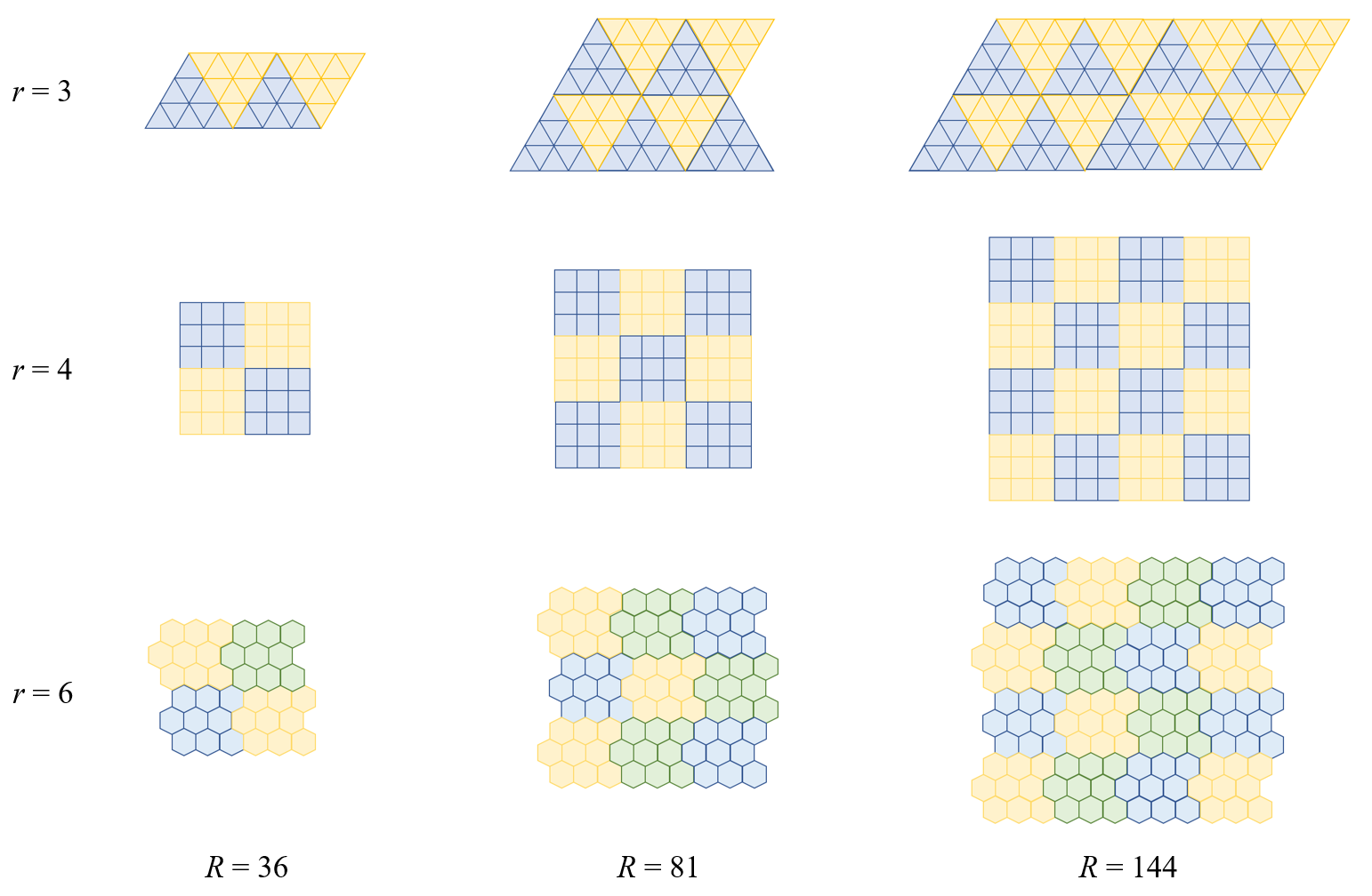
Figure 3: Simulation layout showcasing regional patterns. Each row illustrates configurations with a maximum number of neighbors per region, specifically $r=$3, 4, and 6. The columns indicate varying total counts of regions, with $R=$36, 81, and 144. Within each panel, distinct colors denote separate clusters, leading to varying cluster counts of $m=$4, 9, and 16.

Tables 1 and 2 present the empirical values of $r_{1}={\operatorname{MSE}}(\widehat{\tau}^{i})/{\operatorname{MSE}}(\widehat{\tau}^{g})$ and $r_{2}={\operatorname{MSE}}(\widehat{\tau}^{c})/{\operatorname{MSE}}(\widehat{\tau}^{g})$, showcasing the MSE ratios with and without the presence of interference, respectively. These values are observed under the noise covariance structures outlined in Examples 1 to 3. It’s important to note that a higher $\rho$ value indicates a stronger correlation among the noise across different regions. To explore the effects of this correlation strength on the potential benefits, we conducted simulations with $\rho$ values set at 0.9, 0.6, and 0.3. The theoretical upper bounds shown in brackets were calculated in accordance with Corollary 2. Regarding the structure of interference, we consider a region $\iota$ to have interference from neighboring regions if it shares a single edge with those regions.

We have several important findings. Firstly, the spatially randomized designs generally yield lower MSEs compared to the global design, suggesting that spatial randomization can effectively diminish estimation errors. This advantage of spatially randomized designs becomes even more pronounced as the noise correlation $\rho$ and/or the total number of regions $R$ increase. Secondly, in scenarios where interference is present, the individual-randomized design tends to be more effective than the cluster-randomized design, particularly when the number of sides per region $r$ is low (e.g., $r=3,4$). However, for larger values of $r$ (e.g., $r=6$), the cluster-randomized design proves to be more efficient. Lastly, in the absence of interference, the individual-randomized design is generally the preferred option. These findings lend empirical support to the theoretical propositions outlined in Corollaries 2 and 3.

Table 1: Empirical values of $r_{1}={\operatorname{MSE}}(\widehat{\tau}^{i})/{\operatorname{MSE}}(\widehat{\tau}^{g})$ and $r_{2}={\operatorname{MSE}}(\widehat{\tau}^{c})/{\operatorname{MSE}}(\widehat{\tau}^{g})$ in the parametric regression of nondynamic stage with interference.

			Example 1			Example 2			Example 3
$r$	$\rho$	ratio	$R=36$	$R=64$	$R=144$	$R=36$	$R=64$	$R=144$	$R=36$	$R=64$	$R=144$
3	0.9	$r_{1}$	0.366	0.211	0.121	0.360	0.214	0.117	0.420	0.226	0.142
		$r_{2}$	0.525	0.367	0.188	0.522	0.370	0.185	0.572	0.396	0.210
	0.6	$r_{1}$	0.417	0.204	0.151	0.379	0.200	0.134	0.693	0.356	0.238
		$r_{2}$	0.569	0.347	0.203	0.554	0.361	0.196	0.817	0.531	0.294
	0.3	$r_{1}$	0.556	0.244	0.208	0.421	0.195	0.155	1.454	0.846	0.625
		$r_{2}$	0.626	0.340	0.222	0.593	0.361	0.212	1.101	0.873	0.588
4	0.9	$r_{1}$	0.552	0.308	0.191	0.544	0.316	0.187	0.658	0.321	0.227
		$r_{2}$	0.641	0.456	0.250	0.641	0.457	0.246	0.723	0.469	0.286
	0.6	$r_{1}$	0.623	0.300	0.232	0.582	0.306	0.219	1.015	0.501	0.374
		$r_{2}$	0.694	0.444	0.273	0.690	0.460	0.272	0.956	0.663	0.406
	0.3	$r_{1}$	0.815	0.365	0.302	0.661	0.319	0.259	2.167	1.191	0.883
		$r_{2}$	0.762	0.454	0.300	0.759	0.485	0.309	1.306	0.984	0.64
6	0.9	$r_{1}$	1.006	0.562	0.358	0.982	0.577	0.357	1.182	0.585	0.415
		$r_{2}$	0.675	0.491	0.274	0.674	0.493	0.271	0.762	0.510	0.316
	0.6	$r_{1}$	1.120	0.530	0.413	1.042	0.557	0.413	1.779	0.881	0.653
		$r_{2}$	0.729	0.478	0.300	0.724	0.497	0.298	0.98	0.708	0.448
	0.3	$r_{1}$	1.395	0.594	0.499	1.171	0.577	0.485	3.512	1.877	1.339
		$r_{2}$	0.801	0.488	0.326	0.795	0.524	0.339	1.308	1.014	0.667

Table 2: Empirical values of $r_{1}={\operatorname{MSE}}(\widehat{\tau}^{i})/{\operatorname{MSE}}(\widehat{\tau}^{g})$ and $r_{2}={\operatorname{MSE}}(\widehat{\tau}^{c})/{\operatorname{MSE}}(\widehat{\tau}^{g})$ in the parametric regression of nondynamic stage without interference.

			Example 1			Example 2			Example 3
$r$	$\rho$	ratio	$R=36$	$R=64$	$R=144$	$R=36$	$R=64$	$R=144$	$R=36$	$R=64$	$R=144$
3	0.9	$r_{1}$	0.031	0.016	0.009	0.028	0.015	0.008	0.045	0.020	0.013
		$r_{2}$	0.229	0.128	0.062	0.229	0.129	0.061	0.259	0.140	0.073
	0.6	$r_{1}$	0.049	0.020	0.014	0.032	0.015	0.010	0.100	0.043	0.026
		$r_{2}$	0.254	0.126	0.070	0.253	0.132	0.068	0.408	0.215	0.117
	0.3	$r_{1}$	0.097	0.038	0.028	0.040	0.016	0.012	0.340	0.156	0.098
		$r_{2}$	0.295	0.132	0.082	0.288	0.142	0.079	0.826	0.419	0.256
4	0.9	$r_{1}$	0.031	0.016	0.009	0.028	0.015	0.008	0.045	0.020	0.013
		$r_{2}$	0.229	0.128	0.062	0.229	0.129	0.061	0.259	0.140	0.073
	0.6	$r_{1}$	0.049	0.020	0.014	0.032	0.015	0.010	0.100	0.043	0.026
		$r_{2}$	0.254	0.126	0.070	0.253	0.132	0.068	0.408	0.215	0.117
	0.3	$r_{1}$	0.097	0.038	0.028	0.040	0.016	0.012	0.340	0.156	0.098
		$r_{2}$	0.295	0.132	0.082	0.288	0.142	0.079	0.826	0.419	0.256
6	0.9	$r_{1}$	0.031	0.016	0.009	0.028	0.015	0.008	0.045	0.020	0.013
		$r_{2}$	0.229	0.128	0.062	0.229	0.129	0.061	0.259	0.140	0.073
	0.6	$r_{1}$	0.049	0.020	0.014	0.032	0.015	0.010	0.100	0.043	0.026
		$r_{2}$	0.254	0.126	0.070	0.253	0.132	0.068	0.408	0.215	0.117
	0.3	$r_{1}$	0.097	0.038	0.028	0.040	0.016	0.012	0.340	0.156	0.098
		$r_{2}$	0.295	0.132	0.082	0.288	0.142	0.079	0.826	0.419	0.256

In addition to our main analysis, we explored the inference outcomes using the scenarios presented in Tables 1 and 2. To keep our discussion concise, we’ve chosen to highlight the power curves from Example 2 and have placed the findings from Examples 1 and 3 in the supplementary material. We compare scenarios with and without interference, as illustrated in Figure 4. When the null hypothesis is true (i.e., $s=0$), both designs maintain a rejection probability close to the nominal level of 0.05 across all settings. As the treatment effect size increases, so does the test power. The power curves for the classical global design remain relatively consistent, irrespective of the presence of interference. However, the spatially randomized designs exhibit significantly higher power in the absence of interference, particularly for the individual randomized design. Overall, spatially randomized designs tend to outperform the classical global design in terms of power, under both scenarios. Furthermore, Figure 4 shows that the power of spatially randomized designs improves notably with either an increase in the number of regions $R$ or a reduction in the number of neighboring sides, especially when interference is accounted for. Conversely, the performance of the classical global design appears largely unaffected by these factors.

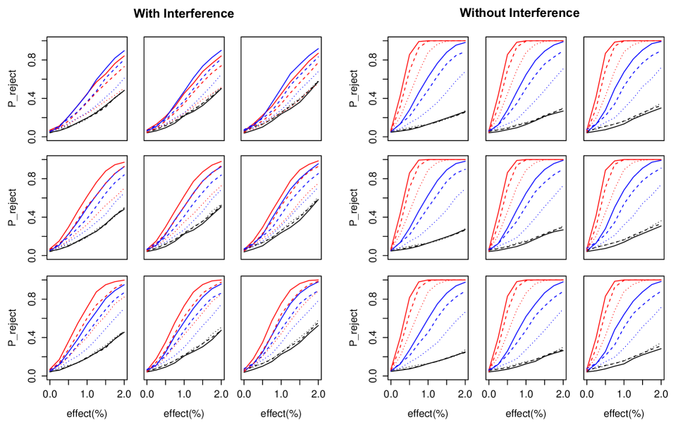
Figure 4: Rejection probabilities in the parametric regression model under a non-dynamic setup, considering both scenarios with and without interference. These probabilities are presented for cases where the noise follows the covariance structure from Example 2, with the treatment’s relative efficacy varying from $0\%$ to $2.0\%$. The red lines depict the individual-randomized design, while the blue lines represent the cluster-randomized design, and the black lines denote the global randomized design. The line styles-solid, dashed, and dotted-correspond to the number of regions $R=144,81,$ and $36,$ respectively. The figure is organized into three rows and three columns of panels, representing different values of $r$ (6, 4, and 3) and $\rho$ (0.9, 0.6, and 0.3), respectively.

For the nonparametric model of nondynamic setting, the underlying model is

$$Y_{t,\iota}=5+3(O_{t,\iota}+\overline{O}_{i\iota})\sin\left\{\frac{\pi}{8}(\iota_{x}+\iota_{y})+s\cdot A_{t,\iota}+0.5\cdot s\cdot\overline{A}_{t,\iota}\right\}+0.5e_{i\iota},$$

where the covariates $O_{t,\iota}$ are independently drawn from a truncated Gaussian distribution $N(4,1)$ within the range $(3,5)$, and the noise terms $e_{i\iota}$ have zero mean with a covariance structure as described in Examples 1 to 3. The treatment effects $s$ are simulated at levels $0,0.0025,0.005,0.0075,0.01,0.0125,0.015$, corresponding to improvements of $0\%,0.25\%,0.5\%,0.75\%,1\%,1.25\%,1.5\%$ over the control outcome. The other parameters follow the same settings as in the parametric models. We vary the correlation strength $\rho$ at $0.3,0.6,0.9$, and the total number of regions $R$ at $36,64,144$, with $N=30$ observations per region, configuring the regions as equilateral triangles, squares, and hexagons for $r=3,4,6$, respectively, as illustrated in Figure 3.

Tables 3 and 4 display the empirical ratios $r_{1}={\operatorname{MSE}}(\widehat{\tau}_{DR}^{i})/{\operatorname{MSE}}(\widehat{\tau}_{DR}^{g})$ and $r_{2}={\operatorname{MSE}}(\widehat{\tau}_{DR}^{c})/{\operatorname{MSE}}(\widehat{\tau}_{DR}^{g})$, while Figure 5 showcases the power curves under different configurations. Our results indicate that the spatially randomized designs yield more efficient estimation and inference than the traditional global design in a static framework. The advantages of spatial randomization become more evident with an increase in the number of regions $R$ and/or a decrease in the number of neighbors $r$. Additionally, the impact of the number of neighbors $r$ appears to be more pronounced on $\widehat{\tau}_{DR}^{i}$ compared to $\widehat{\tau}_{DR}^{c}$, aligning with the insights from Corollary 3.

Table 3: Empirical values of $r_{1}={\operatorname{MSE}}(\widehat{\tau}_{DR}^{i})/{\operatorname{MSE}}(\widehat{\tau}_{DR}^{g})$ and $r_{2}={\operatorname{MSE}}(\widehat{\tau}_{DR}^{c})/{\operatorname{MSE}}(\widehat{\tau}_{DR}^{g})$ in the nonparametric regression of nondynamic stage with interference.

			Example 1			Example 2			Example 3
$r$	$\rho$	ratio	$R=36$	$R=64$	$R=144$	$R=36$	$R=64$	$R=144$	$R=36$	$R=64$	$R=144$
3	0.9	$r_{1}$	0.188	0.103	0.065	0.186	0.103	0.062	0.223	0.125	0.078
		$r_{2}$	0.315	0.156	0.092	0.306	0.163	0.089	0.359	0.170	0.108
	0.6	$r_{1}$	0.236	0.116	0.079	0.202	0.106	0.068	0.403	0.212	0.138
		$r_{2}$	0.363	0.160	0.101	0.331	0.173	0.095	0.533	0.258	0.160
	0.3	$r_{1}$	0.379	0.175	0.111	0.239	0.118	0.079	0.975	0.550	0.357
		$r_{2}$	0.448	0.189	0.119	0.378	0.192	0.107	0.874	0.479	0.343
4	0.9	$r_{1}$	0.362	0.170	0.100	0.352	0.165	0.096	0.482	0.214	0.123
		$r_{2}$	0.452	0.192	0.105	0.438	0.199	0.102	0.548	0.212	0.122
	0.6	$r_{1}$	0.465	0.204	0.122	0.382	0.175	0.107	0.854	0.373	0.212
		$r_{2}$	0.564	0.204	0.116	0.484	0.214	0.111	0.881	0.339	0.184
	0.3	$r_{1}$	0.799	0.316	0.172	0.459	0.204	0.127	2.212	0.898	0.539
		$r_{2}$	0.843	0.259	0.139	0.576	0.244	0.129	2.052	0.717	0.393
6	0.9	$r_{1}$	0.297	0.141	0.083	0.286	0.138	0.080	0.380	0.174	0.103
		$r_{2}$	0.373	0.182	0.105	0.363	0.190	0.102	0.435	0.198	0.121
	0.6	$r_{1}$	0.381	0.172	0.101	0.316	0.153	0.090	0.682	0.290	0.181
		$r_{2}$	0.440	0.188	0.115	0.399	0.203	0.111	0.627	0.303	0.179
	0.3	$r_{1}$	0.625	0.265	0.141	0.385	0.185	0.107	1.714	0.742	0.493
		$r_{2}$	0.579	0.225	0.135	0.466	0.231	0.129	1.166	0.598	0.373

Table 4: Empirical values of $r_{1}={\operatorname{MSE}}(\widehat{\tau}_{DR}^{i})/{\operatorname{MSE}}(\widehat{\tau}_{DR}^{g})$ and $r_{2}={\operatorname{MSE}}(\widehat{\tau}_{DR}^{c})/{\operatorname{MSE}}(\widehat{\tau}_{DR}^{g})$ in the nonparametric regression of nondynamic stage without interference.

			Example 1			Example 2			Example 3
$r$	$\rho$	ratio	$R=36$	$R=64$	$R=144$	$R=36$	$R=64$	$R=144$	$R=36$	$R=64$	$R=144$
3	0.9	$r_{1}$	0.028	0.013	0.008	0.026	0.012	0.008	0.040	0.017	0.011
		$r_{2}$	0.126	0.072	0.044	0.122	0.075	0.042	0.244	0.107	0.064
	0.6	$r_{1}$	0.044	0.018	0.012	0.030	0.013	0.009	0.089	0.036	0.022
		$r_{2}$	0.148	0.077	0.049	0.132	0.080	0.045	0.384	0.171	0.102
	0.3	$r_{1}$	0.093	0.037	0.023	0.038	0.016	0.010	0.290	0.126	0.077
		$r_{2}$	0.188	0.097	0.060	0.150	0.089	0.050	0.789	0.350	0.240
4	0.9	$r_{1}$	0.035	0.014	0.008	0.033	0.013	0.008	0.051	0.019	0.011
		$r_{2}$	0.288	0.114	0.061	0.276	0.116	0.059	0.334	0.119	0.064
	0.6	$r_{1}$	0.054	0.020	0.012	0.037	0.014	0.009	0.113	0.040	0.023
		$r_{2}$	0.390	0.128	0.069	0.310	0.124	0.064	0.581	0.199	0.104
	0.3	$r_{1}$	0.113	0.040	0.023	0.047	0.017	0.010	0.359	0.136	0.081
		$r_{2}$	0.675	0.183	0.092	0.378	0.141	0.074	1.477	0.445	0.251
6	0.9	$r_{1}$	0.029	0.013	0.008	0.027	0.013	0.008	0.041	0.018	0.011
		$r_{2}$	0.203	0.100	0.054	0.198	0.104	0.052	0.265	0.110	0.063
	0.6	$r_{1}$	0.045	0.018	0.012	0.031	0.013	0.008	0.091	0.038	0.022
		$r_{2}$	0.251	0.104	0.061	0.219	0.112	0.058	0.426	0.178	0.100
	0.3	$r_{1}$	0.094	0.038	0.023	0.039	0.016	0.010	0.293	0.128	0.078
		$r_{2}$	0.368	0.129	0.076	0.259	0.127	0.068	0.945	0.375	0.237

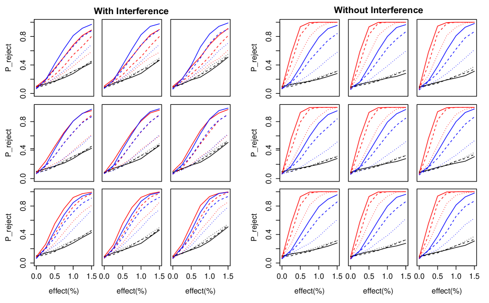
Figure 5: Rejection probability in the nonparametric regression of nondynamic setting under different relative improvements of the new policy. The red, blue and black lines represent to the individual-, cluster and global-randomized designs, with $R=144,81,36$ in solid, dashed and dotted lines, respectively. The three rows of panels correspond to $r=6,4,3$, and the three columns correspond to $\rho=0.9,0.6,0.3$, respectively.

4.2 Simulation of the dynamic setting

In the dynamic parametric model, we maintain the same regional configurations as in the static cases and initiate the covariates $O_{i\iota 1}$ as independent and identically distributed normal variables $N(4,1)$. For subsequent times $t\geq 1$, the covariates $O_{i\iota t}$ are generated based on the specified model (14). The coefficients $\alpha_{\iota t},\beta_{\iota t}$, and $\Lambda_{\iota t}$ are defined as follows, incorporating temporal variation through functions $h_{1}(t),h_{2}(t),$ and $h_{3}(t)$, respectively:

$$\alpha_{\iota t}=h_{1}(t)\{8+2(f_{1}(\iota_{x})+g_{1}(\iota_{y}))\},\ \beta_{\iota t}=h_{2}(t)\{f_{2}(\iota_{x})+g_{2}(\iota_{y})\},\ \Lambda_{\iota t}=h_{3}(t)\{f_{3}(\iota_{x})+g_{3}(\iota_{y})\},$$

where each $h_{i}(t)$ takes the form $a_{0}+\sum_{k=1}^{K}{a_{k}\cos(k\pi x)+b_{k}\sin(k\pi x)}$, with coefficients $a_{0},a_{k},b_{k}$ randomly drawn from a uniform distribution over $[0,1]$ and $K=3$. The coefficients $B_{\iota t}$ are constructed as:

$$B_{\iota t}^{0}=h_{4}(t)\{f_{4}(\iota_{x})+g_{4}(\iota_{y})\},\quad B_{\iota t}=\frac{1}{2}\cdot\frac{B_{\iota t}^{0}-\min_{\iota,t}B_{\iota t}^{0}}{\max_{\iota,t}B_{\iota t}^{0}-\min_{\iota,t}B_{\iota t}^{0}}+0.3.$$

We consider Gaussian noises $e_{i\iota t}$ which are i.i.d copies with $e_{\iota}$ in Example 2 and state noises $E_{i\iota t}$ are i.i.d copies of $0.3e_{\iota}$. The effect coefficients $\gamma_{\iota t},\theta_{\iota t},\Gamma_{\iota t},$ and $\Theta_{\iota t}$ are generated in alignment with the patterns of $\alpha_{\iota t},\beta_{\iota t},\Lambda_{\iota t},$ and $B_{\iota t}$, scaled by the aggregate signal strengths $s_{x}$ and $s_{y}$:

$$\gamma_{\iota t}=s_{y}\cdot\frac{\alpha_{\iota t}}{\sum_{\iota}\sum_{t}\alpha_{\iota t}},\quad\theta_{\iota t}=s_{y}\cdot\frac{3}{5}\cdot\frac{\beta_{\iota t}}{\sum_{\iota}\sum_{t}\beta_{\iota t}},$$

$$\Gamma_{\iota t}=s_{x}\cdot\frac{\Lambda_{\iota t}}{\sum_{\iota}\sum_{t}\Lambda_{\iota t}},\quad\Theta_{\iota t}=s_{x}\cdot\frac{3}{5}\cdot\frac{B_{\iota t}}{\sum_{\iota}\sum_{t}B_{\iota t}},$$

where $s_{x}$ and $s_{y}$ are the signal strengths generated as follows,

$$s_{x}=s\cdot\sum_{\iota}\sum_{t}{\mathbb{E}}(O_{\iota t}|A_{jk}=0,1\leq j\leq R,1\leq k\leq M),$$

$$s_{y}=s\cdot\sum_{\iota}\sum_{t}{\mathbb{E}}(Y_{\iota t}|A_{jk}=0,1\leq j\leq R,1\leq k\leq M),$$

which corresponds to $100s\%$ improvement. The simulations are conducted across a range of configurations, including $r=3,4,6$ for the number of neighbors, $\rho=0.3,0.6,0.9$ for the noise correlation, $R=36,81,144$ for the total number of regions, and $M=12$ time intervals, with each region having $N=30$ observations.

For the nonparametric model, the underlying model is

$$Y_{i\iota t}=5+2\cdot O_{i\iota t}\sin\left\{\frac{\pi}{8}(\iota_{x}+\iota_{y}+t/M)+s\cdot(A_{i\iota t}+\overline{A}_{i\iota t})\right\}+0.5e_{i\iota t},$$

where $(O_{i1t},\ldots,O_{iRt})^{\top}$ are i.i.d multivariate Gaussian with mean $(2+A_{i1t},\ldots,2+A_{iRt})^{\top}$ and covariance taking the form in Example 3 of $\rho=0.3,0.6,0.9$. Other parameters are set the same as the parametric case. We simulate $r=3,4,6$, $R=36,81,144$ and $M=12$ with $N=40$.

Table 5 showcases the empirical ratios $r_{1}={\operatorname{MSE}}(\widehat{\tau}_{OLS}^{i})/{\operatorname{MSE}}(\widehat{\tau}_{OLS}^{g})$ and $r_{2}={\operatorname{MSE}}(\widehat{\tau}_{OLS}^{c})/{\operatorname{MSE}}(\widehat{\tau}_{OLS}^{g})$ across various scenarios. The findings indicate that the relationships between these ratios and the parameters $\rho$, $R$, and $r$ align with those observed in the static, single-stage setting, thereby corroborating the assertions of Theorems 4 and 5. We conducted experiments with diverse levels of $s$ for both parametric and nonparametric models and depicted the resulting power curves in Figure 6. In each instance, spatially randomized designs demonstrate superior performance over the conventional global design in terms of power, underscoring the benefits of spatial randomization in dynamic settings.

Table 5: Empirical values of $r_{1}={\operatorname{MSE}}(\widehat{\tau}_{M}^{i})/{\operatorname{MSE}}(\widehat{\tau}_{M}^{g})$ and $r_{2}={\operatorname{MSE}}(\widehat{\tau}_{M}^{c})/{\operatorname{MSE}}(\widehat{\tau}_{M}^{g})$ in the parametric and nonparametric regressions of dynamic setting with interference when the noises are generated according to Example 2.

			parametric			nonparametric
$r$	$\rho$	ratio	$R=36$	$R=64$	$R=144$	$R=36$	$R=64$	$R=144$
3	0.9	$r_{1}$	0.315	0.249	0.116	0.139	0.073	0.033
		$r_{2}$	0.495	0.291	0.103	0.641	0.425	0.224
	0.6	$r_{1}$	0.350	0.252	0.126	0.135	0.070	0.032
		$r_{2}$	0.513	0.302	0.114	0.713	0.474	0.250
	0.3	$r_{1}$	0.410	0.267	0.142	0.152	0.075	0.033
		$r_{2}$	0.543	0.326	0.138	0.809	0.587	0.296
4	0.9	$r_{1}$	0.551	0.434	0.196	0.181	0.084	0.037
		$r_{2}$	0.693	0.388	0.158	0.666	0.355	0.218
	0.6	$r_{1}$	0.603	0.444	0.211	0.156	0.082	0.035
		$r_{2}$	0.738	0.416	0.179	0.757	0.409	0.245
	0.3	$r_{1}$	0.694	0.475	0.238	0.181	0.085	0.038
		$r_{2}$	0.808	0.471	0.224	0.871	0.503	0.291
6	0.9	$r_{1}$	1.067	0.709	0.366	0.193	0.089	0.043
		$r_{2}$	0.726	0.428	0.165	0.705	0.352	0.221
	0.6	$r_{1}$	1.158	0.727	0.395	0.162	0.088	0.041
		$r_{2}$	0.773	0.457	0.189	0.790	0.410	0.249
	0.3	$r_{1}$	1.310	0.778	0.445	0.187	0.092	0.044
		$r_{2}$	0.844	0.515	0.237	0.919	0.502	0.295

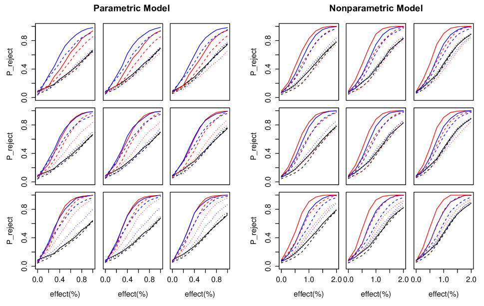
Figure 6: Rejection probability in the parametric and nonparametric models with $M=12$ of multi-stage case under different relative improvements of the new policy. The red, blue and black lines represent to the individual-, cluster and global-randomized designs, with $R=144,81,36$ plotted in solid, dashed and dotted lines, respectively. The three rows of panels correspond to $r=6,4,3$, and the three columns correspond to $\rho=0.9,0.6,0.3$, respectively.

4.3 Real data based simulation

In this section, we evaluate the efficacy of our proposed experimental framework by simulating a real online ride-hailing service, using the same simulator referenced in Zhou et al. (2021). This simulator accurately models the dynamic interplay between demand and supply, mirroring an actual ride-hailing platform. It generates demand distributions from historical data, while initial driver supply distributions are based on early-day data, subsequently adjusted through the simulator’s dynamic transitions and order dispatch algorithms. The simulation’s key metrics, such as driver earnings, response rates, and idle times, deviate from real-world figures by less than 2%.

For our analysis, we selected the largest square region of the city, dividing it into $64$ equally sized, non-overlapping squares ($R=64$). Over $N=20$ days, segmented into $M=24$ hourly intervals, we investigated the effects of policies simulating ATE improvements of $0\%,1.0\%,2\%$, and $5\%$. We applied a parametric regression model for the multi-stage scenario to estimate and analyze the ATE, comparing the classical global design with an individual randomized design that incorporates temporal randomization. The outcomes of these designs are denoted by $\widehat{\tau}^{i}_{OLS}$ and $\widehat{\tau}^{g}_{OLS}$, respectively.

Using 300 Monte Carlo simulations to closely estimate the true ATE, we compiled the test powers and MSE ratios ${\operatorname{MSE}}(\widehat{\tau}^{i}_{OLS})/{\operatorname{MSE}}(\widehat{\tau}^{g}_{OLS})$ in Table 6. Our findings indicate that both the classical global and spatially randomized designs maintain proper type I error rates. Notably, the spatially randomized design consistently exhibited lower MSE and higher test power compared to the classical global approach, irrespective of interference effects. This evidence strongly supports the superior efficiency of the spatially randomized design in real-world applications.

Table 6: The test powers and MSE ratios ${\operatorname{MSE}}(\widehat{\tau}_{OLS}^{i})/{\operatorname{MSE}}(\widehat{\tau}_{OLS}^{g})$ of the data produced by the Simulator.

		ATE-test		MSE ratio
		benchmark	proposed
0%	no-interference	0.07	0.06	0.010
	interference-existing		0.05	0.129
1.0%	no-interference	0.16	1.00	0.013
	interference-existing		0.32	0.134
2%	no-interference	0.33	1.00	0.016
	interference-existing		0.89	0.128
5%	no-interference	0.87	1.00	0.037
	interference-existing		1.00	0.158

5 Discussion

In this paper, we aim at enhancing the precision of ATE estimation and the efficiency of inference across various scenarios by distributing treatment randomly among regions. A pivotal discovery of our research is that randomization effectively diminishes the spatial correlation of noise. Under standard conditions, we observe that the MSE ratio of ATE estimators, derived from spatially randomized designs compared to conventional global designs, is inversely related to the count of regions or clusters, applicable in both static and dynamic frameworks. Additionally, we advocate for the application of smoothing techniques on OLS coefficient estimators as a means to lower MSE, although this does not enhance the order of convergence of the outcomes and thus is omitted from the main discussion. Further details on this method are available in the supplementary materials.

Moving forward, there are several important topics worthy of further investigation. Firstly, examining experimental designs when temporal random effects are present is an interesting issue. Temporal random effects in the residual may cause endogeneity bias in the autoregressive coefficient of the state regression model, resulting in inconsistent ATE estimation. To tackle this inconsistency, one approach is to use historical data in which actions were set to baseline policies to estimate autoregressive coefficients. Another solution is to assume that random effects satisfy certain covariance structures such as declining correlation as temporal distance increases. Secondly, we have focused on the inference properties of multi-stages with finite time frames. However, for infinite stages, where a variance estimate is likely to become infinite, Gaussian approximation techniques may be applied to overcome the problem, as discussed in Luo et al. (2024). Finally, we considered a general and simplistic interference structure in this study. Investigating interference structures that are more complex across space would be an interesting problem.

References

- Aronow and Samii (2017) Aronow, P. M. and C. Samii (2017). Estimating average causal effects under general interference, with application to a social network experiment. The Annals of Applied Statistics 11(4), 1912–1947.
- Baird et al. (2018) Baird, S., J. A. Bohren, C. McIntosh, and B. Özler (2018). Optimal design of experiments in the presence of interference. Review of Economics and Statistics 100(5), 844–860.
- Bajari et al. (2021) Bajari, P., B. Burdick, G. W. Imbens, L. Masoero, J. McQueen, T. Richardson, and I. M. Rosen (2021). Multiple randomization designs. arXiv preprint arXiv:2112.13495.
- Basse and Airoldi (2018) Basse, G. W. and E. M. Airoldi (2018). Model-assisted design of experiments in the presence of network-correlated outcomes. Biometrika 105(4), 849–858.
- Bergsma (2004) Bergsma, W. P. (2004). Testing conditional independence for continuous random variables.
- Bojinov et al. (2023) Bojinov, I., D. Simchi-Levi, and J. Zhao (2023). Design and analysis of switchback experiments. Management Science 69(7), 3759–3777.
- Chen and Hong (2012) Chen, B. and Y. Hong (2012). Testing for the markov property in time series. Econometric Theory 28(1), 130–178.
- Chernozhukov et al. (2018) Chernozhukov, V., D. Chetverikov, M. Demirer, E. Duflo, C. Hansen, W. Newey, and J. Robins (2018). Double/debiased machine learning for treatment and structural parameters. The Econometrics Journal 21(1).
- Díaz (2020) Díaz, I. (2020). Machine learning in the estimation of causal effects: targeted minimum loss-based estimation and double/debiased machine learning. Biostatistics 21(2), 353–358.
- Halloran and Struchiner (1991) Halloran, M. E. and C. J. Struchiner (1991). Study designs for dependent happenings. Epidemiology, 331–338.
- Halloran and Struchiner (1995) Halloran, M. E. and C. J. Struchiner (1995). Causal inference in infectious diseases. Epidemiology, 142–151.
- Hu and Hu (2012) Hu, Y. and F. Hu (2012). Asymptotic properties of covariate-adaptive randomization. The Annals of Statistics 40(3), 1794–1815.
- Hu and Wager (2022) Hu, Y. and S. Wager (2022). Switchback experiments under geometric mixing. arXiv preprint arXiv:2209.00197.
- Hudgens and Halloran (2008) Hudgens, M. G. and M. E. Halloran (2008). Toward causal inference with interference. Journal of the American Statistical Association 103(482), 832–842.
- Imbens and Rubin (2015) Imbens, G. W. and D. B. Rubin (2015). Causal inference in statistics, social, and biomedical sciences. Cambridge University Press.
- Jagadeesan et al. (2020) Jagadeesan, R., N. S. Pillai, and A. Volfovsky (2020). Designs for estimating the treatment effect in networks with interference. The Annals of Statistics 48(2), 679–712.
- Jiang and Li (2016) Jiang, N. and L. Li (2016). Doubly robust off-policy value evaluation for reinforcement learning. In International Conference on Machine Learning, pp. 652–661. PMLR.
- Johari et al. (2022) Johari, R., H. Li, I. Liskovich, and G. Y. Weintraub (2022). Experimental design in two-sided platforms: An analysis of bias. Management Science 68(10), 7069–7089.
- Kalish and Begg (1985) Kalish, L. A. and C. B. Begg (1985). Treatment allocation methods in clinical trials: a review. Statistics in medicine 4(2), 129–144.
- Kallus and Uehara (2020) Kallus, N. and M. Uehara (2020). Double reinforcement learning for efficient off-policy evaluation in markov decision processes. Journal of Machine Learning Research 21(167), 6742–6804.
- Kallus and Uehara (2022) Kallus, N. and M. Uehara (2022). Efficiently breaking the curse of horizon in off-policy evaluation with double reinforcement learning. Operations Research 70(6), 3282–3302.
- Ke et al. (2018) Ke, J., H. Yang, H. Zheng, X. Chen, Y. Jia, P. Gong, and J. Ye (2018). Hexagon-based convolutional neural network for supply-demand forecasting of ride-sourcing services. IEEE Transactions on Intelligent Transportation Systems 20(11), 4160–4173.
- Kong et al. (2021) Kong, X., M. Yuan, and W. Zheng (2021). Approximate and exact designs for total effects. The Annals of Statistics 49(3), 1594–1625.
- Larsen et al. (2022) Larsen, A., S. Yang, B. J. Reich, and A. G. Rappold (2022). A spatial causal analysis of wildland fire-contributed pm2. 5 using numerical model output. The Annals of Applied Statistics 16(4), 2714–2731.
- Leung (2022) Leung, M. P. (2022). Rate-optimal cluster-randomized designs for spatial interference. The Annals of Statistics 50(5), 3064–3087.
- Li et al. (2023) Li, T., C. Shi, J. Wang, F. Zhou, et al. (2023). Optimal treatment allocation for efficient policy evaluation in sequential decision making. Advances in Neural Information Processing Systems 36.
- Li et al. (2019) Li, X., P. Ding, Q. Lin, D. Yang, and J. S. Liu (2019). Randomization inference for peer effects. Journal of the American Statistical Association 114(528), 1651–1664.
- Liao et al. (2021) Liao, P., P. Klasnja, and S. Murphy (2021). Off-policy estimation of long-term average outcomes with applications to mobile health. Journal of the American Statistical Association 116(533), 382–391.
- Liao et al. (2022) Liao, P., Z. Qi, R. Wan, P. Klasnja, and S. A. Murphy (2022). Batch policy learning in average reward markov decision processes. The Annals of Statistics 50(6), 3364–3387.
- Liu et al. (2016) Liu, L., M. G. Hudgens, and S. Becker-Dreps (2016). On inverse probability-weighted estimators in the presence of interference. Biometrika 103(4), 829–842.
- Liu et al. (2018) Liu, Q., L. Li, Z. Tang, and D. Zhou (2018). Breaking the curse of horizon: Infinite-horizon off-policy estimation. Advances in Neural Information Processing Systems 31.
- Luckett et al. (2019) Luckett, D. J., E. B. Laber, A. R. Kahkoska, D. M. Maahs, E. Mayer-Davis, and M. R. Kosorok (2019). Estimating dynamic treatment regimes in mobile health using v-learning. Journal of the American Statistical Association.
- Luedtke and Van Der Laan (2016) Luedtke, A. R. and M. J. Van Der Laan (2016). Statistical inference for the mean outcome under a possibly non-unique optimal treatment strategy. Annals of statistics 44(2), 713.
- Luo et al. (2024) Luo, S., Y. Yang, C. Shi, F. Yao, J. Ye, and H. Zhu (2024). Policy evaluation for temporal and/or spatial dependent experiments. Journal of the Royal Statistical Society, Series B, in press.
- Munro et al. (2021) Munro, E., S. Wager, and K. Xu (2021). Treatment effects in market equilibrium. arXiv preprint arXiv:2109.11647.
- Murphy (2003) Murphy, S. A. (2003). Optimal dynamic treatment regimes. Journal of the Royal Statistical Society Series B: Statistical Methodology 65(2), 331–355.
- Perez-Heydrich et al. (2014) Perez-Heydrich, C., M. G. Hudgens, M. E. Halloran, J. D. Clemens, M. Ali, and M. E. Emch (2014, September). Assessing effects of cholera vaccination in the presence of interference. Biometrics 70(3), 731–741.
- Pocock and Simon (1975) Pocock, S. J. and R. Simon (1975). Sequential treatment assignment with balancing for prognostic factors in the controlled clinical trial. Biometrics 31(1), 103–115.
- Puelz et al. (2022) Puelz, D., G. Basse, A. Feller, and P. Toulis (2022). A graph-theoretic approach to randomization tests of causal effects under general interference. Journal of the Royal Statistical Society Series B: Statistical Methodology 84(1), 174–204.
- Puterman (2014) Puterman, M. L. (2014). Markov decision processes: discrete stochastic dynamic programming. John Wiley & Sons.
- Reich et al. (2021) Reich, B. J., S. Yang, Y. Guan, A. B. Giffin, M. J. Miller, and A. Rappold (2021). A review of spatial causal inference methods for environmental and epidemiological applications. International Statistical Review 89(3), 605–634.
- Robins et al. (2000) Robins, J. M., M. A. Hernan, and B. Brumback (2000). Marginal structural models and causal inference in epidemiology. Epidemiology, 550–560.
- Rosenberger and Sverdlov (2008) Rosenberger, W. F. and O. Sverdlov (2008). Handling covariates in the design of clinical trials. Statistical Science, 404–419.
- Rysman (2009) Rysman, M. (2009). The economics of two-sided markets. Journal of Economic Perspectives 23(3), 125–143.
- Shah and Peters (2020) Shah, R. D. and J. Peters (2020). The hardness of conditional independence testing and the generalised covariance measure. The Annals of Statistics 48(3), 1514–1538.
- Shi et al. (2021) Shi, C., R. Song, and W. Lu (2021). Concordance and value information criteria for optimal treatment decision. Annals of Statistics 49(1), 49–75.
- Shi et al. (2021) Shi, C., R. Wan, V. Chernozhukov, and R. Song (2021). Deeply-debiased off-policy interval estimation. In International Conference on Machine Learning, pp. 9580–9591. PMLR.
- Shi et al. (2022) Shi, C., R. Wan, G. Song, S. Luo, R. Song, and H. Zhu (2022). A multi-agent reinforcement learning framework for off-policy evaluation in two-sided markets. arXiv preprint arXiv:2202.10574.
- Shi et al. (2020) Shi, C., R. Wan, R. Song, W. Lu, and L. Leng (2020). Does the markov decision process fit the data: Testing for the markov property in sequential decision making. In International Conference on Machine Learning, pp. 8807–8817. PMLR.
- Shi et al. (2023) Shi, C., X. Wang, S. Luo, H. Zhu, J. Ye, and R. Song (2023). Dynamic causal effects evaluation in a/b testing with a reinforcement learning framework. Journal of the American Statistical Association 118, 2059–2071.
- Shi et al. (2021) Shi, C., T. Xu, W. Bergsma, and L. Li (2021). Double generative adversarial networks for conditional independence testing. The Journal of Machine Learning Research 22(1), 13029–13060.
- Sobel (2006) Sobel, M. E. (2006). What do randomized studies of housing mobility demonstrate? causal inference in the face of interference. Journal of the American Statistical Association 101(476), 1398–1407.
- Tang et al. (2019) Tang, X., Z. Qin, F. Zhang, Z. Wang, Z. Xu, Y. Ma, H. Zhu, and J. Ye (2019). A deep value-network based approach for multi-driver order dispatching. In Proceedings of the 25th ACM SIGKDD international conference on knowledge discovery & data mining, pp. 1780–1790.
- Taves (1974) Taves, D. R. (1974). Minimization: a new method of assigning patients to treatment and control groups. Clinical Pharmacology & Therapeutics 15(5), 443–453.
- Tchetgen et al. (2021) Tchetgen, E. J., I. R. Fulcher, and I. Shpitser (2021). Auto-g-computation of causal effects on a network. Journal of the American Statistical Association 116(534), 833–844.
- Thomas and Brunskill (2016) Thomas, P. and E. Brunskill (2016). Data-efficient off-policy policy evaluation for reinforcement learning. In International Conference on Machine Learning, pp. 2139–2148. PMLR.
- Tsiatis (2006) Tsiatis, A. A. (2006). Semiparametric theory and missing data. Springer.
- Uehara et al. (2020) Uehara, M., J. Huang, and N. Jiang (2020). Minimax weight and q-function learning for off-policy evaluation. In International Conference on Machine Learning, pp. 9659–9668. PMLR.
- Uehara et al. (2022) Uehara, M., C. Shi, and N. Kallus (2022). A review of off-policy evaluation in reinforcement learning. arXiv preprint arXiv:2212.06355.
- Ugander et al. (2013) Ugander, J., B. Karrer, L. Backstrom, and J. Kleinberg (2013). Graph cluster randomization: Network exposure to multiple universes. In Proceedings of the 19th ACM SIGKDD international conference on Knowledge discovery and data mining, pp. 329–337.
- Verbitsky-Savitz and Raudenbush (2012) Verbitsky-Savitz, N. and S. W. Raudenbush (2012). Causal inference under interference in spatial settings: A case study evaluating community policing program in chicago. Epidemiologic Methods 1, 107–130.
- Viviano (2020) Viviano, D. (2020). Experimental design under network interference. arXiv preprint arXiv:2003.08421.
- Wager and Xu (2021) Wager, S. and K. Xu (2021). Experimenting in equilibrium. Management Science 67(11), 6694–6715.
- Wang et al. (2023) Wang, J., Z. Qi, and R. K. Wong (2023). Projected state-action balancing weights for offline reinforcement learning. The Annals of Statistics 51(4), 1639–1665.
- Wang et al. (2018) Wang, L., Y. Zhou, R. Song, and B. Sherwood (2018). Quantile-optimal treatment regimes. Journal of the American Statistical Association 113(523), 1243–1254.
- Xiong et al. (2023) Xiong, R., A. Chin, and S. J. Taylor (2023). Data-driven switchback designs: Theoretical tradeoffs and empirical calibration. Available at SSRN.
- Xu et al. (2018) Xu, Z., Z. Li, Q. Guan, D. Zhang, Q. Li, J. Nan, C. Liu, W. Bian, and J. Ye (2018). Large-scale order dispatch in on-demand ride-hailing platforms: A learning and planning approach. In Proceedings of the 24th ACM SIGKDD International Conference on Knowledge Discovery & Data Mining, pp. 905–913.
- Yang et al. (2018) Yang, Y., R. Luo, M. Li, M. Zhou, W. Zhang, and J. Wang (2018). Mean field multi-agent reinforcement learning. In International conference on machine learning, pp. 5571–5580. PMLR.
- Zhang et al. (2012) Zhang, B., A. A. Tsiatis, E. B. Laber, and M. Davidian (2012). A robust method for estimating optimal treatment regimes. Biometrics 68(4), 1010–1018.
- Zhang et al. (2013) Zhang, B., A. A. Tsiatis, E. B. Laber, and M. Davidian (2013). Robust estimation of optimal dynamic treatment regimes for sequential treatment decisions. Biometrika 100(3), 681–694.
- Zhang et al. (2011) Zhang, K., J. Peters, D. Janzing, and B. Schölkopf (2011). Kernel-based conditional independence test and application in causal discovery. In Proceedings of the Twenty-Seventh Conference on Uncertainty in Artificial Intelligence, pp. 804–813.
- Zhang et al. (2015) Zhang, Y., E. B. Laber, A. Tsiatis, and M. Davidian (2015). Using decision lists to construct interpretable and parsimonious treatment regimes. Biometrics 71(4), 895–904.
- Zhou et al. (2021) Zhou, F., S. Luo, X. Qie, J. Ye, and H. Zhu (2021). Graph-based equilibrium metrics for dynamic supply–demand systems with applications to ride-sourcing platforms. Journal of the American Statistical Association 116(536), 1688–1699.
- Zhou et al. (2020) Zhou, Y., Y. Liu, P. Li, and F. Hu (2020). Cluster-adaptive network a/b testing: From randomization to estimation. arXiv preprint arXiv:2008.08648.
- Zhou et al. (2023) Zhou, Y., C. Shi, L. Li, and Q. Yao (2023). Testing for the markov property in time series via deep conditional generative learning. arXiv preprint arXiv:2305.19244.
- Zigler et al. (2012) Zigler, C. M., F. Dominici, and Y. Wang (2012). Estimating causal effects of air quality regulations using principal stratification for spatially correlated multivariate intermediate outcomes. Biostatistics 13(2), 289–302.
- Zigler and Papadogeorgou (2021) Zigler, C. M. and G. Papadogeorgou (2021). Bipartite causal inference with interference. Statistical science: a review journal of the Institute of Mathematical Statistics 36(1), 109.