-
March 2024
Determination of a Small Elliptical Anomaly in Electrical Impedance Tomography using Minimal Measurements
Abstract
We consider the problem of determining a small elliptical conductivity anomaly in a unit disc from boundary measurements. The conductivity of the anomaly is assumed to be a small perturbation from the constant background. A measurement of voltage across two point-electrodes on the boundary through which a constant current is passed. We further assume the limiting case when the distance between two electrodes go to zero, creating a dipole field. We show that three such measurements suffice to locate the anomaly size and location inside the disc. Two further measurements are needed to obtain the aspect ratio and the orientation of the ellipse. The investigation includes the studies of the stability of the inverse problem and optimal experiment design.
1 Introduction
This work is motivated by the work of Isakov-Titi [7, 8] which considers the gravimetry inverse problems from minimal measurements. In inverse gravimetry, the goal is to determine the density of a body from gravitational measurements. In their work, the authors break away from classical gravimetry where data are available over a curve or surface. Instead they consider cases where data are available only at a few points. However, instead of reconstructing density distribution, their work focus on recovering parameters of simple geometrical shapes.
In electrical impedance tomography, the objective is to determine the conductivity distribution of a body from boundary measurements. Often called the Calderon problem [3], data typically consists of measurements of boundary voltage to applied currents. The mathematical problem is to find the conductivity of the medium from the Dirichlet-to-Neumann map. In practice, one can place a finite number of electrodes on the boundary of the body, and thus, only capture a finite sampling of the D-to-N map. Nevertheless, with sufficient number of electrodes, one can solve the discretized version of the problem and estimate the interior conductivity from these measurements. The reader is referred to Borcea [1] for a comprehensive review of electrical impedance tomography.
Our interest is to see what information about the unknown conductivity can be recovered from a few measurements on the boundary. So, instead of having many electrodes on the boundary, we envision using a pair of electrodes which are moved to a few locations on the boundary. Furthermore, instead of attempting to obtain the conductivity distribution in the body, we seek to determine the location and shape of a conductivity anomaly. There are previous work in this direction, including determination of polygonal anomalies [5], cracks [6], circular anomalies [12], and elliptical anomalies [11]. In all these, it is assumed that measurements are available on the entire boundary.
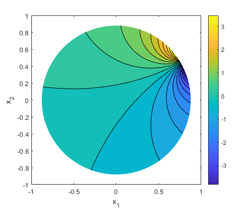
In this work, we assume that a dipole measurement can be made. By a dipole source, we mean the limiting boundary current of a source-sink pair when the distance between them goes to zero. For voltage measurement, we mean the limiting voltage between the same electrode. We provide a mathematical description of what we mean by measurement in Section 2. We assume that the anomaly in question is elliptical in shape. In the same section, the reader can find a description of the linearized forward map used in this work. In Section 3, we address the inverse problem of determining the anomaly location and size. We provide a direct method to solve the problem, and address uniqueness and stability. The question of what measurements to make, that is, optimal experiment design, is addressed in Section 4. We describe a Bayesian approach and a deterministic approach to find the optimal experiment design. We compare these two approaches in numerical simulations. Section 5 is devoted to the case where we attempt to fully characterize the elliptical anomaly. We find that the problem is unstable. Only the location and size of the anomaly can be robustly estimated. The paper concludes with a discussion section.
2 Linearized forward map
We begin by describing the model-to-data relationship in this inverse problem. We are interested in determining the geometric properties of a conductivity anomaly inside a domain which is a unit circle. We assume that the conductivity of the medium is given by
where is a small constant, and is a characteristic function supported on . We further assume that . The voltage potential caused by external sources is denoted by . Under linearization, , and the components satisfy
| (1) | |||||
| (2) |
The so-called background potential is caused by applied currents. The classical Calderon identity states that for a harmonic function , the following holds
| (3) |
We use polar coordinate ; our domain is the unit circle . We start by considering a current source-sink pair on the boundary as in Figure 1. A current source is located at and a current sink at . For measurement, the voltage difference between and is taken. In this case, the boundary condition for is
| (4) |
In this work, we will focus on dipole sources. This corresponds to the source-sink pair when we divide the right-hand side of (4) by and set it to zero. For a dipole source located at , the boundary condition for is
| (5) |
For measurement, the tangential derivative of the voltage is measured at . Thus, when the dipole is at angle , the measured data is . We set for uniqueness.
The background voltage potential satisfying (5) is given by [14]
| (6) |
In (3), we also choose so that the left-hand side is the tangential derivative of at the source location, namely,
where the tangential derivative is calculated using polar coordinates. Identifying the left-hand side as data, we identify the forward map, which depends on the measurement angle , as
| (7) |
The inverse problem is to find , properly parameterized, from measurement of the tangential derivative of at for several . To be more precise, we wish to find the parameters describing by solving the equation
| (8) |
Remark.
In practice, one could generate data with a source-sink pair very near each other; i.e., small in Figure 1. The measured voltage difference can be viewed as impedance between points and using Ohm’s law. Such resistance could be converted back into voltage difference since is known.
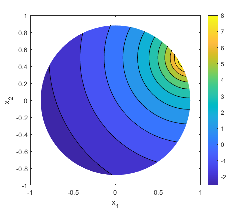
We next calculate the integrand in (7). By direct calculation, we can show that
| (9) |
The dipole potential field in (6) and its corresponding kernel in (9) are visualized in Figure 2.
For the remainder of this paper, we will assume that is a small elliptical domain. It is parameterized by the location of the center, , the semi-major and semi-minor axes, , and the orientation . The area of the ellipse is which is small by assumption. To obtain the forward map (7), we simply integrate for a given measurement angle over the ellipse.
We let . For a source located at , we have
| (10) |
From this, we can calculate
We can calculate second derivatives
In order to integrate over the ellipse, we use the quadratic approximation of at
| (11) | |||
Now, we set up the coordinates so that is aligned with the major axis of the ellipse, and the origin is at . Therefore
Let the orthogonal transformation be given by
Define
Then in (11) becomes
We find
Integrating over the ellipse, we get
| (13) |
One can check that in the case of a circle, i.e., , the last two terms become
and is independent of the orientation .
We can separate the terms that depend on the center and those that involve the ellipse and . We have
| (14) |
where
Having derived the forward map, we can now pose the inverse problem. We seek to find , , and , from the equations
| (15) |
where the forward map is given in (13) and are measurements. A simpler problem is one where the goal is to locate the center of the ellipse and its area . In this problem, the forward map is obtained after we drop the second order terms in the Taylor’s expansion of (11). Therefore, we have
| (16) |
where . We will consider both problems.
2.1 An alternate forward map using polarization tensors
A different approach to relating anomalies to boundary potential perturbations was first proposed in [4]. It is based on an asymptotic expansion that exploits smallness of the anomaly, rather than linearization around small conductivity contrast. For the problem at hand, we use the result in [2], Theorem 2.1. Writing the perturbed potential as and the background potential as , we have
| (17) |
where as in above, locates the center of the ellipse. In (17), is the Neumann function and is the background potential. Here is the size of the anomaly. For our purpose, we can set to 1 as long as the axes of the ellipse, are small. The geometric properties of the anomaly is encoded in the polarization tensor for an ellipse is given by
where
and is the orientation of the ellipse as before.
The gradient of the Neumann function in (17) the case of the unit circle is given by [2]
| (18) |
where . We wish to evaluate the tangential derivative of on the boundary. We write and directly calculate , which we will evaluate at . Noting that only depend on , we will work with (18). However, by direct calculation
which is the same as . Thus, we have
which agrees with (13).
3 Inversion for anomaly location and size
Suppose we put a dipole at angle and measure the corresponding tangential derivative of , namely . We do this for , with distinct. The inverse problem is to determine the location and the area of the anomaly from the measurements. We use the forward map in (16), so we have
| (19) |
3.1 Problem geometry
Define
| (20) |
The function is the squared distance from the anomaly center to the dipole located at . We see that
From the measurement, we can calculate
using the definition of . Expanding the above expression, we get
We can identify the center of the circle
It can be seen from the above formula that is on the line connecting and . Note that . For , is outside the unit circle and beyond , and for , it is beyond . Thus, the center cannot lie on the chord connecting the measurement points. The radius of the circle is
From the third measurement , we calculate
This too forms a circle with center at with
and radius . The center of the ellipse, is located at the intersection of the circle with center at with radius and the circle with center at with radius that lies inside the unit circle.
There are some interesting observations:
-
•
When , and , then and we get a straight line . Something similar occurs when , and . Then .
-
•
The circles get bigger if the center of the ellipse is away from a measurement point.
-
•
The radius grows linearly in the distance from the origin to the center of the ellipse.
Once the center of the ellipse is known, one can easily back out the area from the forward map.
Remark.
It would be desirable to have a way to characterize the range of the forward map. That is, given a data set, does there corresponds an ellipse whose location and size is consistent with the measured data? We were unable to find an easy characterization. However, it should be pointed that the constructive method described for calculating the center of the ellipse can be viewed as a way to characterize the range. If the data are out of range, the center of the ellipse would land outside the unit circle.
3.2 Unique determination of anomaly location and size
Theorem 1.
The anomaly location and size is uniquely determined by the data (16) if for and where is an integer.
Proof.
Let us assume that we have chosen for . The forward map takes the parameters to measurements according to the left-hand side of (19). That is
The Jacobian of the map can be shown to be
| (21) |
To prove uniqueness we will show that the determinant of the Jacobian is not zero. By direct calculation, we have
| (22) |
Expanding further, we get
after employing trigonometric identities. The numerator in the fraction is never zero, and . Thus, as long as the angles are distinct, the determinant never vanishes. ∎
Indeed, measurements from any three distinct are all that is needed to uniquely determine the location and size of the conductivity anomaly.
3.3 Stability
We investigate the stability of determining the center of the anomaly from measurements. For this purpose, we define the forward map based on the geometry of the problem
| (23) |
The Jacobian matrix is
| (24) |
where
The inverse of the Jacobian matrix is
| (25) |
Next, we examine the denominator in (25). To simplify matters, we set, without loss of generality, . Then we have
Further simplification shows that
From (25), we have
Recall from the definition of that
We can estimate the left-hand side with
By Cauchy-Schwarz inequality and the definition of
Similarly, . These lead to an estimate on the norm of the inverse of the Jacobian
Using the formula we obtained for the denominator, we arrive at
Theorem 2.
With the center of the ellipse at and dipole measurements taken at , , then the inverse of the Jacobian satisfies
| (26) |
Remark.
The estimate provides some insights into the stability. There are two terms in (2). We start with the second term. Since is the squared distance from dipole to the center of the anomaly, we can make this term small by placing the dipoles are close to the anomaly. However, to make the denominator in the first term large, we need to spread out the dipoles. Therefore, the two terms suggest that there is a tradeoff between closeness (measured by small ) and separateness (measured by the angular differences) of the measurement points. The factor implies that we must place one electrode close to the anomaly. We will revisit this issue when we examine optimal experiment design in the next section.
4 Optimal experiment design
4.1 Bayesian approach
In (19), we have discovered the expression of the data with respect to the measurement angle and the parameters, that is
| (27) | ||||
We now consider the problem in the Bayesian statistical framework. The measured data includes the normal noise ,
The prior distributions of the parameters are assumed to be normal
However, it should be noted that other prior distributions can be used. By taking measurements at , three realizations of are obtained, denoted as . Our task is to determine measurement locations whose associated posterior distributions of the parameters provide the most information. In other words, we want to choose that leads to the least amount of uncertainty in the parameters.
In [9], a utility function was introduced to quantify the information content about the parameters for a given a design. The utility function uses the Kullback-Leibler divergence, the discrepancy between the prior and the posterior given data to measure information gain
Denote as the utility of the design . Since the data can only be accessed after we have conducted the experiment, we take the expectation of the KL-divergence with respect to ’s distribution
The optimal design is found by maximizing the utility function over .
In computation, the expectation is approximated with Monte Carlo simulation
Here are sampled from and are sampled from . The denominator in the logarithm cannot be accessed directly, so an inner simulation is needed.
Similar as , are samples from . We write the inner and outer simulation together.
4.2 Numerical experiment with Bayesian approach.
Here we test the theory with simulations. We set the prior distributions of parameters as
The utility function is then maximized on the design space. For simplicity, we restrict our search to ‘symmetric designs’. That is, with the location as center, we constrain and by setting
This reduces the search space . We discretize the space and perform an exhaustive search in Figure 4. In practical settings, the optimization problem can be solved numerically using techniques like Bayesian Optimization. The means of the prior for , , and are , , and . The utility function has a maximum, and is periodic in .
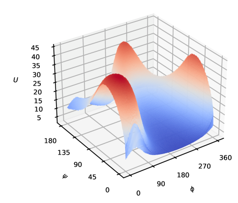
After finding the optimal and the worst experimental designs, we sample parameters from the prior distributions to obtain ‘ground-truth’ parameters: , , . We simulate the measurement process and produce data from the two designs. We compute the posterior distributions for them. Figures 5 display the posterior distribution for the three parameters. It is clear that the best design produces tighter distributions.
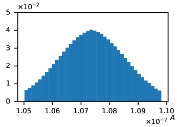
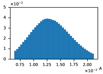
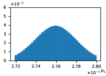
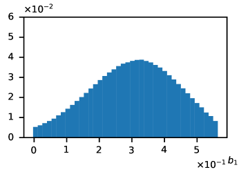

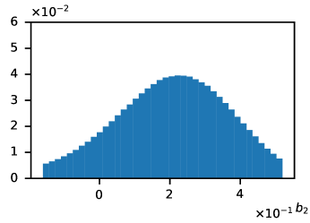
For both experiments, we compute the sample mean and 95% confidence bounds for the parameters, which we summarize below in Table 1.
| Experiment | parameters | mean | l.b. | u.b |
|---|---|---|---|---|
| Optimal | ||||
| Worst | ||||
4.3 Deterministic approach
In the deterministic approach for optimal experiment design, we consider the Jacobian in (21). Optimality is measured by how well-conditioned is for an a priori location , and area . To keep the numerical calculation consistent with the above example with the Bayesian approach, we set , , and . We again consider a symmetric design, so the design space is , and (). A proxy for optimality is the reciprocal of the condition number. The larger this number, the more stable the reconstruction around the a prior values.
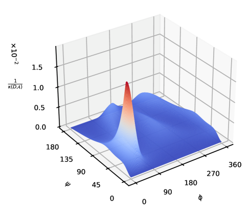
Figure 4 and Figure 6 shows some similarity. It should be pointed out that the assumptions in these two approaches are different. In the former, we assume we have priors, and the resulting utility are based on all possible priors. In the latter, the proxy for utility depends on the parameters themselves, which is counter to the nature of inverse problems. However, one can exploit the easy computation of the utility. One can start with an experiment design, estimate the parameters and the utility, based on these, update the experiment, i.e., move the electrode locations, until the maximum utility is as large as possible. This idea was explored in [13] in the context of imaging cracks using electrical impedance tomography.
5 Determination of an elliptical anomaly
We turn our attention to the problem of finding parameters of a small elliptical anomaly from measured dipole data. The forward map is given in (13) and the inverse problem is to find the ellipse center , its semi-major and semi-minor axes , and its orientation given data in
5.1 Jacobian
We will start by examining the structure of the Jacobian of the forward map. The following calculations will reveal that the problem is highly ill-posed. The findings of this section informs the computational method which we present in the following subsection.
Recall the takes the form
| (28) |
We will write and , where
and
Then the partial derivatives of (28):
We use as our order parameter. Then and are . We see that to leading order
The Jacobian matrix of the forward map will have columns whose magnitudes are
Since is small, the Jacobian, while it may be invertible, is very ill-conditioned. Therefore, we expect the stability of the inverse problem for the five parameters of the elliptical anomaly to be poor.
5.2 A Newton’s method for anomaly determination
From Section 3.4, we expect that the problem of determining the location and the size of the ellipse to be relatively well-posed, provided that the experiments are well designed. Therefore, we propose the following algorithm.
In the algorithm, since the Jacobian is ill-conditioned, we propose using the pseudo-inverse with a cut-off for the smallest singular value. The parameter is the step size. The vectors and are column vectors made up of the measurements at the five dipole locations.
5.3 Numerical experiments
For the purpose of understanding the behavior of the proposed Newton’s method for the recovery of the parameters of the elliptical anomaly, we perform some tests with simulated data. Noise is added to the data to assess the sensitivity of the reconstruction to data errors.
In all the experiments, the dipoles are located at angles . The ground truth values are , , , , and . The forward map is computed using (28). For noise, we add a mean-zero normally distributed random number with standard deviation that is a small multiple of . Thus, we are assuming that the perturbation from noise is proportional to the signal size. We will report the relative -norm of the noise.
| Step 1 | Step 2 | |||||||
|---|---|---|---|---|---|---|---|---|
| noise | ||||||||
| 0.40 | 0.50 | 0.01 | 0.40 | 0.50 | 0.08 | 0.04 | ||
| 0.40 | 0.50 | 0.01 | 0.40 | 0.50 | 0.09 | 0.04 | ||
| 0.39 | 0.49 | 0.01 | 0.40 | 0.49 | 0.11 | 0.03 | ||
| 0.40 | 0.50 | 0.01 | 0.40 | 0.50 | 0.12 | 0.03 | ||
| 0.40 | 0.49 | 0.01 | 0.40 | 0.50 | 0.10 | 0.03 | ||
The results of the numerical experiments are presented in Table 2. It is clear that the location and the area of the elliptical anomaly are well determined. Sensitivity in the determination of the parameters of the ellipse is higher, as predicted from the nature of the Jacobian matrix. In the experiments, we put a cutoff in the pseudo-inverse of – we drop singular vectors corresponding singular values below . With this cutoff, the algorithm may diverge depending on noise level. Higher cutoff will stabilize the algorithm at the cost of increased loss of accuracy. We did not fully explore the interplay between noise level and the cutoff value.
6 Discussion
In this work, we examined electrical impedance tomography with minimal measurements. Of interest is the recovery of a small, elliptical conductivity anomaly with small conductivity contrast against a constant background. We show that while finding the location and size of the anomaly is quite stable, the determination of the axes of the ellipse and its orientation is numerically challenging.
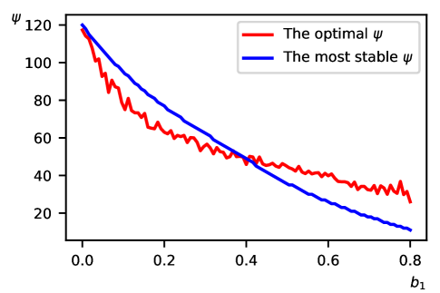
We also investigated the question of optimal experiment design in the context of Bayesian statistics. We find that if we have a prior on the location and size of the ellipse, we can find the optimal places on the boundary at which measurements should be made. A deterministic approach to optimal experiment design is explored. Here, the outcome depends on the location and size of the ellipse. If we have a prior, then we can use the means as input to find the optimal measurement locations. That the two approaches to optimal experiment design are roughly equivalent can be seen in Figure 7. We set and choose . The only design parameter remaining is . Shown in the figure are the angle from the Bayesian approach as a function of the mean in the prior and from the deterministic approach. While the difference is small, what is clear is that optimal experiment design has an important role to play in this problem.
Acknowledgements
Gaoming Chen’s participation in this work was made possible by the Visiting Student Program at Johns Hopkins University. He thanks the many professors and graduate students who made his visit during the Fall of 2023 most enjoyable.
References
References
- [1] L. Borcea, Electrical impedance tomography, Inverse Problems 18 (2002), R99-R136.
- [2] M. Bruhl, M. Hanke, and M. Vogelius, A direct impedance tomography algorithm for locating small inhomogeneities, Numerische Mathematik, 93 (2003), 635-654.
- [3] A. Calderon, On an inverse boundary value problem, Seminar on Numerical Analysis and its Applications to Continuum Physics (Rıo de Janeiro, 1980), pp. 65–73, Soc. Brazil. Mat., Rio de Janeiro, 1980.
- [4] D. Cedio-Fengya, D. Moskow, and M. Vogelius, Identification of conductivity imperfections of small diameter by boundary measurements. Continuous dependence and computational reconstruction, Inverse Problems, 14 (1998), 553-595.
- [5] A. Friedman and V. Isakov, On the uniqueness in the inverse conductivity problem with one measurement, Indiana Univ. Math. J. 38 (1989), 563-579.
- [6] A. Friedman and M. Vogelius, Determining cracks by boundary measurements, Indiana Mathematics Journal 38 (1989), 497-525.
- [7] V. Isakov and A. Titi, Stability and the inverse gravimetry problem with minimal data, J. Inverse and Ill-posed Problems, 30 (2022), 147-162.
- [8] V. Isakov and A. Titi, On the inverse gravimetry problem with minimal data, J. Inverse and Ill-posed Problems, 32 (2022), 807-822.
- [9] X. Huan and Y. Marzouk, Simulation-based optimal Bayesian experimental design for nonlinear systems, Journal of Computational Physics, 232 (2013), 288-317.
- [10] J. Kaipio and E. Somersalo, Statistical and Computational Inverse Problems, Springer, 2010.
- [11] A. Karageorghis and D. Lesnic, Reconstruction of an elliptical inclusion in the inverse conductivity problem, Int. J. Mechanical Sciences 142-143 (2018), 603-609.
- [12] O. Kwon, J. Yoon, J. Seo, E. Woo, Estimation of anomaly location and size using electrical impedance tomography, IEEE Trans. Biomed. Eng., 50 (2003), 89-96.
- [13] F. Santosa and M. Vogelius, A computational algorithm to determine cracks from electrostatic boundary measurements, Int. J Engng. Sci, 29 (1991), 917-937.
- [14] F. Santosa and M. Vogelius, A backprojection algorithm for electrical impedance tomography, SIAM J. Appl. Math., 50 (1990), 216-243.