Hybrid Feedback for Three-dimensional Convex Obstacle Avoidance

Abstract

We propose a hybrid feedback control scheme for the autonomous robot navigation problem in three-dimensional environments with arbitrarily-shaped convex obstacles. The proposed hybrid control strategy, which consists in switching between the move-to-target mode and the obstacle-avoidance mode, guarantees global asymptotic stability of the target location in the obstacle-free workspace. We also provide a procedure for the implementation of the proposed hybrid controller in a priori unknown environments and validate its effectiveness through simulation results.

I Introduction

Safe autonomous robot navigation consists in steering a robot to a target location while avoiding obstacles. One commonly used navigation technique is the Artificial Potential Field (APF) approach [1], where a combination of attractive and repulsive vector fields guides the robot safely to the target location. However, this approach faces challenges with certain obstacle arrangements, leading to undesired local minima. The Navigation Function (NF) approach [2] is effective in sphere world environments [3, 4], addressing the local minima issue by limiting the repulsive field’s influence around the obstacles by means of a properly tuned parameter. This method ensures almost global convergence of the robot to the target location. To apply the NF approach to environments with general convex and star-shaped obstacles, diffeomorphic mappings from [3] and [5] can be used. However, these mappings require global knowledge of the environment for implementation. The NF-based approach has been extended in [6] to environments containing convex obstacles with smooth boundaries. The authors established sufficient conditions on the curvature of the obstacles’ boundaries to guarantee almost global convergence to a neighborhood surrounding the a priori unknown target location. However, it is assumed that the shapes of the obstacles avoided by the robot are known.

In [7], the authors proposed a feedback controller based on Nagumo’s theorem [8, Theorem 4.7], for autonomous navigation in environments with general convex obstacles. The forward invariance of the obstacle-free space is ensured by projecting the ideal velocity control vector (pointing to the target) onto the tangent cone at the boundary of the obstacle whenever it points to the obstacle. In [9], a control barrier function-based approach was used for robot navigation in an environment with a single spherical obstacle. In [10], the authors proposed a separating hyperplane-based autonomous navigation algorithm for the robot navigating in environments with convex obstacles with smooth boundaries. This approach was extended in [11] to handle partially known environments with non-convex obstacles, where it is assumed that the robot possesses geometrical information about the non-convex obstacles but lacks knowledge of their precise locations in the workspace. However, due to the topological obstruction to global asymptotic stability, with continuous time-invariant vector fields, in sphere words [2], the above-mentioned approaches provide at best almost global asymptotic stability guarantees.
In [12], hybrid control techniques were employed to achieve global stabilization of the target location in environments with sufficiently separated ellipsoidal obstacles. In [13], the authors utilized the hybrid control techniques to propose an autonomous navigation technique for a nonholonomic robot operating in environments with non-convex obstacles under some restrictions on the inter-obstacle arrangements. In [14], the authors proposed a discontinuous feedback control law for autonomous robot navigation in partially known two-dimensional environments. When a known obstacle is encountered, the control vector aligns with the negative gradient of the navigation function. However, when close to an unknown obstacle, the robot moves along its boundary, relying on the local curvature information of the obstacle. Similar to [13], this approach is applicable to two-dimensional environments and assumes smooth obstacle boundaries without sharp edges. In our earlier work [15], we proposed a hybrid feedback control strategy to address the problem of autonomous robot navigation in two-dimensional environments with arbitrarily-shaped convex obstacles.
In this paper, we propose a hybrid control strategy, endowed with global asymptotic stability guarantees, for autonomous robot navigation in three-dimensional environments with arbitrarily-shaped convex obstacles that can have non-smooth boundaries. We also propose a sensor based version of our approach for autonomous navigation in a priori unknown three-dimensional environments with arbitrarily-shaped convex obstacles.

II Notations and Preliminaries

II-A Notations

The sets of real and natural numbers are denoted by $\mathbb{R}$ and $\mathbb{N}$, respectively. We identify vectors using bold lowercase letters. The Euclidean norm of a vector $\mathbf{p}\in\mathbb{R}^{n}$ is denoted by $\lVert\mathbf{p}\rVert$, and an Euclidean ball of radius $r\geq 0$ centered at $\mathbf{p}$ is represented by $\mathcal{B}_{r}(\mathbf{p})=\{\mathbf{q}\in\mathbb{R}^{n}|\lVert\mathbf{q}-\mathbf{p}\rVert\leq r\}.$ The set of $n-$dimensional unit vectors is given by $\mathbb{S}^{n-1}=\{\mathbf{p}\in\mathbb{R}^{n}|\lVert\mathbf{p}\rVert=1\}.$ The three-dimensional Special Orthogonal group is defined by $SO(3):=\{\mathbf{R}\in\mathbb{R}^{3\times 3}:\mathbf{R}^{\top}\mathbf{R}=\mathbf{R}\mathbf{R}^{\top},\det(\mathbf{R})=1\}.$ For a given vector $\mathbf{x}:=[x_{1},x_{2},x_{3}]^{\top}\in\mathbb{R}^{3}$, we define $\mathbf{x}^{\times}$ as the skew-symmetric matrix, which is given by

$$\mathbf{x}^{\times}=\begin{bmatrix}0&-x_{3}&x_{2}\\ x_{3}&0&-x_{1}\\ -x_{2}&x_{1}&0\end{bmatrix}.$$ (1)

For two sets $\mathcal{A},\mathcal{B}\subset\mathbb{R}^{n}$, the relative complement of $\mathcal{B}$ with respect to $\mathcal{A}$ is denoted by $\mathcal{A}\setminus\mathcal{B}=\{\mathbf{a}\in\mathcal{A}|\mathbf{a}\notin\mathcal{B}\}$. The symbols $\partial\mathcal{A},\mathcal{A}^{\circ}$, $\mathcal{A}^{c}$ and $\bar{\mathcal{A}}$ represent the boundary, interior, complement and the closure of the set $\mathcal{A}$, respectively, where $\partial\mathcal{A}=\bar{\mathcal{A}}\backslash\mathcal{A}^{\circ}$. The cardinality of a set $\mathcal{A}$ is denoted by $\mathbf{card}(\mathcal{A})$. The Minkowski sum of the sets $\mathcal{A}$ and $\mathcal{B}$ is denoted by, $\mathcal{A}\oplus\mathcal{B}=\{\mathbf{a}+\mathbf{b}|\mathbf{a}\in\mathcal{A},\mathbf{b}\in\mathcal{B}\}$. The dilated version of a set $\mathcal{A}\subset\mathbb{R}^{n}$ with $r\geq 0$ is represented by $\mathcal{D}_{r}(\mathcal{A})=\mathcal{A}\oplus\mathcal{B}_{r}(\mathbf{0})$. The $r-$neighbourhood of a set $\mathcal{A}$ is denoted by $\mathcal{N}_{r}(\mathcal{A})=\mathcal{D}_{r}(\mathcal{A})\setminus\mathcal{A}^{\circ}$ where $r$ is a strictly positive scalar.

II-B Projection on a set

Given a closed set $\mathcal{A}\subset\mathbb{R}^{n}$ and a point $\mathbf{x}\in\mathbb{R}^{n}$, the Euclidean distance of $\mathbf{x}$ from the set $\mathcal{A}$ is evaluated as

$$d(\mathbf{x},\mathcal{A})=\underset{\mathbf{q}\in\mathcal{A}}{\min}\lVert\mathbf{x}-\mathbf{q}\rVert.$$ (2)

The set $\mathcal{PJ}(\mathbf{x},\mathcal{A})\subset\mathcal{A}$, which is defined as

$$\mathcal{PJ}(\mathbf{x},\mathcal{A})=\{\mathbf{q}\in\mathcal{A}|\lVert\mathbf{x}-\mathbf{q}\rVert=d(\mathbf{x},\mathcal{A})\},$$ (3)

is the set of points in $\mathcal{A}$ that are at the distance of $d(\mathbf{x},\mathcal{A})$ from $\mathbf{x}$. If $\mathbf{card}(\mathcal{PJ}(\mathbf{x},\mathcal{A}))$ is one, then the element of the set $\mathcal{PJ}(\mathbf{x},\mathcal{A})$ is denoted by $\Pi(\mathbf{x},\mathcal{A})$.

II-C Geometric subsets of $\mathbb{R}^{n}$

II-C1 Line segment

The line segment joining two points $\mathbf{p}\in\mathbb{R}^{n}$ and $\mathbf{q}\in\mathbb{R}^{n}$ is given by

$$\mathcal{L}_{s}(\mathbf{p},\mathbf{q}):=\{\mathbf{x}\in\mathbb{R}^{n}|\mathbf{x}=\lambda\mathbf{p}+(1-\lambda)\mathbf{q},\lambda\in[0,1]\}.$$ (4)

II-C2 Hyperplane

The hyperplane passing through $\mathbf{p}\in\mathbb{R}^{n}$ and orthogonal to $\mathbf{q}\in\mathbb{R}^{n}\backslash\{\mathbf{0}\}$ is given by

$$\mathcal{P}(\mathbf{p},\mathbf{q}):=\{\mathbf{x}\in\mathbb{R}^{n}|\mathbf{q}^{\intercal}(\mathbf{x}-\mathbf{p})=0\}.$$ (5)

The hyperplane divides the Euclidean space $\mathbb{R}^{n}$ into two half-spaces i.e., a closed positive half-space $\mathcal{P}_{\geq}(\mathbf{p},\mathbf{q})$ and a closed negative half-space $\mathcal{P}_{\leq}(\mathbf{p},\mathbf{q})$ which are obtained by substituting ‘$=$’ with ‘$\geq$’ and ‘$\leq$’ respectively, in the right-hand side of (5). We also use the notations $\mathcal{P}_{>}(\mathbf{p},\mathbf{q})$ and $\mathcal{P}_{<}(\mathbf{p},\mathbf{q})$ to denote the open positive and the open negative half-spaces such that $\mathcal{P}_{>}(\mathbf{p},\mathbf{q})=\mathcal{P}_{\geq}(\mathbf{p},\mathbf{q})\backslash\mathcal{P}(\mathbf{p},\mathbf{q})$ and $\mathcal{P}_{<}(\mathbf{p},\mathbf{q})=\mathcal{P}_{\leq}(\mathbf{p},\mathbf{q})\backslash\mathcal{P}(\mathbf{p},\mathbf{q})$.

II-D Hybrid system framework

A hybrid dynamical system [16] is represented using differential and difference inclusions for the state $\mathbf{\xi}\in\mathbb{R}^{n}$ as follows:

$$\begin{cases}\begin{matrix}\mathbf{\dot{\xi}}\in\mathbf{F}(\mathbf{\xi}),&\mathbf{\xi}\in\mathcal{F},\\ \mathbf{\xi}^{+}\in\mathbf{J}(\mathbf{\xi}),&\mathbf{\xi}\in\mathcal{J},\end{matrix}\end{cases}$$ (6)

where the flow map $\mathbf{F}:\mathbb{R}^{n}\rightrightarrows\mathbb{R}^{n}$ is the differential inclusion which governs the continuous evolution when $\mathbf{\xi}$ belongs to the flow set $\mathcal{F}\subseteq\mathbb{R}^{n}$, where the symbol ‘$\rightrightarrows$’ represents set-valued mapping. The jump map $\mathbf{J}:\mathbb{R}^{n}\rightrightarrows\mathbb{R}^{n}$ is the difference inclusion that governs the discrete evolution when $\mathbf{\xi}$ belongs to the jump set $\mathcal{J}\subseteq\mathbb{R}^{n}$. The hybrid system (6) is defined by its data and denoted as $\mathcal{H}=(\mathcal{F},\mathbf{F},\mathcal{J},\mathbf{J}).$

A subset $\mathbb{T}\subset\mathbb{R}_{\geq}\times\mathbb{N}$ is a hybrid time domain if it is a union of a finite or infinite sequence of intervals $[t_{j},t_{j+1}]\times\{j\},$ where the last interval (if existent) is possibly of the form $[t_{j},T)$ with $T$ finite or $T=+\infty$. The ordering of points on each hybrid time domain is such that $(t,j)\preceq(t^{\prime},j^{\prime})$ if $t\leq t^{\prime}$ and $j\leq j^{\prime}$. A hybrid solution $\phi$ is maximal if it cannot be extended, and complete if its domain dom $\phi$ (which is a hybrid time domain) is unbounded.

III Problem Formulation

We consider a spherical robot with radius $r\geq 0$ operating in a convex, three-dimensional Euclidean space $\mathcal{W}\subseteq\mathbb{R}^{3}.$ The workspace $\mathcal{W}$ is cluttered with finite number of compact, convex obstacles $\mathcal{O}_{i}\subset\mathcal{W},i\in\{1,\ldots,b\},b\in\mathbb{N}.$ We define obstacle $\mathcal{O}_{0}:=(\mathcal{W}^{\circ})^{c}$ as the complement of the interior of the workspace. Collectively, the obstacle-occupied workspace is denoted by $\mathcal{O}_{\mathcal{W}}=\bigcup_{i\in\mathbb{I}}\mathcal{O}_{i}$, where $\mathbb{I}=\{0,\ldots,b\}.$ We make the following workspace feasibility assumption:

Assumption 1.

The minimum separation between any pair of obstacles should be greater than $2r$ i.e., for all $i,j\in\mathbb{I},i\neq j,$ one has

$$d(\mathcal{O}_{i},\mathcal{O}_{j}):=\underset{\mathbf{p}\in\mathcal{O}_{i},\mathbf{q}\in\mathcal{O}_{j}}{\text{min}}\|{\mathbf{p}-\mathbf{q}}\|>2r.$$ (7)

According to Assumption 7 and the compactness of the obstacles, there exists a minimum separating distance between any pair of obstacles $\bar{r}=\underset{i,j\in\mathbb{I},i\neq j}{\min}d(\mathcal{O}_{i},\mathcal{O}_{j})>2r$. Moreover, for collision-free navigation we require $d(\mathbf{0},\mathcal{O}_{\mathcal{W}})-r>0$. We define a positive real $\bar{r}_{s}$ as

$$\bar{r}_{s}=\underset{}{\min}\left\{\frac{\bar{r}}{2}-r,d(\mathbf{0},\mathcal{O}_{\mathcal{W}})-r\right\}.$$ (8)

We then pick an arbitrarily small value $r_{s}\in(0,\bar{r}_{s})$ as the minimum distance that the robot should maintain with respect to any obstacle.

The obstacle-free workspace is then defined as $\mathcal{W}_{0}:=\mathcal{W}\setminus\mathcal{O}_{\mathcal{W}}.$ Given $y\geq 0$, a $y-$eroded obstacle-free workspace, $\mathcal{W}_{y}$ is defined as

$$\mathcal{W}_{y}:=\mathcal{W}\setminus\bigcup_{i\in\mathbb{I}}\mathcal{D}_{y}^{\circ}(\mathcal{O}_{i})\subseteq\mathcal{W}_{0}.$$ (9)

Hence, $\mathcal{W}_{r_{a}}$ with $r_{a}=r+r_{s}$ is the obstacle-free workspace with respect to the center of the robot i.e., $\mathbf{x}\in\mathcal{W}_{r_{a}}\iff\mathcal{B}_{r_{a}}(\mathbf{x})\subset\mathcal{W}_{0}.$

The robot is governed by a single integrator dynamics

$$\dot{\mathbf{x}}=\mathbf{u},$$ (10)

where $\mathbf{u}\in\mathbb{R}^{3}$ is the control input. The task is to design a feedback control law $\mathbf{u}$ such that:

1. Safety: the robot-centered obstacle-free workspace $\mathcal{W}_{r_{a}}$ is forward invariant,

2. Global Asymptotic Stability: Any given target location $\mathbf{x}=\mathbf{0}\in\mathcal{W}_{r_{a}}^{\circ}$ is a globally asymptotically stable equilibrium for the closed-loop system.

IV Hybrid Control For Obstacle Avoidance

In the proposed scheme, the robot operates in two modes based on the value of a mode indicator variable $m\in\mathbb{M}:=\{0,1\}$. The move-to-target mode $(m=0)$ is adopted when the robot is away from the obstacles and the the obstacle-avoidance mode $(m=1)$ is adopted when the robot is close to an obstacle obstructing its motion towards the target location. In the move-to-target mode, the robot moves straight towards the target location. In the obstacle-avoidance mode, the robot navigates around the obstacle while staying withing its $\gamma-$neighborhood, where $\gamma\in(0,\bar{r}_{s}-r_{s})$. When the robot operates in the obstacle-avoidance mode, the robot’s center has a unique closest point on the nearest obstacle. Furthermore, to prevent the robot from getting trapped in a loop around an obstacle, the proposed obstacle-avoidance strategy confines the robot’s center to a hyperplane that passes through the target location. This ensures that the robot will eventually reach a position where the nearest obstacle does not intersect with the line segment joining the center of the robot and the target location.

IV-A Hybrid control design

The proposed hybrid control $\mathbf{u}(\mathbf{x},\mathbf{h},\mathbf{a},m,s)$ is given as

$$\mathbf{u}(\xi)=-\kappa_{s}(1-m)\mathbf{x}+\kappa_{r}m\mathbf{v}(\mathbf{x},\mathbf{a}),$$ (11a)

$$\underbrace{\begin{matrix}\mathbf{\dot{h}}\\ \mathbf{\dot{a}}\\ \dot{m}\\ \dot{s}\end{matrix}\begin{matrix}\;=\mathbf{0},\\ \;=0,\\ \;=0\\ \;=1,\end{matrix}}_{(\mathbf{x},\mathbf{h},\mathbf{a},m,s)\in\mathcal{F}}\quad\quad\underbrace{\begin{bmatrix}\mathbf{h^{+}}\\ \mathbf{a^{+}}\\ m^{+}\\ {s^{+}}\end{bmatrix}\begin{matrix}\;\in\mathbf{L}(\mathbf{x},\mathbf{h},\mathbf{a},m,s),\end{matrix}}_{(\mathbf{x},\mathbf{h},\mathbf{a},m,s)\in\mathcal{J}}$$ (11b)

where $\kappa_{s}>0$, $\kappa_{r}>0$, and $\xi=(\mathbf{x},\mathbf{h},\mathbf{a},m,s)\in\mathcal{K}:=\mathcal{W}_{r_{a}}\times\mathcal{W}_{r_{a}}\times\mathbb{S}^{2}\times\mathbb{M}\times\mathbb{R}_{\geq 0}$. The variable $\mathbf{h}$ denotes the hit point, which is the location where the robot switches from the move-to-target mode to the obstacle-avoidance mode. The vector $\mathbf{a}\in\mathbb{S}^{2}$ is instrumental for the construction of the avoidance control vector $\mathbf{v}(\mathbf{x},\mathbf{a})$, used in (11a). The scalar variable $s\in\mathbb{R}_{\geq 0}$ allows the robot to switch from the obstacle-avoidance mode to the move-to-target mode when initially in the obstacle-avoidance mode. Details of this switching process are provided later in Section IV-B. The sets $\mathcal{F}$ and $\mathcal{J}$ are the flow and jump sets related to different modes of operation, respectively, whose constructions are provided in Section IV-B. The update law $\mathbf{L}$, which allows the robot to update the values of the variables $\mathbf{h}$, $\mathbf{a}$, and $m$ based on the current location of the robot with respect to the nearest obstacle and the target location, will be designed later in Section IV-C. Next, we provide the design of the vector $\mathbf{v}(\mathbf{x},\mathbf{a})\in\mathbb{R}^{3}$.

The vector $\mathbf{v}(\mathbf{x},\mathbf{a}),$ used in (11a), is defined as

$$\mathbf{v}(\mathbf{x},\mathbf{a})=\big{[}\eta(\mathbf{x})\mathbf{I}+(1-|\eta(\mathbf{x})|)\mathbf{R}(\mathbf{a})\big{]}{{\mathbf{P}(\mathbf{a})\mathbf{x}_{\pi}}}$$ (12)

where $\mathbf{I}\in\mathbb{R}^{3\times 3}$ is the identity matrix and $\mathbf{x}_{\pi}:=\mathbf{x}-\Pi(\mathbf{x},\mathcal{O}_{\mathcal{W}}).$ The operator $\Pi(\mathbf{x},\mathcal{O}_{\mathcal{W}})$ provides the closest point on the obstacle-occupied workspace from the location of the center of the robot $\mathbf{x}$, as defined in Section II-B. Notice that, since the obstacles $\mathcal{O}_{i},i\in\mathbb{I}\setminus\{0\}$ are convex and the parameter $\gamma\in(0,\bar{r}_{s}-r_{s})$, according to (8), the robot will have a unique closest point to the obstacles whenever its center is in the $(r_{a}+\gamma)-$neighborhood of these obstacles. On the other hand, there may be some locations in the $(r_{a}+\gamma)-$neighborhood of the obstacle $\mathcal{O}_{0}=(\mathcal{W}^{\circ})^{c}$ for which the uniqueness of the closest point from robot’s center to the obstacle $\mathcal{O}_{0}$ cannot be guaranteed. However, as discussed later in Remark 1, the design of the flow sets and jump sets guarantees that the obstacle-avoidance control vector $\mathbf{v}(\mathbf{x},\mathbf{a})$ is never activated in the region $\mathcal{N}_{r_{a}+\gamma}(\mathcal{O}_{0}).$

The rotation matrix $\mathbf{R}(\mathbf{a}):=\mathcal{R}(\frac{\pi}{2},\mathbf{a})\in SO(3)$, with $\mathcal{R}(\theta,\mathbf{a})$ being the rotation by an angle $\theta$ about the unit vector $\mathbf{a}$, defined as follows:

$$\mathcal{R}(\theta,\mathbf{a}):=\mathbf{I}_{3}+\sin(\theta)\mathbf{a}^{\times}+(1-\cos(\theta))(\mathbf{a}^{\times})^{2},$$

which, for $\theta=\frac{\pi}{2}$, leads to

$$\mathbf{R}(\mathbf{a})=\mathbf{a}\mathbf{a}^{\top}+\mathbf{a}^{\times},$$

where we used the fact that $(\mathbf{a}^{\times})^{2}=\mathbf{a}\mathbf{a}^{\top}-I$, with $\mathbf{a}^{\times}$ being the skew-symmetric matrix associated to the unit vector $\mathbf{a}=[a_{1}~{}a_{2}~{}a_{3}]^{\top}$, defined according to (1).

The matrix $\mathbf{P}(\mathbf{a})\in\mathbb{R}^{3\times 3}$, which is used in (12), is given by

$$\mathbf{P}(\mathbf{a}):=\mathbf{I}_{3}-\frac{\mathbf{a}\mathbf{a}^{\intercal}}{\lVert\mathbf{a}\rVert^{2}}.$$ (13)

For any vector $\mathbf{x}\in\mathbb{R}^{3},$ the vector $\mathbf{P}(\mathbf{a})\mathbf{x}$ corresponds to the projection of $\mathbf{x}$ onto the hyperplane orthogonal to $\mathbf{a}$. As discussed later in Section IV-C, the coordinates of the unit vector $\mathbf{a}$ are updated when the robot switches from the move-to-target mode to the obstacle-avoidance mode according to the update law $\mathbf{L}(\xi)$, whose design is provided later in Section IV-C.

Finally, the scalar function $\eta(\mathbf{x})\in[0,1]$ is given by

$$\eta(\mathbf{x})=\begin{cases}-1,&d(\mathbf{x},\mathcal{O}_{\mathcal{W}})-r_{a}\geq\gamma_{s},\\ 1-\frac{d(\mathbf{x},\mathcal{O}_{\mathcal{W}})-r_{a}-\gamma_{a}}{0.5(\gamma_{s}-\gamma_{a})},&\gamma_{a}\leq d(\mathbf{x},\mathcal{O}_{\mathcal{W}})-r_{a}\leq\gamma_{s},\\ 1,&d(\mathbf{x},\mathcal{O}_{\mathcal{W}})-r_{a}\leq\gamma_{a},\end{cases}$$ (14)

where $0<\gamma_{a}<\gamma_{s}<\gamma.$ The scalar function $\eta$ is designed to ensure that the center of the robot remains inside the $\gamma-$neighborhood of the $r_{a}-$dilated obstacle-occupied workspace $\mathcal{N}_{\gamma}(\mathcal{D}_{r_{a}}(\mathcal{O}_{\mathcal{W}}))$ when it operates in the obstacle-avoidance mode in the set $\mathcal{N}_{\gamma}(\mathcal{D}_{r_{a}}(\mathcal{O}_{\mathcal{W}}))$. This feature allows for the design of the jump set of the obstacle-avoidance mode, as discussed later in Section IV-B2, and ensures convergence to the target location, as stated later in Theorem 1. Next, we provide the construction of the flow set $\mathcal{F}$ and the jump set $\mathcal{J}$ used in (11).

IV-B Geometric construction of the flow and jump sets

When the robot operates in the move-to-target mode, its velocity is directed towards the target location. Hence, if the path joining the robot’s location and the target is obstructed by an obstacle, let’s say $\mathcal{O}_{i}$ for some $i\in\mathbb{I}$ i.e., $\mathcal{L}_{s}(\mathbf{x},\mathbf{0})\cap\mathcal{D}_{r_{a}}^{\circ}(\mathcal{O}_{i})\neq\emptyset$, then the center of the robot enters the $(r_{a}+\gamma)-$neighbourhood of the obstacle $\mathcal{O}_{i}$ through the landing region $\mathcal{R}_{l}^{i},$ which is defined as

$$\mathcal{R}_{l}^{i}:=\left\{\mathbf{x}\in\mathcal{N}_{\gamma}(\mathcal{D}_{r_{a}}(\mathcal{O}_{i}))|{\mathcal{L}_{s}(\mathbf{x},\mathbf{0})}\cap\mathcal{D}_{r_{a}}^{\circ}(\mathcal{O}_{i})\neq\emptyset\right\}.$$ (15)

The union of the landing regions over all obstacles is defined as

$$\mathcal{R}_{l}:=\bigcup_{i\in\mathbb{I}}\mathcal{R}_{l}^{i}.$$ (16)

Next, we define an exit region $\mathcal{R}_{e}$ as the part of the $\gamma-$neighborhood of the $r_{a}-$dilated obstacles that do not belong the landing region. The exit region $\mathcal{R}_{e}$ is defined as

$$\mathcal{R}_{e}=\mathcal{N}_{\gamma}(\mathcal{D}_{r_{a}}(\mathcal{O}_{\mathcal{W}}))\setminus\mathcal{R}_{l}.$$ (17)

Note that when the robot’s center at $\mathbf{x}$ belongs to the exit region, the line segment connecting its location to the target location $\mathcal{L}_{s}(\mathbf{x},\mathbf{0})$ does not intersect with the interior of the nearest $r_{a}-$dilated obstacle. Hence, the robot should move straight towards the target location only if it is in the exit region. Next, we provide the geometric construction of the flow set $\mathcal{F}$ and the jump set $\mathcal{J}$, used in (11).

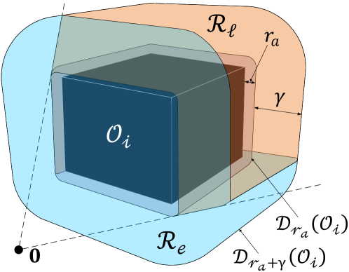
Figure 1: The geometrical representation of the landing region and the exit region.

IV-B1 Flow and jump sets (move-to-target mode)

When the robot operating in the move-to-target mode, enters in the landing region $\mathcal{R}_{l}$ (16), it should switch to the obstacle-avoidance mode to avoid collision. Hence, the jump set of the move-to-target mode for the state $\mathbf{x}$ is defined as

$$\mathcal{J}_{0}^{\mathcal{W}}:=\overline{\mathcal{N}_{\gamma_{s}}(\mathcal{D}_{r_{a}}(\mathcal{O}_{\mathcal{W}}))\cap\mathcal{R}_{l}},$$ (18)

where $\gamma_{s}\in(0,\gamma).$ For robustness purposes (with respect to noise), we introduce a hysteresis region by allowing the robot, operating in the move-to-target mode inside the $(r_{a}+\gamma)-$neighbourhood of the set $\mathcal{O}_{\mathcal{W}}$, to move closer to the set $\mathcal{O}_{\mathcal{W}}$ before switching to the obstacle-avoidance mode.

The flow set of the move-to-target mode for the state $\mathbf{x}$ is then defined as

$$\mathcal{F}_{0}^{\mathcal{W}}:=\left(\mathcal{W}\setminus(\mathcal{D}_{r_{a}+\gamma_{s}}^{\circ}(\mathcal{O}_{\mathcal{W}}))\right)\cup\mathcal{R}_{e}.$$ (19)

Notice that the union of the jump set $\mathcal{J}_{0}^{\mathcal{W}}$ and the flow set $\mathcal{F}_{0}^{\mathcal{W}}$ covers the robot-centered obstacle-free workspace $\mathcal{W}_{r_{a}}$.

The flow set $\mathcal{F}_{0}$ and the jump set $\mathcal{J}_{0}$ for the move-to-target mode are given by

$$\mathcal{F}_{0}:=\{\xi\in\mathcal{K}|\mathbf{x}\in\mathcal{F}_{0}^{\mathcal{W}},m=0\},$$ (20)

$$\mathcal{J}_{0}:=\{\xi\in\mathcal{K}|\mathbf{x}\in\mathcal{J}_{0}^{\mathcal{W}},m=0\}.$$

IV-B2 Flow and jump sets (obstacle-avoidance mode)

The robot operates in the obstacle-avoidance mode inside the $\gamma-$neighbourhood of the obstacle-occupied workspace. Since the robot can safely move straight towards the target location and exit the $\gamma-$neighborhood of the nearest obstacle, whenever it is in the exit region (17), it should switch back to the move-to-target mode only if it is in the exit region. To that end, we make use of the hit point $\mathbf{h}$ (i.e., the location of the center of the robot when it switched from the move-to-target mode to the current obstacle-avoidance mode) to define the jump set of the obstacle-avoidance mode $\mathcal{J}_{1}^{\mathcal{W}}$ for the state $\mathbf{x}$ as follows:

$$\mathcal{J}_{1}^{\mathcal{W}}:=\left(\mathcal{W}\setminus\mathcal{D}_{r_{a}+\gamma}^{\circ}(\mathcal{O}_{\mathcal{W}})\right)\cup\mathcal{ER}^{\mathbf{h}}{\cup\mathcal{N}_{\gamma}(\mathcal{D}_{r_{a}}(\mathcal{O}_{0}))}.$$ (21)

For a hit point $\mathbf{h}\in\mathcal{W}_{r_{a}}$, the set $\mathcal{ER}^{\mathbf{h}}$ is given by

$$\mathcal{ER}^{\mathbf{h}}:=\{\mathbf{x}\in\mathcal{R}_{e}\big{|}\lVert\mathbf{h}\rVert-\lVert\mathbf{x}\rVert\geq\epsilon\},$$ (22)

with $\epsilon\in(0,\bar{\epsilon}]$ where $\bar{\epsilon}$ is a sufficiently small positive scalar. The set $\mathcal{ER}^{\mathbf{h}}$ contains the locations from the exit region $\mathcal{R}_{e}$ which are at least $\epsilon$ units closer to the target location than the current hit point $\mathbf{h}$. Since the obstacles are compact and convex, and the target location $\mathbf{0}$ is within the interior of the obstacle-free workspace $\mathcal{W}_{r_{a}}$, it is possible to guarantee the existence of the parameter $\bar{\epsilon}$ such that the intersection set $\mathcal{ER}^{\mathbf{h}}\cap\mathcal{N}_{\gamma}(\mathcal{D}_{r_{a}}(\mathcal{O}_{i}))$ is non-empty for every $\mathbf{h}\in\mathcal{J}_{0}^{\mathcal{W}}\cap\mathcal{N}_{\gamma}(\mathcal{D}_{r_{a}}(\mathcal{O}_{i}))$ for each $i\in\mathbb{I},$ as stated in the following lemma:

Lemma 1.

Let Assumption 7 hold. Then, for every $\mathbf{h}\in\mathcal{J}_{0}^{\mathcal{W}}\cap\mathcal{N}_{\gamma}(\mathcal{D}_{r_{a}}(\mathcal{O}_{i}))$, there exists $\bar{\epsilon}>0$ such that for any $\epsilon\in(0,\bar{\epsilon}]$ the set $\mathcal{ER}^{\mathbf{h}}\cap\mathcal{N}_{\gamma}(\mathcal{D}_{r_{a}}(\mathcal{O}_{i}))\neq\emptyset,$ where the set $\mathcal{ER}^{\mathbf{h}}$ is defined in (22).

Proof.

See Appendix IX-A. ∎

According to (21) and (22), the robot operating in the obstacle-avoidance mode, can switch to the move-to-target mode only when its center belongs to the exit region $\mathcal{R}_{e}$ and is at least $\epsilon$ units closer to the target than the current hit point $\mathbf{h}.$

The flow set of the obstacle-avoidance mode for the state $\mathbf{x}$ i.e., $\mathcal{F}_{1}^{\mathcal{W}}$ is defined as follows:

$$\mathcal{F}_{1}^{\mathcal{W}}:=\overline{\mathcal{N}_{\gamma}(\mathcal{D}_{r_{a}}(\mathcal{O}_{\mathcal{W}}))\setminus{(\mathcal{ER}^{\mathbf{h}}\cup\mathcal{N}_{\gamma}(\mathcal{D}_{r_{a}}(\mathcal{O}_{0})))}}.$$ (23)

Notice that the union of the jump set (21) and the flow set (23) exactly covers the robot-centered obstacle-fee workspace $\mathcal{W}_{r_{a}}$.

Remark 1.

Given that the workspace $\mathcal{W}$ is both convex and compact, there may exist some locations $\mathbf{x}\in\mathcal{N}_{\gamma}(\mathcal{D}_{r_{a}}(\mathcal{O}_{0}))$ from which the nearest point to the robot’s center on the obstacle $\mathcal{O}_{0}=(\mathcal{W}^{\circ})^{c}$ is not unique. This scenario prevents the implementation of the obstacle-avoidance term $\mathbf{v}(\mathbf{x},\mathbf{a})$ in the control law, at such locations. However, by excluding the set $\mathcal{N}_{\gamma}(\mathcal{D}_{r_{a}}(\mathcal{O}_{0}))$ from the set $\mathcal{F}_{1}^{\mathcal{W}}$, as defined in (23), it is ensured that the obstacle-avoidance mode is never activated within the set $\mathcal{N}_{\gamma}(\mathcal{D}_{r_{a}}(\mathcal{O}_{0}))$.

The flow set $\mathcal{F}_{1}$ and the jump set $\mathcal{J}_{1}$ for the obstacle-avoidance mode are given by

$$\mathcal{F}_{1}:=\{\xi\in\mathcal{K}|\mathbf{x}\in\mathcal{F}_{1}^{\mathcal{W}},m=1,s\neq s_{0}\},$$ (24)

$$\mathcal{J}_{1}:=\mathcal{J}_{\mathbf{x}}\cup\mathcal{J}_{s},$$

where $\mathcal{J}_{\mathbf{x}}:=\{\xi\in\mathcal{K}|m=1,\mathbf{x}\in\mathcal{J}_{1}^{\mathcal{W}}\}$ and $\mathcal{J}_{s}:=\{\xi\in\mathcal{K}|m=1,s=s_{0}\}$ with $s_{0}\in\mathbb{R}_{\geq 0}$ being the initial value of the state $s$, i.e., $s(0,0)=s_{0}$.

Remark 2.

The definition of sets in (24) enables the control to immediately switch to the move-to-target mode if it is initialized in the obstacle-avoidance mode (i.e., $\xi(0,0)\in\mathcal{J}_{1}$). This ensures that the hit point $\mathbf{h}$ always belongs to the set $\mathcal{J}_{0}^{\mathcal{W}}$ before the robot starts moving in the obstacle-avoidance mode, thus guaranteeing the existence of the parameter $\bar{\epsilon}$, as stated in Lemma 1.

Finally, the flow set $\mathcal{F}$ and the jump set $\mathcal{J}$, used in (11), are defined as

$$\mathcal{F}:=\bigcup_{m\in\mathbb{M}}\mathcal{F}_{m},\quad\mathcal{J}:=\bigcup_{m\in\mathbb{M}}\mathcal{J}_{m},$$ (25)

where $\mathcal{F}_{0},\mathcal{J}_{0}$ defined in (20) for $m=0$ and in (24) for $m=1.$ Next, we provide the update law $\mathbf{L}(\mathbf{x},\mathbf{h},\mathbf{a},m,s)$ used in (11b).

IV-C Update law $\mathbf{L}(\mathbf{x},\mathbf{h},\mathbf{a},m)$

The update law $\mathbf{L}(\xi)$, used in (11b), updates the value of the hit point $\mathbf{h}$, the unit vector $\mathbf{a}$, the mode indicator $m$ and the variable $s$ when the state $(\mathbf{x},\mathbf{h},\mathbf{a},m,s)$ belongs to the jump set $\mathcal{J}$ defined in (25) and is given by

$$\mathbf{L}(\xi)=\begin{cases}\mathbf{L}_{0}(\xi),&\xi\in\mathcal{J}_{0},\\ \mathbf{L}_{1}(\xi),&\xi\in\mathcal{J}_{1}.\end{cases}$$ (26)

When the state $\xi$ enters in the jump set $\mathcal{J}_{0}$ (20), the update law $\mathbf{L}_{0}(\mathbf{x},\mathbf{h},\mathbf{a},0,s)$ is given as

$$\mathbf{L}_{0}(\mathbf{x},\mathbf{h},\mathbf{a},0,s)=\left\{\begin{bmatrix}\mathbf{x}\\ \mathbf{q}\\ 1\\ s+1\end{bmatrix}\Bigg{|}\mathbf{q}\in\mathcal{P}^{\perp}(\mathbf{x})\right\},$$ (27)

where for any $\mathbf{q}\in\mathbb{R}^{3},$ the set $\mathcal{P}^{\perp}(\mathbf{q})$, which is defined as

$$\mathcal{P}^{\perp}(\mathbf{q}):=\{\mathbf{p}\in\mathbb{S}^{2}|\mathbf{p}^{\intercal}\mathbf{q}=0\},$$ (28)

contains unit vectors that are perpendicular to the vector $\mathbf{q}.$

According to (27), when the robot switches from the move-to-target mode to the obstacle-avoidance mode, the coordinates of the hit point $\mathbf{h}$ get updated to the current value of $\mathbf{x}.$ Moreover, the unit vector $\mathbf{a}$ is updated such that it is perpendicular to the vector $\mathbf{x}$. This ensures that the target location $\mathbf{0}$ belongs to the hyperplane perpendicular to $\mathbf{a}$ passing through the hit point $\mathbf{h}$ which equals $\mathbf{x}$. Since the target location $\mathbf{0}\in\mathcal{P}(\mathbf{h},\mathbf{a})$ and the hit point $\mathbf{h}\in\mathcal{J}_{0}^{\mathcal{W}}$, the hyperplane intersects with both the landing region $\mathcal{R}_{l}$ and the exit region $\mathcal{R}_{e}$ associated with the nearest obstacle. This feature is then used to ensure that the robot, operating in the obstacle-avoidance mode, always enters in the move-to-target mode. This allows one to ensure global convergence to the target location, as stated later in Theorem 1.

When the state $\xi$ enters in the jump set $\mathcal{J}_{1}$, defined in (24), the update law $\mathbf{L}_{1}(\mathbf{x},\mathbf{h},\mathbf{a},1,s)$ is given by

$$\mathbf{L}_{1}(\mathbf{x},\mathbf{h},\mathbf{a},1,s)=\begin{bmatrix}\mathbf{h}\\ \mathbf{a}\\ 0\\ s+1\end{bmatrix}.$$ (29)

According to (29), when the robot switches from the obstacle-avoidance mode to the move-to-target mode, the coordinates of the hit point $\mathbf{h}$ and the unit vector $\mathbf{a}$ remain unchanged.

Remark 3.

Since the parameter $\gamma\in(r_{s},\bar{r}_{s}-r_{s})$, where $\bar{r}_{s}$ is defined in (8), the $(r_{a}+\gamma)-$dilated obstacles $\mathcal{D}_{r_{a}+\gamma}(\mathcal{O}_{i})$, $\forall i\in\mathbb{I}$, are disjoint, and the target location $\mathbf{0}\in\mathcal{W}_{r_{a}+\gamma}^{\circ}$. Furthermore, according to (23), the flow set of the obstacle-avoidance mode associated with the state $\mathbf{x},$ denoted as $\mathcal{F}_{1}^{\mathcal{W}}$, is contained within the region $\mathcal{N}_{\gamma}(\mathcal{D}_{r_{a}}(\mathcal{O}_{\mathcal{W}})).$ Hence, the proposed control law enables the robot to avoid one obstacle at a time.

Control design summary: The proposed hybrid feedback control law can be summarized as follows:

• Parameters selection: the target location is set at the origin with $\mathbf{0}\in\mathcal{W}_{r_{a}}^{\circ}$, and $\xi(0,0)\in\mathcal{K}$. The gain parameters $\kappa_{s}$ and $\kappa_{r}$ are set to positive values, and sufficiently small positive value is chosen for $\bar{\epsilon}$, used in (22). The scalar parameter $\gamma$, used in the construction of the flow set $\mathcal{F}$ and the jump set $\mathcal{J}$, is selected such that $\gamma\in(0,\bar{r}_{s}-r_{s})$, where $\bar{r}_{s}$ is defined in (8). The parameters $\gamma_{a}$ and $\gamma_{s}$ are set to satisfy $0<\gamma_{a}<\gamma_{s}<\gamma.$

• Move-to-target mode $m=0$: this mode is activated when $\xi\in\mathcal{F}_{0}$. As per (11a), the control input is given by $\mathbf{u}(\xi)=-\kappa_{s}\mathbf{x}$, causing $\mathbf{x}$ to evolve along the line segment $\mathcal{L}_{s}(\mathbf{0},\mathbf{x})$ towards the origin. If, at some instance of time, $\xi$ enters in the jump set $\mathcal{J}_{0}$ of the move-to-target mode, the state variables $(\mathbf{h},\mathbf{a},m,s)$ are updated using (27), and the control input switches to the obstacle-avoidance mode.

• Obstacle-avoidance mode $m=1$: this mode is activated when $\xi\in\mathcal{F}_{1}$. As per (11a), the control input is given by $\mathbf{u}(\xi)=\kappa_{r}\mathbf{v}(\mathbf{x},\mathbf{a})$, causing $\mathbf{x}$ to evolve in the $\gamma-$neighborhood of the nearest obstacle along the hyperplane $\mathcal{P}(\mathbf{h},\mathbf{a})$ until the state $\xi$ enters in the jump set $\mathcal{J}_{1}$ of the obstacle-avoidance mode. When $\xi\in\mathcal{J}_{1}$, the state variables $(m,s)$ are updated using (29), and the control input switches to the move-to-target mode.

This concludes the design of the proposed hybrid feedback controller (11). Next, we analyze the safety, stability and convergence properties of the proposed hybrid feedback controller.

V Stability Analysis

The hybrid closed-loop system resulting from the hybrid feedback control law (11) is given by

$$\underbrace{\begin{matrix}\mathbf{\dot{x}}\\ \mathbf{\dot{h}}\\ \mathbf{\dot{a}}\\ \dot{m}\\ \dot{s}\end{matrix}\begin{matrix}[l]\;=\mathbf{u}(\xi)\\ \;=\mathbf{0}\\ \;=\mathbf{0}\\ \;=0\\ \;=1\end{matrix}}_{\dot{\xi}=\mathbf{F}(\xi)},{\xi\in\mathcal{F}},\quad\underbrace{\begin{matrix}\mathbf{x}^{+}\\ \begin{bmatrix}\mathbf{h}^{+}\\ \mathbf{a}^{+}\\ m^{+}\\ s^{+}\end{bmatrix}\end{matrix}\begin{matrix}[l]=\mathbf{x}\vspace{0.56cm}\\ \vspace{0.7cm}\in\mathbf{L}(\xi)\end{matrix}}_{\xi^{+}\in\mathbf{J}(\xi)},{\xi\in\mathcal{J}},$$ (30)

where $\mathbf{u}(\xi)$ is defined in (11a), and the update law $\mathbf{L}(\xi)$ is provided in (26). Definitions of the flow set $\mathcal{F}$ and the jump set $\mathcal{J}$ are provided in (25). Next, we analyze the hybrid closed-loop system (30) in terms of forward invariance of the obstacle-free state space $\mathcal{K}$, along with the stability properties of the target set

$$\mathcal{A}:=\{\xi\in\mathcal{K}|\mathbf{x}=\mathbf{0}\}.$$ (31)

The next lemma shows that the hybrid closed-loop system (30) satisfies the hybrid basic conditions [16, Assumption 6.5], which guarantees the well-posedness of the hybrid closed-loop system.

Lemma 2.

The hybrid closed-loop system (30) with data $(\mathcal{F},\mathbf{F},\mathcal{J},\mathbf{J})$ satisfies the following hybrid basic conditions:

1. the flow set $\mathcal{F}$ and the jump set $\mathcal{J}$, defined in (25), are closed subsets of $\mathbb{R}^{3}\times\mathbb{R}^{3}\times\mathbb{R}^{3}\times\mathbb{R}\times\mathbb{R}$.

2. the flow map $\mathbf{F}$, defined in (30), is outer semicontinuous and locally bounded relative to $\mathcal{F}$, $\mathcal{F}\subset\text{dom }\mathbf{F},$ and $\mathbf{F}(\xi)$ is convex for every $\xi\in\mathcal{F},$

3. the jump map $\mathbf{J}$, defined in (30), is outer semicontinuous and locally bounded relative to $\mathcal{J}$, $\mathcal{J}\subset\text{dom }\mathbf{J}$.

Proof.

See Appendix IX-B. ∎

For safe autonomous navigation, the state $\mathbf{x}$ must always evolve within the obstacle-free workspace $\mathcal{W}_{r_{a}}$, defined in (9). This is equivalent to having the set $\mathcal{K}$ forward invariant for the hybrid closed-loop system (30). This is stated in the next Lemma.

Lemma 3.

Under Assumption 7, for the hybrid closed-loop system (30), the obstacle-free set $\mathcal{K}:=\mathcal{W}_{r_{a}}\times\mathcal{W}_{r_{a}}\times\mathbb{S}^{2}\times\mathbb{M}\times\mathbb{R}_{\geq 0}$ is forward invariant.

Proof.

See Appendix IX-C. ∎

Next, we provide one of our main results which establishes the fact that for all initial conditions in the obstacle-free set $\mathcal{K}$, the proposed hybrid controller not only ensures safe navigation but also guarantees global asymptotic stability of the target location at the origin.

Theorem 1.

Under Assumption 7, for the hybrid closed-loop system (30), the following holds true:

1. the obstacle-free set $\mathcal{K}$ is forward invariant,

2. the target set $\mathcal{A}$ is globally asymptotically stable over the set $\mathcal{K}$,

3. the number of jumps is finite.

Proof.

See Appendix IX-D. ∎

VI Implementation Procedure

We consider a workspace with convex obstacles that satisfies Assumption 7 with some $\bar{r}_{s}>0$, as discussed in Section III. The target location is set at the origin within the interior of the obstacle-free workspace $\mathcal{W}_{r_{a}}^{\circ}$. The center of the robot is initialized in the obstacle-free workspace $\mathcal{W}_{r_{a}}$. The variables $\mathbf{h},\mathbf{a},m$ and $s$ are initialized in the sets $\mathcal{W}_{r_{a}},\mathbb{S}^{2},\mathbb{M}$ and $\mathbb{R}_{\geq 0}$, respectively. The parameter $\gamma\in(0,\bar{r}_{s}-r_{s})$ enables the algorithm to avoid one obstacle at a time, as discussed in Remark 3. The parameters $\gamma_{a}$ and $\gamma_{s}$ are set to satisfy $0<\gamma_{a}<\gamma_{s}<\gamma.$ A sufficiently small value for $\bar{\epsilon}$ is selected as stated in Lemma 1, and the parameter $\epsilon\in(0,\bar{\epsilon}].$ We set a sensing radius $R_{s}>r_{a}+\gamma$ such that the robot can detect the boundary of the obstacles within its line-of-sight inside the region $\mathcal{B}_{R_{s}}(\mathbf{x})$.

When the control input is initialized in the move-to-target mode, according to (11a), it steers the robot straight towards the origin. The robot should constantly measure the distance between its center and the surrounding obstacles to identify whether the state $\xi$ has entered in the jump set $\mathcal{J}_{0}$ of the move-to-target mode. To do this, the robot needs to identify the set $\partial\mathcal{O}$ which contains the locations from the boundary of the surrounding obstacles that are less than $R_{s}$ units away from the center of the robot and have clear line-of-sight to the center of the robot, where $R_{s}>r_{a}+\gamma$ represents sensing radius. In other words, the set $\partial\mathcal{O}$ is defined as

$$\partial\mathcal{O}=\{\mathbf{p}\in\partial\mathcal{O}_{\mathcal{W}}|\lVert\mathbf{x}-\mathbf{p}\rVert\leq R_{s},\mathcal{L}_{s}(\mathbf{x},\mathbf{p})\cap\mathcal{D}_{r_{a}}^{\circ}(\mathcal{O}_{\mathcal{W}})=\emptyset\}.$$ (32)

Then, one can obtain the distance between the robot’s center and the surrounding obstacles by evaluating $d(\mathbf{x},\partial\mathcal{O})$ according to Section II-B. If $d(\mathbf{x},\partial\mathcal{O})\leq r_{a}+\gamma_{s}$, the algorithm should identify whether the robot can move straight towards the target location without colliding with the nearest obstacle. In other words, the algorithm should evaluate whether the center of the robot belongs to the landing region $\mathcal{R}_{l}$, defined in (15), associated with the nearest obstacle. To that end, the algorithm identifies the set $\partial\mathcal{O}_{c}\subset\partial\mathcal{O}$ which contains the locations from the set $\partial\mathcal{O}$ that belong to the boundary of the closest obstacle. Let $\mathcal{O}_{i}$ for some $i\in\mathbb{I}$ be the closest obstacle to the center of the robot, then the set $\partial\mathcal{O}_{c}$ is defined as

$$\partial\mathcal{O}_{c}=\partial\mathcal{O}_{i}\cap\partial\mathcal{O}.$$ (33)

Once the set $\partial\mathcal{O}_{c}$ has been identified, one needs to determine whether the center of the robot $\mathbf{x}$ belongs to the landing region $\mathcal{R}_{l}$ by evaluating the intersection between the set $\partial\mathcal{O}_{c}$ and the set $\mathcal{D}_{r_{a}}^{\circ}(\mathcal{L}_{s}(\mathbf{x},\mathbf{0}))$. If $\partial\mathcal{O}_{c}\cap\mathcal{D}_{r_{a}}^{\circ}(\mathcal{L}_{s}(\mathbf{x},\mathbf{0}))\not=\emptyset$, then the center of the robot belongs to the landing region $\mathcal{R}_{l}$ and the state $\xi$ has entered in the jump set of the move-to-target mode $\mathcal{J}_{0}.$ Otherwise, the robot continues to operate in the move-to-target mode.

When the state $\xi$ enters in the jump set of the move-to-target mode $\mathcal{J}_{0}$, the algorithm updates the state $\xi$ as per (27) and (30), and the control input switches to the obstacle-avoidance mode. According to Lemma 4, when the robot operates in the obstacle-avoidance mode, it stays inside the $\gamma-$neighborhood of the closest obstacle. As the robot operates in the obstacle-avoidance mode, the algorithm continuously evaluates the intersection $\partial\mathcal{O}_{c}\cap\mathcal{D}_{r_{a}}^{\circ}(\mathcal{L}_{s}(\mathbf{x},\mathbf{0}))$ to check whether the center of the robot has entered in the exit region $\mathcal{R}_{e}$. If $\partial\mathcal{O}_{c}\cap\mathcal{D}_{r_{a}}^{\circ}(\mathcal{L}_{s}(\mathbf{x},\mathbf{0}))=\emptyset$, then the center of the robot belongs to the exit region $\mathcal{R}_{e}$. If the robot’s center in the exit region is $\epsilon$ units closer to the target location than the current hit point $\mathbf{h}$, it implies that the state $\xi$ has entered in the jump set $\mathcal{J}_{1}$ of the obstacle-avoidance mode. Then the algorithm updates the value of the variables $m$ and $s$ as per (29) and the control input switches to the move-to-target mode.

Finally, if the control input is initialized in the obstacle-avoidance mode, according to (24), the state $\xi(0,0)$ belongs to the jump set of the obstacle-avoidance mode $\mathcal{J}_{1}$. As a result, according to (29) the algorithm updates the value of the variables $\mathbf{h},\mathbf{a},m$ and $s$, and switches the control input to the move-to-target mode.

The above-mentioned implementation procedure is summarised in Algorithm 1.

Algorithm 1 Implementation of the proposed hybrid control law (11) in a priori unknown environment.

1:  Set target location at the origin $\mathbf{0}.$

2:  Initialize $\mathbf{x}(0,0)\in\mathcal{W}_{r_{a}}$, $\mathbf{h}(0,0)\in\mathcal{W}_{r_{a}}$, $\mathbf{a}(0,0)\in\mathbb{S}^{2}$, $m(0,0)\in\mathbb{M}$ and $s(0,0)\in\mathbb{R}_{\geq 0}$. Choose sufficiently small value of $\bar{\epsilon}$ according to Lemma 1, and initialize $\epsilon\in(0,\bar{\epsilon}].$ Identify the parameter $\bar{r}_{s}$, as discussed in Section III, and set parameters $\gamma,\gamma_{s}$ and $\gamma_{a}$ such that $0<\gamma_{a}<\gamma_{s}<\gamma<\bar{r}_{s}-r_{s}$. Choose $R_{s}>r_{a}+\gamma$, used in (32).

3:  Measure $\mathbf{x}$ and the set $\partial\mathcal{O}$ as defined in (32).

4:  if $m=0$, then

5:     if $d(\mathbf{x},\partial\mathcal{O})\leq r_{a}+\gamma_{s}$, then

6:        Identify the set $\partial\mathcal{O}_{c}\subset\partial\mathcal{O}$ as defined in (33).

7:        if $\partial\mathcal{O}_{c}\cap\mathcal{D}_{r_{a}}^{\circ}(\mathcal{L}_{s}(\mathbf{x},\mathbf{0}))\neq\emptyset$, then

8:           Update $\xi\leftarrow\mathbf{J}(\xi)$ using (27) and (30).

9:        end if

10:     end if

11:  end if

12:  if $m=1$, then

13:     if $s=s(0,0)$, then

14:        Update $\xi\leftarrow\mathbf{J}(\xi)$ using (29) and (30).

15:     else

16:        if $d(\mathbf{x},\partial\mathcal{O})\leq r_{a}+{\gamma},$ then

17:           Identify the set $\partial\mathcal{O}_{c}\subset\partial\mathcal{O}$ as defined in (33).

18:           if $\partial\mathcal{O}_{c}\cap\mathcal{D}_{r_{a}}^{\circ}(\mathcal{L}_{s}(\mathbf{x},\mathbf{0}))=\emptyset$, then

19:              if $\lVert\mathbf{x}\rVert\leq\lVert\mathbf{h}\rVert-\epsilon,$ then

20:                 Update $\xi\leftarrow\mathbf{J}(\xi)$ using (29) and (30).

21:              end if

22:           end if

23:        else

24:           Update $\xi\leftarrow\mathbf{J}(\xi)$ using (29) and (30).

25:        end if

26:     end if

27:  end if

28:  Execute $\mathbf{F}(\xi)$ given (11), used in (30).

29:  Go to step 3.

VII Simulation Results

In the first simulation, we consider a single three-dimensional convex obstacle, as shown in Fig. 2. The initial location of the robot $\mathbf{x}(0,0)$ is represented by the green diamond symbol, and the origin is selected as the target location. The radius of the robot $r=0.15m$ and the safety distance $r_{s}=0.1m$. The parameter $\gamma=0.4m$ and the parameter $\epsilon$, used in (22), is set to $0.1m$. The gains $\kappa_{s}$ and $\kappa_{r}$, used in (11a), are set to $1$ and $0.5$, respectively. The sensing radius $R_{s}$, used in (32), is set to $1m$. The simulations are performed in MATLAB 2020a. In Fig. 2, the red-colored trajectory represents the motion of the robot in the move-to-target mode, whereas the blue-colored trajectory represents the motion of the robot in the obstacle-avoidance mode. When the robot switches from the move-to-target mode to the obstacle-avoidance mode, the algorithm updates the coordinates of the hit point $\mathbf{h}$ and the unit vector $\mathbf{a}$ according to (27). Then, the robot moves in the $\gamma-$neighborhood of the nearest obstacle with its center in the hyperplane $\mathcal{P}(\mathbf{h},\mathbf{a})$, as shown in Fig. 2. When the center of the robot enters in the jump set of the obstacle-avoidance mode, it switches back to the move-to-target mode and converges to the target location at the origin.

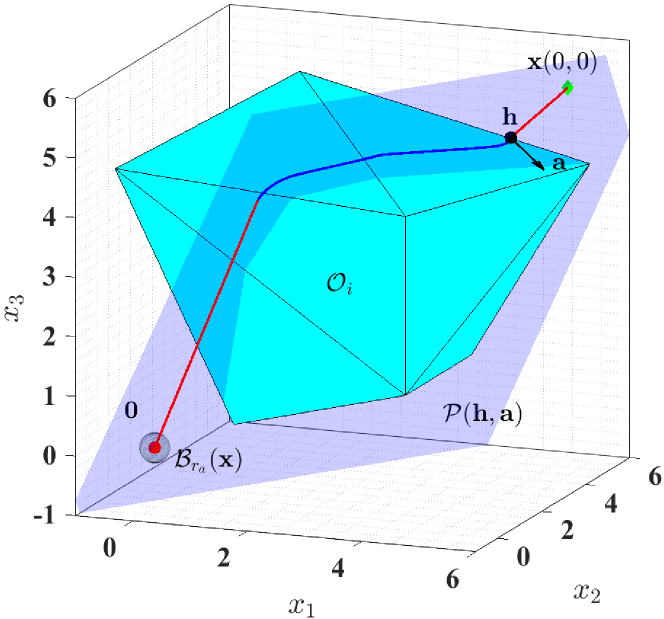
Figure 2: The trajectory of the robot safely converging to the target location at the origin.

We consider an unbounded workspace i.e., obstacle $\mathcal{O}_{0}=\emptyset$, with $2$ three-dimensional, convex obstacles, as shown in Fig. 3. We apply the proposed hybrid feedback controller (11) for robot initialized at $8$ different locations in the obstacle-free workspace. The target is located at the origin. The radius of the robot is set to $0.15m$. The minimum safety distance $r_{s}=0.05m$ and the parameter $\gamma=0.2m$. The gains $\kappa_{s}$ and $\kappa_{r}$, used in (11a), are set to $0.5$ and $1$, respectively. The sensing radius $R_{s}$, used in (32), is set to $1m$. The parameter $\epsilon$, used in (22), is set to 0.05m. From Fig. 3, it can be observed that the robot converges to the target location while simultaneously avoiding collisions with the obstacles. Fig. 4 shows that the center of the robot stays at least $r_{a}$ meters away from the boundary of the obstacles. The complete simulation video can be found at https://youtu.be/67eDVXH1wbw.

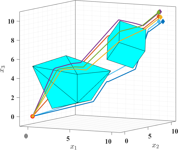
Figure 3: Robot trajectories starting from different locations.

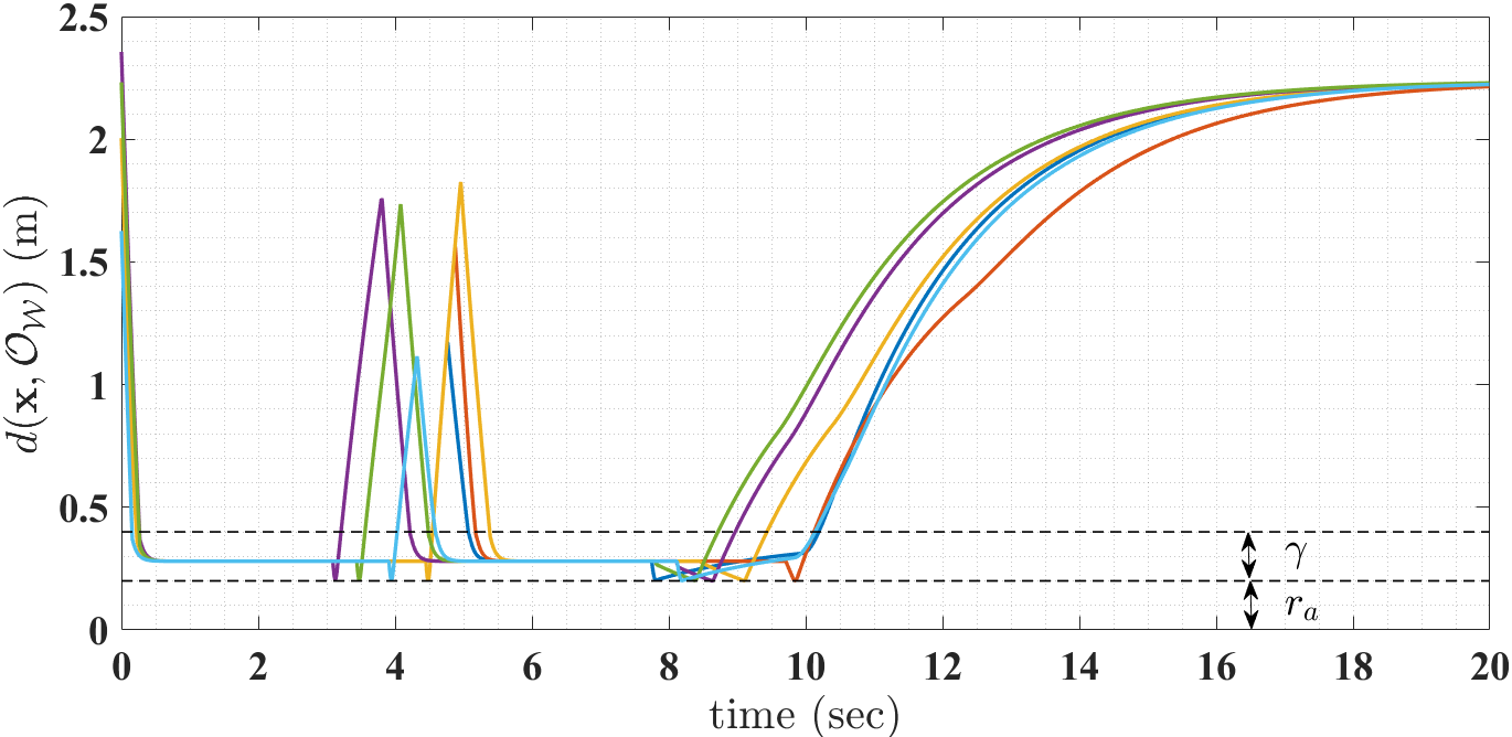
Figure 4: Distance of the center of the robot $\mathbf{x}$ from the boundary of the obstacle occupied workspace $\mathcal{O}_{\mathcal{W}}$.

VIII Conclusion

We propose a hybrid feedback controller for safe autonomous robot navigation in three-dimensional environments with arbitrarily-shaped convex obstacles. These obstacles may have nonsmooth boundaries, large sizes, and can be placed arbitrarily, provided they meet certain mild disjointedness requirements, as per Assumption 7. The proposed hybrid controller guarantees global asymptotic stability of the target location in the obstacle-free workspace. The obstacle-avoidance component of the control law relies on the projection of the robot’s center onto the nearest obstacle, enabling applications in a priori unknown environments, as discussed in Section VI. The proposed hybrid feedback control law generates discontinuous vector fields when switching between modes. Incorporating a smoothing mechanism in our proposed hybrid feedback would be an interesting practical extension. Moreover, extending our approach to second-order robot dynamics navigating in three-dimensional environments with non-convex obstacles, would be an interesting future work.

IX Appendix

IX-A Proof of Lemma 1

Since the target location at the origin $\mathbf{0}$ belongs to the interior of the obstacle-free workspace $\mathcal{W}_{r_{a}}^{\circ}$, there exists some distance between the target location and the $r_{a}-$dilated obstacle $\mathcal{D}_{r_{a}}(\mathcal{O}_{i})$. In other words, since $\mathbf{0}\in\mathcal{W}_{r_{a}}^{\circ},$ there exists $\bar{\delta}>0$ such that $d(\mathbf{0},\mathcal{D}_{r_{a}}(\mathcal{O}_{i}))=\bar{\delta}.$ Notice that, since the workspace satisfies Assumption 7, according to (18), the set $\mathcal{J}_{0}^{\mathcal{W}}\cap\mathcal{N}_{\gamma}(\mathcal{D}_{r_{a}}(\mathcal{O}_{i}))$ belongs to the landing region associated with obstacle $\mathcal{O}_{i}$ i.e., $\mathcal{J}_{0}^{\mathcal{W}}\cap\mathcal{N}_{\gamma}(\mathcal{D}_{r_{a}}(\mathcal{O}_{i}))\subset\mathcal{R}_{l}^{i}.$ According to (15), the location $\Pi(\mathbf{0},\mathcal{D}_{r_{a}}(\mathcal{O}_{i}))$ does not belong to the landing region $\mathcal{R}_{l}^{i}$. As a result, one has $d(\mathbf{0},\mathcal{R}_{l}^{i})>\bar{\delta}.$ Hence, it is clear that $\mathcal{B}_{\bar{\delta}}(\mathbf{0})\cap\mathcal{N}_{\gamma}(\mathcal{D}_{r_{a}}(\mathcal{O}_{i}))\cap\mathcal{J}_{0}^{\mathcal{W}}=\emptyset,$ where $\mathcal{B}_{\bar{\delta}}(\mathbf{0})\cap\mathcal{N}_{\gamma}(\mathcal{D}_{r_{a}}(\mathcal{O}_{i}))\neq\emptyset.$ Hence, one can set $\bar{\epsilon}\in(0,d(\mathbf{0},\mathcal{R}_{l}^{i})-\bar{\delta}]$ to ensure that $\mathcal{ER}^{\mathbf{h}}\cap\mathcal{N}_{\gamma}(\mathcal{D}_{r_{a}}(\mathcal{O}_{i}))\neq\emptyset$ for all $\mathbf{h}\in\mathcal{J}_{0}^{\mathcal{W}}\cap\mathcal{N}_{\gamma}(\mathcal{D}_{r_{a}}(\mathcal{O}_{i}))$, for any $\epsilon\in(0,\bar{\epsilon}].$

IX-B Proof of Lemma 2

The flow set $\mathcal{F}$ and the jump set $\mathcal{J}$, defined in (25) are by construction closed subsets of $\mathbb{R}^{3}\times\mathbb{R}^{3}\times\mathbb{R}^{3}\times\mathbb{R}\times\mathbb{R}.$ Hence, condition 1 in Lemma 2 is satisfied.

Since the flow map $\mathbf{F}(\xi)$ is defined for all $\xi\in\mathcal{F}$, $\mathcal{F}\subset\text{ dom }\mathbf{F}.$ The flow map $\mathbf{F},$ given in (30), is continuous on $\mathcal{F}_{0}.$ Next, we verify the continuity of $\mathbf{F}$ on $\mathcal{F}_{1}.$ Since $\gamma\in(0,\bar{r}_{s}-r_{s})$, the sets $\mathcal{N}_{\gamma}(\mathcal{D}_{r_{a}}(\mathcal{O}_{i}))$, for all $i\in\mathbb{I}$, are disjoint. Since obstacles $\mathcal{O}_{i},i\in\mathbb{I}\setminus\{0\}$ are convex, for all locations $\mathbf{x}\in\mathcal{N}_{\gamma}(\mathcal{D}_{r_{a}}(\mathcal{O}_{i})),i\in\mathbb{I}\setminus\{0\}$, the closest point from $\mathbf{x}$ on the boundary of the nearest obstacle $\Pi(\mathbf{x},\mathcal{O}_{i})$ is unique. Furthermore, according to (23), the set $\mathcal{F}_{1}^{\mathcal{W}}\subset\bigcup_{i\in\mathbb{I}\setminus\{0\}}\mathcal{N}_{\gamma}(\mathcal{D}_{r_{a}}(\mathcal{O}_{i}))$. Hence, according to [17] [Lemma 4.1] and (23), $\Pi(\mathbf{x},\mathcal{O}_{\mathcal{W}})$ is continuous for all $\mathbf{x}\in\mathcal{F}_{1}^{\mathcal{W}}$. Hence, the obstacle-avoidance control vector $\kappa_{r}\mathbf{v}(\mathbf{x},\mathbf{a})$, used in (11a), is continuous for all locations $\mathbf{x}\in\mathcal{F}_{1}^{\mathcal{W}}$ with the unit vector $\mathbf{a}$ chosen as per (27). As a result, $\mathbf{F}$ is continuous on $\mathcal{F}_{1}$ and as such it is continuous on $\mathcal{F}.$ This shows fulfillment of condition 2 in Lemma 2.

Since the jump map $\mathbf{J}(\xi)$ is defined for all $\xi\in\mathcal{J}$, $\mathcal{J}\subset\text{ dom }\mathbf{J}.$ The jump map $\mathbf{J}$, defined in (30), is single-valued on $\mathcal{J}_{1}$. Hence, according to [16, Definition 5.9 and 5.14], the jump map $\mathbf{J}$ is outer semicontinuous and locally bounded relative to $\mathcal{J}_{1}$. According to (27) and (30), the jump map $\mathbf{J}$ is single-valued for the state vector $(\mathbf{x},\mathbf{h},m,s)$ on $\mathcal{J}_{0}$. Consider the jump map $\mathbf{J}$ for the state $\mathbf{a}$ on $\mathcal{J}_{0}.$ We show that the set-valued mapping $\mathcal{P}^{\perp}:\mathbb{R}^{3}\rightrightarrows\mathbb{S}^{2}$, used in (27), is outer semicontinuous and locally bounded. To that end, consider any sequence $\{\mathbf{q}_{i}\}_{i\in\mathbb{N}}\subset\mathbb{R}^{3}$ that converges to $\mathbf{q}\in\mathbb{R}^{3}.$ Assume that the sequence $\{\mathbf{p}_{i}=\mathcal{P}^{\perp}(\mathbf{q}_{i})\}_{i\in\mathbb{N}}\subset\mathbb{S}^{2}$ converges to some $\mathbf{p}\in\mathbb{S}^{2}.$ Since, according to (28), the inner product $\mathbf{q}_{i}^{\top}\mathbf{p}_{i}=0$ for all $i\in\mathbb{N}$, the inner product $\mathbf{q}^{\top}\mathbf{p}=0.$ Consequently, $\mathbf{p}\in\mathcal{P}^{\perp}(\mathbf{q})$. Hence, according [16, Definition 5.9], the mapping $\mathcal{P}^{\perp}$ is outer semicontinuous. Since $\text{ rge }\mathcal{P}^{\perp}=\mathbb{S}^{2}\subset\mathbb{R}^{3}$ is bounded, according to [16, Definition 5.14], the set-valued mapping $\mathcal{P}^{\perp}$ is locally bounded, where the range of $\mathcal{P}^{\perp}$ is defined as per [16, Definition 5.8]. Hence, $\mathbf{J}$ is outer semi-continuous and locally bounded relative to $\mathcal{J}.$ This shows the fulfillment of condition 3 in Lemma 2.

IX-C Proof of Lemma 3

First we prove that the union of the flow and jump sets covers exactly the obstacle-free state space $\mathcal{K}$. For $m=0$, according to (18) and (19), by construction we have $\mathcal{F}_{0}^{\mathcal{W}}\cup\mathcal{J}_{0}^{\mathcal{W}}=\mathcal{W}_{r_{a}}.$ Similarly, for $m=1$, according to (21) and (23), by construction one has $\mathcal{F}_{m}^{\mathcal{W}}\cup\mathcal{J}_{m}^{\mathcal{W}}=\mathcal{W}_{r_{a}}$. Inspired by [12, Appendix 11], the satisfaction of the following equation:

$$\mathcal{F}_{m}^{\mathcal{W}}\cup\mathcal{J}_{m}^{\mathcal{W}}=\mathcal{W}_{r_{a}},m\in\mathbb{M},$$ (34)

along with (20), (24) and (25) implies $\mathcal{F}\cup\mathcal{J}=\mathcal{K}.$

Now, inspired by [12, Appendix 1], for the hybrid closed-loop system (30), with data $\mathcal{H}=(\mathcal{F},\mathbf{F},\mathcal{J},\mathbf{J}),$ define $\mathbf{S}_{\mathcal{H}}(\mathcal{K})$ as the set of all maximal solutions $\xi$ to $\mathcal{H}$ with $\xi(0,0)\in\mathcal{K}$. Since $\mathcal{F}\cup\mathcal{J}=\mathcal{K}$, each $\xi\in\mathbf{S}_{\mathcal{H}}(\mathcal{K})$ has range $\text{rge }\xi\subset\mathcal{K}.$ Additionally, if every maximal solution $\xi\in\mathbf{S}_{\mathcal{H}}(\mathcal{K})$ is complete, then the set $\mathcal{K}$ will be forward invariant [18, Definition 3.13]. Since the hybrid closed-loop system (30) satisfies the hybrid basic conditions, as stated in Lemma 2, one can use [16, Proposition 6.10], to verify the following viability condition:

$$\mathbf{F}(\xi)\cap\mathbf{T}_{\mathcal{F}}(\xi)\neq\emptyset,\forall\xi\in\mathcal{F}\setminus\mathcal{J},$$ (35)

which will allow us to establish the completeness of the solution $\xi$ to the hybrid closed-loop system (30). In (35), $\mathbf{T}_{\mathcal{F}}(\xi)$ represents the tangent cone to the set $\mathcal{F}$ at $\xi$.

Let $(\mathbf{x},\mathbf{h},\mathbf{a},m,s)\in\mathcal{F}\setminus\mathcal{J}$, which implies by (20), (24) and (25) that $(\mathbf{x},\mathbf{h},\mathbf{a},s)\in(\mathcal{F}_{m}^{\mathcal{W}}\setminus\mathcal{J}_{m}^{\mathcal{W}})\times\mathcal{W}_{r_{a}}\times\mathbb{S}^{2}\times\mathbb{R}_{\geq 0}$ for some $m\in\mathbb{M}$. For $\mathbf{x}\in(\mathcal{F}_{m}^{\mathcal{W}})^{\circ}\setminus\mathcal{J}_{m}^{\mathcal{W}}$ with $(\mathbf{h},\mathbf{a},m,s)\in\mathcal{W}_{r_{a}}\times\mathbb{S}^{2}\times\mathbb{M}\times\mathbb{R}_{\geq 0}$ the tangent cone $\mathbf{T}_{\mathcal{F}}(\xi)=\mathbb{R}^{3}\times\mathbf{T}_{\mathcal{W}_{r_{a}}}(\mathbf{h})\times\mathcal{P}(\mathbf{0},\mathbf{a})\times\{0\}\times\mathbf{T}_{\mathbb{R}_{\geq 0}}(s),$ where the set $\mathbf{T}_{\mathcal{W}_{r_{a}}}(\mathbf{h})$ is given by

$${\mathbf{T}_{\mathcal{W}_{r_{a}}}(\mathbf{h})}=\begin{cases}\begin{matrix}[l]\mathbb{R}^{3},&\text{if }\mathbf{h}\in(\mathcal{W}_{r_{a}})^{\circ},\\ \mathcal{P}_{\geq}(\mathbf{0},(\mathbf{h}-\Pi(\mathbf{h},\mathcal{O}_{\mathcal{W}}))),&\text{if }\mathbf{h}\in\partial\mathcal{W}_{r_{a}},\end{matrix}\end{cases}$$ (36)

where for $\mathbf{h}\in\partial\mathcal{W}_{r_{a}}$, the projection $\Pi(\mathbf{h},\mathcal{O}_{\mathcal{W}})$ is unique. For $s\in\mathbb{R}_{\geq 0}$, the set $\mathbf{T}_{\mathbb{R}_{\geq 0}}(s)$ is defined as

$${\mathbf{T}_{\mathbb{R}_{\geq 0}}(s)}=\begin{cases}\begin{matrix}[l]\mathbb{R},&\text{if }s\in\mathbb{R}_{>0},\\ \mathbb{R}_{\geq 0},&\text{if }s=0.\end{matrix}\end{cases}$$ (37)

Since, according to (30), $\dot{\mathbf{h}}=\mathbf{0}$ and $\dot{s}=1$, we have $\dot{\mathbf{h}}\in\mathbf{T}_{\mathcal{W}_{r_{a}}}(\mathbf{h})$ and $\dot{s}\in\mathbf{T}_{\mathbb{R}_{\geq 0}}(s)$, respectively, and (35) holds.

For $m=0$, according to (18) and (19), one has

$$\partial\mathcal{F}_{0}^{\mathcal{W}}\setminus\mathcal{J}_{0}^{\mathcal{W}}\subset\partial\mathcal{D}_{r_{a}}(\mathcal{O}_{\mathcal{W}})\cap\mathcal{R}_{e},$$ (38)

and for $\mathbf{x}\in\partial\mathcal{F}_{0}^{\mathcal{W}}\setminus\mathcal{J}_{0}^{\mathcal{W}},$ the projection $\Pi(\mathbf{x},\mathcal{O}_{\mathcal{W}})$ is unique. Hence, $\forall\mathbf{x}\in\partial\mathcal{F}_{0}^{\mathcal{W}}\setminus\mathcal{J}_{0}^{\mathcal{W}}$,

$$\mathbf{T}_{\mathcal{F}}(\xi)=\mathcal{P}_{\geq}(\mathbf{0},\mathbf{x}_{\pi})\times\mathbf{T}_{\mathcal{W}_{r_{a}}}(\mathbf{h})\times\mathcal{P}(\mathbf{0},\mathbf{a})\times\{0\}\times\mathbf{T}_{\mathbb{R}_{\geq 0}}(s),$$ (39)

where $\mathbf{T}_{\mathcal{W}_{r_{a}}}(\mathbf{h})$ and $\mathbf{T}_{\mathbb{R}_{\geq 0}}(s)$ are defined in (36) and (37), respectively, and $\mathbf{x}_{\pi}=\mathbf{x}-\Pi(\mathbf{x},\mathcal{O}_{\mathcal{W}})$. Also, according to (11a), for $m=0$, one has $\mathbf{u}(\xi)=-\kappa_{s}\mathbf{x},\kappa_{s}>0$. According to (17) and (38), for $\xi\in\mathcal{F}_{0}\setminus\mathcal{J}_{0}$ with $\mathbf{x}\in\partial\mathcal{F}_{0}^{\mathcal{W}}\setminus\mathcal{J}_{0}^{\mathcal{W}}$, one can conclude that $\mathbf{u}(\xi)\in\mathcal{P}_{\geq}(\mathbf{0},\mathbf{x}_{\pi})$. Moreover, according to (30), it is clear that $\dot{\mathbf{h}}=\mathbf{0}\in\mathbf{T}_{\mathcal{W}_{r_{a}}}(\mathbf{h})$, $\dot{s}=1\in\mathbf{T}_{\mathbb{R}_{\geq 0}}(s)$ and $\dot{\mathbf{a}}=0\in\mathcal{P}(\mathbf{0},\mathbf{a})$. Therefore, the viability condition (35) holds for $m=0$.

For $m=1$, according to (21) and (23) one has

$$\partial\mathcal{F}_{1}^{\mathcal{W}}\setminus\mathcal{J}_{1}^{\mathcal{W}}\subset\partial\mathcal{D}_{r_{a}}(\mathcal{O}_{\mathcal{W}}),$$ (40)

and for $\mathbf{x}\in\partial\mathcal{F}_{1}^{\mathcal{W}}\setminus\mathcal{J}_{1}^{\mathcal{W}}$, the projection $\Pi(\mathbf{x},\mathcal{O}_{\mathcal{W}})$ is unique and the circle $\mathcal{B}_{\lVert\mathbf{x}_{\pi}\rVert}(\mathbf{x})$ intersect with $\partial\mathcal{O}_{\mathcal{W}}$ only at the location $\Pi(\mathbf{x},\mathcal{O}_{\mathcal{W}}).$ Hence, $\forall\mathbf{x}\in\partial\mathcal{F}_{1}^{\mathcal{W}}\setminus\mathcal{J}_{1}^{\mathcal{W}}$, the tangent cone

$$\mathbf{T}_{\mathcal{F}}(\xi)=\mathcal{P}_{\geq}(\mathbf{0},\mathbf{x}_{\pi})\times\mathbf{T}_{\mathcal{W}_{r_{a}}}(\mathbf{h})\times\mathcal{P}(\mathbf{0},\mathbf{a})\times\{0\}\times\mathbf{T}_{\mathbb{R}_{\geq 0}}(s),$$ (41)

where $\mathbf{T}_{\mathcal{W}_{r_{a}}}(\mathbf{h})$ and $\mathbf{T}_{\mathbb{R}_{\geq 0}}(s)$ are defined in (36) and (37), respectively. Also, according to (11a), for $m=1$, one has $\mathbf{u}(\xi)=\kappa_{r}\mathbf{v}(\mathbf{x},\mathbf{a}),\kappa_{r}>0.$ From (14), it follows that $\eta(\mathbf{x})=1$ for $\mathbf{x}\in\partial\mathcal{F}_{1}^{\mathcal{W}}\setminus\mathcal{J}_{1}^{\mathcal{W}}$. As a result, according to (11a) and (12), the control vector is simplified to $\mathbf{u}(\xi)=\kappa_{r}{\mathbf{P}(\mathbf{a})\mathbf{x}_{\pi}}.$ It can be shown that for any $\mathbf{a}\in\mathbb{S}^{2}$, the inner product $\mathbf{x}_{\pi}^{\intercal}\mathbf{P}(\mathbf{a})\mathbf{x}_{\pi}$ is always non-negative. Therefore, for $\xi\in\mathcal{F}_{1}\setminus\mathcal{J}_{1}$ with $\mathbf{x}\in\mathcal{F}_{1}^{\mathcal{W}}\setminus\mathcal{J}_{1}^{\mathcal{W}}$, one has $\mathbf{u}(\mathbf{x},\mathbf{h},\mathbf{a},1,s)^{\intercal}(\mathbf{x}-\Pi(\mathbf{x},\mathcal{O}_{\mathcal{W}}))\geq 0$. Moreover, according to (30), it is clear that $\dot{\mathbf{h}}=\mathbf{0}\in\mathbf{T}_{\mathcal{W}_{r_{a}}}(\mathbf{h})$, $\dot{s}=1$ and $\dot{\mathbf{a}}=0\in\mathcal{P}(\mathbf{0},\mathbf{a})$. Hence, the viability condition in (35) holds for $m=1.$

Hence, according to [16, Proposition 6.10], since (35) holds for all $\xi\in\mathcal{F}\setminus\mathcal{J}$, there exists a nontrivial solution to $\mathcal{H}$ for each initial condition in $\mathcal{K}$. Finite escape time can only occur through flow. They can neither occur for $\mathbf{x}$ in the set $\mathcal{F}_{1}^{\mathcal{W}}$, as this set is bounded as per definition (23), nor for $\mathbf{x}$ in the set $\mathcal{F}_{0}^{\mathcal{W}}$ as this would make $\mathbf{x}^{\intercal}\mathbf{x}$ grow unbounded, and would contradict the fact that $\frac{d}{dt}(\mathbf{x}^{\intercal}\mathbf{x})\leq 0$ in view of the definition of $\mathbf{u}(\mathbf{x},\mathbf{h},\mathbf{a},0,s)$. Therefore, all maximal solutions do not have finite escape times. Furthermore, according to (30), $\mathbf{x}^{+}=\mathbf{x},$ and from the definition of the update law in (27) and (29), it follows immediately that $\mathbf{J}(\mathcal{J})\subset\mathcal{K}$. Hence, the solutions to the hybrid closed-loop system (30) cannot leave $\mathcal{K}$ through jump and, as per [16, Proposition 6.10], all maximal solutions are complete.

IX-D Proof of Theorem 1

Forward invariance and stability: The forward invariance of the obstacle-free set $\mathcal{K}$, for the hybrid closed-loop system (30), is immediate from Lemma 3. We next prove the stability of $\mathcal{A}$ using [16, Definition 7.1].

Since $\mathbf{0}\in(\mathcal{W}_{r_{a}})^{\circ}$, there exists $\mu_{1}>0$ such that $\mathcal{B}_{\mu_{1}}(\mathbf{0})\cap(\mathcal{D}_{r_{a}}(\mathcal{O}_{\mathcal{W}}))^{\circ}=\emptyset.$ According to (18), there exists $\mu_{2}>0$ such that $\mathcal{B}_{\mu_{2}}(\mathbf{0})\cap\mathcal{J}_{0}^{\mathcal{W}}=\emptyset$. We define the set $\mathcal{S}_{\mu}:=\{\xi\in\mathcal{K}|\mathbf{x}\in\mathcal{B}_{\mu}(\mathbf{0})\},$ where $\mu\in(0,\min\{\mu_{1},\mu_{2}\}).$ Notice that for all initial conditions $\xi(0,0)\in\mathcal{S}_{\mu}$, the control input, after at most one jump corresponds to the move-to-target mode and it steers the state $\mathbf{x}$ towards the origin according to the control input vector $\mathbf{u}(\xi)=-\kappa_{s}\mathbf{x},\kappa_{s}>0$. Hence, for each $\mu\in(0,\min\{\mu_{1},\mu_{2}\}),$ the set $\mathcal{S}_{\mu}$ is forward invariant for the hybrid closed-loop system (30).

Consequently, for every $\rho>0$, one can choose $\sigma\in(0,\min\{\mu_{1},\mu_{2},\rho\})$ such that for all initial conditions $\xi(0,0)$ with $d(\xi(0,0),\mathcal{A})\leq\sigma$, one has $d(\xi(t,j),\mathcal{A})\leq\rho$ for all $(t,j)\in\text{ dom }\xi,$ where $d(\xi,\mathcal{A})^{2}=\underset{(\mathbf{0},\bar{\mathbf{h}},\bar{\mathbf{a}},\bar{m},s)\in\mathcal{A}}{\inf}(\lVert\mathbf{x}\rVert^{2}+\lVert\mathbf{h}-\bar{\mathbf{h}}\rVert^{2}+\lVert\mathbf{a}-\bar{\mathbf{a}}\rVert^{2}+(m-\bar{m})^{2}+(s-\bar{s})^{2})=\lVert\mathbf{x}\rVert^{2}.$ Hence, according to [18, Definition 3.1], the target set $\mathcal{A}$ is stable for the hybrid closed-loop system (30). Next, we proceed to establish the convergence properties of the set $\mathcal{A}$.

Attractivity: We aim to show that for the proposed hybrid closed-loop system (30), the target set $\mathcal{A}$ is globally attractive in the set $\mathcal{K}$ using [18, Defintion 3.1 and Remark 3.5]. In other words, we prove that for all initial conditions $\xi(0,0)\in\overline{\mathcal{F}}\cup\mathcal{J}=\mathcal{K}$, every maximal solution $\xi$ to the hybrid closed-loop system is complete and satisfies

$$\underset{(t,j)\in\text{ dom }\xi,t+j\to\infty}{\lim}d(\xi(t,j),\mathcal{A})=\lVert\mathbf{x}(t,j)\rVert=0.$$ (42)

The completeness of all maximal solutions to the hybrid closed-loop system (30) follows from Lemma 3. Next, we prove that for all initial condition $\xi(0,0)\in\mathcal{K}$, every complete solution $\xi$ to the hybrid closed-loop system (30), satisfies (42). We consider two cases based on the initial value of the mode indicator variable $m(0,0)$.

Case 1: $m(0,0)=0$. For the hybrid closed-loop system (30), consider a solution $\xi$ initialized in the move-to-target mode. Let us assume $\xi(t_{0},j_{0})\in\mathcal{F}_{0}$ for some $(t_{0},j_{0})\in\text{ dom }\xi,(t_{0},j_{0})\succeq(0,0).$ If $\xi(t,j)\notin\mathcal{J}_{0}$, for all $(t,j)\succeq(t_{0},j_{0})$, then the control input $\mathbf{u}(\mathbf{x},\mathbf{h},\mathbf{a},0,s)=-\kappa_{s}\mathbf{x}$ will steer the state $\mathbf{x}$ straight towards the origin, where $\kappa_{s}>0$. On the other hand, assume that there exists $(t_{1},j_{1})\succeq(t_{0},j_{0})$ such that $\xi(t_{1},j_{1})\in\mathcal{J}_{0}$. Then, according to (27), the control law switches to the obstacle-avoidance mode. As per (18), it is clear that $\mathbf{x}(t_{1},j_{1})\in\mathcal{J}_{0}^{\mathcal{W}}\cap\mathcal{N}_{\gamma_{s}}(\mathcal{D}_{r_{a}}(\mathcal{O}_{i})),$ for some $i\in\mathbb{I}$ and $d(\mathbf{x}(t_{1},j_{1}),\mathcal{O}_{i})=\beta$ for some $\beta\in[r_{a},r_{a}+\gamma_{s}].$ At this instance, according to (27), the proposed navigation algorithm updates the values of the state variable $\mathbf{h}(t_{1},j_{1}+1)=\mathbf{x}(t_{1},j_{1})$, $\mathbf{a}(t_{1},j_{1}+1)\in\mathcal{P}^{\perp}(\mathbf{x}(t_{1},j_{1}))$, $m(t_{1},j_{1}+1)=1$ and $s(t_{1},j_{1}+1)=s(t_{1},j_{1})+1.$ To proceed with the proof, we need the following lemma:

Lemma 4.

Under Assumption 7, consider a solution $\xi$ to the hybrid closed-loop system (30). If $\xi(t_{1},j_{1})\in\mathcal{J}_{0}$ at some $(t_{1},j_{1})\in\text{ dom }\xi$ such that $\mathbf{x}(t_{1},j_{1})\in\mathcal{J}_{0}^{\mathcal{W}}\cap\mathcal{N}_{\gamma}(\mathcal{D}_{r_{a}}(\mathcal{O}_{i}))$ for some $i\in\mathbb{I}$, then for all $(t,j)\in(I_{j_{1}+1}\times j_{1}+1)$, where $I_{j_{1}+1}=\{t|(t,j_{1}+1)\in\text{ dom }\xi\}$, the following statements hold true:

1. the inner product $\mathbf{x}_{\pi}(t,j)^{\intercal}\mathbf{P}(\mathbf{a}(t,j))\mathbf{x}_{\pi}(t,j)>0$, where $\mathbf{x}_{\pi}(t,j)=\mathbf{x}(t,j)-\Pi(\mathbf{x}(t,j),\mathcal{O}_{\mathcal{W}})$,

2. the state $\mathbf{x}(t,j)\in\mathcal{P}(\mathbf{h}(t_{1},j_{1}+1),\mathbf{a}(t_{1},j_{1}+1))\cap\mathcal{N}_{\gamma}(\mathcal{D}_{r_{a}}(\mathcal{O}_{i}))$,

3. there exists $t_{2}>t_{1}$ such that $t_{2}<\infty$ and $\xi(t_{2},j_{1}+1)\in\mathcal{J}_{1}.$

Proof.

See Appendix IX-E. ∎

According to Lemma 4, when a solution $\xi$ to the hybrid closed-loop system (30) evolves in the obstacle-avoidance mode, the state $\xi$ eventually enters in the jump set of the obstacle-avoidance mode $\mathcal{J}_{1}$ (24) and the control law switches to the move-to-target mode.

According to Lemma 4, there exists $(t_{2},j_{1}+1)\succ(t_{1},j_{1}+1)$ with $t_{2}<\infty$ such that $\xi(t_{2},j_{1}+1)\in\mathcal{J}_{1}$. Notice that, according to (21) and (22), one has $\|\mathbf{x}(t_{2},j_{1}+1)\|<\|\mathbf{x}(t_{1},j_{1}+1)\|$. In other words, according to Lemma 4, the proposed navigation algorithm ensures that, at the instance where the the control switches from the obstacle-avoidance mode to the move-to-target mode, the origin is closer to the point $\mathbf{x}$ than to the last point where the control switched to the obstacle-avoidance mode. Furthermore, when the control input corresponds to the move-to-target mode, it steers the state $\mathbf{x}$ towards the origin under the influence of control $\mathbf{u}(\xi)=-\kappa_{s}\mathbf{x},\kappa_{s}>0.$ Consequently, given that the workspace $\mathcal{W}$ and the obstacles $\mathcal{O}_{i},i\in\mathbb{I}\setminus\{0\}$, are compact, it can be concluded that the solution $\xi(t,j)$ will contain finite number of jumps and will satisfy (42).

Case 2: $m(0,0)=1.$ For the hybrid closed-loop system (30) consider a solution $\xi$ initialized in the obstacle-avoidance mode. Since $m(0,0)=1$, according to (24), $\xi(0,0)\in\mathcal{J}_{1}$. Therefore, according to (29), the control input switches to the move-to-target mode and $m(0,1)=0.$ One can now use arguments similar to the ones used for case 1 to show that the solution $\xi(t,j)$ will contain finite number of jumps and will satisfy (42).

Hence, the target set $\mathcal{A}$ is globally attractive in the set $\mathcal{K}$ for the proposed hybrid closed-loop system (30). In addition, since the set $\mathcal{A}$ is stable for the hybrid closed-loop system (30), it is globally asymptotically stable in the set $\mathcal{K}$ for the hybrid closed-loop system (30) as per [18, Remark 3.5].

IX-E Proof of Lemma 4

When the state $\xi$ enters in the jump set of the move-to-target mode $\mathcal{J}_{0}$ (20), the control law switches to the obstacle-avoidance mode by updating the mode indicator variable $m(t_{1},j_{1}+1)$ to $1$, using (27). Hence, for all time $(t,j)\in({I_{j_{1}+1}}\times j_{1}+1)$, the control vector $\mathbf{u}(\xi(t,j))$ in (11a) is given by

$$\mathbf{u}(t,j)=\kappa_{r}\mathbf{v}(\mathbf{x}(t,j),\mathbf{a}(t,j)),$$ (43)

where $\mathbf{a}(t,j)=\mathbf{a}(t_{1},j_{1}+1)$ as per (27). Observe that for all $(t,j)\in({I_{j_{1}+1}}\times j_{1}+1)$, one has $\mathbf{v}(\mathbf{x}(t,j),\mathbf{a}(t,j))\in\mathcal{P}(\mathbf{x}(t_{1},j_{1}+1),\mathbf{a}(t_{1},j_{1}+1))$ and, according to (27), $\mathbf{h}(t_{1},j_{1}+1)=$ $\mathbf{x}(t_{1},j_{1}+1)$. Hence, for all $(t,j)\in({I_{j_{1}+1}}\times j_{1}+1)$,

$$\mathbf{x}(t,j)\in\mathcal{P}(\mathbf{h}(t_{1},j_{1}+1),\mathbf{a}(t_{1},j_{1}+1)).$$ (44)

Since $\mathbf{x}(t_{1},j_{1})\in\mathcal{J}_{0}^{\mathcal{W}}\cap\mathcal{N}_{\gamma_{s}}(\mathcal{D}_{r_{a}}(\mathcal{O}_{i}))$ and $\mathbf{a}(t_{1},j_{1}+1)\in\mathcal{P}^{\perp}(\mathbf{x}(t_{1},j_{1}))$, the hyperplane $\mathcal{P}(\mathbf{h}(t_{1},j_{1}+1),\mathbf{a}(t_{1},j_{1}+1))$ has a non-empty intersection with the interior of the $r_{a}-$dilated obstacle $\mathcal{D}_{r_{a}}(\mathcal{O}_{i})$ i.e., $\mathcal{P}(\mathbf{h}(t_{1},j_{1}+1),\mathbf{a}(t_{1},j_{1}+1))\cap\mathcal{D}_{r_{a}}^{\circ}(\mathcal{O}_{i})\neq\emptyset.$ As a result, it can be shown that there does not exist a point $\mathbf{q}$ in the set $\mathcal{P}(\mathbf{h}(t_{1},j_{1}+1),\mathbf{a}(t_{1},j_{1}+1))\setminus\mathcal{D}_{r_{a}}^{\circ}(\mathcal{O}_{i})$ such that the vector $\mathbf{P}(\mathbf{a}(t_{1},j_{1}+1))(\mathbf{q}-\Pi(\mathbf{q},\mathcal{O}_{i}))=\mathbf{0}.$ Moreover, for any non-zero vectors $\mathbf{z}\in\mathbb{R}^{3}\setminus\{\mathbf{0}\}$ and $\mathbf{s}\in\mathbb{R}^{3}\setminus\{\mathbf{0}\}$, the inner product $\mathbf{z}^{\intercal}\mathbf{P}(\mathbf{s})\mathbf{z}$ is always non-negative and is zero only if $\mathbf{P}(\mathbf{a})\mathbf{z}=0.$ Since $\mathbf{x}(t,j)\in\mathcal{P}(\mathbf{h}(t_{1},j_{1}+1),\mathbf{a}(t_{1},j_{1}+1))$ and $\mathbf{a}(t,j)=\mathbf{a}(t_{1},j_{1}+1)$ for all $(t,j)\in({I_{j_{1}+1}}\times j_{1}+1)$, one has $\mathbf{x}_{\pi}(t,j)^{\intercal}\mathbf{P}(\mathbf{a}(t,j))\mathbf{x}_{\pi}(t,j)>0$, where $\mathbf{x}_{\pi}(t,j)=\mathbf{x}(t,j)-\Pi(\mathbf{x}(t,j),\mathcal{O}_{\mathcal{W}}),$ with $\Pi(\mathbf{x}(t,j),\mathcal{O}_{\mathcal{W}})=\Pi(\mathbf{x}(t,j),\mathcal{O}_{i}),$ and claim 1 in Lemma 4 is proved.

Next, we shows that when the control input corresponds to the obstacle-avoidance mode,

$$\mathbf{u}(\xi)\in\mathbf{T}_{\mathcal{N}_{\gamma}(\mathcal{D}_{r_{a}}(\mathcal{O}_{i}))}(\mathbf{x}),$$ (45)

for all $\mathbf{x}\in\mathcal{P}(\mathbf{h}(t_{1},j_{1}+1),\mathbf{a}(t_{1},j_{1}+1))\cap\partial\mathcal{N}_{\gamma}(\mathcal{D}_{r_{a}}(\mathcal{O}_{i}))$. This, combined with the facts that the control vector trajectory $\mathbf{u}(\xi)$ is continuous, when it corresponds to the obstacle-avoidance mode, according to Lemma 2, ensures that $\mathbf{x}(t,j)\in\mathcal{N}_{\gamma}(\mathcal{D}_{r_{a}}(\mathcal{O}_{i}))$ for all $(t,j)\in(I_{j_{1}+1}\times j_{1}+1)$.

Note that $\partial\mathcal{N}_{\gamma}(\mathcal{D}_{r_{a}}(\mathcal{O}_{i}))=\partial\mathcal{D}_{r_{a}}(\mathcal{O}_{i})\cup\partial\mathcal{D}_{r_{a}+\gamma}(\mathcal{O}_{i}).$ We know that for all $\mathbf{x}\in\partial\mathcal{D}_{r_{a}}(\mathcal{O}_{i})$, one has $\mathcal{P}_{\geq}(\mathbf{0},\mathbf{x}_{\pi})\subseteq\mathbf{T}_{\mathcal{N}_{\gamma}(\mathcal{D}_{r_{a}}(\mathcal{O}_{i}))}(\mathbf{x})$, where $\mathbf{x}_{\pi}=\mathbf{x}-\Pi(\mathbf{x},\mathcal{O}_{\mathcal{W}})$ with $\Pi(\mathbf{x},\mathcal{O}_{\mathcal{W}})=\Pi(\mathbf{x},\mathcal{O}_{i}).$ Also, since the control input corresponds to the obstacle-avoidance mode, for $\mathbf{x}\in\partial\mathcal{D}_{r_{a}}(\mathcal{O}_{i})\cap\mathcal{P}(\mathbf{h}(t_{1},j_{1}+1),\mathbf{a}(t_{1},j_{1}+1))$, the control vector (11a) is given by $\mathbf{u}(\xi)=\kappa_{r}{\mathbf{P}(\mathbf{a}(t_{1},j_{1}+1))\mathbf{x}_{\pi}}$. Moreover, according to claim 1 in Lemma 4, one has $\mathbf{x}_{\pi}^{\intercal}\mathbf{P}(\mathbf{a}(t_{1},j_{1}+1))\mathbf{x}_{\pi}>0$. Hence, the control vector $\mathbf{u}(\xi)$ belongs to the open half-space $\mathcal{P}_{>}(\mathbf{h}(t_{1},j_{1}+1),\mathbf{a}(t_{1},j_{1}+1))$. As a result, in this case, for all $\mathbf{x}\in\mathcal{P}(\mathbf{h}(t_{1},j_{1}+1),\mathbf{a}(t_{1},j_{1}+1))\cap\partial\mathcal{D}_{r_{a}}(\mathcal{O}_{i})$, condition (45) holds true.

It is clear that for all $\mathbf{x}\in\partial\mathcal{D}_{r_{a}+\gamma}(\mathcal{O}_{i})$, one has $\mathcal{P}_{\leq}(\mathbf{0},\mathbf{x}_{\pi})\subseteq\mathbf{T}_{\mathcal{N}_{\gamma}(\mathcal{D}_{r_{a}}(\mathcal{O}_{i}))}(\mathbf{x})$. Also, since the control input corresponds to the obstacle-avoidance mode, for $\mathbf{x}\in\partial\mathcal{D}_{r_{a}+\gamma}(\mathcal{O}_{i})\cap\mathcal{P}(\mathbf{h}(t_{1},j_{1}+1),\mathbf{a}(t_{1},j_{1}+1))$, the control vector (11a) is given by $\mathbf{u}(\xi)=-\kappa_{r}{\mathbf{P}(\mathbf{a}(t_{1},j_{1}+1))\mathbf{x}_{\pi}}$ . Moreover, according to claim 1 in Lemma 4, it is clear that $\mathbf{x}_{\pi}^{\intercal}\mathbf{P}(\mathbf{a}(t_{1},j_{1}+1))\mathbf{x}_{\pi}>0$. Hence, the control vector $\mathbf{u}(\xi)$ belongs to the open half-space $\mathcal{P}_{<}(\mathbf{h}(t_{1},j_{1}+1),\mathbf{a}(t_{1},j_{1}+1))$. As a result, in this case, for all $\mathbf{x}\in\mathcal{P}(\mathbf{h}(t_{1},j_{1}+1),\mathbf{a}(t_{1},j_{1}+1))\cap\partial\mathcal{D}_{r_{a}+\gamma}(\mathcal{O}_{i})$, condition (45) holds true. Hence, using (44) and (45), claim 2 in Lemma 4 is proved.

Next, we proceed to prove claim 3 in Lemma 4 which implies that when $\xi(t_{1},j_{1}+1)\in\mathcal{F}_{1}$ for some $(t_{1},j_{1}+1)\in\text{ dom }\xi$, the control input steers the state $\xi$ to the jump set of the obstacle-avoidance mode $\mathcal{J}_{1}$ in finite time $(t_{2},j_{1}+1)\succ(t_{1},j_{1}+1)$ with $t_{2}<\infty.$

Let us define the set $\mathcal{O}_{i}^{\mathcal{S}}=\mathcal{D}_{r_{a}}(\mathcal{O}_{i})\cap\mathcal{P}(\mathbf{h}(t_{1},j_{1}+1),\mathbf{a}(t_{1},j_{1}+1))$, as shown in Fig. 5. Since obstacle $\mathcal{O}_{i}$ is convex, the set $\mathcal{O}_{i}^{\mathcal{S}}$ is also convex. As a result, the target location has a unique closest point on the set $\mathcal{O}_{i}^{\mathcal{S}}$, represented by $\Pi(\mathbf{0},\mathcal{O}_{i}^{\mathcal{S}}).$ Let us define the set $\mathcal{LS}:=\mathcal{L}_{s}(\mathbf{0},\Pi(\mathbf{0},\mathcal{O}_{i}^{\mathcal{S}}))\cap\mathcal{N}_{\gamma}(\mathcal{D}_{r_{a}}(\mathcal{O}_{i}))$. Since $\mathbf{0}\in\mathcal{P}(\mathbf{h}(t_{1},j_{1}+1),\mathbf{a}(t_{1},j_{1}+1)),$ the line segment $\mathcal{LS}$ belongs to the hyperplane $\mathcal{P}(\mathbf{h}(t_{1},j_{1}+1),\mathbf{a}(t_{1},j_{1}+1)).$ Note that the line segment $\mathcal{LS}$ also belongs to the exit region $\mathcal{R}_{e}$. Since the hit point $\mathbf{h}(t_{1},j_{1}+1)$ belongs to $\mathcal{R}_{l}^{i}$, the target location $\mathbf{0}$ is closer to the location $\Pi(\mathbf{0},\mathcal{O}_{i}^{\mathcal{S}})$ than to the hit point $\mathbf{h}(t_{1},j_{1}+1)$. Hence, for a sufficiently small value of $\bar{\epsilon}$, used in (22), one can ensure that the set $\mathcal{LS}$ belongs to the set $\mathcal{J}_{1}^{\mathcal{W}}$.

Now, if one ensures that the state $\mathbf{x}$, which belongs to the set $\mathcal{N}_{\gamma}(\mathcal{D}_{r_{a}}(\mathcal{O}_{i}))\cap\mathcal{P}(\mathbf{h}(t_{1},j_{1}+1),\mathbf{a}(t_{1},j_{1}+1))$ after time $(t_{1},j_{1})$, in the obstacle-avoidance mode around obstacle $\mathcal{O}_{i}$, eventually intersects the set $\mathcal{LS}$ at some finite time $(t_{2},j_{1}+1)\succ(t_{1},j_{1}+1)$, then it will imply that $\xi(t_{2},j_{1}+1)\in\mathcal{J}_{1}$, and claim 3 in Lemma 4 will be proven. To that end, let us divide the set $\mathcal{N}_{\gamma}(\mathcal{D}_{r_{a}}(\mathcal{O}_{i}))\cap\mathcal{P}(\mathbf{h}(t_{1},j_{1}+1),\mathbf{a}(t_{1},j_{1}+1))$, as shown in Fig. 5, into 3 separate subsets as follows:

$$\mathcal{N}_{\gamma}(\mathcal{D}_{r_{a}}(\mathcal{O}_{i}))\cap\mathcal{P}(\mathbf{h},\mathbf{a})=\mathcal{S}_{1}\cup\mathcal{S}_{2}\cup\mathcal{S}_{3},$$ (46)

where $\mathbf{h}=\mathbf{h}(t_{1},j_{1}+1),\mathbf{a}=\mathbf{a}(t_{1},j_{1}+1)$, and the sets $\mathcal{S}_{1},\mathcal{S}_{2}$ and $\mathcal{S}_{3}$ are defined as follows:

$$\mathcal{S}_{1}=\mathcal{N}_{\gamma_{a}}(\mathcal{D}_{r_{a}}(\mathcal{O}_{i}))\cap\mathcal{P}(\mathbf{h},\mathbf{a}),$$ (47)

$$\mathcal{S}_{2}=\mathcal{N}_{\gamma_{s}-\gamma_{a}}^{\circ}(\mathcal{D}_{r_{a}+\gamma_{a}}(\mathcal{O}_{i}))\cap\mathcal{P}(\mathbf{h},\mathbf{a}),$$

$$\mathcal{S}_{3}=\mathcal{N}_{\gamma-\gamma_{s}}(\mathcal{D}_{r_{a}+\gamma_{s}}(\mathcal{O}_{i}))\cap\mathcal{P}(\mathbf{h},\mathbf{a}),$$

where $0<\gamma_{a}<\gamma_{s}<\gamma.$

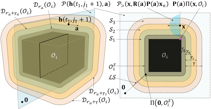
Figure 5: The partition of the set $\mathcal{N}_{\gamma}(\mathcal{D}_{r_{a}}(\mathcal{O}_{i}))\cap\mathcal{P}(\mathbf{h}(t_{1},j_{1}+1),\mathbf{a}(t_{1},j_{1}+1))$.

We show that when the control input corresponds to the obstacle-avoidance mode and the state $\mathbf{x}$ belongs either in the set $\mathcal{S}_{1}$ or in the set $\mathcal{S}_{3}$, the control eventually steers the state $\mathbf{x}$ to the set $\mathcal{S}_{2}.$ Then, we show that for all $\mathbf{x}\in\mathcal{S}_{2}$, the control vector $\mathbf{u}(\xi)$ belongs to the open positive half-space $\mathcal{P}_{>}(\mathbf{0},\mathbf{R}(\mathbf{a}(t_{1},j_{1}+1))\mathbf{P}(\mathbf{a}(t_{1},j_{1}+1))\mathbf{x}_{\pi})$. This implies that the state $\mathbf{x}$, which belongs to the set $\mathcal{N}_{\gamma}(\mathcal{D}_{r_{a}}(\mathcal{O}_{i}))\cap\mathcal{P}(\mathbf{h}(t_{1},j_{1}+1),\mathbf{a}(t_{1},j_{1}+1))$ after time $(t_{1},j_{1})$, in the obstacle-avoidance mode around obstacle $\mathcal{O}_{i}$, is always steered to the open positive half-space $\mathcal{P}_{>}(\mathbf{x},\mathbf{R}(\mathbf{a}(t_{1},j_{1}+1))\mathbf{P}(\mathbf{a}(t_{1},j_{1}+1))\mathbf{x}_{\pi})$ and will eventually reach the set $\mathcal{LS}$ at some finite time $(t_{2},j_{1}+1)\succ(t_{1},j_{1}+1).$

First we show that when the control input corresponds to the obstacle-avoidance mode and the state $\mathbf{x}$ is either in the set $\mathcal{S}_{1}$ or in the set $\mathcal{S}_{3}$, the control will eventually steer the state $\mathbf{x}$ to the set $\mathcal{S}_{2}.$ When the control input corresponds to the obstacle-avoidance mode and $\mathbf{x}$ belongs to the set $\mathcal{S}_{1}$, the control vector $\mathbf{u}(\xi)$ in (11a) becomes

$$\mathbf{u}(\xi)=\kappa_{r}{\mathbf{P}(\mathbf{a}(t_{1},j_{1}+1))\mathbf{x}_{\pi}},\kappa_{r}>0.$$ (48)

For all $\mathbf{x}\in\partial\mathcal{D}_{r_{a}+\beta}(\mathcal{O}_{i}),\beta\in[0,\gamma_{a}]$, according to claim 1 in Lemma 4, one has $\mathbf{u}(\xi)\in(\mathbf{T}_{(\mathcal{S}_{1}\cup\mathcal{S}_{2})\setminus\mathcal{D}_{r_{a}+\beta}^{\circ}(\mathcal{O}_{i})}(\mathbf{x}))^{\circ}$. This implies that when the control input corresponds to the obstacle-avoidance mode, it will steer the state $\mathbf{x}$ towards the interior of the set $(\mathcal{S}_{1}\cup\mathcal{S}_{2})\setminus\mathcal{D}_{r_{a}+\beta}^{\circ}(\mathcal{O}_{i})$ and eventually $\mathbf{x}$ will enter in the set $\mathcal{S}_{2}$.

Similarly, when the control input corresponds to the obstacle-avoidance mode and $\mathbf{x}$ belongs to the set $\mathcal{S}_{3}$, the control vector $\mathbf{u}(\xi)$ in (11a) is given by

$$\mathbf{u}(\xi)=-\kappa_{r}{\mathbf{P}(\mathbf{a}(t_{1},j_{1}+1))\mathbf{x}_{\pi}},\kappa_{r}>0.$$ (49)

For all $\mathbf{x}\in\partial\mathcal{D}_{r_{a}+\beta}(\mathcal{O}_{i}),\beta\in[\gamma_{s},\gamma]$, according to claim 1 in Lemma 4, one has $\mathbf{u}(\xi)\in(\mathbf{T}_{(\mathcal{S}_{3}\cup\mathcal{S}_{2})\cap\mathcal{D}_{r_{a}+\beta}(\mathcal{O}_{i})}(\mathbf{x}))^{\circ}$. This implies that when the control input corresponds to the obstacle-avoidance mode, it will steer the state $\mathbf{x}$ towards the interior of the set $(\mathcal{S}_{3}\cup\mathcal{S}_{2})\cap\mathcal{D}_{r_{a}+\beta}(\mathcal{O}_{i})$ and eventually $\mathbf{x}$ will enter in the set $\mathcal{S}_{2}$.

Finally, we show that when the control input corresponds to the obstacle-avoidance mode and the state $\mathbf{x}$ belongs to the set $\mathcal{S}_{2}$, the control vector $\mathbf{u}(\xi)$ belongs to the open positive half-space $\mathcal{P}_{>}(\mathbf{0},\mathbf{R}(\mathbf{a}(t_{1},j_{1}+1))\mathbf{P}(\mathbf{a}(t_{1},j_{1}+1))\mathbf{x}_{\pi})$. When the control law operates in the obstacle-avoidance mode and the state $\mathbf{x}\in\mathcal{S}_{2}$, according to (11), one has $\mathbf{u}(\xi)=\kappa_{r}\mathbf{v}(\mathbf{x},\mathbf{a}(t_{1},j_{1}+1)),\kappa_{r}>0.$ According to (12), it can be confirmed that $\mathbf{v}(\mathbf{x},\mathbf{a}(t_{1},j_{1}+1))^{\intercal}\mathbf{R}(\mathbf{a}(t_{1},j_{1}+1))\mathbf{P}(\mathbf{a}(t_{1},j_{1}+1))\mathbf{x}_{\pi}>0$, when the state $\mathbf{x}$ belongs to the set $\mathcal{S}_{2},$ and the proof is complete.

References

- [1] O. Khatib, “Real-time obstacle avoidance for manipulators and mobile robots,” in Autonomous robot vehicles. Springer, 1986, pp. 396–404.
- [2] D. E. Koditschek and E. Rimon, “Robot navigation functions on manifolds with boundary,” Advances in applied mathematics, vol. 11, no. 4, pp. 412–442, 1990.
- [3] D. Koditschek and E. Rimon, “Exact robot navigation using artificial potential functions,” IEEE Trans. Robot. Automat, vol. 8, pp. 501–518, 1992.
- [4] C. K. Verginis and D. V. Dimarogonas, “Adaptive robot navigation with collision avoidance subject to 2nd-order uncertain dynamics,” Automatica, vol. 123, p. 109303, 2021.
- [5] C. Li and H. G. Tanner, “Navigation functions with time-varying destination manifolds in star worlds,” IEEE Transactions on Robotics, vol. 35, no. 1, pp. 35–48, 2018.
- [6] S. Paternain, D. E. Koditschek, and A. Ribeiro, “Navigation functions for convex potentials in a space with convex obstacles,” IEEE Transactions on Automatic Control, vol. 63, no. 9, pp. 2944–2959, 2017.
- [7] S. Berkane, “Navigation in unknown environments using safety velocity cones,” in American Control Conference, 2021, pp. 2336–2341.
- [8] F. Blanchini, S. Miani et al., Set-theoretic methods in control. Springer, 2008, vol. 78.
- [9] M. F. Reis, A. P. Aguiar, and P. Tabuada, “Control barrier function-based quadratic programs introduce undesirable asymptotically stable equilibria,” IEEE Control Systems Letters, vol. 5, no. 2, pp. 731–736, 2020.
- [10] O. Arslan and D. E. Koditschek, “Sensor-based reactive navigation in unknown convex sphere worlds,” The International Journal of Robotics Research, vol. 38, no. 2-3, pp. 196–223, 2019.
- [11] V. Vasilopoulos and D. E. Koditschek, “Reactive navigation in partially known non-convex environments,” in Algorithmic Foundations of Robotics XIII. Springer International Publishing, 2020, pp. 406–421.
- [12] S. Berkane, A. Bisoffi, and D. V. Dimarogonas, “Obstacle avoidance via hybrid feedback,” IEEE Transactions on Automatic Control, vol. 67, no. 1, pp. 512–519, 2021.
- [13] A. S. Matveev, H. Teimoori, and A. V. Savkin, “A method for guidance and control of an autonomous vehicle in problems of border patrolling and obstacle avoidance,” Automatica, vol. 47, no. 3, pp. 515–524, 2011.
- [14] S. G. Loizou, H. G. Tanner, V. Kumar, and K. J. Kyriakopoulos, “Closed loop motion planning and control for mobile robots in uncertain environments,” in IEEE Conference on Decision and Control, vol. 3, 2003, pp. 2926–2931.
- [15] M. Sawant, S. Berkane, I. Polushin, and A. Tayebi, “Hybrid feedback for autonomous navigation in planar environments with convex obstacles,” IEEE Transactions on Automatic Control, vol. 68, no. 12, pp. 7342–7357, 2023.
- [16] R. Goebel, R. G. Sanfelice, and A. R. Teel, Hybrid dynamical systems. Princeton University Press, 2012.
- [17] J. Rataj and M. Zähle, Curvature measures of singular sets. Springer, 2019.
- [18] R. G. Sanfelice, Hybrid feedback control. Princeton University Press, 2021.