\ul
Effects of model misspecification on small area estimators
Abstract
Nested error regression models are commonly used to incorporate observational unit specific auxiliary variables to improve small area estimates. When the mean structure of this model is misspecified, there is generally an increase in the mean square prediction error (MSPE) of Empirical Best Linear Unbiased Predictors (EBLUP). Observed Best Prediction (OBP) method has been proposed with the intent to improve on the MSPE over EBLUP. We conduct a Monte Carlo simulation experiment to understand the effect of mispsecification of mean structures on different small area estimators. Our simulation results lead to an unexpected result that OBP may perform very poorly when observational unit level auxiliary variables are used and that OBP can be improved significantly when population means of those auxiliary variables (area level auxiliary variables) are used in the nested error regression model or when a corresponding area level model is used. Our simulation also indicates that the MSPE of OBP in an increasing function of the difference between the sample and population means of the auxiliary variables.
Keywords: Model misspecification; Small area estimation; OBP; EBLUP
1 Introduction
Direct survey-weighted estimates (e.g., Cochran, 1977) are routinely used for producing a wide range of socio-economic, environment, health, and other official statistics for national and large sub-national areas. When the targets are smaller geographical areas, the issue of having a limited or no sample can render direct estimates unreliable. Therefore, small area estimation (SAE) has garnered increasing attention in recent decades, as it is used to leverage strength from related data sources such as census, administrative and geo-spatial data through statistical modeling. For a comprehensive review of various SAE methods and models, we refer to Rao and Molina (2015).
In this section, for simplicity of exposition, we assume that a simple random sample (SRS) is selected for each small area. Suppose that the values of auxiliary variables are known for every unit in the finite population. Battese et al. (1988) introduced the following nested error regression model that links the response variable to the auxiliary variables for each unit of the finite population:
| (1.1) |
where is the number of areas; is known population size of area ; ’s are area-specific random effect; ’s are sampling errors. We assume that and are independent with and . In general, regression coefficients and the variance components and are unknown.
The following special case of the nested error regression model, often referred to as unit-context model, has received considerable attention in recent years; see, e.g., Newhouse et al. (2022). The model can be written as:
| (1.2) |
where is a vector of known area-specific auxiliary variables. We make the same assumptions on the random effects and sampling errors These models offer an alternative approach when unit level auxiliary variables (e.g., say from census records) are either unavailable or too outdated to be used as unit-specific auxiliary variables but area specific auxiliary variables are available (e.g., from geo-spatial data).
Area-level model, introduced by Fay III and Herriot (1979), can be another possibility to handle lack of good unit-specific auxiliary variables. It models area level direct estimates of the parameter of interest to area-level auxiliary variables, and assumes the form:
| (1.3) |
where is direct estimate from survey; is a vector of known area-level auxiliary variables; ’s are area-specific random effect; ’s are sampling errors. It is assumed that ’s and ’s are independent with , . The variance of sampling errors, , is commonly assumed to be known, but in practice they are estimated using a smoothing technique such as the one given in Otto and Bell (1995).
The Best Predictor (BP) of a mixed effect in a linear mixed model is simply the conditional mean of the mixed effect given the data. Conceptually this BP can be obtained under a full specification of the distributions of the random effects and errors. When conditional mean of the random effects given the data is assumed to be a linear function of the sample observations, an explicit formula for BP can be obtained. The Best Linear Unbiased Predictor (BLUP) is obtained from the Best Predictor (BP) under the assumed linear mixed model when the unknown regression coefficients in the BP is replaced by the weighted least square estimators. Estimated BLUP (EBLUP) is obtained when the unknown variance components of the model are replaced by standard estimators (e.g., REML). The BLUP and EBLUP can be viewed as an estimated BP (EBP) of the mixed effects.
Jiang et al. (2011) proposed Observed Best Predictors (OBP) for small area means under a linear mixed model in an attempt to reduce the effects of misspecification of the mean structure in the assumed model. We note that their OBP can be motivated as EBP when best predictive estimators (BPE) of model parameters, which minimize the observed mean squared prediction error (MPSE), are used in place of standard model parameter estimators. In the context of area level models, Jiang et al. (2011) used both theoretical and empirical studies to demonstrate that OBP outperforms EBLUP in terms of MPSE when the underlying linear mixed model is misspecified. Subsequently, Jiang et al. (2015) considered OBP for nested error regression model, where both the mean function and variance components are misspecified. Their simulations indicated that OBP may perform significantly better than EBLUP in terms of both overall MSPE and area-specific MSPE.
In this paper, we investigate the effects of misspecified mean function and variance components on the predictive performances of existing small area estimators. The rest of the paper is organized as follows. In Section 2, we present numerical studies and the evaluation results in terms of both overall MSPE and area-specific MSPE. In Section 3, we summarize and conclude our paper by giving some practical guidelines on implementing OBP to handle model misspecification issues.
2 Simulations
The derivations of OBP procedure for both area-level and unit-level models can be found in the supplementary materials of Jiang et al. (2011). Also, since unit-context model is a special type of unit-level models, we can directly derive OBP by replacing by .
The simulation settings are similar to Jiang et al. (2015). For simplicity, we consider a case of a single auxiliary variable that is assumed to be linearly associated with the response variable through the following model:
| (2.1) |
where ’s are known values of an auxiliary variable for the th unit of the th area; is an unknown regression coefficient; , are the same as in (1.1). We assume that ’s are not all the same in an area. In the present context, (1.2) becomes:
| (2.2) |
And, the corresponding area-level model is given by:
| (2.3) |
For the simulations set up, we draw simple random sampling without replacement (SRSWOR) samples from the population of each small areas and consider the following estimators of the small area means throughout the rest of this section:
-
(A)
Direct estimator (sample mean),
-
(B)
OBP under the assumed unit-context model (OBP-UC),
-
(C)
OBP under the basic Fay-Herriot (area-level) model with known sampling variance calculated from the simulated population of the small areas (OBP-FH),
-
(D)
OBP under the assumed unit-level model (OBP-UNIT),
-
(E)
EBLUP under the assumed unit-level model (EBLUP).
To introduce model misspecifications, we first generate for the finite population from the following superpopulation heteroscedastic nested-error regression model:
| (2.4) |
The population and sample sizes are the same for all areas and are fixed at and , respectively. We consider two different values of : , and three values of the number of small areas: or with generated from the normal distribution , and generated from the normal distribution , where is independently generated from the gamma distribution . In each case, for the finite population is generated from a log-normal superpopulation distribution with a mean of 1 and a standard deviation of 0.5.
Each scenario is independently simulated times. The performance of the estimators (A)-(E), under the above simulation setups, are assessed in terms of both overall and area-specific MSPEs. The area-specific MSPE is defined as , where is the true small area mean, and is the predicted value for th area, either by OBP or EBLUP. In Monte Carlo simulations, MSPE for area and overall MSPE are approximated by:
| (2.5) |
| (2.6) |
respectively, where and are the true mean and estimated mean for area in the simulation run, respectively.
| DIRECT | OBP-UC | OBP-FH | OBP-UNIT | EBLUP | |
|---|---|---|---|---|---|
| (40, 5) | 1.475 | 0.689 | 0.630 | 1.775 | 1.474 |
| (100, 5) | 1.488 | 0.638 | 0.588 | 1.409 | 1.495 |
| (400, 5) | 1.493 | 0.614 | 0.567 | 1.352 | 1.508 |
| (40, 10) | 1.475 | 0.696 | 0.636 | 3.919 | 1.522 |
| (100, 10) | 1.488 | 0.646 | 0.595 | 2.364 | 1.513 |
| (400, 10) | 1.493 | 0.621 | 0.574 | 1.711 | 1.510 |
Table 2.1 reports the simulated overall MSPE for the various simulation conditions and estimators under the true underlying model (2.4). First of all, direct estimator is not affected by model misspecification because it is not model based. EBLUP behavior is similar to direct because it automatically assigns more weight to the sample mean when the model is weak. Surprisingly, the performance of OBP-UNIT is worse than OBP-UC in all cases considered. Moreover, note that the simulated overall MSPE is even larger than those of direct estimators and EBLUPs with . Also, OBP-UC performs much better than OBP-UNIT. The performance of OBP-UC is similar to OBP-FH in which is calculated from the entire population. The findings suggest that in instances of significant model misspecification, OBP-UNIT may not be recommended.
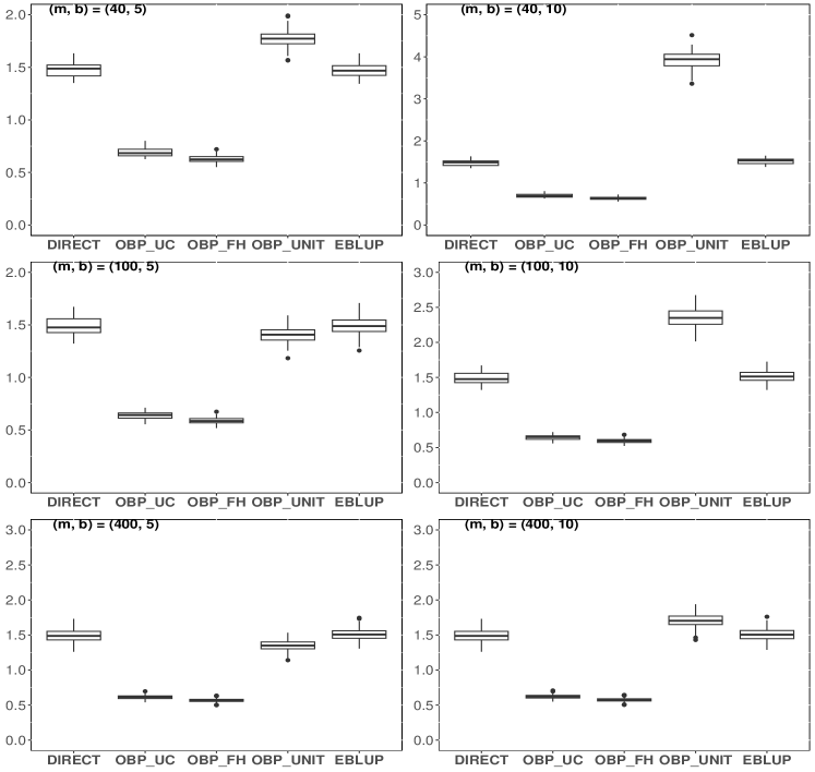
As for the area-specific MSPEs, we utilize boxplots to display the distributions of the area-specific MSPEs associated with all the estimators. See Figure 2.1. The boxplot of OBP-UNIT shows much larger median MSPE and variability than those of OBP-UC and OBP-FH and in some cases worse than direct and EBLUP. OBP-UC shows slightly larger variability than OBP-FH. It might be because that in contrast to area-level models, unit-context models incorporate the uncertainty resulting from the estimation of model parameters, such as sampling variances.
As discussed in Jiang et al. (2015), the simulation conditions above might be a little extreme in which the assumed models are completely different from the true underlying model. This motivates us to consider some moderate cases where assumed model is partially correct compared to the true model. Keeping the same assumed models (2.1) - (2.3) we generate the finite population for from the underlying superpopulation model:
| (2.7) |
where , . Note that the slope in (2.7) is not zero and it matches the linear relationship part of the assumed model (2.1). But still, we have slight misspecifications in the sense that the true model here also has a nonzero intercept. In addition, is generated from the same normal distribution as described previously, and so we have the issue of heteroscedasticity as well. Three different values of are considered: or , and is generated from normal distribution .
The results based on simulations are displayed in Table 2.2. As expected, in this case EBLUP now performs much better than the direct estimator as the assumed model is closer to the true model. OBP-UNIT performs better than direct estimator for larger , but performs worse than EBLUP in all situations. The performance of OBP-UC and OBP-FH is similar, especially both of them perform much better than OBP-UNIT and performs better than EBLUP for large ,
| DIRECT | OBP-UC | OBP-FH | OBP-UNIT | EBLUP | |
|---|---|---|---|---|---|
| 40 | 18.243 | 1.798 | 1.837 | 18.230 | 1.532 |
| 100 | 18.339 | 1.341 | 1.385 | 7.958 | 1.514 |
| 400 | 18.422 | 1.085 | 1.099 | 3.122 | 1.509 |
2.1 Remark
To further investigate the failure of OBP with misspecified unit-specific auxiliary variables, we undertake a numerical study to evaluate the association between (absolute difference between the th area sample mean and population mean) and th area , approximated by Monte Carlo. First, we generate the finite population for using the following NER superpopulation model:
| (2.8) |
The generative processes for the finite population for , , and remain consistent with the aforementioned model. Subsequently, we draw SRS samples of size from the population of each small areas.
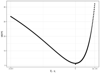
In a simulation setting, when the number of units within a specific area is relatively small, it is often impossible to have sample mean equal or even close to population mean . Therefore, in this subsection, we manually change the realizations of sample means by letting , where the bias term assumes negative, positive, and zero values. Figure 2.2 demonstrates that simulated for the OBP with unit level auxiliary variables increases with the difference between and for area (for other areas, figures are similar). Notably, when , i.e., for the unit-context model, simulated is observed to be smaller than corresponding values for any other instances of .
3 Conclusion
In this paper, we investigate the effects of misspecified mean structure and sampling variance in the well-known nested error regression model on EBLUP and OBP that uses (i) unit-level auxiliary variables only and (ii) area-level auxiliary variables only (i.e., unit context model). Through simulated scenarios, we illustrate that, in the presence of substantial model misspecifications, OBP procedure for unit context model shows better performance than that of the corresponding unit-level model using unit-specific auxiliary variables. Also, with known sampling variances, the performance of OBP under area-level model and unit-context model is similar, and both are better than the OBP using unit-specific auxiliary variables. These findings suggest that implementing the OBP procedure within unit-context models could be a viable alternative when faced with challenges such as the absence of census information and/or potential model misspecification issues. While we do not have a clear understanding why OBP for nested error model with solely unit level auxiliary variables performs poorly in our simulation study, it appears that the difference between the sample and population means of the auxiliary variables could be a potential factor. We encourage further theoretical and empirical research to understand this unexpected behavior of OBP for nested error model with solely unit level auxiliary variables.
References
- Battese et al. (1988) Battese, G. E., R. M. Harter, and W. A. Fuller (1988). An error-components model for prediction of county crop areas using survey and satellite data. Journal of the American Statistical Association 83(401), 28–36.
- Cochran (1977) Cochran, W. G. (1977). Sampling techniques. john wiley & sons.
- Fay III and Herriot (1979) Fay III, R. E. and R. A. Herriot (1979). Estimates of income for small places: an application of james-stein procedures to census data. Journal of the American Statistical Association 74(366a), 269–277.
- Jiang et al. (2011) Jiang, J., T. Nguyen, and J. S. Rao (2011). Best predictive small area estimation. Journal of the American Statistical Association 106(494), 732–745.
- Jiang et al. (2015) Jiang, J., T. Nguyen, and J. S. Rao (2015). Observed best prediction via nested-error regression with potentially misspecified mean and variance. Survey Methodology 41(1), 37–56.
- Newhouse et al. (2022) Newhouse, D. L., J. D. Merfeld, A. Ramakrishnan, T. Swartz, and P. Lahiri (2022). Small area estimation of monetary poverty in mexico using satellite imagery and machine learning. Available at SSRN 4235976.
- Otto and Bell (1995) Otto, M. C. and W. R. Bell (1995). Sampling error modelling of poverty and income statistics for states. In American Statistical Association, Proceedings of the Section on Government Statistics, pp. 160–165.
- Rao and Molina (2015) Rao, J. N. and I. Molina (2015). Small area estimation. John Wiley & Sons.