Understanding Diffusion Models by Feynman’s Path Integral

Abstract

Score-based diffusion models have proven effective in image generation and have gained widespread usage; however, the underlying factors contributing to the performance disparity between stochastic and deterministic (i.e., the probability flow ODEs) sampling schemes remain unclear. We introduce a novel formulation of diffusion models using Feynman’s path integral, which is a formulation originally developed for quantum physics. We find this formulation providing comprehensive descriptions of score-based generative models, and demonstrate the derivation of backward stochastic differential equations and loss functions. The formulation accommodates an interpolating parameter connecting stochastic and deterministic sampling schemes, and we identify this parameter as a counterpart of Planck’s constant in quantum physics. This analogy enables us to apply the Wentzel–Kramers–Brillouin (WKB) expansion, a well-established technique in quantum physics, for evaluating the negative log-likelihood to assess the performance disparity between stochastic and deterministic sampling schemes.

1 Introduction

Diffusion models have demonstrated impressive performance on image generation tasks (Dhariwal & Nichol, 2021) and they have earned widespread adoption across various applications (Yang et al., 2023). While the predominant contemporary application of diffusion models lies in conditional sampling driven by natural language (Rombach et al., 2022), the mathematical framework underlying their training, i.e., the score-based scheme (Hyvärinen et al., 2009; Vincent, 2011; Song & Ermon, 2019) or the denoising scheme (Sohl-Dickstein et al., 2015; Ho et al., 2020), is not inherently dependent on prior conditions. The work (Kingma et al., 2021) showed the equivalence of these two schemes from a variational perspective. The work (Song et al., 2021b) developed a unified description based on stochastic differential equations (SDEs). In both cases, the sampling process is given by a Markovian stochastic process.

Another type of probabilistic models employs deterministic sampling schemes using ordinary differential equations (ODEs) such as the probability flow ODE (Song et al., 2021b), which can be understood as a continuous normalizing flow (CNF) (Chen et al., 2018; Lipman et al., 2023). A notable advantage of deterministic sampling schemes is that there is a bijective map between the latent space and the data space. This bijection not only facilitates intricate tasks like manipulation of latent representations for image editing (Su et al., 2023) but also enables the direct computation of negative log-likelihoods (NLLs). Within stochastic sampling processes in contrast to deterministic ones, a direct evaluation method of the NLL remains elusive, though a theoretical bound exists for the NLL (Kong et al., 2023).

In general, stochastic sampling schemes require more number of function evaluations (NFE) than deterministic schemes, and is inferior in terms of sample generation speed. However, the beneficial impact of stochastic generation on certain metrics, such as the Fréchet Inception Distance (FID) (Heusel et al., 2017) is a well-known property in practice. For example, (Karras et al., 2022) reports improvements in these metrics with the incorporation of stochastic processes both in Variance-Exploding (VE) and Variance-Preserving pretrained models in (Song et al., 2021b). Intuitively, one can conceptualize noise within stochastic generation as perturbation to propel particles out of local minima, potentially enhancing the diversity and quality of the generated samples. However, beyond this intuitive level, thoroughly quantitative analysis or rigorous theoretical framework to explain this phenomenon is missing.

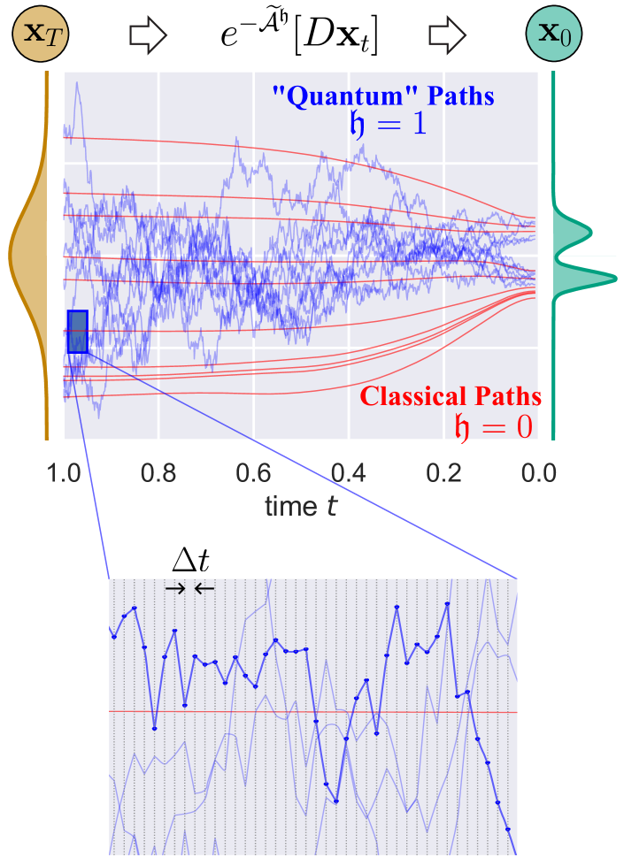
Figure 1: Schematic of the path integral formulation of diffusion models.

We tackle these two issues by making use of the path integral formalism, a framework originally developed in quantum physics by Feynman (Feynman, 1948; Feynman & Hibbs, 1965). In classical physics, a particle’s motion draws a trajectory, i.e., a deterministic path in space and time. To accommodate quantum effects, the path integral formalism generalizes the trajectory including quantum fluctuations by comprising all possible paths, $\{\mathbf{x}_{t}\}_{t\in[0,T]}$, of a particle between two points, $\mathbf{x}_{0}$ at time $t=0$ and $\mathbf{x}_{T}$ at $t=T$; see a magnified panel in Fig. 1 for a counterpart in diffusion models. The quantum expectation value of observable $\mathcal{O}(\mathbf{x}_{t})$ is computed as a weighted sum: $\sum_{\text{paths}}\mathcal{O}(\mathbf{x}_{t})e^{i\mathcal{A}[\mathbf{x}_{t}]/\hbar}$, where $\hbar$ is Planck’s constant. In addition to quantum fluctuations, the path integral can be extended to incorporate stochastic fluctuations as well (Onsager & Machlup, 1953). We demonstrate that diffusion models can be formulated in terms of path integrals, which not only deepens our understanding about diffusion model formulations but also allows for the application of various techniques advanced in quantum physics. Importantly, this framework provides an innovative method for calculating the NLL in stochastic generation processes of diffusion models.

Our contributions are as follows.

• We reformulate diffusion models using path integral techniques. We exemplify applications including a re-derivation of the time-reversed SDE (Anderson, 1982) and an estimate of loss functions (Song et al., 2021a) based on Girsanov’s theorem (Oksendal, 2013).

• Following (Zhang & Chen, 2023), we introduce an interpolating parameter $\mathfrak{h}$ connecting the stochastic generation ($\mathfrak{h}=1$) and the probability flow ODE ($\mathfrak{h}=0$). In the path integral language, the limit $\mathfrak{h}\to 0$ corresponds to the classical limit under which quantum fluctuations are dropped off. The path integral formulation of diffusion models reveals the role of $\mathfrak{h}$ as Planck’s constant $\hbar$ in quantum physics.

• We apply the Wentzel–Kramers–Brillouin (WKB) expansion (Messiah, 1970), that is formulated in terms of Planck’s constant $\hbar$ in quantum physics, with respect to $\mathfrak{h}$ to the likelihood calculation. Based on the first order NLL expression, we quantify the merit of noise in the sampling process by computing the NLL as well as the 2-Wasserstein distance.

Building upon the analogy with quantum physics, these contributions unveil a far more profound connection to physics beyond a classic viewpoint of the Brownian motion.

2 Related works

Diffusion models

Key contributions in this field of diffusion models include (Sohl-Dickstein et al., 2015) and (Song et al., 2021b) which have laid the foundational principles for these models. Our reformulation of diffusion models by path integrals captures the basic mathematical characteristics of score-based diffusion models. The idea of implementing stochastic variables to represent quantum fluctuations is traced back to (Nelson, 1966), and mathematical foundation has been established as stochastic quantization (Damgaard & Hüffel, 1987). Recent works (Wang et al., 2023; Premkumar, 2023) suggested similarity between diffusion models and quantum physics. However, the path integral derivation of the basic aspects of diffusion models has not been discussed. There is no preceding work to explore the WKB expansion applied in diffusion models.

Likelihood calculation in diffusion models

In deterministic sampling schemes based on ODEs, one can directly calculate log-likelihood based on the change-of-variables formula (Chen et al., 2018; Song et al., 2021b; Lipman et al., 2023). Once we turn on noise in the sampling process, only a formal expression is available from the celebrated Feynman-Kac formula (Huang et al., 2021b). To our best knowledge, there is no stochastic case where the values of log-likelihood have ever been calculated. Our approach of the perturbative expansion with respect to $\mathfrak{h}$ can access the log-likelihood explicitly even in the presence of noise. Note that an exact formula for the log-likelihood has been derived based on the information theory connecting to the Minimum Mean Square Error (MMSE) regression (Kong et al., 2023). However, this method still necessitates the computation of expectation values and cannot be implemented using a single trajectory.

Stochastic and deterministic sampling procedures

The role of stochasticity in the sampling process has been investigated in (Karras et al., 2022) through empirical studies. The gap between the score-matching objective depending on the sampling schemes has been pointed out in (Huang et al., 2021a). To bridge the gap between the model distribution generated by the probability flow and the actual data distribution, (Lu et al., 2022) introduced a higher-order score-matching objective. Besides these efforts, (Lai et al., 2023) derived an equation to be satisfied by a score function and introduced a regulator in the loss function to enforce this relation. The present approach is complementary to these works; we employ the perturbative $\mathfrak{h}$-expansion and directly evaluate the noise-strength dependence of the NLL for pretrained models.

3 Reformulation of diffusion models by path integral formalism

In this section, we describe the reformulation of score-based diffusion models in terms of path integrals.

3.1 Forward and reverse processes

For a given datapoint $\mathbf{x}_{0}$ sampled from an underlying data distribution $p_{0}$, the first step of a score-based diffusion model is to gradually modify the data by adding noise via a forward SDE,

$${\rm d}\mathbf{x}_{t}=\bm{f}(\mathbf{x}_{t},t){\rm d}t+g(t){\rm d}\mathbf{w}_{t}.$$ (1)

One can view this diffusion process as a collection of stochastic trajectories, and consider the “path-probability” $P(\{\mathbf{x}_{t}\}_{t\in[0,T]})$ associated with Eq. (1). Intuitively, it corresponds to the joint probability for the “path” $\{\mathbf{x}_{t}\}_{t\in[0,T]}$ (see also Fig. 1 for schematic illustration of paths). In the path integral formulation of quantum mechanics, the expectation value of observables is expressed as a summation over all possible paths weighted by an exponential factor with a quantity called an action. We observe that the process (1) of diffusion models can be represented as a path integral:

Proposition 3.1.

The path-probability $P(\{\mathbf{x}_{t}\}_{t\in[0,T]})$ can be represented in the following path integral form:

$$P(\{\mathbf{x}_{t}\}_{t\in[0,T]}) =p_{0}(\mathbf{x}_{0})e^{-\mathcal{A}}[D\mathbf{x}_{t}],$$ (2)

with $\mathcal{A}\coloneqq\int_{0}^{T}L(\dot{\mathbf{x}}_{t},\mathbf{x}_{t}){\rm d}t+J$, where $L(\dot{\mathbf{x}}_{t},\mathbf{x}_{t})$ is called Onsager–Machlup function (Onsager & Machlup, 1953) defined by

$$L(\dot{\mathbf{x}}_{t},\mathbf{x}_{t})\coloneqq\frac{\|\dot{\mathbf{x}}_{t}-\bm{f}(\mathbf{x}_{t},t)\|^{2}}{2g(t)^{2}},$$

and $J$ is the Jacobian associated with the chosen discretization scheme in stochastic process.

Here, the overdot indicates the time derivative. In the physics literature, $L(\dot{\mathbf{x}}_{t},\mathbf{x}_{t})$ is called the Lagrangian and $\mathcal{A}$ is the action. For a detailed derivation of Eq. 2 and the explicit expression for $J$, see Sec. A.2.

Using the path probability (2), the expectation value of any observable $\mathcal{O}(\mathbf{x}_{t})$ depending on $\mathbf{x}_{t}$ obeying Eq. 1 is represented as $\mathbb{E}[\mathcal{\mathcal{missing}}O(\mathbf{x}_{t})]=\int O(\mathbf{x}_{t})P(\{\mathbf{x}_{t}\}_{t\in[0,T]})$. This expression is commonly referred to as a path integral as it involves the summation over infinitely many paths.

Here, we present an intuitive explanation of the expression (2). Let us start from a discretized version of the SDE (1) by Euler-Maruyama scheme:

$$\mathbf{x}_{t+\Delta t}=\mathbf{x}_{t}+\bm{f}(\mathbf{x}_{t},t)\Delta t+g(t)\sqrt{\Delta t}\mathbf{v}_{t},\quad\mathbf{v}_{t}\sim\mathcal{N}(\mathbf{0},I),$$

$$\Leftrightarrow p(\mathbf{x}_{t+\Delta t}|\mathbf{x}_{t})=\mathcal{N}(\mathbf{x}_{t+\Delta t}|\mathbf{x}_{t}+\bm{f}(\mathbf{x}_{t},t)\Delta t,g(t)^{2}\Delta tI),$$

where $\Delta t$ is time interval and $I$ is the identity matrix. Now the time evolution of the SDE is described by a conditional Gaussian distribution. In the following, we take $\mathbf{x}_{t+\Delta t}-\mathbf{x}_{t}\approx\dot{\mathbf{x}}_{t}\Delta t$, and deform the conditional Gaussian as

$$p(\mathbf{x}_{t+\Delta t}|\mathbf{x}_{t}) \propto e^{-\frac{\|\dot{\mathbf{x}}_{t}-\bm{f}(\mathbf{x}_{t},t)\|^{2}}{2g(t)^{2}}\Delta t}=e^{-L(\dot{\mathbf{x}}_{t},\mathbf{x}_{t})\Delta t}.$$

Now let us consider the probability for realizing an explicit “path” $\{\mathbf{x}_{t}\}:=[\mathbf{x}_{0},\mathbf{x}_{\Delta t},\mathbf{x}_{2\Delta t},\cdots,\mathbf{x}_{T}]$, and regarding the summation as the Riemannian sum, we get the following path integral expression for the path probability:

$$\begin{split}&p_{0}(\mathbf{x}_{0})p(\mathbf{x}_{\Delta t}|\mathbf{x}_{0})\cdots p(\mathbf{x}_{T}|\mathbf{x}_{T-\Delta t})\prod_{t}{\rm d}\mathbf{x}_{t}\\ &\eqqcolon p_{0}(\mathbf{x}_{0})e^{-\sum_{n=0}^{T/\Delta t-1}L(\dot{\mathbf{x}}_{n\Delta t},\mathbf{x}_{n\Delta t})\Delta t}[D\mathbf{x}_{t}]_{\Delta t},\end{split}$$ (3)

where $[D\mathbf{x}_{t}]_{\Delta t}$ contains a normalization constant depending on the discretization step $\Delta t$. We take the $\Delta t\to 0$ limit at the end of the calculation and omit $\Delta t$ in the subscript in later discussions. In the expression (3), we need to include an additional contribution denoted by $J$ in Proposition 3.1, depending on the choice of the discretization scheme (see Sec. A.2 for details).

The sampling process of score-based diffusion models is realized by the time-reversed version of the forward SDE (1). The path integral reformulation is beneficial in furnishing an alternative derivation of the reverse-time SDE:

Proposition 3.2.

Let $P(\{\mathbf{x}_{t}\}_{t\in[0,T]})$ be the path-probability, and $p_{t}(\mathbf{x})$ be the distribution at time $t$ determined by the Fokker-Planck equation corresponding to Eq. 1. The path-probability is written using the reverse-time action $\widetilde{\mathcal{A}}$ as

$$P(\{\mathbf{x}_{t}\}_{t\in[0,T]}) =e^{-\widetilde{\mathcal{A}}}\,p_{T}(\mathbf{x}_{T})[D\mathbf{x}_{t}],$$

with $\widetilde{\mathcal{A}}\coloneqq\int_{0}^{T}\widetilde{L}(\dot{\mathbf{x}}_{t},\mathbf{x}_{t}){\rm d}t+\widetilde{J}$, where

$$\widetilde{L}(\dot{\mathbf{x}}_{t},\mathbf{x}_{t}) \coloneqq\frac{\|\dot{\mathbf{x}}_{t}-\bm{f}(\mathbf{x}_{t},t)+g(t)^{2}\nabla\log p_{t}(\mathbf{x}_{t})\|^{2}}{2g(t)^{2}},$$

and $\widetilde{J}$ is the Jacobian for reverse process depending on the discretization scheme.

We provide the proof in Sec. A.3. We emphasize that the path integral derivation does not rely on the reverse-time SDE (Anderson, 1982). In fact, $\widetilde{L}$ involves the score-function $\nabla\log p_{t}(\mathbf{x}_{t})$, so that Proposition 3.2 gives us another derivation of the reverse-time SDE,

$${\rm d}\mathbf{x}_{t}=[\bm{f}(\mathbf{x}_{t},t)-g(t)^{2}\nabla\log p_{t}(\mathbf{x}_{t})]{\rm d}t+g(t){\rm d}\bar{\mathbf{w}}_{t},$$ (4)

by inverting the discussion from Eq. 1 to Proposition 3.1.

3.2 Models and objectives

In score-based models (Song & Ermon, 2019; Song et al., 2021a, b), the score function $\nabla\log p_{t}(\mathbf{x}_{t})$ is approximated by a neural network $\bm{s}_{\theta}(\mathbf{x}_{t},t)$, and samplings are performed based on

$${\rm d}\mathbf{x}_{t}=[\bm{f}(\mathbf{x}_{t},t)-g(t)^{2}\bm{s}_{\theta}(\mathbf{x}_{t},t)]{\rm d}t+g(t){\rm d}\bar{\mathbf{w}}_{t},$$ (5)

that is a surrogate for the reverse-time (4). By repeating the same argument as Proposition 3.2, we can conclude that the path-probability $Q_{\theta}(\{\mathbf{x}_{t}\})$ corresponding to Eq. 5 takes the following path integral representation:

$$Q_{\theta}(\{\mathbf{x}_{t}\}) =e^{-\widetilde{\mathcal{A}}_{\theta}}\pi(\mathbf{x}_{T})[D\mathbf{x}_{t}],$$ (6)

where $\pi(\cdot)$ is a prior distribution, typically chosen to be the standard normal distribution. Here, $\widetilde{\mathcal{A}}_{\theta}\coloneqq\int_{0}^{T}\widetilde{L}_{\theta}(\dot{\mathbf{x}}_{t},\mathbf{x}_{t}){\rm d}t+\widetilde{J}_{\theta}$ with $\widetilde{L}_{\theta}$ the Onsager–Machlup function for the SDE (5) defined by

$$\widetilde{L}_{\theta}(\dot{\mathbf{x}}_{t},\mathbf{x}_{t}) \coloneqq\frac{\|\dot{\mathbf{x}}_{t}-\bm{f}(\mathbf{x}_{t},t)+g(t)^{2}\bm{s}_{\theta}(\mathbf{x}_{t},t)\|^{2}}{2g(t)^{2}},$$ (7)

and $\widetilde{J}_{\theta}$ is the Jacobian contribution. Figure 1 depicts a schematic picture of these reverse-time processes.

Now, we can follow the training scheme based on bound of the log-likelihood or equivalently, KL divergence via data-processing inequality (Song et al., 2021a):

$$D_{\rm KL}(p_{0}\|{q_{\theta}}_{0})\leq D_{\rm KL}(P\|Q_{\theta}).$$ (8)

The r.h.s. of Eq. 8 can be calculated by using Girsanov’s theorem (Oksendal, 2013). An equivalent computation can also be performed in the path integral formulation:

Proposition 3.3.

The KL divergence of path-probabilities can be represented by the path integral form,

$$D_{\rm KL}(P\|Q_{\theta}) =\int e^{-\widetilde{\mathcal{A}}}p_{T}(\mathbf{x}_{T})\log\frac{e^{-\widetilde{\mathcal{A}}}\,p_{T}(\mathbf{x}_{T})}{e^{-\widetilde{\mathcal{A}}_{\theta}}\pi(\mathbf{x}_{T})}[D\mathbf{x}_{t}],$$

and it can be computed as

$$D_{\rm KL}(P\|Q_{\theta})=D_{\rm KL}(p_{T}\|\pi)$$

$$\quad\quad+\int_{0}^{T}\frac{g(t)^{2}}{2}\mathbb{E}_{p_{t}}\|\nabla\log p_{t}(\mathbf{x}_{t})-\bm{s}_{\theta}(\mathbf{x}_{t},t)\|^{2}{\rm d}t.$$

Indeed, Proposition 3.3 yields the same contribution as the calculation based on Girsanov’s theorem. We give the derivation of Proposition 3.3 in Sec. A.4.

The discussion so far can be straightforwardly extended to the cases with fixed initial conditions. One can basically make the replacement, $p_{t}(\mathbf{x}_{t})\to p_{t}(\mathbf{x}_{t}|\mathbf{x}_{0})$; see Sec. A.5 for details.

4 Log-likelihood by WKB expansion

We have so far discussed reformulation of score-based diffusion models using the path integral formalism. This reformulation allows for the techniques developed in quantum physics for analyzing the properties of diffusion models. As an illustrative example, we present the calculation of log-likelihood in the presence of noise in the sampling process by pretrained models.

4.1 Interpolating SDE and probability flow ODE

Following (Zhang & Chen, 2023), we consider a family of generating processes defined by the following SDE parametrized by $\mathfrak{h}\in\mathbb{R}_{\geq 0}$:

$${\rm d}\mathbf{x}_{t}=\left[\bm{f}(\mathbf{x}_{t},t)-\frac{1+{\mathfrak{h}}}{2}g(t)^{2}\bm{s}_{\theta}(\mathbf{x}_{t},t)\right]{\rm d}t+{\sqrt{\mathfrak{h}}}g(t){\rm d}\bar{\mathbf{w}}_{t}.$$ (9)

If we take $\mathfrak{h}=0$, the noise term vanishes, and the process reduces to the probability flow ODE (Song et al., 2021b). The situation at $\mathfrak{h}=1$ corresponds to the original SDE (5). The path-probability corresponding to this process (9) can be expressed as

$$Q_{\theta}^{\mathfrak{h}}(\{\mathbf{x}_{t}\}_{t\in[0,T]}) =e^{-\widetilde{\mathcal{A}}_{\theta}^{\mathfrak{h}}}\pi(\mathbf{x}_{T})[D\mathbf{x}_{t}],$$ (10)

with $\widetilde{\mathcal{A}}_{\theta}^{\mathfrak{h}}\coloneqq\int_{0}^{T}\widetilde{L}_{\theta}^{\mathfrak{h}}(\dot{\mathbf{x}}_{t},\mathbf{x}_{t}){\rm d}t+\widetilde{J}_{\theta}^{\mathfrak{h}}$, where

$$\widetilde{L}_{\theta}^{\mathfrak{h}}(\dot{\mathbf{x}}_{t},\mathbf{x}_{t})\coloneqq\frac{\|\dot{\mathbf{x}}_{t}-\bm{f}(\mathbf{x}_{t},t)+\frac{1+\mathfrak{h}}{2}g(t)^{2}\bm{s}_{\theta}(\mathbf{x}_{t},t)\|^{2}}{2\mathfrak{h}g(t)^{2}},$$ (11)

and $\widetilde{J}_{\theta}^{\mathfrak{h}}$ is the Jacobian contribution.

The way how $\mathfrak{h}$ enters Eq. 11 is quite suggestive: the action $\widetilde{\mathcal{A}}^{\mathfrak{h}}_{\theta}$ is inversely proportional to $\mathfrak{h}$, similarly to quantum mechanics where the path integral weight takes a form of $e^{-i\mathcal{A}/\hbar}$. This structural similarity provides us with a physical interpretation of the limit, $\mathfrak{h}\to 0$; it realizes the classical limit in the path integral representation. Moreover, this analogy between $\mathfrak{h}$ and $\hbar$ naturally leads us to explore a perturbative expansion in terms of $\mathfrak{h}$, i.e., the WKB expansion, a well-established technique to treat the asymptotic series expansion in mathematical physics.

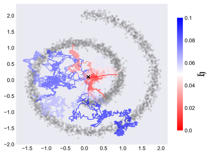
Figure 2: Gray dots: training data. Colored lines: generative trajectories based on Eq. 9 for different noise levels $\mathfrak{h}$ from the identical initial vector $\mathbf{x}_{T}$ shown by $\times$.

In the classical limit of $\mathfrak{h}\to 0$, the dominant contribution comes from the path that minimizes the action, realizing the principle of least action in the physics context. Since the Lagrangian $\widetilde{L}^{\mathfrak{h}}_{\theta}$ of this model is nonnegative, $e^{-\widetilde{\mathcal{A}}^{\mathfrak{h}}_{\theta}}$ goes vanishing in the limit $\mathfrak{h}\to 0$ unless the path satisfies $\widetilde{L}^{\mathfrak{h}=0}_{\theta}=0$ or equivalently $\dot{\mathbf{x}}=\bm{f}_{\theta}^{\text{PF}}(\mathbf{x}_{t},t)$, where $\bm{f}_{\theta}^{\text{PF}}(\mathbf{x}_{t},t)$ is the drift term for the probability flow ODE defined by

$$\bm{f}_{\theta}^{\text{PF}}(\mathbf{x}_{t},t)\coloneqq\bm{f}(\mathbf{x}_{t},t)-\frac{1}{2}g(t)^{2}\bm{s}_{\theta}(\mathbf{x}_{t},t).$$ (12)

Consequently, the path-probability reduces to the product of delta functions as $\mathfrak{h}\to 0$:

$$e^{-\widetilde{\mathcal{A}}_{\theta}^{\mathfrak{h}}}\pi(\mathbf{x}_{T})[D\mathbf{x}_{t}]$$

$$\to\left(\prod_{t=0}^{T}\delta\bigl{(}\dot{\mathbf{x}}_{t}-\bm{f}_{\theta}^{\text{PF}}(\mathbf{x}_{t},t)\bigr{)}\right)e^{-\tilde{J}^{\mathfrak{h}=0}_{\theta}}\pi(\mathbf{x}_{T})[D\mathbf{x}_{t}].$$

This situation is visualized in Fig. 2: we plot trajectories generated by the SDE (9) from fixed $\mathbf{x}_{T}$ with various $\mathfrak{h}$s with a pretrained model. The trajectories are concentrated near the ODE path when the noise level is low ($\mathfrak{h}\approx 0$), which means that the path-probability for $\mathfrak{h}\to 0$ reduces the classical path represented by Dirac’s delta function. In this way, the realization of the probability flow ODE in $\mathfrak{h}\to 0$ can be regarded as a reminiscent of the reduction from quantum mechanics to classical mechanics in $\hbar\to 0$. The 1-dim. trajectories for $\mathfrak{h}=0$ (classical paths) and $\mathfrak{h}=1$ (“quantum” paths) are also visualized in Fig. 1.

For $\mathfrak{h}=0$, it is well-known that the log-likelihood can be written exactly. Employing the Itô scheme, we can recover the log-likelihood by the path integral with fixed initial condition with $\mathbf{x}_{0}$ as

$$\log q_{\theta}^{\mathfrak{h}=0}(\mathbf{x}_{0})$$

$$=\log\int_{\mathbf{x}_{0}}\prod_{t=0}^{T}\delta\bigl{(}\dot{\mathbf{x}}_{t}-\bm{f}_{\theta}^{\text{PF}}(\mathbf{x}_{t},t)\bigr{)}e^{-\tilde{J}^{\mathfrak{h}=0}_{\theta}}\pi(\mathbf{x}_{T})[D\mathbf{x}_{t}]$$

$$=\log\pi(\mathbf{x}_{T})+\int_{0}^{T}\nabla\cdot\bm{f}_{\theta}^{\text{PF}}(\mathbf{x}_{t},t){\rm d}t,$$ (13)

where $\mathbf{x}_{T}$ in the last line is obtained from the solution of $\dot{\mathbf{x}}_{t}=\bm{f}_{\theta}^{\text{PF}}(\mathbf{x}_{t},t)$ at time $T$, and we have used the explicit expression of ${\tilde{J}^{\mathfrak{h}=0}_{\theta}}$ (see Appendix A). Equation (13) is nothing but the instantaneous change-of-variables formula of an ODE flow (Chen et al., 2018). The computations presented here can be equivalently performed in different discretization schemes, and it should be noted that the final results are free from such scheme dependences.

4.2 $\mathfrak{h}\neq 0$ in path integral

When the score estimation is imperfect, the probability distribution $q^{\mathfrak{h}}_{0}(\mathbf{x}_{0})$ of a model acquires nontrivial dependency on parameter $\mathfrak{h}$. This implies that the quality of sampled images varies depending on the level of noisiness parametrized by $\mathfrak{h}$.

As we discussed earlier, in quantum physics, $\hbar\to 0$ corresponds to the classical limit, and the effect of small but nonzero $\hbar$ can be taken into account as a series expansion with respect to $\hbar$, commonly referred to as the WKB expansion or the semi-classical approximation. In the path integral formulation of diffusion models, $\mathfrak{h}$ plays a role of Planck’s constant $\hbar$, which quantifies the degrees of “quantumness.” As a basis for the WKB expansion of the log-likelihood, we have found the following result:

Theorem 4.1.

The log-likelihood for the process (9) satisfies

$$\begin{split}&\log q^{\mathfrak{h}}_{0}(\mathbf{x}_{0})=\log\pi(\mathbf{x}_{T})\\ &+\int_{0}^{T}{\rm d}t\,\nabla\!\cdot\!\Bigl{(}\bm{f}^{\rm PF}_{\theta}(\mathbf{x}_{t},t)-\frac{\mathfrak{h}g(t)^{2}}{2}[\bm{s}_{\theta}(\mathbf{x}_{t},t)-\nabla\log q^{\mathfrak{h}}_{t}(\mathbf{x}_{t})]\Bigr{)},\end{split}$$ (14)

where $\pi(\cdot)$ is a prior and $\mathbf{x}_{t}$ is the solution for the modified probability flow ODE,

$$\dot{\mathbf{x}}_{t}=\bm{f}^{\rm PF}_{\theta}(\mathbf{x}_{t},t)-\frac{\mathfrak{h}g(t)^{2}}{2}[\bm{s}_{\theta}(\mathbf{x}_{t},t)-\nabla\log q^{\mathfrak{h}}_{t}(\mathbf{x}_{t})],$$ (15)

with initial condition $\mathbf{x}_{t=0}=\mathbf{x}_{0}$.

We provide the proof of this theorem in Sec. A.6

Note that Eq. 14 is valid for any value of $\mathfrak{h}\in\mathbb{R}_{\geq 0}$. The modified probability flow ODE (15) indicates that, when the score deviates from the ground-truth value, the deterministic trajectory should also be modified by $\mathfrak{h}\neq 0$. In Eq. 14, the density $q^{\mathfrak{h}}_{t}(\mathbf{x})$ appears on both sides and this is a self-consistent equation. This relation provides us with the basis for perturbative evaluation of the NLL in power series of $\mathfrak{h}$.

Theorem 4.2.

The perturbative expansion of the log-likelihood (9) to the first order in $\mathfrak{h}$ reads

$$\begin{split}&\log q^{\mathfrak{h}}_{0}(\mathbf{x}_{0})=\log q^{\mathfrak{h}=0}_{0}(\mathbf{x}_{0})\\ &+\mathfrak{h}\Bigg{(}\delta\mathbf{x}_{T}\cdot\nabla\log\pi(\mathbf{x}_{T})+\int_{0}^{T}{\rm d}t\,\nabla\cdot\delta{\bm{f}}^{\rm PF}_{\theta}(\mathbf{x}_{t},\delta\mathbf{x}_{t},t)\Bigg{)},\end{split}$$ (16)

where $(\mathbf{x}_{t},\delta\mathbf{x}_{t})$ is the solution for the coupled probability flow ODE,

$$\begin{split}\dot{\mathbf{x}}_{t}&=\bm{f}^{\rm PF}_{\theta}(\mathbf{x}_{t},t),\\ \dot{\delta\mathbf{x}}_{t}&=\delta{\bm{f}}^{\rm PF}_{\theta}(\mathbf{x}_{t},\delta\mathbf{x}_{t},t),\end{split}$$ (17)

with initial condition $\mathbf{x}_{t=0}=\mathbf{x}_{0}$ and $\delta\mathbf{x}_{t=0}=\mathbf{0}$, where

$$\delta{\bm{f}}^{\rm PF}_{\theta}(\mathbf{x}_{t},\delta\mathbf{x}_{t},t)$$

$$\coloneqq(\delta\mathbf{x}_{t}\cdot\nabla)\bm{f}^{\rm PF}_{\theta}(\mathbf{x}_{t},t)-\frac{g(t)^{2}}{2}[\bm{s}_{\theta}(\mathbf{x}_{t},t)-\nabla\log q^{\mathfrak{h}=0}_{t}(\mathbf{x}_{t})].$$

We provide the proof in Sec. A.7. Note that we treat $\mathbf{x}_{t}$ and $\delta\mathbf{x}_{t}$ as independent variables, so the gradient $\nabla$ does not act on $\delta\mathbf{x}_{t}$. Because Eq. 16 is no longer a self-consistent equation, this theorem allows us to compute $O(\mathfrak{h}^{1})$ correction of the log-likelihood based on $\log q^{\mathfrak{h}=0}_{t}(\mathbf{x}_{t})$, i.e., log-likelihood defined by the usual probability flow ODE.

A unique feature of the $\mathfrak{h}$-expansion in this model is that $\mathfrak{h}$ appears in the denominator of Eq. 11 as well as in the numerator, which contrasts quantum physics where $\hbar$ only appears in the denominator as an overall factor. As a result, once we consider finite $\mathfrak{h}$ corrections, the “classical” path deviates from the classical path obtained in the $\mathfrak{h}\to 0$ limit. This deviation caused by $\mathfrak{h}\neq 0$ is quantified by $\delta\mathbf{x}_{t}$, which represents how noise influences the bijective relationship between the data points and their latent counterparts.

5 Experiments

5.1 Analysis of 1-dim. Gaussian data

Let us first illustrate the results in a simple example of one-dimensional (1-dim.) Gaussian distribution, in which everything is analytically tractable. We take the data distribution to be 1-dim. Gaussian distribution with zero mean and variance $v_{0}$. For the forward process, we employ $f=-\beta x/2$ and $g(t)=\sqrt{\beta}$, which corresponds to denoising diffusion probabilistic model (DDPM) for general $\beta$ (Ho et al., 2020). Here, we specifically take $\beta$ to be constant for simplicity. To study the relation between the imperfect score estimation and stochasticity in the sampling process, we parametrize the score model as $s(x,t)=-x(1+\epsilon)/v_{t}$, where $\epsilon\in\mathbb{R}$ quantifies the deviation from the perfect score, and $v_{t}$ is the variance of the distribution in the forward process. In this simple model, the distribution remains Gaussian in both forward and backward processes. When $\epsilon=0$, the backward time evolution exactly matches the forward one, and $q_{t}(x)=\mathcal{N}(x|0,v_{t})$. When $\epsilon\neq 0$, the model distribution $q^{\mathfrak{h}}_{t}(x)$ nontrivially depends on $\mathfrak{h}$. We evaluate $q^{\mathfrak{h}}_{t}(x)$ and examine the effect of noisiness in the sampling process. In this model, we can compute $q^{\mathfrak{h}}_{t}(x)$ analytically and verify that Eq. 14 is satisfied, as we detail in Appendix C.

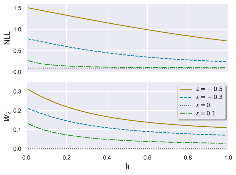
Figure 3: (Top) Negative log-likelihood (NLL) of the 1-dim. Gaussian toy model. (Bottom) 2-Wasserstein metric ($W_{2}$) between the data distribution and the distribution obtained by the same model. Both panels are plotted as a function of parameter $\mathfrak{h}$.

In Fig. 3 (Top), we plot the NLL, $-\mathbb{E}_{p_{0}}[\log q^{\mathfrak{h}}_{0}(x_{0})]$, as a function of parameter $\mathfrak{h}$. Different lines correspond to different values of $\epsilon$. The NLL is computed analytically, and we give the details in Appendix C. For nonzero $\epsilon$, the score estimation is imperfect and the model distribution $q^{\mathfrak{h}}_{0}(x_{0})$ differs from the data distribution. In these situations at $\epsilon\neq 0$, the NLL acquires nontrivial dependence on $\mathfrak{h}$, meaning that the quality of generated images depends the noise level in the sampling process. In Fig. 3 (Top), the NLLs are decreasing functions of $\mathfrak{h}$, and the presence of noise improves the output quality. Depending on the choice of $\epsilon$, the NLL could be an increasing function of $\mathfrak{h}$ as well. For reference, in Fig. 3 (Bottom), we plot the 2-Wasserstein distance, $W_{2}$, between the data distribution and $q^{\mathfrak{h}}_{0}(x_{0})$ for different values of $\epsilon$. The qualitative behavior is consistent with that of the NLL.

5.2 Experiment of 2-dim. synthetic data

Let us show some examples of log-likelihood computation for noisy generating process with pre-trained diffusion models trained by two-dimensional (2-dim.) synthetic distributions, Swiss-roll and 25-Gaussian (see Sec. D.1).

Pretrained models

We train simple neural network: $\mathbf{(}\mathbf{x},t)\to{\tt concat}([\mathbf{x},t])\to\big{(}{\tt Dense}(128)\to{\tt swish}\big{)}^{3}\to{\tt Dense}(2)\to{\bm{s}}_{\theta}(\mathbf{x},t)$ by choosing one of the following SDE schedulings:

simple:

$\scriptsize\bm{f}(\mathbf{x},t)=-\frac{\beta}{2}t\mathbf{x},\quad g(t)=\sqrt{\beta t},\quad(\beta=20)$

cosine:

$\scriptsize\bm{f}(\mathbf{x},t)=-\frac{\pi}{2}\tan(\frac{\pi}{2}t)\mathbf{x},\quad g(t)=\sqrt{\pi\tan(\frac{\pi}{2}t)},\normalsize$

with time interval $t\in[T_{\text{min}},T_{\text{max}}]$, where $T_{\text{min}}\in\mathbb{R}$ is small but nonzero to avoid singular behavior around $t=0$. We take $T_{\text{min}}=0.01,\,T_{\text{max}}=1$ here. We train each model by using the following loss function:

$$\frac{1}{N_{\text{batch}}}\sum_{i=1}^{N_{\text{batch}}}\frac{g(t_{i})^{2}}{2}\left\|\frac{\mathbf{x}_{i,t}-\alpha(t_{i})\mathbf{x}_{i}}{\sigma(t_{i})^{2}}+{\bm{s}}_{\theta}(\mathbf{x}_{i,t},t_{i})\right\|^{2},$$ (18)

where the signal and noise functions $\alpha(t)$ and $\sigma(t)$ are fixed by the chosen SDE scheduling, and $t_{i}$ represents discretized time. To compute the above, we take the Monte-Carlo sampling with $N_{\text{batch}}$ batches of data according to $\mathbf{x}_{i,t}\sim\mathcal{N}(\alpha(t_{i})\mathbf{x}_{i},\sigma(t_{i})^{2}I)$. For more details about pretraining with explicit forms of $\alpha(t)$, $\sigma(t)$, $t_{i}$, and $N_{\text{batch}}$, see explanations around Eq. 108 in Sec. D.2.

NLL calculation

Our basic strategy is based on Theorem 4.2, the perturbative expansion of the log-likelihood with respect to the parameter $\mathfrak{h}$. To calculate the $O(\mathfrak{h})$ correction, we need the values of $\log q^{\mathfrak{h}=0}_{t}(\mathbf{x})$ and its derivatives. We can obtain $\log q^{\mathfrak{h}=0}_{t}(\mathbf{x})$ by solving the probability flow ODE; however, there is no closed formula for its derivatives. In this experiment, the dimension of $\mathbf{x}=[x,y]^{\top}$ is 2, and this relatively low dimensionality allows us to approximate derivatives by discretized differential operators with small $\Delta x$:

$$\hat{\nabla}\log q^{\mathfrak{h}=0}_{t}(\mathbf{x})$$

$$=\left[\begin{array}[]{l}\frac{\log q^{\mathfrak{h}=0}_{t}(\mathbf{x}_{t}+[\Delta x,0]^{\top})-\log q^{\mathfrak{h}=0}_{t}(\mathbf{x}_{t}-[\Delta x,0]^{\top})}{2\Delta x}\\ \frac{\log q^{\mathfrak{h}=0}_{t}(\mathbf{x}_{t}+[0,\Delta x]^{\top})-\log q^{\mathfrak{h}=0}_{t}(\mathbf{x}_{t}-[0,\Delta x]^{\top})}{2\Delta x}\end{array}\right],$$ (21)

$$\hat{\nabla}^{2}\log q^{\mathfrak{h}=0}_{t}(\mathbf{x})$$

$$=\Big{(}\log q^{\mathfrak{h}=0}_{t}(\mathbf{x}_{t}+[\Delta x,0]^{\top})+\log q^{\mathfrak{h}=0}_{t}(\mathbf{x}_{t}-[\Delta x,0]^{\top})$$

$$\quad+\log q^{\mathfrak{h}=0}_{t}(\mathbf{x}_{t}+[0,\Delta x]^{\top})+\log q^{\mathfrak{h}=0}_{t}(\mathbf{x}_{t}-[0,\Delta x]^{\top})$$

$$\quad-4\log q^{\mathfrak{h}=0}_{t}(\mathbf{x}_{t})\Big{)}/\Delta x^{2}.$$ (22)

There are inherent discretization errors that we need to carefully evaluate. More on this will be addressed later in our analysis.

Consequently, to obtain the $O(\mathfrak{h}^{1})$ correction, we need to evaluate a nested integral. The pseudocode detailing our calculation method is presented in Algorithm 1. We use scipy.integrate.solve_ivp (Virtanen et al., 2020) both in 0th-logqSolver and discrete-time update in 1th-logqSolver. We take $T_{\text{min}}>0$ as the initial time and $T_{\text{max}}$ as the terminal time for probability flow ODE. This amounts to calculating the NLL for generation by SDE (9) in time interval $[T_{\text{min}},T_{\text{max}}]$, and does not affect the sampling quality if we take sufficiently small $T_{\text{min}}$. We show our results in Table 1.

Algorithm 1 1st-logqSolver

  Input: data $\mathbf{x}$, small $\Delta x$, SDE info $[{\bm{f}}(\cdot,t),g(t),T_{\text{min}},T_{\text{max}}]$, solver 0th-logqSolver

  Initialize: $t=T_{\text{min}}$, $\mathbf{x}_{t}=\mathbf{x}$, $\delta\mathbf{x}_{t}=\mathbf{0}$, $\delta\log q_{t}=0$

  Calculate $\log q_{0}\leftarrow$ 0th-logqSolver($\mathbf{x},t=T_{\text{min}}$)

  repeat

     Calculate

$$\log q_{t} \leftarrow\text{\tt 0th-logqSolver}(\mathbf{x}_{t},t)$$

$$\log q_{t}^{x+} \leftarrow\text{\tt 0th-logqSolver}(\mathbf{x}_{t}+[\Delta x,0]^{\top},t)$$

$$\log q_{t}^{x-} \leftarrow\text{\tt 0th-logqSolver}(\mathbf{x}_{t}-[\Delta x,0]^{\top},t)$$

$$\log q_{t}^{y+} \leftarrow\text{\tt 0th-logqSolver}(\mathbf{x}_{t}+[0,\Delta x]^{\top},t)$$

$$\log q_{t}^{y-} \leftarrow\text{\tt 0th-logqSolver}(\mathbf{x}_{t}-[0,\Delta x]^{\top},t)$$

     Calculate $\bm{f}^{\rm PF}_{\theta}(\mathbf{x}_{t},t)$

     Calculate $\delta{\bm{f}}^{\rm PF}_{\theta}(\mathbf{x}_{t},\delta\mathbf{x}_{t},t)$ by $\log q_{t}^{x/y\pm}$ and (21)

     Calculate $\nabla\cdot\delta{\bm{f}}^{\rm PF}_{\theta}(\mathbf{x}_{t},\delta\mathbf{x}_{t},t)$ by $\log q_{t}^{x/y\pm}$ and (22)

     Update $t,\mathbf{x}_{t},\delta\mathbf{x}_{t},\delta\log q_{t}$ by time-discretized version (e.g. Runge-Kutta update) based on

$$\dot{\mathbf{x}}_{t} =\bm{f}^{\rm PF}_{\theta}(\mathbf{x}_{t},t)$$

$$\dot{\delta\mathbf{x}}_{t} =\delta{\bm{f}}^{\rm PF}_{\theta}(\mathbf{x}_{t},\delta\mathbf{x}_{t},t)$$

$$\dot{\delta\log q_{t}} =\nabla\cdot\delta{\bm{f}}^{\rm PF}_{\theta}(\mathbf{x}_{t},\delta\mathbf{x}_{t},t)$$

  until $t=T_{\text{max}}$

  $\text{1st-correction}=\delta\mathbf{x}_{T}\cdot\nabla\log\pi(\mathbf{x}_{T})+\delta\log q_{T}$

  Output: $\log q_{0},\text{1st-correction}$

Numerical errors

In Algorithm 1, we made two approximations in discrete differential operators and ODE solvers. To ensure reliability of our results, it is essential to assess and estimate the associated errors. Let us call the numerical value of $\log q^{\mathfrak{h}=0}_{t}(\mathbf{x})$ calculated by 0th-logqSolver in Algorithm 1 as $N[\log q^{\mathfrak{h}=0}_{t}(\mathbf{x})]$, then we have two local errors:

$$\small\begin{split}\text{err}\bigl{(}\hat{\nabla}N[\log q^{\mathfrak{h}=0}_{t}(\mathbf{x})]\bigr{)}&=\nabla\log q^{\mathfrak{h}=0}_{t}(\mathbf{x})\!-\!\hat{\nabla}N[\log q^{\mathfrak{h}=0}_{t}(\mathbf{x})],\\ \text{err}\bigl{(}\hat{\nabla}^{2}N[\log q^{\mathfrak{h}=0}_{t}(\mathbf{x})]\bigr{)}&=\nabla^{2}\log q^{\mathfrak{h}=0}_{t}(\mathbf{x})\!-\!\hat{\nabla}^{2}N[\log q^{\mathfrak{h}=0}_{t}(\mathbf{x})].\end{split}$$ (23)

Exact calculation of these values is unachievable, and nevertheless, we should somehow estimate them. We propose two estimation schemes, subtraction (Sec. E.2) and model (Sec. E.3). Here, we show results based on the latter method, which operates at a higher speed. In addition, we should integrate these local errors to estimate the error piled up in the final results. This can also be calculated numerically by the ODE solver, and the numerical errors estimated in this way are shown in Table 1. See Appendix E for more details.

Comparison to 2-Wasserstein

We also show 2-Wasserstein distance, $W_{2}$, between validation data and generated data in Fig. 4 with stochastic SDE (9). We see that the $W_{2}$ values typically decrease especially in the small $\mathfrak{h}$ region, which signifies the improvement of generated data quality. This observation is consistent with negative-valued NLL corrections in 1st-corr column in Table 1. The overall trend is the same as the results from the analytical study in Sec. 5.1; the tendency of enhancing sampled data quality by noise has been confirmed by our experiment even in intricate cases where exact calculation is not accessible. In addition, considering that the values in 1st-corr column are the first-order derivative of NLL (cross-entropy) with respect to $\mathfrak{h}$, one might say that the values for cosine-SDE are a few times larger than the values for simple-SDE, which agrees with the behavior of the first-order derivative near $\mathfrak{h}=0$ in Fig. 4.

Table 1: NLL (cross-entropy) and its $O(\mathfrak{h}^{1})$ corrections. We apply $\Delta x$ = 0.01 to compute (21) and (22). tol represents the value of absolute and relative tolerances of updates in Algorithm 1. We set absolute and relative tolerances of 0th-logqSolver as order 1e-5.

Swiss-roll
SDE (NLL)	tol	1st-corr	errors
simple (1.39$\pm$ 0.05)	1e-3	-0.31$\pm$0.21	0.13$\pm$0.00
	1e-5	-0.44$\pm$0.38	0.13$\pm$0.00
cosine (1.42$\pm$ 0.02)	1e-3	-1.59$\pm$0.57	0.35$\pm$0.00
	1e-5	-3.27$\pm$1.11	0.37$\pm$0.02
25-gaussian
SDE (NLL)	tol	1st-corr	errors
simple (-1.22$\pm$ 0.01)	1e-3	-3.64$\pm$0.49	0.31$\pm$0.00
	1e-5	-3.61$\pm$0.64	0.32$\pm$0.01
cosine (-1.71$\pm$ 0.02)	1e-3	-17.57$\pm$5.56	0.70$\pm$0.01
	1e-5	-19.65$\pm$17.46	0.67$\pm$0.03

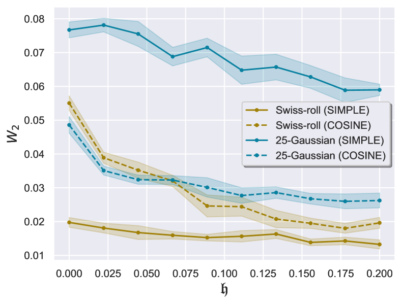
Figure 4: 2-Wasserstein metrics ($W_{2}$) by POT library (Flamary et al., 2021) between validation data and generated data via (9) with Swiss-roll data and 25-Gaussian data with SIMPLE and COSINE SDE scheduling. The dots and the errorbars represent the mean values over 10 independent trials and $\pm$std$/\sqrt{10}$, respectively.

6 Conclusions

We presented a novel formulation of diffusion models utilizing the path integral framework, originally developed in quantum physics. This formulation provides a unified perspective on various aspects of score-based generative models, and we gave the re-derivation of reverse-time SDEs and loss functions for training. In particular, one can introduce a continuous parameter linking different sampling schemes: the probability flow ODEs and stochastic generation. We have performed the expansion with respect to this parameter and perturbatively evaluated the negative log-likelihood, which is a reminiscent of the WKB expansion in quantum physics. In this way, this formulation has presented a new method for scrutinizing the role of noise in the sampling process.

An interesting future direction is an extension of the analysis based on path integral formalism for diffusion Schrödinger bridges (De Bortoli et al., 2021), in which the prior can be more general. Another direction is to understand the cases mentioned in (Karras et al., 2022), where injecting noise would rather degrade the quality of the generated data. This is an open problem, and there is room for deeper study in terms of log-likelihood calculations based on WKB expansions.

Limitations

Our experiments did not involve actual image data. This omission is primarily due to the current evaluation method’s limitations regarding NLLs, which are not directly applicable to high-dimensional data such as images on account of the uses of explicit discrete differentials. Another limitation is the potential of underestimated numerical error in our computed NLLs. Although our estimated local errors look safe (Sec. E.5), they are potentially underestimated because the estimation is based on score-based model that does not match to $\nabla\log q_{t}(\mathbf{x})$ exactly in general.

Appendix A From SDE to path integral

In this appendix, we describe the details of the path integral formulation of diffusion models.

A.1 Discretization schemes

In later discussions, we will introduce discretized summations in different ways, which do not seem apparent in their continuum counterpart. We here introduce discretization schemes that will be used in later analyses.

Suppose we have $\{\mathbf{x}_{t}\}_{t\in[0,T]}$ obeying SDE (1). We discretize the time interval $[0,T]$ with width $\Delta t$ and $M\coloneqq T/\Delta t$, which we take to be an integer. Let us take the following summation:

$$\sum_{n=0}^{M-1}\bm{f}_{t_{n}}\cdot(\mathbf{x}_{{t_{n}}+\Delta t}-\mathbf{x}_{t_{n}}),$$ (24)

where $t_{n}\coloneqq n\Delta t$ and $\bm{f}_{t}=\bm{f}(\mathbf{x}_{t},t)$. We will consider the continuum limit $\Delta t\to 0$ and will refer to this as the Itô scheme, which will be denoted by

$$\int\bm{f}\cdot{\rm d}\mathbf{x}\coloneqq\int\bm{f}_{t}\cdot(\mathbf{x}_{t+{\rm d}t}-\mathbf{x}_{t}).$$ (25)

A common prescription in the physics literature is the Stratonovich scheme,

$$\int\bm{f}\circ{\rm d}\mathbf{x}\coloneqq\int\frac{\bm{f}_{t}+\bm{f}_{t+{\rm d}t}}{2}\cdot(\mathbf{x}_{t+{\rm d}t}-\mathbf{x}_{t}),$$ (26)

which should be understood as a short-hand notation for the following equation,

$$\lim_{\Delta t\to 0}\sum_{n=0}^{M-1}\frac{\bm{f}_{t_{n}}+\bm{f}_{t_{n}+\Delta t}}{2}\cdot(\mathbf{x}_{{t_{n}}+\Delta t}-\mathbf{x}_{t_{n}}).$$ (27)

We also encounter the reverse-Itô scheme, which is written as

$$\int\bm{f}\,\tilde{\cdot}\,{\rm d}\mathbf{x}\coloneqq\int\bm{f}(\mathbf{x}_{t+{\rm d}t})\cdot(\mathbf{x}_{t+{\rm d}t}-\mathbf{x}_{t}).$$ (28)

This can be seen as the Itô scheme in reverse time.

A.2 Derivation of the path integral expression

Here, we give a derivation of the path integral representation of a diffusion model (Proposition 3.1). We consider a forward process described by the SDE (1). In the physics literature, Eq. (1) is commonly expressed in the following form,

$$\quad\dot{\mathbf{x}}_{t}=\bm{f}(\mathbf{x}_{t},t)+\bm{\xi}_{t},$$ (29)

where the noise term satisfies

$$\mathbb{E}[\xi^{i}_{t}\xi^{j}_{t^{\prime}}]=g(t)^{2}\delta^{ij}\delta(t-t^{\prime}).$$ (30)

The expectation value of a generic observable $\mathcal{O}(\{\mathbf{x}_{t}\})$ over noise realizations can be expressed as

$$\mathbb{E}_{P[\{\mathbf{x}_{t}\}]}[\mathcal{O}(\{\mathbf{x}_{t}\})]=\int[D\mathbf{x}_{t}][D\bm{\xi}_{t}]\,\mathcal{O}(\{\mathbf{x}_{t}\})\left(\prod_{t}\delta(\mathbf{x}_{t}-\mathbf{x}^{\rm sol}_{t})\right)e^{-\int_{0}^{T}\frac{1}{2g(t)^{2}}\|\bm{\xi}_{t}\|^{2}{\rm d}t}p_{0}(\mathbf{x}_{0}),$$ (31)

where $p_{0}(\mathbf{x}_{0})$ is the probability distribution of initial states (i.e., the data distribution), $\delta(\cdot)$ is Dirac’s delta function, and $\mathbf{x}^{\rm sol}_{t}$ is the solution of Eq. (29). The symbol $[D\mathbf{x}_{t}]_{\Delta t}$ denotes $[D\mathbf{x}_{t}]_{\Delta t}\coloneqq\prod_{n=0}^{M}C(\Delta t){\rm d}\mathbf{x}_{t_{n}}$, where $C(\Delta t)$ is a normalization constant, and similarly for $[D\bm{\xi}_{t}]$. When the weight is sufficiently well-behaved (like $e^{-\int_{0}^{T}\frac{1}{2g(t)^{2}}\|\bm{\xi}_{t}\|^{2}{\rm d}t}$ in Eq. 31), the limit $\Delta t\to 0$ the path integral is well-defined. We will be considering this limit at the end of the calculation do not explicitly indicate the dependence on $\Delta t$ hereafter. The delta function imposes that $\mathbf{x}_{t}$ is a solution of Eq. (29) under a given noise realization. Using the change-of-variable formula for the delta function,

$$\delta(\mathbf{x}_{t}-\mathbf{x}^{\rm sol}_{t})=\left|\det\frac{\delta{\rm EOM}_{t}}{\delta\mathbf{x}_{t^{\prime}}}\right|\delta({\rm EOM}_{t}),$$ (32)

where ${\rm EOM}_{t}\coloneqq\dot{\mathbf{x}}_{t}-\bm{f}(\mathbf{x}_{t},t)-\bm{\xi}_{t}$. The Jacobian part gives a nontrivial contribution (see Appendix B for a detailed derivation) in the case of the Stratonovich scheme,

$$\begin{split}\left|\det\frac{\delta{\rm EOM}_{t}}{\delta\mathbf{x}_{t^{\prime}}}\right|&=\det(\partial_{t}\delta_{ij}-\partial_{i}f_{j})\\ &=\det\partial_{t}\,\det(\delta_{ij}-\partial_{t}^{-1}\partial_{i}f_{j})\\ &\propto e^{-\frac{1}{2}\int\nabla\cdot\bm{f}(\mathbf{x}_{t},t){\rm d}t},\end{split}$$ (33)

while it gives a trivial factor for the Itô scheme. Writing this factor as $e^{-J}$, the expectation value can now be written as

$$\mathbb{E}_{P[\{\mathbf{x}_{t}\}]}[\mathcal{O}(\{\mathbf{x}_{t}\})]=\int[D\mathbf{x}_{t}][D\bm{\xi}_{t}]\,\mathcal{O}(\{\mathbf{x}_{t}\})e^{-J}\left(\prod_{t}\delta(\dot{\mathbf{x}}_{t}-\bm{f}_{t}-\bm{\xi}_{t})\right)e^{-\int_{0}^{T}\frac{1}{2g(t)^{2}}\|\bm{\xi}_{t}\|^{2}{\rm d}t}p_{0}(\mathbf{x}_{0}).$$ (34)

Performing the integration over $\bm{\xi}_{t}$, we arrive at the expression

$$\mathbb{E}_{P[\{\mathbf{x}_{t}\}]}[\mathcal{O}(\{\mathbf{x}_{t}\})]=\int[D\mathbf{x}_{t}]\,\mathcal{O}(\{\mathbf{x}_{t}\})\,e^{-\mathcal{A}}p_{0}(\mathbf{x}_{0}),$$ (35)

Here, we defined the action $\mathcal{A}$ by

$$\mathcal{A}\coloneqq\int_{0}^{T}L(\dot{\mathbf{x}}_{t},\mathbf{x}_{t}){\rm d}t+J$$ (36)

where $L(\dot{\mathbf{x}}_{t},\mathbf{x}_{t})$ is the Onsager-Machlup function  (Onsager & Machlup, 1953; Machlup & Onsager, 1953) given by

$$L(\dot{\mathbf{x}}_{t},\mathbf{x}_{t})=\frac{1}{2g(t)^{2}}\|\dot{\mathbf{x}}_{t}-\bm{f}(\mathbf{x}_{t},t)\|^{2},$$ (37)

and $J$ is the term coming from the Jacobian, which depends on the choice of the discretization scheme:

$$J=\begin{cases}0&\text{It\^{o}}\\ \int_{0}^{T}\frac{1}{2}\nabla\cdot\bm{f}_{t}(\mathbf{x}_{t},t){\rm d}t&\text{Stratonovich}\\ \int_{0}^{T}\nabla\cdot\bm{f}_{t}(\mathbf{x}_{t},t){\rm d}t&\text{Reverse-It\^{o}}\end{cases}.$$ (38)

This concludes the derivation of Proposition 3.1. Any observable can be computed using the weight given by $\mathcal{A}$. For example, one can compute the joint probability for the variables on discrete time points $\{t_{n}\}_{n=1,\ldots,N}$ as

$$P(\mathbf{y}_{t_{1}},\mathbf{y}_{t_{2}},\ldots,\mathbf{y}_{t_{N}})=\int[D\mathbf{x}_{t}]\,e^{-\mathcal{A}}\,p_{0}(\mathbf{x}_{0})\,\prod_{n=1}^{N}\delta(\mathbf{y}_{t_{n}}-\mathbf{x}_{t_{n}}).$$ (39)

A.3 Time-reversed SDE

Here we present the derivation of the time-reversed dynamics in the path integral formalism (Proposition 3.2). We will use the Itô scheme, and later comment on other discretization schemes. We start by rewriting Eq. (35) as

$$\begin{split}\mathbb{E}_{P[\{\mathbf{x}_{t}\}]}[\mathcal{O}(\{\mathbf{x}_{t}\})]&=\int[D\mathbf{x}_{t}]\,\mathcal{O}(\{\mathbf{x}_{t}\})\,p_{T}(\mathbf{x}_{T})\,e^{\int_{0}^{T}[-L-\ln p_{T}(\mathbf{x}_{T})+\ln p_{0}(\mathbf{x}_{0})]{\rm d}t}\\ &=\int[D\mathbf{x}_{t}]\,p_{T}(\mathbf{x}_{T})\,e^{-\widetilde{\mathcal{A}}},\end{split}$$ (40)

where $\widetilde{\mathcal{A}}\coloneqq\int_{0}^{T}\widetilde{L}(\dot{\mathbf{x}}_{t},\mathbf{x}_{t}){\rm d}t$ with

$$\widetilde{L}(\dot{\mathbf{x}}_{t},\mathbf{x}_{t})\coloneqq L(\dot{\mathbf{x}}_{t},\mathbf{x}_{t})+\frac{{\rm d}}{{\rm d}t}\ln p_{t}(\mathbf{x}_{t}).$$ (41)

The total time derivative of $\ln p_{t}(\mathbf{x}_{t})$ is written as

$${\rm d}\ln p_{t}(\mathbf{x}_{t})=\partial_{t}\ln p_{t}(\mathbf{x}_{t}){\rm d}t+{\rm d}\mathbf{x}_{t}\cdot\nabla\ln p_{t}(\mathbf{x}_{t})+\frac{1}{2}g(t)^{2}\nabla^{2}\ln p_{t}(\mathbf{x}_{t}){\rm d}t,$$ (42)

where we have used Itô’s formula. For $\partial_{t}p_{t}(\mathbf{x}_{t})$, we use the Fokker-Planck equation,

$$\partial_{t}p_{t}(\mathbf{x})=-\nabla\cdot\left(\bm{f}(\mathbf{x}_{t},t)p_{t}(\mathbf{x})-\frac{g(t)^{2}}{2}\nabla p_{t}(\mathbf{x})\right),$$ (43)

which we rewrite as

$$\partial_{t}\ln p_{t}(\mathbf{x})=-\nabla\cdot\bm{f}(\mathbf{x}_{t},t)-\bm{f}(\mathbf{x}_{t},t)\cdot\nabla\ln p_{t}(\mathbf{x})+\frac{g(t)^{2}}{2}\left[\nabla^{2}\ln p_{t}(\mathbf{x})+(\nabla\ln p_{t}(\mathbf{x}))^{2}\right].$$ (44)

The new Lagrangian $\widetilde{L}(\dot{\mathbf{x}}_{t},\mathbf{x}_{t})$ is now written as

$$\begin{split}\widetilde{L}(\dot{\mathbf{x}}_{t},\mathbf{x}_{t})&=\frac{1}{2g_{t}^{2}}(\dot{\mathbf{x}}^{2}-2\dot{\mathbf{x}}\cdot(\bm{f}(\mathbf{x}_{t},t)-g(t)^{2}\nabla\ln p_{t}(\mathbf{x}_{t}))+\bm{f}(\mathbf{x}_{t},t)^{2})+\frac{g(t)^{2}}{2}\nabla^{2}\ln p_{t}(\mathbf{x}_{t})\\ &\quad-\nabla\cdot\bm{f}(\mathbf{x}_{t},t)-\bm{f}(\mathbf{x}_{t},t)\cdot\nabla\ln p_{t}(\mathbf{x}_{t})+\frac{g(t)^{2}}{2}\left[\nabla^{2}\ln p_{t}(\mathbf{x}_{t})+(\nabla\ln p_{t}(\mathbf{x}_{t}))^{2}\right]\\ &=\frac{1}{2g_{t}^{2}}(\dot{\mathbf{x}}-\bm{f}(\mathbf{x}_{t},t)+g(t)^{2}\nabla\ln p_{t}(\mathbf{x}_{t}))^{2}-\nabla\cdot\left(\bm{f}(\mathbf{x}_{t},t)-g(t)^{2}\nabla\ln p_{t}(\mathbf{x}_{t})\right).\end{split}$$ (45)

Thus, the action $\widetilde{\mathcal{A}}$ is given by

$$\int_{0}^{T}\widetilde{L}(\dot{\mathbf{x}}_{t},\mathbf{x}_{t}){\rm d}t=\int_{0}^{T}\left[\frac{1}{2g(t)^{2}}\|\dot{\mathbf{x}}_{t}-\widetilde{\bm{f}}(\mathbf{x}_{t},t)\|^{2}-\nabla\cdot\widetilde{\bm{f}}(\mathbf{x}_{t},t)\right]{\rm d}t,$$ (46)

where

$$\widetilde{\bm{f}}(\mathbf{x}_{t},t)\coloneqq\bm{f}(\mathbf{x}_{t},t)-g(t)^{2}\nabla\ln p_{t}(\mathbf{x}_{t}).$$ (47)

Note that there appears a nontrivial Jacobian term in Eq. (46). This term disappears if we rewrite the integral using the inverse time $\tau$ in the Itô convention. The action $\widetilde{\mathcal{A}}$ contains the following contribution,

$$\widetilde{\mathcal{A}}\supset-\int\frac{1}{g(t)^{2}}\widetilde{\bm{f}}(\mathbf{x}_{t},t)\cdot{\rm d}\mathbf{x}_{t}.$$ (48)

Currently, this product written in the Itô scheme. We rewrite this term in the reverse-Itô scheme,

$$\begin{split}\widetilde{\bm{f}}_{t}\cdot{\rm d}\mathbf{x}_{t}&=\left[\widetilde{\bm{f}}_{t+{\rm d}t}-\left(\widetilde{\bm{f}}_{t+{\rm d}t}-\widetilde{\bm{f}}_{t}\right)\right]\cdot{\rm d}\mathbf{x}_{t}=\widetilde{\bm{f}}_{t+{\rm d}t}\cdot{\rm d}\mathbf{x}_{t}-\sum_{i,j}\partial_{i}(\widetilde{f}_{t})_{j}{\rm d}x_{i}{\rm d}x_{j}\\ &=\widetilde{\bm{f}}_{t+{\rm d}t}\cdot{\rm d}\mathbf{x}_{t}-g(t)^{2}\nabla\cdot\widetilde{\bm{f}}_{t}\,{\rm d}t.\end{split}$$ (49)

The second term of this equation cancels the Jacobian term. Thus, the time-reversed action can be naturally interpreted as an Itô integral in reverse time.

The same procedure can be also done for the Stratonovich scheme. The difference is the presence of the Jacobian term in the original action and the total time derivative of $p_{t}(\mathbf{x}_{t})$ is written as

$${\rm d}\ln p_{t}(\mathbf{x}_{t})=\partial_{t}\ln p_{t}(\mathbf{x}_{t}){\rm d}t+{\rm d}\mathbf{x}_{t}\cdot\nabla\ln p_{t}(\mathbf{x}_{t})$$ (50)

instead of Eq. (42). Following similar steps, the time-reversed action is found to be given by

$$\widetilde{\mathcal{A}}=\int_{0}^{T}\widetilde{L}(\dot{\mathbf{x}}_{t},\mathbf{x}_{t}){\rm d}t=\int_{0}^{T}\left[\frac{1}{2g(t)^{2}}\|\dot{\mathbf{x}}_{t}-\widetilde{\bm{f}}_{t}\|^{2}-\frac{1}{2}\nabla\cdot\widetilde{\bm{f}}_{t}\right]{\rm d}t.$$ (51)

Note that the sign of the Jacobian term is flipped compared with the original action, which allows us to interpret the process as a time-reversed one.

A.4 Evaluation of KL divergence

We here give the derivation of Proposition 3.3. We evaluate the upper limit of the KL divergence of the data distribution and a model,

$$D_{\rm KL}(p_{0}(\mathbf{x}_{0})\|q_{0}(\mathbf{x}_{0}))\leq D_{\rm KL}(P(\{\mathbf{x}_{t}\}_{t\in[0,T]})\|Q(\{\mathbf{x}_{t}\}_{t\in[0,T]})),$$ (52)

where we used the data processing inequality. Below, we evaluate the RHS of Eq. 52.

The time-reversed action of the data distribution (in the reverse-Itô scheme) reads

$$\widetilde{\mathcal{A}}\coloneqq\int_{0}^{T}\widetilde{L}(\dot{\mathbf{x}}_{t},\mathbf{x}_{t}){\rm d}t=\int_{0}^{T}\left[\frac{1}{2g(t)^{2}}\|\dot{\mathbf{x}}_{t}-\widetilde{\bm{f}}(\mathbf{x}_{t},t)\|^{2}\right]{\rm d}t,$$ (53)

The time-reversed action of a model is given by

$$\widetilde{\mathcal{A}}_{\theta}\coloneqq\int_{0}^{T}\widetilde{L}_{\theta}(\dot{\mathbf{x}}_{t},\mathbf{x}_{t}){\rm d}t=\int_{0}^{T}\left[\frac{1}{2g(t)^{2}}\|\dot{\mathbf{x}}_{t}-\widetilde{\bm{f}}_{\theta}(\mathbf{x}_{t},t)\|^{2}\right]{\rm d}t,$$ (54)

with

$$\widetilde{\bm{f}}_{\theta}(\mathbf{x}_{t},t)\coloneqq\bm{f}(\mathbf{x}_{t},t)-g(t)^{2}\bm{s}_{\theta}(\mathbf{x}_{t},t).$$ (55)

We note that, we employ the reverse-Itô scheme in the following computation and that is why there is no Jacobian term in Eqs. 53 and 54. We rewrite the joint probability of paths as

$$P(\{\mathbf{x}_{t}\}_{t\in[0,T]}) =e^{-\mathcal{A}}p_{0}(\mathbf{x}_{0})=p_{T}(\mathbf{x}_{T})e^{-\widetilde{\mathcal{A}}},$$ (56)

$$Q(\{\mathbf{x}_{t}\}_{t\in[0,T]}) =e^{-\mathcal{A}_{\theta}}q_{0}(\mathbf{x}_{0})=q_{T}(\mathbf{x}_{T})e^{-\widetilde{\mathcal{A}}_{\theta}}.$$ (57)

The KL divergence of the path-probability $P(\{\mathbf{x}_{t}\}_{t})$ from $Q(\{\mathbf{x}_{t}\}_{t})$ is written as

$$\begin{split}D_{\rm KL}\left(P(\{\mathbf{x}_{t}\}_{t\in[0,T]})\|Q(\{\mathbf{x}_{t}\}_{t\in[0,T]})\right)&=\mathbb{E}_{P(\{\mathbf{x}_{t}\})}\left[\ln\frac{P(\{\mathbf{x}_{t}\}_{t\in[0,T]})}{Q(\{\mathbf{x}_{t}\}_{t\in[0,T]})}\right]\\ &=\mathbb{E}_{P(\{\mathbf{x}_{t}\}_{t})}\left[\ln\frac{p_{T}(\mathbf{x}_{T})}{q_{T}(\mathbf{x}_{T})}-\widetilde{\mathcal{A}}+\widetilde{\mathcal{A}}_{\theta}\right]\\ &=D_{\rm KL}\left(p_{T}(\mathbf{x}_{T})\|q_{T}(\mathbf{x}_{T})\right)+\mathbb{E}_{P(\{\mathbf{x}_{t}\}_{t})}\left[\widetilde{\mathcal{A}}_{\theta}-\widetilde{\mathcal{A}}\right].\end{split}$$ (58)

The second term of the RHS can be written as

$$\begin{split}\mathbb{E}_{P(\{\mathbf{x}_{t}\}_{t})}\left[\widetilde{\mathcal{A}}_{\theta}-\widetilde{\mathcal{A}}\right]&=\mathbb{E}_{P(\{\mathbf{x}_{t}\}_{t})}\int_{0}^{T}\frac{1}{2g(t)^{2}}\left[-2\dot{\mathbf{x}}_{t}\tilde{\cdot}(\widetilde{\bm{f}}_{\theta}(\mathbf{x}_{t},t)-\widetilde{\bm{f}}(\mathbf{x}_{t},t))+(\widetilde{\bm{f}}_{\theta}(\mathbf{x}_{t},t))^{2}-(\widetilde{\bm{f}}(\mathbf{x}_{t},t))^{2}\right]{\rm d}t\\ &=\mathbb{E}_{P(\{\mathbf{x}_{t}\}_{t})}\int_{0}^{T}\frac{1}{2g(t)^{2}}[\widetilde{\bm{f}}_{\theta}(\mathbf{x}_{t+{\rm d}t},t+{\rm d}t)-\widetilde{\bm{f}}(\mathbf{x}_{t+{\rm d}t},t+{\rm d}t)]\cdot[-2\dot{\mathbf{x}}_{t}+\widetilde{\bm{f}}_{\theta}(\mathbf{x}_{t},t)+\widetilde{\bm{f}}(\mathbf{x}_{t},t)]{\rm d}t.\end{split}$$ (59)

We discretize this and look at the contribution from the neighboring part $(t,t+\Delta t)$,

$$\begin{split}&\mathbb{E}_{P(\mathbf{x}_{t},\mathbf{x}_{t+\Delta t})}\left[\Delta t\,\frac{1}{2g(t)^{2}}(\widetilde{\bm{f}}_{\theta,t+\Delta t}-\widetilde{\bm{f}}_{t+\Delta t})\cdot\left[-2(\mathbf{x}_{t+\Delta t}-\mathbf{x}_{t})/\Delta t+\widetilde{\bm{f}}_{\theta,t}+\widetilde{\bm{f}}_{t}\right]\right]\\ &=\mathbb{E}_{p_{t}(\mathbf{x}_{t})}\left[\Delta t\,\frac{1}{2g(t)^{2}}(\widetilde{\bm{f}}_{\theta,t+\Delta t}-\widetilde{\bm{f}}_{t+\Delta t})\cdot(-2\widetilde{\bm{f}}_{t}+\widetilde{\bm{f}}_{\theta,t}+\widetilde{\bm{f}}_{t})\right]\\ &=\mathbb{E}_{p_{t}(\mathbf{x}_{t})}\left[\Delta t\,\frac{1}{2g(t)^{2}}\|\widetilde{\bm{f}}_{\theta,t}-\widetilde{\bm{f}}_{t}\|^{2}+O(\Delta t^{2})\right],\end{split}$$ (60)

where we performed the summation over $\mathbf{\delta}=\mathbf{x}_{t+\Delta t}-\mathbf{x}_{t}$. Summing up these contributions for $[0,T]$, we have

$$\begin{split}\mathbb{E}_{P(\{\mathbf{x}_{t}\}_{t})}\left[\widetilde{\mathcal{A}}_{\theta}-\widetilde{\mathcal{A}}\right]&=\mathbb{E}_{P(\{\mathbf{x}_{t}\}_{t})}\left[\int_{0}^{T}\frac{1}{2g(t)^{2}}\|\widetilde{\bm{f}}_{\theta}(\mathbf{x}_{t},t)-\widetilde{\bm{f}}(\mathbf{x}_{t},t)\|^{2}{\rm d}t\right]\\ &=\mathbb{E}_{P(\{\mathbf{x}_{t}\}_{t})}\left[\int_{0}^{T}\frac{g(t)^{2}}{2}\|\nabla\ln p_{t}(\mathbf{x}_{t})-\bm{s}_{\theta}(\mathbf{x}_{t},t)\|^{2}{\rm d}t\right].\end{split}$$ (61)

Thus, we have obtained the following inequality,

$$D_{\rm KL}(p_{0}(\mathbf{x}_{0})\|q_{0}(\mathbf{x}_{0}))\leq D_{\rm KL}\left(p_{T}(\mathbf{x}_{T})\|q_{T}(\mathbf{x}_{T})\right)+\int_{0}^{T}\frac{g(t)^{2}}{2}\mathbb{E}_{p_{t}}\left[\|\nabla\ln p_{t}(\mathbf{x}_{t})-\bm{s}_{\theta}(\mathbf{x}_{t},t)\|^{2}\right]{\rm d}t.$$ (62)

The distribution $q_{T}(\mathbf{x}_{T})$ is taken to be a prior, $\pi(\mathbf{x}_{T})$. This concludes the proof of Proposition 3.3.

A.5 Conditional variants

A similar argument applies to the case when the initial state is fixed. The derivation of the reverse process can be obtained by replacing the probability densities with conditional ones on a chosen initial state $\mathbf{x}^{\prime}_{0}$. The expectation value of a general observable in this situation can be written as

$$\mathbb{E}_{P(\{\mathbf{x}_{t}\}_{t\in(0,T]}|\mathbf{x}^{\prime}_{0})}[\mathcal{O}(\{\mathbf{x}_{t}\})]=\int[D\mathbf{x}_{t}]\,\mathcal{O}(\{\mathbf{x}_{t}\})\,e^{-\int L{\rm d}t}\delta(\mathbf{x}_{0}-\mathbf{x}^{\prime}_{0}).$$ (63)

Similarly to the previous section, we can rewrite this as

$$\begin{split}\mathbb{E}_{P(\{\mathbf{x}_{t}\}_{t\in(0,T]}|\mathbf{x}^{\prime}_{0})}[\mathcal{O}(\{\mathbf{x}_{t}\})]&=\int[D\mathbf{x}_{t}]\,\mathcal{O}(\{x_{t}\})\,P_{T}(\mathbf{x}_{T}|\mathbf{x}^{\prime}_{0})\,e^{-\widetilde{\mathcal{A}}(\mathbf{x}^{\prime}_{0})}\delta(\mathbf{x}_{0}-\mathbf{x}^{\prime}_{0}),\end{split}$$ (64)

where $\widetilde{\mathcal{A}}(\mathbf{x}^{\prime}_{0})\coloneqq\int_{0}^{T}\widetilde{L}(\dot{\mathbf{x}}_{t},\mathbf{x}_{t}|\mathbf{x}^{\prime}_{0})\,{\rm d}t$ with

$$\widetilde{L}(\dot{\mathbf{x}}_{t},\mathbf{x}_{t}|\mathbf{x}^{\prime}_{0})\coloneqq L(\dot{\mathbf{x}}_{t},\mathbf{x}_{t}|\mathbf{x}^{\prime}_{0})+\frac{{\rm d}}{{\rm d}t}p_{t}(\mathbf{x}_{t}|\mathbf{x}^{\prime}_{0}).$$ (65)

Following similar calculations with the unconditional case, the force of the reverse process turns out to be given by

$$\widetilde{\bm{f}}(\mathbf{x}_{t},t)\coloneqq\bm{f}(\mathbf{x}_{t},t)-g(t)^{2}\nabla\ln p_{t}(\mathbf{x}_{t}|\mathbf{x}^{\prime}_{0}).$$ (66)

One can also repeat a similar argument for the evaluation of the KL divergence with fixed $\mathbf{x}_{0}^{\prime}$, which corresponds to the ELBO-based loss (Kingma et al., 2021; Kingma & Gao, 2023):

Proposition A.1.

Let $p_{t}(\mathbf{x}|\mathbf{x}_{0})$ as the Markov kernel from time $0$ to $t$ determined by the Fokker-Planck equation. Determining the Onsager–Machlup function for reverse process $\widetilde{L}(\dot{\mathbf{x}}_{t},\mathbf{x}_{t}|\mathbf{x}_{0}^{\prime})$ to satisfy

$$p_{0}(\mathbf{x}_{0}|\mathbf{x}_{0}^{\prime})e^{-\int_{0}^{T}L(\dot{\mathbf{x}}_{t},\mathbf{x}_{t}){\rm d}t+J}[D\mathbf{x}_{t}]=e^{-\int_{0}^{T}\widetilde{L}(\dot{\mathbf{x}}_{t},\mathbf{x}_{t}|\mathbf{x}_{0}^{\prime}){\rm d}t+\widetilde{J}(\mathbf{x}_{0}^{\prime})}p_{T}(\mathbf{x}_{T}|\mathbf{x}_{0}^{\prime})[D\mathbf{x}_{t}],$$ (67)

yields

$$\widetilde{L}(\dot{\mathbf{x}}_{t},\mathbf{x}_{t}|\mathbf{x}_{0}^{\prime}) =\frac{\|\dot{\mathbf{x}}_{t}-\bm{f}(\mathbf{x}_{t},t)+g(t)^{2}\nabla\log p_{t}(\mathbf{x}_{t}|\mathbf{x}_{0}^{\prime})\|^{2}}{2g(t)^{2}},$$ (68)

where $\widetilde{J}(\mathbf{x}_{0}^{\prime})$ is the conditional Jacobian for the reverse process depending on discretization scheme.

This representation proves to be practically valuable, especially since in most cases, we do not have access to the score function $\nabla\log p_{t}(\mathbf{x})$.

Proposition A.2.

The KL divergence of path-probabilities can be represented by the path integral form,

$$D_{\rm KL}(P(\cdot|\mathbf{x}_{0}^{\prime})\|Q_{\theta}) =\int e^{-\widetilde{\mathcal{A}}(\mathbf{x}^{\prime}_{0})}p_{T}(\mathbf{x}_{T})\log\frac{e^{-\widetilde{\mathcal{A}}(\mathbf{x}^{\prime}_{0})}\,p_{T}(\mathbf{x}_{T})}{e^{-\widetilde{\mathcal{A}}_{\theta}}\pi(\mathbf{x}_{T})}[D\mathbf{x}_{t}],$$ (69)

where $\pi$ is a prior distribution, and it can be computed as

$$D_{\rm KL}(P(\cdot|\mathbf{x}_{0}^{\prime})\|Q_{\theta})=D_{\rm KL}(p_{T}\|\pi)+\int_{0}^{T}\frac{g(t)^{2}}{2}\mathbb{E}_{p_{t}}\left[\|\nabla\log p_{t}(\mathbf{x}_{t}|\mathbf{x}_{0}^{\prime})-\bm{s}_{\theta}(\mathbf{x}_{t},t)\|^{2}\right]{\rm d}t.$$ (70)

A.6 Likelihood evaluation

We here give the proof of Theorem 4.1.

The probability distribution $q_{t}^{\mathfrak{h}}(\mathbf{x})$ corresponding to the backward process (5) satisfies the following Fokker-Planck equation,

$$\partial_{t}q^{\mathfrak{h}}_{t}(\mathbf{x})=-\nabla\cdot\left[\bm{f}^{\rm PF}_{\theta}(\mathbf{x},t)q^{\mathfrak{h}}_{t}(\mathbf{x})-\frac{\mathfrak{h}g(t)^{2}}{2}(\bm{s}_{\theta,t}(\mathbf{x})-\nabla\log q^{\mathfrak{h}}_{t}(\mathbf{x}))q^{\mathfrak{h}}_{t}(\mathbf{x})\right].$$ (71)

Note that $q^{\mathfrak{h}}_{t}(\mathbf{x})$ depends on $\mathfrak{h}$ nontrivially when $\bm{s}_{\theta}(\mathbf{x},t)\neq\nabla\log q^{\mathfrak{h}}_{t}(\mathbf{x})$. Introducing a new parameter $\gamma\in\mathbb{R}_{\geq 0}$, Eq. 71 can be written as

$$\begin{split}\partial_{t}q^{\mathfrak{h}}_{t}(\mathbf{x})&=-\nabla\cdot\left[\bm{f}^{\rm PF}_{\theta}(\mathbf{x},t)q^{\mathfrak{h}}_{t}(\mathbf{x})-\frac{\mathfrak{h}g(t)^{2}}{2}(\bm{s}_{\theta,t}(\mathbf{x})-\nabla\log q^{\mathfrak{h}}_{t}(\mathbf{x}))q^{\mathfrak{h}}_{t}(\mathbf{x})-\frac{\gamma g(t)^{2}}{2}\nabla q^{\mathfrak{h}}_{t}(\mathbf{x})+\frac{\gamma g(t)^{2}}{2}\nabla q^{\mathfrak{h}}_{t}(\mathbf{x})\right]\\ &=-\nabla\cdot\left[\left(\bm{f}^{\rm PF}_{\theta}(\mathbf{x},t)-\frac{g(t)^{2}}{2}\left[\mathfrak{h}(\bm{s}_{\theta,t}(\mathbf{x})-\nabla\log q^{\mathfrak{h}}_{t}(\mathbf{x}))+\gamma\nabla\log q^{\mathfrak{h}}_{t}(\mathbf{x})\right]\right)q^{\mathfrak{h}}_{t}(\mathbf{x})+\frac{\gamma g(t)^{2}}{2}\nabla q^{\mathfrak{h}}_{t}(\mathbf{x})\right].\end{split}$$ (72)

Let us define

$$\bm{F}_{\mathfrak{h},\gamma}(\mathbf{x},t)\coloneqq\bm{f}^{\rm PF}_{\theta}(\mathbf{x},t)-\frac{\mathfrak{h}g(t)^{2}}{2}\bm{s}_{\theta}(\mathbf{x},t)+(\mathfrak{h}-\gamma)\frac{g(t)^{2}}{2}\nabla\log q^{\mathfrak{h}}_{t}(\mathbf{x}).$$ (73)

We consider the path integral expression for Eq. (72). The corresponding action is given by

$$\widetilde{\mathcal{A}}_{\mathfrak{h},\gamma}=\int_{0}^{T}{\rm d}t\,\widetilde{L}_{\mathfrak{h},\gamma}(\dot{\mathbf{x}}_{t},\mathbf{x}_{t})=\int_{0}^{T}\frac{1}{2\gamma g(t)^{2}}\|\dot{\mathbf{x}}-\bm{F}_{\mathfrak{h},\gamma}(\mathbf{x}_{t},t)\|^{2}\,{\rm d}t.$$ (74)

Using the Itô scheme, one can obtain the likelihood for finite $\mathfrak{h}$ by taking the limit $\gamma\to 0$,

$$\begin{split}q^{\mathfrak{h}}_{0}(\mathbf{x}^{\prime}_{0})&\propto\int\left(\prod_{t\in[0,T]}{\rm d}\mathbf{x}_{t}\right)\,\delta(\mathbf{x}_{0}-\mathbf{x}_{0}^{\prime})e^{-\widetilde{\mathcal{A}}_{\mathfrak{h},\gamma}+\int_{0}^{T}\nabla\cdot\bm{F}_{\mathfrak{h},\gamma}{\rm d}t}q^{\mathfrak{h}}_{T}(\mathbf{x}_{T})\\ &\xrightarrow{\gamma\to 0}e^{\int_{0}^{T}\nabla\cdot\bm{F}_{\mathfrak{h},\gamma=0}{\rm d}t}q^{\mathfrak{h}}_{T}(\mathbf{x}_{T}).\end{split}$$ (75)

Thus, we obtain the formula for the likelihood for finite $\mathfrak{h}$,

$$\log q^{\mathfrak{h}}_{0}(\mathbf{x}_{0})=\log q^{\mathfrak{h}}_{T}(\mathbf{x}_{T})+\int_{0}^{T}\,\nabla\cdot\left(\bm{f}^{\rm PF}_{\theta}(\mathbf{x}_{t},t)-\frac{\mathfrak{h}g(t)^{2}}{2}\left[\bm{s}_{\theta}(\mathbf{x}_{t},t)-\nabla\log q^{\mathfrak{h}}_{t}(\mathbf{x}_{t})\right]\right){\rm d}t.$$ (76)

Since $q^{\mathfrak{h}}_{T}(\mathbf{x}_{T})$ is taken to be a prior, $q^{\mathfrak{h}}_{T}(\mathbf{x}_{T})=\pi(\mathbf{x}_{T})$, this concludes the proof of Theorem 4.1.

A.7 Likelihood up to first order of $\mathfrak{h}$

We here give a proof of Theorem 4.2.

First, we rename the solution for the modified probability flow ODE (15) as $\mathbf{x}^{\mathfrak{h}}_{t}$, i.e.

$$\begin{split}\dot{\mathbf{x}}^{\mathfrak{h}}_{t}=\bm{f}^{\rm PF}_{\theta}(\mathbf{x}^{\mathfrak{h}}_{t},t)-\frac{\mathfrak{h}g(t)^{2}}{2}\left[\bm{s}_{\theta}(\mathbf{x}^{\mathfrak{h}}_{t},t)-\nabla\log q^{\mathfrak{h}}_{t}(\mathbf{x}^{\mathfrak{h}}_{t})\right],\quad\mathbf{x}^{\mathfrak{h}}_{t=0}=\mathbf{x}_{0}\end{split}$$ (77)

and it can be represented by the formal integral

$$\begin{split}\mathbf{x}^{\mathfrak{h}}_{t}=\mathbf{x}_{0}+\int_{0}^{t}\,\left(\bm{f}^{\rm PF}_{\theta}(\mathbf{x}^{\mathfrak{h}}_{t},t)-\frac{\mathfrak{h}g(t)^{2}}{2}\left[\bm{s}_{\theta}(\mathbf{x}^{\mathfrak{h}}_{t},t)-\nabla\log q^{\mathfrak{h}}_{t}(\mathbf{x}^{\mathfrak{h}}_{t})\right]\right){\rm d}t.\end{split}$$ (78)

Next, we consider Taylor expansion of $\bm{f}^{\rm PF}_{\theta}(\mathbf{x}^{\mathfrak{h}}_{t},t)$ with $\mathfrak{h}$:

$$\begin{split}\bm{f}^{\rm PF}_{\theta}(\mathbf{x}^{\mathfrak{h}}_{t},t)&=\bm{f}^{\rm PF}_{\theta}(\mathbf{x}_{t},t)+\mathfrak{h}\underbrace{\partial_{\mathfrak{h}}\bm{f}^{\rm PF}_{\theta}(\mathbf{x}_{t},t)|_{\mathfrak{h}=0}}_{(\partial_{\mathfrak{h}}\mathbf{x}^{\mathfrak{h}}_{t}|_{\mathfrak{h}=0}\cdot\nabla)\bm{f}^{\rm PF}_{\theta}(\mathbf{x}_{t},t)}+O(\mathfrak{h}^{2})\end{split}$$ (79)

Now we define $\partial_{\mathfrak{h}}\mathbf{x}^{\mathfrak{h}}_{t}|_{\mathfrak{h}=0}$ as $\delta\mathbf{x}_{t}$ for simplicity, then by taking differential of (78), we get

$$\begin{split}\delta\mathbf{x}_{t}&=\partial_{\mathfrak{h}}\mathbf{x}^{\mathfrak{h}}_{t}|_{\mathfrak{h}=0}\\ &=\int_{0}^{t}\,\left(\underbrace{\partial_{\mathfrak{h}}\bm{f}^{\rm PF}_{\theta}(\mathbf{x}^{\mathfrak{h}}_{t},t)|_{\mathfrak{h}=0}}_{(\partial_{\mathfrak{h}}\mathbf{x}^{\mathfrak{h}}_{t}|_{\mathfrak{h}=0}\cdot\nabla)\bm{f}^{\rm PF}_{\theta}(\mathbf{x}_{t},t)}-\frac{g(t)^{2}}{2}\left[\bm{s}_{\theta}(\mathbf{x}_{t},t)-\nabla\log q^{\mathfrak{h}=0}_{t}(\mathbf{x}_{t})\right]\right){\rm d}t\\ &=\int_{0}^{t}\,\left((\delta\mathbf{x}_{t}\cdot\nabla)\bm{f}^{\rm PF}_{\theta}(\mathbf{x}_{t},t)-\frac{g(t)^{2}}{2}\left[\bm{s}_{\theta}(\mathbf{x}_{t},t)-\nabla\log q^{\mathfrak{h}=0}_{t}(\mathbf{x}_{t})\right]\right){\rm d}t,\end{split}$$ (80)

which is the integral of

$$\begin{split}\dot{\delta\mathbf{x}}_{t}&=\underbrace{(\delta\mathbf{x}_{t}\cdot\nabla)\bm{f}^{\rm PF}_{\theta}(\mathbf{x}_{t},t)-\frac{g(t)^{2}}{2}\left[\bm{s}_{\theta}(\mathbf{x}_{t},t)-\nabla\log q^{\mathfrak{h}=0}_{t}(\mathbf{x}_{t})\right]}_{\delta{\bm{f}}^{\rm PF}_{\theta}(\mathbf{x}_{t},\delta\mathbf{x}_{t},t)}.\end{split}$$ (81)

By combining it to $O(\mathfrak{h}^{0})$ ODE for $\mathbf{x}_{t}$, i.e., the probability flow ODE, we get Eq. 17.

Next, we apply the generic formula that is valid with arbitrary function $f(\mathbf{x})$,

$$\begin{split}f(\mathbf{x}^{\mathfrak{h}}_{t})&=f(\mathbf{x}_{t})+\mathfrak{h}\delta\mathbf{x}_{t}\cdot\nabla f(\mathbf{x}_{t})+O(\mathfrak{h}^{2}),\end{split}$$ (82)

to the right hand side of the self-consistent equation of log-likelihood in Theorem 4.1.

$$\begin{split}&\log q^{\mathfrak{h}}_{0}(\mathbf{x}_{0})\\ &=\log\pi(\mathbf{x}^{\mathfrak{h}}_{T})+\int_{0}^{T}\,\nabla\cdot\left(\bm{f}^{\rm PF}_{\theta}(\mathbf{x}^{\mathfrak{h}}_{t},t)-\frac{\mathfrak{h}g(t)^{2}}{2}[\bm{s}_{\theta}(\mathbf{x}^{\mathfrak{h}}_{t},t)-\nabla\log q^{\mathfrak{h}}_{t}(\mathbf{x}^{\mathfrak{h}}_{t})]\right){\rm d}t\\ &=\begin{array}[]{c}\log\pi(\mathbf{x}_{T})\\ +\\ \mathfrak{h}\delta\mathbf{x}_{t}\cdot\nabla\log\pi(\mathbf{x}_{T})\end{array}+\int_{0}^{T}\,\left(\begin{array}[]{c}\nabla\cdot\bm{f}^{\rm PF}_{\theta}(\mathbf{x}_{t},t)\\ +\\ \mathfrak{h}(\delta\mathbf{x}_{t}\cdot\nabla)\nabla\cdot\bm{f}^{\rm PF}_{\theta}(\mathbf{x}_{t},t)\end{array}-\frac{\mathfrak{h}g(t)^{2}}{2}\nabla\cdot[\bm{s}_{\theta}(\mathbf{x}_{t},t)-\nabla\log q^{\mathfrak{h}=0}_{t}(\mathbf{x}_{t})])\right)+O(\mathfrak{h}^{2}),\end{split}$$ (83)

then, this expression is equivalent to what we wanted to prove, i.e., Eq. 16.

Appendix B Computation of determinant

Let us detail on the computation of the determinant of an operator of the form,

$$\det\left(\partial_{t}-M\right).$$ (84)

We first factorize this as $\det\left(\partial_{t}-M\right)=\det\partial_{t}\cdot\det\left(1-\partial^{-1}_{t}M\right)$. The latter factor is computed as

$$\det\left(1-\partial^{-1}_{t}M\right)=\exp\log\det\left(1-\partial^{-1}_{t}M\right)=\exp{\rm tr\,}\ln\left(1-\partial^{-1}_{t}M\right)=\exp{\rm tr\,}\sum_{n=1}^{\infty}\left(-\frac{1}{n}(\partial^{-1}_{t}M)^{n}\right).$$ (85)

Noting that $\partial^{-1}_{t}\delta(t-t^{\prime})=\theta(t-t^{\prime})$, the term with $n=1$ gives

$$\exp\left(-\theta(0)\int{\rm d}t\,{\rm tr\,}M\right),$$ (86)

where $\theta(x)$ is the step function. Its value at $0$ depends on the discretization scheme as

$$\theta(0)=\begin{cases}0&\text{Ito}\\ \frac{1}{2}&\text{Stratonovich}\\ 1&\text{Reverse-Ito}\end{cases}.$$ (87)

All the higher-order terms vanish. For example, the term with $n=2$ reads

$$-\int\theta(t-t^{\prime})\theta(t^{\prime}-t){\rm tr\,}M^{2}\,{\rm d}t{\rm d}t^{\prime}=0.$$ (88)

Thus, we have

$$\det\left(\partial_{t}-M\right)\propto\exp\left(-\theta(0)\int{\rm d}t\,{\rm tr\,}M\right),$$ (89)

with $\theta(0)$ given by Eq. 87.

Appendix C Detail of the example in Sec. 5.1

We here describe the details of the simple example discussed in Sec. 5.1.

The data distribution is taken to be a one-dimensional Gaussian distribution,

$$P_{0}(x_{0})=\mathcal{N}(x_{0}\,|\,0,v_{0}).$$ (90)

For the forward process, we use the following SDE,

$${\rm d}x_{t}=-\frac{1}{2}\beta x_{t}\,{\rm d}t+\sqrt{\beta}{\rm d}w_{t}.$$ (91)

Namely, we have chosen the force and noise strength as

$$f(x)=-\frac{\beta}{2}x,\quad g=\sqrt{\beta}.$$ (92)

We here take $\beta$ to be constant. In the current situation, the distribution stays Gaussian with a zero mean throughout the time evolution, and the distribution $p_{t}(x)$ is fully specified by its variance. Using Ito’s formula,

$${\rm d}(x_{t}^{2})=2x_{t}\,{\rm d}x_{t}+\frac{1}{2}\cdot 2({\rm d}x_{t})^{2}=-\beta x_{t}^{2}\,{\rm d}t+\beta{\rm d}t.$$ (93)

Thus, the time evolution of the variance $v_{t}$ is described by

$${\rm d}v_{t}=-\beta(v_{t}-1){\rm d}t,$$ (94)

which can be solved with initial condition $v_{t=0}=v_{0}$ as

$$v_{t}=1+e^{-\beta t}(v_{0}-1).$$ (95)

The distribution at $t$ is given by

$$p_{t}(x)=\mathcal{N}(x\,|\,0,v_{t}).$$ (96)

with $v_{t}$ given by Eq. (95).

C.1 Likelihood evaluation

Suppose that the estimated score $s(x,t)$ is given by

$$s(x,t)=\partial_{x}\log q_{t}(x)=-\frac{x}{v_{t}}(1+\epsilon).$$ (97)

where $\epsilon\in\mathbb{R}$ is a constant. The parameters $\epsilon$ quantifies the deviation from the ideal estimation and when $\epsilon=0$ we can recover the original data distribution perfectly. If $\epsilon\neq 0$, the likelihood $q_{0}(x_{0})$ depends nontrivially on parameter $\mathfrak{h}$. The force of the reverse process is written as

$$\widetilde{f}_{\mathfrak{h},\epsilon}(x)=f(x)-\frac{1+\mathfrak{h}}{2}g^{2}s(x,t)=-\frac{\beta}{2}x-\frac{1+\mathfrak{h}}{2}\beta\left(-\frac{x}{v_{t}}(1+\epsilon_{t})\right)=\frac{\beta}{2}\left(\frac{(1+\mathfrak{h})(1+\epsilon_{t})}{v_{t}}-1\right)x.$$ (98)

Let us denote the variance of the model distribution $q_{t}^{\mathfrak{h}}(x)$ by $v^{\prime}_{t}$, which differs from $v_{t}$ when $\epsilon\neq 0$. The variance $v^{\prime}_{t}$ obeys

$${\rm d}v^{\prime}_{t}=\beta\left(\frac{(1+\mathfrak{h})(1+\epsilon)}{v_{t}}-1\right)v^{\prime}_{t}{\rm d}t-\mathfrak{h}\beta{\rm d}t.$$ (99)

If we solve this with the boundary condition $v^{\prime}_{T}=v_{T}$, we have

$$v^{\prime}_{t}=\frac{1}{(1+\mathfrak{h})(1+\epsilon)-1}\left[\mathfrak{h}v_{t}+\epsilon(1+\mathfrak{h})e^{\beta(T-t)}\left(e^{-\beta(T-t)}\frac{v_{t}}{v_{T}}\right)^{(1+\mathfrak{h})(1+\epsilon)}\right].$$ (100)

Note that, when $\epsilon=0$, we have $v^{\prime}_{t}=v_{t}$ and it is independent of $\mathfrak{h}$. For nonzero $\epsilon$, $v^{\prime}_{0}$ depends on $\mathfrak{h}$ nontrivially. The model distribution at $t$ is given by

$$q^{\mathfrak{h}}_{t}(x)=\mathcal{N}(x\,|\,0,v^{\prime}_{t}).$$ (101)

The NLL can be expressed as

$$-\mathbb{E}_{p_{0}(x_{0})}[\log q^{\mathfrak{h}}_{0}(x_{0})]=-\int{\rm d}x\,\mathcal{N}(x\,|\,0,v_{0})\log\mathcal{N}(x\,|\,0,v^{\prime}_{t=0})=\frac{1}{2}\left[\log 2\pi v^{\prime}_{t=0}+\frac{v_{0}}{v^{\prime}_{t=0}}\right].$$ (102)

As another measure, we can compute the 2-Wasserstein distance,

$$W_{2}(p_{0},p_{T})^{2}=(\sqrt{v_{0}}-\sqrt{v^{\prime}_{t=0}})^{2}.$$ (103)

Let us check the formula for the likelihood is satisfied. We shall check that the following formula is satisfied:

$$\log q^{\mathfrak{h}}_{0}(x_{0})-\log q^{\mathfrak{h}}_{T}(x_{T}(x_{0}))=\int_{0}^{T}\partial_{x}\left[\widetilde{f}^{\rm PF}(x_{t})-\frac{\mathfrak{h}}{2}g^{2}(s(x_{t},t)-\nabla\ln q^{\mathfrak{h}}_{t}(x_{t}))\right]{\rm d}t,$$ (104)

where $\widetilde{f}^{\rm PF}(x)=\widetilde{f}_{\mathfrak{h}=0,\epsilon}(x)$. Noting that

$$x_{t}=\sqrt{\frac{v^{\prime}_{t}}{v_{0}}}x_{0},$$ (105)

and the LHS can be computed to give

$$\text{LHS}=\frac{1}{2}\log\frac{v_{T}}{v^{\prime}_{0}}.$$ (106)

The integrand on the RHS reads

$$\begin{split}\partial_{x}\left[\widetilde{f}^{\rm PF}(x)-\frac{\mathfrak{h}}{2}g^{2}(s(x,t)-\nabla\ln q^{\mathfrak{h}}_{t}(x))\right]&=\partial_{x}\left[-\frac{\beta}{2}x-\frac{1+\mathfrak{h}}{2}\beta\left(-\frac{x}{v_{t}}(1+\epsilon)\right)+\frac{\mathfrak{h}}{2}\beta\left(-\frac{x}{v^{\prime}_{t}}\right)\right]\\ &=\frac{\beta}{2}\left[\frac{(1+\mathfrak{h})(1+\epsilon)}{v_{t}}-1-\frac{\mathfrak{h}}{v^{\prime}_{t}}\right].\end{split}$$ (107)

The integration can be performed analytically, and we can check that the LHS indeed coincides with the RHS.

Appendix D Setting of the pretraining in 2d synthetic data

D.1 Data

We use synthetic data similar to the synthetic data shown in Fig. 5 used in (Petzka et al., 2018) to train our model.

Swiss-roll data is generated by sklearn.datasets.make_swiss_roll (Pedregosa et al., 2011) with noise = 0.5, hole = False. This data itself is 3-dimensional data, so we project them to 2-dimensional by using [0, 2] axes. After getting data, we normalize it by its std ($\approx$ 6.865) to get data with std = 1.

25-Gaussian data is generated by mixture of gaussians. We first generate gaussian distributions with mean in $\{-4,2,0,2,4\}^{2}$, std = 0.05, and again divide each sample vector component by its std ($\approx$ 2.828) to get data with std = 1.

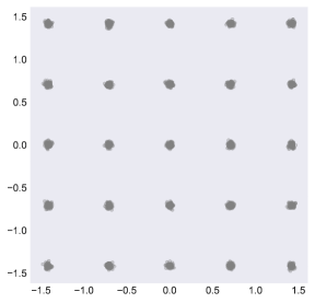
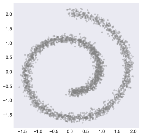
Figure 5: (Left) 25-Gaussian data (3,000 samples), and (Right) Swiss-roll data (3,000 samples).

D.2 Training

We used JAX (Bradbury et al., 2018) and Flax (Heek et al., 2023) to implement our score-based models with neural networks, and Optax (DeepMind et al., 2020) for the training.

As we write in the main part of this paper, we use simple neural network: $\mathbf{(}\mathbf{x},t)\to{\tt concat}([\mathbf{x},t])\to\big{(}{\tt Dense}(128)\to{\tt swish}\big{)}^{3}\to{\tt Dense}(2)\to{\bm{s}}_{\theta}(\mathbf{x},t)$ with default initialization both in training with Swiss-roll data and 25-Gaussian data. The loss function is calculated by Monte-Carlo sampling in each training step:

1. First we divide the time interval $[T_{\text{min}},T_{\text{max}}]$ into 1,000 equal parts in advance to get a discretized diffusion time array.

2. We take $N_{\text{batch}}=$ 512 batches of data $\{\mathbf{x}_{i}\}_{i=1,2,\dots,N_{\text{batch}}}$ and for each data point we take a discretized diffusion time $t_{i}$ uniformly from the array that we discretized in the first step.

3. We compute the signal $\alpha(t_{i})$ and noise $\sigma(t_{i})$ at time $t_{i}$, computed from the definition of SDE, and take the following quantities as approximations of the loss function

   $$\frac{1}{N_{\text{batch}}}\sum_{i=1}^{N_{\text{batch}}}\frac{g(t_{i})^{2}}{2}\left\|\frac{\mathbf{x}_{i,t}-\alpha(t_{i})\mathbf{x}_{i}}{\sigma(t_{i})^{2}}+{\bm{s}}_{\theta}(\mathbf{x}_{i,t},t_{i})\right\|^{2},$$ (108)

   where $\mathbf{x}_{i,t}\sim\mathcal{N}(\alpha(t_{i})\mathbf{x}_{i},\sigma(t_{i})^{2}I)$ is the Monte-Carlo sample.

The signal and noise functions $\alpha(t)$ and $\sigma(t)$ are:

$$\begin{split}&\text{\sc simple: }\quad\alpha(t)=e^{-\frac{\beta}{4}t^{2}},\quad\sigma(t)^{2}={1-e^{-\frac{\beta}{2}t^{2}}},\\ &\text{\sc cosine: }\quad\alpha(t)=\cos\left(\frac{\pi}{2}t\right),\quad\sigma(t)^{2}={1-\cos\left(\frac{\pi}{2}t\right)}.\end{split}$$ (109)

These expressions are derived from general argument of SDE. In general, once the SDE

$$d\mathbf{x}_{t}=f(t)\mathbf{x}+g(t)d\mathbf{w}_{t}$$ (110)

is given, the conditional probability from time $t=0$ to $t$ is given by

$$p_{t|0}(\mathbf{x}_{t}|\mathbf{x}_{0})=\mathcal{N}(\mathbf{x}_{t}|\alpha(t)\mathbf{x}_{0},\sigma(t)^{2}I),$$ (111)

where

$$\alpha(t)=e^{\int_{0}^{t}f(\xi){\rm d}\xi},\quad\sigma(t)^{2}=\alpha(t)^{2}\int_{0}^{t}\frac{g(\xi)^{2}}{\alpha(\xi)^{2}}{\rm d}\xi,$$ (112)

which is essentially equivalent to the formula in (Karras et al., 2022).

In training, 3,000 data points are taken in advance, and stochastic gradients are computed based on the Monte-Carlo loss function (108) with batch size 512 mini-batches. The gradients are used for optimization of the neural network ${\bm{s}}_{\theta}(\mathbf{x}_{t},t)$ with Adam-optimizer with learning rate 1e-3 and default values determined by Optax (DeepMind et al., 2020). We train our models 16,000 epochs.

D.3 Inference

Here we show some instances on generated data by our pretrained model in Figs. 9, 9, 9 and 9. The figures are plotted with identical points in discretized time, $t=1,\ 0.18,\ 0.1,\ 0.01$.

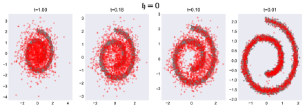
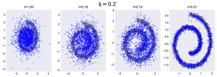
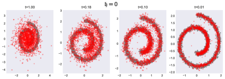
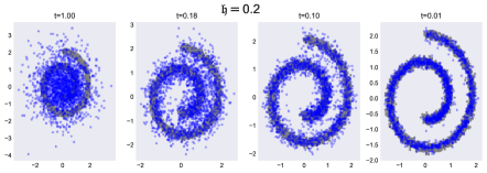
Figure 6: simple-sde pretrained model on Swiss-roll data with (Left) probability flow ODE ($\mathfrak{h}=0$), (Right) SDE (9) with $\mathfrak{h}=0.2$.

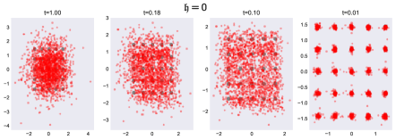
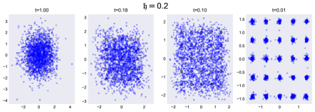
Figure 7: cosine-sde pretrained model on Swiss-roll data with (Left) probability flow ODE ($\mathfrak{h}=0$), (Right) SDE (9) with $\mathfrak{h}=0.2$.

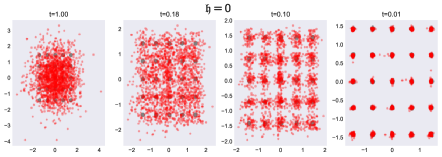
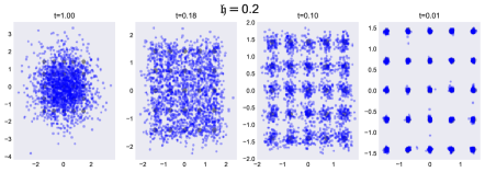
Figure 8: simple-sde pretrained model on 25-Gaussian data with (Left) probability flow ODE ($\mathfrak{h}=0$), (Right) SDE (9) with $\mathfrak{h}=0.2$.

Figure 9: cosine-sde pretrained model on 25-Gaussian data with (Left) probability flow ODE ($\mathfrak{h}=0$), (Right) SDE (9) with $\mathfrak{h}=0.2$.

Appendix E Derivative numerical error estimations in Sec. 5.2

E.1 Estimation of the local errors (23)

For simplicity, we omit “$\mathfrak{h}=0$” script here. In this notation, error of $\log q_{t}(\mathbf{x})$ and local errors (23) are

$$\begin{split}\text{err}(N[\log q_{t}(\mathbf{x})])&=\log q_{t}(\mathbf{x})-N[\log q_{t}(\mathbf{x})],\\ \text{err}(\hat{\nabla}N[\log q_{t}(\mathbf{x})])&=\nabla\log q_{t}(\mathbf{x})-\hat{\nabla}N[\log q_{t}(\mathbf{x})],\\ \text{err}(\hat{\nabla}^{2}N[\log q_{t}(\mathbf{x})])&=\nabla^{2}\log q_{t}(\mathbf{x})-\hat{\nabla}^{2}N[\log q_{t}(\mathbf{x})].\end{split}$$ (113)

We use a third-party solver scipy.integrate.solve_ivp (Virtanen et al., 2020), and it has inputs atol and rtol that control the errors in the subroutine, to make it clear, let us call the numerical value as $N_{{\tt atol},{\tt rtol}}[...]$. It is plausible to expect the order of errors are same between numerical calculations based on the same order of tolerances, say

$$\begin{split}O\Big{(}\text{err}(\hat{\nabla}^{0\text{ or }1\text{ or }2}N_{({\tt 1.1*atol}),({\tt 1.1*rtol})}[\log q_{t}(\mathbf{x})])\Big{)}=O\Big{(}\text{err}(\hat{\nabla}^{0\text{ or }1\text{ or }2}N_{{\tt atol},{\tt rtol}}[\log q_{t}(\mathbf{x})])\Big{)},\end{split}$$ (114)

where $O$ means order estimate. Based on this observation, we can estimate each error. For example,

$$\begin{split}&\underbrace{N_{({\tt 1.1*atol}),({\tt 1.1*rtol})}[\log q_{t}(\mathbf{x})]}_{\log q_{t}(\mathbf{x})+\text{err}(N_{({\tt 1.1*atol}),({\tt 1.1*rtol})}[\log q_{t}(\mathbf{x})])}-\underbrace{N_{{\tt atol},{\tt rtol}}[\log q_{t}(\mathbf{x})]}_{\log q_{t}(\mathbf{x})+\text{err}(N_{{\tt atol},{\tt rtol}}[\log q_{t}(\mathbf{x})])}\\ &=\text{err}(N_{({\tt 1.1*atol}),({\tt 1.1*rtol})}[\log q_{t}(\mathbf{x})])-\text{err}(N_{{\tt atol},{\tt rtol}}[\log q_{t}(\mathbf{x})])\\ &=O\Bigl{(}\text{err}(N_{{\tt atol},{\tt rtol}}[\log q_{t}(\mathbf{x})])\Bigr{)}.\end{split}$$ (115)

E.2 subtraction: Estimation of the local errors (23) by subtraction

On the order estimations for differential operators, we have 2 choices. First choice is estimating them simply by

$$\text{err}(\hat{\nabla}^{1\text{ or }2}N[\log q_{t}(\mathbf{x})])=\hat{\nabla}^{1\text{ or }2}N_{({\tt 1.1*atol}),({\tt 1.1*rtol})}[\log q_{t}(\mathbf{x})]-\hat{\nabla}^{1\text{ or }2}N_{{\tt atol},{\tt rtol}}[\log q_{t}(\mathbf{x})]$$ (116)

We name error estimation scheme based on this by subtraction. this method is straightforward, however, we need doubled computation time, and we introduce more time-efficient estimation in the next section.

E.3 model: Estimation of the local errors (23) by Taylor expansion and score models

Next choice is simply based on the error

$$N[\log q_{t}(\mathbf{x})]=\log q_{t}(\mathbf{x})+\text{err}(N[\log q_{t}(\mathbf{x})]).$$ (117)

By applying the discrete differential (21), we can get

$$\begin{split}\hat{\nabla}N[\log q_{t}(\mathbf{x})]&=\left[\begin{array}[]{l}\frac{N[\log q_{t}(\mathbf{x}_{t}+[\Delta x,0]^{\top})]-N[\log q_{t}(\mathbf{x}_{t}-[\Delta x,0]^{\top})]}{2\Delta x}\\ \frac{N[\log q_{t}(\mathbf{x}_{t}+[0,\Delta x]^{\top})]-N[\log q_{t}(\mathbf{x}_{t}-[0,\Delta x]^{\top})]}{2\Delta x}\end{array}\right].\end{split}$$ (118)

It would be sufficient to show $x$ component:

$$\begin{split}&\hat{\partial}_{x}N[\log q_{t}(\mathbf{x})]\\ &=\frac{N[\log q_{t}(\mathbf{x}+[\Delta x,0]^{\top})]-N[\log q_{t}(\mathbf{x}-[\Delta x,0]^{\top})]}{2\Delta x}\\ &=\frac{\log q_{t}(\mathbf{x}+[\Delta x,0]^{\top})-\log q_{t}(\mathbf{x}-[\Delta x,0]^{\top})}{2\Delta x}+\frac{\text{err}(N[\log q_{t}(\mathbf{x}+[\Delta x,0]^{\top})])-\text{err}(N[\log q_{t}(\mathbf{x}-[\Delta x,0]^{\top})])}{2\Delta x}\\ &=\frac{\partial_{x}\log q_{t}(\mathbf{x})2\Delta x+O(\Delta x^{3})}{2\Delta x}+\frac{O(\text{err}(N[\log q_{t}(\mathbf{x})]))}{\Delta x}\\ &=\partial_{x}\log q_{t}(\mathbf{x})+O(\Delta x^{2})+\frac{O(\text{err}(N[\log q_{t}(\mathbf{x})]))}{\Delta x},\end{split}$$ (119)

where we use the facts: 1) $O(\Delta x^{2})$ term vanishes from the numerator thanks to the symmetric descrete differential, 2) orders of $\text{err}(N[\log q_{t}(\mathbf{x}))]$ and $\text{err}(N[\log q_{t}(\mathbf{x}\pm[\Delta x,0]^{\top})])$ are same, in the 3rd line. This fact is achieved by the Runge-Kutta integrator. Therefore, by subtracting the true value from both side, we get

$$\text{err}(\hat{\nabla}N[\log q_{t}(\mathbf{x})])=\nabla\log q_{t}(\mathbf{x})-\hat{\nabla}N[\log q_{t}(\mathbf{x})]=O(\Delta x^{2})+\frac{O(\text{err}(N[\log q_{t}(\mathbf{x})]))}{\Delta x}$$ (120)

We can derive the error for $\nabla^{2}$ similarly:

$$\small\begin{split}&\hat{\nabla}^{2}N[\log q_{t}(\mathbf{x})]\\ &=\frac{N[\log q_{t}(\mathbf{x}+[\Delta x,0]^{\top})]+N[\log q_{t}(\mathbf{x}-[\Delta x,0]^{\top})]+N[\log q_{t}(\mathbf{x}+[0,\Delta x]^{\top})]+N[\log q_{t}(\mathbf{x}-[0,\Delta x]^{\top})]-4N[\log q_{t}(\mathbf{x})]}{\Delta x^{2}}\\ &=\frac{\log q_{t}(\mathbf{x}+[\Delta x,0]^{\top})+\log q_{t}(\mathbf{x}-[\Delta x,0]^{\top})+\log q_{t}(\mathbf{x}+[0,\Delta x]^{\top})+\log q_{t}(\mathbf{x}-[0,\Delta x]^{\top})-4\log q_{t}(\mathbf{x})}{\Delta x^{2}}\\ &\quad+\frac{\begin{array}[]{r}\text{err}(N[\log q_{t}(\mathbf{x}+[\Delta x,0]^{\top})])+\text{err}(N[\log q_{t}(\mathbf{x}-[\Delta x,0]^{\top})])+\text{err}(N[\log q_{t}(\mathbf{x}+[0,\Delta x]^{\top})])+\text{err}(N[\log q_{t}(\mathbf{x}-[0,\Delta x]^{\top})])\\ -4\text{err}(N[\log q_{t}(\mathbf{x})])\end{array}}{\Delta x^{2}}\\ &=\frac{\nabla^{2}\log q_{t}(\mathbf{x})\Delta x^{2}+O(\Delta x^{4})}{\Delta x^{2}}+\frac{O(\text{err}(N[\log q_{t}(\mathbf{x})]))}{\Delta x^{2}}\\ &=\nabla^{2}\log q_{t}(\mathbf{x})+O(\Delta x^{2})+\frac{O(\text{err}(N[\log q_{t}(\mathbf{x})]))}{\Delta x^{2}},\end{split}\normalsize$$ (121)

where we use that $O(\Delta x^{3})$ term in the numerator vanishes because we use the 5-point approximation of the laplacian. Now we get

$$\text{err}(\hat{\nabla}^{2}N[\log q_{t}(\mathbf{x})])=\nabla^{2}\log q_{t}(\mathbf{x})-\hat{\nabla}^{2}N[\log q_{t}(\mathbf{x})]=O(\Delta x^{2})+\frac{O(\text{err}(N[\log q_{t}(\mathbf{x})]))}{\Delta x^{2}}$$ (122)

In summary, we conclude each error as

$$\begin{split}\text{err}(\hat{\nabla}N[\log q_{t}(\mathbf{x})])&={\bm{C}}^{(1)}_{t}(\mathbf{x})\Delta x^{2}+\frac{O(\text{err}(N[\log q_{t}(\mathbf{x})]))\mathbf{1}}{\Delta x},\\ \text{err}(\hat{\nabla}^{2}N[\log q_{t}(\mathbf{x})])&=C^{(2)}_{t}(\mathbf{x})\Delta x^{2}+\frac{O(\text{err}(N[\log q_{t}(\mathbf{x})]))}{\Delta x^{2}},\end{split}$$ (123)

where $\mathbf{1}$ is the vector with all 1 components, and ${\bm{C}}^{(1)}_{t}(\mathbf{x}),C^{(2)}_{t}(\mathbf{x})$ are determined by the Taylor expansion remainder terms. Typically, these are approximated by

$$\begin{split}{\bm{C}}^{(1)}_{t}(\mathbf{x})&\approx\text{3rd derivative of }\log q_{t}(\mathbf{x}),\\ C^{(2)}_{t}(\mathbf{x})&\approx\text{4th derivative of }\log q_{t}(\mathbf{x}).\end{split}$$ (124)

Of course, we cannot access to the functions (124), however, it would be plausible to regard

$$O(\nabla\log q_{t}(\mathbf{x}))=O(\bm{s}_{\theta}(\mathbf{x},t)),$$ (125)

because the objective of the diffusion model training is to achieve $\bm{s}_{\theta}(\mathbf{x},t)\approx\nabla\log p_{t}(\mathbf{x})$ and in the ideal case, $q_{t}=p_{t}$. By using this assumption, we regard

$$\begin{split}{\bm{C}}^{(1)}_{t}(\mathbf{x})&\approx-\nabla(\nabla\cdot\bm{s}_{\theta}(\mathbf{x},t))\\ C^{(2)}_{t}(\mathbf{x})&\approx-\nabla^{2}(\nabla\cdot\bm{s}_{\theta}(\mathbf{x},t))\end{split}$$ (126)

and estimate the local errors by

$$\begin{split}\text{err}(\hat{\nabla}N[\log q_{t}(\mathbf{x})])&\approx|\nabla(\nabla\cdot\bm{s}_{\theta}(\mathbf{x},t))\Delta x^{2}|+\left|\frac{O(\text{err}(N[\log q_{t}(\mathbf{x})]))\mathbf{1}}{\Delta x}\right|,\\ \text{err}(\hat{\nabla}^{2}N[\log q_{t}(\mathbf{x})])&\approx|\nabla^{2}(\nabla\cdot\bm{s}_{\theta}(\mathbf{x},t))\Delta x^{2}|+\left|\frac{O(\text{err}(N[\log q_{t}(\mathbf{x})]))}{\Delta x^{2}}\right|,\end{split}$$ (127)

where $O(\text{err}(N[\log q_{t}(\mathbf{x})]))$ can be estimated by using (115). We name error estimation scheme based on this by model.

E.4 Integral of the local errors

Now we go back to Theorem 4.2 to explain our error estimation for $O(\mathfrak{h})$ correction to the (negative) log-likelihood. To calculate $O(\mathfrak{h})$ terms, we consider the paired ODE constructed by

$$\begin{split}\dot{\mathbf{x}}_{t}&=\bm{f}^{\rm PF}_{\theta}(\mathbf{x}_{t},t),\\ \dot{\delta\mathbf{x}}_{t}&=\delta{\bm{f}}^{\rm PF}_{\theta}(\mathbf{x}_{t},\delta\mathbf{x}_{t},t)\quad(\text{by }\hat{\nabla}N[\log q_{t}(\mathbf{x}_{t})]),\\ \dot{\delta\log q_{t}}&=\nabla\cdot\delta{\bm{f}}^{\rm PF}_{\theta}(\mathbf{x}_{t},\delta\mathbf{x}_{t},t)\quad(\text{by }\hat{\nabla}^{2}N[\log q_{t}(\mathbf{x}_{t})]),\end{split}$$ (128)

as we wrote in Algorithm 1. In this expression, there is no numerical error in the RHS of $\dot{\mathbf{x}}_{t}$ except for the float32 precision that is the default of the deep learning framework. In the RHS of $\dot{\delta\mathbf{x}}_{t}$, we have discretization of differential $\hat{\nabla}$ and numerical integral for $\log q^{\mathfrak{h}=0}_{t}(\mathbf{x}_{t})$, and as we noted, we omit $\mathfrak{h}=0$ and call it as $\log q_{t}(\mathbf{x}_{t})$. By using the error estimation (127), we rewrite ODE for ${\delta\mathbf{x}}_{t}$ as

$$\begin{split}\dot{\delta\mathbf{x}}_{t}&=(\delta\mathbf{x}_{t}\cdot\nabla)\bm{f}^{\rm PF}_{\theta}(\mathbf{x}_{t},t)-\frac{g(t)^{2}}{2}(\bm{s}_{\theta}(\mathbf{x}_{t},t)-\underbrace{\hat{\nabla}N\log q_{t}(\mathbf{x}_{t})}_{{\nabla}\log q_{t}(\mathbf{x}_{t})+\text{err}(\hat{\nabla}N[\log q_{t}(\mathbf{x}_{t})])})\\ &=(\delta\mathbf{x}_{t}\cdot\nabla)\bm{f}^{\rm PF}_{\theta}(\mathbf{x}_{t},t)-\frac{g(t)^{2}}{2}(\bm{s}_{\theta}(\mathbf{x}_{t},t)-{\nabla}\log q_{t}(\mathbf{x}_{t}))+\frac{g(t)^{2}}{2}\text{err}(\hat{\nabla}N[\log q_{t}(\mathbf{x}_{t})]).\end{split}$$ (129)

When we apply the solver, basically it discretize the system as

$$\begin{split}\delta\mathbf{x}_{t+\epsilon}=\delta\mathbf{x}_{t}+\epsilon\Big{(}(\delta\mathbf{x}_{t}\cdot\nabla)\bm{f}^{\rm PF}_{\theta}(\mathbf{x}_{t},t)-\frac{g(t)^{2}}{2}(\bm{s}_{\theta}(\mathbf{x}_{t},t)-{\nabla}\log q_{t}(\mathbf{x}_{t}))+\frac{g(t)^{2}}{2}\text{err}(\hat{\nabla}N[\log q_{t}(\mathbf{x}_{t})])\Big{)}+\dots,\end{split}$$ (130)

and truncate $\dots$ terms up to certain finite order, and apply this recursive equation from $\delta\mathbf{x}_{0}$. For simplicity, we consider the liner term only here, and split $\delta\mathbf{x}_{t}=\delta\mathbf{x}_{t}^{\text{true}}+\text{err}^{(1)}_{t}$, then

$$\begin{split}&\begin{pmatrix}\delta\mathbf{x}_{t+\epsilon}^{\text{true}}\\ +\\ \text{err}^{(1)}_{t+\epsilon}\end{pmatrix}\\ &=\begin{pmatrix}\delta\mathbf{x}_{t}^{\text{true}}\\ +\\ \text{err}^{(1)}_{t}\end{pmatrix}+\epsilon\Big{(}\left(\begin{pmatrix}\delta\mathbf{x}_{t}^{\text{true}}\\ +\\ \text{err}^{(1)}_{t}\end{pmatrix}\cdot\nabla\right)\bm{f}^{\rm PF}_{\theta}(\mathbf{x}_{t},t)-\frac{g(t)^{2}}{2}(\bm{s}_{\theta}(\mathbf{x}_{t},t)-{\nabla}\log q_{t}(\mathbf{x}_{t}))+\frac{g(t)^{2}}{2}\text{err}(\hat{\nabla}N[\log q_{t}(\mathbf{x}_{t})])\Big{)}\\ &=\begin{pmatrix}\delta\mathbf{x}_{t}^{\text{true}}+\epsilon\Big{(}(\delta\mathbf{x}_{t}^{\text{true}}\cdot\nabla)\bm{f}^{\rm PF}_{\theta}(\mathbf{x}_{t},t)-\frac{g(t)^{2}}{2}(\bm{s}_{\theta}(\mathbf{x}_{t},t)-{\nabla}\log q_{t}(\mathbf{x}_{t}))\Big{)}\\ +\\ \text{err}^{(1)}_{t}+\epsilon\Big{(}(\text{err}^{(1)}_{t}\cdot\nabla)\bm{f}^{\rm PF}_{\theta}(\mathbf{x}_{t},t)+\frac{g(t)^{2}}{2}\text{err}(\hat{\nabla}N[\log q_{t}(\mathbf{x}_{t})])\Big{)}\end{pmatrix},\end{split}$$ (131)

and we get the ODE for time $t$ error by taking continuous time limit:

$$\dot{\text{err}}^{(1)}_{t}=(\text{err}^{(1)}_{t}\cdot\nabla)\bm{f}^{\rm PF}_{\theta}(\mathbf{x}_{t},t)+\frac{g(t)^{2}}{2}\text{err}(\hat{\nabla}N[\log q_{t}(\mathbf{x}_{t})]).$$ (132)

Note that $\text{err}^{(1)}_{t}$ is a vector with same dimension to $\mathbf{x}_{t},\delta\mathbf{x}_{t},\bm{s}_{\theta}$, and $\bm{f}^{\rm PF}_{\theta}$. As same, we can get the ODE for $\dot{\delta\log q_{t}}$ term. The discrete ODE is

$$\begin{split}&\delta\log q_{t+\epsilon}\\ &=\delta\log q_{t}+\epsilon\Big{(}(\delta\mathbf{x}_{t}\cdot\nabla)\nabla\cdot\bm{f}^{\rm PF}_{\theta}(\mathbf{x}_{t},t)-\frac{g(t)^{2}}{2}(\nabla\cdot\bm{s}_{\theta}(\mathbf{x}_{t},t)-{\nabla}^{2}\log q_{t}(\mathbf{x}_{t}))+\frac{g(t)^{2}}{2}\text{err}(\hat{\nabla}^{2}N[\log q_{t}(\mathbf{x}_{t})])\Big{)}+\dots,\end{split}$$ (133)

and as same, by splitting true value and error value, we get

$$\begin{split}&\begin{pmatrix}\delta\log q_{t+\epsilon}^{\text{true}}\\ +\\ \text{err}^{(2)}_{t+\epsilon}\end{pmatrix}\\ &=\begin{pmatrix}\delta\log q_{t}^{\text{true}}+\epsilon\Big{(}(\delta\mathbf{x}_{t}^{\text{true}}\cdot\nabla)\nabla\cdot\bm{f}^{\rm PF}_{\theta}(\mathbf{x}_{t},t)-\frac{g(t)^{2}}{2}(\nabla\cdot\bm{s}_{\theta}(\mathbf{x}_{t},t)-{\nabla}^{2}\log q_{t}(\mathbf{x}_{t}))\Big{)}\\ +\\ \text{err}^{(2)}_{t}+\epsilon\Bigl{(}(\text{err}^{(1)}_{t}\cdot\nabla)\nabla\cdot\bm{f}^{\rm PF}_{\theta}(\mathbf{x}_{t},t)+\frac{g(t)^{2}}{2}\text{err}(\hat{\nabla}^{2}N[\log q_{t}(\mathbf{x}_{t})])\Bigr{)}\end{pmatrix},\end{split}$$ (134)

and get the ODE for $\text{err}^{(2)}_{t}$ as

$$\dot{\text{err}}^{(2)}_{t}=(\text{err}^{(1)}_{t}\cdot\nabla)\nabla\cdot\bm{f}^{\rm PF}_{\theta}(\mathbf{x}_{t},t)+\frac{g(t)^{2}}{2}\text{err}(\hat{\nabla}^{2}N[\log q_{t}(\mathbf{x}_{t})]).$$ (135)

In summary, we get the ODE system

$$\begin{split}\dot{\mathbf{x}}_{t}&=\bm{f}^{\rm PF}_{\theta}(\mathbf{x}_{t},t),\\ \dot{\delta\mathbf{x}}_{t}&=\delta{\bm{f}}^{\rm PF}_{\theta}(\mathbf{x}_{t},\delta\mathbf{x}_{t},t)\quad(\text{by }\hat{\nabla}N[\log q_{t}(\mathbf{x}_{t})]),\\ \dot{\delta\log q_{t}}&=\nabla\cdot\delta{\bm{f}}^{\rm PF}_{\theta}(\mathbf{x}_{t},\delta\mathbf{x}_{t},t)\quad(\text{by }\hat{\nabla}^{2}N[\log q_{t}(\mathbf{x}_{t})]),\\ \dot{\text{err}}^{(1)}_{t}&=(\text{err}^{(1)}_{t}\cdot\nabla)\bm{f}^{\rm PF}_{\theta}(\mathbf{x}_{t},t)+\frac{g(t)^{2}}{2}\text{err}(\hat{\nabla}N[\log q_{t}(\mathbf{x}_{t})]),\\ \dot{\text{err}}^{(2)}_{t}&=(\text{err}^{(1)}_{t}\cdot\nabla)\nabla\cdot\bm{f}^{\rm PF}_{\theta}(\mathbf{x}_{t},t)+\frac{g(t)^{2}}{2}\text{err}(\hat{\nabla}^{2}N[\log q_{t}(\mathbf{x}_{t})]).\end{split}$$ (136)

The errors in Table 1 are calculated by solving more conservative (or over-estimated) ODE:

$$\begin{split}\dot{\text{err}}^{(1)}_{t}&=\Big{|}(\text{err}^{(1)}_{t}\cdot\nabla)\bm{f}^{\rm PF}_{\theta}(\mathbf{x}_{t},t)\Big{|}+\Big{|}\frac{g(t)^{2}}{2}\text{err}(\hat{\nabla}N[\log q_{t}(\mathbf{x}_{t})])\Big{|},\\ \dot{\text{err}}^{(2)}_{t}&=\Big{|}(\text{err}^{(1)}_{t}\cdot\nabla)\nabla\cdot\bm{f}^{\rm PF}_{\theta}(\mathbf{x}_{t},t)\Big{|}+\Big{|}\frac{g(t)^{2}}{2}\text{err}(\hat{\nabla}^{2}N[\log q_{t}(\mathbf{x}_{t})])\Big{|},\end{split}$$ (137)

by using approximations (127) and the error final value for $\log q_{T}$ as

$$|\text{err}^{(1)}_{T}\cdot\nabla\log\pi(\mathbf{x}_{T})|+|\text{err}^{(2)}_{T}|$$ (138)

E.5 Visualization of local error estimates

Of course, the degree of final error (138) strongly depends on the order of the local errors $\text{err}(\hat{\nabla}N[\log q_{t}(\mathbf{x}_{t})])$ and $\text{err}(\hat{\nabla}^{2}N[\log q_{t}(\mathbf{x}_{t})])$. To see its order, we plot $\log_{10}$ scales of the local error functions in Fig. 14.

If we believe $\text{err}(N[\log q_{t}(\mathbf{x})])$ is suppressed within the small tolerance value, we take it as $10^{-5}$ by the Runge-Kutta algorithm, the order of local errors are depending on the coefficients of $\Delta x^{2}$. To check these values, we plot mean and std values of $\text{tr}\nabla(\nabla\cdot{\bm{s}}_{\theta}(\mathbf{x},t))$ and $\nabla^{2}(\nabla\cdot{\bm{s}}_{\theta}(\mathbf{x},t))$ by sampling 500 points $\mathbf{x}\sim\text{Uniform}(\min({\tt validation\ set})-0.1,\max({\tt validation\ set})-0.1)$ at each time $t$ in Figs. 14, 14, 14 and 14. Simultaneously, we plot colored contours that corresponds the value of local error estimates based on (126) with $\Delta x=0.01$, that are exactly same as the values on dashed line in Fig. 14.

From these figures, one can see that the estimated local errors are almost located at safe region, i.e., errors are negative in log scale. As one can see, the 25-Gaussian case Figs. 14 and 14, the maximum values are slightly inside red regions, and we may be careful about it, but we leave further study as a future work.

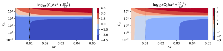
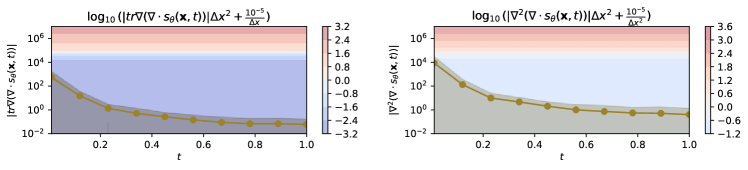
Figure 10: The order of local errors. (Left) Contour plot corresponding to $\text{err}(\hat{\nabla}N[\log q_{t}(\mathbf{x}_{t})])$. (Right) Contour plot corresponding to $\text{err}(\hat{\nabla}^{2}N[\log q_{t}(\mathbf{x}_{t})])$, based on (126). Blue region has negative power, and relatively safe. Red region has positive power, and dangerous. The dotted line corresponds $\Delta x=0.01$ that is the value used in Table 1. The value $10^{-5}$ in the 2nd-term numerator is the typical tolerance value of 0th-logqSolver in Algorithm 1, that corresponds to $\text{err}(N[\log q_{t}(\mathbf{x})])$.

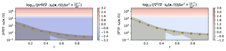
Figure 11: Local error mean/std plot with pretrained model with simple-SDE trained by Swiss-roll.

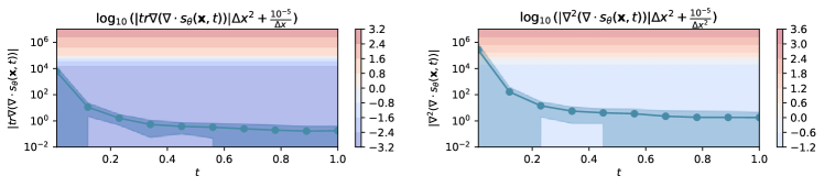
Figure 12: Local error mean/std plot with pretrained model with cosine-SDE trained by Swiss-roll.

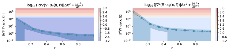
Figure 13: Local error mean/std plot with pretrained model with simple-SDE trained by 25-Gaussian.

Figure 14: Local error mean/std plot with pretrained model with cosine-SDE trained by 25-Gaussian.

References

• Anderson (1982) Anderson, B. D. Reverse-time diffusion equation models. Stochastic Processes and their Applications, 12(3):313–326, 1982.
• Bradbury et al. (2018) Bradbury, J., Frostig, R., Hawkins, P., Johnson, M. J., Leary, C., Maclaurin, D., Necula, G., Paszke, A., VanderPlas, J., Wanderman-Milne, S., and Zhang, Q. JAX: composable transformations of Python+NumPy programs, 2018. URL http://github.com/google/jax.
• Chen et al. (2018) Chen, R. T., Rubanova, Y., Bettencourt, J., and Duvenaud, D. K. Neural ordinary differential equations. Advances in neural information processing systems, 31, 2018.
• Damgaard & Hüffel (1987) Damgaard, P. H. and Hüffel, H. Stochastic quantization. Physics Reports, 152(5):227–398, 1987. ISSN 0370-1573. doi: https://doi.org/10.1016/0370-1573(87)90144-X. URL https://www.sciencedirect.com/science/article/pii/037015738790144X.
• De Bortoli et al. (2021) De Bortoli, V., Thornton, J., Heng, J., and Doucet, A. Diffusion schrödinger bridge with applications to score-based generative modeling. In Ranzato, M., Beygelzimer, A., Dauphin, Y., Liang, P., and Vaughan, J. W. (eds.), Advances in Neural Information Processing Systems, volume 34, pp.  17695–17709. Curran Associates, Inc., 2021. URL https://proceedings.neurips.cc/paper_files/paper/2021/file/940392f5f32a7ade1cc201767cf83e31-Paper.pdf.
• DeepMind et al. (2020) DeepMind, Babuschkin, I., Baumli, K., Bell, A., Bhupatiraju, S., Bruce, J., Buchlovsky, P., Budden, D., Cai, T., Clark, A., Danihelka, I., Dedieu, A., Fantacci, C., Godwin, J., Jones, C., Hemsley, R., Hennigan, T., Hessel, M., Hou, S., Kapturowski, S., Keck, T., Kemaev, I., King, M., Kunesch, M., Martens, L., Merzic, H., Mikulik, V., Norman, T., Papamakarios, G., Quan, J., Ring, R., Ruiz, F., Sanchez, A., Sartran, L., Schneider, R., Sezener, E., Spencer, S., Srinivasan, S., Stanojević, M., Stokowiec, W., Wang, L., Zhou, G., and Viola, F. The DeepMind JAX Ecosystem, 2020. URL http://github.com/google-deepmind.
• Dhariwal & Nichol (2021) Dhariwal, P. and Nichol, A. Diffusion models beat gans on image synthesis. Advances in neural information processing systems, 34:8780–8794, 2021.
• Feynman (1948) Feynman, R. P. Space-time approach to non-relativistic quantum mechanics. Rev. Mod. Phys., 20:367–387, Apr 1948. doi: 10.1103/RevModPhys.20.367. URL https://link.aps.org/doi/10.1103/RevModPhys.20.367.
• Feynman & Hibbs (1965) Feynman, R. P. and Hibbs, A. R. Quantum mechanics and path integrals. International series in pure and applied physics. McGraw-Hill, New York, NY, 1965.
• Flamary et al. (2021) Flamary, R., Courty, N., Gramfort, A., Alaya, M. Z., Boisbunon, A., Chambon, S., Chapel, L., Corenflos, A., Fatras, K., Fournier, N., Gautheron, L., Gayraud, N. T., Janati, H., Rakotomamonjy, A., Redko, I., Rolet, A., Schutz, A., Seguy, V., Sutherland, D. J., Tavenard, R., Tong, A., and Vayer, T. Pot: Python optimal transport. Journal of Machine Learning Research, 22(78):1–8, 2021. URL http://jmlr.org/papers/v22/20-451.html.
• Heek et al. (2023) Heek, J., Levskaya, A., Oliver, A., Ritter, M., Rondepierre, B., Steiner, A., and van Zee, M. Flax: A neural network library and ecosystem for JAX, 2023. URL http://github.com/google/flax.
• Heusel et al. (2017) Heusel, M., Ramsauer, H., Unterthiner, T., Nessler, B., and Hochreiter, S. Gans trained by a two time-scale update rule converge to a local nash equilibrium. Advances in neural information processing systems, 30, 2017.
• Ho et al. (2020) Ho, J., Jain, A., and Abbeel, P. Denoising diffusion probabilistic models. Advances in neural information processing systems, 33:6840–6851, 2020.
• Huang et al. (2021a) Huang, C.-W., Lim, J. H., and Courville, A. C. A variational perspective on diffusion-based generative models and score matching. In Ranzato, M., Beygelzimer, A., Dauphin, Y., Liang, P., and Vaughan, J. W. (eds.), Advances in Neural Information Processing Systems, volume 34, pp.  22863–22876. Curran Associates, Inc., 2021a. URL https://proceedings.neurips.cc/paper_files/paper/2021/file/c11abfd29e4d9b4d4b566b01114d8486-Paper.pdf.
• Huang et al. (2021b) Huang, C.-W., Lim, J. H., and Courville, A. C. A variational perspective on diffusion-based generative models and score matching. Advances in Neural Information Processing Systems, 34:22863–22876, 2021b.
• Hyvärinen et al. (2009) Hyvärinen, A., Hurri, J., Hoyer, P. O., Hyvärinen, A., Hurri, J., and Hoyer, P. O. Estimation of non-normalized statistical models. Natural Image Statistics: A Probabilistic Approach to Early Computational Vision, pp.  419–426, 2009.
• Karras et al. (2022) Karras, T., Aittala, M., Aila, T., and Laine, S. Elucidating the design space of diffusion-based generative models. Advances in Neural Information Processing Systems, 35:26565–26577, 2022.
• Kingma et al. (2021) Kingma, D., Salimans, T., Poole, B., and Ho, J. Variational diffusion models. Advances in neural information processing systems, 34:21696–21707, 2021.
• Kingma & Gao (2023) Kingma, D. P. and Gao, R. Understanding the diffusion objective as a weighted integral of elbos. arXiv preprint arXiv:2303.00848, 2023.
• Kong et al. (2023) Kong, X., Brekelmans, R., and Steeg, G. V. Information-theoretic diffusion. 11th International Conference on Learning Representations, 2023.
• Lai et al. (2023) Lai, C.-H., Takida, Y., Murata, N., Uesaka, T., Mitsufuji, Y., and Ermon, S. FP-diffusion: Improving score-based diffusion models by enforcing the underlying score fokker-planck equation. In Krause, A., Brunskill, E., Cho, K., Engelhardt, B., Sabato, S., and Scarlett, J. (eds.), Proceedings of the 40th International Conference on Machine Learning, volume 202 of Proceedings of Machine Learning Research, pp.  18365–18398. PMLR, 23–29 Jul 2023. URL https://proceedings.mlr.press/v202/lai23d.html.
• Lipman et al. (2023) Lipman, Y., Chen, R. T., Ben-Hamu, H., Nickel, M., and Le, M. Flow matching for generative modeling. 11th International Conference on Learning Representations, 2023.
• Lu et al. (2022) Lu, C., Zheng, K., Bao, F., Chen, J., Li, C., and Zhu, J. Maximum likelihood training for score-based diffusion ODEs by high order denoising score matching. In Chaudhuri, K., Jegelka, S., Song, L., Szepesvari, C., Niu, G., and Sabato, S. (eds.), Proceedings of the 39th International Conference on Machine Learning, volume 162 of Proceedings of Machine Learning Research, pp.  14429–14460. PMLR, 17–23 Jul 2022. URL https://proceedings.mlr.press/v162/lu22f.html.
• Machlup & Onsager (1953) Machlup, S. and Onsager, L. Fluctuations and irreversible process. ii. systems with kinetic energy. Phys. Rev., 91:1512–1515, Sep 1953. doi: 10.1103/PhysRev.91.1512. URL https://link.aps.org/doi/10.1103/PhysRev.91.1512.
• Messiah (1970) Messiah, A. Quantum Mechanics Volume I. North-Holland Publishing Company, 1970.
• Nelson (1966) Nelson, E. Derivation of the schrödinger equation from newtonian mechanics. Phys. Rev., 150:1079–1085, Oct 1966. doi: 10.1103/PhysRev.150.1079. URL https://link.aps.org/doi/10.1103/PhysRev.150.1079.
• Oksendal (2013) Oksendal, B. Stochastic differential equations: an introduction with applications. Springer Science & Business Media, 2013.
• Onsager & Machlup (1953) Onsager, L. and Machlup, S. Fluctuations and irreversible processes. Phys. Rev., 91:1505–1512, Sep 1953. doi: 10.1103/PhysRev.91.1505. URL https://link.aps.org/doi/10.1103/PhysRev.91.1505.
• Pedregosa et al. (2011) Pedregosa, F., Varoquaux, G., Gramfort, A., Michel, V., Thirion, B., Grisel, O., Blondel, M., Prettenhofer, P., Weiss, R., Dubourg, V., Vanderplas, J., Passos, A., Cournapeau, D., Brucher, M., Perrot, M., and Duchesnay, E. Scikit-learn: Machine learning in Python. Journal of Machine Learning Research, 12:2825–2830, 2011.
• Petzka et al. (2018) Petzka, H., Fischer, A., and Lukovnicov, D. On the regularization of wasserstein gans. 6th International Conference on Learning Representations, 2018.
• Premkumar (2023) Premkumar, A. Generative diffusion from an action principle. arXiv preprint arXiv:2310.04490, 2023.
• Rombach et al. (2022) Rombach, R., Blattmann, A., Lorenz, D., Esser, P., and Ommer, B. High-resolution image synthesis with latent diffusion models. In Proceedings of the IEEE/CVF conference on computer vision and pattern recognition, pp.  10684–10695, 2022.
• Sohl-Dickstein et al. (2015) Sohl-Dickstein, J., Weiss, E., Maheswaranathan, N., and Ganguli, S. Deep unsupervised learning using nonequilibrium thermodynamics. In International conference on machine learning, pp.  2256–2265. PMLR, 2015.
• Song & Ermon (2019) Song, Y. and Ermon, S. Generative modeling by estimating gradients of the data distribution. Advances in neural information processing systems, 32, 2019.
• Song et al. (2021a) Song, Y., Durkan, C., Murray, I., and Ermon, S. Maximum likelihood training of score-based diffusion models. Advances in Neural Information Processing Systems, 34:1415–1428, 2021a.
• Song et al. (2021b) Song, Y., Sohl-Dickstein, J., Kingma, D. P., Kumar, A., Ermon, S., and Poole, B. Score-based generative modeling through stochastic differential equations. 9th International Conference on Learning Representations, 2021b.
• Su et al. (2023) Su, X., Song, J., Meng, C., and Ermon, S. Dual diffusion implicit bridges for image-to-image translation. In The Eleventh International Conference on Learning Representations, 2023. URL https://openreview.net/forum?id=5HLoTvVGDe.
• Vincent (2011) Vincent, P. A connection between score matching and denoising autoencoders. Neural computation, 23(7):1661–1674, 2011.
• Virtanen et al. (2020) Virtanen, P., Gommers, R., Oliphant, T. E., Haberland, M., Reddy, T., Cournapeau, D., Burovski, E., Peterson, P., Weckesser, W., Bright, J., van der Walt, S. J., Brett, M., Wilson, J., Millman, K. J., Mayorov, N., Nelson, A. R. J., Jones, E., Kern, R., Larson, E., Carey, C. J., Polat, İ., Feng, Y., Moore, E. W., VanderPlas, J., Laxalde, D., Perktold, J., Cimrman, R., Henriksen, I., Quintero, E. A., Harris, C. R., Archibald, A. M., Ribeiro, A. H., Pedregosa, F., van Mulbregt, P., and SciPy 1.0 Contributors. SciPy 1.0: Fundamental Algorithms for Scientific Computing in Python. Nature Methods, 17:261–272, 2020. doi: 10.1038/s41592-019-0686-2.
• Wang et al. (2023) Wang, L., Aarts, G., and Zhou, K. Diffusion models as stochastic quantization in lattice field theory. arXiv preprint arXiv:2309.17082, 2023.
• Yang et al. (2023) Yang, L., Zhang, Z., Song, Y., Hong, S., Xu, R., Zhao, Y., Zhang, W., Cui, B., and Yang, M.-H. Diffusion models: A comprehensive survey of methods and applications. ACM Computing Surveys, 56(4):1–39, 2023.
• Zhang & Chen (2023) Zhang, Q. and Chen, Y. Fast sampling of diffusion models with exponential integrator. 11th International Conference on Learning Representations, 2023.