Speed, Accuracy, and Complexity

DDMonthYYYY  []

Speed, Accuracy, and Complexity

Duarte Gonçalves

Abstract

This paper re-examines the validity of using response time to infer problem complexity. It revisits a canonical Wald model of optimal stopping, taking signal-to-noise ratio as a measure of problem complexity. While choice quality is monotone in problem complexity, expected stopping time is inverse $U$-shaped. Indeed decisions are fast in both very simple and very complex problems: in simple problems it is quick to understand which alternative is best, while in complex problems it would be too costly — an insight which extends to general costly information acquisition models. This non-monotonicity also underlies an ambiguous relationship between response time and ability, whereby higher ability entails slower decisions in very complex problems, but faster decisions in simple problems. Finally, this paper proposes a new method to correctly infer problem complexity based on the finding that choices react more to changes in incentives in more complex problems.  

Keywords: Sequential Sampling; Complexity; Information Acquisition; Drift-Diffusion; Statistical Decision Theory.
JEL Classifications: D83, D84, D90.

1.  Introduction

It is almost definitional that more complex decision problems entail more mistakes. Individuals make more mistakes and choose dominated alternatives in more complex environments, both in experimental settings (e.g. Rabin and Weizsäcker, 2009; Martínez-Marquina et al., 2019; Banovetz and Oprea, 2023; Enke, 2020) and in real-world decisions with significant financial implications — e.g. selecting health insurance plans (Sinaiko and Hirth, 2011; Bhargava et al., 2017), pension plans (Choi et al., 2011), and mortgages (Keys et al., 2016; Agarwal et al., 2016). This has important implications, since deploying theoretically optimal but complex incentive structures (tax schedules, allocation mechanisms, pricing schemes, etc) may lead to unreliable predictions and suboptimal outcomes — an observation at the root of the ongoing focus on simple mechanisms, both in theoretical (Li, 2017; Börgers and Li, 2019; Pycia and Troyan, 2023) and in empirical work (Rees-Jones and Taubinsky, 2020). If problem complexity is taken to be a leading explanation of suboptimal decision-making, understanding which problems are more complex becomes crucial for simplifying them.

Response time is often used as an indicator of problem complexity in various settings, including lottery choice (Wilcox, 1993), loans (Kalaycı and Serra-Garcia, 2016), and portfolio selection (Carvalho and Silverman, 2017). Going beyond economics, a large literature in psychology and neuroscience has also used response time as a proxy for problem complexity (Ratcliff and McKoon, 2008; Shadlen and Shohamy, 2016; Bogacz et al., 2010). The underlying assumption is that in more complex problems, making similarly good choices requires greater cognitive effort, and response time can serve as a proxy for cognitive effort (Caplin et al., 2020). If decision-makers are able to make more accurate choices while expending less cognitive effort, as indicated by faster responses, then the decision problem is considered simpler. Therefore, a decision problem is deemed simpler if individuals make fewer mistakes (more accurate choices) and do so with less cognitive effort (faster choices).

The reliance on response time as a proxy for problem complexity is based on the observation that, in many cases, faster choices tend to be more accurate. For example, research in cognitive sciences has indicated that perceptual problems that are harder to discern require greater cognitive effort, leading to slower and less accurate decisions (e.g. Forstmann et al., 2016). Additionally, studies have found that decision-makers take longer when they are closest to being indifferent, indicating the difficulty in distinguishing the best alternative (Mosteller and Nogee, 1951; Krajbich et al., 2012; Clithero, 2018; Alós-Ferrer and Garagnani, 2022). This intuition aligns with sequential sampling models (Fudenberg et al., 2018; Gonçalves, 2023; Alós-Ferrer et al., 2021), where decisions take longer when individuals are closer to being indifferent, as the value of information is highest in such cases. In short, the justification behind the use of response times as a proxy for problem complexity is straightforward: a problem is considered easier if choices are both faster and more accurate, with faster choices often implying greater accuracy.

Whilst response time may be a compelling indicator of problem complexity, it may not always be a reliable measure when used on its own. The existing literature documents a more ambiguous relationship between speed and accuracy, where in some cases faster decisions are better whereas in others slower decisions are more accurate (e.g. Achtziger and Alós-Ferrer, 2013; Moritz et al., 2014; Caplin and Martin, 2016). Introspection also cautions against positing a monotone relationship between speed, accuracy, and complexity: if problem complexity demands greater cognitive effort and longer decision time, then in excessively complex problems thinking for a long time may not be worthwhile.

In this paper, we reconcile this ambiguous intuition on the relation between speed-accuracy by revisiting a standard Wald problem of optimal stopping (Wald, 1947; Dvoretzky et al., 1953). As is conventional in this literature, we take the drift-to-volatility or signal-to-noise ratio as a measure of complexity of the decision problem, capturing the rate of information per unit of time. Our main result is but a simple observation: although choice quality is monotone in problem complexity, expected stopping time is inverse $U$-shaped. This suggests a more nuanced relation between speed and accuracy: When choice problems are simple, people choose fast and well; if they become slightly more complicated, they choose slower and less well; if they become much more complicated, choice quality necessarily deteriorates, but one should instead expect response times to be faster. Extending our model to dynamic effort control, we uncover that this non-monotonicity also suggests restraint in using response times to infer ability of the decision-makers, as high ability individuals always choose better, but do so faster in simple problems and slower in complex ones. Moreover, taking complexity affecting the cost of information acquired and assuming response time is proportional to it, we show that this non-monotonicity is a generic feature of models with costly information acquisition. Finally, we leverage our results to address the crucial question at hand of how to infer problem complexity. We find that distoring incentives is more effective in steering choices in more complex problems, allowing one to infer problem complexity from simple manipulations of incentives.

Our baseline setup is the most canonical sequential sampling model (Wald, 1947; Dvoretzky et al., 1953), where a decision-maker faces a binary choice problem with a constant flow cost per unit of time and can obtain information about a binary state of the world by observing a Brownian motion with drift. We take the signal-to-noise ratio, i.e. the drift intensity relative to the instantaneous volatility, as a measure of problem complexity, as is common in existing literature (e.g. Callander, 2011). The nature of the exercise is then to examine how speed (expected stopping time) and accuracy (probability of choosing the optimal alternative) depend on problem complexity.

We first fully characterise the solution to the optimal stopping problem, which we then use to derive the stopping boundaries and the expected stopping time. We do so for general payoffs, obtaining a clear characterisation of the optimal stopping beliefs as a function of problem complexity.

We then show that, in the canonical setup, accuracy is monotone in problem complexity, whereas expected stopping time is non-monotone. There are two opposing forces that arise when the problem becomes simpler. As signal-to-noise ratio increases, on the one hand, the quality of information is higher, implying that the marginal benefit of learning for longer is greater. On the other hand, the decision-maker can also save on the flow cost of information by stopping earlier. In a standard drift-diffusion version of the model, the decision-maker stops whenever the accumulated evidence exceeds a pre-specified threshold, leading to a monotone relationship between problem complexity, speed, and accuracy.

We leverage closed-form characterisations of the optimal stopping boundaries and expected optimal stopping time to show that the former expand when the problem becomes simpler — entailing greater accuracy — but the latter is non-monotone and single-peaked. This then provides a rationale for the evidence documented by Achtziger and Alós-Ferrer (2013) that, in simple situations, quick choices are better, but in more complicated ones, faster decisions are associated with worse performance. Moreover, our results are robust to several variations of the baseline model, including assuming that the drift term is proportional to payoff scale — as in standard drift-diffusion models (Fehr and Rangel, 2011) — or to having discounting instead of a constant flow cost.

Several papers have examined the relation between response time and ability. For instance, it is often found that slower responses are indicative of higher ability or sophistication (e.g. Rubinstein, 2016; Agranov et al., 2015; Recalde et al., 2018; Esteban-Casanelles and Gonçalves, 2022). However, other studies suggest that, similarly to accuracy, this relationship is ambiguous with greater ability being associated with faster response times in simple problems (Dodonova and Dodonov, 2013; Goldhammer et al., 2014; Kyllonen and Zu, 2016).

We show that this ambiguity is a natural consequence of the non-monotone relation between speed and accuracy. For this we extend our model to allow for the decision-maker to control instantaneous effort, which entails a cost per unit of time. In our model, higher effort scales up the signal-to-noise ratio, and the decision-maker will optimally choose a constant level of effort. This can then be interpreted as if the decision-maker faces an idiosyncratic problem with complexity level that depends on their cost of effort. We contrast the speed and accuracy of high-ability and low-ability decision-makers, where higher ability captures a lower cost of effort and show that high ability individuals always choose better, but do so faster than lower ability individuals in simple problems, and slower in more complex ones. Furthermore, this also cautions against pooling data on multiple individuals, since then response time will not in general be single-peaked.

We then discuss how our results extend to more general models of costly information acquisition. In recent literature it had been pointed out that, in the context of a binary decision problem with one-sided Poisson process, the expected decision time could be non-monotone (Bobtcheff and Levy, 2017; Halac et al., 2016). Going to a more general setup, we consider general costly information acquisition models (e.g. Caplin and Dean, 2015), where the decision-maker can acquire a Blackwell experiment to learn about an unknown state paying a cost that is increasing with respect to the Blackwell order. We assume that this cost is scaled up by a function that is increasing in problem complexity. Following evidence from Caplin et al. (2020), we assume that expected stopping time is proportional to the total cost of information. We then show that, in this general setup, expected stopping time is then non-monotone in problem complexity, and provide conditions for it to be single-peaked.

Finally, we return to the fundamental question of how an analyst can infer which problem is more complex. Since response time is not always an appropriate measure of problem complexity, we consider other alternatives. Naturally, when the analyst knows which choice is optimal, they can infer problem complexity from accuracy directly, where the simpler problem is the one in which agents are more likely to choose the best alternative. In many cases, however, which alternative is best depends on unobserved state of the world or idiosyncratic preferences. For instance, the decision problem itself may be meant to have people select different options depending on their preferences or some private type, in which case it is impossible for an analyst to assess if choices are optimal or not.

We propose a simple alternative: to infer problem complexity, the analyst need only to manipulate incentives and observe how choices change. Specifically, we consider the case in which one picks one of the two alternatives in both problems and simply pays decision-makers one extra cent if they choose such alternative. As in any reasonable model, decision-makers would now choose this alternative more often and do so faster, and choose the other less often and slower. The analyst can then infer problem complexity from how much more often the incentivised alternatives are now chosen. Specifically, the extra cent has a greater effect on choice probabilities in more complex problems than in simpler ones. In other words, when the problem is simpler, the decision-maker is surer about which alternative is better and so small changes in relative payoffs have a smaller effect on choice probabilities.

2.  Setup

The understanding of the relationship between speed and accuracy has been indelibly shaped by the wide-spread use of sequential sampling models in psychology, neuroscience, and economics. In this section we introduce a simple version of the drift-diffusion model, a particularly influential stylised model of decision-making that models the accumulation of evidence in favour of one of two alternatives as a Brownian motion with drift.

Alternatives and Payoffs

A decision-maker is choosing from a set $A=\{a,b\}$, with generic element $\alpha\in A$. Payoffs to each alternative depend on an unknown state, $\theta\in\Theta:=\{a,b\}$, and are given by $u:A\times\Theta\to\mathbb{R}$. We assume there are not weakly dominant alternatives so that the choice problem is non-trivial and, without loss of generality, $\theta$ specifies which alternative is best, i.e. $u(\theta,\theta)>u(\theta^{\prime},\theta)$, $\theta\neq\theta^{\prime}$.

We denote the prior probability that $\theta=a$ by $p_{0}\in[0,1]$ and we extend the utility function to distributions over $\Theta$, writing $u(\alpha,p):=\mathbb{E}_{\theta\sim p}[u(\alpha,\theta)]$ and $v(p):=\max_{\alpha}u(\alpha,p)$. For simplicity, we assume each option is equally likely — this simplifies the presentation and the proofs, but does not affect the substance of the results.

Sequential Sampling

Prior to choosing, the decision-maker can acquire information about $\theta$, paying a flow cost per unit of time $c>0$. Formally, the decision-maker observes a continuous-time process given by a Brownian motion with drift, $X_{t}:=\mu s(\theta)t+\sigma B_{t}$, where $B_{t}$ is a standard Brownian motion, $s(\theta)=1$ if $\theta=a$ and $=-1$ if $\theta=b$, $\mu>0$ corresponds to the drift rate, and $\sigma>0$ scales the instantaneous volatility.

As the signal-to-noise ratio $\mu/\sigma$ captures the rate of information flow per unit of time, we will take this as a measure of problem complexity — with higher values of $\mu/\sigma$ denoting easier problems. This is a common interpretation in economics, cognitive sciences, and psychology (e.g. Callander, 2011; Fehr and Rangel, 2011; Forstmann et al., 2016), and captures the intuition that in simple problems, with very high $\mu/\sigma$, the optimal choice is apparent or quickly understood.

The model is typically interpreted to be a stylised representation of the process of deliberation or reasoning in decision-making, with the state of the process $X_{t}$ meant to represent accumulated evidence in favour of or against any of the alternatives. While in psychology and neuroscience it became a benchmark in modelling the neural basis of decision-making, in economics it has been used to model a wide range of situations and behavioural patterns, including randomness in consumer choice (Clithero, 2018; Alós-Ferrer et al., 2021), the relation between misperception and small-stakes risk aversion (Frydman and Jin, 2022; Khaw et al., 2021), consumer’s search for product information (Branco et al., 2012), and brand recognition (Alós-Ferrer, 2018).

Optimal Stopping

The decision-maker then faces a trade-off between taking longer to have a better understanding of which alternative is better, and the effort involved in doing so. Formally, the decision-maker chooses a stopping time $\tau$ adapted to the natural filtration induced by the stochastic process in order to maximise their expected payoff, $\mathbb{E}_{p_{0}}\left[v(p_{\tau})-c\tau\right]$, where $p_{t}$ denotes the posterior belief about $\theta$ given $X_{t}$. That is,

$$V(p_{0})=\sup_{\tau}\mathbb{E}_{p_{0}}\left[v(p_{\tau})-c\tau\right].$$

3.  Speed, Accuracy, and Optimal Sequential Sampling

The main focus of this section is to provide comparative statics relating, on the one hand, problem complexity, $\mu/\sigma$, and, on the other hand, both choice accuracy — the probability of choosing the best alternative, $\mathbb{P}(\alpha_{\tau^{*}}=\theta)$ — and how long it takes to make a choice, that is, the expected stopping time, $\mathbb{E}[\tau^{*}]$.

Intuitively, simpler problems, with higher signal-to-noise ratio, imply that the decision-maker can more easily distinguish between the two alternatives, leading to more accurate choices. In what regards time, however, the relation is less clear. When making a problem simpler, there is a greater marginal informational benefit of engaging for longer, suggesting longer expected stopping time. However, the decision-maker can also save on the flow cost of information by stopping earlier, leading to shorter expected stopping times. We show that which of the two forces dominates is ambiguous. To do so, we first start by characterising the optimal stopping time and the optimal stopping boundaries, and then proceed to examine how speed and accuracy depend on problem complexity. All proofs are provided in Appendix A.

3.1.  Characterising Optimal Stopping

Auxillary Payoff Functions

Let us introduce the following auxillary payoff functions: $u_{a}(\alpha,p):=1_{\alpha=a}\cdot(p-\tilde{p})$ and $u_{b}(\alpha,p)=1_{\alpha=b}(\tilde{p}-p)$, where $\tilde{p}$ denotes the belief that renders the decision-maker indifferent between both alternatives, i.e. $\tilde{p}:u(a,\tilde{p})=u(b,\tilde{p})$. The interpretation of these payoff functions is simple: for $\alpha\in A$, $u_{\alpha}$ is such that $\alpha$ is the risky alternative and the other is the safe one, delivering a payoff normalised to zero. This then implies that the relation between beliefs and preference is retained: $u(a,p)\geq u(b,p)\Longleftrightarrow u_{a}(a,p)\geq u_{a}(b,p)\Longleftrightarrow u_{b}(a,p)\geq u_{b}(b,p)\Longleftrightarrow p\geq\tilde{p}$.

We can then define maximised expected payoffs and value functions for both these auxillary payoff functions: For $\alpha\in\{a,b\}$, define $v_{\alpha}(p):=\max_{\hat{\alpha}}u_{\alpha}(\hat{\alpha},p)$ and $V_{\alpha}(p):=\sup_{\tau}\mathbb{E}_{p}[v_{\alpha}(p_{\tau})-(c/\delta)\tau]$.

These will turn out to be quite useful, as the optimal stopping time of the original problem can be characterised in terms of the optimal stopping times of these auxillary problems:

Lemma 1.

For any $p\in[0,1]$, $V(p)=\delta V_{a}(p)+u(b,p)=\delta V_{b}(p)+u(a,p)$, and

$$\operatorname*{arg\,max}_{\tau}\mathbb{E}_{p_{0}}[v(p_{\tau})-c\tau]=\operatorname*{arg\,max}_{\tau}\mathbb{E}_{p_{0}}[v_{a}(p_{\tau})-(c/\delta)\tau]=\operatorname*{arg\,max}_{\tau}\mathbb{E}_{p_{0}}[v_{b}(p_{\tau})-(c/\delta)\tau],$$

where $\delta:=(u(a,a)-u(b,a))+(u(b,b)-u(a,b))$.

The above fact follows almost directly from the simple observation that one can obtain both $u_{a}$ and $u_{b}$ as positive affine transformations of $u$: $u=\delta u_{a}+u(b,\cdot)=\delta u_{b}+u(a,\cdot)$, where $\delta:=(u(a,a)-u(b,a))+(u(b,b)-u(a,b))$ can be interpreted as the overall incentive level or stakes of the problem.

Optimal Stopping Boundaries

Relying on these auxillary problems, it is then straightforward to show that the decision-maker’s optimal stopping time is pinned-down by two constant belief thresholds, $\underline{p}$ and $\overline{p}$, such that the decision-maker stops as soon as their belief about $\theta$ reaches either of the two thresholds.

Lemma 2.

For any prior $p_{0}\in(0,1)$, the earliest optimal stopping time $\tau^{*}$ is given by $\tau^{*}:=\inf\{t\geq 0|V(p_{t})\leq v(p_{t})\}=\inf\{t\geq 0:p_{t}\notin(\underline{p},\overline{p})\}$, where $0<\underline{p}<\tilde{p}<\overline{p}<1$.

The argument is based on the following lemma:

Lemma 3.

$V_{a}$ is convex and increasing in $p_{0}$ and $V_{b}$ is convex and decreasing in $p_{0}$.

This is intuitive, given that $v_{a}$ is increasing in $p$ and $v_{b}$ is decreasing in $p$. Convexity follows from linearity in the measure.

Given this, we can then show that $\underline{p}:=\max\{p\in[0,1]|V_{a}(p)\leq 0\}$ and $\overline{p}:=\min\{p\in[0,1]|V_{b}(p)\leq 0\}$. When $p\leq\underline{p}$, monotonicity of $V_{a}$ implies that $V_{a}(p)=0=u_{a}(b,p)$, and so the decision-maker must stop and choose $b$; and this must be the case in both the auxillary problems. Similarly, when $p\geq\overline{p}$, $V_{b}(p)=0=u_{b}(a,p)$, and so the decision-maker must stop and choose $a$. Hence, the decision-maker has not stopped yet if and only if $p\in(\underline{p},\overline{p})$. Lemma 1 then ties in the argument and yields that the optimal stopping time is characterised by these two thresholds, $\tau^{*}=\inf\{t\geq 0|p_{t}\notin(\underline{p},\overline{p})\}$.

Figure 1 illustrates these lemmas. In panel (a) we have the original maximised expected payoff, $v$, as well as the two auxillary versions $v_{a}$ and $v_{b}$, all of which piece-wise linear functions with a kink at the indifference point $\tilde{p}$. The value functions, $V$, $V_{a}$, and $V_{b}$, are then given on the right panel (b), coinciding with $v$, $v_{a}$, and $v_{b}$, respectively, outside the continuation region $(\underline{p},\overline{p})$.

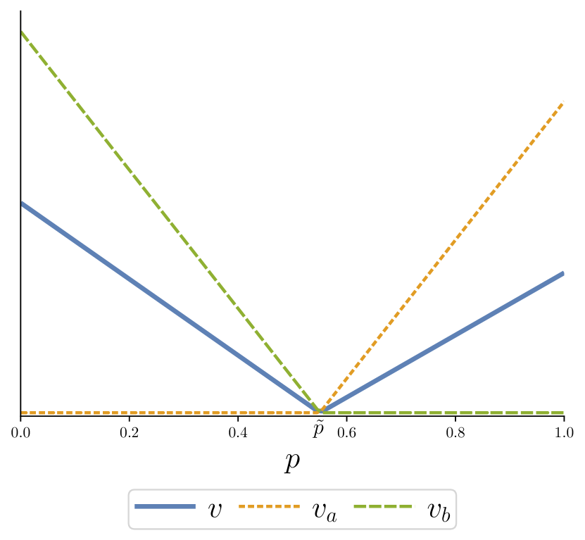
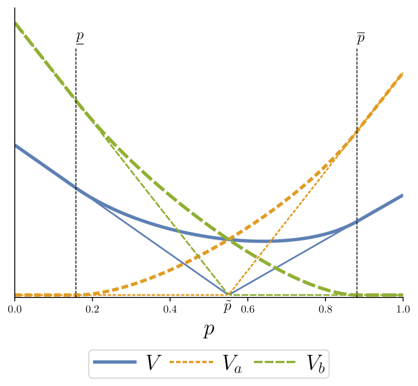
(a) (b) Figure 1: Payoff and Value Functions

In showing that the continuation region is characterised by two constant thresholds, Lemma 2 extends this standard result from Shiryaev (2007) to our slightly more general setting in which the payoff difference between the two alternatives is not certain as in Fudenberg et al. (2018). In other words, it is not the fact that $|u(a,\theta)-u(b,\theta)|$ is constant with respect to $\theta$ that underlies the boundary being constant, but rather that $u(a,\theta)-u(b,\theta)$ takes only two possible values.

This observation is valuable as it makes transparent the connection between our model and the drift-diffusion model. In the standard use of the drift-diffusion model, the decision-maker stops as soon as the accumulated evidence reaches a pre-specified threshold (Forstmann et al., 2016), which is equivalent to the decision-maker stopping as soon as their belief about $\theta$ reaches a pre-specified threshold. While these thresholds and the model parameters are typically estimated from choice data, it is understood that the thresholds are endogenous: “[t]he assumption is that payoffs or instructions induce the subject to adjust the positions of the (…) boundaries and so to adjust the amount of information required for a decision” (Ratcliff, 1978). Our focus is exactly on how problem complexity, $\mu/\sigma$, affects the optimal stopping boundaries, and how this in turn affects the speed and accuracy of choices.

In order to precisely determine the optimal stopping thresholds, we rely on the differential characterisation of the value function $V$:

Lemma 4.

The value function $V$ is given by the unique viscosity solution to the free-boundary problem

$$0 =-c+2(\mu/\sigma)^{2}\left(p(1-p)\right)^{2}V^{\prime\prime}(p) \text{ on }p\in(\underline{p},\overline{p})$$ (HJB)

$$0 =V(p)-v(p) \text{ on }p\notin(\underline{p},\overline{p}).$$ (BC)

Note that $V$ by definition is not a classical solution to the boundary problem since it will necessarily fail to be $\mathcal{C}^{2}$. We then obtain the following characterisation of the optimal stopping boundaries. Denoting the log-odds of $p$ by $\ell(p):=\ln(p/(1-p))$, we then have:

Proposition 1.

The optimal stopping time $\tau^{*}$ is given by $\tau^{*}=\inf\{t\geq 0:p_{t}\notin(\underline{p},\overline{p})\}$, where $\underline{p}$ and $\overline{p}$ are the unique solution to

$$\frac{\left(\frac{\mu}{\sigma}\right)^{2}}{\tilde{c}} =\left[\exp(\overline{\ell})-\exp(-\overline{\ell})+2\overline{\ell}\right]-\left[\exp(\underline{\ell})-\exp(-\underline{\ell})+2\underline{\ell}\right]$$ (1)

$$0 =\left[\overline{\ell}+\exp(\overline{\ell})-\exp(\tilde{\ell})(\overline{\ell}-\exp(-\overline{\ell}))\right]-\left[\underline{\ell}+\exp(\underline{\ell})-\exp(\tilde{\ell})(\underline{\ell}-\exp(-\underline{\ell}))\right]$$ (2)

where $\overline{\ell}:=\ell(\overline{p})$, $\underline{\ell}:=\ell(\underline{p})$, $\tilde{\ell}:=\ell(\tilde{p})$, and $\tilde{c}:=c/(2\delta)$.

The proof of Proposition 1 is but a corollary of Lemma 4: by explicitly solving the free-boundary problem, we obtain the optimal stopping boundaries as the unique solution to (1) and (2).

3.2.  Speed and Accuracy

As indicated, our main result for this section is the following:

Theorem 1.

Accuracy $\mathbb{P}(\alpha_{\tau^{*}}=\theta)$ is increasing in $\mu/\sigma$, and expected optimal stopping time $\mathbb{E}[\tau^{*}]$ is non-monotone and quasi-concave in $\mu/\sigma$, and strictly so for all $\mu/\sigma$ such that $\tau^{*}\neq 0$.

Given the stopping boundaries in log-odds beliefs, $\overline{\ell},\underline{\ell}$, one can translate these to stopping boundaries for the Wiener process, as $\ell_{t}=2(\mu/\sigma^{2})X_{t}$. From there, it is well-known how to obtain closed-form expressions for the expected stopping time and the probability of choosing the best alternative as a function of $\mu/\sigma$. Then, the comparative statics in Theorem 1 arise from a simple, even if cumbersome, application of the implicit function theorem using (1) and (2). Figure 2 exhibits the how speed and accuracy depend on problem complexity and their implied inverse $U$-shaped relationship.

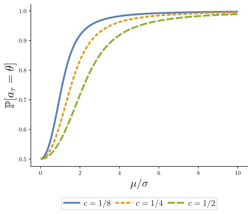
(a)

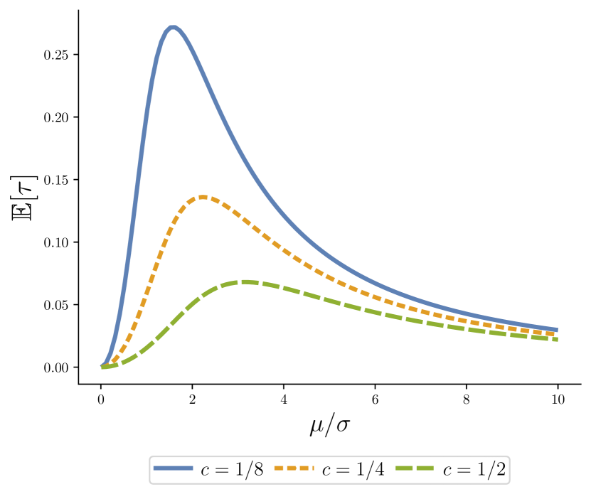
(b)

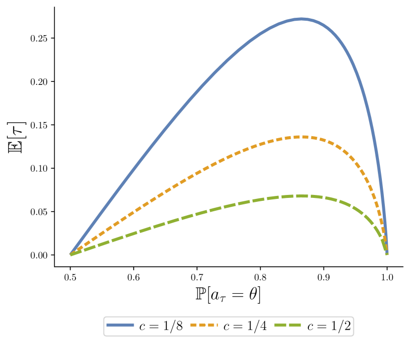
(c)

Figure 2: Speed and Accuracy

Theorem 1 implies that easier problems translate into more accurate choices, which, as the proof shows, is due to wider stopping thresholds for beliefs. While wider thresholds entail longer expected stopping times, a higher signal-to-noise ratio entail faster choices. The former effect dominates for more difficult problems, when the signal-to-noise ratio is low, whereas the latter dominates when simpler problems are made simpler.

This result is consistent with existing evidence that, in simple situations, faster choices are more accurate, but in more complicated ones, the opposite is true (e.g. Achtziger and Alós-Ferrer, 2013).

We want to highlight two common variants of the model that will not affect this observation. In many instances, the drift is proportional to the payoff difference (e.g. Fehr and Rangel, 2011). In our model, this would be observationally equivalent to having a drift rate of $\mu\;\delta$ rather than just $\mu$. Theorem 1 would hold just the same in this case. A second variant of the model would feature exponential discounting instead of a flow cost of time; in Appendix B we show that our results are robust: the relation between accuracy and expected stopping time remains non-monotone.

One important implicit assumption in our analysis is that the decision-maker can to some extent recognise the complexity of the problem they face. In this, we differ from previous literature, e.g. Fudenberg et al. (2018), who preclude this possibility. While it may often be the case that one learns about how complicated a particular problem is while trying to solve it, there may be many instances in which there are apparent differences in complexity across problems, and the decision-maker can realise this. In such cases, without further assumptions, one should not in general expect the speed of decision to indicate response accuracy or problem complexity.

4.  Ability and Effort

We extend our model to speak to effort and ability. Our intent is twofold. First, we wish to acknowledge that time spent is not necessarily a good measure of the effort spent in a task. For instance, a decision-maker might spend a lot of time on a task, but not exert much effort because it is a simple problem, or might spend little time on a hard task but exert a lot of effort. We therefore allow the decision-maker to control how much effort they will exert, positing that more effort is costly but increases how much progress they make per unit of time.

Second, we wish to speak to the ambiguity in the literature regarding the relation between ability and response time. In many contexts slower response times are taken to be indicative of greater ability. For instance, it is often found that individuals who commit more time to a problem tend to be more successful or sophisticated (e.g. Rubinstein, 2016; Agranov et al., 2015; Esteban-Casanelles and Gonçalves, 2022; Gill and Prowse, 2023).

While the studies that relate response time to ability rely on measuring ability from performance independently, one may be tempted to infer ability from response time directly when performance outcomes are ambiguous or not available. Our results suggest that this is not a good idea.

We revisit the model in Section 2 and extend it to allow for the decision-maker to control instantaneous effort $e_{t}\geq 0$, borrowing from Moscarini and Smith (2001). Greater effort translates to more informative signals, formally

$$\mathop{}\!\mathrm{d}X_{t}=\sqrt{e_{t}}\mu\,s(\theta)\mathop{}\!\mathrm{d}t+\sigma\mathop{}\!\mathrm{d}B_{t}.$$

where $\mu,\sigma>0$ are the same as before, $B_{t}$ is a standard Brownian motion, and $e_{t}$ is the instantaneous effort exerted by the decision-maker.

Exerting effort is costly, entailing a cost per unit of time of $c(e/\lambda)\geq 0$, with $c^{\prime},c^{\prime\prime}>0$. The term $\lambda>0$ captures the decision-maker’s ability, with higher values of $\lambda$ capturing lower costs of exerting effort and thus higher ability.

The decision-maker of ability $\lambda$ then chooses a stopping time $\tau$ and a path of effort $(e_{t})$, adapted to the natural filtration induced by $X_{t}$, to maximise their expected payoff,

$$\mathbb{E}_{p_{0}}\left[v(p_{\tau})-\int_{0}^{\tau}c(e_{t}/\lambda)\mathop{}\!\mathrm{d}t\right]$$

with $p_{t}=\mathbb{E}_{p_{0}}[1_{\theta=a}|X_{t}]$ denoting the decision-maker’s posterior belief, $\mathop{}\!\mathrm{d}X_{t}=\sqrt{e_{t}}\mu s(\theta)\mathop{}\!\mathrm{d}t+\sigma\mathop{}\!\mathrm{d}B_{t}$ and $X_{0}=0$.

We find that decision time alone is not a good measure of ability. Specifically, we show that:

Proposition 2.

Let $\lambda_{H}>\lambda_{L}>0$. Then, (1) accuracy is always higher for the high ability type, $\mathbb{P}(\alpha^{*}_{H}=\theta)>\mathbb{P}(\alpha^{*}_{L}=\theta)$, and (2) there are $\overline{k},\underline{k}>0$ such that, for all problems which are sufficiently complex, $\mu/\sigma\leq\underline{k}$, the expected stopping time is higher for the higher ability type $\mathbb{E}[\tau^{*}_{H}]\geq\mathbb{E}[\tau^{*}_{L}]$, and for all simple enough problems, $\mu/\sigma\geq\overline{k}$, the reverse is true. Furthermore, the inequalities are strict whenever $\tau^{*}_{H}\neq 0$.

The proof of Proposition 2 proceeds by observing that, from the HJB equation, optimal effort is constant and, for the optimal effort of a decision-maker with ability $\lambda$, $e_{\lambda}^{*}$, is given by $e^{*}_{\lambda}=\lambda e^{*}_{1}$. Hence, the higher the ability, the greater the effort exerted. This then translates to an effectively higher signal-to-noise ratio, $\sqrt{e^{*}_{\lambda}}\mu/\sigma$, and Proposition 2 then follows from Theorem 1.

We note that Proposition 2 is consistent with recent research in psychology that highlights the importance of taking into account task complexity when interpreting the relation between ability and response time — see e.g. Dodonova and Dodonov (2013), Goldhammer et al. (2014), Kyllonen and Zu (2016), and Junghaenel et al. (2023). In short, these studies find that, in simple tasks, faster responses are indicative of greater ability, but in complex tasks, the opposite is true. Our simple model can rationalise this nuanced prediction.

5.  General Costs of Information Acquisition

We turn to the question of how general this non-monotonic relation between speed and accuracy is when considering a general class of models with costly information acquisition.

Specifically, we consider a decision-maker faces uncertainty about an unknown state $\theta\in\Theta$ and can acquire a Blackwell experiment $\pi$ to learn about $\theta$, which, following existing literature (e.g. Kamenica and Gentzkow, 2011; Caplin et al., 2022; Lipnowski and Ravid, 2023), we model as a distribution over posterior beliefs, i.e. $\pi\in\Pi:=\Delta(\Delta(\Theta))$ such that $\mathbb{E}_{\pi}[p]=p_{0}$. We denote by $C:\Pi\to\overline{\mathbb{R}}$ the cost of the experiment, which we assume is strictly increasing with respect to the Blackwell order $\geq_{B}$, continuous with respect to the Lévy-Prokhorov metric, strictly convex, and normalised such that a fully uninformative experiment bears zero cost, $C(\delta_{p_{0}})=0$. We model the benefit of information as a function $B:\Pi\to\mathbb{R}$ that is bounded, linear, and strictly increasing with respect to the Blackwell order, which arises as the decision-maker’s expected payoff from choosing an action $a\in A$ in order to maximise their expected payoff given posterior beliefs $p\sim\pi$, i.e. $B(\pi)=\mathbb{E}_{\pi}[\max_{a\in A}\mathbb{E}_{p}[u(a,\theta)]]$.

The decision-maker then chooses an experiment in order to maximise their value of information, $v(\pi;\kappa):=B(\pi)-\kappa C(\pi)$, where $\kappa\geq 0$ is a scaling parameter. We denote the value function, optimal experiment, and cost of the optimal experiment as $V(\kappa):=\sup_{\pi\in\Pi}v(\pi;\kappa)$, $\pi^{*}(\kappa):=\arg\max_{\pi\in\Pi}v(\pi;\kappa)$, and $C^{*}(\kappa):=C(\pi^{*}(\kappa))$.

In order to connect this framework to time, we assume that the decision-maker’s expected stopping time is proportional to the total cost of information, i.e. $T^{*}(\kappa):=\mathbb{E}[\tau^{*}]\propto\kappa C^{*}(\kappa)$. The scale $\kappa$ is then interpreted as a measure of problem complexity, scaling the marginal cost of information. In the case of the Wald problem, this is simply reciprocal of the square of the signal-to-noise ratio, $\kappa=(\mu/\sigma)^{-2}$, which extends to a setting with many states (Morris and Strack, 2019).

We then obtain the following result:

Proposition 3.

$T^{*}(\kappa)$ is non-monotone in $\kappa$.

The result follows from a simple application of Berge’s maximum theorem.

Single-peakedness in the general case is more difficult to establish, requiring that $-\kappa V^{\prime\prime}(\kappa)/V^{\prime}(\kappa)$ crosses at most once. Going beyond this loose characterisation requires additional structure.

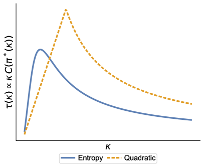
Figure 3: Other Information Costs

Remark 1.

Returning to the binary decision problems introduced in Section 2, we suppose $A=\Theta=\{a,b\}$ and $\tilde{p}=1/2$. If one assumes costs of information are posterior-separable (Caplin et al., 2022), i.e. given by $C(\pi)=\mathbb{E}_{\pi}[c(p)]$ for some $c:[0,1]\to\mathbb{R}_{+}$ satisfying $c^{\prime},c^{\prime\prime}>0$, and $c(p_{0})=0$, then $T^{*}(\kappa)$ is single-peaked if and only if $c(p)/c^{\prime}(p)$ is quasiconcave on $[1/2,1]$.

The argument is simple. First, we recall the well-known result that additively separable information costs, it is without loss of optimally to choose information structures with at most $|A|$ signals, in this case $\overline{p}$ and $\underline{p}$. Symmetry of the problem ($\tilde{p}=p_{0}=1/2$) implies at an optimum $\overline{p}=1-\underline{p}$. The observation follows from the first-order condition $2-\kappa c^{\prime}(p)=0$.

While this implies that single-peakedness of $T^{*}(\kappa)$ is not generic, the most common posterior-based information cost functions do have that $c(p)/c^{\prime}(p)$ is quasiconcave on $[1/2,1]$, e.g. entropy costs, $c(p)=p\ln(p)+(1-p)\ln(1-p)-\ln(1/2)$, and quadratic or variance costs, $c(p)=(p-p_{0})^{2}$ — see Figure 3.

6.  Identifying Complexity

Finally, we turn to the question that often motivates the use of response times in the first place: identifying complexity. As complexity is almost tantamount to mistakes and suboptimal choices, being able to say when a problem is more complex than another is a necessary first step in understanding what makes a problem complex and how to make it simpler (or more complex, depending on the goal). This is well exemplified by many everyday-life situations, going from choosing insurance plans to comparing phone features.

In this section we take the stance of an analyst considering how to assess whether one problem is more or less complex than another. If the analyst knows which choices are optimal, then they can use the decision-maker’s accuracy to infer the complexity of the problem, since more complex problems are associated with lower accuracy. This is the approach often taken in experimental work, where the analyst knows the true state of the world, and the decision-maker’s accuracy is then used to infer the complexity of the problem.

However, in many situations, the analyst does not know which choices are optimal. For instance, suppose that one is interested in assessing which features of a particular mechanism that elicits private information make it more complex. In this case, which choices are optimal will typically depend exactly on the private information the designer is trying to elicit. Furthermore, our earlier results highlight the limitations of using expected response time as a measure of problem complexity. Hence, we would like some behavioural measure that is monotone in complexity that can be easily observed, aggregated across heterogeneous populations, and used to infer the complexity of a problem.

We propose an alternative way forward, which relies on distorting incentives. To be more specific, suppose that our decision-maker in problem $A$ is choosing between alternatives $a$ and $b$ and in problem $\hat{A}$ is choosing between alternatives $\hat{a}$ and $\hat{b}$. In the context of our model, we would say that, all else equal, problem $A$ is more complex than problem $\hat{A}$ if the latter has a higher signal-to-noise ratio, $\hat{\mu}/\hat{\sigma}$, than the former.

Suppose that one could simply pay 1 cent when the decision-maker chooses alternative $b$ in $A$ and $\hat{b}$ in $\hat{A}$. This would marginally increase the decision-maker’s indifference point, $\tilde{p}$, without significantly affecting anything else, and so one would expect $b$ and $\hat{b}$ to be now chosen more often in both problems. What our main result in this section shows is that this small incentive distortion has a greater effect the more complex the problem is.

Theorem 2.

Suppose $\mathbb{P}(\alpha_{\tau}=b)\in(0,1)$. Then $\displaystyle\frac{\partial^{2}}{\partial\tilde{p}\partial(\mu/\sigma)}\mathbb{P}(\alpha_{\tau}=b)<0$.

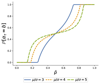
Figure 4: Choice, Problem Complexity, and Payoff Manipulation

Figure 4 clearly illustrates the result: the higher the indifference point $\tilde{p}$, the more likely the decision-maker is to choose $b$. The effect of problem complexity is then to affect how much more the decision-maker is likely to choose $b$ when the indifference point is increased. It is immediate that the more complex the problem is, insofar as the the choice probability is interior, the stronger the dependence of the choices on the indifference point is, and the steeper the lines are. This is captured by the cross-partial derivative $\partial^{2}\mathbb{P}(\alpha_{\tau}=b)/(\partial\tilde{p}\partial(\mu/\sigma))$ being positive. The proof of this fact follows by obtaining a closed-form characterisation of this derivative using implicit differentiation. The important point is that this result is robust to aggregating over heterogenous agents with different preferences, insofar as these are distributed the same across the two problems.

7.  Final Remarks

We believe that our results have important implications for the use of response times in the social sciences. While response times provide an important source of information that is able to shed light on the cognitive processes underlying decision-making, our results support existing evidence that, on their own, they are not a reliable indicator of problem complexity or ability. Instead, we propose to use small incentive distortions to infer problem complexity. These are easy to implement in real-life settings and could be used to study which features make specific problems more or less complex, and evaluate if particular policies improve them. We find these to be promising avenues for future research.

8.  References

Appendix A.  Omitted Proofs

A.1.  Proof of Lemma 1

Proof.

We focus on the $V(p)=\delta V_{a}(p)+u(b,p)$ and $\operatorname*{arg\,max}_{\tau}\mathbb{E}_{p_{0}}[v(p_{\tau})-c\tau]=\operatorname*{arg\,max}_{\tau}\mathbb{E}_{p_{0}}[v_{a}(p_{\tau})-(c/\delta)\tau]$, since the other case is analogous. Note that $u(\alpha,p)=\delta u_{a}(\alpha,p)+u(b,p)$, for $\alpha=a,b$. For any stopping time $\tau$ which is finite almost surely, $\mathbb{E}_{p_{0}}[v(p_{\tau})-c\tau]=\delta\mathbb{E}_{p_{0}}[(p_{\tau}-\tilde{p})^{+}-(c/\delta)\tau]+\mathbb{E}_{p_{0}}[u(b,p_{\tau})]=\delta\mathbb{E}_{p_{0}}[v_{a}(p_{\tau})-(c/\delta)\tau]+\mathbb{E}_{p_{0}}[u(b,p_{\tau})]=\delta\mathbb{E}_{p_{0}}[v_{a}(p_{\tau})-(c/\delta)\tau]+u(b,p_{0})$, where we used optional stopping theorem with the fact that beliefs are a martingale and lie in a compact set. Any optimal stopping time must be finite almost surely, as otherwise the expected value is negative infinity. Hence, $\operatorname*{arg\,max}_{\tau}\mathbb{E}_{p_{0}}[v(p_{\tau})-c\tau]=\operatorname*{arg\,max}_{\tau}\delta\mathbb{E}_{p_{0}}[v_{a}(p_{\tau})-(c/\delta)\tau]+u(b,p_{0})=\operatorname*{arg\,max}_{\tau}\mathbb{E}_{p_{0}}[v_{a}(p_{\tau})-(c/\delta)\tau]$ and $\max_{\tau}\mathbb{E}_{p_{0}}[v(p_{\tau})-c\tau]=\delta\max_{\tau}\mathbb{E}_{p_{0}}[v_{a}(p_{\tau})-(c/\delta)\tau]+u(b,p_{0})=\delta V_{a}(p_{0})+u(b,p_{0})$. ∎

A.2.  Proof of Lemma 2

In text.

A.3.  Proof of Lemma 3

Proof.

We focus on $V_{a}$; the proof for $V_{b}$ is analogous. Let $g=(g_{t})$ denote a stochastic process adapted to the natural filtration induced by $(X_{t})$. Then, note that $V_{a}(p_{0})=\sup_{g,\tau}\mathbb{E}_{p_{0}}[u_{a}(g_{\tau},p_{\tau})-c\tau]$. Letting $W_{a}(p_{0},\tau,g):=\mathbb{E}_{p_{0}}[u_{a}(g_{\tau},p_{\tau})-c\tau]=\mathbb{E}_{p_{0}}[u_{a}(g_{\tau},\theta)-c\tau]$, we have that $V_{a}(p_{0})=\sup_{g,\tau}W_{a}(p_{0},\tau,g)$. Since $W_{a}$ is linear in $p_{0}$, $V_{a}$ is convex in $p_{0}$.

Since $V_{a}\geq v_{a}$, both $V_{a}$ and $v_{a}$ are convex, $v_{a}$ is increasing, and $V_{a}(1)=v_{a}(1)$ and $V_{a}(0)=v_{a}(0)$, we must have that $V_{a}$ is also increasing. ∎

A.4.  Proof of Lemma 4

Proof.

From Lemma 2, there are $0<\underline{p}\leq\overline{p}<1$ such that $\tau^{*}:=\inf\{t\geq 0:p_{t}\notin(\underline{p},\overline{p})\}$. Given this, the fact that $V$ is the unique viscosity solution of the free-boundary problem follows from Øksendal and Reikvam (1998, Proposition 3.1.). ∎

A.5.  Proof of Proposition 1

Proof.

Given Lemma 1, the free-boundary problem can be equivalently given by

$$0 =-\tilde{c}+(\mu/\sigma)^{2}\left(p(1-p)\right)^{2}V_{a}^{\prime\prime}(p) \text{ on }p\in(\underline{p},\overline{p})$$ (HJBa)

$$0 =V_{a}(p)-v_{a}(p) \text{ on }p\in\{\underline{p},\overline{p}\},$$ (BCa)

where $\tilde{c}=c/(2\delta)$ and acknowledging that $V_{a}^{\prime\prime}=V^{\prime\prime}/\delta$.

As $V$ is a viscosity solution of the problem in Lemma 4, on $(\underline{p},\overline{p})$, by definition of the boundaries, $V_{a}>v_{a}$. Moreover, by Lemma 3, $V_{a}$ is convex, and so, by Alexandrov’s theorem, $V_{a}^{\prime\prime}$ exists a.e. and left and right derivatives exist everywhere.

Suppose that $V_{a}$ has a kink at $p\in(\underline{p},\overline{p})$, i.e. $V_{a}^{\prime}(p^{+})\neq V_{a}^{\prime}(p^{-})$. Then, by convexity, $V_{a}^{\prime}(p^{+})>V_{a}^{\prime}(p^{-})$, and, for any $k\in(V_{a}^{\prime}(p^{-}),V_{a}^{\prime}(p^{+}))$ and significantly high $M>0$, $V_{a}(p^{\prime})\geq V_{a}(p)+k(p^{\prime}-p)+(M/2)(p^{\prime}-p)^{2}=:\psi(p^{\prime})$ for $p^{\prime}$ in a neighborhood of $p$. Then, we would obtain that $\tilde{c}-(\mu/\sigma)^{2}(p(1-p))^{2}M<0$ for sufficiently high $M$, contradicting the fact that $V_{a}$ is a viscosity supersolution. Hence, $V_{a}$ is $\mathcal{C}^{1}$ except possibly at $\{\underline{p},\overline{p}\}$.

Since $V_{a}^{\prime\prime}$ exists a.e., from Crandall et al. (1992, p. 15), the HJB will hold with equality whenever $V_{a}$ is twice differentiable, i.e. almost everywhere on $(\underline{p},\overline{p})$. Furthermore, $0\leq V_{a}^{\prime\prime}\leq(\mu/\sigma)^{-2}\tilde{c}\max\{(\underline{p}(1-\underline{p}))^{-2},(\overline{p}(1-\overline{p}))^{-2}\}$, and so $V_{a}^{\prime\prime}$ is bounded whenever it exists. Take any sequence $(p_{n})\subset(\underline{p},\overline{p})$ such that $p_{n}\to p^{*}\in(\underline{p},\overline{p})$. Then, there is a subsequence $(p_{m})$ such that $V_{a}^{\prime}(p_{m})\to V_{a,\infty}^{\prime}$, $V_{a}^{\prime\prime}(p_{m})\to V_{a,\infty}^{\prime\prime}$, and, by continuity, $0=-\tilde{c}+(\mu/\sigma)^{2}\left(p^{*}(1-p^{*})\right)^{2}V_{a,\infty}^{\prime\prime}$. Hence $(V_{a,\infty}^{\prime},V_{a,\infty}^{\prime\prime})$ belongs to both the super- and subjet of $V_{a}$ at $p^{*}$, implying that $V_{a}$ is twice continuously differentiable everywhere except possibly at $\{\underline{p},\overline{p}\}$.

Then, for some $\beta_{0},\beta_{1}\in\mathbb{R}$ to be determined

$$V_{a}(p) =\frac{\tilde{c}}{(\mu/\sigma)^{2}}\frac{\exp(\ell(p))-1}{\exp(\ell(p))+1}\ell(p)+\frac{\exp(\ell(p))}{\exp(\ell(p))+1}\beta_{1}+\beta_{0},$$

$$V_{a}^{\prime}(p) =\frac{\tilde{c}}{(\mu/\sigma)^{2}}\left(\exp(\ell(p))-\exp(-\ell(p))+2\ell(p)\right)+\beta_{1}.$$

As the optimal stopping time is finite almost surely, $0<\underline{p}\leq\overline{p}<1$ and so $V_{a}^{\prime\prime}(\underline{p}^{+}),V_{a}^{\prime\prime}(\overline{p}^{-})>0=v_{a}^{\prime\prime}(p)$ $\forall p\neq\tilde{p}$, which implies that the boundary condition is binding at the boundaries and therefore $V_{a}\in\mathcal{C}^{0}([0,1])$ and convex.

We guess and verify that $V\in\mathcal{C}^{1}([0,1])$. From $V_{a}^{\prime}(\underline{p}^{+})=v_{a}^{\prime}(\underline{p}^{-})=0$ and $V_{a}^{\prime}(\overline{p}^{-})=v_{a}^{\prime}(\overline{p}^{+})=1$, one obtains $-\beta_{1}=\frac{\tilde{c}}{(\mu/\sigma)^{2}}\left(\exp(\underline{\ell})-\exp(-\underline{\ell})+2\underline{\ell}\right)=\frac{\tilde{c}}{(\mu/\sigma)^{2}}\left(\exp(\overline{\ell})-\exp(-\overline{\ell})+2\overline{\ell}\right)-1$, from which (1) follows. Then,

$$0=V_{a}(\underline{p})-v_{a}(\underline{p}) =\frac{\tilde{c}}{(\mu/\sigma)^{2}}\left((1-\exp(\underline{\ell}))-\underline{\ell}\right)+\beta_{0},$$

$$0=V_{a}(\overline{p})-v_{a}(\overline{p}) =\frac{\tilde{c}}{(\mu/\sigma)^{2}}\left((1-\exp(\overline{\ell}))-\overline{\ell}\right)+\beta_{0}+\tilde{p},$$

which yields

$$\left((1-\exp(\underline{\ell}))-\underline{\ell}\right)-\left((1-\exp(\overline{\ell}))-\overline{\ell}\right)=\frac{(\mu/\sigma)^{2}}{\tilde{c}}\tilde{p}.$$

Replacing $\frac{(\mu/\sigma)^{2}}{\tilde{c}}$ with (1) and rearranging the expression delivers (2).

Given $\underline{\ell}\leq\overline{\ell}$, (2) implies $\underline{\ell}\leq\tilde{\ell}\leq\overline{\ell}$. Then, both (1) and (2) implicitly define $\underline{\ell}$ as a function of $\overline{\ell}$, which we denote by $\underline{\ell}_{1}(\cdot)$ and $\underline{\ell}_{2}(\cdot)$, respectively. From the implicit function theorem, we obtain that $\underline{\ell}_{1}$ is strictly increasing and $\underline{\ell}_{2}$ strictly decreasing. Moreover, $\underline{\ell}_{2}(\tilde{\ell})=\tilde{\ell}$, whereas since the right-hand side of (1) is decreasing in $\underline{\ell}$ and that it is zero for $\underline{\ell}=\overline{\ell}$, we obtain that $\underline{\ell}_{1}(\tilde{\ell})<\tilde{\ell}$. Additionally, straightforward manipulation of (1) and (2) shows that for some large enough $\overline{\ell}$, $\underline{\ell}_{1}(\overline{\ell})>0>\underline{\ell}_{2}(\overline{\ell})$, hence there is a unique $\overline{\ell}$ such that $\underline{\ell}_{1}(\overline{\ell})=\underline{\ell}_{2}(\overline{\ell})$. This shows that the system formed by (1) and (2) does have a (unique) solution $(\underline{\ell},\overline{\ell})$ such that $\underline{\ell}\leq\tilde{\ell}\leq\overline{\ell}$, thus verifying the conjecture that $V_{a}\in\mathcal{C}^{1}([0,1])$ and concluding the proof. ∎

A.6.  Proof of Theorem 1

Proof.

We focus on the case in which $\tilde{p},p_{0}\in(\underline{p},\overline{p})$, since if this were not the case, the decision-maker with prior $p_{0}$ would prefer to stop immediately.

Letting $\ell(p):=\ln(p/(1-p))$, we first note that the information process $X_{t}$ induces a process for log-odds beliefs given by $\ell_{t}:=2\frac{\mu}{\sigma^{2}}X_{t}$. Second, we observe that, given $\theta$, $\exp(-(2s(\theta)\mu/\sigma^{2})X_{t})$ is a martingale and as $X_{\tau}$ is therefore bounded, we can apply the optional stopping theorem (Ethier and Kurtz, 2005, Ch. 2, Theorem 2.3) to obtain $1=\exp(-(2s(\theta)\mu/\sigma^{2})X_{0})=\mathbb{E}[\exp(-(2s(\theta)\mu/\sigma^{2})X_{\tau})\mid\theta]=\mathbb{E}[\exp(-s(\theta)\ell_{\tau})\mid\theta]$.

Recall that $\overline{\ell}:=\ell(\overline{p})$, $\underline{\ell}:=\ell(\underline{p})$, and $\tilde{\ell}:=\ell(\tilde{p})$. As $\mathbb{P}(\alpha_{\tau}=a\mid\theta)=\mathbb{P}(\ell_{\tau}=\overline{\ell}\mid\theta)=1-\mathbb{P}(\ell_{\tau}=\underline{\ell}\mid\theta)$ and $\mathbb{E}[\exp(-s(\theta)\ell_{\tau})\mid\theta]=\mathbb{P}(\ell_{\tau}=\overline{\ell}\mid\theta)\exp(-s(\theta)\overline{\ell})+\mathbb{P}(\ell_{\tau}=\underline{\ell}\mid\theta)\exp(-s(\theta)\underline{\ell})$, we have $\mathbb{P}(\alpha_{\tau}=\theta)=\frac{1}{2}(\mathbb{P}(\alpha_{\tau}=a\mid\theta=a)+\mathbb{P}(\alpha_{\tau}=b\mid\theta=b))=\frac{1}{2}\left(\exp(\overline{\ell})\frac{1-\exp(\underline{\ell})}{\exp(\overline{\ell})-\exp(\underline{\ell})}+\frac{\exp(\overline{\ell})-1}{\exp(\overline{\ell})-\exp(\underline{\ell})}\right)$. $\mathbb{P}(\alpha_{\tau}=\theta)$ is strictly increasing in $\overline{\ell}$ and decreasing in $\underline{\ell}$. A straightforward application of the implicit function theorem to the system formed by (1) and (2) reveals that $(\overline{\ell},-\underline{\ell})$ is increasing in $\mu/\sigma$, implying that accuracy, $\mathbb{P}(\alpha_{\tau}=\theta)$, is increasing in $\mu/\sigma$.

We then use Wald’s identity to obtain $\mathbb{E}[\ell_{\tau}\mid\theta]=2\left(\frac{\mu}{\sigma}\right)^{2}s(\theta)\mathbb{E}[\tau\mid\theta]$. As $\mathbb{E}[\ell_{\tau}\mid\theta]=\mathbb{P}(\ell_{\tau}=\overline{\ell}\mid\theta)\overline{\ell}+\mathbb{P}(\ell_{\tau}=\underline{\ell}\mid\theta)\underline{\ell}$, we then obtain

$$\mathbb{E}[\tau] =\frac{1}{4(\mu/\sigma)^{2}}\left(\mathbb{P}(\ell_{\tau}=\overline{\ell}\mid\theta=a)-\mathbb{P}(\ell_{\tau}=\overline{\ell}\mid\theta=b)\right)(\overline{\ell}-\underline{\ell})$$

$$=\frac{1}{4(\mu/\sigma)^{2}}\frac{(1-\exp(\underline{\ell}))(\exp(\overline{\ell})-1)}{\exp(\overline{\ell})-\exp(\underline{\ell})}(\overline{\ell}-\underline{\ell}).$$ (3)

Replacing $(\mu/\sigma)^{2}$ in (3) with (1) and taking logs we obtain $T(\overline{\ell},\underline{\ell})$, a strictly concave function of $(\overline{\ell},\underline{\ell})\in\mathbb{R}_{+}\times\mathbb{R}_{-}$, satisfying $T(\overline{\ell},\underline{\ell})=T(-\underline{\ell},-\overline{\ell})$. $T$ therefore encodes the dependence of the stopping thresholds on $\mu/\sigma$, but not the optimal relation between the upper and lower stopping thresholds, dictated by the indifference point $\tilde{p}$, in its log-odds form $\tilde{\ell}$ in (2).

Since, $\overline{\ell}\downarrow 0$ or $\overline{\ell}\uparrow+\infty$ (resp. $\underline{\ell}\uparrow 0$ or $\underline{\ell}\downarrow-\infty$) implies $\exp(T(\overline{\ell},\underline{\ell}))\downarrow 0$ for any $\underline{\ell}<0$ (resp. $\overline{\ell}>0$), and as $\exp(T(\overline{\ell},\underline{\ell}))>0$ for some $\overline{\ell}>0>\underline{\ell}$, we have that the expected optimal stopping time is non-monotone.

Without loss of generality, we assume $\tilde{p}\geq 1/2$ (as the other case is symmetric), which implies $\overline{\ell}>\tilde{\ell}>\underline{\ell}$. Then, from (2), it is immediate that $\overline{\ell}\geq\tilde{\ell}-\underline{\ell}\geq\tilde{\ell}\geq\ell_{0}=0\geq\underline{\ell}$.

We then rearrange (2) so as to obtain

$$\exp(\tilde{\ell})=\frac{(\overline{\ell}-\underline{\ell})+(\exp(\overline{\ell})-\exp(\underline{\ell}))}{(\overline{\ell}-\underline{\ell})+(\exp(\overline{\ell})-\exp(\underline{\ell}))\exp(-\overline{\ell}-\underline{\ell})},$$ (4)

implicitly defining $\underline{\ell}$ as a function of $\overline{\ell}$. Let $L:\overline{\ell}\mapsto L(\overline{\ell})=(\overline{\ell},\underline{\ell}(\overline{\ell}))$.

Then,

$$\frac{\mathop{}\!\mathrm{d}^{2}}{(\mathop{}\!\mathrm{d}\overline{\ell})^{2}}T(\overline{\ell},\underline{\ell}(\overline{\ell}))=(D_{\overline{\ell}}L(\overline{\ell}))^{T}\cdot D^{2}_{(\overline{\ell},\underline{\ell})}T(\overline{\ell},\underline{\ell})\cdot D_{\overline{\ell}}L(\overline{\ell})+D^{2}_{\overline{\ell}}L(\overline{\ell})\cdot D_{(\overline{\ell},\underline{\ell})}T(\overline{\ell},\underline{\ell})\bigg{|}_{\underline{\ell}=L(\overline{\ell})},$$

where $D_{x}f$ and $D^{2}_{x}f$ denote the first- and second-order derivatives of $f$ with respect to $x$. Note that $D_{\overline{\ell}}L(\overline{\ell})$ and $D^{2}_{\overline{\ell}}L(\overline{\ell})$ are obtained via the implicit function theorem from (4). A straightforward but tedious exercise in examining $\frac{\mathop{}\!\mathrm{d}^{2}}{(\mathop{}\!\mathrm{d}\overline{\ell})^{2}}T(\overline{\ell},\underline{\ell}(\overline{\ell}))$ reveals that it is strictly negative for all $\overline{\ell},\underline{\ell}:\overline{\ell}>0>\underline{\ell}>-\overline{\ell}$, thus showing that the expected optimal stopping time, taken as a function of $\overline{\ell}$, is strictly log-concave in $\overline{\ell}\geq 0$.

We recall that, by the implicit function theorem, using (1) and (2), $(\overline{\ell},-\underline{\ell})$ is increasing in $\mu/\sigma$. Hence, we conclude that the expected optimal stopping time, $\mathbb{E}[\tau^{*}]$, is non-monotone and quasiconcave in $\mu/\sigma$, and strictly so for all $\mu/\sigma$ such that $\tau^{*}\neq 0$. ∎

A.7.  Proof of Proposition 2

Proof.

We first note that the optimal effort for agent $i$, $e_{i}^{*}$, is constant over time and equal to $e^{*}_{i}=\lambda_{i}e^{*}$, where $e^{*}$ is such that $e^{*}c^{\prime}(e^{*})=c(e^{*})$. Write $c_{i}(e_{i}):=c(e_{i}/\lambda_{i})$. The argument (already in Moscarini and Smith (2001)) is that, on the continuation region, the HJB equation is given by

$$0=\sup_{e_{i}>0}\left\{-c_{i}(e_{i})+e_{i}2(\mu/\sigma)^{2}(p(1-p))^{2}V^{\prime\prime}(p)\right\}.$$

The first-order condition yields $e_{i}c_{i}^{\prime}(e_{i})=e_{i}2(\mu/\sigma)^{2}(p(1-p))^{2}V^{\prime\prime}(p)$, whereas the HJB equation implies $c_{i}(e_{i})=e_{i}2(\mu/\sigma)^{2}(p(1-p))^{2}V^{\prime\prime}(p)$. Observe that $e_{i}c_{i}^{\prime}(e_{i})=c_{i}(e_{i})$ has unique solution and so effort is constant over time (while not stopping).

We then have $e_{i}c_{i}^{\prime}(e_{i})=c_{i}(e_{i})\Longleftrightarrow\,\,e_{i}/\lambda_{i}c^{\prime}(e_{i}/\lambda_{i})=c(e_{i}/\lambda_{i})$, which implies $e_{i}=\lambda_{i}e^{*}$ and $c_{i}(e_{i})=c(e_{i}/\lambda_{i})=c(e^{*})$.

Hence, it is as if the decision-maker faces a problem with a constant drift term $\mu_{i}\equiv\sqrt{\lambda_{i}e^{*}}\mu$ and a constant flow cost $c(e^{*})$, and so will have constant stopping thresholds as before.

As accuracy is increasing in the signal-to-noise ratio, we have that the higher ability type will always choose better, as they have a higher effective signal-to-noise ratio, $\mu_{H}/\sigma=\sqrt{\lambda_{H}e^{*}}\mu/\sigma$. In contrast, from Theorem 1, the expected stopping time is single-peaked; let its maximum be attained at $k^{*}$. Defining $\overline{k}:=k^{*}{(\lambda_{L}e^{*})}^{-1/2}$ and $\underline{k}:=k^{*}{(\lambda_{H}e^{*})}^{-1/2}$, the result follows immediately. The restriction $\tau^{*}_{H}\neq 0$ guarantees that we are in the part of the domain of $\lambda_{H}$ and thus signal-to-noise ratio in which the expected stopping time is strictly quasi-concave (ensuring that the stopping thresholds of the high type are bounded away from $0$ and the indifference point). ∎

A.8.  Proof of Theorem 2

Proof.

From the proof of Theorem 1, we have that $\mathbb{P}(\alpha_{\tau}=a\mid\theta)=\mathbb{P}(\ell_{\tau}=\overline{\ell}\mid\theta)$ and $\mathbb{E}[\exp(-s(\theta)\ell_{\tau})\mid\theta]=\mathbb{P}(\ell_{\tau}=\overline{\ell}\mid\theta)\exp(-s(\theta)\overline{\ell})+\mathbb{P}(\ell_{\tau}=\underline{\ell}\mid\theta)\exp(-s(\theta)\underline{\ell})$.

Consequently, $\mathbb{P}(\alpha_{\tau}=a)=\frac{(1+\exp(\overline{\ell}))(1-\exp(\underline{\ell}))}{2(\exp(\overline{\ell})-\exp(\underline{\ell}))}=:q(\overline{\ell},\underline{\ell})$.

From (1) and (4), using the implicit function theorem, we obtain $\frac{\partial}{\partial\exp(\tilde{\ell})}q(\overline{\ell},\underline{\ell})$ as a function $q_{\tilde{\ell}}$ of $\overline{\ell}$ and $\underline{\ell}$, where

$$q_{\tilde{\ell}}(\overline{\ell},\underline{\ell}):=\frac{\partial}{\partial\exp(\tilde{\ell})}q(\overline{\ell},\underline{\ell})=\frac{\partial}{\partial\overline{\ell}}q(\overline{\ell},\underline{\ell})\frac{\partial}{\partial\exp(\tilde{\ell})}\overline{\ell}+\frac{\partial}{\partial\underline{\ell}}q(\overline{\ell},\underline{\ell})\frac{\partial}{\partial\exp(\tilde{\ell})}\underline{\ell}$$

$$=\frac{\exp(-5\overline{\ell}/2-2\underline{\ell})(1+\exp(\overline{\ell}))\left(\exp(\overline{\ell})-\exp(\underline{\ell})+\exp(\overline{\ell}+\underline{\ell})(\overline{\ell}-\underline{\ell})\right)^{2}\text{csch}((\overline{\ell}-\underline{\ell})/2)\text{sech}(\underline{\ell}/2)\text{sinh}(\overline{\ell})}{16(1-\text{cosh}(\overline{\ell}-\underline{\ell}))(\overline{\ell}-\underline{\ell}+\text{sinh}(\overline{\ell})-\text{sinh}(\underline{\ell}))}$$

$$+\frac{\exp(-5\underline{\ell}/2-2\overline{\ell})(1+\exp(\underline{\ell}))\left(\exp(\overline{\ell})-\exp(\underline{\ell})+\exp(\overline{\ell}+\underline{\ell})(\overline{\ell}-\underline{\ell})\right)^{2}{\text{csch}((\overline{\ell}-\underline{\ell})/2)}^{3}\text{sech}(\overline{\ell}/2)\text{sinh}(\underline{\ell})}{32(\overline{\ell}-\underline{\ell}+\text{sinh}(\overline{\ell})-\text{sinh}(\underline{\ell}))},$$

which, as expected, can be shown to be strictly negative for all $\overline{\ell}>0>\underline{\ell}$. Relying again on implicit differentiation, we obtain an explicit characterisation of the cross-partial derivative, $q_{\tilde{\ell},\mu/\sigma}:=\frac{\partial^{2}}{\partial\exp(\tilde{\ell})\partial((\mu/\sigma)^{2})}q=\frac{\partial}{\partial\overline{\ell}}q_{\tilde{\ell}}\frac{\partial}{\partial(\mu/\sigma)^{2}}\overline{\ell}+\frac{\partial}{\partial\underline{\ell}}q_{\tilde{\ell}}\frac{\partial}{\partial((\mu/\sigma)^{2})}\underline{\ell}$, involving exclusively $\overline{\ell},\underline{\ell}$. With a careful examination of the resulting function and extremely tedious algebra it can be shown that $q_{\tilde{\ell},\mu/\sigma}>0$ for all $\overline{\ell}>0>\underline{\ell}$.

As $\mu/\sigma>0$, $\exp(\tilde{\ell})$ and $(\mu/\sigma)^{2}$ are strictly increasing functions of $\mu/\sigma$ and $\tilde{p}$, respectively, and so this implies that $\displaystyle\frac{\partial^{2}}{\partial\tilde{p}\partial(\mu/\sigma)}\mathbb{P}(\alpha_{\tau}=a)>0\Longleftrightarrow\frac{\partial^{2}}{\partial\tilde{p}\partial(\mu/\sigma)}\mathbb{P}(\alpha_{\tau}=b)<0$. ∎

A.9.  Proof of Proposition 3

Proof.

Let $\pi_{I}$ denote a fully informative experiment — i.e. assigning probability $p_{0}(\theta)$ to posterior belief $1_{\theta}$ — and $\pi_{U}$ a fully uninformative experiment, assigning probability 1 to the prior $p_{0}$. Take any $\overline{C}>0$ such that $\exists\overline{\kappa}$ such that $\overline{\kappa}C^{*}(\overline{\kappa})>\overline{C}$. Then, there are $\kappa<\overline{\kappa}$ and $\kappa^{\prime}>\overline{\kappa}$ such that $\kappa C^{*}(\kappa)\vee\kappa^{\prime}C^{*}(\kappa^{\prime})<\overline{C}$. To see this note that, by Berge’s maximum theorem, $\kappa C^{*}(\kappa)$ is continuous in $\kappa$. Taking $\kappa_{n}\downarrow 0$, $V(\kappa_{n})\uparrow V(0)=B(\pi_{I})$, and so $V(0)-V(\kappa_{n})=\kappa_{n}C^{*}(\kappa_{n})\downarrow 0$. Take now $\kappa_{n}\uparrow\infty$. Note that $0\leq\lim_{n\to\infty}V(\kappa_{n})/\kappa_{n}=\lim_{n\to\infty}B(\pi^{*}(\kappa_{n}))/\kappa_{n}-C^{*}(\kappa_{n})=\lim_{n\to\infty}-C^{*}(\kappa_{n})\leq 0$, and so it must be that $\pi^{*}(\kappa_{n})\to\pi_{U}$. Consequently, $\kappa_{n}C^{*}(\kappa_{n})\leq B(\pi^{*}(\kappa_{n}))\to 0$, a contradiction. ∎

Appendix B.  Discounting

In this appendix, we consider a variation of the problem in Section 2 in which the decision-maker, instead of bearing an explicit cost of time, exponentially discounts payoffs at a rate $r>0$. We make the simplifying assumption that $u(\alpha,\theta)=1_{\alpha=\theta}$.

Formally, the decision-maker chooses a stopping time $\tau$ and a stochastic process $(\alpha_{t})$ taking values in $A$, both adapted to the natural filtration induced by the stochastic process$(X_{t})$ in order to maximise their expected payoff, $\mathbb{E}_{p_{0}}\left[\exp(-r\tau)(1_{\alpha_{\tau}=\theta})\right]$, where $p_{t}$ denotes the posterior belief about $\theta$ given $X_{t}$, and $v(p):=\max\{p,1-p\}$. Denote their value function by

$$V(p_{0})=\sup_{\tau}\mathbb{E}_{p_{0}}\left[\exp(-r\tau)(1_{\alpha_{\tau}=\theta})\right].$$

The earliest optimal stopping time is then given by $\tau^{*}:=\inf\{t\geq 0|V(p_{t})\leq v(p_{t})\}$. Let $D:=\{p\in[0,1]:V(p)>v(p)\}$. Since $v,V$ are convex in $p$ and $V(p)=v(p)$ for $p\in\{0,1\}$, and $v$ is piecewise-linear, $D$ must be connected. Letting $\underline{p}:=\inf D$ and $\overline{p}:=\sup D$, we have that $V(p)=v(p)$ for $p\leq\underline{p}$ and $V(p)=v(p)$ for $p\geq\overline{p}$.

Furthermore, since payoffs are symmetric (i.e. $u(a,a)-u(b,a)=u(b,b)-u(a,b)$ and $u(a,b)=u(b,a)$), the stopping thresholds will also be symmetric around $1/2$, i.e. $\underline{p}=1-\overline{p}$. Then,

$$\mathbb{E}_{p_{0}}[\exp(-r\tau^{*})(1_{\alpha_{\tau^{*}}=\theta})]=\mathbb{E}_{p_{0}}[\exp(-r\tau^{*})(1_{\alpha_{\tau^{*}}=\theta})|\theta=a]=\frac{1}{2}\exp\left(\frac{\overline{\ell}}{2}\right)\text{sech}\left(\frac{\overline{\ell}}{2}\;\kappa\right)$$

where the last equality follows from Borodin and Salminen (2002, p. 309, 3.0.5(b)) and $\kappa:={(2r(\sigma/\mu)^{2}+1)}^{1/2}$.

Taking first-order conditions, we get that the optimal stopping boundary is given by $\overline{\ell}^{*}=2\,\text{tanh}^{-1}(1/\kappa)/\kappa.$ It is then immediate that accuracy, $\mathbb{P}(\alpha_{\tau^{*}}=\theta)=(1+\exp(-\overline{\ell}^{*}))^{-1}$, is increasing in $\mu/\sigma$. The expected stopping time fixing $\overline{\ell}=-\underline{\ell}$ is known and given by (3), that is, $\mathbb{E}[\tau]=\frac{\overline{\ell}\,\tanh\left(\overline{\ell}/2\right)}{2(\mu/\sigma)^{2}}.$ Substituting for the optimal stopping threshold $\overline{\ell}^{*}$, we have $\mathbb{E}[\tau^{*}]=\frac{\kappa^{2}-1}{\kappa r}\,\text{coth}^{-1}(\kappa)\,\text{tanh}\left(\text{coth}^{-1}(\kappa)/\kappa\right),$ which is inverse $U$-shaped in $\mu/\sigma$, with $\lim_{\mu/\sigma\downarrow 0}\mathbb{E}[\tau^{*}]=\lim_{\mu/\sigma\uparrow\infty}\mathbb{E}[\tau^{*}]=0$ — see Figure 5.

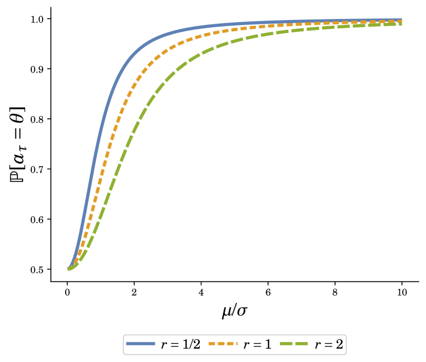
(a)

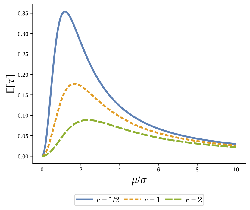
(b)

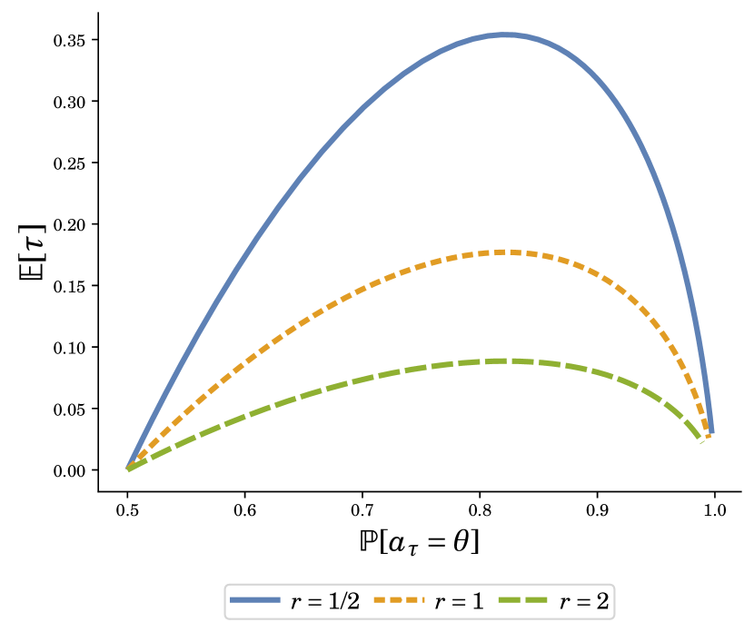
(c)

Figure 5: Speed and Accuracy: Discounting

References

- (1)
- Achtziger and Alós-Ferrer (2013) Achtziger, A., and C. Alós-Ferrer. 2013. “Fast or Rational? A Response-Times Study of Bayesian Updating.” Management Science 60 (4): 923–938. 10.1287/mnsc.2013.1793.
- Agarwal et al. (2016) Agarwal, S., R. J. Rosen, and V. Yao. 2016. “Why Do Borrowers Make Mortgage Refinancing Mistakes?” Management Science 62 (12): 3494–3509. 10.1287/mnsc.2015.2272.
- Agranov et al. (2015) Agranov, M., A. Caplin, and C. Tergiman. 2015. “Naive play and the process of choice in guessing games.” Journal of the Economic Science Association 1 146–157. 10.1007/s40881-015-0003-5.
- Alós-Ferrer (2018) Alós-Ferrer, C. 2018. “A Dual-Process Diffusion Model.” Journal of Behavioral Decision Making 31 203–218. 10.1002/bdm.1960.
- Alós-Ferrer et al. (2021) Alós-Ferrer, C., E. Fehr, and N. Netzer. 2021. “Time Will Tell: Recovering Preferences When Choices Are Noisy.” Journal of Political Economy 129 (6): 1828–1877. 10.1086/713732.
- Alós-Ferrer and Garagnani (2022) Alós-Ferrer, C., and M. Garagnani. 2022. “Strength of preference and decisions under risk.” Journal of Risk and Uncertainty 64 309–329. 10.1007/s11166-022-09381-0.
- Banovetz and Oprea (2023) Banovetz, J., and R. Oprea. 2023. “Complexity and Procedural Choice.” American Economic Journal: Microeconomics 15 (2): 384–413. 10.1257/mic.20210032.
- Bhargava et al. (2017) Bhargava, S., G. Loewenstein, and J. Sydnor. 2017. “Choose to Lose: Health Plan Choices from a Menu with Dominated Option.” Quarterly Journal of Economics 132 (3): 1319–1372. 10.1093/qje/qjx011.
- Bobtcheff and Levy (2017) Bobtcheff, C., and R. Levy. 2017. “More Haste, Less Speed? Signaling through Investment Timing.” American Economic Journal: Microeconomics 9 (3): 148–186. 10.1257/mic.20160200.
- Bogacz et al. (2010) Bogacz, R., E.-J. Wagenmakers, B. Forstmann, and S. Nieuwenhuis. 2010. “The neural basis of the speed-accuracy tradeoff.” Trends in Neurosciences 33 (1): 10–16. 10.1016/j.tins.2009.09.002.
- Börgers and Li (2019) Börgers, T., and J. Li. 2019. “Strategically Simple Mechanisms.” Econometrica 87 (6): 2003–2035. 10.3982/ECTA15897.
- Borodin and Salminen (2002) Borodin, A. N., and P. Salminen. 2002. Handbook of Brownian Motion Facts and Formulae. Springer, , 2nd edition.
- Branco et al. (2012) Branco, F., M. Sun, and J. Villas-Boas. 2012. “Optimal Search for Product Information.” Management Science 58 (11): 2037–2056. 10.1287/mnsc.1120.1535.
- Callander (2011) Callander, S. 2011. “Searching and Learning by Trial and Error.” American Economic Review 111 (6): 2277–2308. 10.1257/aer.101.6.2277.
- Caplin et al. (2020) Caplin, A., D. Csaba, J. Leahy, and O. Nov. 2020. “Rational Inattention, Competitive Supply, and Psychometrics.” Quarterly Journal of Economics 135 (3): 1681–1724. 10.1093/qje/qjaa011.
- Caplin and Dean (2015) Caplin, A., and M. Dean. 2015. “Revealed Preference, Rational Inattention, and Costly Information Acquisition.” American Economic Review 105 (7): 2183–2203. 10.1257/aer.20140117.
- Caplin et al. (2022) Caplin, A., M. Dean, and J. Leahy. 2022. “Rationally Inattentive Behavior: Characterizing and Generalizing Shannon Entropy.” Journal of Political Economy 130 (6): 1–40. 10.1086/719276.
- Caplin and Martin (2016) Caplin, A., and D. Martin. 2016. “Decision Times Reveal Private Information in Strategic Settings: Evidence from Bargaining Experiments.” Economic Inquiry 54 (2): 1274–1282. 10.1111/ecin.12294.
- Carvalho and Silverman (2017) Carvalho, L., and D. Silverman. 2017. “Complexity and Sophistication.” Working Paper 1–47.
- Choi et al. (2011) Choi, J. J., D. Laibson, and B. C. Madrian. 2011. “$100 Bills on the Sidewalk: Suboptimal Investment in 401(k) Plans.” Review of Economics and Statistics 93 (3): 748–763. 10.1162/REST_a_00100.
- Clithero (2018) Clithero, J. 2018. “Improving out-of-sample predictions using response times and a model of the decision process.” Journal of Economic Behavior and Organization 148 344–375. 10.1016/j.jebo.2018.02.007.
- Crandall et al. (1992) Crandall, M. G., H. Ishii, and P.-L. Lions. 1992. “User’s Guide to Viscosity Solutions of Second Order Partial Differential Equations.” Bulletin of the American Mathematical Society 27 1–67. 10.1090/S0273-0979-1992-00266-5.
- Dodonova and Dodonov (2013) Dodonova, Y. A., and Y. S. Dodonov. 2013. “Faster on easy items, more accurate on difficult ones: Cognitive ability and performance on a task of varying difficulty.” Intelligence 41 (1): 1–10. 10.1016/j.intell.2012.10.003.
- Dvoretzky et al. (1953) Dvoretzky, A., J. Kiefer, and J. Wolfowitz. 1953. “Sequential Decision Problems for Processes with Continuous time Parameter. Testing Hypotheses.” Annals of Mathematical Statistics 24 (2): 254–264. 10.1214/aoms/1177729031.
- Ellison and Wolitzky (2012) Ellison, G., and A. Wolitzky. 2012. “A Search Cost Model of Obfuscation.” RAND Journal of Economics 43 (3): 417–441. 10.1111/j.1756-2171.2012.00180.x.
- Enke (2020) Enke, B. 2020. “What You See Is All There Is.” Quarterly Journal of Economics 135 (3): 1363–1398. 10.1093/qje/qjaa012.
- Esteban-Casanelles and Gonçalves (2022) Esteban-Casanelles, T., and D. Gonçalves. 2022. “The Effect of Incentives on Choices and Beliefs in Games: An Experiment.” Working Paper.
- Ethier and Kurtz (2005) Ethier, S. N., and T. G. Kurtz. 2005. Markov Processes: Characterization and Convergence. John Wiley & Sons, Inc..
- Fehr and Rangel (2011) Fehr, E., and A. Rangel. 2011. “Neuroeconomic Foundations of Economic Choice—Recent Advances.” Journal of Economic Perspectives 25 (4): 3–30. 10.1257/jep.25.4.3.
- Forstmann et al. (2016) Forstmann, B., R. Ratcliff, and E.-J. Wagenmakers. 2016. “Sequential Sampling Models in Cognitive Neuroscience: Advantages, Applications, and Extensions.” Annual Review of Psychology 67 (1): 641–666. 10.1146/annurev-psych-122414-033645.
- Frydman and Jin (2022) Frydman, C., and L. Jin. 2022. “Efficient Coding and Risky Choice.” Quarterly Journal of Economics 137 (1): 161–213. 10.1093/qje/qjab031.
- Frydman and Nunnari (2023) Frydman, C., and S. Nunnari. 2023. “Coordination with Cognitive Noise.” Working Paper.
- Fudenberg et al. (2018) Fudenberg, D., P. Strack, and T. Strzalecki. 2018. “Speed, Accuracy, and the Optimal Timing of Choices.” American Economic Review 108 (12): 3651–3684. 10.1257/aer.20150742.
- Gill and Prowse (2023) Gill, D., and V. Prowse. 2023. “Strategic Complexity and the Value of Thinking.” The Economic Journal 133 (650): 761–786. 10.1093/ej/ueac070.
- Gold and Shadlen (2001) Gold, J., and M. Shadlen. 2001. “Neural computations that underlie decisions about sensory stimuli.” Trends in Cognitive Sciences 5 (1): 10–16. 10.1016/s1364-6613(00)01567-9.
- Goldhammer et al. (2014) Goldhammer, F., J. Naumann, A. Stelter, K. Tóth, H. Rölke, and E. Klieme. 2014. “The time on task effect in reading and problem solving is moderated by task difficulty and skill: Insights from a computer-based large-scale assessment.” Journal of Educational Psychology 106 (3): 608–626. 10.1037/a0034716.
- Gonçalves (2023) Gonçalves, D. 2023. “Sequential Sampling Equilibrium.” Working Paper 1–57. 10.48550/arXiv.2212.07725.
- Halac et al. (2016) Halac, M., N. Kartik, and Q. Liu. 2016. “Optimal Contracts for Experimentation.” Review of Economic Studies 83 (3): 1040–1091. 10.1093/restud/rdw013.
- Horenstein and Grabiszewski (2022) Horenstein, A., and K. Grabiszewski. 2022. “Measuring tree complexity with response times.” Journal of Behavioral and Experimental Economics 98 101876. 10.1016/j.socec.2022.101876.
- Junghaenel et al. (2023) Junghaenel, D. U., S. Schneider, B. Orriens, H. Jin, P.-J. Lee, A. Kapteyn, E. Meijer, E. Zelinski, R. Hernandez, and A. A. Stone. 2023. “Inferring Cognitive Abilities from Response Times to Web-Administered Survey Items in a Population-Representative Sample.” Journal of Intelligence 11 (1): 1–25. 10.3390/jintelligence11010003.
- Kalaycı and Serra-Garcia (2016) Kalaycı, K., and M. Serra-Garcia. 2016. “Complexity and Biases.” Experimental Economics 19 31–50. 10.1007/s10683-015-9434-3.
- Kamenica and Gentzkow (2011) Kamenica, E., and M. Gentzkow. 2011. “Bayesian Persuasion.” American Economic Review 101 (6): 2590–2615. 10.1257/aer.101.6.2590.
- Keys et al. (2016) Keys, B. J., D. G. Pope, and J. C. Pope. 2016. “Failure to Refinance.” Journal of Financial Economics 122 (3): 482–499. 10.1016/j.jfineco.2016.01.031.
- Khaw et al. (2021) Khaw, M., Z. Li, and M. Woodford. 2021. “Cognitive Imprecision and Small-Stakes Risk Aversion.” Review of Economic Studies 88 (4): 1979–2013. 10.1093/restud/rdaa044.
- Krajbich et al. (2012) Krajbich, I., D. Lu, C. Camerer, and A. Rangel. 2012. “The attentional drift-diffusion model extends to simple purchasing decisions.” Frontiers in Psychology 3 1–18. 10.3389/fpsyg.2012.00193.
- Kyllonen and Zu (2016) Kyllonen, P. C., and J. Zu. 2016. “Use of Response Time for Measuring Cognitive Ability.” Journal of Intelligence 4 (4): 1–29. 10.3390/jintelligence4040014.
- Li and Dworczak (2022) Li, J., and P. Dworczak. 2022. “Are Simple Mechanisms Optimal when Agents are Unsophisticated?” Working Paper 1–51.
- Li (2017) Li, S. 2017. “Obviously Strategy-Proof Mechanisms.” American Economic Review 107 (11): 3257–3287. 10.1257/aer.20160425.
- Lipnowski and Ravid (2023) Lipnowski, E., and D. Ravid. 2023. “Predicting Choice from Information Costs.” Working Paper.
- Martínez-Marquina et al. (2019) Martínez-Marquina, A., M. Niederle, and E. Vespa. 2019. “Failures in Contingent Reasoning: The Role of Uncertainty.” American Economic Review 109 (10): 3437–3474. 10.1257/aer.20171764.
- Moritz et al. (2014) Moritz, B., E. Siemsen, and M. Kremer. 2014. “Judgmental Forecasting: Cognitive Reflection and Decision Speed.” Production and Operations Management 23 (7): 1146–1160. 10.1111/poms.12105.
- Morris and Strack (2019) Morris, S., and P. Strack. 2019. “The Wald Problem and the Equivalence of Sequential Sampling and Static Information Costs.” Working Paper. 10.2139/ssrn.2991567.
- Moscarini and Smith (2001) Moscarini, G., and L. Smith. 2001. “The Optimal Level of Experimentation.” Econometrica 69 (6): 1629–1644. 10.1111/1468-0262.00259.
- Mosteller and Nogee (1951) Mosteller, F., and P. Nogee. 1951. “An Experimental Measurement of Utility.” Journal of Political Economy 59 (5): 371–404.
- Øksendal and Reikvam (1998) Øksendal, B., and K. Reikvam. 1998. “Viscosity solutions of optimal stopping problems.” Stochastics and Stochastic Reports 62 285–301. 10.1080/17442509808834137.
- Pycia and Troyan (2023) Pycia, M., and P. Troyan. 2023. “A Theory of Simplicity in Games and Mechanism Design.” Econometrica 91 (4): 1495–1526. 10.3982/ECTA16310.
- Rabin and Weizsäcker (2009) Rabin, M., and G. Weizsäcker. 2009. “Narrow Bracketing and Dominated Choices.” American Economic Review 99 (4): 1508–1534. 10.1257/aer.99.4.1508.
- Ratcliff (1978) Ratcliff, R. 1978. “A theory of memory retrieval.” Psychological Review 85 (2): 59–108. 10.1037/0033-295X.85.2.59.
- Ratcliff and McKoon (2008) Ratcliff, R., and G. McKoon. 2008. “The Diffussion Decision Model: Theory and Data for Two-Choice Decision Tasks.” Neural Computation 20 873–922.
- Ratcliff et al. (2016) Ratcliff, R., P. Smith, S. Brown, and G. McKoon. 2016. “Diffusion Decision Model: Current Issues and History.” Trends in Cognitive Sciences 20 (4): 260–281. 10.1016/j.tics.2016.01.007.
- Recalde et al. (2018) Recalde, M. P., A. Riedl, and L. Vesterlund. 2018. “Error-prone inference from response time: The case of intuitive generosity in public-good games.” Journal of Public Economics 160 132–147. 10.1016/j.jpubeco.2018.02.010.
- Rees-Jones and Taubinsky (2020) Rees-Jones, A., and D. Taubinsky. 2020. “Measuring “Schmeduling”.” Review of Economic Studies 87 (5): 2399–2438. 10.1093/restud/rdz045.
- Rubinstein (2016) Rubinstein, A. 2016. “A Typology of Players: Between Instinctive and Contemplative.” Quarterly Journal of Economics 117 (523): 859–890. 10.1093/qje/qjw008.
- Shadlen and Shohamy (2016) Shadlen, M., and D. Shohamy. 2016. “Decision Making and Sequential Sampling from Memory.” Neuron 90 (5): 927–939. 10.1016/j.neuron.2016.04.036.
- Shiryaev (2007) Shiryaev, A. N. 2007. In Optimal Stopping Rules, 2nd edition, Springer.
- Shushruth et al. (2022) Shushruth, S., A. Zylberberg, and M. Shadlen. 2022. “Sequential sampling from memory underlies action selection during abstract decision-making.” Current Biology 32 (9): 1949–1960.e5. 10.1016/j.cub.2022.03.014.
- Sinaiko and Hirth (2011) Sinaiko, A. D., and R. A. Hirth. 2011. “Consumers, health insurance and dominated choices.” Journal of Health Economics 30 (2): 450–457. 10.1016/j.jhealeco.2010.12.008.
- Spiegler (2016) Spiegler, R. 2016. “Choice Complexity and Market Competition.” Annual Review of Economics 8 1–25. 10.1146/annurev-economics-070615-115216.
- Spiliopoulos and Ortmann (2018) Spiliopoulos, L., and A. Ortmann. 2018. “The BCD of response time analysis in experimental economics.” Experimental Economics 21 383–433. 10.1007/s10683-017-9528-1.
- Wald (1947) Wald, A. 1947. “Foundations of a General Theory of Sequential Decision Functions.” Econometrica 15 (4): 279–313. 10.2307/1905331.
- Wilcox (1993) Wilcox, N. 1993. “Lottery choice: Incentives complexity and decision time.” Economic Journal 103 (421): 1397–1417. 10.2307/2234473.