inkscapepath=svgsubdir \sidecaptionvposfigurec
STAIR: Semantic-Targeted Active Implicit Reconstruction
Abstract
Many autonomous robotic applications require object-level understanding when deployed. Actively reconstructing objects of interest, i.e. objects with specific semantic meanings, is therefore relevant for a robot to perform downstream tasks in an initially unknown environment. In this work, we propose a novel framework for semantic-targeted active reconstruction using posed RGB-D measurements and 2D semantic labels as input. The key components of our framework are a semantic implicit neural representation and a compatible planning utility function based on semantic rendering and uncertainty estimation, enabling adaptive view planning to target objects of interest. Our planning approach achieves better reconstruction performance in terms of mesh and novel view rendering quality compared to implicit reconstruction baselines that do not consider semantics for view planning. Our framework further outperforms a state-of-the-art semantic-targeted active reconstruction pipeline based on explicit maps, justifying our choice of utilising implicit neural representations to tackle semantic-targeted active reconstruction problems.
I Introduction
Active 3D reconstruction is relevant for many autonomous robot tasks in unknown environments [5]. In various applications, including search and rescue, robot manipulation, and precision agriculture, the ability to extract accurate information about the geometry and appearance of objects of interest, i.e. objects with specific semantic meanings, is crucial for performing downstream tasks involving object-level understanding. A key challenge in such scenarios is planning a view sequence to get the most informative measurements targeting the objects of interest given a limited measurement budget, e.g. operation time or total number of measurements to be integrated.
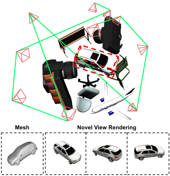
In this work, we address the problem of actively reconstructing objects of one or multiple interesting semantic classes in an initially unknown 3D environment using posed RGB-D camera measurements. Given a limited measurement budget, our goal is to obtain accurate 3D representations of the objects of interest by positioning a robotic camera online, i.e. during a mission, as shown in Fig. 1. Most existing approaches for active reconstruction [8, 20, 17, 22, 29, 31, 10, 12, 6, 27] aim at reconstructing the whole scene, without distinguishing between the observed objects. Since they do not incorporate semantics within planning pipelines, these methods cannot target specific objects of interest.
Recently, implicit neural representations [14, 24], e.g. Neural Radiance Fields (NeRFs) [15], are attracting increasing attention as a compact form for dense scene representation. Follow-up works [26, 18, 4, 16] address the inherent training inefficiency of implicit neural representations by introducing hybrid structures, which learn scene attributes using sparse feature voxel grids combined with shallow multi-layer perceptrons (MLPs). This efficient structure enables deploying implicit neural representations in online robotic tasks [35, 32, 34], while preserving their continuous representation capabilities. In this work, we exploit hybrid implicit neural representations as our map representation for semantic-targeted active implicit reconstruction.
Active implicit reconstruction is an advancing research field. State-of-the-art works adopt next-best-view planning strategies to find the most informative measurements for training implicit neural representations. While showing promising results, these methods [22, 29, 31, 10, 12, 6, 27] only focus on uniformly reconstructing global scenes. They do not account for semantic information to distinguish objects of interest and reconstruct them in an adaptive, targeted way. In the context of semantics, recent works [33, 28, 1, 25] propose integrating 2D semantic labels into implicit neural representations to enhance semantic understanding capabilities. These approaches show accurate and consistent semantic rendering at novel views via multi-view learning. However, they have not been used for active reconstruction applications. To bridge the gap between active reconstruction and semantic implicit neural representations, we propose a new framework that enables guiding view planning toward objects of interest in an unknown environment.
Our main contribution is a novel framework, STAIR, for semantic-targeted active implicit reconstruction. Given posed RGB-D measurements and corresponding 2D semantic labels, our approach utilises implicit neural representations to learn occupancy, colour, and semantic fields associated with the scene. A key component of our approach is a new utility function for next-best-view planning using semantic implicit neural representations, which enables trading off between exploring the unknown environment and exploiting information about objects of interest as they are discovered.
We make the following three claims: (i) our STAIR framework shows better performance in terms of reconstructed mesh and RGB rendering quality compared to pure exploration and heuristic baselines that do not consider semantics for view planning; (ii) our method outperforms a state-of-the-art semantic-targeted active reconstruction system using explicit map representations both in mapping and planning aspects; and (iii) our utility function for planning balances between exploration and exploitation to handle challenging scenes containing many occlusions. To support reproducibility and future research, our simulation environment and implementation will be released at: https://github.com/dmar-bonn/stair.
II Related Work
Our approach lies at the intersection of active reconstruction using semantics and implicit neural representations. In this section, we overview related work in these fields.
II-A Semantic-Targeted Active Explicit Reconstruction
Semantic understanding is crucial for many autonomous robotic tasks in unknown environments. Recent advancements in deep learning-based semantic segmentation facilitate the seamless integration of semantic understanding onboard robotic systems [7]. In the context of active reconstruction, several works propose integrating semantics into explicit maps to enable semantic-targeted view planning.
Papatheodorou et al. [23] use an occupancy voxel map to model the background for exploring unknown environments. Once objects of predefined interesting semantic classes are found, they use adaptive-resolution octree-based signed distance function mapping to reconstruct the objects in detail. Lehnert et al. [13] design a 3D camera array to obtain multiple measurements from different perspectives. The objects of interest detected in each measurement are used to calculate the gradient indicating the most likely direction of movement to observe them. Burusa et al. [2] calculate the expected information gain based on the confidence score of a voxel belonging to interesting semantic classes. Similar to our problem setup, Zaenker et al. [30] propose a semantic-targeted active explicit reconstruction system based on occupancy voxel maps and apply it to reconstruct fruits in agricultural robotics applications. To guide targeted next-best-view planning, they assign higher utility for candidate views that observe more unknown voxels close to already detected objects of interest.
Our approach shares the same idea of using semantic information to conduct view planning towards objects of interest. However, different from previous works that rely on discrete explicit maps, we exploit recent advances in implicit neural representations to improve the reconstruction quality.
II-B Active Implicit Reconstruction
Implicit neural representations are a powerful tool for 3D reconstruction due to their continuous representation capabilities. Recent work has explored how to exploit these benefits in active reconstruction settings.
Pan et al. [22] model the radiance field as Gaussian distribution and actively collect images by evaluating the reduction of uncertainty assuming new inputs at candidate views. Exploiting fast rendering of Instant-NGP [16], Sünderhauf et al. [27] train an ensemble of NeRF models for a single scene and measure uncertainty as the variance of the ensemble’s prediction, which is used to conduct next-best-view selection. Jin et al. [10] incorporate uncertainty estimation into image-based neural rendering to predict rendering uncertainty at novel views, enabling mapless next-best-view planning. Leveraging the differentiability of the implicit neural representations, Yan et al. [29] optimise next-best-view generation towards views with high uncertainty. Following a different paradigm, Pan et al. [21] utilise a view number prediction network to predict the number of views required to reconstruct a specific unknown object using NeRF, allowing for one-shot view sequence generation without online replanning.
Our work follows these lines by using implicit neural representations for active reconstruction. Different from previous methods that uniformly reconstruct a scene or an object, our approach integrates semantic understanding into an implicit neural representation to achieve semantic-targeted active implicit reconstruction.
II-C Semantics in Implicit Neural Representations
Recent works propose lifting 2D semantic information into 3D to generate a consistent semantic field by exploiting the multi-view consistency from learning implicit neural representations. Zhi et al. [33] extend vanilla NeRF to jointly encode the semantics along with the scene appearance and geometry. Their results show multi-view consistent and smooth semantic rendering at novel views, even given sparse or noisy 2D semantic labels as supervision signals. Siddiqui et al. [25] and Bhalgat et al. [1] further incorporate instance segmentation into implicit neural representations. Vora et al. [28] train a 3D network to convert a learned density field into a semantic field, which generalises across scenes.
In contrast to previous approaches for generating semantic implicit neural representations, Kelly et al. [11] use semantic information to train NeRFs in a targeted way. To reconstruct objects of interest in the scene at higher quality, they propose a denser sampling of training examples around these objects based on semantic segmentation. DietNeRF [9] proposes a semantic consistency loss to regularise rendering from arbitrary views, encouraging consistent high-level semantics. This additional loss alleviates the degenerate performance commonly observed in NeRF training with sparse views.
While semantics offer rich scene understanding capabilities in implicit neural representations, they have not yet been applied for active implicit reconstruction problems. We bridge this gap by introducing a framework for semantic-targeted active reconstruction based on implicit neural representations. Our approach is applicable for similar problems tackled by current methods using active explicit reconstruction to target objects of interest in unknown environments [30, 2, 23]. However, we exploit the advantages of underlying implicit neural representations to further improve the reconstruction quality.
III Our Approach
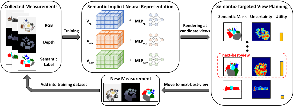
We propose STAIR, a novel framework for semantic-targeted active implicit reconstruction in autonomous robotics tasks. An overview of our framework is shown in Fig. 2. Our goal is to actively reconstruct objects of interest in an initially unknown environment using a robot equipped with a RGB-D camera. We utilise an implicit neural representation consisting of sparse feature voxel grids and MLPs as our map representation. Given collected posed RGB-D measurements and corresponding semantic labels, we incrementally train our map representation to model the occupancy probability, colour, and semantic information in continuous 3D space. To guide semantic-targeted view planning, we sample candidate views in a predefined action space and evaluate the utility of each view based on uncertainty estimates from the occupancy distribution and semantic rendering. The candidate view with the highest utility value is selected as the location for the next measurement. We iterate between training and planning until a maximum allowable number of measurements is reached.
III-A Semantic Implicit Neural Representation
Similar to DVGO [26], our map representation consists of sparse feature voxel grids and MLPs to balance representation capabilities and training efficiency. We maintain features for different modalities of the scene: spatial occupancy (occ), RGB colour (rgb), and semantics (sem), in three voxel grids , , and , respectively. For any point in space, we can query its modality feature by trilinear interpolation in the corresponding voxel grid expressed as:
| (1) |
where , is the queried modality feature vector at position , is the feature voxel grid of corresponding modality with feature channels, and , , are the spatial resolution dimensions.
The queried modality features at point are then interpreted by modality-specific MLPs into per-point occupancy probability , RGB colour , and semantic probability vector , with as the number of total semantic classes. We use a positional encoding function [15] to map position into a higher-dimensional space. Note that we do not consider view-dependent colour emission in this work.
III-B Training of Map Representation
Our map representation is updated online during a mission. Given a set of posed RGB-D measurements obtained by the robot camera and their semantic labels, we jointly train our feature voxel grids and MLPs using differentiable volume rendering [15]. To render colour, depth, and semantics for a ray cast from a measurement view, we uniformly sample points along the ray with as the depth value from the sampling point to its view origin. Following UNISURF [18], occupancy-based volume rendering for predicted colour , depth , and semantic probability observed from ray is given by:
| (2) | |||
| (3) | |||
| (4) |
with:
| (5) |
where is the weight of modality value at and is accumulated transmittance, indicating the probability of ray reaching without being blocked by built surfaces.
We supervise the training using the loss terms:
| (6) | ||||
| (7) | ||||
| (8) |
where , , and are the recorded colour, depth, and semantic label respectively of ray in the measurements, CE refers to the cross entropy loss and denotes the set of rays in the training batch. The total training loss is then:
| (9) |
with the factors balancing the weight of each term in the loss function.
We incrementally train our map representation for a constant number of iterations when a new measurement arrives. To avoid overfitting to the latest measurement, we collect our training batch for each training iteration from both previous measurements and the latest measurement. We assign the probability of sampling each training ray example as being inversely proportional to its total sampled time to ensure uniform sampling across the whole training dataset. After training, our map representation is used for semantic-targeted view planning, introduced next.
III-C Semantic-Targeted View Planning
A key aspect in our framework is a utility function that adaptively guides view planning by trading off between exploration and exploitation. We first introduce our sampling strategy for generating candidate views and then elaborate on how we calculate utility values for next-best-view selection.
To generate candidate views, we adopt a two-stage sampling strategy. We first uniformly sample candidate views on the hemispherical action space. We evaluate the individual utility at each view and select the views of top utility values. We then resample new candidate views around each of these views to obtain a fine-grained utility evaluation. Finally, the candidate view with the highest utility value is selected as the next-best-view.
Our utility quantification requires uncertainty estimates and semantic rendering. Uncertainty estimation indicates parts of the scene that are unexplored or still not well-reconstructed. On the other hand, semantic rendering provides masks to distinguish objects of interest, allowing for view selection in a targeted way. We derive the uncertainty estimates from our trained occupancy field. For a candidate view , we sample points on each of rays cast from the view. We define the uncertainty at each sampling point as its entropy:
| (10) |
where is the complementary occupancy probability. Note that we do not consider the entropy of sampling points behind the built object surface. Thus, the total entropy along a ray is:
| (11) |
where is the accumulated transmittance term introduced in Eq. 5. The total uncertainty rendered at view is:
| (12) |
which we define as our exploration (er) score. This term does not distinguish between the uncertainty values associated with different objects. Instead, it quantifies the total uncertainty at a view. To account for objects of interest based on their semantic meaning, we apply a mask to the uncertainty according to whether or not the objects are relevant for semantic-targeted active planning:
| (13) | |||
| (14) |
where is the predicted semantic probability vector obtained using Eq. 4 and is a set of identifiers for the interesting semantic classes. We denote the sum of pixelwise uncertainty from the objects of interest as our exploitation (et) score, which guides view planning towards target objects.
To trade off between exploring the unknown environment and exploiting information about objects of interest as they are discovered, we compute the utility value of a candidate view as the sum of exploitation and weighted exploration score, with as the weight factor:
| (15) |
IV Experimental Results
IV-A Experimental Setup
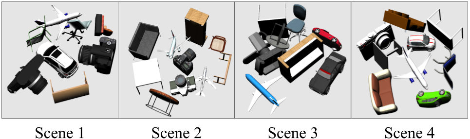
Simulator. We spawn ShapeNet [3] models of different semantic classes with random poses in Gazebo [19] to build simulation scenes. We consider semantic classes in our simulator: car, airplane, sofa, chair, table, camera, and background. Four scenes used in the planning experiments are shown in Fig. 3. All scenes consider a bounding box size of m m m. We set our camera action space as a scene-centric hemisphere with m radius and camera views targeting the scene origin. All RGB-D measurements are at px px resolution. To acquire the semantic labels, pre-trained semantic segmentation models can be applied; however, in this work, we use ground truth semantics from the simulator to focus on evaluating planning performance.
Training Setup. We use a grid size of for all three feature voxel grids. We set the feature channels as , , and . The comprises two hidden layers with 128 channels, while consists of two hidden layers with 32 channels. We simply use an identity mapping as and no positional encoding for modelling semantics since the semantic field is smooth and exists in a low-frequency domain. We set , and in Eq. 9. For each training iteration, we use a batch size of with training examples from all previous measurements and training examples from the current measurement. We train our map representation for steps before conducting view planning, which takes approximately s with our PyTorch implementation running on a single NVIDIA RTX A5000 GPU.
Planning Setup. For candidate view sampling introduced in Sec. III-C, we set , , and , giving a total of views. To render semantic and uncertainty maps at a candidate view, we use and . One planning step takes around s under this sampling and rendering configuration. The exploration weight in Eq. 15 is . We select car in Scene 1, camera in Scene 2, sofa in Scene 3, car and airplane in Scene 4 as the interesting classes for semantic-targeted active reconstruction. The maximum number of planning steps is set to for all experiments.
Evaluation Metrics. We evaluate the reconstruction results with test view rendering performance and mesh quality. We report the peak signal-to-noise ratio (PSNR) [15] as the rendering metric and use F1-score to measure overall mesh quality. Since our goal is to reconstruct objects of interest, we only consider these objects in the metrics calculations. Hence, when rendering at test views or extracting meshes from our trained map representation, we only keep objects of interest by setting the occupancy probability of points with uninteresting semantic predictions to zero.
For calculating PSNR, we render colour images at uniformly distributed test views and compare the predictions with ground truth images. We average the PSNR over all test views as the final rendering metric. For mesh quality evaluation, we first extract the mesh of objects of interest from our trained occupancy field using Multiresolution IsoSurface Extraction [14] with a threshold of . We uniformly sample points on both the extracted mesh and the ground truth mesh. The precision is calculated as the fraction of points on the extracted mesh that are closer than a threshold distance to points on the ground truth mesh. Similarly, the completeness is the fraction of points on the ground truth mesh that match points on the extracted mesh within a threshold distance. We use cm as the threshold value for precision and completeness calculations. Finally, the F1-score is the harmonic mean of precision and completeness.
IV-B Active Implicit Reconstruction
Our first experiment shows that our semantic-targeted view planning method achieves better reconstruction quality in terms of rendering performance and mesh quality compared to pure exploration and heuristic baselines that do not consider semantics. The map representations and training configurations are the same for all methods, hence the reconstruction quality differs purely as the consequence of collected measurements using different planning strategies. We consider the following planning methods:
-
•
Ours: selects the view with the highest utility value defined in Eq. 15;
-
•
Exploration: selects the view with the highest exploration score as calculated by Eq. 12;
-
•
Fixed Pattern: follows the spiral pattern view sequence to cover the hemispherical action space;
-
•
Max. View Distance: selects the view that maximises the view distance to all previously visited views;
-
•
Uniform: selects a random view from uniformly sampled candidate views.
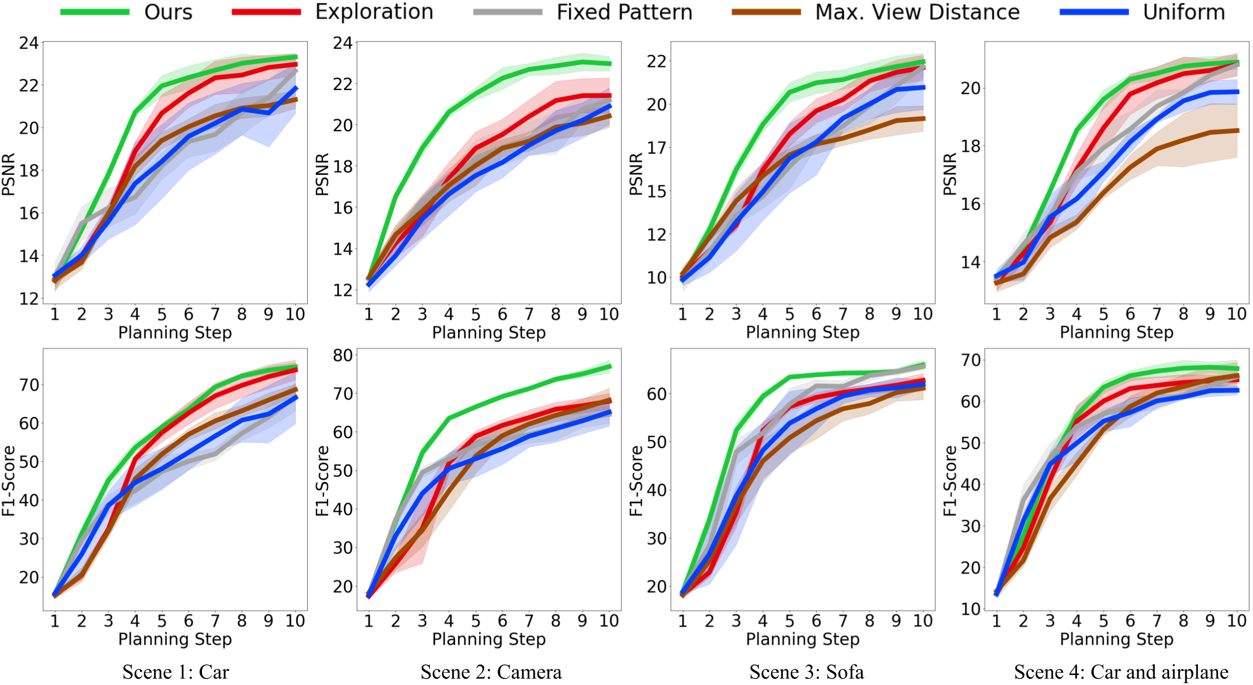
For all experiment runs, we start with a measurement from the top view and use different planning methods to select the next view to acquire a new measurement, which, together with all previous measurements, is used to train our map representation. We evaluate reconstruction performance after every planning step. For each test scene and planning method, we run trials and report the average PSNR and F1-score with standard deviations along the planning steps.
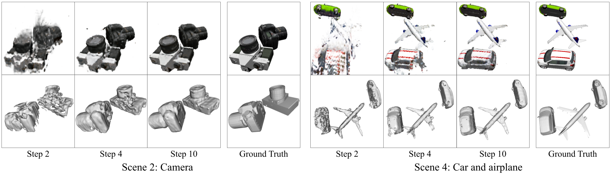
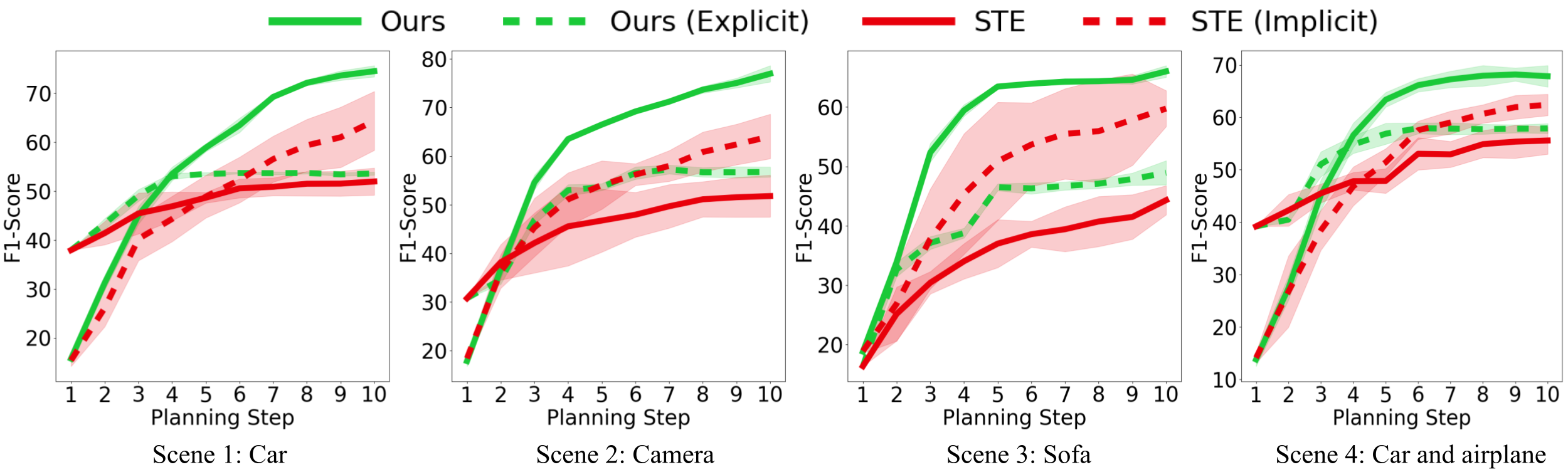
The experiment results are given in Fig. 4. Next-best-view planning guided by our approach shows steeper-rising metric curves, indicating more efficient reconstruction compared to baselines that do not consider semantic information. This verifies that our STAIR framework benefits from integrating semantics in an implicit neural representation to achieve semantic-targeted active reconstruction. Our approach has the lowest standard deviations across all scenes, indicating its robust performance. In Fig. 5, we show two examples of how novel view rendering and object meshes improve along planning steps using our approach.
IV-C Comparison Against Active Explicit Reconstruction
In this experiment, we compare our STAIR framework against semantic-targeted active explicit reconstruction to show the advantages of using an implicit neural representation for our task. Specifically, we compare against the approach of Zaenker et al. [30], which we denote as STE to indicate semantic-targeted planning based on explicit map representations. STE fuses RGB-D measurements and 2D semantic labels into an explicit semantic occupancy grid map and biases planning towards the objects of interest as they are built in the map by assigning higher utility to unknown voxels close to objects of interest. For comparability, we use the same grid size of for their map.
To further investigate the sources of performance difference between our approach and STE, we cross-validate these two active reconstruction frameworks by combining measurements collected by each framework with the other mapping system. After the online planning experiments, we fuse the measurements collected by our framework into an explicit occupancy map used in the STE approach. We denote this combination as Ours (Explicit). The result of this combination indicates whether the performance gain originates from our view planning results. Similarly, we use the measurements collected by the STE approach to train our implicit neural representation, which we denote as STE (Implicit). This combination exposes how different map representations influence the reconstruction performance.
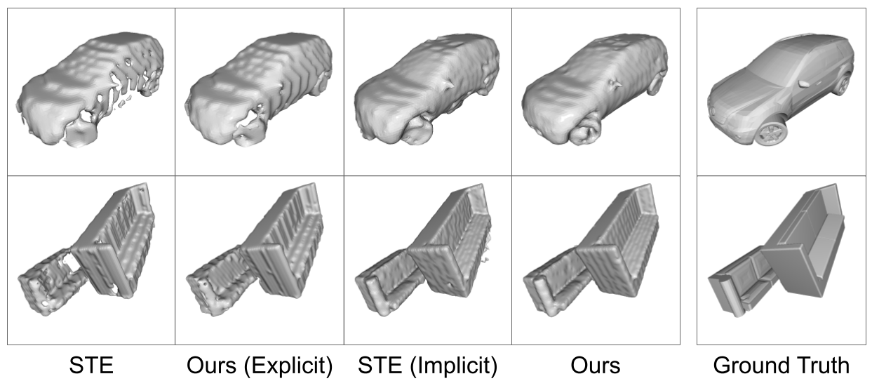
The results are shown in Fig. 6. Our framework performs better than the STE method. The performance gain can be decomposed into two aspects. First, comparing STE (Implicit) and STE suggests that, given the same measurements, our implicit neural representation improves reconstruction quality compared to explicit occupancy mapping. This justifies the choice of using implicit neural representations in our active reconstruction framework. Second, as seen by comparing Ours (Explicit) and STE, even when using explicit occupancy mapping, measurements acquired using our planning approach lead to better reconstruction quality. This indicates that our semantic-targeted view planning based on dense semantic and uncertainty rendering enables finding more informative views to reconstruct objects of interest. Fig. 7 visualises the final extracted meshes using the four methods. Meshes extracted from our implicit neural representation show complete surfaces with more high-frequency details compared to those from explicit maps.
IV-D Ablation Study
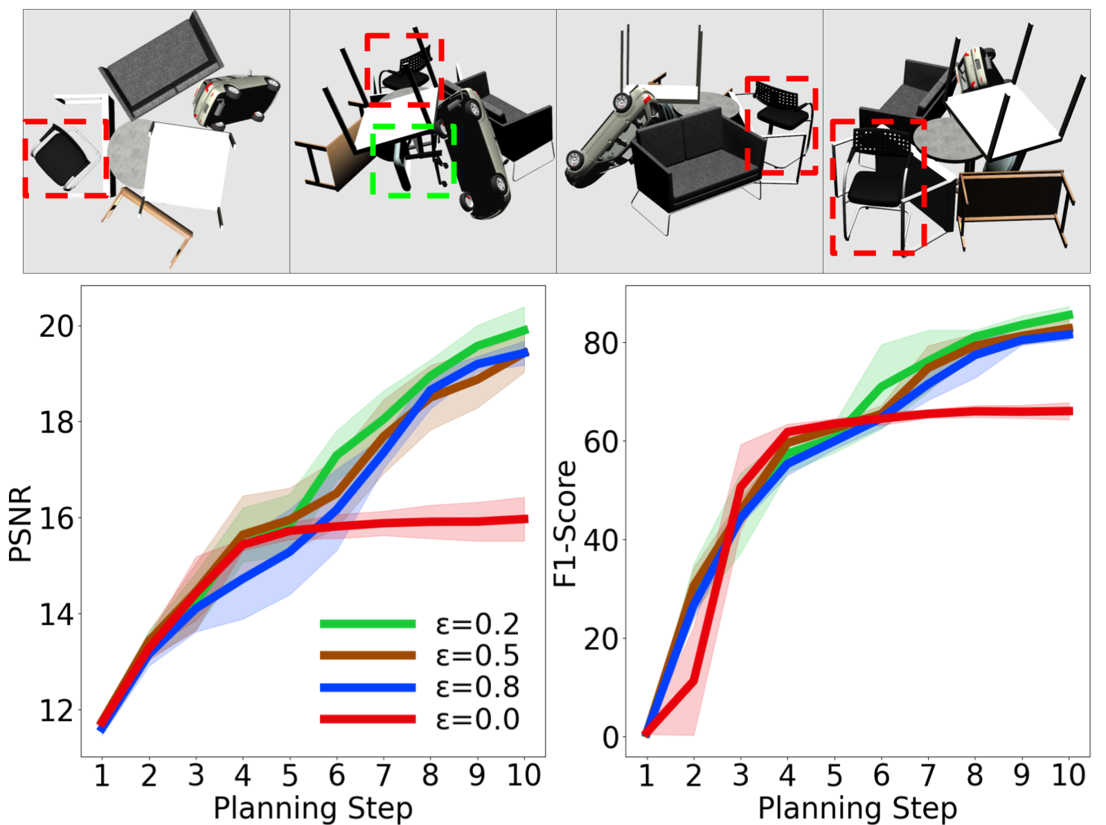
The final experiment justifies our design choice for the utility function introduced in Sec. III-C. We show that an exploration term is necessary for semantic-targeted view planning in an unknown environment. For this purpose, we design a challenging scene, as shown in Fig. 8, where two objects of interest (chairs) are separated by other objects. We start from the top view, from which only one chair is seen and the other one is occluded. We compare the planning approach using the exploitation-only score in Eq. 13, i.e. , and our proposed utility function in Eq. 15 with values of , , and to investigate the influence of varying the exploration term proportion.
Fig. 8 compares the reconstruction performance in the test scene. Semantic-targeted view planning without exploration focuses only on already detected objects of interest. As a result, this planning strategy does not explore the unknown environment to find other potential objects of interest in the scene, leading to inferior overall reconstruction performance. In contrast, our approach trades off between exploring the unknown environment and exploiting information about objects of interest as they are discovered. The results indicate that a small exploration term is sufficient to achieve such behaviour, while up-weighting exploration deteriorates semantic-targeted view planning performance.
V Conclusions
We presented STAIR, a novel framework for semantic-targeted active implicit reconstruction. Our approach exploits implicit neural representation with semantic understanding capabilities. By combining uncertainty estimation and semantic rendering, our semantic-targeted view planning strategy gathers information about objects of interest in unknown environments. Active planning experiments demonstrate the superior performance of our framework compared to implicit reconstruction baselines that do not consider semantics and a semantic-targeted approach using an explicit map representation. We also show that considering exploration is crucial for semantic-targeted view planning in challenging scenes to enable finding occluded objects of interest. One limitation of our current work is the assumption of access to accurate semantic labels. In the presence of noisy semantics, future work will consider integrating the uncertainty of semantic rendering in our planning pipeline.
References
- Bhalgat et al. [2023] Y. Bhalgat, I. Laina, J. F. Henriques, A. Zisserman, and A. Vedaldi, “Contrastive Lift: 3D Object Instance Segmentation by Slow-Fast Contrastive Fusion,” in Proc. of the Conf. on Neural Information Processing Systems, 2023.
- Burusa et al. [2023] A. K. Burusa, J. Scholten, D. R. Rincon, X. Wang, E. J. van Henten, and G. Kootstra, “Efficient Search and Detection of Relevant Plant Parts using Semantics-Aware Active Vision,” arXiv preprint arXiv:2306.09801, 2023.
- Chang et al. [2015] A. X. Chang, T. Funkhouser, L. Guibas, P. Hanrahan, Q. Huang, Z. Li, S. Savarese, M. Savva, S. Song, H. Su, J. Xiao, L. Yi, and F. Yu, “ShapeNet: An Information-Rich 3D Model Repository,” arXiv preprint arXiv:1512.03012, 2015.
- Chen et al. [2022] A. Chen, Z. Xu, A. Geiger, J. Yu, and H. Su, “TensoRF: Tensorial Radiance Fields,” in Proc. of the Europ. Conf. on Computer Vision, 2022.
- Chen et al. [2011] S. Chen, Y. Li, and N. M. Kwok, “Active Vision in Robotic Systems: A Survey of Recent Developments,” Intl. Journal of Robotics Research, vol. 30, no. 11, pp. 1343–1377, 2011.
- He et al. [2023] S. He, C. D. Hsu, D. Ong, Y. S. Shao, and P. Chaudhari, “Active Perception using Neural Radiance Fields,” arXiv preprint arXiv:2310.09892, 2023.
- Hurtado and Valada [2022] J. V. Hurtado and A. Valada, “Semantic Scene Segmentation for Robotics,” in Deep Learning for Robot Perception and Cognition. Academic Press, 2022, pp. 279–311.
- Isler et al. [2016] S. Isler, R. Sabzevari, J. Delmerico, and D. Scaramuzza, “An Information Gain Formulation for Active Volumetric 3D Reconstruction,” in Proc. of the IEEE Intl. Conf. on Robotics & Automation, 2016.
- Jain et al. [2021] A. Jain, M. Tancik, and P. Abbeel, “Putting NeRF on a Diet: Semantically Consistent Few-Shot View Synthesis,” in Proc. of the IEEE/CVF Intl. Conf. on Computer Vision, 2021.
- Jin et al. [2023] L. Jin, X. Chen, J. Rückin, and M. Popović, “NeU-NBV: Next Best View Planning Using Uncertainty Estimation in Image-Based Neural Rendering,” in Proc. of the IEEE/RSJ Intl. Conf. on Intelligent Robots and Systems, 2023.
- Kelly et al. [2023] S. Kelly, A. Riccardi, E. Marks, F. Magistri, T. Guadagnino, M. Chli, and C. Stachniss, “Target-Aware Implicit Mapping for Agricultural Crop Inspection,” in Proc. of the IEEE Intl. Conf. on Robotics & Automation, 2023.
- Lee et al. [2022] S. Lee, L. Chen, J. Wang, A. Liniger, S. Kumar, and F. Yu, “Uncertainty Guided Policy for Active Robotic 3D Reconstruction using Neural Radiance Fields,” IEEE Robotics and Automation Letters, vol. 7, no. 4, pp. 12 070–12 077, 2022.
- Lehnert et al. [2019] C. Lehnert, D. Tsai, A. Eriksson, and C. McCool, “3D Move to See: Multi-Perspective Visual Servoing for Improving Object Vews with Semantic Segmentation,” in Proc. of the IEEE/RSJ Intl. Conf. on Intelligent Robots and Systems, 2019.
- Mescheder et al. [2019] L. Mescheder, M. Oechsle, M. Niemeyer, S. Nowozin, and A. Geiger, “Occupancy Networks: Learning 3D Reconstruction in Function Space,” in Proc. of the IEEE/CVF Conf. on Computer Vision and Pattern Recognition, 2019.
- Mildenhall et al. [2020] B. Mildenhall, P. P. Srinivasan, M. Tancik, J. T. Barron, R. Ramamoorthi, and R. Ng, “NeRF: Representing Scenes as Neural Radiance Fields for View Synthesis,” in Proc. of the Europ. Conf. on Computer Vision, 2020.
- Müller et al. [2022] T. Müller, A. Evans, C. Schied, and A. Keller, “Instant Neural Graphics Primitives with a Multiresolution Hash Encoding,” ACM Trans. on Graphics, vol. 41, no. 4, pp. 102:1–102:15, 2022.
- Naazare et al. [2022] M. Naazare, F. G. Rosas, and D. Schulz, “Online Next-Best-View Planner for 3D-Exploration and Inspection with a Mobile Manipulator Robot,” IEEE Robotics and Automation Letters, vol. 7, no. 2, pp. 3779–3786, 2022.
- Oechsle et al. [2021] M. Oechsle, S. Peng, and A. Geiger, “UNISURF: Unifying Neural Implicit Surfaces and Radiance Fields for Multi-View Reconstruction,” in Proc. of the IEEE/CVF Intl. Conf. on Computer Vision, 2021.
- [19] Open Robotics, “Gazebo.” [Online]. Available: https://gazebosim.org
- Palazzolo and Stachniss [2018] E. Palazzolo and C. Stachniss, “Effective Exploration for MAVs Based on the Expected Information Gain,” Drones, vol. 2, no. 1, pp. 59–66, 2018.
- Pan et al. [2024] S. Pan, L. Jin, H. Hu, M. Popović, and M. Bennewitz, “How Many Views Are Needed to Reconstruct an Unknown Object Using NeRF?” in Proc. of the IEEE Intl. Conf. on Robotics & Automation, 2024.
- Pan et al. [2022] X. Pan, Z. Lai, S. Song, and G. Huang, “ActiveNeRF: Learning Where to See with Uncertainty Estimation,” in Proc. of the Europ. Conf. on Computer Vision, 2022.
- Papatheodorou et al. [2023] S. Papatheodorou, N. Funk, D. Tzoumanikas, C. Choi, B. Xu, and S. Leutenegger, “Finding Things in the Unknown: Semantic Object-Centric Exploration with an MAV,” in Proc. of the IEEE Intl. Conf. on Robotics & Automation, 2023.
- Park et al. [2019] J. J. Park, P. Florence, J. Straub, R. Newcombe, and S. Lovegrove, “DeepSDF: Learning Continuous Signed Distance Functions for Shape Representation,” in Proc. of the IEEE/CVF Conf. on Computer Vision and Pattern Recognition, 2019.
- Siddiqui et al. [2023] Y. Siddiqui, L. Porzi, S. R. Bulò, N. Müller, M. Nießner, A. Dai, and P. Kontschieder, “Panoptic Lifting for 3D Scene Understanding with Neural Fields,” in Proc. of the IEEE/CVF Conf. on Computer Vision and Pattern Recognition, 2023.
- Sun et al. [2022] C. Sun, M. Sun, and H. Chen, “Direct Voxel Grid Optimization: Super-fast Convergence for Radiance Fields Reconstruction,” in Proc. of the IEEE/CVF Conf. on Computer Vision and Pattern Recognition, 2022.
- Sünderhauf et al. [2023] N. Sünderhauf, J. Abou-Chakra, and D. Miller, “Density-aware NeRF Ensembles: Quantifying Predictive Uncertainty in Neural Radiance Fields,” in Proc. of the IEEE Intl. Conf. on Robotics & Automation, 2023.
- Vora et al. [2022] S. Vora, N. Radwan, K. Greff, H. Meyer, K. Genova, M. S. M. Sajjadi, E. Pot, A. Tagliasacchi, and D. Duckworth, “NeSF: Neural Semantic Fields for Generalizable Semantic Segmentation of 3D Scenes,” IEEE Trans. on Machine Learning Research, 2022.
- Yan et al. [2023] D. Yan, J. Liu, F. Quan, H. Chen, and M. Fu, “Active Implicit Object Reconstruction Using Uncertainty-Guided Next-Best-View Optimization,” IEEE Robotics and Automation Letters, vol. 8, no. 10, pp. 6395–6402, 2023.
- Zaenker et al. [2021] T. Zaenker, C. Smitt, C. McCool, and M. Bennewitz, “Viewpoint Planning for Fruit Size and Position Estimation,” in Proc. of the IEEE/RSJ Intl. Conf. on Intelligent Robots and Systems, 2021.
- Zhan et al. [2022] H. Zhan, J. Zheng, Y. Xu, I. Reid, and H. Rezatofighi, “ActiveRMAP: Radiance Field for Active Mapping And Planning,” arXiv preprint arXiv:2211.12656, 2022.
- Zhang et al. [2023] X. Zhang, D. Wang, S. Han, W. Li, B. Zhao, Z. Wang, X. Duan, C. Fang, X. Li, and J. He, “Affordance-Driven Next-Best-View Planning for Robotic Grasping,” in Proc. of the Conf. on Robot Learning, 2023.
- Zhi et al. [2021] S. Zhi, T. Laidlow, S. Leutenegger, and A. J. Davison, “In-Place Scene Labelling and Understanding with Implicit Scene Representation,” in Proc. of the IEEE/CVF Intl. Conf. on Computer Vision, 2021.
- Zhong et al. [2023] X. Zhong, Y. Pan, J. Behley, and C. Stachniss, “SHINE-Mapping: Large-Scale 3D Mapping Using Sparse Hierarchical Implicit Neural Representations,” in Proc. of the IEEE Intl. Conf. on Robotics & Automation, 2023.
- Zhu et al. [2022] Z. Zhu, S. Peng, V. Larsson, W. Xu, H. Bao, Z. Cui, M. R. Oswald, and M. Pollefeys, “NICE-SLAM: Neural Implicit Scalable Encoding for SLAM,” in Proc. of the IEEE/CVF Conf. on Computer Vision and Pattern Recognition, 2022.