Reduced model and nonlinear analysis of localized instabilities of residually stressed cylinders under axial stretch

Abstract

In this paper we present a dimensional reduction to obtain a one-dimensional model to analyze localized necking or bulging in a residually stressed circular cylindrical solid. The nonlinear theory of elasticity is first specialized to obtain the equations governing the homogeneous deformation. Then, to analyze the non-homogeneous part, we include higher order correction terms of the axisymmetric displacement components leading to a three-dimensional form of the total potential energy functional. Details of the reduction to the one-dimensional form are given. We focus on a residually stressed Gent material and use numerical methods to solve the governing equations. Two loading conditions are considered. In the first, the residual stress is maintained constant, while the axial stretch is used as the loading parameter. In the second, we keep the pre-stretch constant and monotonically increase the residual stress until bifurcation occurs. We specify initial conditions, find the critical values for localized bifurcation and compute the change in radius during localized necking or bulging growth. Finally, we optimize material properties and use the one-dimensional model to simulate necking or bulging until the Maxwell values of stretch are reached.

1 Introduction

In 1890, Mallock Mallock (1890) described the sequence of events leading up to localized bulging of thin-walled India-rubber (natural rubber) tubes subject to internal fluid pressure. In particular, he observed that the tube maintains its cylindrical form until the increase in radius remains proportional to the reference radius. But, when more fluid is introduced the tube becomes unstable and the internal pressure diminishes.

When more fluid is introduced then necessary to expand to its stable limit, the tube no longer remains cylindrical throughout its length, but assumes the form of a cylinder with one or more bulges. He observed that the diameter of the part which remains cylindrical, though greater than the reference diameter, is less than that attained at the stable limit. This is the first documented experiment in which bulging is induced by internal pressure in thin-walled rubber tubes, but it is only in recent years that it has been recognized that such nonlinear phenomena could be used in industrial applications.

Ogden Ogden (1997) develops the theory of incremental deformation superimposed on a known finitely deformed configuration. Linear approximations in terms of the incremental deformation and its gradient are used to examine incremental constitutive laws and equilibrium equations. In the theory presented in this paper, the incremental displacement components contain higher order correction terms, allowing for a nonlinear stability analysis and for the evolution of localized necking or bulging in prismatic solids. A summary of the developments of nonlinear stability analysis of thick hyperelastic plates is given in Fu and Ogden (1999). First, the linear theory is used for two representative problems to determine the critical values for stability. The linear theory can determine the buckling mode, but not its amplitude, which can only be obtained from a fully nonlinear analysis. On the other hand, the weakly nonlinear analysis is concerned with the mode amplitude when the applied load deviates from its critical value by a small amount with the amplitude depending on a far distance variable.

Methods of nonlinear stability analysis of elastic bodies are summarized in Fu (2001). Particular attention is on using the perturbation approach to the stability analysis of elastic bodies subject to large deformation. Two types of buckling modes are considered, the first consists of stability studies in which buckling modes are periodic, the second focuses on bifurcations where the critical mode number is set to zero.

The membrane assumption is used in Fu et al. (2008) to analyze the bifurcation conditions of an infinitely long hyperelastic tube with the axial stretch maintained uniform at infinity, while inflated by internal pressure. The bifurcation conditions and the near-critical behavior are determined analytically. It is shown that the bifurcation mode having zero wave number correctly describes localized bulging and necking initiation, which grow and evolve into a two-phase deformation. The near-critical post-bifurcation analysis is used to derive the amplitude equation, which is used to determine under what conditions a localized solution is possible. A more realistic case of an inflated tube with closed ends is considered in Pearce and Fu (2010). There, the entire bulging or necking process is determined, from initiation to the fully nonlinear propagation and the stability properties of the weakly nonlinear and fully nonlinear solutions are evaluated.

The use of the membrane theory to assess localized bulging in cylindrical tubes with finite wall thickness may not lead to accurate results. This is addressed in Fu et al. (2016), where the theory of nonlinear elasticity is used to derive an explicit bifurcation condition for localized bulging in a hyperelastic tube of arbitrary thickness subjected to internal pressure and axial extension. The condition requires that the Jacobian determinant of the internal pressure and resultant axial force, each considered a function of the two principal stretches, vanishes. Further insight into the bifurcation condition derived in Fu et al. (2016) is given in Yu and Fu (2022), where it is applied to derive the localized condition of an inflated hyperelastic tube and to the axisymmetric necking of a thin sheet subject to equibiaxial stretching Fu et al. (2018).

For thin-walled tubes the conservation laws reduce to ordinary differential equation and when the membrane assumption is no longer applicable, these become nonlinear partial differential equations. Even the weakly nonlinear near-critical analysis is no longer trivial, but can be performed using asymptotic methods, while the fully nonlinear post-buckling behavior relies on finite element techniques Ye et al. (2020).

Experimental data are used in Wang et al. (2019) to validate the theoretical prediction of the initiation and propagation pressures in rubber tubes with different lengths, wall thicknesses and end conditions. It is found that for constant axial force the initiation pressure is given by a bifurcation condition and the propagation pressure is determined by Maxwell’s equal-area rule. The initiation pressure for the fixed-ends case, where the length of the tube is fixed once the pre-stretch has been applied, is again determined by a bifurcation condition, but the propagation pressure is no longer determined by Maxwell’s equal-area rule. The pressure, following bulge initiation decreases to a minimum and then rises again, the latter accompanied by bulge propagation. The experimental results of the inflated tube with fixed ends are also used in Guo et al. (2022) to validate an analytical model.

In Audoly and Hutchinson (2016) a dimensional reduction is proposed to obtain a one-dimensional energy function, which is used to analyze the fully nonlinear evolution of tensile necking in prismatic solids having an arbitrary cross-section. This is made possible by incorporating the dependence on the axial stretch and its gradient that arise during necking. In Lestringant and Audoly (2018) the method is specialized to obtain a one-dimensional diffuse interface model, which is then used to analyze localized bifurcation in nonlinear axisymmetric membrane tubes. A systematic expansion of the membrane energy in terms of the aspect ration $\varepsilon=R/L\leqslant 1$ is obtained, where $R$ and $L$ are the initial radius and length, respectively. In Audoly and Hutchinson (2019) the formulation is generalized and then applied to analyze necking of rate dependent axially stretched round bars and to necking in thin sheet materials. A systematic dimensional reduction is proposed in Lestringant and Audoly (2020a) resulting in a nonlinear structural model of prismatic solids, which again captures the strain gradient effect. The one-dimensional model allows for large and inhomogeneous changes in the shape of the cross-section and can be used to analyze localization in slender structures. In Lestringant and Audoly (2020) the one-dimensional strain gradient model is used to predict necking in cylindrical nonlinear elastic solids generated by an increase of the surface tension. The dimensional reduction methodology is adopted in Yu and Fu (2023) to obtain a one-dimensional model for the analysis of bulging or necking in an inflated hyperelastic tube with arbitrary wall thickness. The theory is applied in two limiting cases, one investigates bulging in a membrane tube, the other necking in a stretched solid cylinder. It is shown that the one-dimensional model is capable to describe the entire bulging evolution accurately as demonstrated by comparing analytical results with finite element simulations.

In this paper we derive a one-dimensional model to analyze localized necking or bulging in a residually stressed circular cylindrical solid. This study builds upon our results in Liu and Dorfmann (2023), where we investigated localized necking or bulging in a residually stressed solid cylinder with circular cross-sectional area subject to axial stretch. We used the theory of linearized incremental deformations and presented the governing equations and boundary conditions in Stroh form. The results show that following bifurcation, bulged and necked regions connected by transition zones propagate along the axial direction of the cylinder.

The paper is organized as follows. In Section 2 we formulate the three-dimensional problem and provide an explicit expression of the axial force to maintain the cylindrical form of a residually stressed solid. In Section 3 we use a dimensional reduction to obtain a one-dimensional model for the nonlinear analysis of necking and bulging. A key assumption of the theory is that the bifurcation mode varies slowly in the axial direction. The axisymmetric incremental deformation components are expanded to include higher-order correction terms. A dimensional reduction is then used to derive a one-dimensional energy functional. Minimization of the energy with respect to the stretch $\lambda$ results in a second order nonlinear differential equation. To obtain numerical results we define in Section 4 an incompressible Gent material and the explicit forms of the residual stress components. The dependence of the critical stretch and residual stress values on the material extensibility is shown. The focus in Section 5 is on the use of the one-dimensional model to simulate initiation and growth of a local bifurcation. Two loading sequences are considered. In Section 5.1 the residual stress is maintained constant and the axial stretch is used as the loading parameter. In Section 5.2 the constant pre-stretch is applied first and the residual stress is then increased monotonically until bifurcation occurs. Concluding remarks are given in Section 6.

2 Three-dimensional formulation and primary deformation

A linear bifurcation analysis was used in Liu and Dorfmann (2023) to investigate localized necking and bulging in a residually stressed solid cylinder with circular cross-sectional area subject to axial stretch. The method was based on the theory of linearized incremental deformations superimposed on a known finitely deformed configuration with the governing equations and boundary conditions given in Stroh form. Following bifurcation, bulged and necked regions develop connected by transition zones, which simply propagate along the axial direction of the cylinder. In the current paper we use a dimensional reduction to obtain a one-dimensional model for the analysis of bulging or necking in a stretched residually stressed cylindrical solid. The derived model is used to investigate the post-bifurcation behavior in the fully nonlinear regime.

We consider the application of the one-dimensional theory to investigate bifurcation of a circular cylindrical solid with reference geometry defined in cylindrical polar coordinates $(\Theta,Z,R)$ by

$$0\leqslant\Theta\leqslant 2\pi,\quad-L\leqslant Z\leqslant L,\quad 0\leqslant R\leqslant A,$$ (1)

where $A$ is the outer radius and $2L$ the initial total length, see Figure 1(a). The axial extension of the cylinder is achieved by the application of an axial force $N$ resulting in a homogeneous or inhomogeneous axisymmetric deformation. If the deformation is homogeneous, the current geometry is given by

$$0\leqslant\theta\leqslant 2\pi,\quad-l\leqslant z\leqslant l,\quad 0\leqslant r\leqslant a,$$ (2)

where $(\theta,z,r)$ are the deformed cylindrical polar coordinates, and $a$ and $2l$ are the outer radius and total deformed length, respectively. We use the standard basis vectors $(\mathbf{e}_{\theta},\mathbf{e}_{z},\mathbf{e}_{r})$ associated with both $(\Theta,Z,R)$ and $(\theta,z,r)$.

We focus attention to an incompressible material and describe a general axisymmetric deformation in the form

$$\theta=\Theta,\quad z=z(Z,R),\quad r=r(Z,R),$$ (3)

which encompasses the homogeneous and inhomogeneous cases. The corresponding deformation gradient $\mathbf{F}$ has the form

$$\mathbf{F}=\frac{r}{R}\mathbf{e}_{\theta}\otimes\mathbf{e}_{\theta}+z_{Z}\mathbf{e}_{z}\otimes\mathbf{e}_{z}+z_{R}\mathbf{e}_{z}\otimes\mathbf{e}_{r}+r_{Z}\mathbf{e}_{r}\otimes\mathbf{e}_{z}+r_{R}\mathbf{e}_{r}\otimes\mathbf{e}_{r},$$ (4)

where the subscripts $Z,R$ without a preceding comma indicate the corresponding partial derivatives. The incompressibility constraint requires that

$$\det\mathbf{F}=1.$$ (5)

It then follows from (4) that

$$z_{Z}r_{R}-z_{R}r_{Z}=0.$$ (6)

There are no mechanical forces applied to the curved surface. Therefore, in the reference configuration the residual stress $\bm{\tau}$ satisfies the traction-free boundary condition

$$\bm{\tau}\mathbf{N}=\bm{0}\quad\mathrm{on}\quad R=A,$$ (7)

where $\mathbf{N}$ denotes the outward pointing unit vector normal to the surface $R=A$. With no intrinsic couple stresses, the components of the stress $\bm{\tau}$ must satisfy the equilibrium equation

$$\mbox{Div\hskip 1.0pt}\bm{\tau}=\bm{0},$$ (8)

where Div  is the divergence operator defined in the reference configuration.

Consider a hyperelastic and incompressible material, where the mechanical properties are specified in terms of an energy function $W$ defined per unit reference volume. We follow the theory in Liu and Dorfmann (2023) and consider an energy density, which is a function of the deformation gradient $\mathbf{F}$ and of the residual stress $\bm{\tau}$ and takes the form $W(\mathbf{F},\bm{\tau})$. Rajagopal and Wineman Rajagopal and Wineman (2024) show that a body with initial stresses/pre-stresses/residual stresses cannot be isotropic in such a configuration in which it is pre-stressed. Reference is made to Hoger (1993), where a general constitutive theory is developed, which is appropriate for hyperelastic, residually stressed, transversely isotropic material subject to large deformation.

The effect of the residual stress on the constitutive function is analogous to that of a structure tensor associated with preferred directions in fiber-reinforced materials, see Holzapfel and Ogden (2010), for example. Therefore, the residually stressed material is inhomogeneous and the mechanical properties anisotropic. For the considered circular cylindrical solid we assume that the only nonzero components of $\bm{\tau}$ are $\tau_{\Theta\Theta}$ and $\tau_{RR}$ such that

$$\bm{\tau}=\tau_{\Theta\Theta}\mathbf{e}_{\theta}\otimes\mathbf{e}_{\theta}+\tau_{RR}\mathbf{e}_{r}\otimes\mathbf{e}_{r},$$ (9)

which must satisfy the zero traction boundary condition (7) and the equilibrium equation (8). The preferred direction generated by (9) coincides with the axial direction of the cylinder and the material is therefore isotropic in the plane perpendicular to this direction. Transverse isotropy is the simplest material symmetry that a material can possess and still support a residual stress, see Hoger (1985, 1993) for details.

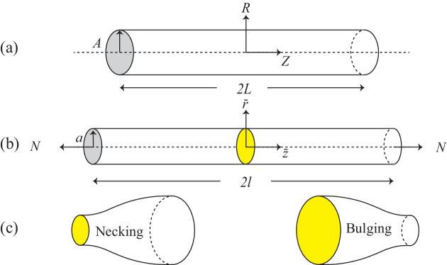
Figure 1: (a) A hyperelastic cylindrical solid with referential radius $A$, length $2L$ and zero traction on the curved surface; (b) The axial force $N$ first generates a homogeneous deformation with uniform stretch; (c) With increasing deformation, depending on the specific loading scenario, localized necking or bulging may occur, see (Liu and Dorfmann, 2023).

2.1 Homogeneous solution

In Figure 1(b) the magnitude of the applied force $N$ is below a critical value resulting in a uniform axial stretch and a radial deformation. It follows that the deformation (3) specializes to

$$\bar{\theta}=\Theta,\quad\bar{z}=\lambda Z,\quad\bar{r}=\lambda^{-1/2}R,$$ (10)

where $\lambda=l/L$ is the constant axial stretch and the superposed bar indicates quantities associated with the homogeneous solution. The deformation gradient related to (10) is then obtained as

$$\bar{\mathbf{F}}=\lambda^{-1/2}\mathbf{e}_{\theta}\otimes\mathbf{e}_{\theta}+\lambda\mathbf{e}_{z}\otimes\mathbf{e}_{z}+\lambda^{-1/2}\mathbf{e}_{r}\otimes\mathbf{e}_{r},$$ (11)

resulting in the three principal stretches

$$\lambda_{1}=\lambda^{-1/2},\quad\lambda_{2}=\lambda,\quad\lambda_{3}=\lambda^{-1/2},$$ (12)

where the subscripts 1, 2, 3 are used to indicate the $\theta$-, $z$-, $r$-directions, respectively. An increase in the axial force $N$ above a critical value will generate a bifurcation from the homogeneous cylindrical solution resulting in localized instabilities, see Figure 1(c).

We now restrict attention to a model where the residual stress components $\tau_{\Theta\Theta}$ and $\tau_{RR}$ are functions of $R$ only. Because there are only three principal stretches in $\bar{\mathbf{F}}$ it is convenient to write the energy function $W$ in the reduced form as a function of $\lambda_{1},\lambda_{2},\lambda_{3}$ and $R$ given by

$$W(\bar{\mathbf{F}},\bm{\tau})=\phi(\lambda_{1},\lambda_{2},\lambda_{3},R),$$ (13)

with (12) on the right hand side. Then, the nonzero components of the nominal stress tensor $\bar{\mathbf{T}}$ are calculated by

$$\bar{T}_{ii}=\phi_{i}-\lambda_{i}^{-1}\bar{p},\quad\mathrm{no~{}summation},$$ (14)

where $\phi_{i}=\partial\phi/\partial\lambda_{i},i=1,2,3$ and $\bar{p}$ is a Lagrange multiplier enforcing the incompressibility condition (5). For an overview of the main constituents of the nonlinear theory of residually stressed materials the interested reader is referred to Liu and Dorfmann (2023); Melnikov et al. (2021, 2022).

For the circular cylindrical geometry with uniform axial stretch the equilibrium equation $\mbox{Div\hskip 1.0pt}\bar{\mathbf{T}}=\mathbf{0}$ reduces to the single component in the radial direction

$$\frac{\mathrm{d}\bar{T}_{33}}{\mathrm{d}R}+\frac{\bar{T}_{33}-\bar{T}_{11}}{R}=0,$$ (15)

and the zero traction on the curved surface $R=0$ gives rise to

$$\bar{T}_{33}=\int_{A}^{R}\frac{\phi_{1}-\phi_{3}}{t}\mathrm{d}t.$$ (16)

The boundary conditions are used to determine the value of the Lagrange multiplier $\bar{p}$ in (14), but we omit the details for brevity.

The equilibrium condition in the axial direction requires that

$$N=2\pi\int_{0}^{A}\bar{T}_{22}R\mathrm{d}R,$$ (17)

and using (14), (15) that (17) this results in

$$N=\pi\int_{0}^{A}\left(2\phi_{2}-\lambda^{-3/2}\phi_{1}-\lambda^{-3/2}\phi_{3}\right)R\mathrm{d}R.$$ (18)

3 Derivation of a one-dimensional strain-gradient model

In this section, we perform a proper dimensional reduction to derive a one-dimensional model for the deformation and bifurcation of a residually stressed hyperelastic and incompressible cylinder. A key ingredient of the dimensional reduction methodology in Audoly and Hutchinson (2016) is the fundamental assumption that the bifurcation mode varies slowly in the axial direction, which we assume to be the case for localized necking and bulging. Therefore, in deriving the one-dimensional model, it is convenient to introduce a variable $S$ defined by

$$S=\varepsilon Z,$$ (19)

where $\varepsilon$ is a small parameter, which in our case is taken as the radius to length ratio $A/L$. The reason we introduce the variable $S$ is to identify terms of different order $\varepsilon$ in the following derivation.

We begin the analysis by defining the total potential energy $\mathcal{E}$ of a residually stressed, axisymmetrically deformed hyperelastic cylinder subject to a constant axial force $N$ by

$$\mathcal{E}=2\pi\int_{-L}^{L}\int_{0}^{A}\left(W(\mathbf{F},\bm{\tau})-\hat{N}z_{Z}\right)R\mathrm{d}R\mathrm{d}Z,$$ (20)

where the force density $\hat{N}=N/(\pi A^{2})$. In the following the stretch $\lambda$ is no longer uniform and is taken as a function of the variable $S$. Following Yu and Fu (2023) we augment the axisymmetric displacement components (3) to include the higher-order correction terms $\tilde{w},\tilde{u}$ and look for an asymptotic solution of the form

$$z(Z,R) = \dfrac{1}{\varepsilon}\int_{0}^{S}\lambda(\hat{S})\mathrm{d}\hat{S}+\varepsilon\tilde{w}(S,R)+\mathcal{O}(\varepsilon^{3}),$$ (21)

$$r(Z,R) = \lambda(S)^{-1/2}R+\varepsilon^{2}\tilde{u}(S,R)+\mathcal{O}(\varepsilon^{4}),$$ (22)

where the stretch $\lambda(S)$ can be used for the homogeneous as well as for the bifurcated solution. The updated form of the deformation gradient (11) is then given by

$$\bar{\mathbf{F}}=\lambda(S)^{-1/2}\mathbf{e}_{\theta}\otimes\mathbf{e}_{\theta}+\lambda(S)\mathbf{e}_{z}\otimes\mathbf{e}_{z}+\lambda(S)^{-1/2}\mathbf{e}_{r}\otimes\mathbf{e}_{r}.$$ (23)

Using the expansions (21) and (22) in the general form of the deformation gradient (4) gives

$$\mathbf{F}=\left[\begin{array}[]{ccc}\lambda(S)^{-1/2}+\dfrac{\tilde{u}}{R}\varepsilon^{2}&0&0\\ 0&\lambda(S)+\varepsilon^{2}\tilde{w}_{S}&\varepsilon\tilde{w}_{R}\\ 0&-\dfrac{1}{2}\varepsilon\lambda^{-3/2}\lambda^{\prime}(S)R&\lambda(S)^{-1/2}+\varepsilon^{2}\tilde{u}_{R}\end{array}\right],$$ (24)

where terms of $\mathcal{O}(\varepsilon^{3})$ and higher have been neglected. The subscripts $S,R$ without a preceding comma indicate the corresponding partial derivatives, while differentiation of $\lambda(S)$ is indicated by $\lambda^{\prime}(S)=\mathrm{d}\lambda(S)/\mathrm{d}S$. Using (19) results in the deformation gradient $\mathbf{F}$ being a function of the parameter $\varepsilon$.

The next step in deriving the one-dimensional model is to expand the energy density function $W(\mathbf{F},\mathbf{\tau})$ in terms of $\varepsilon$. This has the form

$$W(\mathbf{F},\mathbf{\tau})=W(\bar{\mathbf{F}},\mathbf{\tau})+\mathbf{\Gamma}:(\mathbf{F}-\bar{\mathbf{F}})+\frac{1}{2}(\mathbf{F}-\bar{\mathbf{F}}):\bm{\mathcal{A}}:(\mathbf{F}-\bar{\mathbf{F}})+\mathcal{O}(\varepsilon^{3}),$$ (25)

where $\mathbf{\Gamma}$ and $\bm{\mathcal{A}}$ are defined by

$$\Gamma_{\alpha i}=\frac{\partial W}{\partial F_{i\alpha}}{\Bigg{|}_{\mathbf{F}=\bar{\mathbf{F}}}},\quad\mathcal{A}_{\alpha i\beta j}=\frac{\partial^{2}W}{\partial F_{i\alpha}F_{j\beta}}{\Bigg{|}_{\mathbf{F}=\bar{\mathbf{F}}}},$$ (26)

and for the double contraction we use the convention $\mathbf{\Gamma}:(\mathbf{F}-\bar{\mathbf{F}})=\Gamma_{\alpha i}(F_{i\alpha}-\bar{F}_{i\alpha})$. The component form of (25) is then given by

$$W(\mathbf{F},\mathbf{\tau})=W(\bar{\mathbf{F}},\mathbf{\tau})+\Gamma_{\alpha i}(F_{i\alpha}-\bar{F}_{i\alpha})+\frac{1}{2}\mathcal{A}_{\alpha i\beta j}(F_{i\alpha}-\bar{F}_{i\alpha})(F_{j\beta}-\bar{F}_{j\beta})+\mathcal{O}(\varepsilon^{3}),$$ (27)

with the major symmetries $\mathcal{A}_{\alpha i\beta j}=\mathcal{A}_{\beta j\alpha i}$ satisfied. It can be shown that the residual stress tensor $\bm{\tau}$ is independent of $\varepsilon$, but we do not provide the details here.

The function $\bm{\Gamma}$ is evaluated in the homogeneous state and it is therefore convenient to use the energy function (13) defined in terms of the principal stretches (12) and we write

$$\mathbf{\Gamma}=\phi_{1}\mathbf{e}_{\theta}\otimes\mathbf{e}_{\theta}+\phi_{2}\mathbf{e}_{z}\otimes\mathbf{e}_{z}+\phi_{3}\mathbf{e}_{r}\otimes\mathbf{e}_{r}.$$ (28)

The reason we introduced the variable $S$ was to identify all terms of $\mathcal{O}(\varepsilon^{2})$ in (4). We now return to the original definition $\lambda=\lambda(Z)$ and for clarity of presentation use the shorthand notations $u=\varepsilon^{2}\tilde{u},w=\varepsilon\tilde{w}$. The energy functional (20) can then be written in the simplified form

$$\mathcal{E}=2\pi\int_{-L}^{L}\left[G(\lambda)+\mathcal{E}_{2}\right]\mathrm{d}Z,$$ (29)

where

$$G(\lambda) = \int_{0}^{A}\phi\,R\mathrm{d}R-\frac{1}{2}A^{2}\lambda\hat{N},$$

$$\mathcal{E}_{2} = \int_{0}^{A}\bigg{[}\phi_{1}\frac{u}{R}+(\phi_{2}-\hat{N})w_{Z}+\phi_{3}u_{R}$$ (30)

$$+ \frac{1}{2}\left(\mathcal{A}_{2323}w_{R}^{2}-\mathcal{A}_{2332}\lambda^{\prime}\lambda^{-3/2}Rw_{R}+\frac{1}{4}\mathcal{A}_{3232}\lambda^{\prime 2}\lambda^{-3}R^{2}\right)\bigg{]}R\mathrm{d}R,$$

where here and in what follows $\lambda^{\prime}=\mathrm{d}\lambda(Z)/\mathrm{d}Z$. Next, we calculate the incompressibility constraint (5) up to $\mathcal{O}(\varepsilon^{2})$ and obtain

$$2\lambda^{5/2}(Ru)_{R}+R(2\lambda w_{Z}+R\lambda^{\prime}w_{R})=0,$$ (31)

which allows to eliminate the variable $u$ in $\eqref{Components}_{2}$. We use the connection

$$\int_{0}^{A}\left(\phi_{1}u+\phi_{3}Ru_{R}\right)\mathrm{d}R = \int_{0}^{A}\left[\bar{T}_{11}u+\bar{T}_{33}Ru_{R}+\bar{p}\lambda^{1/2}\left(u+Ru_{R}\right)\right]\mathrm{d}R$$ (32)

$$= \bar{T}_{33}Ru\Big{|}_{0}^{A}+\int_{0}^{A}\left(\bar{p}\lambda^{1/2}(Ru)_{R}\right)\mathrm{d}R$$

$$= -\int_{0}^{A}\bar{p}\left(\frac{w_{Z}}{\lambda}+\frac{R\lambda^{\prime}w_{R}}{2\lambda^{2}}\right)R\mathrm{d}R,$$

to express $\eqref{Components}_{2}$ in the form

$$\mathcal{E}_{2} = \int_{0}^{A}\left[-\bar{p}\left(\frac{w_{Z}}{\lambda}+\frac{R\lambda^{\prime}w_{R}}{2\lambda^{2}}\right)R+R(\phi_{2}-\hat{N})w_{Z}\right.$$ (33)

$$+ \left.\frac{1}{2}R\left(\mathcal{A}_{2323}w_{R}^{2}-\mathcal{A}_{2332}\lambda^{\prime}\lambda^{-3/2}Rw_{R}+\frac{1}{4}\mathcal{A}_{3232}\lambda^{\prime 2}\lambda^{-3}R^{2}\right)\right]\mathrm{d}R.$$

In the formulation (33), the term containing the variable $w_{Z}$ can be eliminated by integration by parts and by using the definition $\bar{T}_{22}=\phi_{2}-\lambda^{-1}\bar{p}$. This allows to write the energy functional (29) in the alternative form

$$\mathcal{E}=2\pi\int_{-L}^{L}\left[G(\lambda)+\int_{0}^{A}\mathcal{M}(R,w,w_{R})\mathrm{d}R\right]\mathrm{d}Z+\left[\int_{0}^{A}2\pi R\left(\bar{T}_{22}-\hat{N}\right)w\mathrm{d}R\right]\Bigg{|}_{Z=-L}^{Z=L},$$ (34)

where

$$\mathcal{M}(R,w,w_{R})=\frac{1}{2}R\mathcal{A}_{2323}w_{R}^{2}-\frac{1}{2}R^{2}\lambda^{\prime}\left(\mathcal{A}_{2332}\lambda^{-3/2}+\bar{p}\lambda^{-2}\right)w_{R}-\bar{T}_{22,\lambda}\lambda^{\prime}wR+\frac{1}{8}\mathcal{A}_{3232}\lambda^{\prime 2}\lambda^{-3}R^{3},$$ (35)

where we introduced the shorthand notation $\bar{T}_{22,\lambda}=\partial\bar{T}_{22}/\partial\lambda$.

To make further progress we assign a specific value to $\lambda$, which allows to obtain the Euler-Lagrange equation and to determine the optimal correction $w$. Once $w$ is known, it can be eliminated from the energy functional $\mathcal{E}$ resulting in a one-dimensional theory in terms of $\lambda$.

The Euler-Lagrange equation of $w$ and the required boundary condition are obtained as

$$\frac{\mathrm{d}}{\mathrm{d}R}\left[R\mathcal{A}_{2323}w_{R}-\frac{1}{2}R^{2}\lambda^{\prime}\left(\mathcal{A}_{2332}\lambda^{-3/2}+\bar{p}\lambda^{-2}\right)\right]=-\bar{T}_{22,\lambda}\lambda^{\prime}R,\quad 0<R<A,$$ (36)

$$\frac{1}{2}R^{2}\lambda^{\prime}\left(\mathcal{A}_{2332}\lambda^{-3/2}+\bar{p}\lambda^{-2}\right)=R\mathcal{A}_{2323}w_{R}\quad\mathrm{on}~{}R=0,A.$$ (37)

The validity of (37) on $R=0$ is obvious as both sides involve a factor $R$. From (37) it follows that the inhomogeneous term $-\bar{T}_{22,\lambda}\lambda^{\prime}R$ in (36) must satisfy the solvability condition

$$\int_{0}^{A}\bar{T}_{22,\lambda}\lambda^{\prime}R\mathrm{d}R=0.$$ (38)

Integrating (36) with respect to $R$ results in

$$w_{R}=g(\lambda,R)\lambda^{\prime}(Z),$$ (39)

where

$$g(\lambda,R)=\frac{1}{2\mathcal{A}_{2323}}R\left(\mathcal{A}_{2332}\lambda^{-3/2}+\bar{p}\,\lambda^{-2}\right)-\frac{1}{R\mathcal{A}_{2323}}\int_{0}^{R}\bar{T}_{22,\lambda}t\mathrm{d}t.$$ (40)

Integration of (39) with respect to $R$ gives the optimal correction term

$$w=\lambda^{\prime}(Z)\int_{0}^{R}g(\lambda,t)\mathrm{d}t.$$ (41)

In the above formula, we have omitted the function arising from integration as it can be absorbed by $\lambda(Z)$.

As anticipated, we now eliminate the dependence of the energy $\mathcal{E}$ on $w$. This is accomplished by using (39) and (41) in (35) and by integration of $\mathcal{M}(R,w,w_{,R})$ from $0$ to $A$. It follows that

$$\int_{0}^{A}\mathcal{M}(R,w,w_{R})\mathrm{d}R=(\mathcal{Q}_{1}+\mathcal{Q}_{2}+\mathcal{Q}_{3})\lambda^{\prime}(Z)^{2},$$ (42)

where

$$\mathcal{Q}_{1} = \int_{0}^{A}\left[\frac{1}{2}R\mathcal{A}_{2323}g^{2}(\lambda,R)-\frac{1}{2}R^{2}\left(\mathcal{A}_{2332}\lambda^{-3/2}+\bar{p}\lambda^{-2}\right)g(\lambda,R)\right]\mathrm{d}R,$$ (43)

$$\mathcal{Q}_{2} = -\int_{0}^{A}\left(\bar{T}_{22,\lambda}R\int_{0}^{R}g(\lambda,t)\mathrm{d}t\right)\mathrm{d}R=-\int_{0}^{A}\left(g(\lambda,R)\int_{R}^{A}\bar{T}_{22,\lambda}t\mathrm{d}t\right)\mathrm{d}R,$$ (44)

$$\mathcal{Q}_{3} = \int_{0}^{A}\frac{1}{8}\mathcal{A}_{3232}\lambda^{-3}R^{3}\mathrm{d}R.$$ (45)

Using (36), (38) and (39) leads to

$$\int_{R}^{A}\bar{T}_{22,\lambda}t\mathrm{d}t=-\int_{0}^{R}\bar{T}_{22,\lambda}t\mathrm{d}t=R\mathcal{A}_{2323}g(\lambda,R)-\frac{1}{2}R^{2}\left(\mathcal{A}_{2332}\lambda^{-3/2}+\bar{p}\lambda^{-2}\right),$$ (46)

which is then used to rewrite (44) as

$$\mathcal{Q}_{2}=-\int_{0}^{A}\left[R\mathcal{A}_{2323}g^{2}(\lambda,R)-\frac{1}{2}R^{2}\left(\mathcal{A}_{2332}\lambda^{-3/2}+\bar{p}\lambda^{-2}\right)g(\lambda,R)\right]\mathrm{d}R.$$ (47)

Expression (42) is now substituted into (34) to yield a one-dimensional form of the total potential energy of a hyperelastic, residually stressed cylindrical solid. It has the form

$$\mathcal{E}_{\mathrm{1d}}=2\pi\int_{-L}^{L}\left(G(\lambda)+\frac{1}{2}D(\lambda)\left(\lambda^{\prime}\right)^{2}\right)\mathrm{d}Z+C(\lambda)\lambda^{\prime}\Big{|}_{-L}^{L},$$ (48)

where we recall that $\lambda=\lambda(Z)$ and $\lambda^{\prime}=\mathrm{d}\lambda(Z)/\mathrm{d}Z$. In (48) we introduced the functions $D(\lambda),C(\lambda)$, which have the explicit forms

$$D(\lambda) = \int_{0}^{A}\left(\frac{1}{4}\mathcal{A}_{3232}\lambda^{-3}R^{3}-R\mathcal{A}_{2323}g^{2}(\lambda,R)\right)\mathrm{d}R,$$ (49)

$$C(\lambda) = 2\pi\int_{0}^{A}g(\lambda,R)\int_{R}^{A}\left(\bar{T}_{22}-\hat{N}\right)t\mathrm{d}t.$$ (50)

It can be checked that without residual stress (49) will recover Equation (2.29b) in Audoly and Hutchinson (2016).

The required equilibrium equation that governs the axial stretch $\lambda$ is obtained by minimizing the energy (48) with respect to $\lambda$. The results is the second-order nonlinear differential equation

$$G^{\prime}(\lambda)-\frac{1}{2}D^{\prime}(\lambda)\left(\lambda^{\prime}\right)^{2}-D(\lambda)\lambda^{\prime\prime}=0,$$ (51)

where $G^{\prime}(\lambda)=\mathrm{d}G/\mathrm{d}\lambda$ and $D^{\prime}(\lambda)=\mathrm{d}D/\mathrm{d}\lambda$. It can be seen that $Z$ does not explicitly appear in the integrand of (48), instead the integrand depends on $Z$ through $\lambda$. This is consistent with the translational invariance in $Z$ of the current problem. According to the Beltrami identity, equation (51) admits a first integral

$$G(\lambda)-\frac{1}{2}D(\lambda)\left(\lambda^{\prime}\right)^{2}=\textrm{constant}.$$ (52)

Once $\lambda$ is determined , the profile of the localized bifurcation can be characterized according to (3). When compared to the solution without residual stress, the coefficients here depend on $R$. Furthermore, the explicit expression of $D(\lambda)$ requires integration, which may be difficult to obtain for some material models. Here we use the numerical integration scheme combined with the symbolic software package Mathematica Wolfram Research Inc. (2019) to obtain solutions.

4 Material model and bifurcation point

The invariants based constitutive theory Hoger (1993), using the right Cauchy-Green tensor $\mathbf{C}=\mathbf{F}^{\mathrm{T}}\mathbf{F}$ and the residual stress field (9) as the independent variables, leads to a transversely isotropic response. Accordingly, we consider the energy as a scalar valued function in terms of the invariants $I_{1}$ and $I_{5}$. Specifically, let the mechanical properties be given by an incompressible Gent model with residual stress as follows

$$W=-\frac{1}{2}\mu J_{\mathrm{m}}\ln\left(1-\frac{I_{1}-3}{J_{\mathrm{m}}}\right)+\frac{1}{2}\left(I_{5}-\mbox{tr\hskip 1.0pt}{\bm{\tau}}\right)+\frac{1}{4}\kappa\left(I_{5}-\mbox{tr\hskip 1.0pt}{\bm{\tau}}\right)^{2},$$ (53)

where $\mu>0$ is the shear modulus in the reference configuration, $I_{1}=\operatorname{tr}\left(\mathbf{F}^{\mathrm{T}}\mathbf{F}\right)$, $I_{5}=\operatorname{tr}\left(\bm{\tau}\mathbf{F}^{\mathrm{T}}\mathbf{F}\right)$, $J_{\mathrm{m}}$ is a parameter related to the the maximum material extensibility, and $\kappa$ is a non-negative constant. We mention that for $J_{\mathrm{m}}\rightarrow\infty$ the Gent model (53) reduces to the neo-Hookean model, which we used in Liu and Dorfmann (2023). There, we found that for increasing load localized bifurcation with zero mode number occurs first.

For the incremental deformation and the residual stress (9), the principal invariants can be calculated as

$$I_{1}{}{}{} =~{}~{}~{}2\lambda^{-1}+\lambda^{2}+\dfrac{2u}{\sqrt{\lambda}R}+2\lambda w_{Z}+\dfrac{R^{2}\lambda_{Z}^{2}}{4\lambda^{3}}+w^{2}_{R}+2\dfrac{u_{R}}{\sqrt{\lambda}},$$ (54)

$$I_{5}{}{}{} =~{}~{}~{}\tau_{\Theta\Theta}\left(\dfrac{1}{\lambda}+\dfrac{2u}{\sqrt{\lambda}R}\right)+\tau_{RR}\left(\dfrac{1}{\lambda}+w^{2}_{R}+\dfrac{2u_{R}}{\sqrt{\lambda}}\right).$$

To obtain an explicit form of (9), we take

$$\tau_{RR}=\nu(R^{2}-A^{2}),$$ (55)

where the parameter $\nu$ specifies the magnitude and the sign of the residual stress. It then follows from the equilibrium equation (8) that

$$\tau_{\Theta\Theta}=\nu(3R^{2}-A^{2}).$$ (56)

For the homogeneous deformation, the forms of the Lagrange multiplier and of the axial force $N$ can be determined as

$$\bar{p} = \frac{\mu J_{\mathrm{m}}}{\lambda J_{\mathrm{m}}-\lambda^{3}+3\lambda-2}-\frac{2\kappa(\lambda-1)\nu^{2}\left(A^{2}-R^{2}\right)^{2}}{\lambda^{2}},$$ (57)

$$N = -\frac{\pi A^{2}(\lambda-1)\Big{(}\lambda J_{\mathrm{m}}\left(2A^{4}\kappa\nu^{2}+3\lambda\mu\left(\lambda^{2}+3\lambda+1\right)\right)-2A^{4}\kappa\left(\lambda^{3}-3\lambda+2\right)\nu^{2}\Big{)}}{3\lambda^{3}\left(-\lambda J_{\mathrm{m}}+\lambda^{3}-3\lambda+2\right)},$$ (58)

and localized necking or bulging occurs for

$$\frac{\mathrm{d}N}{\mathrm{d}\lambda}=0,$$ (59)

regardless of the specific loading sequence Liu and Dorfmann (2023).

The nominal stress component $\bar{T}_{22}$ is needed to evaluate (40) and takes the form

$$\bar{T}_{22}=-\frac{2\kappa(\lambda-1)\nu^{2}\left(A^{2}-R^{2}\right)^{2}\left(\lambda^{3}-\lambda J_{\mathrm{m}}-3\lambda+2\right)+(\lambda^{3}+1)\lambda^{2}\mu J_{\mathrm{m}}}{\lambda^{3}\left(\lambda^{3}-\lambda J_{\mathrm{m}}-3\lambda+2\right)}.$$ (60)

The function $G(\lambda)$ is given by

$$G(\lambda) = \frac{A^{6}\kappa\nu^{2}}{6\lambda^{2}}-\frac{1}{4}A^{2}\mu J_{m}\ln\left(1-\dfrac{\lambda^{2}+2\lambda^{-1}-3}{J_{m}}\right)-\dfrac{A^{6}\kappa\nu^{2}}{3\lambda}+\frac{1}{6}A^{6}\kappa\nu^{2}$$ (61)

$$+ \dfrac{A^{2}\lambda\left(\lambda_{\infty}-1\right)\left(J_{m}\lambda_{\infty}\left(2A^{4}\kappa\nu^{2}+3\mu\lambda_{\infty}^{3}+3\mu\lambda_{\infty}^{2}+3\mu\lambda_{\infty}\right)-2A^{4}\kappa\nu^{2}\left(\lambda_{\infty}^{3}-3\lambda_{\infty}+2\right)\right)}{6\lambda_{\infty}^{3}\left(-J_{m}\lambda_{\infty}+\lambda_{\infty}^{3}-3\lambda_{\infty}+2\right)},$$

where the stretch at infinity is denoted by $\lambda_{\infty}$.

For the Gent material with residual stress we find that

$$\mathcal{A}_{2323} = \nu\left(R^{2}-A^{2}\right)\left(1+\frac{2\kappa(\lambda-1)\nu\left(A^{2}-2R^{2}\right)}{\lambda}\right)+\frac{\mu\lambda J_{\mathrm{m}}}{\lambda J_{\mathrm{m}}-\lambda^{3}+3\lambda-2},$$

$$\mathcal{A}_{3232} = \frac{\mu\lambda J_{\mathrm{m}}}{\lambda J_{\mathrm{m}}-\lambda^{3}+3\lambda-2},$$ (62)

$$\mathcal{A}_{2332} = 0.$$

Before proceeding further, we introduce the following dimensionless variables

$$w^{*}=\frac{w}{A},\quad u^{*}=\frac{u}{A},\quad L^{*}=\frac{L}{A},\quad W^{*}=\frac{W}{\mu},\quad N^{*}=\frac{N}{\mu A^{2}},\quad a^{*}=\frac{a}{A},\quad\kappa^{*}=\kappa\mu,\quad\nu^{*}=\frac{\nu A^{2}}{\mu}.$$ (63)

In the following, for clarity of presentation, we use these dimensionless measures without the superposed asterisk and for illustrative purpose we take $L/A=10$.

A linear bifurcation analysis is used in Liu and Dorfmann (2023) to determine the conditions for localized necking or bulging of a residually stressed neo-Hookean circular cylindrical solid. In particular, Figure 3 in Liu and Dorfmann (2023) depicts the critical stretch $\lambda_{\mathrm{cr}}$ as a function of $\kappa\nu^{2}$ and identifies $\kappa\nu^{2}=29.5585$ as the lowest value when localized bifurcation occurs at $\lambda_{\mathrm{cr}}=\lambda_{\mathrm{m}}=2.1069$. When the constant stretch $\lambda<\lambda_{\mathrm{m}}$, a gradual increase in residual stress initiates localized necking. However when $\lambda>\lambda_{\mathrm{m}}$ the critical value of the residual stress generates localized bulging, see Figure 5 in Liu and Dorfmann (2023).

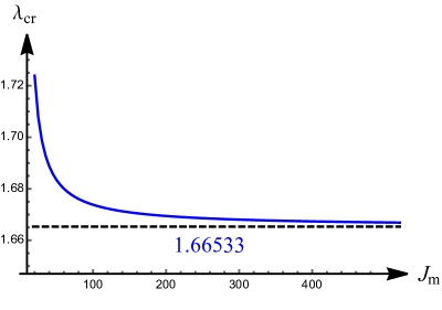
Figure 2: The graph shows $\lambda_{\textrm{cr}}$ as a function of the material extensibility $J_{\textrm{m}}$ for $\kappa\nu^{2}=50$. The dashed line corresponds to the asymptote as $J_{\textrm{m}}\rightarrow\infty$, when the critical stretch approaches $\lambda_{\textrm{cr}}=1.66533$ of the neo-Hookean material.

To verify the current formulation, we use a representative value $\kappa\nu^{2}=50$ and solve the bifurcation condition (59) for different values of $J_{\mathrm{m}}$ and compare results for $J_{\mathrm{m}}\rightarrow\infty$ with those reported in Liu and Dorfmann (2023). Figure 2 shows that the critical stretch $\lambda_{\textrm{cr}}$ is a monotonically decreasing function of $J_{\textrm{m}}$, indicating that a lower material extensibility limit delays the initiation of localized instability. As $J_{\textrm{m}}\rightarrow\infty$, the Gent model reduces to the neo-Hookean model and the critical stretch $\lambda_{\mathrm{cr}}\approx 1.66533$, which coincides with the results shown in Figure 2 in Liu and Dorfmann (2023).

For the Gent material (53), the conditions $\textrm{d}N/\textrm{d}\lambda=0$ and $\textrm{d}^{2}N/\textrm{d}\lambda^{2}=0$ determine the minimum values of $\kappa\nu^{2}$ for localized bifurcation as a function of $J_{\mathrm{m}}$. Figure 3 shows that $\left(\kappa\nu^{2}\right)_{\mathrm{min}}$ is a decreasing function of $J_{\mathrm{m}}$ and as $J_{\mathrm{m}}\rightarrow\infty$ approaches $\kappa\nu^{2}=29.5585$ of the neo-Hookean material. The graph also shows that there exists a critical value of $J_{\mathrm{m}}=J_{\mathrm{m}}^{*}$ when $\left(\kappa\nu^{2}\right)_{\mathrm{min}}\rightarrow\infty$. To determine this value we take the limit of $\kappa\nu^{2}\rightarrow\infty$ in the bifurcation condition (59) and obtain $\lambda=1.5$, which is then substitute back into $\textrm{d}N/\textrm{d}\lambda=0$ resulting in $J_{\textrm{m}}^{*}=0.58333$. For $J_{\textrm{m}}<J_{\mathrm{m}}^{*}$ localized bifurcation does not occur regardless the amount of the residual stress. This is similar to the options mentioned in Liu et al. (2019) on how to prevent localized bulging in inflated tubes.

In Figure 4 we present the dependence of the critical residual stress field $\left(\kappa\nu^{2}\right)_{\mathrm{cr}}$ on the amount of pre-stretch $\lambda$ for $J_{\mathrm{m}}=100$ and indicate $\kappa\nu^{2}=31.9855$ as the lowest value when localized bifurcation occurs at $\lambda_{\mathrm{m}}=2.0567$. Consistent with the results in Liu and Dorfmann (2023) , an increase in residual stress for constant stretch $\lambda<\lambda_{\mathrm{m}}$ initiates localized necking, for $\lambda>\lambda_{\mathrm{m}}$ localized bulging.

In Figure 5 we keep $\kappa\nu^{2}=31.9855$ constant to obtain $\lambda_{\mathrm{m}}$ as a function of $J_{\mathrm{m}}$. When the material extensibility limit $J_{\mathrm{m}}\rightarrow\infty$ the transition stretch $\lambda_{\mathrm{m}}$ approaches the value of the neo-Hookean model $\lambda_{\mathrm{m}}=2.1069$.

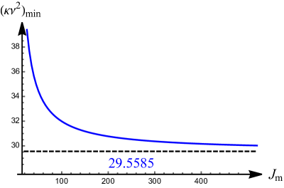
Figure 3: This figure shows $\left(\kappa\nu^{2}\right)_{\mathrm{min}}$ as a decreasing function of $J_{\mathrm{m}}$ and in the limit, as $J_{\mathrm{m}}\rightarrow\infty$, it approaches $\kappa\nu^{2}=29.5585$ of the neo-Hookean model.

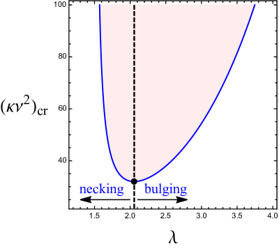
Figure 4: The relation between the critical residual stress $(\kappa\nu^{2})_{\textrm{cr}}$ and the pre-stretch $\lambda$ for $J_{\mathrm{m}}=100$. The black dot represents the lowest value $\kappa\nu^{2}=31.9855$ when the axial pre-stretch $\lambda_{\mathrm{m}}=2.0567$. An increase in residual stress with constant stretch $\lambda<\lambda_{\mathrm{m}}$ initiates localized necking, with $\lambda>\lambda_{\mathrm{m}}$ localized bulging.

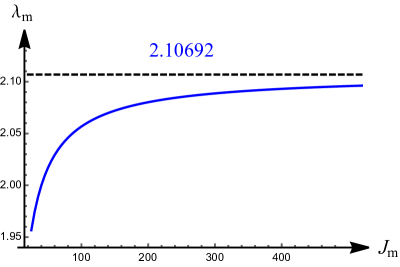
Figure 5: The transition stretch $\lambda_{\mathrm{m}}$ as a function of $J_{\mathrm{m}}$ for constant $\kappa\nu^{2}=31.9855$. When the material extensibility limit $J_{\mathrm{m}}\rightarrow\infty$, the stretch $\lambda_{\mathrm{m}}$ approaches the value of the neo-Hookean model $\lambda_{\mathrm{m}}=2.1069$.

5 Nonlinear one-dimensional model

We now focus our attention on using the one-dimensional model (51) to obtain a better understanding of the initiation and growth of a local bifurcation. First, we substitute (57), (58), (60), and (62) into (40) and (49) and use the results together with (61) to obtain the explicit form of (51). We use the centered finite difference method to solve the resulting nonlinear differential equation subject to well-posed boundary conditions. We discretize the half-length $[0,L]$ of the solid cylinder into $k$ intervals of step size $h=L/k$, determine the axial coordinate of node $j$ by $Z_{j}=jh$ and denote the corresponding stretch $\lambda\left(Z_{j}\right)$ by $\lambda_{j}$. The solution of the one-dimensional model is then reduced to the solution of a set of algebraic equations of the form

$$G^{\prime}(\lambda_{j})-\frac{1}{2}D^{\prime}(\lambda_{j})\left(\frac{\lambda_{j+1}-\lambda_{j-1}}{2h}\right)^{2}-D(\lambda_{j})\left(\frac{\lambda_{j+1}-2\lambda_{j}+\lambda_{j-1}}{h^{2}}\right)=0,\quad j=1,2,\cdots,k-1.$$ (64)

Suitable boundary conditions will be specified for the two loading conditions considered. In the first, the residual stress parameter $\nu$ is maintained constant, while the axial stretch is increased until a critical value is reached. In Liu and Dorfmann (2023) we found that with increasing stretch and with $\kappa\nu^{2}$ larger than a critical value, localized necking occurs. In the second case, we keep the pre-stretch constant and monotonically increase the residual stress $\nu$ until bifurcation occurs. Figure 4 in this paper and Figure 5 in Liu and Dorfmann (2023) show that the bifurcation changes character from necking to bulging as the pre-stretch becomes larger than a critical value.

In Yu and Fu (2023) it is shown that the one-dimensional model accurately describes the entire evolution process of bulging or necking for an inflated circular cylindrical tube of arbitrary wall thickness. In particular, the numerical results of a nonlinear finite element analysis are used to validate and verify the accurateness of the model.

5.1 Fixed residual stress

In this loading sequence the residual stress parameter $\nu$ is constant while the axial stretch is taken as the loading parameter. The one-dimensional model (51) only admits a localized solution if $D(\lambda)>0$. When integrating (49) from 0 to $A$ we recognize that at the location

$$R_{0}=\left(\frac{\lambda+6\kappa\lambda\nu-6\kappa\nu-\left(\left(\lambda\left(2\kappa\nu-1\right)-2\kappa\nu\right)^{2}-\dfrac{\lambda^{2}16\kappa(\lambda-1)J_{m}}{-\lambda J_{m}+\lambda^{3}-3\lambda+2}\right)^{1/2}}{8\kappa(\lambda-1)\nu}\right)^{1/2},$$ (65)

the modulus $\mathcal{A}_{2323}=0$, which generates a singularity in (40). In the linear analysis Liu and Dorfmann (2023), a similar singularity was classified as a regular singular point. Here, we use the same strategy and take the Cauchy principal value of the improper integral in the numerical integration scheme. We write

$$D(\lambda)=\int_{0}^{R_{0}-\delta}\left[\frac{1}{4}\mathcal{A}_{3232}\lambda^{-3}R^{3}-R\mathcal{A}_{2323}g^{2}(\lambda,R)\right]\mathrm{d}R+\int_{R_{0}+\delta}^{A}\left[\frac{1}{4}\mathcal{A}_{3232}\lambda^{-3}R^{3}-R\mathcal{A}_{2323}g^{2}(\lambda,R)\right]\mathrm{d}R$$ (66)

where $\delta$ is a small constant, here taken as $\delta=10^{-6}$.

To investigate if (51) admits a localized solution, we compute the changes of $D(\lambda)$ as a function $\lambda$ using $J_{\textrm{m}}=100,\kappa=0.5$ and $\nu=10$. Figure 6 shows that $D(\lambda)$ has two roots in the interval $1<\lambda<2.2$. Specifically, these are located at $\lambda_{\textrm{t1}}=1.40991$ and $\lambda_{\textrm{t2}}=1.85396$ and compare to the critical stretch $\lambda_{\textrm{cr}}=1.67381$, where localized bifurcation occurs. The mathematical nature of the current problem is identical to the one obtained by replacing the residual stress by a surface tension to generate localization in inflated tubes. There, it has been shown that the bifurcation nature is subcritical, a condition of bifurcation we adopt here as well Fu et al. (2008); Emery and Fu (2021b); Emery (2023); Ye et al. (2020); Fu et al. (2021); Yu and Fu (2023).

In infinitely long cylindrical solids or tubes it is customary to denote the stretch at infinity by $\lambda_{\infty}$. When localized bifurcation occurs, the stretch no longer remains uniform and becomes a function of $Z$. For long cylindrical solids of half-length $L$, the exact value of $\lambda_{\mathrm{L}}$ has an exponentially small difference from $\lambda_{\infty}$, a difference we neglect in the following Wang and Fu (2020).

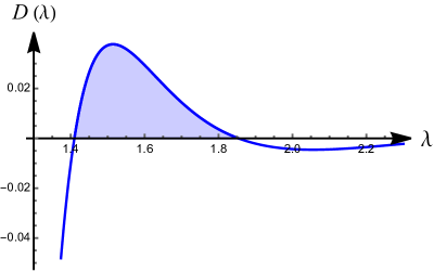
Figure 6: The dependence of $D(\lambda)$ on $\lambda$ when $J_{\textrm{m}}=100,\kappa=0.5$ and $\nu=10$ with roots located at $\lambda_{\textrm{t1}}=1.40991$ and $\lambda_{\textrm{t2}}=1.85396$.

Based on the principle of translational invariance, we assume that localization initiates at $Z=0$. Then, it is convenient to use the difference between $\lambda(0)$ and $\lambda_{\infty}$ to identify the bifurcation nature. For subcritical bifurcation, the loading parameter $\lambda_{\infty}$ will be less than $\lambda_{\textrm{cr}}$ or, equivalently, $a_{\infty}>a_{\mathrm{cr}}$. According to the Noether’s theorem Noether (1918), the evolution of $\lambda(0)$ in the post-bifurcation regime can be obtained by solving

$$G(\lambda(0))=G(\lambda_{\infty}),$$ (67)

where the form of $G(\lambda)$ is given in (61). Note that (67) can also be obtained from (52) by setting the derivative $\lambda^{\prime}=0$.

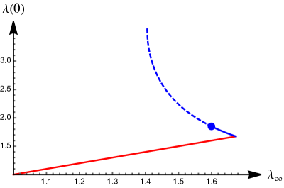
Figure 7: The bifurcation diagram for $J_{\textrm{m}}=100$, $\kappa=0.5$ and $\nu=10$. The homogeneous response $\lambda_{\infty}=\lambda(0)$ is shown in red, while the non-trivial solution is depicted in blue.

The bifurcation diagram for $J_{\textrm{m}}=100$, $\kappa=0.5$ and $\nu=10$ is obtained from (67) and is shown in Figure 7. The homogeneous response $\lambda_{\infty}=\lambda(0)$ is shown in red, while the non-trivial solution is depicted in blue. Bifurcation occurs when $\lambda_{\infty}=\lambda(0)=1.67381$ and, subsequently, $\lambda(0)$ increases with $\lambda_{\infty}$ getting smaller. The deformed radius given by $a(Z)=\lambda(Z)^{-1/2}$, indicates localized necking. The blue dot, in particular, corresponds to $\lambda_{\infty}=1.59836$ and $\lambda(0)=\lambda_{\textrm{t2}}=1.85396$, the latter being a root of $D(\lambda)$, see Figure 6. A further reduction in $\lambda_{\infty}$ results in $D(\lambda)<0$ and model (51) no longer admits a localized solution.

To obtain the radius as a function of $Z$ in the post-bifurcation regime, we numerically solve equation (51) subject to the boundary conditions

$$\lambda(0)=\lambda_{0},\quad\lambda^{\prime}(0)=0,$$ (68)

where $\lambda_{0}$ is obtained from (67) for given $\lambda_{\infty}$ and $\lambda^{\prime}(0)=0$ implies symmetry in the deformation. We use the finite difference method with $k=50$ intervals and Newton’s method to solve the algebraic equations (64) for representative values $\lambda_{\infty}=1.65381,1.62381$ and $1.60381$. The deformed radius $a(Z)=\lambda(Z)^{-1/2}$ is shown in Figure 8 for different $\lambda_{\infty}$.

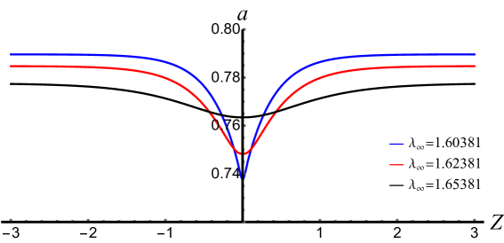
Figure 8: Dependence of the deformed radius $a$ on $Z$ for various values of $\lambda_{\infty}$. For clarity of presentation, we show localized necking from $Z=-3$ to $Z=3$.

In Liu and Dorfmann (2023) we characterized localized bifurcation, the corresponding change in radius and the propagation as a the two-phase deformation consisting of necked and bulged regions. These are connected by a transition zone, which simply translates along the axial direction. During propagation, the stretches of each phase are unchanged and are determined by Maxwell’s equal-area rule. The change in radius is visualized by the solid/dashed blue curve in Figure 7 and is completed once the Maxwell values of stretch are reached, i.e. the end of the blue curve. The Maxwell values of stretch of the bulged and necked regions are denoted by $\lambda_{\textrm{p1}}$, $\lambda_{\textrm{p2}}$, respectively, and are shown as a function of the material extensibility limit $J_{\mathrm{m}}$ in Figure 9. We find that $\lambda_{\textrm{p2}}$ is a monotonically increasing function, while $\lambda_{\textrm{p1}}$ has the opposite behavior.

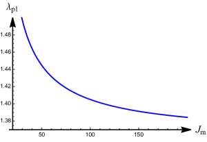
(a) The stretch at the bulged region as a function of $J_{\textrm{m}}$.

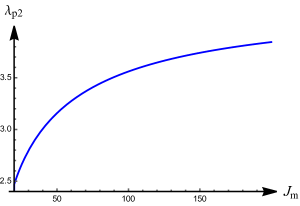
(b) The stretch at the necked region as a function of $J_{\textrm{m}}$.

Figure 9: The dependence of two Maxwell stretches on $J_{\textrm{m}}$. We understand that in the Maxwell state the deformation is composed of two uniform deformations joined by a transition zone, and we label this by a two-phase deformation as well.

We also find that the magnitude of the local minimum of $D(\lambda)$ depends on $J_{\textrm{m}}$, see Figure 6. For what follows, it is interesting to determine the value $J_{\textrm{m}}$ for which the local minimum of $D(\lambda)=0$. This is given by the solution of

$$\frac{\textrm{d}D(\lambda)}{\textrm{d}\lambda}=0,\quad D(\lambda)=0,$$ (69)

resulting in $J^{\mathrm{cr}}_{\mathrm{m}}=33.5637$ with the root increasing to $\lambda_{\mathrm{t2}}=2.03201$. Both Maxwell stretches now lie in the interval $(\lambda_{\textrm{t1}},\lambda_{\textrm{t2}})$ as $J_{\mathrm{m}}<J_{\mathrm{m}}^{\mathrm{cr}}$ and the one-dimensional model will be able to capture the necking initiation and growth evolution until the two-phase deformation develops, i.e. $D(\lambda)$ is always positive.

Take $J_{\textrm{m}}<J^{\textrm{cr}}_{\textrm{m}}=20,\kappa=0.5,\nu=10$ and explore the necking evolution using the model (51). Figure 10 illustrates the relation between $D(\lambda)$ and $\lambda$ with the roots now located at $\lambda_{\textrm{t1}}=1.4164$ and $\lambda_{\textrm{t2}}=2.64427$. The corresponding Maxwell values of stretch are calculated as $\lambda_{\textrm{p1}}=1.56876>\lambda_{\textrm{t1}}$ and $\lambda_{\textrm{p2}}=2.46839<\lambda_{\textrm{t2}}$. The bifurcation diagram is again obtained from (67) and is shown in Figure 11, where the deformation is homogeneous until the value $\lambda_{\infty}=\lambda(0)=\lambda_{\textrm{cr}}=1.72389$ is reached. The blue curve shows the evolution of the necking amplitude, which terminates at the Maxwell values of stretch.

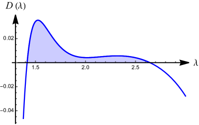
Figure 10: The dependence of $D(\lambda)$ on $\lambda$ when $J_{\textrm{m}}=20$, $\kappa=0.5$, and $\nu=10$ with the roots located at $\lambda_{\textrm{t1}}=1.4164$ and $\lambda_{\textrm{t2}}=2.64427$.

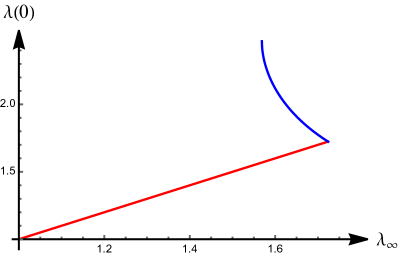
Figure 11: The bifurcation diagram when $J_{\textrm{m}}=20$, $\kappa=0.5$, and $\nu=10$. The red line represents the homogeneous deformation, the blue depicts the evolution of necking.

To calculate the axial stretch $\lambda(Z)$ for different values of $\lambda_{\infty}$, we follow the procedure used to obtain the graphs in Figure 8. Here, we consider $\lambda_{\infty}=1.70389,1.62389,1.57876$ and $1.56876$ and show the corresponding changes of radius $a(Z)=\lambda^{-1/2}(Z)$ in Figure 12. For the special case where the value of $\lambda_{\infty}$ is equal to the Maxwell stretch $\lambda_{\textrm{p1}}=1.56876$, the one-dimensional model (51) is capable to simulate the initiation and the entire growth process.

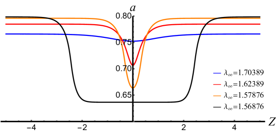
Figure 12: The evolution of the necking profiles for different values of $\lambda_{\infty}$ with $J_{\textrm{m}}=20$, $\kappa=0.5$, and $\nu=10$. For clarity of presentation we restrict attention to the region $-5\leqslant Z\leqslant 5$.

The left image in Figure 13 shows the axial force $N$ against the stretch $\lambda(0)$ for $J_{\mathrm{m}}=20,\kappa=0.5,\nu=10$ before the Maxwell stage, the right image is a magnified view. The homogeneous deformation (58) is depicted by the blue curve up to $\lambda_{\mathrm{cr}}=1.67381$, the remaining part is obtained using (67). The red curve, given by (58), is unstable and shown for reference only deBotton et al. (2013); Liu et al. (2023).

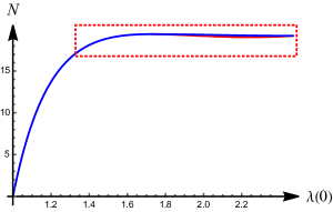
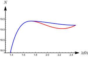
Figure 13: The axial force $N$ versus the axial stretch $\lambda(0)$ as $J_{\textrm{m}}=20$, $\kappa=0.5$, and $\nu=10$. The right image is a magnified view. The homogeneous deformation (58) is depicted by the blue curve up to $\lambda_{\mathrm{cr}}=1.67381$, the remaining part is obtained using (67). The red curve, given by (58), is unstable and shown for reference only.

5.2 Fixed axial length

For the second loading scenario we keep the pre-stretch constant and use $\nu$ as the loading parameter. It is shown in Liu and Dorfmann (2023) that, depending on the amount of pre-stretch, localized necking or bulging occurs for a residual stress larger than some critical value.

In Figure 4 we define $\lambda_{\mathrm{m}}=2.0567$ and show that an increase in residual stress with constant pre-stretch $\lambda<\lambda_{\mathrm{m}}$ initiates localized necking, with $\lambda>\lambda_{\mathrm{m}}$ localized bulging. We now use the one-dimensional model to validate this finding.

The fixed length condition requires that by

$$\int_{0}^{L}\lambda(Z)\textrm{d}Z=\lambda_{\textrm{f}}L,$$ (70)

where the constant pre-stretch $\lambda_{\textrm{f}}>1$. Applying the discretization procedure results in

$$\frac{1}{2}\lambda(0)+\sum_{j=1}^{k-1}\lambda(j)+\frac{1}{2}\lambda(k)-\frac{\lambda_{\textrm{f}}}{h}L=0,$$ (71)

where $k$ is the number of nodes and $h=L/k$ is the step size. To formulate a well-defined system, two boundary conditions are required. Similar to the previous loading scenario, we neglect the exponentially small error Wang and Fu (2020) and use

$$\lambda^{\prime}(0)=0,\quad\lambda^{\prime}(L)=0,$$ (72)

which have the discretized forms

$$\frac{\lambda_{1}-\lambda_{-1}}{2h}=0,\quad\frac{\lambda_{k+1}-\lambda_{k-1}}{2h}=0.$$ (73)

As $\lambda(0)$ and $\lambda_{\infty}$ are both unknown, we rewrite (64) in the form

$$G^{\prime}(\lambda_{j})-\frac{1}{2}D^{\prime}(\lambda_{j})\left(\frac{\lambda_{j+1}-\lambda_{j-1}}{2h}\right)^{2}-D(\lambda_{j})\left(\frac{\lambda_{j+1}-2\lambda_{j}+\lambda_{j-1}}{h^{2}}\right)=0,\quad j=0,1,\cdots,k,$$ (74)

which, when combined with (71), result in $(k+2)$ algebraic equations for $\lambda_{j},j=0,\dots,k$ and $\lambda_{\infty}$.

Consider a cylindrical solid with material extensibility limit $J_{\textrm{m}}=100$, $\kappa=0.5$ and constant pre-stretch $\lambda_{\textrm{f}}=1.9$. Bifurcation occurs when the residual stress parameter $\nu_{\textrm{cr}}=8.17618$ or, equivalently $(\kappa\nu^{2})_{\mathrm{cr}}=33.425$, see Figure 4. In addition, it shows that the axial pre-stretch $\lambda_{\textrm{f}}$ is less than the transition value $\lambda_{\textrm{m}}=2.0567$ indicating localized necking.

To use the one-dimensional model (51) we first compute the changes of $D(\lambda)$ as a function of $\lambda$ and show the dependence in Figure 14. The two roots are calculated as $\lambda_{\textrm{t1}}=1.42367$ and $\lambda_{\textrm{t2}}=3.08483$ with $\lambda_{\textrm{t1}}<\lambda_{\textrm{f}}<\lambda_{\textrm{t2}}$ such that model (51) admits a localized solution.

For a subcritical bifurcation, the loading parameter after bifurcation decreases and we take $\nu=\nu_{\textrm{cr}}-0.05=8.12618$. To find a solution, we use the starting value $\lambda_{\infty}=1.899$, which is slightly lower than $\lambda_{\textrm{f}}$ and obtain $\lambda_{0}$ from (67). Then, we numerically solve (51) with (70) and adjust the value of $\lambda_{\infty}$ until equation (70) is satisfied. The profile of the solid cylinder in the post-bifurcation state is given by $a(Z)=\lambda(Z)^{-1/2}$ and is depicted in Figure 15. The solution clearly shows that necking has occurred.

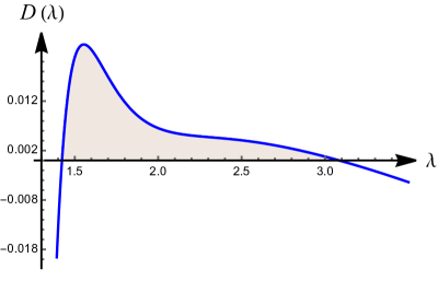
Figure 14: The dependence of $D(\lambda)$ on $\lambda$ when the material extensibility $J_{\textrm{m}}=100$, $\kappa=0.5$ and $\nu=8.17618$. The two roots are located at $\lambda_{\textrm{t1}}=1.42367$ and $\lambda_{\textrm{t2}}=3.08483$.

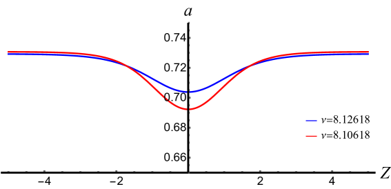
Figure 15: The blue and red curves represent the post-bifurcation profiles of a solid cylinder with constant pre-stretch $\lambda_{\textrm{f}}=1.9$, $J_{\textrm{m}}=100$, $\kappa=0.5$. The residual stress parameters are $\nu=8.12618$ and $\nu=8.10618$, respectively.

For the last illustration, we consider a cylindrical solid with constant pre-stretch $\lambda_{\mathrm{f}}>\lambda_{\mathrm{m}}$, where $\lambda_{\mathrm{m}}=2.0567$. Figure 4 shows that an increase in residual stress initiates localized bulging. For $J_{\textrm{m}}=100,\kappa=0.5$ and $\lambda_{\textrm{f}}=2.2$ localized bifurcation occurs when $\nu_{\textrm{cr}}=8.09505$. Figure 16 shows the dependence of $D(\lambda)$ on $\lambda$ and the two roots located at $\lambda_{\textrm{t1}}=1.42471$ and $\lambda_{\textrm{t2}}=3.06389$. Hence, the one-dimensional model (51) admits a localized solution for a constant pre-stretch $\lambda_{\textrm{t1}}<\lambda_{\mathrm{f}}<\lambda_{\textrm{t2}}$.

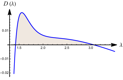
Figure 16: The dependence of $D(\lambda)$ on $\lambda$ as $J_{\textrm{m}}=100$, $\kappa=0.5$, and $\nu=8.09505$. The two roots are located at $\lambda_{\textrm{t1}}=1.42471$ and $\lambda_{\textrm{t2}}=3.06389$.

Figure 17 displays the profiles of the cylinder for different values of the residual stress parameter $\nu$. It clearly shows that bulging has occurred, validating the results obtained in the linear bifurcation analysis Liu and Dorfmann (2023).

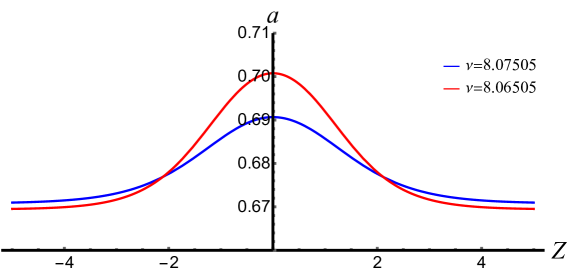
Figure 17: The blue and red curves represent the bulging profiles of a solid cylinder with constant pre-stretch $\lambda_{\textrm{f}}=2.2$, $J_{\textrm{m}}=100$, $\kappa=0.5$. The residual stress parameters are $\nu=8.07505$ and $\nu=8.06505$, respectively.

6 Conclusions

Instabilities in the form of periodic or localized pattern in residually stressed materials have been observed in biological structures and in man-made devices. In particular, the residual stress in biological materials arises due to growth and remodeling and has a signifiant influence on the mechanical response, as shown in, for example, Holzapfel et al. (2000). In manufacturing, residual stress may improve material performance or cause weaknesses and possibly a reduction in the life of components Melnikov et al. (2021).

The bifurcation behavior leading to the formation of periodic pattern is based on the theory of incremental deformations superimposed on a known finitely deformed configuration Haughton and Ogden (1979a, b). Contrasting, the analysis of localized instabilities, such as necking or bulging, focuses on initiation, growth and propagation. They play a role in nanotubes that bridge neighboring cells Veranic et al. (2008) and in trauma induced beading instabilities responsible for damage of axons Hemphill et al. (2015). Recently, the effect of surface tension to initiate localized instabilities in soft solids has been recognized Fu et al. (2021), and the one-dimensional theory can be used to better understand this phenomenon. The theory presented in this paper can also be extended to evaluate the effect of residual stress on localized pattern formation in liquid crystal elastomers Li et al. (2022) and in the formation and propagation of abdominal aortic aneurysms Ahamed et al. (2016).

We focused on a residually stressed Gent material and investigated localized bifurcation of a circular cylindrical solid subject to axial stretch. We discussed the dimensional reduction of the total potential energy functional and used the resulting one-dimensional model to analyze the post-bifurcation behavior.

Two loading scenarios were considered. In the first, we keep the residual stress constant and monotonically increase the axial stretch until localized bifurcation occurs. In the second, we apply a constant pre-stretch and use the residual stress as the loading parameter.

The bifurcation diagram of the first loading sequence shows that the deformation is homogeneous until the critical stretch is reached. This is followed by the non-trivial solution during which the axial stretch of the unstable region increases compared to the far end value. We plot the radial deformation as a function of the axial position and show that localized necking occurs. We also optimize the material extensibility to show that the solution of the one-dimensional model is valid until the Maxwell values of stretch are reached.

For the second loading sequence we determine the transition stretch $\lambda_{\mathrm{m}}$, which distinguishes between necking or bulging modes. Specifically, we find that an increase in residual stress with constant stretch $\lambda<\lambda_{\mathrm{m}}$ initiates localized necking, an axial stretch $\lambda>\lambda_{\mathrm{m}}$ leads to localized bulging. The corresponding axial profiles of the axisymmetric solid in the post-bifurcation state are shown.

Funding

This work was supported by the National Natural Science Foundation of China (Project Nos 12072227 and 12021002).

ORCID iD

Yang Liu https://orcid.org/0000-0001-9517-3833
Xiang Yu https://orcid.org/0000-0002-3378-6340
Luis Dorfmann https://orcid.org/0000-0002-9665-0272

References

- Mallock (1890) Mallock, A. Note on the instability of India-rubber tubes and balloons when distended by fluid pressure. Proc R Soc Lond 1890; 49:458–463.
- Fu and Ogden (1999) Fu, YB, and Ogden, RW. Nonlinear stability analysis of pre-stressed elastic bodies Continuum Mech Thermodyn 1999; 11:141–172.
- Ogden (1997) Ogden, RW. Non-linear elastic deformations. New York: Dover Publications, 1997.
- Fu (2001) Fu, YB. Perturbation methods and nonlinear stability analysis, in: Fu, Y.B., Ogden, R.W. (Eds.), Nonlinear elasticity: Theory and Applications. Cambridge University Press, Cambridge, 2001
- Fu et al. (2008) Fu, YB, Pearce, SP, and Liu, KK. Post-bifurcation analysis of a thin-walled hyperelastic tube under inflation. Int J Non-linear Mech 2008; 43:697–706.
- Pearce and Fu (2010) Pearce, SP and Fu, YB. Characterisation and stability of localised bulging/necking in inflated membrane tubes. IMA J Appl Math 2010; 75:581–602.
- Fu et al. (2016) Fu, YB, Liu, JL, and Francisco, GS. Localized bulging in an inflated cylindrical tube of arbitrary thickness - the effect of bending stiffness. J Mech Phys Solids 2016; 90:45–60.
- Yu and Fu (2022) Yu, X, and Fu, Y. An analytic derivation of the bifurcation conditions for localization in hyperelastic tubes and sheets Z Angew Math Phys 2022; 73:1–16.
- Fu et al. (2018) Fu, YB, Dorfmann, L, and Xie, Y-X. Localized necking of a dielectric membrane. Extreme Mech Lett 2018; 21:44–48.
- Ye et al. (2020) Ye, Y, Liu, Y and Fu, YB. Weakly nonlinear analysis of localized bulging of an inflated hyperelastic tube of arbitrary wall thickness. J Mech Phys Solids 2020; 135:103804.
- Wang et al. (2019) Wang, S, Guo, Z, Zhou, L, Li, L, and Fu, YB. An experimental study of localized bulging in inflated cylindrical tubes guided by newly emerged analytical results. J Mech Phys Solids 2019; 124:536–554.
- Guo et al. (2022) Guo, Z, Wang, S and Fu, Y. Localized bulging of an inflated rubber tube with fixed ends. Phil Trans R Soc A 2022; 380:20210318.
- Audoly and Hutchinson (2016) Audoly, B and Hutchinson, JW. Analysis of necking based on a one-dimensional model. J Mech Phys Solids 2016; 97:68–91.
- Lestringant and Audoly (2018) Lestringant, B, and Audoly, B. A diffuse interface model for the analysis of propagating bulges in cylindrical balloons. Proc R Soc A 2018; 474:2018333.
- Audoly and Hutchinson (2019) Audoly, B, and Hutchinson, J.W. One-dimensional modeling of necking in rate-dependent materials. J Mech Phys Solids 2019; 123:149–1711.
- Lestringant and Audoly (2020a) Lestringant, B, and Audoly, B. Asymptotically exact strain-gradient models for nonlinear slender elastic structures: A systematic derivation method J Mech Phys Solids 2020; 136:103730.
- Lestringant and Audoly (2020) Lestringant, B, and Audoly, B. A one-dimensional model for elasto-capillary necking. Proc R Soc A 2020; 476:20200337.
- Yu and Fu (2023) Yu, X, and Fu, Y. A one-dimensional model for axisymmetric deformations of an inflated hyperelastic tube of finite wall thickness. J Mech Phys Solids 2023; 175:105276.
- Liu and Dorfmann (2023) Liu, Y and Dorfmann, L. Localized necking and bulging of finitely deformed residually stressed solid cylinder. Math Mech Solids 2023; in press: DOI: 10.1177/10812865231186951.
- Rajagopal and Wineman (2024) Rajagopal, KR and Wineman A. Residual stress and material symmetry. Int J Eng Sci 2024; 197:104013.
- Hoger (1993) Hoger A. The constitutive equation for finite deformations of a transversely isotropic hyperelastic material with residual-stress. J Elasticity 1993; 33:107–118.
- Holzapfel and Ogden (2010) Holzapfel, GA and Ogden, RW. Modelling the layer-specific 3D residual stresses in arteries, with an application to the human aorta. J R Soc Interface 2010; 7:787–799.
- Hoger (1985) Hoger A. On the residual stress possible in an elastic body with material symmetry. Arch Ration Mech Anal 1985; 88:271–290.
- Wolfram Research Inc. (2019) Wolfram Research Inc. 2019. Mathematica: version 12. Champaign, IL: Wolfram Research Inc.
- Emery and Fu (2021b) Emery, DR and Fu, YB. Post-bifurcation behaviour of elasto-capillary necking and bulging in soft tube. Proc. R. Soc. A 2021; 477:20210311.
- Emery (2023) Emery, DR. Elasto-capillary necking, bulging and Maxwell states in soft compressible cylinders. Int J Non-linear Mech 2023; 148:104276.
- Fu et al. (2021) Fu, YB, Jin, L and Goriely, A. Necking, beading, and bulging in soft elastic cylinders. J Mech Phys Solids 2021; 147:104250.
- Liu et al. (2019) Liu, Y, Ye, Y, Althobaiti, A and Xie, Y-X. Prevention of localized bulging in an inflated bilayer tube. Int J Mech Sci 2019; 153–154:359–368.
- Melnikov et al. (2021) Melnikov, A, Ogden, RW, Dorfmann, L and Merodio, J. Bifurcation analysis of elastic residually stressed circular cylindrical tubes. Int J Solids Struct 2021; 226–227:111062.
- Melnikov et al. (2022) Melnikov, A, Merodio, J, Bustamante, R and Dorfmann, L. Bifurcation analysis of residually stressed neo-Hookean and Ogden electroelastic tubes. Phil Trans R Soc A, 2022; 380:20210331.
- Wang and Fu (2020) Wang, M and Fu, YB. Necking of a hyperelastic solid cylinder under axial stretching: Evaluation of the infinite-length approximation. Int J Eng Sci 2020; 159:103432.
- Noether (1918) Noether, E. Invariante Variationsprobleme. Nachrichten von der Gesellschaft der Wissenschaften zu Göttingen. Mathematisch-Physikalische Klasse 1918; 235–257.
- deBotton et al. (2013) deBotton, G, Bustamante, R and Dorfmann, A. Axisymmetric bifurcations of thick spherical shells under inflation and compression. Int J Solids Struct 2013; 50:403–413.
- Liu et al. (2023) Liu, Y, Yang, L and Xie, Y-X. Inflation-induced bulge initiation and evolution in graded cylindrical tubes of arbitrary thickness. Mech Mater 2023; 178:104561.
- Holzapfel et al. (2000) Holzapfel, GA, Gasser, TC and Ogden, RW. A new constitutive framework for arterial wall mechanics and a comparative study of material models. J Elast 2000; 61:1–48.
- Haughton and Ogden (1979a) Haughton, DM and Ogden, RW. Bifurcation of inflated circular cylinders of elastic material under axial loading—I. Membrane theory for thin-walled tubes. J Mech Phys Solids 1979a; 27:179–212.
- Haughton and Ogden (1979b) Haughton, DM and Ogden, R.W. Bifurcation of inflated circular cylinders of elastic material under axial loading—II. Exact theory for thick-walled tubes. J Mech Phys Solids 1979b; 27:489–512.
- Veranic et al. (2008) Veranič, P, Lokar, M, Schütz, GJ, Weghuber, J, Wieser, S, Hägerstrand, H, Kralj-Iglič, V and Iglič, A. Different types of cell-to-cell connections mediated by nanotubular structures Biophys J 2008; 95:4416–4425.
- Hemphill et al. (2015) Hemphill, MA, Dauth, S, Yu, CJ, Dabiri, BE and Parker, KK. Traumatic brain injury and the neuronal microenvironment: a potential role for neuropathological mechanotransduction. Neuron 2015; 85:1177–1192.
- Li et al. (2022) Li, Min, Yan, Y, Xu, S, Wang, G, Wu, X, Fenh, X-Q. Surface effect on the necking of hyperelastic materials. Curr Appl Phys 2022, 38, 91–98.
- Ahamed et al. (2016) Ahamed, T, Dorfmann, L and Ogden, RW. Modeling of residually stressed materials with applications to AAA. J Mech Behav Biomed Mater 2016; 61:221-234.