Error bounds for rank-one DNN reformulation of QAP and DC exact penalty approach

Abstract

This paper concerns the quadratic assignment problem (QAP), a class of challenging combinatorial optimization problems. We provide an equivalent rank-one doubly nonnegative (DNN) reformulation with fewer equality constraints, and derive the local error bounds for its feasible set. By leveraging these error bounds, we prove that the penalty problem induced by the difference of convexity (DC) reformulation of the rank-one constraint is a global exact penalty, and so is the penalty problem for its Burer-Monteiro (BM) factorization. As a byproduct, we verify that the penalty problem for the rank-one DNN reformulation proposed in Jiang21 is a global exact penalty without the calmness assumption. Then, we develop a continuous relaxation approach by seeking approximate stationary points of a finite number of penalty problems for the BM factorization with an augmented Lagrangian method, whose asymptotic convergence certificate is also provided under a mild condition. Numerical comparison with Gurobi for 131 benchmark instances validates the efficiency of the proposed DC exact penalty approach.

1 Introduction

Quadratic assignment problem (QAP) is a fundamental problem in location theory, which allocates $n$ facilities to $n$ locations and minimizes a quadratic objective function on the distance between the locations and the flow between the facilities. Let $\mathbb{R}^{n\times q}$ represent the space consisting of all $n\times q$ real matrices, equipped with the trace inner product $\langle\cdot,\cdot\rangle$ and its induced Frobenius norm $\|\cdot\|_{F}$. For the given data matrices $A,B\in\mathbb{R}^{n\times n}$ and $C\in\mathbb{R}^{n\times n}$, the QAP is formulated as

$$\min_{X\in\mathcal{P}_{\!n}}\langle X,AXB+C\rangle,$$ (1)

where $\mathcal{P}_{\!n}\!:=\{X\in\{0,1\}^{n\times n}\ |\ Xe_{n}=e_{n},X^{\top}e_{n}=e_{n}\}$ denotes the set of all $n\times n$ permutation matrices, and $e_{n}$ is the vector of all ones of $\mathbb{R}^{n}$. Note that the global (or local) optimal solution set of problem (1) keeps unchanged when $A$ is replaced by $A-\min_{i,j}A_{ij}e_{n}e_{n}^{\top}$ (similarly for $B$ or $C$). With such a preprocessing, we can assume that the data matrices $A,B$ and $C$ involved in (1) are nonnegative.

The QAP has wide applications in facility layout, chip design, scheduling, manufacturing, etc; see Burkard13 ; Drezner15 and the references therein. Some generalizations, such as the cubic, quartic and general N-adic assignment problems, are also investigated in Lawler63 ; Burkard94 . When $C=0$, problem (1) can equivalently be written as

$$\min_{X\in\mathcal{P}_{n}}\|A^{\top}X+XB\|_{F}^{2},$$ (2)

which has a wide application in pattern recognition and machine vision Conte14 , and also covers the bandwidth minimization problem (see (JiangLW16, , section 7)) appearing frequently in sparse matrix computations, circuit design, and VLSI layout Chinn82 ; Lai99 .

Due to the dimension restriction, it is impractical to solve the QAP exactly; for example, obtaining an exact solution with the branch-and-bound method for $n=30$ is still considered to be computationally challenging. This work aims to develop an effective continuous relaxation approach to seek a high-quality even exact optimal solution for problem (1).

1.1 Related works

In this section, we mainly review continuous relaxation approaches to yield good approximate solutions with desirable lower bounds or feasible solutions with desirable upper bounds, and will not introduce the exact methods (see, e.g., Adams07 ; Fischetti12 ) and the heuristic methods (see, e.g., Stutzle06 ; Pardalos94 ; Taillard91 ; Burkard13 ). By the Birkhoff-von Neumann theorem, the convex hull of $\mathcal{P}_{\!n}$ is the set of doubly stochastic matrices $\mathcal{D}_{\!n}$. The first class of continuous relaxation methods is developed by the quadratic program

$$\min_{X\in\mathcal{D}_{\!n}}\langle X,AXB+C\rangle.$$ (3)

For example, Xia Xia10 proposed a Lagrangian smoothing algorithm by solving a sequence of $L_{2}$-regularization subproblems of (3) with dynamically decreasing regularization parameters. Motivated by $\mathcal{P}_{\!n}=\mathcal{D}_{\!n}\cap\{X\!\in\mathbb{R}^{n\times n}\ |\ \|X\|_{0}=n\}$, where $\|X\|_{0}$ denotes the number of nonzero entries of $X$, Jiang et al. JiangLW16 considered that the $L_{0}$-norm regularization problem of (3), which was shown to possess the same global optimal solution set as (3), and developed a regularization algorithm by the approximation model obtained by replacing the zero-norm $\|X\|_{0}$ with the $L_{p}$-norm. To deal with the nonconvex objective function of (3), Zaslavskiy et al. Zaslavskiy09 and Liu et al. LiuQiao12 also proposed path-following algorithms by solving a sequence of convex combinations of convex and concave optimization problems over $\mathcal{D}_{n}$.

The second class is proposed by the fact that $\mathcal{P}_{\!n}\!=\!\{X\!\in\mathbb{R}_{+}^{n\times n}\ |\ X^{\top}X=I_{n}\}$, where $\mathbb{R}_{+}^{n\times n}$ denotes the nonnegative cone of $\mathbb{R}^{n\times n}$ and $I_{n}$ is an $n\times n$ identity matrix. Wen and Yin Wen13 first reformulated problem (1) with $C=0$ as

$$\min_{X\in\mathbb{R}^{n\times n}}\Big{\{}\langle A,(X\odot X)B(X\odot X)^{\top}\rangle\ \ {\rm s.t.}\ \ X^{\top}X=I_{n},\,X\in\mathbb{R}_{+}^{n\times n}\Big{\}},$$

where “$\odot$” denotes the Hadamard product of two matrices, and proposed an efficient algorithm by applying the augmented Lagrangian method (ALM) to handle the nonnegative constraint $X\in\mathbb{R}_{+}^{n\times n}$, in which every ALM subproblem is solved with a nonmonotone line-search Riemannian gradient descent method. Recently, for the following general nonnegative orthogonal problem

$$\min_{X\in\mathbb{R}^{n\times r}}\Big{\{}f(X)\ \ {\rm s.t.}\ \ X^{\top}X=I_{r},\,X\in\mathbb{R}_{+}^{n\times r}\Big{\}}$$ (4)

where $f\!:\mathbb{R}^{n\times r}\to\mathbb{R}$ is a smooth function, Jiang et al. JiangM22 reformulated it as

$$\min_{X\in\mathbb{R}^{n\times r}}\Big{\{}f(X)\ \ {\rm s.t.}\ \ \|XV\|_{F}=1,\,X\in\mathcal{OB}_{+}^{n,r}\Big{\}}$$

where $\mathcal{OB}_{+}^{n,r}\!:=\!\{X\!\in\mathbb{R}_{+}^{n\times r}\,|\,\|X_{j}\|=1,\,j=1,\ldots,r\}$ and $V\!\in\mathbb{R}^{n\times r}$ is a constant matrix satisfying a certain condition, achieved a class of exact penalty models induced by the constraint $\|XV\|_{F}=1$, and developed a practical exact penalty algorithm; while Qian et al. QianPanXiao22 proved that the penalty problem induced by the $\ell_{1}$-norm distance from the nonnegative cone $\mathbb{R}_{+}^{n\times r}$ is a global exact penalty and so is its Moreau envelope under a mild condition, and then developed an efficient algorithm by the Moreau envelope exact penalty, in which the penalty subproblems are solved with a nonmonotone line-search Riemannian gradient descent method. Different from the first class, this class of relaxation approaches captures a certain surface information on $\mathcal{P}_{\!n}$ by means of the orthogonal manifold.

The third class is developed by the outer approximation to the completely positive cone $\mathcal{C}_{p}^{*}\!:=\!{\rm conv}\{zz^{\top}\,|\,z\in\mathbb{R}^{p}_{+}\}$ with $p=n^{2}$, which is the positive dual of the closed convex cone $\{Y\!\in\mathbb{S}^{p}\ |\ \xi^{\top}Y\xi\geq 0\ \ \forall\xi\in\mathbb{R}_{+}^{p}\}$. In this work, $\mathbb{S}^{p}$ represents the set of all $p\times p$ real symmetric matrices, and $\mathbb{S}_{+}^{p}$ means the cone consisting of all positive semidefinite matrices in $\mathbb{S}^{p}$. Inspired by the work Anstreicher2000 , Povh and Rendl Povh09 first proved that (1) is equivalent to a completely positive conic program

$$\min_{Y\!\in\mathbb{S}^{p}}\ \langle B\otimes A+{\rm Diag}({\rm vec}(C)),Y\rangle$$

$$\ \ {\rm s.t.}\ \ {\textstyle\sum_{i=1}^{n}}{Y^{ii}}=I_{n},\ \langle I_{n},Y^{ij}\rangle=\delta_{ij},\ \ \forall i,j\in[n],$$ (5)

$$\qquad\ \ \langle e_{p}e_{p}^{\top},Y\rangle=p,\ Y\!\in\mathcal{C}_{p}^{*}$$

in the sense that they have the same optimal value, where “$\otimes$” means the Kronecker product of two matrices, $\delta_{ij}=1$ if $i=j$, otherwise $\delta_{ij}=0$, and for each $Y\!\in\mathbb{S}^{p}$, $Y^{ij}\in\mathbb{R}^{n\times n}$ with $i,j\in[n]$ denotes the $(i,j)$-th block of $Y$. Since the closed convex cone $\mathcal{C}_{p}^{*}$ is numerically intractable, inspired by the work Parrilo00 ; Klerk02 , they replaced $\mathcal{C}_{p}^{*}$ with the doubly nonnegative (DNN) matrix cone $K_{p}:=\mathbb{S}_{+}^{p}\cap\mathbb{R}_{+}^{p\times p}$ and proposed the following DNN conic convex relaxation for problem (1.1)

$$\min_{Y\in\mathbb{S}^{p}}\ \langle B\otimes A+{\rm Diag}({\rm vec}(C)),Y\rangle$$

$$\ \ {\rm s.t.}\ \ {\textstyle\sum_{i=1}^{n}}{Y^{ii}}=I_{n},\ \langle I_{n},Y^{ij}\rangle=\delta_{ij},\ \ \forall i,j\in[n],$$ (6)

$$\qquad\ \ \langle e_{p}e_{p}^{\top},Y\rangle=p,\ Y\!\in K_{p}.$$

Kim et al. Kim16 considered a Lagrangian-DNN relaxation for an equivalent formulation of (1), which produces better lower bounds than those obtained by solving the DNN conic program (1.1). Recently, Oliveira et al. Oliveira18 and Graham et al. Graham22 applied the so-called facial reduction technique to a DNN relaxation of the QAP (a little different from (1.1)), and developed a splitting method to solve the obtained DNN relaxation. Not only that, the work Oliveira18 ; Graham22 also provided upper bounds for the optimal value of the QAP by using a nearest permutation matrix and updated the upper and lower bounds every $100$ steps in the algorithmic routine. The above DNN relaxations benefit from the surface information of $\mathcal{P}_{\!n}$ by its lifted reformultion, and provide tighter lower bounds than positive semidefinite relaxation.

The last class is proposed by the rank-one DNN reformulation of (1). Observe that the feasible set of (1.1) or (1.1) is different from that of (1) only in the rank-one constraint set $\mathcal{R}\!:=\big{\{}Y\!\in\mathbb{S}^{p}\ |\ {\rm rank}(Y)\leq 1\}$, which can equivalently be written as the DC constraint set $\big{\{}Y\!\in\mathbb{S}^{p}\ |\ \|Y\|_{*}-\|Y\|=0\big{\}}$. Here, $\|Y\|_{*}$ and $\|Y\|$ denote the nuclear norm and the spectral norm of $Y$, respectively. Hence, problem (1) is equivalent to the rank-one DNN conic optimization problem (see (Kim16, , Section 3.1))

$$\min_{Y\in\mathbb{S}^{p}}\ \langle\widetilde{C},Y\rangle$$

$$\ \ {\rm s.t.}\ \ {\textstyle\sum_{i=1}^{n}}{Y^{ii}}=I_{n},\ \langle I_{n},Y^{ij}\rangle=\delta_{ij},\ \ \forall i,j\in[n],$$ (7)

$$\qquad\ \ \langle e_{p}e_{p}^{\top},Y\rangle=p,\ \|Y\|_{*}-\|Y\|=0,\,Y\!\in K_{p}$$

with $\widetilde{C}:=\frac{1}{2}[(B\otimes A)+(B\otimes A)^{\top}]+{\rm Diag}({\rm vec}(C))$. The equivalence between (1.1) and (1) reveals that the DC constraint $\|Y\|_{*}-\|Y\|=0$ becomes the main hurdle to solve (1). Since handling DC objective functions is much easier than handling DC constraints numerically, it is natural to focus on the following penalty problem

$$\min_{Y\in\mathbb{S}^{p}}\ \langle\widetilde{C},Y\rangle+\rho\big{(}\|Y\|_{*}-\|Y\|\big{)}$$

$$\ \ {\rm s.t.}\ \ {\textstyle\sum_{i=1}^{n}}{Y^{ii}}=I_{n},\ \langle I_{n},Y^{ij}\rangle=\delta_{ij},\ \ \forall i,j\in[n],$$ (8)

$$\qquad\ \ \langle e_{p}e_{p}^{\top},Y\rangle=p,\,Y\!\in K_{p},$$

and confirm that problem (1.1) is a global exact penalty of (1.1), i.e., there exists a threshold $\overline{\rho}>0$ such that problem (1.1) associated to every $\rho\geq\overline{\rho}$ has the same global optimal solution set as (1.1). This is significant in numerical computation of (1.1) because it implies that computing a finite number of problems (1.1) with appropriately large $\rho$ will yield a favourable solution. Jiang et al. Jiang21 proved that problem (1.1) is a global exact penalty of (1.1) by assuming that the multifunction

$$\widetilde{\Upsilon}(\tau)\!:=\Big{\{}Y\!\in\widetilde{\Delta}\ |\ \|Y\|_{*}-\|Y\|=\tau\Big{\}}\quad{\rm for}\ \tau\in\mathbb{R}$$ (9)

is calm at $0$ for any $Y\!\in\widetilde{\Upsilon}(0)$, where $\widetilde{\Delta}$ denotes the feasible set of (1.1), and then developed a proximal DC algorithm for problem (1.1) with a carefully selected $\rho$.

The global exact penalty result of Jiang21 is imperfect because it is unclear whether the calmness assumption of $\widetilde{\Upsilon}$ at $0$ for any $Y\!\in\widetilde{\Upsilon}(0)$ holds or not. In fact, the calmness verification of a multifunction is a hard task because there is no convenient sufficient and necessary criterion to use. The solutions returned by the proximal DC method Jiang21 indeed have high quality, but the required CPU time is still unacceptable for medium-size $n\in[40,60]$. This inspires us to develop more effective relaxation approaches by seeking more compact rank-one DNN reformulations.

1.2 Main contribution

Let $D\in\mathbb{S}^{p}$ be a matrix with $D^{ii}=e_{n}e_{n}^{\top}-I_{n}$ for each $i\in[n]$ and $D^{ij}=I_{n}$ for each $i\neq j\in[n]$. It is not hard to check that for any nonnegative $Y\!\in\mathbb{S}^{p}$,

$${\textstyle\sum_{i=1}^{n}}Y^{ii}\!=I_{n},\,\langle I_{n},Y^{ij}\rangle=\delta_{ij},\ \forall i,j\in[n]$$

$$\Longleftrightarrow\langle D,Y\rangle\!=0,\,\langle I_{n},Y^{ii}\rangle\!=1,\,{\textstyle\sum_{t=1}^{n}}(Y^{tt})_{ii}=1,\ \forall i\in[n].$$ (10)

Then (1.1) is equivalent to the following DC constrained optimization problem

$$\min_{Y\in\mathbb{S}^{p}}\ \langle\widetilde{C},Y\rangle$$

$$\ {\rm s.t.}\ \ \langle I_{n},Y^{ii}\rangle=1,\ {\textstyle\sum_{t=1}^{n}}{(Y^{tt})_{ii}}=1,\ \forall i\in[n],$$

$$\qquad\ \langle D,Y\rangle=0,\ \langle e_{p}e_{p}^{\top},Y\rangle=p,\,Y\!\in K_{p},$$ (11)

$$\qquad\ \ {\rm tr}(Y)-\|Y\|=0.$$

Problem (1.2) has the same feasible set as (1.1), denoted by $\Gamma$, but the expression of $\Gamma$ in (1.2) involves much fewer equality constraints, which brings more convenience for its computing. This is the reason why we focus on (1.2) instead of (1.1). Write

$$\Omega\!:=\!\big{\{}Y\!\in\mathbb{S}^{p}\ |\ \langle I_{n},Y^{ii}\rangle=1,\ \forall i\in[n]\big{\}},\qquad\qquad\qquad$$

$$\Xi\!:=\!\big{\{}Y\!\in\mathbb{S}^{p}\ |\ \langle D,Y\rangle=0,\,\langle e_{p}e_{p}^{\top},Y\rangle=p,\,{\textstyle\sum_{t=1}^{n}}(Y^{tt})_{ii}=1,\ \forall i\in[n]\big{\}}.$$

The first contribution of this work is to establish local error bounds for the feasible set $\Gamma$, and show that one of them is equivalent to the calmness of the multifunction

$$\overline{\Upsilon}(\tau)\!:=\Big{\{}Y\!\in\Omega\cap\Xi\cap K_{p}\ |\ {\rm tr}(Y)-\|Y\|=\tau\Big{\}}\quad{\rm for}\ \tau\in\mathbb{R}$$ (12)

at $0$ for any $Y\!\in\overline{\Upsilon}(0)$, which in turn implies that the following penalty problem

$$\min_{Y\in\mathbb{S}^{p}}\ \langle\widetilde{C},Y\rangle+\rho({\rm tr}(Y)-\|Y\|)$$

$$\ \ {\rm s.t.}\ \ \langle I_{n},Y^{ii}\rangle=1,\ {\textstyle\sum_{t=1}^{n}}{(Y^{tt})_{ii}}=1,\ \forall i\in[n],$$

$$\qquad\ \ \langle D,Y\rangle=0,\ \langle e_{p}e_{p}^{\top},Y\rangle=p,\,Y\!\in K_{p}$$ (13)

is a global exact penalty of the DC program (1.2). As a byproduct, we also prove that the mapping $\widetilde{\Upsilon}$ is calm at $0$ for any $Y\!\in\widetilde{\Upsilon}(0)$, so the calmness assumption required in Jiang21 is redundant. It is worth emphasizing that many criteria have been proposed to identify calmness of a multifunction or metric subregularity of its inverse mapping (see, e.g., Henrion05 ; Zheng10 ; Gfrerer11 ; BaiYe19 ), but they are not workable to check the calmness of the mappings $\overline{\Upsilon}$ and $\widetilde{\Upsilon}$ due to the complicated structure.

When applying a convex relaxation approach to a single penalty problem (1.1) or (1.2), its every iterate requires at least an eigenvalue decomposition of a matrix from $\mathbb{S}^{p}$, which forms the major computational bottleneck and restricts their scalability to large-scale problems. Inspired by the recent renewed interest in the BM factorization method Burer01 ; Burer03 for low-rank optimization (see, e.g., Lee2023 ; Tang2023 ; TaoQianPan22 ), we are interested in developing effective methods for the BM factorization of (1.2):

$$\min_{V\in\mathbb{R}^{m\times p}}\,\langle\widetilde{C},V^{\top}V\rangle$$

$$\quad{\rm s.t.}\quad\|V_{i}\|_{F}^{2}=1,\ {\textstyle\sum_{t=1}^{n}}\|(V_{t})_{i}\|^{2}=1,\ \forall i\in[n],$$ (14)

$$\qquad\quad\ \langle D,V^{\top}V\rangle=0,\ \langle e_{p}e_{p}^{\top},V^{\top}V\rangle=p,$$

$$\qquad\quad\ \|V\|_{F}^{2}-\|V\|^{2}=0,\ V^{\top}V\in C_{p}$$

where $m\in\{2,\ldots,p\}$, $V=[V_{1}\ V_{2}\ \cdots\ V_{n}]$ with $V_{i}\in\mathbb{R}^{m\times n}$ for each $i\in[n]$, and $C_{p}\!:=\mathbb{S}^{p}\cap\mathbb{R}_{+}^{p\times p}$ is a symmetric nonnegative cone. The second contribution of this work is to verify that when a perturbation imposed on the DC constraint $\|V\|_{F}^{2}-\|V\|^{2}=0$, problem (1.2) is partially calm with respect to this perturbation on its local optimal solution set, which implies that the following penalty problem

$$\min_{V\in\mathbb{R}^{m\times p}}\langle\widetilde{C},V^{\top}V\rangle+\rho(\|V\|_{F}^{2}-\|V\|^{2})$$

$$\quad{\rm s.t.}\quad\|V_{i}\|_{F}^{2}=1,\ \textstyle{\sum_{t=1}^{n}}\|(V_{t})_{i}\|^{2}=1,\ \forall i\in[n],$$ (15)

$$\qquad\quad\ \langle D,V^{\top}V\rangle=0,\ \langle e_{p}e_{p}^{\top},\,V^{\top}V\rangle=p,\ V^{\top}V\in C_{p}$$

is a global exact penalty for (1.2), and develop a continuous relaxation approach by seeking approximate stationary points of a finite number of penalty problems (1.2) associated to increasing $\rho$ with an ALM. For the proposed ALM, we provide the asymptotic convergence analysis and show that every accumulation point of the generated sequence is an asymptotically stationary (AS) point of the considered penalty problem, and moreover, this AS point is stronger than the one introduced in Jia23 for the ALM to solve problems with structured geometric constraints.

The third contribution is to validate the efficiency of the proposed relaxation approach (EPalm, for short) and its version with local search (EPalmLS for short) by comparing their performance with that of EPalm1 and Gurobi. Among others, EPalmLS is the EPalm with the pairwise exchange local search in (Silva21, , Section 4.3.2) imposed on each iterate, while EPalm1 is a relaxation approach based on the BM factorization of (1.1). Numerical results for the 131 test instances, including 121 QAPLIB instances QAPLIB and 10 drexxx instances Drezner15 , indicate that EPalmLS is the best solver in terms of the relative gap between the obtained objective values and the known best values of (1), which yields the $0.64\%$ relative gap for the large-size “lipa90a” within 7000 seconds. In terms of the number of examples with better objective values, EPalm is superior to EPalm1 and better than Gurobi for $n\leq 30$, but worse than Gurobi for $n>30$. When comparing the objective values returned by EPalmLS with the upper bounds obtained by rPRSM of Graham22 , for the total 75 test instances reported in (Graham22, , Tables 1-3), EPalmLS produces the better upper bounds for 54 instances, and the same upper bounds for 20 ones.

1.3 Notation

Throughout this paper, a hollow capital letter, say $\mathbb{X}$, denotes a finite-dimensional real Euclidean space equipped with the inner product $\langle\cdot,\cdot\rangle$ and its induced norm $\|\cdot\|$, and $\mathbb{B}_{\mathbb{X}}$ represents the unit closed ball of $\mathbb{X}$ centered at the origin. The notation $\mathbb{O}^{p}$ denotes the set of all $p\times p$ orthonormal matrices. For a matrix $X\in\mathbb{R}^{n\times n}$, $X_{j}$ means the $j$th column of $X$, and ${\rm vec}(X)$ denotes the vector obtained from $X$ columnwise. The notation ${\rm mat}(\cdot)$ denotes the adjoint of ${\rm vec}(\cdot)$. For $Y\in\mathbb{S}^{p}$, let $\lambda(Y)$ denote the eigenvalue vector of $Y$ arranged in a nonincreasing order, and write $\mathbb{O}^{p}(Y):=\big{\{}P\in\mathbb{O}^{p}\ |\ Y=P{\rm Diag}(\lambda(Y))P^{\top}\big{\}}$. For $V\in\mathbb{R}^{m\times p}$, let $\sigma(V)$ denote the singular value vector of $V$ arranged in a nonincreasing order, and write $\mathbb{O}^{m,p}(V):=\big{\{}(P,Q)\in\mathbb{O}^{m}\times\mathbb{O}^{p}\ |\ V=P[{\rm Diag}(\sigma(V))\ \ 0]Q^{\top}\big{\}}$. For a closed set $\Delta$, $\mathbb{I}_{\Delta}$ means the indicator function of $\Delta$, $\Pi_{\Delta}$ denotes the projection mapping on $\Delta$, and ${\rm dist}(X,\Delta)$ represents the distance on the Frobenius norm from $X$ to the set $\Delta$. For an integer $k\geq 1$, write $[k]:=\{1,2,\ldots,k\}$.

2 Preliminaries

First of all, we recall the subdifferential of an extended real-valued function.

Definition 1

(see (RW98, , Definition 8.3)) Consider a function $h\!:\mathbb{X}\to(-\infty,\infty]$ and a point $x\in\mathbb{X}$ with $h(x)$ finite. The regular subdifferential of $h$ at $x$ is

$$\widehat{\partial}h(x):=\bigg{\{}v\in\mathbb{X}\ \big{|}\ \liminf_{x\neq x^{\prime}\to x}\frac{h(x^{\prime})-h(x)-\langle v,x^{\prime}-x\rangle}{\|x^{\prime}-x\|}\geq 0\bigg{\}},$$

and the (limiting or Morduhovich) subdifferential of $h$ at $x$ is defined as

$$\partial h(x):=\Big{\{}v\in\mathbb{X}\ |\ \exists\,x^{k}\to x\ {\rm with}\ h(x^{k})\to h(x)\ {\rm and}\ v^{k}\in\widehat{\partial}h(x^{k})\ {\rm with}\ v^{k}\to v\Big{\}}.$$

If $h$ is locally Lipschitz continuous at $x$, then its B-subdifferential is defined as

$$\partial_{B}h(x):=\big{\{}v\in\mathbb{X}\ |\ \exists x^{k}\to x\ {\rm with}\ \nabla h(x^{k})\to v\big{\}}.$$

Remark 1

(i) The sets $\widehat{\partial}h(x)$ and $\partial h(x)$ are closed with $\widehat{\partial}h(x)\!\subset\partial h(x)$, and the set $\widehat{\partial}h(x)$ is always convex. When $h$ is convex, they reduce to the subdifferential of $h$ at $x$ in the sense of convex analysis.

(ii) Let $\{(x^{k},v^{k})\}_{k\in\mathbb{N}}$ be a sequence converging to $(x,v)$ from the graph of $\partial h$, denoted by ${\rm gph}\,\partial h$. If $h(x^{k})\to h(x)$ as $k\to\infty$, then $(x,v)\in{\rm gph}\,\partial h$. In the sequel, we call $\overline{x}$ a critial point of $h$ or a stationary point of $\min_{x\in\mathbb{X}}h(x)$ if $0\in\partial h(\overline{x})$.

When $h$ is an indicator function of a closed set $S\subset\mathbb{X}$, for a point $x\in S$, the subdifferential of $h$ at $x$ becomes the normal cone to $S$ at $x$, denoted by $\mathcal{N}_{S}(x)$.

Lemma 1

Consider any $\overline{Y}\in C_{p}=\mathbb{S}^{p}\cap\mathbb{R}_{+}^{p\times p}$. Then, $W\in\mathcal{N}_{C_{p}}(\overline{Y})$ if and only if for each $i,j\in[n]$, $W_{ij}=0$ if $\overline{Y}_{ij}>0$ and $W_{ij}\leq 0$ if $\overline{Y}_{ij}=0$.

To achieve the subdifferential of the concave function $V\mapsto-\|V\|^{2}$, we need to characterize the B-subdifferential of a convex spectral (or unitarily invariant) function Lewis95 . Recall that $\Theta\!:\mathbb{R}^{m\times p}\to\mathbb{R}$ is a spectral function if $\Theta(PVQ^{\top})=\Theta(V)$ for all $(P,Q)\in\mathbb{O}^{m}\times\mathbb{O}^{p}$ and all $V\in\mathbb{R}^{m\times p}$. There is an one-to-one correspondence between spectral functions and absolutely symmetric functions. Specifically, if $\Theta\!:\mathbb{R}^{m\times p}\to\mathbb{R}$ is spectral, then $\theta(x)\!:=\Theta([{\rm Diag}(x)\ \ 0])$ for $x\in\mathbb{R}^{m}$ is absolutely symmetric, i.e., for any given $x\in\mathbb{R}^{m}$, $\theta(Qx)=\theta(x)$ for all $m\times m$ signed permutation matrix $Q$; and conversely, if $\theta\!:\mathbb{R}^{m}\to\mathbb{R}$ is absolutely symmetric, then $\theta\circ\sigma$ is spectral on $\mathbb{R}^{m\times p}$. The following lemma states that for a finite convex spectral function, its B-subdifferential can be characterized via that of the associated absolutely symmetric function.

Lemma 2

Let $\Theta\!:\mathbb{R}^{m\times p}\to\mathbb{R}$ be the spectral function associated to an absolutely symmetric convex function $\theta\!:\mathbb{R}^{m}\to\mathbb{R}$. Then, for any given $\overline{V}\!\in\mathbb{R}^{m\times p}$,

$$\partial_{B}\Theta(\overline{V})=\big{\{}P[{\rm Diag}(\xi)\ \ 0]Q^{\top}\ |\ (P,Q)\in\mathbb{O}^{m,p}(\overline{V}),\,\xi\in\partial_{B}\theta(\sigma(\overline{V}))\big{\}},$$ (16)

so $\partial(-\Theta)(\overline{V})\!=\big{\{}P[{\rm Diag}(\xi)\ \ 0]Q^{\top}\ |\ (P,Q)\in\mathbb{O}^{m,p}(\overline{V}),\xi\in\partial(-\theta)(\sigma(\overline{V}))\big{\}}$.

Proof

Denote by $\Gamma$ the set on the right hand side of (16). Let $\mathcal{D}_{\Theta}$ and $\mathcal{D}_{\theta}$ be the set of differentiable points of $\Theta$ and $\theta$, respectively. Pick any $H\in\partial_{B}\Theta(\overline{V})$. By the definition, there exists a sequence $\{V^{k}\}_{k\in\mathbb{N}}\subset\mathcal{D}_{\Theta}$ converging to $\overline{V}$ such that $H=\lim_{k\to\infty}\nabla\Theta(V^{k})$. By (Lewis95, , Theorem 3.1), we have $\{\sigma(V^{k})\}_{k\in\mathbb{N}}\subset\mathcal{D}_{\theta}$ and $\nabla\Theta(V^{k})=P^{k}[{\rm Diag}(\nabla\theta(\sigma(V^{k}))\ \ 0](Q^{k})^{\top}$ with $(P^{k},Q^{k})\in\mathbb{O}^{m,p}(V^{k})$ for each $k$. Since $\{(P^{k},Q^{k})\}_{k\in\mathbb{N}}$ is bounded, we assume (if necessary by taking a subsequence) that $\lim_{k\to\infty}(P^{k},Q^{k})\!=\!(\overline{P},\overline{Q})\in\mathbb{O}^{m,p}(\overline{V})$. Note that for each $k$, $[{\rm Diag}(\nabla\theta(\sigma(V^{k})))\ \ 0]\!=\!(P^{k})^{\top}\nabla\Theta(V^{k})Q^{k}$ and $\lim_{k\to\infty}(P^{k})^{\top}\nabla\Theta(V^{k})Q^{k}=\overline{P}^{\top}H\overline{Q}$. Hence, $\{\nabla\theta(\sigma(V^{k}))\}_{k\in\mathbb{N}}$ is convergent with limit denoted by $\overline{\xi}$. Then, $H=\overline{P}[{\rm Diag}(\overline{\xi})\ \ 0]\overline{Q}^{\top}$. From $\sigma(V^{k})\to\sigma(\overline{V})$ and $\nabla\theta(\sigma(V^{k}))\to\overline{\xi}$ as $k\to\infty$, we have $\overline{\xi}\in\partial_{B}\theta(\sigma(\overline{V}))$. Along with $(\overline{P},\overline{Q})\in\mathbb{O}^{m,p}(\overline{V})$, $H\in\Gamma$ and $\partial_{B}\Theta(\overline{V})\subset\Gamma$.

To prove that $\Gamma\subset\partial_{B}\Theta(\overline{X})$, we pick any $H\in\Gamma$. Then, there exist $(\overline{P},\overline{Q})\in\mathbb{O}^{m,p}(\overline{V})$ and $\overline{\xi}\in\partial_{B}\theta(\sigma(\overline{V}))$ such that $H=\overline{P}[{\rm Diag}(\overline{\xi})\ \ 0]\overline{Q}^{\top}$. From $\overline{\xi}\in\partial_{B}\theta(\sigma(\overline{X}))$, there is a sequence $\{z^{k}\}\subset\mathcal{D}_{\theta}$ converging to $\sigma(\overline{V})$ such that $\overline{\xi}=\lim_{k\to\infty}\nabla\theta(z^{k})$. Obviously, $H=\overline{P}[{\rm Diag}(\nabla\theta(\sigma(\overline{V})))\ \ 0]\overline{Q}^{\top}$. Let $\overline{\mu}_{1}>\overline{\mu}_{2}>\cdots>\overline{\mu}_{\kappa}$ be the different siguglar values of $\overline{V}$. For each $l\in[\kappa]$, write $a_{l}\!:=\{i\in[m]\ |\ \sigma_{i}(\overline{V})=\overline{\mu}_{l}\}$. For each $k$, let $|z^{k}|^{\downarrow}$ be the vector obtained by arranging $|z^{k}|$ in a nonincreasing order. Then, there exists a block diagonal permutation matrix $Q^{k}={\rm Blk}(Q_{1}^{k},\ldots,Q_{\kappa}^{k})$ with $Q_{l}^{k}\in\mathbb{O}^{|a_{l}|}$ such that

$$[{\rm Diag}(|z^{k}|^{\downarrow})\ \ 0]=Q^{k}[{\rm Diag}(z^{k})\ \ 0]{\rm Blk}(|Q^{k}|,I_{p-m})^{\top}.$$ (17)

For each $k\in\mathbb{N}$, let $Z^{k}=\overline{P}[{\rm Diag}(z^{k})\ \ 0]\overline{Q}^{\top}$. By (Lewis95, , Theorem 3.1), $\{Z^{k}\}\subset\mathcal{D}_{\Theta}$. Also, by noting that $Z^{k}=\overline{P}(Q^{k})^{\top}[{\rm Diag}(|z^{k}|^{\downarrow})\ \ 0]{\rm Blk}(|Q^{k}|,I_{p-m})\overline{Q}^{\top}$, we have

$$\nabla\Theta(Z^{k})=\overline{P}(Q^{k})^{\top}[{\rm Diag}(\nabla\theta(|z^{k}|^{\downarrow}))\ \ 0]{\rm Blk}(|Q^{k}|,I_{p-m})\overline{Q}^{\top}.$$

Note that $|z^{k}|^{\downarrow}=Q^{k}z^{k}$ implied by (17). Along with the absolute symmetry of $\theta$, we obtain $\nabla\theta(|z^{k}|^{\downarrow})=Q^{k}\nabla\theta(z^{k})$, and consequently, $[{\rm Diag}(\nabla\theta(|z^{k}|^{\downarrow})\ \ 0]=Q^{k}[{\rm Diag}(\nabla\theta(z^{k}))\ \ 0]{\rm Blk}(|Q^{k}|,I_{p-m})^{\top}$. Thus, $\nabla\Theta(Z^{k})=\overline{P}{\rm Diag}(\nabla\theta(z^{k}))\overline{Q}^{\top}$ for each $k$, and $\lim_{k\to\infty}\nabla\Theta(Z^{k})=H$. Note that $Z^{k}\to\overline{P}[{\rm Diag}(\sigma(\overline{V}))\ \ 0]\overline{Q}^{\top}$. This shows that $H\in\partial_{B}\Theta(\overline{V})$, and $\Gamma\subset\partial_{B}\Theta(\overline{V})$ follows.

Combining (16) with (RW98, , Corollary 9.21), we obtain the second part. ∎

Note that $\mathbb{R}^{m\times p}\ni V\mapsto\|V\|^{2}$ is a spectral function induced by $\theta(x):=\|x\|_{\infty}^{2}$ for $x\in\mathbb{R}^{m}$. Since $\theta$ has the same set of differentiable points as $\|\cdot\|_{\infty}$, we have

$$\partial_{B}\theta(x)=\left\{\begin{array}[]{cl}\!\big{\{}2{\rm sign}(x_{j})\|x\|_{\infty}\textbf{1}_{j}\ |\ j\in J_{x}\big{\}}&{\rm if}\ x\neq 0,\\ \big{\{}0\big{\}}&{\rm if}\ x=0\end{array}\right.$$

where $J_{x}\!:=\{j\in[p]\ |\ |x_{j}|=\|x\|_{\infty}\}$ and $\{\textbf{1}_{1},\ldots,\textbf{1}_{m}\}$ is the orthonormal basis of $\mathbb{R}^{m}$. Combining the B-subdifferential of $\theta$ and Lemma 2 yields the following result.

Proposition 1

Let $\psi(V)\!:=-\|V\|^{2}$ for $V\in\mathbb{R}^{m\times p}$. Then, at any $\overline{V}\in\mathbb{R}^{m\times p}\backslash\{0\}$,

$$\partial\psi(\overline{V}) =-\big{\{}2\|\overline{V}\|P_{j}Q_{j}^{\top}\ |\ j\in J,\,(P,Q)\in\mathbb{O}^{m,p}(\overline{V})\big{\}}$$

$$=-\big{\{}2\overline{V}Q_{j}Q_{j}^{\top}\ |\ j\in J,\,Q\in\mathbb{O}^{p}(\overline{V}^{\top}\overline{V})\big{\}}=2\overline{V}\partial\vartheta(\overline{V}^{\top}\overline{V}),$$

where $\vartheta(Y):=-\|Y\|$ for $Y\in\mathbb{S}^{p}$ and $J:=\{j\in[p]\ |\ \sigma_{j}(\overline{V})=\|\overline{V}\|\}$.

2.1 Stationary points of problems (1.2) and (1.2)

Let $F\!:\mathbb{R}^{m\times p}\to\mathbb{R}^{2n+2}$ be a continuously differentiable mapping defined by

$$F(V)\!:=\!\big{(}\langle D,V^{\top}V\rangle,\langle e_{p}e_{p}^{\top},V^{\top}V\rangle-p,\|V_{1}\|_{F}^{2}-1,\ldots,\|V_{n}\|_{F}^{2}-1,$$

$$\qquad\qquad{\textstyle\sum_{t=1}^{n}}\|(V_{t})_{1}\|^{2}-\!1,\ldots,{\textstyle\sum_{t=1}^{n}}\|(V_{t})_{n}\|^{2}-1\big{)}^{\top}.$$ (18)

Then, problem (1.2) can be compactly represented as the nonsmooth problem

$$\min_{V\in\mathbb{R}^{m\times p}}\,\langle\widetilde{C},V^{\top}V\rangle+\mathbb{I}_{\{0\}^{2n+2}}(F(V))+\mathbb{I}_{\mathcal{R}}(V^{\top}V)+\mathbb{I}_{C_{p}}(V^{\top}V).$$

If $V^{*}$ is a local optimal solution to (1.2), under a suitable constraint qualification,

$$0\in 2V^{*}\widetilde{C}+\nabla\!F(V^{*})\mathcal{N}_{\{0\}^{2n+2}}(F(V^{*}))+V^{*}\big{[}\mathcal{N}_{\mathcal{R}}({V^{*}}^{\top}V^{*})+\mathcal{N}_{C_{p}}({V^{*}}^{\top}V^{*})\big{]},$$

where $\nabla\!F(V)$ denotes the adjoint of the Jacobian mapping $F^{\prime}(V)$ of $F$ at $V$. This inspires us to introduce the following stationary point for problem (1.2).

Definition 2

A matrix $V\!\in\mathbb{R}^{m\times p}$ is called a stationary point of (1.2) if

$$0\in 2V\widetilde{C}+\nabla\!F(V)\mathcal{N}_{\{0\}^{2n+2}}(F(V))+V\big{[}\mathcal{N}_{\mathcal{R}}(V^{\top}V)+\mathcal{N}_{C_{p}}(V^{\top}V)\big{]}.$$

With the above $F$ and the function $\psi$ defined in Proposition 1, problem (1.2) with a fixed $\rho>0$ can equivalently be written as the nonsmooth problem

$$\min_{V\in\mathbb{R}^{m\times p}}\,\langle\widetilde{C},V^{\top}V\rangle+\rho(\|V\|_{F}^{2}+\psi(V))+\mathbb{I}_{\{0\}^{2n+2}}(F(V))+\mathbb{I}_{C_{p}}(V^{\top}V).$$

Inspired by Mehlitz20 ; Jia23 , we introduce the following AS point of problem (1.2).

Definition 3

A feasible $\overline{V}\!\in\mathbb{R}^{m\times p}$ of (1.2) is called an asymptotically stationary (AS) point if there exist sequences $V^{k}\to\overline{V}$ and $R^{k}\to 0$ as $k\to\infty$ such that

$$R^{k}\in 2\overline{V}\widetilde{C}+\rho\big{[}2\overline{V}+\partial\psi(\overline{V})\big{]}+\nabla\!F(V^{k})\mathcal{N}_{\{0\}^{2n+2}}(F(\overline{V}))+V^{k}\mathcal{N}_{C_{p}}(\overline{V}^{\top}\overline{V}).$$

Different from (Jia23, , Definition 2.2), the AS point of Definition 3 does not involve the image of the normal cone mapping $\mathcal{N}_{\{0\}^{2n+2}}$ (or $\mathcal{N}_{C_{p}}$) at a perturbation to $F(\overline{V})$ (or $\overline{V}^{\top}\overline{V}$). Clearly, such AS points are stronger than those defined in (Jia23, , Definition 2.2). If there are bounded multiplier sequences $\{\xi^{k}\}\subset\mathbb{R}^{2n+2}$ and $\{\Lambda^{k}\}\subset\mathcal{N}_{C_{p}}(\overline{V}^{\top}\overline{V})$ such that $R^{k}\in 2\overline{V}\widetilde{C}+\rho\big{[}2\overline{V}+\partial\psi(\overline{V})\big{]}+\nabla\!F(V^{k})\xi^{k}+V^{k}\Lambda^{k}$, taking the limit on the subsequence in the definition of the AS point leads to

$$0\in 2\overline{V}\widetilde{C}+\rho[2\overline{V}+\partial\psi(\overline{V})]+\nabla\!F(\overline{V})\mathcal{N}_{\{0\}^{2n+2}}(F(\overline{V}))+\overline{V}\big{[}\mathcal{N}_{C_{p}}(\overline{V}^{\top}\overline{V})\big{]}.$$

If in addition $\overline{V}$ is rank-one, from Proposition 1 it follows that $2\rho\overline{V}\!+\!\rho\partial\psi(\overline{V})=\{0\}\subset\overline{V}\mathcal{N}_{\mathcal{R}}(\overline{V}^{\top}\overline{V})$, and then $\overline{V}$ is a stationary point of (1.2).

2.2 Calmness and subregularity

The notion of calmness of a multifunction was first introduced in YeYe97 under the term “pseudo upper-Lipschitz continuity” owing to the fact that it is a combination of Aubin’s pseudo-Lipschitz continuity and Robinson’s local upper-Lipschitz continuity Robinson81 , and the term “calmness” was later coined in RW98 . A multifunction $\mathcal{S}\!:\mathbb{Y}\rightrightarrows\mathbb{Z}$ is said to be calm at $\overline{y}$ for $\overline{z}\in\mathcal{S}(\overline{y})$ if there exists $\nu\geq 0$ along with $\varepsilon>0$ and $\delta>0$ such that

$$\mathcal{S}(y)\cap\mathbb{B}(\overline{z},\delta)\subset\mathcal{S}(\overline{y})+\nu\|y-\overline{y}\|\mathbb{B}_{\mathbb{Z}}\quad{\rm for\ all}\ y\in\mathbb{B}(\overline{y},\varepsilon).$$ (19)

By (DR09, , Exercise 3H.4), the neighborhood restriction on $y$ in (19) can be removed. As observed by Henrion and Outrata Henrion05 , the calmness of $\mathcal{S}$ at $\overline{y}$ for $\overline{z}\in\mathcal{S}(\overline{y})$ is equivalent to the (metric) subregularity of its inverse at $\overline{z}$ for $\overline{y}\in\mathcal{S}^{-1}(\overline{z})$. Subregularity was introduced by Ioffe in Ioffe79 (under a different name) as a constraint qualification related to equality constraints in nonsmooth optimization problems, and was later extended to generalized equations. Recall that a multifunction $\mathcal{F}\!:\mathbb{Z}\rightrightarrows\mathbb{Y}$ is called (metrically) subregular at $\overline{z}$ for $\overline{y}\in\mathcal{F}(\overline{z})$ if there exist a constant $\kappa\geq 0$ along with $\varepsilon>0$ such that

$${\rm dist}(z,\mathcal{F}^{-1}(\overline{y}))\leq\kappa{\rm dist}(\overline{y},\mathcal{F}(z))\quad{\rm for\ all}\ z\in\mathbb{B}(\overline{z},\varepsilon).$$ (20)

The calmness and subregularity have already been studied by many authors under various names (see, e.g., Henrion05 ; Ioffe08 ; Gfrerer11 ; BaiYe19 ; Zheng10 and the references therein).

2.3 Partial calmness of optimization problems

Let $\theta\!:\mathbb{Z}\to(-\infty,+\infty]$ be a proper lsc function, and let $h\!:\mathbb{Z}\to\mathbb{R}$ be a continuous function. Given a nonempty closed set $\Delta\subset\mathbb{Z}$. This section focuses on the calmness of the following abstract optimization problem when $h(z)=0$ is only perturbed

$$({\rm MP})\qquad\min_{z\in\mathbb{Z}}\big{\{}\theta(z)\ \ {\rm s.t.}\ \ h(z)=0,\,z\in\Delta\big{\}}.$$

This plays a key role in achieving the local and global exact penalty induced by the constraint $h(z)=0$ (see YeZhu97 ; LiuBiPan18 ). The calmness of an optimization problem at a solution point was originally introduced by Clarke Clarke83 , and later Ye and Zhu YeZhu95 ; YeZhu97 extended it to the partial calmness at a solution point.

Definition 4

(see (YeZhu95, , Definition 3.1) or (YeZhu97, , Definition 2.1)) The problem $({\rm MP})$ is said to be partially calm at a solution point $z^{*}$ if there exist $\varepsilon\!>0$ and $\mu>0$ such that for all $\epsilon\in[-\varepsilon,\varepsilon]$ and all $z\in(z^{*}\!+\varepsilon\mathbb{B}_{\mathbb{Z}})\cap\mathcal{S}(\epsilon):=\big{\{}z\in\Delta\ |\ h(z)=\epsilon\big{\}}$, one has $\theta(z)-\theta(z^{*})+\mu|h(z)|\geq 0$. If $({\rm MP})$ is partially calm at each point of $\mathcal{Z}^{*}$, the local optimal solution set of $({\rm MP})$, then it is said to partially calm on $\mathcal{Z}^{*}$.

As mentioned in (YeZhu97, , Remark 2.3), when $h$ is continuous, the restriction on the size of perturbation $\epsilon$ can be removed from Definition 4. It is worth emphasizing that the partial calmness depends on the structure of a problem. The following lemma states that the partial calmness of $({\rm MP})$ on $\mathcal{Z}^{*}$ is implied by the calmness of the mapping $\mathcal{S}$ at $0$ for each $z\in\mathcal{Z}^{*}$. Since the proof is similar to that of (YeZhu97, , Lemma 3.1) or (LiuBiPan18, , Lemma 2.1), we do not include it.

Lemma 3

Suppose that $\theta$ is strictly continuous relative to $\Delta$. If the multifunction $\mathcal{S}$ is calm at $0$ for any $z\in Z^{*}$, then $({\rm MP})$ is partially calm on $Z^{*}$.

To close this section, we provide a lemma on eigenvalue decomposition of a nonnegative symmetric matrix, which is used in the analysis of Section 3.1.

Lemma 4

Each $A\in C_{p}$ has an eigenvalue decomposition $A\!=U^{\top}{\rm Diag}(\lambda(A))U$ with $U=[u_{1}\ u_{2}\,\ldots\,u_{p}]\in\!\mathbb{O}^{p}$ for $u_{1}\in\mathbb{R}^{p}_{+}\backslash\{0\}$.

Proof

Fix any nonnegative $A\in\mathbb{S}^{p}$. Let $\lambda_{1}(A)\geq\lambda_{2}(A)\geq\cdots\geq\lambda_{p}(A)$ be the eigenvalues of $A$. From (Horn87, , Theorem 8.3.1), we know that $\lambda_{1}(A)=\|A\|$ and there exists a vector $v_{1}\in\mathbb{R}^{p}_{+}\backslash\{0\}$ such that $Av_{1}=\lambda_{1}(A)v_{1}$. For $i=2,3,\ldots,p$, let $v_{i}$ be the eigenvector of $A$ associated to $\lambda_{i}(A)$. Define $u_{1},\ldots,u_{p}\in\mathbb{R}^{p}$ by

$$u_{1}=v_{1}\ \ {\rm and}\ \ u_{i}=\frac{\widetilde{u}_{i}}{\|\widetilde{u}_{i}\|}\ \ {\rm with}\ \ \widetilde{u}_{i}=v_{i}-\sum_{k=1}^{i-1}\frac{\langle v_{i},u_{k}\rangle}{\langle u_{k},u_{k}\rangle}u_{k}\ \ {\rm for}\ i=2,3,\ldots,p.$$ (21)

Then, $[u_{1}\ u_{2}\ldots u_{p}]\in\mathbb{O}^{p}$. Clearly, $u_{1}\in\mathbb{R}^{p}_{+}\backslash\{0\}$. Next we prove that $u_{i}$ for $i=1,2,\ldots,p$ is an eigenvector of $A$ associated to $\lambda_{i}(A)$ by induction. Clearly, $u_{1}$ is an eigenvector of $A$ associated to $\lambda_{1}(A)$. If $\lambda_{2}(A)=\lambda_{1}(A)$, from formula (21) it follows that $A\widetilde{u}_{2}=\lambda_{2}(A)\widetilde{u}_{2}$, otherwise $\langle v_{2},u_{1}\rangle=0$ by (Horn87, , Theorem 1.4.7) and $\widetilde{u}_{2}=v_{2}-\frac{\langle v_{2},u_{1}\rangle u_{1}}{\langle u_{1},u_{1}\rangle}=v_{2}$. This shows that $u_{2}$ is an eigenvector of $A$ associated to $\lambda_{2}(A)$. Now assume that for some $i\in\{1,2,\ldots,n-1\}$, $u_{1},\ldots,u_{i}$ are the eigenvectors of $A$ associated to $\lambda_{1}(A),\ldots,\lambda_{i}(A)$. We shall prove that $u_{i+1}$ is an eigenvector of $A$ associated to $\lambda_{i+1}(A)$. To this end,

$$K:=\big{\{}k\in[i]\ |\ \lambda_{k}(A)=\lambda_{i+1}(A)\big{\}}\ \ {\rm and}\ \ \overline{K}=\big{\{}k\in[i]\ |\ \lambda_{k}(A)\neq\lambda_{i+1}(A)\big{\}}.$$

By (Horn87, , Theorem 1.4.7), $\langle v_{i+1},u_{k}\rangle=0$ for each $k\in\overline{K}$. Together with $Au_{k}=\lambda_{k}(A)u_{k}$ for each $k\in[i]$, from formula (21) it follows that

$$A\widetilde{u}_{i+1} =A\Big{(}v_{i+1}-\sum_{k=1}^{i}\frac{\langle v_{i+1},u_{k}\rangle u_{k}}{\langle u_{k},u_{k}\rangle}\Big{)}$$

$$=A\Big{(}v_{i+1}-\sum_{k\in K}\frac{\langle v_{i+1},u_{k}\rangle u_{k}}{\langle u_{k},u_{k}\rangle}\Big{)}=\lambda_{i+1}(A)\widetilde{u}_{i+1}.$$

That is, $u_{i+1}$ is an eigenvector of $A$ associated to $\lambda_{i+1}(A)$. ∎

3 Error bounds and global exact penalty

To achieve the calmness of the mapping $\overline{\Upsilon}$ at $0$ for any $Y\in\overline{\Upsilon}(0)$, we need to establish a local error bound for the feasible set $\Gamma$ of problem (1.2), that is, to justify that for any given $\overline{Y}\in\Gamma$, there exist $\kappa>0$ and $\varepsilon>0$ such that

$${\rm dist}(Y,\Gamma)\leq\kappa\big{[}{\rm dist}(Y,\Omega\cap\Xi\cap K_{p})+{\rm dist}(Y,\mathcal{R})\big{]}\quad\forall Y\!\in\mathbb{B}(\overline{Y},\varepsilon).$$ (22)

Define the set $\mathbb{L}\!:=\big{\{}Y\!\in\mathbb{S}^{p}\ |\ E\circ Y=0\big{\}}$ with $E^{ii}=0$ for each $i\in[n]$ and $E^{ij}=I_{n}$ for each $i\!\neq\!j\in[n]$. By the definition of $D$, for any $Y\!\in C_{p}$, we can verify that $\langle D,Y\rangle=0$ implies $E\circ Y=0$. Thus, $\Omega\cap\Xi\cap K_{p}\subset\Omega\cap\mathbb{L}\cap K_{p}$.

Lemma 5

Let $\Gamma$ denote the feasible set of problem (1.2). Then, it holds that

$$\Gamma=\big{\{}{\rm vec}(X){\rm vec}(X)^{\top}\ |\ X^{\top}X=I_{n},\,X\in\mathbb{R}_{+}^{n\times n}\big{\}}=\Omega\cap\mathbb{L}\cap K_{p}\cap\mathcal{R}.$$

Proof

Denote by $\widehat{\Gamma}$ the set in the middle. Pick any $Y\in\Gamma$. From the constraints $\langle D,Y\rangle=0$ and $Y\in\Omega\cap K_{p}\cap\mathcal{R}$, we obtain $\Gamma\subset\widehat{\Gamma}$. Thus, for the first equality, it suffices to prove that $\Gamma\supset\widehat{\Gamma}$. Indeed, for every $X\in\mathbb{R}_{+}^{n\times n}$ with $X^{\top}X=I_{n}$, it is obvious that ${\rm vec}(X){\rm vec}(X)^{\top}\in K_{p}\cap\mathcal{R}$. Since each row and each column of such $X$ has only one nonzero entry $1$, one can check that ${\rm vec}(X){\rm vec}(X)^{\top}\!\in\Omega\cap\Xi$. Hence, $\Gamma\supset\widehat{\Gamma}$. Since $\Xi\cap C_{p}\subset\mathbb{L}\cap C_{p}$, the inclusion $\Gamma\subset\Omega\cap\mathbb{L}\cap K_{p}\cap\mathcal{R}$ automatically holds. Hence, for the second equality, it suffices to argue that $\Omega\cap\mathbb{L}\cap K_{p}\cap\mathcal{R}\subset\widehat{\Gamma}$. Indeed, pick any $Y\in\Omega\cap\mathbb{L}\cap K_{p}\cap\mathcal{R}$. From $Y\in K_{p}\cap\mathcal{R}$, we deduce that $Y=xx^{\top}$ with $x\in\mathbb{R}_{+}^{p}$. Let $X={\rm Mat}(x)$. Then, $Y={\rm vec}(X){\rm vec}(X)^{\top}$ with $X\in\mathbb{R}_{+}^{n\times n}$. Along with $Y\in\Omega\cap\mathbb{L}$, we have $X^{\top}X=I_{n}$, so $Y\in\widehat{\Gamma}$. The desired inclusion follows. ∎

By combining Lemma 5 with the inclusion $\Omega\cap\Xi\cap K_{p}\subset\Omega\cap\mathbb{L}\cap K_{p}$, to achieve the local error bound in (22), it suffices to justify that for any given $\overline{Y}\in\Gamma$, there exist $\kappa^{\prime}>0$ and $\varepsilon^{\prime}>0$ such that for all $Y\in\mathbb{B}(\overline{Y},\varepsilon^{\prime})$,

$${\rm dist}(Y,\Gamma)\leq\kappa^{\prime}\big{[}{\rm dist}(Y,\Omega\cap\mathbb{L}\cap K_{p})+{\rm dist}(Y,\mathcal{R})\big{]}.$$ (23)

As will be shown later, the local error bound in (23) is actually equivalent to the calmness of the following multifunction $\Upsilon$ at $0$ for any $Y\in\Upsilon(0)$:

$$\Upsilon(\tau):=\big{\{}Y\in\Omega\cap\mathbb{L}\cap K_{p}\ |\ {\rm tr}(Y)-\|Y\|=\tau\big{\}}\quad{\rm for}\ \tau\in\mathbb{R}.$$ (24)

3.1 Error bounds for rank-one constraint set $\Gamma$

To accomplish the local error bound (23) and then the one in (22), we shall verify three crucial propositions. The first one states that for any $Y$ close to $\overline{Y}\in\Gamma$, its distance from the set $\Gamma$ is locally upper bounded by the sum of the distances from it to the sets $\Omega$ and $\mathbb{L}\cap K_{p}\cap\mathcal{R}$. Among others, the discreteness of $\Gamma$ and the structure of $\Omega$ play a crucial role in this result.

Proposition 2

Fix any $\overline{Y}\!\in\Gamma$. There is $\delta>0$ such that for any $Y\!\in\mathbb{B}(\overline{Y},\delta)$,

$${\rm dist}(Y,\Gamma)\leq\Big{(}1+\!\sqrt{2(n^{2}\!+\!n^{5/2}\!+\!n^{3/2})}\Big{)}\big{[}{\rm dist}(Y,\Omega)+{\rm dist}(Y,\mathbb{L}\cap K_{p}\cap\mathcal{R})\big{]}.$$ (25)

Proof

The first equality of Lemma 5 implies that for every $Y\!\in\Gamma$, all of its entries belong to $\{0,1\}$, and there exists $Z\in\mathbb{R}_{+}^{n\times n}$ with $Z^{\top}Z=I$ such that $Y={\rm vec}(Z){\rm vec}(Z)^{\top}$. As each row and each column of $Z$ has only a nonzero entry $1$, every $Y^{ii}\in\mathbb{S}^{n}$ has only one nonzero entry $1$ appearing its diagonals, and for every $i\neq j\in[n]$, $Y^{ij}\in\mathbb{R}^{n\times n}$ has only one nonzero entry $1$. From $\overline{Y}\in\Gamma$ and the discreteness of $\Gamma$, there necessarily exists $\delta^{\prime}\in(0,{1}/{2})$ such that

$${\rm dist}(Y,\Gamma)=\|Y-\overline{Y}\|_{F}\quad\ \forall Y\in\mathbb{B}(\overline{Y},\delta^{\prime}).$$ (26)

Fix any $Y\in\mathbb{B}(\overline{Y},\delta^{\prime})\cap[\mathbb{L}\cap K_{p}\cap\mathcal{R}]$. From $Y\in K_{p}\cap\mathcal{R}$, there necessarily exists a matrix $Z\in\mathbb{R}_{+}^{n\times n}$ such that $Y={\rm vec}(Z){\rm vec}(Z)^{\top}$ (if not, $Y={\rm vec}(Z){\rm vec}(Z)^{\top}$ with $[{\rm vec}(Z)]_{j}<0$ for some $j\in[p]$ and $[{\rm vec}(Z)]_{i}>0$ for some $j\neq i\in[p]$, which implies that $Y_{ij}<0$, a contradiction to $Y\in K_{p}$). Together with $Y\in\mathbb{L}$, we have $\langle Z_{i},Z_{j}\rangle=0$ for any $i\neq j\in[n]$, so each row of $Z$ has at most a nonzero entry and $Z$ has at most $n$ nonzero entries. Recall that every $\overline{Y}^{ii}$ has only one nonzero entry $1$ appearing its diagonals. From $Y\in\mathbb{B}(\overline{Y},\delta^{\prime})$, we deduce that every $Y^{ii}$ has at least one nonzero element appearing its diagonals, which along with ${\rm diag}(Y^{ii})=Z_{i}\circ Z_{i}$ for each $i\in[n]$ means that $Z_{i}$ has at least one nonzero entry. Along with the fact that $Z$ has at most $n$ nonzero entries, each column of $Z$ has only a nonzero entry. Consequently, for each $i\in[n]$, ${\rm diag}(Y^{ii})$ has only a nonzero entry. For each $i\in[n]$, let $t_{i},\overline{t}_{i}\in[n]$ be such that $Y^{ii}_{t_{i}t_{i}}>0$ and $\overline{Y}^{ii}_{\overline{t}_{i}\overline{t}_{i}}=1$, respectively. Then,

$$t_{i}=\overline{t}_{i}\ \ {\rm and}\ \ {\rm dist}(Y,\Omega)^{2}=\frac{1}{n^{2}}\sum_{i=1}^{n}\big{\|}(1-\langle I,Y^{ii}\rangle)I\big{\|}_{F}^{2}=\sum_{i=1}^{n}\frac{1}{n}|1-Y^{ii}_{t_{i}t_{i}}|^{2}.$$ (27)

Let $\overline{Y}={\rm vec}(\overline{Z}){\rm vec}(\overline{Z})^{\top}$ for some $\overline{Z}\in\mathbb{R}_{+}^{n\times n}$ with $\overline{Z}^{\top}\overline{Z}=I$. From (26), we get

$${\rm dist}(Y,\Gamma)^{2}=\big{\|}{\rm vec}(Z){\rm vec}(Z)^{\top}-{\rm vec}(\overline{Z}){\rm vec}(\overline{Z})^{\top}\big{\|}_{F}^{2}\leq(\|Z\|_{F}+\|\overline{Z}\|_{F})^{2}\|Z-\overline{Z}\|_{F}^{2}.$$

Note that $\|Z\|_{F}^{2}=\|{\rm vec}(Z)\|^{2}=\sum_{i=1}^{n}\|{\rm diag}(Y^{ii})\|_{1}\leq\sqrt{n}\|Y\|_{F}\leq\sqrt{n}(n+\delta^{\prime})$, where the second inequality is using $\|Y\|_{F}\leq\|\overline{Y}\|_{F}+\delta^{\prime}=n\!+\delta^{\prime}$. From $t_{i}=\overline{t}_{i}$,

$${\rm dist}(Y,\Gamma)^{2} \leq 2\big{(}n\!+\!n^{3/2}\!+\!\sqrt{n}\delta^{\prime}\big{)}\sum_{i=1}^{n}\Big{|}1-\sqrt{Y^{ii}_{t_{i}t_{i}}}\Big{|}^{2}$$

$$=2\big{(}n\!+\!n^{3/2}\!+\!\sqrt{n}\delta^{\prime}\big{)}\sum_{i=1}^{n}\frac{|1-Y^{ii}_{t_{i}t_{i}}|^{2}}{\big{(}1+\sqrt{Y^{ii}_{t_{i}t_{i}}}\big{)}^{2}}$$

$$\leq 2\big{(}n\!+\!n^{3/2}\!+\!\sqrt{n}\delta^{\prime}\big{)}\sum_{i=1}^{n}|1-Y^{ii}_{t_{i}t_{i}}|^{2}$$

$$=2n\big{(}n\!+\!n^{3/2}\!+\!\sqrt{n}\delta^{\prime}\big{)}{\rm dist}(Y,\Omega)^{2}.$$

By the arbitrariness of $Y\in\mathbb{B}(\overline{Y},\delta^{\prime})\cap[\mathbb{L}\cap K_{p}\cap\mathcal{R}]$, the above arguments show that there exists $\delta^{\prime}\in(0,1/2)$ such that for any $Y\in\mathbb{B}(\overline{Y},\delta^{\prime})\cap[\mathbb{L}\cap K_{p}\cap\mathcal{R}]$,

$${\rm dist}(Y,\Gamma)\leq\!\sqrt{2(n^{2}\!+\!n^{5/2}\!+\!n^{3/2})}{\rm dist}(Y,\Omega).$$ (28)

Fix any $Y\!\in\mathbb{B}(\overline{Y},\delta)$ with $\delta=\delta^{\prime}/2$. Pick any $\widetilde{Y}\in\Pi_{\mathbb{L}\cap K_{p}\cap\mathcal{R}}(Y)$. Obviously, $\|\widetilde{Y}-\overline{Y}\|_{F}\leq 2\|\overline{Y}-Y\|_{F}\leq\delta^{\prime}$. By invoking inequality (28), it follows that

$${\rm dist}(Y,\Gamma)\leq{\rm dist}(\widetilde{Y},\Gamma)+\|Y\!-\!\widetilde{Y}\|_{F}\leq\sqrt{2(n^{2}\!+\!n^{5/2}\!+\!n^{3/2})}\,{\rm dist}(\widetilde{Y},\Omega)+\|Y\!-\!\widetilde{Y}\|_{F}$$

$$\leq\sqrt{2(n^{2}\!+\!n^{5/2}\!+\!n^{3/2})}\,{\rm dist}(Y,\Omega)+\big{(}1\!+\!\sqrt{2(n^{2}\!+\!n^{5/2}\!+\!n^{3/2})}\big{)}\|Y\!-\!\widetilde{Y}\|_{F}$$

$$\leq\Big{(}1\!+\!\sqrt{2(n^{2}\!+\!n^{5/2}\!+\!n^{3/2})}\Big{)}\,\big{[}{\rm dist}(Y,\Omega)+{\rm dist}(Y,\mathbb{L}\cap K_{p}\cap\mathcal{R})\big{]}.$$

This implies that the desired result holds. The proof is completed. ∎

For the term ${\rm dist}(Y,\mathbb{L}\cap K_{p}\cap\mathcal{R})$ in Proposition 2, the following proposition states that it can be locally controlled by the distance of $Y$ from $\mathbb{L}$ and $K_{p}\cap\mathcal{R}$.

Proposition 3

Fix any $\overline{Y}\!\in\Gamma$. There is $\delta>0$ such that for all $Y\in\mathbb{B}(\overline{Y},\delta)$,

$${\rm dist}(Y,\mathbb{L}\cap\mathcal{R}\cap K_{p})\leq(1\!+\!3\sqrt{2}n)\big{[}{\rm dist}(Y,\mathbb{L})+{\rm dist}(Y,K_{p}\cap\mathcal{R})\big{]}.$$ (29)

Proof

By the definition of $E\in\mathbb{S}^{p}$, every entry of $E$ lies in $\{0,1\}$, so that

$$\left\{\begin{array}[]{cl}E_{i+kn,i+tn}=1&{\rm for\ all}\ i\in[n],k\neq t\in[n\!-\!1],\\ E_{i,i+tn}=1,E_{i+tn,i}=1&{\rm for\ all}\ i\in[n],t\in[n\!-\!1].\end{array}\right.$$ (30)

From $\overline{Y}\in\Gamma$ and the second equality of Lemma 5, we have $E\circ\overline{Y}=0$, while by the first equality of Lemma 5, there exists $\overline{x}\in\{0,1\}^{p}$ such that $\overline{Y}=\overline{x}\overline{x}^{\top}$. Along with $\sum_{t=1}^{n}(Y^{tt})_{ii}=1$ for each $i\in[n]$, we have $\sum_{k=0}^{n-1}\overline{x}_{i+kn}=1$ for each $i\in[n]$. We claim that there exists $\delta^{\prime}>0$ such that for any $Y=yy^{\top}\in\mathbb{B}(\overline{Y},\delta^{\prime})$ with $y\in\mathbb{R}_{+}^{p}$,

$$\|y-\overline{x}\|_{\infty}\leq 1/2.$$ (31)

If not, for each $k\in\mathbb{N}$, there exist a sequence $Y^{k}=y^{k}(y^{k})^{\top}\in\mathbb{B}(\overline{Y},\frac{1}{k})$ with $y^{k}\in\mathbb{R}_{+}^{p}$ and an index $i_{k}\in\mathbb{N}$ such that $|y^{k}_{i_{k}}-\overline{x}_{i_{k}}|>\frac{1}{2}$. Since $y_{i_{k}}^{k}\geq 0$ and $\overline{x}_{i_{k}}\geq 0$, we have $y_{i_{k}}^{k}+\overline{x}_{i_{k}}>\frac{1}{2}$ and then $\|y^{k}(y^{k})^{\top}-\overline{x}\overline{x}^{\top}\|_{F}\geq|(y_{i_{k}}^{k})^{2}-\overline{x}_{i_{k}}^{2}|=(y_{i_{k}}^{k}+\overline{x}_{i_{k}})|y_{i_{k}}^{k}-\overline{x}_{i_{k}}|>\frac{1}{4}$, which contradicts $Y^{k}=y^{k}(y^{k})^{\top}\in\mathbb{B}(\overline{Y},\frac{1}{k})$ when $k\geq 4$. Then, the stated inequality (31) holds.

Let $\delta={\delta^{\prime}}/{2}$. Fix any $Y\in\mathbb{B}(\overline{Y},\delta)$. Let $u\in\mathbb{R}_{+}^{p}$ be such that $uu^{\top}\!\in\Pi_{K_{p}\cap\mathcal{R}}(Y)$. Note that $\|\Pi_{K_{p}\cap\mathcal{R}}(Y)-\overline{Y}\|_{F}\leq\|\Pi_{K_{p}\cap\mathcal{R}}(Y)-Y\|_{F}+\|Y-\overline{Y}\|_{F}\leq 2\delta=\delta^{\prime}$. By (31), $\|u-\overline{x}\|_{\infty}\leq 1/2$. Write $I(u):=\{i\in[p]\ |\ u_{i}\neq 0,\,\overline{x}_{i}=0\}$. We claim that for each $i\in I(u)$, there exists $j\in[p]$ such that $E_{ij}=1$ and $\overline{x}_{j}=1$. If not, there exists $i_{0}\in I(u)$ such that for all $j\in[p]$, $E_{i_{0}j}\overline{x}_{j}=0$. Let $i_{0}=m_{0}+t_{0}n$ for some $m_{0}\in\{0\}\cup[n]$ and $t_{0}\in[n]$. Together with $\sum_{k=0}^{n-1}\overline{x}_{m_{0}+kn}=1$ for $m_{0}\in[n]$, $\sum_{k=1}^{n}\overline{x}_{m_{0}+kn}=1$ for $m_{0}=0$, and the above (30), for every $m_{0}\in[n]$,

$$\sum_{k\neq t_{0},k=0}^{n-1}E_{m_{0}+t_{0}n,m_{0}+kn}\overline{x}_{m_{0}+kn}=\sum_{k\neq t_{0},k=0}^{n-1}\overline{x}_{m_{0}+kn}=\sum_{k=0}^{n-1}\overline{x}_{m_{0}+kn}=1,$$

where the second equality is due to $\overline{x}_{m_{0}+t_{0}n}=0$ implied by $m_{0}+t_{0}n\in I(u)$. Similarly, for $m_{0}=0$ it holds that

$$\sum_{k\neq t_{0},k=0}^{n}E_{m_{0}+t_{0}n,m_{0}+kn}\overline{x}_{m_{0}+kn}=\sum_{k\neq t_{0},k=0}^{n}\overline{x}_{m_{0}+kn}=\sum_{k=0}^{n}\overline{x}_{m_{0}+kn}=1.$$

Thus, we obtain a contradiction to the fact that $E_{i_{0}j}\overline{x}_{j}=0$ for all $j\in[p]$. The claimed conclusion holds. Together with $\|u-\overline{x}\|_{\infty}\leq\frac{1}{2}$, we have $u_{j}\geq\overline{x}_{j}-\frac{1}{2}=\frac{1}{2}$ for all $j\in[p]$. For each $i\in I(u)$, define $J(i):=\{j\in[p]\ |\ E_{ij}=1,\overline{x}_{j}=1\}$. Then, by noting that $\|u\|_{\infty}\leq\|\overline{x}\|_{\infty}+1/2\leq 3/2$,

$$\sum_{i\in I(u)}\sum_{j=1}^{p}u_{i}^{2}u_{j}^{2}\leq\frac{9p}{4}\sum_{i\in I(u)}u_{i}^{2}\leq 9p\sum_{i\in I(u)}u_{i}^{2}\max_{j\in J(i)}u_{j}^{2},$$ (32)

where the second inequality is using $u_{j}\geq\frac{1}{2}$ for any $j\in J(i)$ with $i\in I(u)$. Let $\overline{u}\in\mathbb{R}_{+}^{p}$ with $\overline{u}_{i}=0$ for $i\in I(u)$ and $\overline{u}_{i}=u_{i}$ for $i\notin I(u)$. By the definition of $I(u)$, ${\rm supp}(\overline{u})\subset{\rm supp}(\overline{x})$. Along with $E\circ(\overline{x}\overline{x}^{\top})=E\circ\overline{Y}=0$, we have $E\circ(\overline{u}\overline{u}^{\top})=0$, so $\overline{u}\overline{u}^{\top}\in\mathbb{L}\cap K_{p}\cap\mathcal{R}$. Then,

$${\rm dist}(Y,\mathbb{L}\cap K_{p}\cap\mathcal{R}) \leq\|Y-uu^{\top}\|_{F}+{\rm dist}(uu^{\top},\mathbb{L}\cap K_{p}\cap\mathcal{R})$$

$$\leq\|Y-uu^{\top}\|_{F}+\|uu^{\top}\!-\overline{u}\overline{u}^{\top}\|_{F}.$$ (33)

Note that for each $i\notin I(u)$, if $j\in I(u)$, $(uu^{\top}-\overline{u}\overline{u}^{\top})_{i,j}=u_{i}u_{j}$, while if $j\notin I(u)$, then $(uu^{\top}-\overline{u}\overline{u}^{\top})_{i,j}=0$. This implies that $\|uu^{\top}-\overline{u}\overline{u}^{\top}\|_{F}\leq\sqrt{2\sum_{i\in I(u)}\sum_{j=1}^{p}u_{i}^{2}u_{j}^{2}}$. Together with the above inequalities (3.1) and (32),

$${\rm dist}(Y,\mathbb{L}\cap K_{p}\cap\mathcal{R}) \leq\|Y\!-uu^{\top}\|_{F}+\sqrt{18p}\sqrt{{\textstyle\sum_{i\in I(u)}u_{i}^{2}\max_{j\in J(i)}}u_{j}^{2}}$$

$$\leq\|Y\!-uu^{\top}\|_{F}+\sqrt{18p}\,{\rm dist}(uu^{\top},\mathbb{L})$$

$$\leq(1+\!\sqrt{18p}){\rm dist}(Y,K_{p}\cap\mathcal{R})+\sqrt{18p}{\rm dist}(Y,\mathbb{L})$$

$$\leq(1+\!3\sqrt{2}n)[{\rm dist}(Y,K_{p}\cap\mathcal{R})+{\rm dist}(Y,\mathbb{L})],$$

where the second inequality is by the definition of $\mathbb{L}$, and the third one is due to $uu^{\top}\!\in\!\Pi_{K_{p}\cap\mathcal{R}}(Y)$. The result holds by the arbitrariness of $Y\in\mathbb{B}(\overline{Y},\delta)$. ∎

The term ${\rm dist}(Y,K_{p}\cap\mathcal{R})$ on the right side of (29) has the following result.

Proposition 4

Let $C_{p}$ be the set defined in Lemma 1. Then, for any $Y\!\in C_{p}$,

$${\rm dist}(Y,K_{p}\cap\mathcal{R})={\rm dist}(Y,\mathbb{S}_{+}^{p}\cap\mathcal{R}).$$

Proof

Fix any $Y\!\in\mathcal{C}_{p}$. By Lemma 4, the matrix $Y$ has an eigenvalue decomposition $U^{\top}{\rm Diag}(\lambda(Y))U$ with $u_{1}\in\mathbb{R}_{+}^{p}\backslash\{0\}$, where $u_{1}$ is the first column of $U$. Then,

$$\max\{0,\lambda_{1}(Y)\}u_{1}u_{1}^{\top}\in\mathop{\arg\min}_{Z\in K_{p}\cap\mathcal{R}}\|Z-Y\|_{F}=\mathop{\arg\min}_{Z\in\mathbb{S}_{+}^{p}\cap\mathcal{R}}\|Z-Y\|_{F}$$

where $\lambda_{1}(Y)$ is the largest eigenvalue of $Y$. The conclusion then follows.∎

Remark 2

The conclusion of Proposition 4 implies the following inequality

$${\rm dist}(Y,K_{p}\cap\mathcal{R})\leq 2{\rm dist}(Y,C_{p})+{\rm dist}(Y,\mathbb{S}_{+}^{p}\cap\mathcal{R})\quad\ \forall\,Y\!\in\mathbb{S}^{p}.$$ (34)

However, when replacing $\mathcal{R}$ with $\mathcal{R}^{\prime}=\{Y\!\in\mathbb{S}^{p}\ |\ {\rm rank}(Y)\leq r\}$ for $r\geq 2$, inequality (34) does not hold even in a local sense. Consider $\overline{Y}=\overline{v}_{1}\overline{v}_{1}^{\top}+\overline{v}_{2}\overline{v}_{2}^{\top}$ with $\overline{v}_{1}=(0,1,0,0)^{\top}$ and $\overline{v}_{2}=(0,1,0,1)^{\top}$. For each $k\in\mathbb{N}$, let $Y^{k}=v_{1}^{k}(v_{1}^{k})^{\top}+v_{2}^{k}(v_{2}^{k})^{\top}$ with $v_{1}^{k}=(-\frac{1}{k},1,\frac{1}{k},0)^{\top}$ and $v_{2}^{k}=(\frac{1}{k},1,0,1)^{\top}$. Then, for each $k\in\mathbb{N}$,

$$2{\rm dist}(Y^{k},C_{p})+{\rm dist}(Y^{k},\mathcal{R}^{\prime}\cap\mathbb{S}_{+}^{p}))={2\sqrt{2}}/{k^{2}}.$$

Next we argue that there exists $c_{1}>0$ such that $\lim_{k\to\infty}k{\rm dist}(Y^{k},K_{p}\cap\mathcal{R}^{\prime})\geq c_{1}$, so that (34) does not hold when $\mathcal{R}$ is replaced with $\mathcal{R}^{\prime}$. Suppose on the contrary that $\lim_{k\to\infty}k{\rm dist}(Y^{k},K_{p}\cap\mathcal{R}^{\prime})=0$. For each $k\in\mathbb{N}$, pick any $\overline{Y}^{k}\!\in\Pi_{K_{p}\cap\mathcal{R}^{\prime}}(Y^{k})$. There exist $u_{1}^{k}\in\mathbb{R}_{+}^{4}$ and $u_{2}^{k}\in\mathbb{R}_{+}^{4}$ such that $\overline{Y}^{k}=u_{1}^{k}(u_{1}^{k})^{\mathbb{T}}+u_{2}^{k}(u_{2}^{k})^{\mathbb{T}}$. Then,

$$\|Y^{k}-\overline{Y}^{k}\|_{1} \geq(u_{11}^{k}u_{12}^{k}+u_{21}^{k}u_{22}^{k})+(u_{13}^{k}u_{14}^{k}+u_{23}^{k}u_{24}^{k})$$

$$\quad\ +\big{|}k^{-1}\!-(u_{12}^{k}u_{13}^{k}+u_{22}^{k}u_{23}^{k})\big{|}+\big{|}k^{-1}\!-(u_{11}^{k}u_{14}^{k}+u_{21}^{k}u_{24}^{k})\big{|}$$

$$\quad\ +\big{|}1-(u_{12}^{k}u_{14}^{k}+u_{22}^{k}u_{24}^{k})\big{|}\quad\ {\rm for\ each}\ k\in\mathbb{N}.$$ (35)

This implies that $\|Y^{k}-\overline{Y}^{k}\|_{1}\geq|1-(u_{12}^{k}u_{14}^{k}+u_{22}^{k}u_{24}^{k})|$, which together with $\|Y^{k}-\overline{Y}^{k}\|_{1}\to 0$ as $k\to\infty$ implies that $(u_{12}^{k}u_{14}^{k}+u_{22}^{k}u_{24}^{k})\geq 0.5$ for all sufficiently large $k$. Without loss of generality, we assume that $u_{22}^{k}u_{24}^{k}\geq 0.25$ for all $k$ large enough. Then, there exists a constant $c>0$ such that $\min\{u_{22}^{k},u_{24}^{k}\}\geq c$ for all $k$ large enough. Along with (2), for all sufficiently large $k$,

$$\|Y^{k}-\overline{Y}^{k}\|_{1} \geq(u_{11}^{k}u_{12}^{k}+u_{21}^{k}c)+(u_{13}^{k}u_{14}^{k}+u_{23}^{k}c)+\big{|}k^{-1}\!-(u_{12}^{k}u_{13}^{k}+u_{22}^{k}u_{23}^{k})\big{|}$$

$$\quad\ +\big{|}k^{-1}\!-(u_{11}^{k}u_{14}^{k}+u_{21}^{k}u_{24}^{k})\big{|}.$$

Recall that $0=\lim_{k\to{\infty}}k{\rm dist}(Y^{k},K_{p}\cap\mathcal{R}^{\prime})=\lim_{k\to{\infty}}k\|Y^{k}-\overline{Y}^{k}\|_{1}$. Then,

$$\lim_{k\to{\infty}}(u_{11}^{k}u_{12}^{k}+u_{21}^{k}c+u_{13}^{k}u_{14}^{k}+u_{23}^{k}c)k=0,$$ (36a)

$$\lim_{k\to{\infty}}\big{|}1-(u_{12}^{k}u_{13}^{k}+u_{22}^{k}u_{23}^{k})k\big{|}+\big{|}1-(u_{11}^{k}u_{14}^{k}+u_{21}^{k}u_{24}^{k})k\big{|}=0.$$ (36b)

From the limit in (36a) and the nonnegativity of $u_{1}^{k}$ and $u_{2}^{k}$, $\lim_{k\to{\infty}}ku_{21}^{k}=0$ and $\lim_{k\to\infty}ku_{23}^{k}=0$, which together with the limit in equation (36b) implies that $\lim_{k\to{\infty}}\big{|}1-u_{12}^{k}u_{13}^{k}k\big{|}+\big{|}1-u_{11}^{k}u_{14}^{k}k\big{|}=0$. Then, for all sufficiently large $k$, $u_{12}^{k}u_{13}^{k}\geq\frac{1}{2k}$ and $u_{11}^{k}u_{14}^{k}\geq\frac{1}{2k}$, and hence $k(u_{11}^{k}u_{12}^{k}+u_{13}^{k}u_{14}^{k})\geq\frac{u_{11}^{k}}{2u_{13}^{k}}+\frac{u_{13}^{k}}{2u_{11}^{k}}\geq 1$, which leads to a contradiction to the limit $\lim_{k\to{\infty}}k(u_{11}^{k}u_{12}^{k}+u_{13}^{k}u_{14}^{k})=0$.

Now we employ Propositions 2-4 to derive the error bounds in (22)-(23).

Theorem 3.1

Fix any $\overline{Y}\!\in\Gamma$. There exist $\varepsilon>0$ and $\kappa>0$ such that for any $Y\!\in\mathbb{B}(\overline{Y},\varepsilon)$,

$${\rm dist}(Y,\Gamma) \leq\kappa\big{[}{\rm dist}(Y,\Omega)+{\rm dist}(Y,\mathbb{L})+4{\rm dist}(Y,K_{p})+{\rm dist}(Y,\mathcal{R})]$$ (37)

$$\leq 6\kappa\big{[}{\rm dist}(Y,\Omega\cap\mathbb{L}\cap K_{p})+{\rm dist}(Y,\mathcal{R})\big{]}$$ (38)

$$\leq 6\kappa\big{[}{\rm dist}(Y,\Omega\cap\Xi\cap K_{p})+{\rm dist}(Y,\mathcal{R})\big{]}$$ (39)

$$=6\kappa\big{[}{\rm dist}(Y,\widetilde{\Delta})+{\rm dist}(Y,\mathcal{R})\big{]},$$ (40)

where $\widetilde{\Delta}$ is the set involved in $\widetilde{\Upsilon}$, and conditions (38), (39) and (40) are respectively equivalent to the calmness of the mappings $\Upsilon,\,\overline{\Upsilon}$ and $\widetilde{\Upsilon}$ at $0$ for $\overline{Y}$.

Proof

By Proposition 2, there exists $\delta^{\prime}>0$ such that (25) holds for any $Y\in\mathbb{B}(\overline{Y},\delta^{\prime})$. By Proposition 3, for any $Y\!\in\mathbb{B}(\overline{Y},\delta)$ where $\delta$ is the same as there,

$$(1\!+\!3\sqrt{2}n)^{-1}{\rm dist}(Y,\mathbb{L}\cap K_{p}\cap\mathcal{R})$$

$$\leq{\rm dist}(Y,\mathbb{L})+\|Y-\Pi_{C_{p}}(Y)\|_{F}+{\rm dist}(\Pi_{C_{p}}(Y),K_{p}\cap\mathcal{R})$$

$$={\rm dist}(Y,\mathbb{L})+\|Y-\Pi_{C_{p}}(Y)\|_{F}+{\rm dist}(\Pi_{C_{p}}(Y),\mathcal{R}\cap\mathbb{S}_{+}^{p})$$

$$\leq{\rm dist}(Y,\mathbb{L})+2{\rm dist}(Y,C_{p})+{\rm dist}(Y,\mathcal{R}\cap\mathbb{S}_{+}^{p})$$

$$\leq{\rm dist}(Y,\mathbb{L})+2{\rm dist}(Y,C_{p})+{\rm dist}(Y,\mathbb{S}_{+}^{p})+{\rm dist}(\Pi_{\mathbb{S}_{+}^{n}}(Y),\mathcal{R})$$

$$\leq{\rm dist}(Y,\mathbb{L})+4{\rm dist}(Y,K_{p})+{\rm dist}(Y,\mathcal{R})$$ (41)

where the equality is due to Proposition 4, and the third inequality is using the relation ${\rm dist}(Y,\mathcal{R}\cap\mathbb{S}_{+}^{p})\leq{\rm dist}(Y,\mathbb{S}_{+}^{p})+{\rm dist}(\Pi_{\mathbb{S}_{+}^{p}}(Y),\mathcal{R}\cap\mathbb{S}_{+}^{p})$ and ${\rm dist}(Z,\mathcal{R}\cap\mathbb{S}_{+}^{p})={\rm dist}(Z,\mathcal{R})$ for all $Z\in\mathbb{S}^{p}_{+}$. Now pick any $Y\!\in\mathbb{B}(\overline{Y},\varepsilon)$ with $\varepsilon=\min(\delta,\delta^{\prime})/2$. Using (25) and (3.1) leads to inequalities (37)-(38) for $\kappa=\big{(}1+\!\sqrt{2(n^{2}\!+\!n^{5/2}\!+\!n^{3/2})}\big{)}(1\!+\!3\sqrt{2}n)$, and inequality (39) follows by using the relation $\Omega\cap\Xi\cap K_{p}\subset\Omega\cap\mathbb{L}\cap K_{p}$. From the equivalence in (1.2), $\widetilde{\Delta}=\Omega\cap\Xi\cap K_{p}$, which implies that (40) holds.

By the definition, the calmness of the mapping $\Upsilon$ at $0$ for $\overline{Y}$ is equivalent to the existence of $\gamma^{\prime}>0$ and $\varepsilon^{\prime}>0$ such that for all $Y\in\mathbb{B}(\overline{Y},\varepsilon^{\prime})$,

$${\rm dist}(Y,\Upsilon(0))\leq\gamma^{\prime}{\rm dist}(0,\Upsilon^{-1}(Y))=\left\{\begin{array}[]{cl}\!\gamma^{\prime}(\|Y\|_{*}-\|Y\|)&{\rm if}\ Y\in\Omega\cap K_{p}\cap\mathbb{L},\\ \infty&{\rm otherwise}.\end{array}\right.$$ (42)

Obviously, this is implied by condition (38). Conversely, suppose that $\Upsilon$ is calm at $0$ for $\overline{Y}$, i.e., there exist $\gamma^{\prime}>0$ and $\varepsilon^{\prime}>0$ such that inequality (42) holds for all $Y\in\mathbb{B}(\overline{Y},\varepsilon^{\prime})$. Pick any $Y\in\mathbb{B}(\overline{Y},\varepsilon)$ with $\varepsilon=\varepsilon^{\prime}/2$. If $Y\in\Omega\cap\mathbb{L}\cap K_{p}$, then condition (38) holds with $\kappa=\gamma^{\prime}/6$. If $Y\!\notin\Omega\cap K_{p}\cap\mathbb{L}$, by noting that $\|\Pi_{\Omega\cap\mathbb{L}\cap K_{p}}(Y)-\overline{Y}\|_{F}\leq 2\|Y\!-\overline{Y}\|_{F}\leq\varepsilon^{\prime}$ and using (42), we have

$${\rm dist}(Y,\Gamma) \leq\|Y-\Pi_{\Omega\cap\mathbb{L}\cap K_{p}}(Y)\|_{F}+{\rm dist}(\Pi_{\Omega\cap\mathbb{L}\cap K_{p}}(Y),\Gamma)$$

$$\leq\|Y\!-\Pi_{\Omega\cap\mathbb{L}\cap K_{p}}(Y)\|_{F}+\gamma^{\prime}{\rm dist}(\Pi_{\Omega\cap\mathbb{L}\cap K_{p}}(Y),\mathcal{R})$$

$$\leq(1+\gamma^{\prime})\|Y\!-\Pi_{\Omega\cap\mathbb{L}\cap K_{p}}(Y)\|_{F}+\gamma^{\prime}{\rm dist}(Y,\mathcal{R})$$

$$\leq(1+\gamma^{\prime})\big{[}{\rm dist}(Y,\Omega\cap\mathbb{L}\cap K_{p})+\gamma^{\prime}{\rm dist}(Y,\mathcal{R})].$$

This shows that condition (38) holds. Using the same arguments can show that conditions (39) and (40) are respectively equivalent to the calmness of $\overline{\Upsilon}$ and $\widetilde{\Upsilon}$ at $0$ for $\overline{Y}$. The proof is completed. ∎

Note that the set $\Omega\cap\mathbb{L}\cap K_{p}$ is compact, so are the sets $\Omega\cap\Xi\cap K_{p}$ and $\widetilde{\Delta}$. By Heine-Borel covering theorem, we have the following global error bound for $\Gamma$. Since the proof is similar to that of (QianPanLiu23, , Theorem 3.3), we do not include it.

Corollary 1

There exists a constant $\kappa^{\prime}>0$ such that for any $Y\!\in\!\Omega\cap\mathbb{L}\cap K_{p}$, ${\rm dist}(Y,\Gamma)\!\leq\kappa^{\prime}{\rm dist}(Y,\mathcal{R})$. This conclusion still holds when replacing $Y\!\in\Omega\cap\mathbb{L}\cap K_{p}$ with $Y\!\in\Omega\cap\Xi\cap K_{p}$ or $Y\!\in\widetilde{\Delta}$.

3.2 Exactness of penalty problems (1.2) and (1.2)

Let $f\!:\mathbb{S}^{p}\to\mathbb{R}$ be a function that is strictly continuous relative to $\Omega\cap\mathbb{L}\cap K_{p}$. Consider the general rank-one DNN constrained optimization problem

$$\min_{Y\in\mathbb{S}^{p}}\big{\{}f(Y)\ \ {\rm s.t.}\ \ {\rm tr}(Y)-\|Y\|=0,\,Y\!\in T\big{\}},$$ (43)

where $T$ is one of the sets $\Omega\cap\mathbb{L}\cap K_{p},\Omega\cap\Xi\cap K_{p}$ and $\widetilde{\Delta}$. By invoking Theorem 3.1, Lemma 3, the compactness of $T$ and (LiuBiPan18, , Proposition 2.1(b)), it is immediate to obtain the following global exact penalty result for problem (43).

Theorem 3.2

Problem (43) is partially calm on its local optimal solution set for the perturbation imposed on the constraint ${\rm tr}(Y)-\|Y\|=0$, and there exists $\overline{\rho}>0$ such that the following penalty problem associated to every $\rho>\overline{\rho}$

$$\min_{Y\in T}\ f(Y)+\rho({\rm tr}(Y)-\|Y\|)$$

has the same global optimal solution set as (43). Consequently, problems (1.2) and (1.1) are respectively a global exact penalty of problems (1.2) and (1.1).

The BM factorization of the rank-one DNN constrained problem (43) has the form

$$\min_{V\in\mathbb{R}^{m\times p}}\Big{\{}f(V^{\top}V)\ \ {\rm s.t.}\ \ \|V\|_{F}^{2}-\|V\|^{2}=0,\,V^{\top}V\in T^{\prime}\Big{\}},$$ (44)

where $m\in[p]$ and $T^{\prime}$ is one of the sets $\Omega\cap\mathbb{L}\cap C_{p},\Omega\cap\Xi\cap C_{p}$ and $\widetilde{\Delta}^{\prime}$. Here, $\widetilde{\Delta}^{\prime}$ is the set yielded by replacing $K_{p}$ in $\widetilde{\Delta}$ with $C_{p}$. Next we shall use the partial calmness of (43) on its local optimal solution set to establish that of (44) on its local optimal solution set, and achieve the global exact penalty of (44) induced by the DC constraint $\|V\|_{F}^{2}-\|V\|^{2}=0$.

Theorem 3.3

Problem (44) is partially calm on its local optimal solution set for the perturbation imposed on the constraint $\|V\|_{F}^{2}-\|V\|^{2}=0$, and there is $\overline{\rho}>0$ such that the following penalty problem associated to every $\rho\geq\overline{\rho}$

$$\min_{V\in\mathbb{R}^{m\times p}}\Big{\{}f(V^{\top}V)+\rho(\|V\|_{F}^{2}-\|V\|^{2})\ \ {\rm s.t.}\ \ V^{\top}V\in T^{\prime}\Big{\}}$$

has the same global optimal solution set as problem (44). Consequently, problem (1.2) is a global exact penalty of (1.2), and the following problem

$$\min_{V\in\mathbb{R}^{m\times p}}\,\langle\widetilde{C},V^{\top}V\rangle+\rho(\|V\|_{F}^{2}-\|V\|^{2})$$

$$\quad\ {\rm s.t.}\quad{\textstyle\sum_{i=1}^{n}}V_{i}^{\top}V_{i}=I_{n},\,\langle V_{i},V_{j}\rangle=\delta_{ij},\ \ \forall i,j\in[n],$$ (45)

$$\qquad\quad\ \ \langle e_{p}e_{p}^{\top},\,V^{\top}V\rangle=p,\ V^{\top}V\geq 0.$$

is a global exact penalty of the BM factorization of (1.1), which has the form

$$\min_{V\in\mathbb{R}^{m\times p}}\Big{\{}\langle\widetilde{C},V^{\top}V\rangle\ \ {\rm s.t.}\ \ \|V\|_{F}^{2}-\|V\|^{2}=0,\,V^{\top}V\in\widetilde{\Delta}^{\prime}\Big{\}}.$$ (46)

Proof

Define a partial perturbation mapping for the feasible set of (44) by

$$\mathcal{G}(\tau):=\Big{\{}V\in\mathbb{R}^{m\times p}\ |\ \|V\|_{F}^{2}-\|V\|^{2}=\tau,\,V^{\top}V\in T^{\prime}\Big{\}}.$$

Let $\mathcal{F}$ denote one of the mappings $\Upsilon,\overline{\Upsilon}$ and $\widetilde{\Upsilon}$. Obviously, $\Upsilon$ (respectively, $\overline{\Upsilon}$ and $\widetilde{\Upsilon}$) corresponds to $\mathcal{G}$ with $T^{\prime}=\Omega\cap\mathbb{L}\cap C_{p}$ (respectively, $\Omega\cap\Xi\cap C_{p}$ and $\widetilde{\Delta}^{\prime}$). Pick any $V^{*}\!\in\mathcal{V}^{*}$, the local optimal solution set of (44), and let $Y^{*}={V^{*}}^{\top}V^{*}$. Obviously, $Y^{*}\!\in\Gamma$. By Lemma 5, $\Gamma$ is a discrete set, so $\Gamma$ coincides with the local optimal solution set of (43). From Theorem 3.2, problem (43) is partially calm on the set $\Gamma$. From $Y^{*}\in\Gamma$, there exist $\varepsilon^{\prime}\in(0,1)$ and $\mu>0$ such that for all $\epsilon^{\prime}\in\mathbb{R}$ and all $Y\in\mathbb{B}(Y^{*},\varepsilon^{\prime})\cap\mathcal{F}(\epsilon^{\prime})$,

$$f(Y)-f(Y^{*})+\mu\big{(}\|Y\|_{*}-\|Y\|\big{)}\geq 0.$$ (47)

Let $\varepsilon=\frac{\varepsilon^{\prime}}{2\|V^{*}\|+1}$. Pick any $\epsilon\in\mathbb{R}$ and $V\in\mathbb{B}(V^{*},\varepsilon)\cap\mathcal{G}(\epsilon)$. Then, it holds that

$$\|V^{\top}V-(V^{*})^{\top}V^{*}\|_{F}\leq(\|V\|+\|V^{*}\|)\|V-V^{*}\|_{F}\leq(2\|V^{*}\|+1)\varepsilon\leq\varepsilon^{\prime}.$$

This shows that $V^{\top}V\in\mathbb{B}(Y^{*},\varepsilon^{\prime})$. In addition, by combining $V\in\mathcal{G}(\epsilon)$ with the definitions of $\mathcal{G}$ and $\mathcal{F}$, we have $V^{\top}V\in\mathcal{F}(\epsilon)$. The two sides show that $V^{\top}V\in\mathbb{B}(Y^{*},\varepsilon^{\prime})\cap\mathcal{F}(\epsilon)$, and consequently (47) holds for $Y=V^{\top}V$, that is,

$$f(V^{\top}V)-f((V^{*})^{\top}V^{*})+\mu(\|V\|_{F}^{2}-\|V\|^{2})\geq 0.$$

The conclusion holds by the arbitrariness of $\epsilon\in\mathbb{R}$ and $V\in\mathbb{B}(V^{*},\varepsilon)\cap\mathcal{G}(\epsilon)$. ∎

It is worth pointing out that the calmness of $\mathcal{G}$ at $0$ for any $\overline{V}\in\mathcal{G}(0)$ is generally not true though the calmness of $\mathcal{F}$ at $0$ for $\overline{V}^{\top}\overline{V}$ always holds. For example, consider $\overline{V}=\left(\begin{matrix}1&0&0&1\\ 0&0&0&0\end{matrix}\right)$ and $V_{\tau}=\left(\begin{matrix}\sqrt{1-\tau}&0&0&\sqrt{1-\tau}\\ 0&\sqrt{\tau}&\sqrt{\tau}&0\end{matrix}\right)$ for any sufficiently small $\tau>0$. Observe that $\overline{V}\in\mathcal{G}(0)$ because $\overline{X}={\rm mat}(\overline{V}_{1}^{\top})$ is a $2\times 2$ permutation matrix. Moreover, it is not hard to check that $V_{\tau}\in\mathcal{G}(\tau)$, but ${\rm dist}(V_{\tau},\mathcal{G}(0))=\|V_{\tau}-\overline{V}\|_{F}=O(\sqrt{\tau})$. Clearly, there is no constant $\kappa>0$ such that $\mathcal{G}(\tau)\cap\mathbb{B}(\overline{V},1/2)\subset\mathcal{G}(0)+\kappa\tau\mathbb{B}$.

4 Relaxation approach based on exact penalty (1.2)

In the last section, we confirmed that problem (1.2) associated to every $\rho>\overline{\rho}$ possesses the same global optimal solution set as problem (1.2). However, when applying numerical algorithms to solve a single penalty problem (1.2) with $\rho>\overline{\rho}$, one cannot expect a high-quality solution due to the nonconvexity. We propose a continuous relaxation approach by seeking approximate stationary points of a finite number of penalty problems (1.2) with increasing penalty parameter $\rho$. Its iterate steps are described as follows, where $F$ is the mapping defined in (2.1).

Algorithm 4.1 (Relaxation approach based on (1.2))

Initialization: Select $m\in\{2,\ldots,p\},\,l_{\rm max}\!\in\mathbb{N},\,\rho_{\rm max}\!>0,\,\epsilon_{1},\epsilon_{2}\in(0,1),\,\underline{\tau}\in(0,1),\,\varsigma\in(0,1)$ and $\sigma>1$. Choose $0<\rho_{1}<\rho_{\rm max},\tau_{1}\in(\underline{\tau},1)$ and $V^{0}\!\in\mathbb{R}^{m\times p}$.

For $l=1,2,\ldots,l_{\rm max}$

• Starting from $V^{l-1}$, seek a $\tau_{l}$-approximate stationary point $V^{l}$ of the problem

  $$\min_{V\in\mathbb{R}^{m\times p}}\big{\{}\langle\widetilde{C},V^{\top}V\rangle+\rho_{l}(\|V\|_{F}^{2}-\|V\|^{2})+\mathbb{I}_{C_{p}}(V^{\top}V)\ \ {\rm s.t.}\ \ F(V)=0\big{\}}.$$ (48)

• If $\|V^{l}\|_{F}^{2}\!-\!\|(V^{l})^{\top}V^{l}\|\!\leq\!\epsilon_{1}$ and $\sqrt{\|F(V^{l})\|^{2}+\|\min(0,(V^{l})^{\top}V^{l})\|_{F}^{2}}\leq\epsilon_{2}$, stop.

• Let $\rho_{l+1}\leftarrow\min\{\sigma\rho_{l},\rho_{\rm max}\}$ and $\tau_{l+1}\leftarrow\max\{\varsigma\tau_{l},\underline{\tau}\}$.

end (For)

Remark 3

(a) The $\tau_{l}$-approximate stationary point $V^{l}$ in step 1 means that there exist $R_{1}^{l}\!\in\mathbb{R}^{2n+2},R_{2}^{l}\!\in\mathbb{S}^{p}$ and $R_{3}^{l}\!\in\mathbb{R}^{m\times p}$ with $\max(\|R_{1}^{l}\|,\|R_{2}^{l}\|_{F},\|R_{3}^{l}\|_{F})\!\leq\tau_{l}$ such that

$$R_{3}^{l} \in 2V^{l}\widetilde{C}+\rho_{l}\big{(}2V^{l}+\!\partial\psi(V^{l})\big{)}+\nabla F(V^{l})\mathcal{N}_{\{0\}^{2n+2}}(F(V^{l})+\!R_{1}^{l})$$

$$\quad\ +V^{l}\mathcal{N}_{C_{p}}((V^{l})^{\top}V^{l}+\!R_{2}^{l})$$ (49)

where $\psi$ is the function appearing in Proposition 1. Here the perturbation $R_{1}^{l}$ and $R_{2}^{l}$ are respectively imposed on $F(V^{l})$ and $(V^{l})^{\top}V^{l}$ for the following reason: the constraints $F(V)=0$ and $V^{\top}V\in C_{p}$ are typically violated when a solver is applied to solve (48), so the corresponding normal cones $\mathcal{N}_{\{0\}^{2n+2}}(F(V^{l}))$ and $\mathcal{N}_{C_{p}}((V^{l})^{\top}V^{l})$ will be empty and the inclusion (3) cannot be expected to hold. Such a $\tau_{l}$-approximate stationary point will be achieved in Section 4.1 by applying the ALM to solve the subproblem (48).

(b) Let $V^{l_{f}}$ be the output of Algorithm 4.1 and write $Y^{l_{f}}=(V^{l_{f}})^{\top}V^{l_{f}}$. If ${\rm rank}(V^{l_{f}})=1$, then $Y^{l_{f}}\!=\|V^{l_{f}}\|^{2}Q_{1}Q_{1}^{\top}$ with $(P_{1},Q_{1})\in\mathbb{O}^{m,p}(V^{l_{f}})$, which satisfies $\|\widetilde{F}(Y^{l_{f}})\|\leq\tau_{l_{f}}$ and $\|\min(Y^{l_{f}},0)\|_{F}\leq\tau_{l_{f}}$. Here $\widetilde{F}$ is the linear mapping composed of the equality constraint functions of problem (1.2). In this case, $\widetilde{Y}^{l_{f}}\!:=\|V^{l_{f}}\|^{2}|Q_{1}||Q_{1}|^{\top}$ is a rank-one DNN matrix and satisfies $\|Y^{l_{f}}-\widetilde{Y}^{l_{f}}\|_{F}\leq 2\tau_{l_{f}}$ and $\|\widetilde{F}(\widetilde{Y}^{l_{f}})\|\leq c\tau_{l_{f}}$ for some $c>0$. This shows that with a rank-one output $V^{l_{f}}$ of Algorithm 4.1 for a small $\tau_{l_{f}}$, one can construct a rank-one DNN matrix $\widetilde{Y}^{l_{f}}$ that satisfies the constraints of (1.2) very well.

4.1 ALM for solving penalty subproblems

For a given $\beta>0$, the augmented Lagrangian function of (48) has the form

$$L_{\beta,\rho_{l}}(V;\Lambda,\lambda,\eta,\xi):=\Phi_{\beta}(V,\Lambda,\lambda,\eta,\xi)+\rho_{l}\big{(}\|V\|_{F}^{2}+\psi(V)\big{)},$$

where $\Phi_{\beta}\!:\mathbb{R}^{m\times p}\times\mathbb{S}^{p}\times\mathbb{R}^{2}\times\mathbb{R}^{n}\times\mathbb{R}^{n}\to\mathbb{R}$ the function defined by

$$\Phi_{\beta}(V,\Lambda,\lambda,\eta,\xi):=\ \langle\widetilde{C},V^{\top}V\rangle+\langle(\lambda;\eta;\xi),F(V)\rangle+({\beta}/{2})\|F(V)\|^{2}$$

$$+({\beta}/{2})\big{\|}\min(V^{\top}V\!-\beta^{-1}\Lambda,0)\big{\|}_{F}^{2}-(2\beta)^{-1}\|\Lambda\|_{F}^{2}.$$

The iterate steps of the ALM for solving (48) are summarized as follows.

Algorithm 1 (ALM for solving subproblem (48))

Initialization: Fix an $l\in[l_{\rm max}]$. Choose $\underline{\varepsilon}>0,\,\overline{\beta}>0,\,\gamma_{\varepsilon}\in(0,1),\,\gamma_{\beta}>1,\beta_{0}>0$, $\varepsilon_{0}>0$ and $(\Lambda^{l,0},\lambda^{l,0},\eta^{l,0},\xi^{l,0})$. Let $V^{l,0}\!=V^{l-1}$ and $\varpi_{0}=\max\{10^{3},\,|\langle\widetilde{C},(V^{l,0})^{\top}V^{l,0}\rangle|\}$.

For $k=0,1,2,\ldots$

• Choose $(\widehat{\Lambda}^{l,k},\widehat{\lambda}^{l,k},\widehat{\eta}^{l,k},\widehat{\xi}^{l,k})$ such that $\sqrt{\|\widehat{\Lambda}^{l,k}\|_{F}^{2}+\|(\widehat{\lambda}^{l,k};\widehat{\eta}^{l,k};\widehat{\xi}^{l,k})\|^{2}}\leq\varpi_{0}$.

• Compute a $\varepsilon_{k}$-approximate stationary point $V^{l,k+1}$ of the problem

  $$\mathop{\min}_{V\in\mathbb{R}^{m\times p}}L_{\beta_{k},\rho_{l}}(V;\widehat{\Lambda}^{l,k},\widehat{\lambda}^{l,k},\widehat{\eta}^{l,k},\widehat{\xi}^{l,k}).$$ (50)

• Update the Lagrange multipliers via $\Lambda^{l,k+1}\!=\max\big{(}\widehat{\Lambda}^{l,k}\!-\!\beta_{k}(V^{l,k+1})^{\top}V^{l,k+1},0\big{)}$ and $(\lambda^{l,k+1};\eta^{l,k+1};\xi^{l,k+1})=(\widehat{\lambda}^{l,k};\widehat{\eta}^{l,k};\widehat{\xi}^{l,k})+\beta_{k}F(V^{l,k+1})$.

• Update $\beta_{k}$ and $\varepsilon_{k}$ via $\varepsilon_{k+1}=\max\{\underline{\varepsilon},\gamma_{\varepsilon}\varepsilon_{k}\}$ and $\beta_{k+1}=\min\{\overline{\beta},\gamma_{\beta}\beta_{k}\}$.

end (For)

Remark 4

(a) A natural choice for $(\widehat{\Lambda}^{l,k},\widehat{\lambda}^{l,k},\widehat{\eta}^{l,k},\widehat{\xi}^{l,k})$ in step 1 is the projection of $(\Lambda^{l,k},\lambda^{l,k},\eta^{l,k},\xi^{l,k})$ onto the set $\big{\{}(\Lambda,\lambda,\eta,\xi)\ |\ \sqrt{\|\Lambda\|_{F}^{2}\!+\|(\lambda;\eta;\xi)\|^{2}}\!\leq\varpi_{1}\big{\}}$ for some $\varpi_{1}>0$. This modified bounded multiplier sequence $\{(\widehat{\Lambda}^{l,k},\widehat{\lambda}^{l,k},\widehat{\eta}^{l,k},\widehat{\xi}^{l,k})\}_{k\in\mathbb{N}}$ plays a key role in overcoming the difficulty caused by the possible unboundedness of $\{(\Lambda^{l,k},\lambda^{l,k},\eta^{l,k},\xi^{l,k})\}_{k\in\mathbb{N}}$ in the convergence analysis of Algorithm 1.

(b) The $\varepsilon_{k}$-approximate stationary point $V^{l,k+1}$ in Step 1 means that there exists an error matrix $S^{k+1}\in\mathbb{R}^{m\times p}$ with $\|S^{k+1}\|_{F}\leq\varepsilon_{k}$ such that

$$S^{k+1}\in\nabla_{V}\Phi_{\beta_{k}}\big{(}V^{l,k+1},\widehat{\Lambda}^{l,k},\widehat{\lambda}^{l,k},\widehat{\eta}^{l,k},\widehat{\xi}^{l,k}\big{)}+\rho_{l}\big{[}2V^{l,k+1}+\partial\psi(V^{l,k+1})\big{]}.$$

Next we focus on the asymptotic convergence analysis of Algorithm 1 with $\underline{\varepsilon}=0$ and $\overline{\beta}=\infty$. This requires the following technical result.

Proposition 5

Let $\{(V^{l,k},\Lambda^{l,k},\lambda^{l,k},\eta^{l,k},\xi^{l,k})\}_{k\in\mathbb{N}}$ be the sequence generated by Algorithm 1 with $\underline{\varepsilon}=0$ and $\overline{\beta}=\infty$. If there exists $\varpi\in\mathbb{R}$ such that for each $k\in\mathbb{N}$, $\Phi_{\beta_{k}}(V^{l,k+1},\widehat{\Lambda}^{l,k},\widehat{\lambda}^{l,k},\widehat{\eta}^{l,k},\widehat{\xi}^{l,k})\leq\varpi$, then the sequence $\{V^{l,k}\}_{k\in\mathbb{N}}$ is bounded, and its every accumulation point is a feasible solution of (48).

Proof

By the given assumption and the expression of $\Phi_{\beta}$, for each $k\in\mathbb{N}$,

$$\langle\widetilde{C},(V^{l,k})^{\top}V^{l,k}\rangle+\langle(\widehat{\lambda}^{l,k-1};\widehat{\eta}^{l,k-1};\widehat{\xi}^{l,k-1}),F(V^{l,k})\rangle-(2\beta_{k-1})^{-1}\|\widehat{\Lambda}^{l,k-1}\|_{F}^{2}$$

$$+(\beta_{k-1}/2)\big{[}\|F(V^{l,k})\|^{2}+\|\min((V^{l,k})^{\top}V^{l,k}\!-\beta_{k-1}^{-1}\widehat{\Lambda}^{l,k-1},0)\|_{F}^{2}\big{]}\leq\varpi.$$ (51)

Note that $\beta_{k}\to\infty$ and the sum of the first three terms in (4.1) is lower bounded due to the boundedness of $\{(\widehat{\Lambda}^{l,k},\widehat{\lambda}^{l,k},\widehat{\eta}^{l,k},\widehat{\xi}^{l,k})\}_{k\in\mathbb{N}}$. From (4.1) and $\beta_{k}\to\infty$, we deduce that

$$\lim_{k\to\infty}\big{[}\|F(V^{l,k})\|^{2}+\big{\|}\min((V^{l,k})^{\top}V^{l,k}\!-\beta_{k-1}^{-1}\widehat{\Lambda}^{l,k-1},0)\big{\|}_{F}^{2}\big{]}=0,$$ (52)

which by the expression of $F$ implies the boundedness of the sequence $\{V^{l,k}\}_{k\in\mathbb{N}}$. Let $\overline{V}^{l}$ be an arbitrary accumulation point of $\{V^{l,k}\}_{k\in\mathbb{N}}$. Then there exists an index set $\mathcal{K}\subset\mathbb{N}$ such that $\lim_{\mathcal{K}\ni k\to\infty}V^{l,k}=\overline{V}^{l}$. Along with $\beta_{k}\to\infty$, the boundedness of $\{\widehat{\Lambda}^{l,k}\}_{k\in\mathbb{N}}$ and the limit in (52), it follows that $\|F(\overline{V}^{l})\|^{2}+\|\min((\overline{V}^{l})^{\top}\overline{V}^{l},0)\|_{F}^{2}=0$. This shows that $\overline{V}^{l}$ is a feasible point of (48). ∎

Theorem 4.1

Let $\{(V^{l,k},\Lambda^{l,k},\lambda^{l,k},\eta^{l,k},\xi^{l,k})\}_{k\in\mathbb{N}}$ be the sequence generated by Algorithm 1 with $\underline{\varepsilon}=0$ and $\overline{\beta}=\infty$. Then, under the assumption of Proposition 5, every accumulation point of $\{V^{l,k}\}_{k\in\mathbb{N}}$ is an AS point of subproblem (48).

Proof

By Proposition 5, the sequence $\{V^{l,k}\}_{k\in\mathbb{N}}$ is bounded. Pick any accumulation point $\overline{V}^{l}$. There exists an index set $\mathcal{K}\subset\mathbb{N}$ such that $\lim_{\mathcal{K}\ni k\to\infty}V^{l,k}=\overline{V}^{l}$. Moreover, by Proposition 5, $\overline{V}^{l}$ is a feasible point of problem (48). By the boundedness of $\{(\widehat{\Lambda}^{l,k},\widehat{\lambda}^{l,k},\widehat{\eta}^{l,k},\widehat{\xi}^{l,k})\}_{k\in\mathbb{N}}$, if necessary by taking a subsequence, we may assume that $\lim_{\mathcal{K}\ni k\to\infty}(\widehat{\Lambda}^{l,k},\widehat{\lambda}^{l,k},\widehat{\eta}^{l,k},\widehat{\xi}^{l,k})=(\widehat{\Lambda},\widehat{\lambda},\widehat{\eta},\widehat{\xi})$. For each $k\in\mathbb{N}$, by the definition of $V^{l,k}$ and Remark 4 (b), there exists $S^{k}\in\mathbb{R}^{m\times p}$ with $\|S^{k}\|_{F}\leq\varepsilon_{k-1}$ such that

$$S^{k} \in\nabla_{V}\Phi_{\beta_{k-1}}(V^{l,k},\widehat{\Lambda}^{l,k-1},\widehat{\lambda}^{l,k-1},\widehat{\eta}^{l,k-1},\widehat{\xi}^{l,k-1})+\rho_{l}\big{(}2V^{l,k}+\partial\psi(V^{l,k})\big{)}$$

$$=\rho_{l}\big{[}2V^{l,k}\!+\partial\psi(V^{l,k})\big{]}+2V^{l,k}\widetilde{C}+\nabla F(V^{l,k})(\lambda^{l,k};\eta^{l,k};\xi^{l,k})$$

$$\quad+2\beta_{k-1}V^{l,k}\min\big{(}(V^{l,k})^{\top}V^{l,k}\!-\!\beta_{k-1}^{-1}\widehat{\Lambda}^{l,k-1},0\big{)}$$ (53)

where the equality is using step 3 of Algorithm 1. From the expression of the nonnegative cone $C_{p}$, for each $k\in\mathbb{N}$, it holds that

$$2\beta_{k-1}V^{l,k}\min\big{(}(V^{l,k})^{\top}V^{l,k}\!-\!\beta_{k-1}^{-1}\widehat{\Lambda}^{l,k-1},0\big{)}$$

$$\in V^{l,k}\mathcal{N}_{C_{p}}\big{(}\max((V^{l,k})^{\top}V^{l,k}\!-\!\beta_{k-1}^{-1}\widehat{\Lambda}^{l,k-1},0)\big{)}.$$ (54)

Note that $\mathcal{N}_{C_{p}}$ is a polyhedral multifunction. By (Robinson81, , Proposition 1), it is locally upper Lipschitzian at $(\overline{V}^{l})^{\top}\overline{V}^{l}$, i.e., there exist $c_{1}>0,\delta>0$ such that

$$\mathcal{N}_{C_{p}}(Z)\subset\mathcal{N}_{C_{p}}((\overline{V}^{l})^{\top}\overline{V}^{l})+c_{1}\|Z-(\overline{V}^{l})^{\top}\overline{V}^{l}\|_{F}\mathbb{B}_{\mathbb{S}^{p}}\ \ {\rm for\ any}\ Z\in\mathbb{B}((\overline{V}^{l})^{\top}\overline{V}^{l},\delta).$$

Recall that $\lim_{\mathcal{K}\ni k\to\infty}V^{l,k}\!=\overline{V}^{l}$ with $(\overline{V}^{l})^{\top}\overline{V}^{l}\!\in C_{p},\lim_{k\to\infty}\beta_{k}\!=\infty$ and $\{\widehat{\Lambda}^{l,k}\}$ is bounded. We have $\max((V^{l,k})^{\top}V^{l,k}\!-\!\beta_{k-1}^{-1}\widehat{\Lambda}^{l,k-1},0)\in\mathbb{B}((\overline{V}^{l})^{\top}\overline{V}^{l},\delta)$ for all $k\in\mathcal{K}$ large enough, and consequently, the following inclusion holds:

$$\mathcal{N}_{C_{p}}\big{(}\max\big{(}(V^{l,k})^{\top}V^{l,k}\!-\!\beta_{k-1}^{-1}\widehat{\Lambda}^{l,k-1},0\big{)}\big{)}$$

$$\subset\mathcal{N}_{C_{p}}((\overline{V}^{l})^{\top}\overline{V}^{l})+c_{1}\big{\|}\max\big{(}(V^{l,k})^{\top}V^{l,k}\!-\!\beta_{k-1}^{-1}\widehat{\Lambda}^{l,k-1},0\big{)}\!-\!(\overline{V}^{l})^{\top}\overline{V}^{l}\big{\|}_{F}\mathbb{B}_{\mathbb{S}^{p}}.$$

By (4.1), for every sufficiently large $k\in\mathcal{K}$, there exists $W^{k}\in\mathbb{B}_{\mathbb{S}^{p}}$ such that

$$2\beta_{k-1}V^{l,k}\min\big{(}(V^{l,k})^{\top}V^{l,k}\!-\!\beta_{k-1}^{-1}\widehat{\Lambda}^{l,k-1},0\big{)}$$

$$\in c_{1}\big{\|}\max((V^{l,k})^{\top}V^{l,k}\!-\!\beta_{k-1}^{-1}\widehat{\Lambda}^{l,k-1},0)\!-\!(\overline{V}^{l})^{\top}\overline{V}^{l}\big{\|}_{F}V^{l,k}W^{k}$$

$$\quad\ +V^{l,k}\mathcal{N}_{C_{p}}((\overline{V}^{l})^{\top}\overline{V}^{l}).$$

By combining with the above inclusion (4.1), it follows that

$$S^{k}-c_{1}\big{\|}\max\big{(}(V^{l,k})^{\top}V^{l,k}\!-\!\beta_{k-1}^{-1}\widehat{\Lambda}^{l,k-1},0\big{)}\!-\!(\overline{V}^{l})^{\top}\overline{V}^{l}\big{\|}_{F}V^{l,k}W^{k}$$

$$\in 2V^{l,k}\widetilde{C}+\rho_{l}\big{[}2V^{l,k}\!+\partial\psi(V^{l,k})\big{]}+\nabla F(V^{l,k})(\lambda^{l,k};\eta^{l,k};\xi^{l,k})$$

$$\quad\ +V^{l,k}\mathcal{N}_{C_{p}}((\overline{V}^{l})^{\top}\overline{V}^{l})$$

$$\subset 2V^{l,k}\widetilde{C}+\rho_{l}\big{[}2V^{l,k}\!+\partial\psi(V^{l,k})\big{]}+\nabla F(V^{l,k})\mathcal{N}_{\{0\}^{2n+2}}(F(\overline{V}^{l}))$$

$$\quad\ +V^{l,k}\mathcal{N}_{C_{p}}((\overline{V}^{l})^{\top}\overline{V}^{l})$$

where the second inclusion is due to $F(\overline{V}^{l})=0$ and $\mathcal{N}_{\{0\}^{2n+2}}(0)=\mathbb{R}^{2n+2}$. Thus, for every sufficiently large $k\in\mathcal{K}$, there exists $H^{k}\in\partial\psi(V^{l,k})$ such that

$$S^{k}\!-\!c_{1}\big{\|}\max\big{(}(V^{l,k})^{\top}V^{l,k}\!-\!\beta_{k-1}^{-1}\widehat{\Lambda}^{l,k-1},0\big{)}\!-\!(\overline{V}^{l})^{\top}\overline{V}^{l}\big{\|}_{F}V^{l,k}W^{k}$$

$$\quad\ -2V^{l,k}\widetilde{C}-\!\rho_{l}\big{[}2V^{l,k}\!+\!H^{k}\big{]}$$

$$\in\nabla F(V^{l,k})\mathcal{N}_{\{0\}^{2n+2}}(F(\overline{V}^{l}))+V^{l,k}\mathcal{N}_{C_{p}}((\overline{V}^{l})^{\top}\overline{V}^{l}).$$

By (RW98, , Theorem 9.13), the sequence $\{H^{k}\}_{k\in\mathcal{K}}$ is bounded. If necessary by taking a subsequence, we may assume that $\lim_{\mathcal{K}\ni k\to\infty}H^{k}=H$. By the outer semicontinuity of $\partial\psi$, it holds that $H\in\partial\psi(\overline{V}^{l})$. Then, from the last inclusion,

$$S^{k}\!-\!c_{1}\big{\|}\max\big{(}(V^{l,k})^{\top}V^{l,k}\!-\!\beta_{k-1}^{-1}\widehat{\Lambda}^{l,k-1},0\big{)}\!-\!(\overline{V}^{l})^{\top}\overline{V}^{l}\big{\|}_{F}V^{l,k}W^{k}$$

$$\quad\!-2(V^{l,k}-\overline{V}^{l})(\widetilde{C}+\rho_{l}I_{p})-\!\rho_{l}(H^{k}-H)$$

$$\in 2\overline{V}^{l}\widetilde{C}+\rho_{l}[\overline{V}^{l}+H]+\nabla F(V^{l,k})\mathcal{N}_{\{0\}^{2n+2}}(F(\overline{V}^{l}))+V^{l,k}\mathcal{N}_{C_{p}}((\overline{V}^{l})^{\top}\overline{V}^{l})$$

$$\subset 2\overline{V}^{l}\widetilde{C}+\rho_{l}[\overline{V}^{l}+\partial\psi(\overline{V}^{l})]+\nabla F(V^{l,k})\mathcal{N}_{\{0\}^{2n+2}}(F(\overline{V}^{l}))+V^{l,k}\mathcal{N}_{C_{p}}((\overline{V}^{l})^{\top}\overline{V}^{l}).$$

Recall that $\|S^{k}\|_{F}\leq\varepsilon_{k-1}$ with $\lim_{k\to\infty}\varepsilon_{k-1}=0,\lim_{k\to\infty}\beta_{k}=\infty$, and $\|W^{k}\|_{F}\leq 1$ for all $k\in\mathbb{N}$. Obviously, the term on the left hand side tends to $0$ as $k\to\infty$. By Definition 3, this shows that $\overline{V}^{l}$ is an AS point of (48). ∎

Theorem 4.1 shows that every limit point of $\{V^{l,k}\}_{k\in\mathbb{N}}$ is an AS point of (48) under the boundedness of $\{\Phi_{\beta_{k-1}}(V^{l,k},\widehat{\Lambda}^{l,k-1},\widehat{\lambda}^{l,k-1},\widehat{\eta}^{l,k-1},\widehat{\xi}^{l,k-1})\}_{k\in\mathbb{N}}$. From the discussion after Definition 3, such an AS point is stronger than the one produced by the ALM proposed in Jia23 under the boundedness of the augmented Lagrangian function sequence. From the proof of Theorem 4.1, we see that the locally upper Lipschitzian property of the mapping $\mathcal{N}_{C_{p}}$ plays a crucial role in achieving such enhanced AS points.

4.2 An MM method for solving ALM subproblems

Note that every ALM subproblem is nonconvex and nonsmooth, and its nonsmoothness is from the DC term $\|V\|_{F}^{2}+\psi(V)$. In this section, we provide an MM method for solving it. Fix an $l\in[l_{\rm max}]$ and $k\in\mathbb{N}$. Consider any $\widetilde{V}\in\mathbb{R}^{m\times p}$ and $\widetilde{W}\!\in\partial\psi(\widetilde{V})$. By the concavity of $\psi$, for any $V\!\in\mathbb{R}^{m\times p}$, $\psi(V)\leq\psi(\widetilde{V})+\langle\widetilde{W},V\!-\!\widetilde{V}\rangle$. Along with the expression of $L_{\beta_{k},\rho_{l}}$,

$$L_{\beta_{k},\rho_{l}}(V;\widehat{\Lambda}^{l,k},\widehat{\lambda}^{l,k},\widehat{\eta}^{l,k},\widehat{\xi}^{l,k}) \leq M_{l,k}(V;\widetilde{W}):=\Phi_{\beta_{k}}(V,\widehat{\Lambda}^{l,k},\widehat{\lambda}^{l,k},\widehat{\eta}^{l,k},\widehat{\xi}^{l,k})$$

$$\quad+\rho_{l}(\|V\|_{F}^{2}+\langle\widetilde{W},V-\widetilde{V}\rangle)+\rho_{l}\psi(\widetilde{V}).$$

Clearly, $L_{\beta_{k},\rho_{l}}(\widetilde{V};\widehat{\Lambda}^{l,k},\widehat{\lambda}^{l,k},\widehat{\eta}^{l,k},\widehat{\xi}^{l,k})=M_{l,k}(\widetilde{V};\widetilde{W})$. This shows that $M_{l,k}(\cdot,\widetilde{W})$ is a smooth majorization of $L_{\beta_{k},\rho_{l}}(\cdot;\widehat{\Lambda}^{l,k},\widehat{\lambda}^{l,k},\widehat{\eta}^{l,k},\widehat{\xi}^{l,k})$ at $\widetilde{V}$. Inspired by this, we apply the following MM method to solve the ALM subproblems.

Algorithm A (An MM method for subproblem (50))

Initialization: Fix an $l\in[l_{\rm max}]$ and $k\in\mathbb{N}$. Choose $\epsilon=0.1\varepsilon_{k}$ and set $V^{l,k,0}\!=V^{l,k}$.

For $\nu=0,1,2,\ldots$

• Choose any $(P^{\nu},Q^{\nu})\!\in\mathbb{O}^{m,p}(V^{l,k,\nu})$ to construct a $W^{l,k,\nu}\in\partial\psi(V^{l,k,\nu})$.

• Seek a point $V^{l,k,\nu+1}$ such that $\|\nabla M_{l,k}(V^{l,k,\nu+1};W^{l,k,\nu})\|_{F}\leq\epsilon$.

• If $\|\nabla M_{l,k}(V^{l,k,\nu+1};W^{l,k,\nu})\!+W^{l,k,\nu}\!+2\|V^{l,k,\nu}\|P_{1}^{\nu}(Q_{1}^{\nu})^{\top}\|_{F}\leq\varepsilon_{k}$, stop.

end for

Every step of Algorithm A involves an SVD of $V^{l,k,\nu}$ to achieve $(P^{\nu},Q^{\nu})\!\in\mathbb{O}^{m,p}(V^{l,k,\nu})$. This computation cost is cheap because the positive integer $m$ is chosen to be far smaller than $p$ (see Section 5.1). Take $W^{l,k,\nu}=-2V^{l,k,\nu}Q_{1}^{\nu}(Q_{1}^{\nu})^{\top}$, where $Q_{1}^{\nu}$ is the first column of $Q^{\nu}$. Then $W^{l,k,\nu}\in\partial\psi(V^{l,k,\nu})$ by Proposition 1. From the expression of $L_{\beta_{k},\rho_{l}}$, it is not hard to verify that the output of Algorithm A is a $\varepsilon_{k}$-approximate stationary point of subproblem (50), so it can serve as $V^{l,k+1}$ in step 2 of Algorithm 1. For the $\epsilon$-stationary point $V^{l,k,\nu}$ in step 2 of Algorithm A, one may adopt the limited-memory BFGS Liu89 to seek it, whose main computation cost in each step involves the multiplication of a $p\times m$ matrix and its transpose.

5 Numerical experiments

This section tests the performance of Algorithm 4.1 armed with Algorithm 1 (EPalm) and that of EPalmLS, which is the EPalm armed with the pairwise exchange local search described in (Silva21, , Section 4.3.2) for each iterate. That is, EPalmLS is same as EPalm except that the following for-end loop is inserted between steps 2 and 3 of Algorithm 4.1:

Ψfor ind = 1:rank(V^{l+1})
Ψ
ΨXtemp = permut_proj(reshape(V^{l+1},n,n));
Ψ
ΨXsol = local_search(Xtemp,A,B,n,100);
Ψ
Ψfxsol = (Xsol(:)’*C*Xsol(:))*norm(C,2);
Ψ
Ψif fxsol<fbest; xsol = Xsol(:); fbest = fxsol; end
Ψend

where ${\rm permut\_proj}$ is the projection operator onto the set $\mathcal{P}_{\!n}$ computed by the Hungarian method. It is well known that the Hungarian method has $O(n^{3})$ time complexity, which is lower than the computation complexity of a matrix multiplication $V^{\top}V$ for $V\in\mathbb{R}^{m\times p}$. To validate the efficiency of EPalm, we compare its performance with that of the commercial solver Gurobi, which uses a branch and bound method to solve problem (1). To demonstrate that model (1.2) is superior to (1.1) numerically, we also compare the performance of EPalm with that of the relaxation approach based on the factorized form (3.3) of penalty problem (1.1). The latter, named EPalm1, is the same as Algorithm 4.1 except that subproblem (48) is replaced by (3.3) with $\rho=\rho_{l}$. We solve the subproblems of EPalm1 with Algorithm 1 for $L_{\beta,\rho_{l}}$ replaced by $\widehat{L}_{\beta,\rho_{l}}(V;Z,\Gamma,\Lambda,\lambda):=\widehat{\Phi}_{\beta}(V,Z,\Gamma,\Lambda,\lambda)+\rho_{l}(\|V\|_{F}^{2}+\psi(V))$ where for $(V,Z,\Gamma,\Lambda,\lambda)\in\mathbb{R}^{m\times p}\times\mathbb{S}^{p}\times\mathbb{S}^{n}\times\mathbb{S}^{p}\times\mathbb{R}$, $\widehat{\Phi}_{\beta}(V,Z,\Gamma,\Lambda,\lambda)$ is given by

$$\langle\widetilde{C},V^{\top}V\rangle+\langle Z,{\textstyle\sum_{i=1}^{n}}V_{i}^{\top}V_{i}-I_{p}\rangle+\sum_{i=1}^{n}\sum_{j=1}^{n}\Gamma_{ij}\big{(}\langle V_{i},V_{j}\rangle-\delta_{ij}\big{)}$$

$$+\lambda\big{(}\langle e_{p}e_{p}^{\top},V^{\top}V\rangle\!-p\big{)}+\frac{\beta}{2}\Big{[}\Big{\|}\sum_{i=1}^{n}V_{i}^{\top}V_{i}\!-I_{p}\Big{\|}_{F}^{2}+\big{(}\langle e_{p}e_{p}^{\top},V^{\top}V\rangle\!-p\big{)}^{2}$$

$$+\sum_{i=1}^{n}\sum_{j=1}^{n}\big{(}\langle V_{i},V_{j}\rangle\!-\!\delta_{ij}\big{)}^{2}\Big{]}+\frac{\beta}{2}\big{\|}\min(V^{\top}V\!-\!\beta^{-1}\Lambda,0)\big{\|}_{F}^{2}-\frac{1}{2\beta}\|\Lambda\|_{F}^{2}.$$

All numerical tests are performed in MATLAB 2020 on a workstation running 64-bit Windows Operating System with an Intel Xeon(R) W-2245 CPU 3.90GHz and 128 GB RAM. We measure the quality of an output $X^{*}$ in terms of its relative gap and infeasibility, respectively, defined as

$$\textbf{gap}\!:=\frac{\rm Bval-Obj}{\rm Bval}\times 100\%\ \ {\rm and}\ \ \textbf{infeas}\!:=\|(X^{*})^{\top}X^{*}\!-I_{n}\|_{F}+\|\min(X^{*},0)\|_{F},$$

where ${\rm Bval}$ is the known best value of (1), and Obj is the objective value at the output $X^{*}$ of a solver. For EPalm, EPalmLS and EPalm1, $X^{*}={\rm mat}(\|V^{*}\|Q_{1}^{*})$ with $Q^{*}\!\in\mathbb{O}^{p}({V^{*}}^{\top}V^{*})$ where $V^{*}$ denotes the final iterate of these methods.

5.1 Implementation of EPalm and EPalmLS

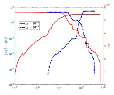
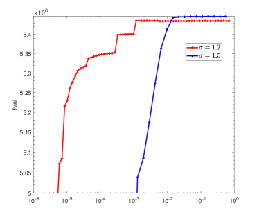
For the implementation of EPalm and EPalmLS, we first take a closer look at the choice of the parameters involved in Algorithm 4.1. The choice of $m$ involves a trade-off between the quality of solutions and the computation cost. A smaller $m$ requires less computation cost but makes subproblem (48) vulnerable to more bad stationary points. To ensure that the solutions returned by Algorithm 4.1 are of high quality, we suggest $m\in[80,120]$ for practical computation, and choose $m=100$ for the all subsequent tests. For the parameter $\rho_{0}$, Figure 1 (a) below shows that the final objective value $\langle\widetilde{C},V^{l_{f}}\rangle$ and penalty term $\|V^{l_{f}}\|_{F}^{2}-\|V^{l_{f}}\|^{2}$ (reflecting the rank of $V^{l_{f}}$) yielded with $\rho_{0}=10^{-8}$ (in red lines) are lower than those yielded with $\rho_{0}=10^{-5}$ (in blue lines); while for the parameter $\sigma$, Figure 1 (b) indicates that the final objective value returned with $\sigma=1.2$ is less than the one returned with $\sigma=1.5$. This shows that smaller $\rho_{0}$ and $\sigma$ lead to a better objective value. As a trade-off between quality of solutions and running time, we choose $\rho_{0}\!=\!10^{-8}$, and $\sigma=1.2$ if $\rho_{l}>10^{-3}$, otherwise $\sigma=1.3$. The other parameters of Algorithm 4.1 are chosen to be as follows:

$$l_{\rm max}=10^{3},\,\rho_{\rm max}=10^{5},\,\epsilon_{1}=\epsilon_{2}=10^{-5},\,\underline{\tau}=10^{-3},\,\underline{\tau}=0.5\ \ {\rm and}\ \ \varsigma=0.9.$$

(a)

(b)

Figure 1: Influence of parameters $\rho_{0}$ and $\sigma$ on the objective value and rank

To capture a high-quality solution, it is reasonable to require the initial $V^{0}\in\mathbb{R}^{m\times p}$ to have a full row rank. This can be easily realized, for example, when $V^{0}$ is generated randomly in MATLAB command ${\rm randn}(m,p)$, by (Vershynin12, , Corollary 5.35) there is a high probability for $V^{0}$ to have a full row rank. For the subsequent testing, we choose $V^{0}$ in terms of MATLAB command $\textrm{randn}(m,p)$ with a fixed seed for all test problems.

For Algorithm 1, we choose $\overline{\beta}=10^{8},\gamma_{\beta}=1.05,\beta_{0}=1$ and $\varepsilon_{k}\equiv 0.9\tau_{l}$. The approximate accuracy $\varepsilon_{k}$ has a difference from that of Algorithm 1 by considering that Algorithm 1 is now seeking $\tau_{l}$-approximate stationary points of a finite number of subproblems (48). During the testing, we terminate Algorithm 1 at the iterate $V^{l,k+1}$ whenever it is such that inclusion (3) holds, and the existence of such an iterate is implied by the proof of Theorem 4.1. We adopt the limited-memory BFGS with the number of memory $l_{m}=15$ and the maximum number of iterates $300$ to seek $V^{l,k,\nu}$ in step 2 of Algorithm A.

For the fairness of numerical comparison, EPalm1 uses the same starting point and parameters as those used by EPalm and EPalmLS. Since the running time of Gurobi would be unacceptable if the known best value is chosen to be its termination criterion, we use the running time required by EPalm as the stopping condition of Gurobi.

5.2 Numerical results for QAPLIB data

We compare the performance of EPalm and EPalmLS with that of EPalm1 and Gurobi for solving problem (1) with $C=0$ and $A,B\in\mathbb{R}^{n\times n}$ from QAPLIB QAPLIB . The total 121 test examples are divided into three groups in terms of size: $n\in\!\{10,\ldots,30\},\{31,\ldots,60\}$, $\{61,\ldots,90\}$. Tables 1-3 report the objective values, relative gaps, and running time (in seconds) of four solvers, where the gap value marked in red means the better one between EPalm and EPalm1. To check whether the three solvers based on global exact penalty could produce $X^{*}$ with desirable approximate feasibility, Tables 1-3 also report infeas of $X^{\rm out}$ corresponding to the output of EPalm. Since the infeasibility of the outputs to EPalmLS and EPalm1 keeps the same magnitude as that of EPalm, we do not report it. Tables 1-3 show that the infeasibility yielded by EPalm is about $10^{-6}$ for all instances.

From Tables 1-3, there are 48 examples for which EPalm yields better objective values than EPalm1, and there are 37 examples for which EPalm yields worse objective values than EPalm1. For the $14$ large-scale test examples, EPalm produces better objective values for 11 ones than EPalm1. In particular, the running time of EPalm is much less than that of EPalm1 for most of exmaples, especially for those of large-size. This validates the superiority of the exact penalty model (1.2) and its factorized formulation.

From Tables 1-3, we see that EPalmLS returns the best objective value for all test instances except “lipa80b” and “lipa90b”, and the running time required by EPalmLS for each instance is comparable with the one required by EPalm. Gurobi and EPalm have similar performance in terms of the number of examples with better objective values. There are 51 examples for which EPalm yields better objective values than Gurobi, and there are 52 examples for which EPalm yields worse objective values than Gurobi. From Table 3, EPalmLS returns the solutions of high quality for the large-scale instance “lipa90a” in $\textbf{6000}s$, and for the most difficult “sko90” in 6.5 hours. It yields the relative gaps not more than $2.87\%$ except for “lipa80b” and “lipa90b”. In addition, we find that the outputs of EPalm, EPalmLS and EPalm1 are rank-one for all test instances though the final penalty factor $\rho$ is generally less than $10^{3}$ for most of test instances. This fully reflects the advantage of the global exact penalty of models (1.2) and (3.3).

Table 1: Numerical results of four solvers on small size QAPLIB instances

No.	Prob.	Optval	EPalm				EPalmLS			EPalm1			Gurobi
			Obj	gap(%)	infeas	time(s)	Obj	gap(%)	time(s)	Obj	gap(%)	time(s)	Obj	gap(%)	time(s)
1	bur26a	5426670	5434878	0.15	4.3e-6	204.2	5426670	0	214.4	5438266	0.21	246.6	5436277	0.18	204.2
2	bur26b	3817852	3821239	0.09	3.7e-8	211.4	3817852	0	212.2	3820388	0.07	235.5	3824753	0.18	211.4
3	bur26c	5426795	5440427	0.25	5.7e-6	215.7	5426795	0	226.5	5429466	0.05	316.3	5430405	0.07	215.7
4	bur26d	3821225	3824565	0.09	4.6e-7	201.0	3821225	0	211.7	3822994	0.05	223.0	3857859	0.96	201.1
5	bur26e	5386879	5391220	0.08	6.5e-8	192.5	5386879	0	203.5	5391811	0.09	289.8	5404115	0.32	192.6
6	bur26f	3782044	3783902	0.05	2.8e-6	206.1	3782044	0	215.8	3785527	0.09	300.5	3801832	0.52	206.2
7	bur26g	10117172	10122238	0.05	3.9e-6	203.2	10117172	0	213.6	10146850	0.29	284.4	10174363	0.57	203.2
8	bur26h	7098658	7106886	0.12	9.1e-8	199.9	7098658	0	211.9	7108689	0.14	225.2	7153958	0.78	199.9
9	chr12a	9552	9552	0	5.7e-6	1.8	9552	0	2.9	9552	0	2.4	9552	0	1.0
10	chr12b	9742	9742	0	5.4e-6	2.2	9742	0	3.6	9742	0	3.4	9742	0	0.5
11	chr12c	11156	11156	0	3.0e-6	2.0	11156	0	3.2	11156	0	4.1	11156	0	2.0
12	chr15a	9896	10010	1.15	2.2e-6	4.5	9896	0	6.5	9896	0	13.1	10638	7.50	4.5
13	chr15b	7990	7990	0	2.4e-6	3.6	7990	0	5.5	7990	0	7.0	7990	0	1.2
14	chr15c	9504	9504	0	3.0e-6	4.1	9504	0	6.2	9504	0	4.6	10802	13.66	4.2
15	chr18a	11098	11098	0	6.4e-6	9.0	11098	0	11.9	11098	0	34.0	14784	33.21	9.0
16	chr18b	1534	1534	0	3.3e-6	7.7	1534	0	10.2	1534	0	17.8	1534	0	1.8
17	chr20a	2192	2196	0.18	3.9e-6	16.6	2192	0	20.0	2196	0.18	45.2	2470	12.68	16.6
18	chr20b	2298	2298	0	4.5e-6	12.3	2298	0	15.4	2298	0	36.0	2570	11.84	12.3
19	chr20c	14142	14146	0.16	5.0e-6	16.1	14142	0	19.9	14160	0.13	25.5	14142	0	9.7
20	chr22a	6156	6184	0.45	2.0e-6	48.8	6156	0	53.4	6184	0.45	97.2	6416	4.22	48.8
21	chr22b	6194	6292	1.58	1.4e-6	47.4	6276	1.32	51.7	6194	0	40.1	6626	6.97	47.5
22	chr25a	3796	3796	0	1.4e-6	40.4	3796	0	45.8	3796	0	73.0	4394	15.75	40.4
23	els19	17212548	17261065	0.28	2.8e-6	14.0	17212548	0	17.9	17388162	1.02	24.3	17212548	0	11.1
24	esc16a	68	68	0	5.5e-6	8.0	68	0	10.3	68	0	10.3	68	0	8.3
25	esc16b	292	296	1.37	4.0e-6	8.3	292	0	10.2	292	0	12.7	292	0	8.4
26	esc16c	160	164	2.50	2.4e-6	13.0	160	0	15.4	168	5.00	14.3	160	0	13.0
27	esc16d	16	16	0	1.4e-7	6.0	16	0	7.7	16	0	8.1	16	0	6.0
28	esc16e	28	28	0	2.7e-6	8.1	28	0	9.6	28	0	7.9	28	0	1.8
29	esc16g	26	28	7.69	3.6e-6	7.6	26	0	9.6	26	0	8.9	26	0	4.4
30	esc16h	996	996	0	5.7e-7	6.0	996	0	7.7	1002	0.60	9.3	996	0	6.0
31	esc16i	14	14	0	4.5e-6	6.4	14	0	8.1	14	0	10.2	14	0	6.4
32	esc16j	8	8	0	3.2e-6	7.5	8	0	9.2	8	0	9.0	8	0	0.3
33	had12	1652	1652	0	3.2e-5	2.8	1652	0	4.2	1652	0	6.3	1652	0	2.8
34	had14	2724	2724	0	2.7e-6	4.5	2724	0	6.8	2724	0	6.2	2730	0.22	4.5
35	had16	3720	3724	0.11	4.9e-5	8.7	3720	0	11.6	3722	0.05	11.8	3746	0.70	8.7
36	had18	5358	5358	0	1.7e-6	21.0	5358	0	24.7	5358	0	24.8	5412	1.01	21.0
37	had20	6922	6922	0	8.1e-6	41.0	6922	0	45.6	6922	0	51.9	6968	0.66	41.0
38	kra30a	88900	93650	5.34	1.7e-6	352.7	89900	1.12	364.8	95060	6.93	344.1	93450	5.12	352.7
39	kra30b	91420	93590	2.37	2.9e-6	333.0	91490	0.08	344.8	93980	2.80	320.1	95950	4.96	333.1
40	lipa20a	3683	3683	0	3.0e-6	21.8	3683	0	25.0	3683	0	12.5	3789	2.88	21.8
41	lipa20b	27076	27076	0	1.2e-6	12.4	27076	0	15.6	27076	0	8.0	27076	0	12.4
42	lipa30a	13178	13455	2.10	3.2e-7	133.7	13178	0	141.6	13442	2.00	106.9	13446	2.03	133.7
43	lipa30b	151426	151426	0	2.1e-6	69.7	151426	0	76.9	151426	0	41.1	151426	0	69.7

Table 1: (continued)

No.	Prob.	Optval	EPalm				EPalmLS			EPalm1			Gurobi
			Obj	gap(%)	infeas	time(s)	Obj	gap(%)	time(s)	Obj	gap(%)	time(s)	Obj	gap(%)	time(s)
44	nug12	578	590	2.08	6.7e-6	4.4	578	0	5.9	590	2.08	5.6	586	1.38	4.5
45	nug14	1014	1018	0.39	3.4e-6	7.8	1014	0	10.1	1018	0.39	8.7	1032	1.78	7.9
46	nug15	1150	1152	0.17	3.6e-6	10.5	1150	0	13.2	1152	0.17	14.3	1160	0.87	10.5
47	nug16a	1610	1610	0	3.3e-6	15.5	1610	0	18.7	1610	0	22.1	1684	4.60	15.5
48	nug16b	1240	1244	0.32	3.9e-6	18.7	1240	0	22.0	1250	0.81	21.8	1282	3.39	18.8
49	nug17	1732	1734	0.12	1.2e-6	27.2	1732	0	31.0	1734	0.12	34.0	1758	1.50	27.2
50	nug18	1930	1944	0.73	5.4e-6	32.7	1930	0	37.0	1960	1.55	38.0	2018	4.56	32.8
51	nug20	2570	2580	0.39	2.4e-6	53.2	2570	0	58.5	2570	0	46.8	2678	4.20	53.2
52	nug21	2438	2512	3.04	5.4e-6	86.3	2438	0	92.5	2452	0.57	89.7	2480	1.72	86.3
53	nug22	3596	3646	1.39	9.4e-8	95.4	3596	0	103.3	3658	1.72	114.6	3620	0.67	95.5
54	nug24	3488	3544	1.61	3.3e-6	108.5	3488	0	117.1	3518	0.86	87.9	3692	5.85	108.5
55	nug25	3744	3796	1.39	4.1e-6	130.2	3744	0	137.6	3756	0.32	116.3	3806	1.66	130.2
56	nug27	5234	5262	0.53	4.9e-6	180.6	5234	0	190.5	5398	3.13	200.1	5394	3.06	180.7
57	nug28	5166	5286	2.32	2.6e-6	201.8	5166	0	212.8	5356	3.68	244.2	5328	3.14	201.8
58	nug30	6124	6296	2.81	2.3e-6	230.2	6134	0.16	242.2	6296	2.81	289.0	6184	0.98	230.2
59	rou12	235528	235852	0.14	1.8e-6	3.0	235528	0	4.4	235654	0.05	4.0	235528	0	3.1
60	rou15	354210	354210	0	3.1e-6	9.1	354210	0	11.4	354211	1.4e-4	12.1	367658	3.80	9.1
61	rou20	725522	736335	1.49	4.2e-6	42.9	726812	0.18	47.3	728812	62.2	48.1	739918	1.98	43.0
62	scr12	31410	31410	0	1.2e-6	3.5	31410	0	5.0	31410	0	4.6	31876	1.48	3.5
63	scr15	51140	51140	0	3.5e-6	6.0	51140	0	8.5	51140	0	8.5	53942	5.48	6.1
64	scr20	110030	110030	0	2.4e-7	62.9	110030	0	68.5	110386	0.32	57.6	119050	8.20	62.9
65	tai10a	135028	135028	0	3.4e-6	2.1	135028	0	2.9	135028	0	2.5	135028	0	2.1
66	tai12a	224416	224416	0	1.1e-5	2.3	224416	0	3.7	224416	0	2.4	234940	4.69	2.3
67	tai12b	39464925	39477067	0.03	4.5e-6	4.8	39464925	0	6.7	39477275	0.03	4.8	40376142	2.31	4.9
68	tai15a	388214	388871	0.17	2.1e-6	8.7	388214	0	11.1	388870	0.17	14.3	400692	3.21	8.8
69	tai15b	51765268	52270480	0.98	2.2e-6	3.5	51765268	0	5.6	52328073	1.09	5.6	51949882	0.36	3.5
70	tai17a	491812	497053	1.07	3.8e-6	23.0	491812	0	26.5	497052	1.07	34.5	507568	3.20	23.0
71	tai20a	703482	731208	3.94	6.7e-6	47.5	710410	0.98	52.4	718063	2.07	37.3	734362	4.39	47.6
72	tai20b	122455319	122455529	1.7e-4	4.9e-6	63.6	122455319	0	69.8	123262175	0.66	67.3	125482444	2.47	63.6
73	tai25a	1167256	1190068	1.95	3.0e-6	80.3	1177820	0.91	86.5	1209934	3.66	62.6	1227678	5.18	80.4
74	tai25b	344355646	351747237	2.15	3.5e-6	231.0	344355646	0	240.3	344904222	0.16	205.2	377247851	9.55	231.1
75	tai30a	1818146	1881406	3.48	5.0e-8	158.6	1848058	1.65	168.6	1877730	3.28	125.6	1903452	4.69	158.6
76	tai30b	637117113	646899645	1.54	2.3e-6	361.7	637808503	0.11	378.2	648008862	1.71	537.3	640779501	0.57	361.7
77	tho30	149936	154166	2.82	2.4e-6	247.2	150216	0.19	260.7	157432	5.00	204.7	157784	5.23	247.3

Table 2: Numerical results of four solvers on medium size QAPLIB instances

No.	Prob.	Optval	EPalm				EPalmLS			EPalm1			Gurobi
			Obj	gap(%)	infeas	time(s)	Obj	gap(%)	time(s)	​Obj	gap(%)	time(s)	Obj	gap(%)	time(s)
78	esc32a	130	154	18.46	2.4e-6	308.1	132	1.54	322.5	144	10.8	267.1	140	7.69	308.1
79	esc32b	168	192	14.29	3.7e-6	396.5	168	0	411.8	192	14.29	320.6	192	14.29	396.6
80	esc32c	642	646	0.62	2.5e-6	438.4	642	0	454.8	662	3.12	500.2	642	0	438.4
81	esc32d	200	208	4.00	5.3e-6	413.1	200	0	426.5	200	0	306.9	200	0	413.1
82	esc32e	2	2	0	3.5e-7	117.5	2	0	123.4	2	0	112.1	2	0	0.4
83	esc32g	6	6	0	3.8e-7	157.6	6	0	164.0	6	0	112.4	6	0	9.0
84	esc32h	438	446	1.83	6.0e-6	429.2	438	0	443.5	452	3.20	454.8	442	0.91	429.2
85	kra32	88700	97580	9.76	2.8e-6	377.7	88700	0	391.2	93200	4.84	398.8	91020	2.62	377.7
86	lipa40a	31538	32100	1.78	1.7e-6	525.4	31900	1.15	543.2	32139	1.91	363.8	32099	1.78	525.5
87	lipa40b	476581	559496	17.40	2.8e-6	526.2	476581	0	575.1	476581	0	177.7	476581	0	526.3
88	lipa50a	62093	63123	1.66	1.0e-7	824.7	62729	1.02	867.2	63228	1.83	3188.0	63041	1.53	824.8
89	lipa50b	1210244	1447039	19.57	1.3e-6	911.4	1210244	0	952.4	1424825	17.73	4311.0	1210244	0	911.7
90	lipa60a	107218	108818	1.49	5.6e-6	1618.4	108140	0.86	1671.8	109055	1.71	8425.2	108553	1.25	1619.0
91	lipa60b	2520135	3046017	20.87	8.1e-8	1352.8	2520135	0	1410.6	3062148	21.51	1323.1	2520135	0	1353.0
92	sko42	15812	16506	4.39	6.3e-6	734.5	15926	0.72	752.6	16742	5.88	514.7	16300	3.09	734.9
93	sko49	23386	24738	5.78	1.2e-7	1562.9	23544	0.68	1597.3	24554	4.99	1080.2	24170	3.35	1563.0
94	sko56	34458	36160	4.94	1.6e-6	2318.6	34688	0.67	2376.5	36286	5.31	2449.8	35802	3.90	2318.8
95	ste36a	9526	10224	7.33	1.5e-6	374.7	9588	0.65	392.9	10176	6.82	723.9	9894	3.86	374.7
96	ste36b	15852	18626	17.50	7.2e-7	219.5	15852	0	235.5	18102	14.19	694.5	17272	8.96	219.5
97	ste36c	8239110	8698706	5.58	2.3e-6	494.2	8301836	0.76	514.9	8797712	6.78	583.6	8695510	5.54	494.2
98	tai35a	2422002	2561206	5.75	4.1e-6	264.6	2468474	1.92	278.9	2539132	4.84	187.2	2551970	5.37	264.6
99	tai35b	283315445	286515255	1.13	1.6e-6	535.4	284003605	0.24	558.1	298665097	5.42	918.7	287507766	1.48	535.4
100	tai40a	3139370	3311302	5.48	2.7e-6	427.9	3197182	1.84	443.7	3241204	3.24	379.9	3334710	6.22	428.0
101	tai40b	637250948	659381790	3.47	2.6e-6	915.4	637409544	0.02	939.1	663614094	4.14	1535.3	687592716	7.90	915.5
102	tai50a	4941410	5279435	6.84	3.2e-6	993.3	5063740	2.48	1034.7	5226263	5.76	842.5	5239852	6.04	993.5
103	tai50b	458821517	481076285	4.85	2.4e-6	2436.0	459222696	0.09	2506.9	499054504	8.77	3375.1	481028897	4.84	2436.2
104	tai60a	7208572	7645348	6.06	2.7e-6	2465.3	7415702	2.87	2546.3	7569875	5.01	1478.0	7694338	6.74	2465.5
105	tai60b	608215054	645761562	6.17	1.2e-6	5096.0	608626078	0.07	5274.5	642247688	5.60	9194.1	634987214	4.40	5096.4
106	tho40	240516	259502	7.89	2.5e-6	911.2	242072	0.65	933.2	264742	10.07	694.4	250554	4.17	911.3
107	wil50	48816	50014	2.45	4.6e-8	1568.1	48938	0.25	1603.9	50058	2.54	1408.3	49952	2.33	1568.2

Table 3: Numerical results of four solvers on large size QAPLIB instances

No.	Prob.	Optval	EPalm				EPalmLS			EPalm1			Gurobi
			Obj	gap(%)	infeas	time(s)	Obj	gap(%)	time(s)	Obj	gap(%)	time(s)	Obj	gap(%)	time(s)
108	esc64a	116	124	6.90	2.5e-6	9412.1	116	0	9433.1	130	12.07	9658.1	116	0	9412.4
109	lipa70a	169755	172255	1.47	4.3e-6	2675.0	171080	0.78	2769.9	172751	1.76	16998.0	171756	1.18	2675.7
110	lipa70b	4603200	5632370	22.36	1.7e-6	3516.4	4603200	0	3610.2	5684608	23.49	11686.1	4603200	0	3516.8
111	lipa80a	253195	256760	1.41	1.8e-6	4723.5	255007	0.72	4840.7	257586	1.73	31206.5	255853	1.05	4724.5
112	lipa80b	7763962	9551075	23.02	2.8e-7	3597.3	9356211	20.51	3734.1	9619503	23.90	20113.6	7763962	0	3599.4
113	lipa90a	360630	365304	1.30	8.2e-7	5717.1	363000	0.66	5959.4	366463	1.62	58404.8	364155	0.98	5718.6
114	lipa90b	12490441	15424375	23.49	2.0e-6	11432.7	14688281	17.60	11634.6	15535319	24.38	40583.2	12490441	0	11434.4
115	sko64	48498	51146	5.46	1.1e-6	6191.6	48800	0.62	6392.8	51124	5.41	8722.1	49912	2.92	6191.9
116	sko72	66256	70558	6.49	1.2e-6	8971.4	66834	0.87	9346.4	70322	6.14	16671.3	68240	2.99	8972.3
117	sko81	90998	95696	5.16	6.7e-6	20472.2	91636	0.70	21281.1	95908	5.40	25397.3	93344	2.58	20472.8
118	sko90	115534	122184	5.76	3.4e-6	14925.4	116494	0.83	15825.4	122608	6.12	53349.2	118558	2.62	14926.0
119	tai64c	1855928	1979532	6.66	2.1e-6	4827.8	1855928	0	4945.8	1856396	0.03	3763.4	1866152	0.55	4828.0
120	tai80a	13557864	14386541	6.11	3.2e-6	7489.4	13868148	2.29	7653.6	14399934	6.21	15206.7	14216380	4.86	7491.0
121	tai80b	818415043	883500297	7.95	1.3e-6	20262.4	823115708	0.57	20569.4	911680600	11.40	38052.7	866360822	5.86	20262.9

Table 4 reports the number of instances computed with four solvers within seven relative gap levels. EPalmLS yields the best relative gaps and returns the relative gaps less than $5.0\%$ for 119 instances. EPalm is a little worse than EPalm1 in terms of the relative gaps, and it is superior to Gurobi in terms of the number of instances with relative gaps less than $1.0\%$, and is worse than Gurobi in terms of the number of instances with relative gaps more than $5.0\%$. In addition, EPalm is superior to Gurobi for instances of small-size, but has a worse performance than Gurobi for those of medium and large-size.

Table 4: The gap levels of four solvers for the 121 QAPLIB instances

	Gap$\leq$%	0.0	0.5	1.0	5.0	10.0	20.0	$>20$
	EPalm	34	55	57	92	112	117	4
Total	EPalmLS	82	91	109	119	119	120	1
	EPalm1	40	59	65	96	110	117	4
	Gurobi	32	39	53	97	115	120	1
	EPalm	32	52	54	75	77	77	0
small-size	EPalmLS	67	72	74	77	77	77	0
	EPalm1	35	54	60	76	77	77	0
	Gurobi	21	28	38	63	72	76	1
	EPalm	2	2	3	14	24	29	1
medium-size	EPalmLS	12	16	24	30	30	30	0
	EPalm1	4	4	4	16	24	29	1
	Gurobi	7	7	8	21	29	30	0
	EPalm	0	0	0	3	11	11	3
large-size	EPalmLS	3	3	11	12	12	13	1
	EPalm1	1	1	1	4	9	11	3
	Gurobi	4	4	7	13	14	14	0

We also compare the objective values returned by EPalm and EPalmLS with the upper bounds yielded by rPRSM of Graham22 . For the 75 test instances listed in (Graham22, , Tables 1-3), EPalm yields the better upper bounds than rPRSM for 43 instances, and the worse upper bounds for 19 instances; while EPalmLS produces the better upper bounds for 54 instances, and the worse upper bound only for one instance.

5.3 Numerical results for Dre problems

As described in Drezner05 , the ‘dre’ test instances are based on a rectangular grid where all nonadjacent nodes have zero weight. This way, a pair exchange of the optimal permutation will result in many adjacent pairs becoming non-adjacent, which making the value of the objective function will increase quite steeply. The ‘dre’ instances are difficult to solve, especially for many metaheuristic-based methods because they are ill-conditioned and hard to break out the ‘basin’ of the local minimal. These instances are available in http://business.fullerton.edu/zdrezner, and the best known solutions have been found by branch and bound in Drezner05 .

Table 5 reports the results of four solvers to compute the ‘dre’ test instances. For the 10 test instances, EPalm and EPalmLS produce the best objective values for 7 instances, EPalm1 yields the best ones for 6 instances, and Gurobi returns the best ones only for 3 intances. For the last three instances, EPalmLS still returns the lower relative gaps than EPalm and EPalm1, and has better performance than Gurobi except for “dre90”; while EPalm returns lower relative gaps than EPalm1 and Gurobi only for “dre72”.

Table 5: Numerical results of four solvers on ’dre’ instances

No.	Prob.	Optval	EPalm				EPalmLS			EPalm1			Gurobi
			Obj	gap(%)	infeas	time(s)	Obj	gap(%)	time(s)	Obj	gap(%)	time(s)	Obj	gap(%)	time(s)
1	dre15	306	306	0	3.9e-6	5.0	306	0	9.2	306	0	7.8	306	0	2.6
2	dre18	332	332	0	2.2e-5	11.9	332	0	19.1	332	0	18.4	332	0	8.0
3	dre21	356	356	0	2.6e-6	18.1	356	0	31.0	356	0	85.0	356	0	10.4
4	dre24	396	396	0	4.0e-6	36.2	396	0	67.7	396	0	100.6	538	35.86	36.3
5	dre28	476	476	0	1.0e-6	93.0	476	0	157.6	476	0	180.0	792	66.39	93.0
6	dre30	508	508	0	2.0e-6	103.0	508	0	185.5	508	0	196.0	826	62.60	103.1
7	dre42	764	764	0	3.6e-6	725.1	764	0	770.5	1244	62.83	857.9	1294	69.37	725.1
8	dre56	1086	1974	81.77	3.8e-6	5013.6	1726	58.93	5219.7	1920	76.80	5548.0	1888	73.85	5013.7
9	dre72	1452	2762	90.22	7.8e-7	12320.9	2604	79.34	12430.4	2800	92.84	8291.4	2792	92.29	12321.3
10	dre90	1838	4372	137.87	3.9e-6	52063.7	3518	91.40	52659.0	4210	129.05	45976.8	3440	87.16	52064.6

6 Conclusion

We presented an equivalent rank-one DNN reformulation (1.2) with fewer equality constraints for the QAP, and established three kinds of local error bounds for its feasible set $\Gamma$. With the help of these error bounds, we confirmed that problems (1.2) and (1.2) are respectively the global exact penalty of (1.2) and (1.2), while problems (1.1) and (3.3) are the global exact penalty of (1.1) and (46), respectively. The latter not only removes the restricted assumption required by the conclusion of Jiang21 , but also supplements the global exact penalty result for its BM factorization. A continuous relaxation approach was developed by applying the ALM to seek approximate stationary points of a finite number of exact penalty problems (1.2) with increasing $\rho$, and the asymptotic convergence analysis of the ALM was also established under a mild condition. Extensive numerical tests validate the advantage of the rank-one DNN reformulation (1.2) over the one used in Jiang21 , and numerical comparison shows that EPalm has a comparable performance with Gurobi in terms of the quality of solutions, while its local-search version EPalmLS is significantly superior to Gurobi in terms of the quality of solutions.

Conflict of interest

The authors declare that they have no conflict of interest.

References

- (1) W. P. Adams, M. Guignard, P. M. Hahn and W. L. Hightower, linearization technique bound for the quadratic assignment problem, European Journal of Operations Research, 180, 983-996 (2007).
- (2) K. Anstreicher and H. Wolkowicz, On Lagrangian relaxation of quadratic matrix constraints, SIAM Journal on Matrix Analysis and Applications, 22, 41-55 (2000).
- (3) K. Bai, J. J. Ye and J. Zhang, Directional quasi-/pseudo-normality as sufficient conditions for metric subregularity, SIAM Journal on Optimization, 29, 2625-2649 (2019).
- (4) S. Burer, R. D. C. Monteiro and Y. Zhang, Rank-two relaxation heuristics for max-cut and other binary quadratic programs, SIAM Journal on Optimization, 12, 503-521 (2001).
- (5) S. Burer and R. D. C. Monteiro, A nonlinear programming algorithm for solving semidefinite programs via low-rank factorization, Mathematical Programming, 95, 329-357 (2003).
- (6) R. Burkard, E. Cela and B. Klinz, On the biquadratic assignment problem, In Quadratic Assignment and Related Problems, DIMACS Series in Discrete Mathematics and Theoretical Computer Science, American Mathematical Society, 16, 117-146 (1994).
- (7) R. Burkard, Quadratic assignment problems, in Handbook of Combinatorial Optimization, P. M. Pardalos, D. Z. Du, and R. L. Graham, eds., 2741-2814, Springer, New York, 2013.
- (8) F. H. Clarke, Optimization and Nonsmooth Analysis, New York, 1983.
- (9) P. Z. Chinn, J. Chvatalova, A. K. Dewdney, and N. E. Gibbs, The bandwidth problem for graphs and matrices-a survey, Journal of Graph Theory, 6, 223-254 (1982).
- (10) D. Conte, P. Foggia, C. Sansone and M. Vento, Thirty years of graph matching in pattern recognition, International Journal of Pattern Recognition Artificial Intelligence, 18, 265-298 (2004).
- (11) A. L. Dontchev and R. T. Rockafellar, Implicit Functions and Solution Mappings, Springer Monographs in Mathematics, LLC, New York, 2009.
- (12) Z. Drezner, P. Hahn and E. D. Taillard, Recent advances for the quadratic assignment problem with special emphasis on instances that are difficult for meta-heuristic methods, Annals of Operations Research, 139, 65-94 (2005).
- (13) Z. Drezner, The quadratic assignment problem, in Location Science, 345-363, Springer, New York, 2015.
- (14) M. Fischetti, M. Monaci and D. Salvagnin, Three ideas for the quadratic assignment problem, Operations Research, 60, 954-964 (2012).
- (15) H. Gfrerer, First order and second order characterizations of metric subregularity and calmness of constraint set mappings, SIAM Journal on Optimization, 21, 1439-1474 (2011).
- (16) N. Graham, H. Hu, J. Y. Im, X. X. Li and H. Wolkowicz, A restricted dual Peaceman-Rachford splitting method for a strengthened DNN relaxation for QAP, Informs Journal on Computing, 34, 2125-2143 (2023).
- (17) R. Henrion and J. Outrata, Calmness of constraint systems with applications, Mathematical Programming, 104, 437-464 (2005).
- (18) R. A. Horn and C. R. Johnson, Matrix analysis, Cambridge, U.K.: Cambridge University Press, 1987.
- (19) A. D. Ioffe, Regular points of Lipschitz functions, Transactions of the American Mathematical Society, 251, 61-69 (1979).
- (20) A. D. Ioffe and J. V. Outrata, On metric and calmness qualification conditions in subdifferential calculus, Set-Valued Analysis, 16, 199-227 (2008).
- (21) X. X. Jia, C. Kanzow, P. Mehlitz and G. Wachsmuth, An augmented Lagrangian method for optimization problems with structured geometric constraints, Mathematical Programming, 199, 1365-1415 (2023).
- (22) B. Jiang, Y. F. Liu and Z. W. Wen, -norm regularization algorithms for optimization over permutation matrices, SIAM Journal on Optimization, 26, 2284-2313 (2016).
- (23) B. Jiang, X. Meng, Z. W. Wen and X. J. Chen, An exact penalty approach for optimization with nonnegative orthogonality constraints, Mathematical Programming, 198, 855–897 (2022).
- (24) Z. X. Jiang, X. Y. Zhao and C. Ding, A proximal DC approach for quadratic assignment problem, Computational Optimization and Applications, 78, 825–851 (2021).
- (25) E. De Klerk and D. V. Pasechnik, Approximation of the stability number of a graph via copositive programming, SIAM Journal on Optimization, 12, 875-892 (2002).
- (26) S. Y. Kim, M. Kojima and K. C. Toh, A Lagrangian–DNN relaxation: a fast method for computing tight lower bounds for a class of quadratic optimization problems, Mathematical Programming, 156, 161-187 (2016).
- (27) Y. L. Lai and K. Williams, A survey of solved problems and applications on bandwidth, edgesum, and profile of graphs, Journal of Graph Theory, 31, 75-94 (1999).
- (28) E. L. Lawler, The quadratic assignment problem, Management Science, 9, 586-599 (1963).
- (29) C. P. Lee, L. Liang, T. Y. Tang and K. C. Toh, Accelerating nuclear-norm regularized low-rank matrix optimization through Burer-Monteiro decomposition, arXiv:2204.14067v2, 2023.
- (30) A. S. Lewis, The convex analysis of unitarily invariant matrix functions, Journal of Convex Analysis, 2, 173–183 (1995).
- (31) Y. L. Liu, S. J. Bi and S. H. Pan, Equivalent Lipschitz surrogates for zero-norm and rank optimization problems, Journal of Global Optimization, 72, 679-704 (2018).
- (32) D. C. Liu and J. Nocedal, On the limited memory BFGS method for large scale optimization, Mathematical Programming, 45, 503-528 (1989).
- (33) Z. Y. Liu, H. Qiao and L. Xu, An extended path following algorithm for graph-matching problem, IEEE Transactions on Pattern Analysis and Machine Intelligence, 34, 1451-1456 (2012).
- (34) M. Mehlitz, Asymptotic stationarity and regularity for nonsmooth optimization problems, Journal of Nonsmooth Analysis and Optimization, 1, 6575 (2020).
- (35) D. Oliveira, H. Wolkowicz and Y. Xu, ADMM for the SDP relaxation of the QAP, Mathematical Programming Computation, 10, 631-658 (2018).
- (36) L. Pardalos and M. Resende, A greedy randomized adaptive search procedure for the quadratic assignment problem, in Quadratic Assignment and Related Problems, DIMACS Series in Discrete Mathematics and Theoretical Computer Science, American Mathematical Society, 16, 237-261 (1994).
- (37) P. A. Parrilo, Structured semidefinite programs and semialgebraic geometry methods in robustness and optimization, Ph.D. Thesis, California Institute of Technology, Pasadena, 2000.
- (38) J. Povh and F. Rendl, Copositive and semidefinite relaxations of the quadratic assignment problem, Discrete Optimization, 6, 231-241 (2009).
- (39) P. Hahn and M. Anjos, QAPLIB–a quadratic assignment problem library, http://www.seas.upenn.edu/qaplib.
- (40) Y. T. Qian, S. H. Pan and Y. L. Liu, Calmness of partial perturbation to composite rank constraint systems and its applications, Journal of Global Optimization, 85, 867–889 (2023).
- (41) Y. T. Qian, S. H. Pan and L. H. Xiao, Error bound and exact penalty method for optimization problems with nonnegative orthogonal constraint, IMA Journal of Numerical Analysis, https://doi.org/10.1093/imanum/drac084.
- (42) S. M. Robinson, Some continuity properties of polyhedral multifunctions, Mathematical Programming Study, 14, 206-214 (1981).
- (43) R. T. Rockafellar and R. J-B. Wets, Variational Analysis, Springer, 1998.
- (44) A. Silva, L. C. Coelho and M. Darvish, Quadratic assignment problem variants: A survey and an effective parallel memetic iterated tabu search, European Journal of Operations Research, 292, 1066-1084 (2021).
- (45) T. Stutzle, Iterated local search for the quadratic assignment problem, European Journal of Operations Research, 174, 1519–1539 (2006).
- (46) E. Taillard, Robust taboo search for the quadratic assignment problem, Parallel Computing, 17, 443-455 (1991).
- (47) T. Y. Tang and K. C. Toh, Solving graph equipartition SDPs on an algebraic variety, Mathematical Programming, 2023, https://doi.org/10.1007/s10107-023-01952-6.
- (48) T. Tao, Y. T. Qian and S. H. Pan, Column -norm regularized factorization model of low-rank matrix recovery and its computation, SIAM Journal on Optimization, 32, 959-988 (2022).
- (49) R. Vershynin, Introduction to the Non-Asymptotic Analysis of Random Matrices, Cambridge University Press, 2012.
- (50) Z. W. Wen and W. T. Yin, A feasible method for optimization with orthogonality constraints, Mathematical Programming, 142, 397-434 (2013).
- (51) Y. Xia, An efficient continuation method for quadratic assignment problems, Computer & Operations Research, 37, 1027-1032 (2010).
- (52) J. J. Ye and D. L. Zhu, Optimality conditions for bilevel programming problems, Optimization, 33, 9-27 (1995).
- (53) J. J. Ye, D. L. Zhu and Q. J. Zhu, Exact penalization and necessary optimality conditions for generalized bilevel programming problems, SIAM Journal on Optimization, 7, 481-507 (1997).
- (54) J. J. Ye and X. Y. Ye, Necessary optimality conditions for optimization problems with variational inequality constraints, Mathematics of Operations Research, 4, 977-997 (1997).
- (55) M. Zaslavskiy, F. Bach, and J.-P. Vert, A path following algorithm for the graph matching problem, IEEE Transactions on Pattern Analysis and Machine Intelligence, 31, 2227-2242 (2009).
- (56) X. Y. Zheng and K. F. Ng, Metric subregularity and calmness for nonconvex generalized equations in Banach spaces, SIAM Journal on Optimization, 20, 2119-2136 (2010).