Continuous Jumping of a Parallel Wire-Driven Monopedal Robot RAMIEL Using Reinforcement Learning

Abstract

We have developed a parallel wire-driven monopedal robot, RAMIEL, which has both speed and power due to the parallel wire mechanism and a long acceleration distance. RAMIEL is capable of jumping high and continuously, and so has high performance in traveling. On the other hand, one of the drawbacks of a minimal parallel wire-driven robot without joint encoders is that the current joint velocities estimated from the wire lengths oscillate due to the elongation of the wires, making the values unreliable. Therefore, despite its high performance, the control of the robot is unstable, and in 10 out of 16 jumps, the robot could only jump up to two times continuously. In this study, we propose a method to realize a continuous jumping motion by reinforcement learning in simulation, and its application to the actual robot. Because the joint velocities oscillate with the elongation of the wires, they are not used directly, but instead are inferred from the time series of joint angles. At the same time, noise that imitates the vibration caused by the elongation of the wires is added for transfer to the actual robot. The results show that the system can be applied to the actual robot RAMIEL as well as to the stable continuous jumping motion in simulation.

I INTRODUCTION

Legged robots have higher running performance than wheeled robots, among which robots that can traverse three-dimensional uneven terrain by jumping have been developed [1, 2, 3, 4, 5]. While some robots can make a single jump of about 3 m, continuous jumping is difficult because the actuators required for posture control are reduced [4, 5] (note that in this study, the jump height is defined as the maximum difference between the center of gravity height at takeoff and when jumping). On the other hand, robots such as [1, 2, 3] can jump continuously, but these robots have a maximum jump height of about 1.1 m [1], which is inferior to robots with a single jump. Therefore, we have developed a parallel wire-driven monopedal robot RAMIEL (paRAllel wire-driven Monopedal agIlE Leg) that is capable of high and continuous jumps [6] (Fig. 1). By taking advantage of the linear motion of the actuator in the wire-driven robot, RAMIEL has high-speed, high-power linear motion capability and long acceleration distance, ensuring its jumping performance. In previous experiments, RAMIEL has succeeded in a high jump of 1.6 m and a maximum of eight consecutive jumps.

However, its performance is not yet ideal, especially for the continuous jump. This is due to a problem unique to the minimal parallel wire-driven robot. In order to keep the joint structure simple and lightweight, the robot does not have a joint encoder, and the joint angle is estimated from the wire length through Extended Kalman Filter [7]. However, since the wire has some elasticity and stretches, the wire length often oscillates in tasks that require large force such as jumping, and as a result, the estimated joint angle often oscillates. Therefore, when a general controller [8] is applied to RAMIEL, the jumping motion is unstable, and 10 out of 16 trials resulted in less than two consecutive jumps [6].

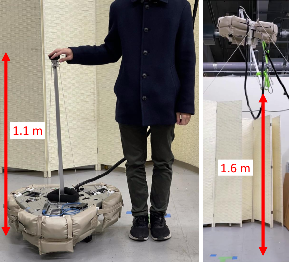
Figure 1: Parallel wire-driven monopedal robot RAMIEL [6].

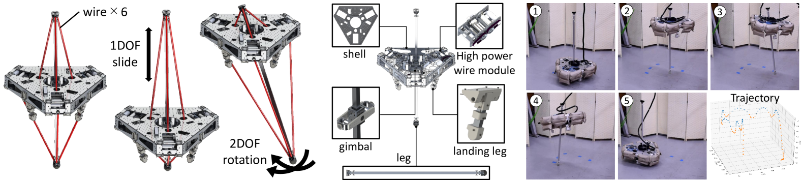
Figure 2: Detailed body structure and performance of continuous jumping of RAMIEL.

Therefore, the objective of this study is to develop a stable continuous jumping motion by reinforcement learning in simulation and transfer it to the actual robot. Various reinforcement learning methods have been developed for learning dynamic behaviors of robots [9, 10, 11, 12, 13]. Some of them have been applied not only to simulations but also to actual robots [10, 11]. Reinforcement learning has also been introduced to some wire-driven robots [12, 13, 14]. On the other hand, [12, 14] is applied only to simulations, and [13] deals only with a simple and relatively static motion of walking with a fixed upper end. In this study, we use reinforcement learning to realize dynamic and difficult jumping motions in a wire-driven robot in simulation and on the actual robot, which are more difficult than those in previous studies on manipulators, quadruped robots, etc. We show how this can be done by sharing know-how such as the design of the reward function for jumping, the state design without using the velocity term (which is vulnerable to noise due to vibration), the method of adding noise, and the system configuration for application to the actual robot. Experimental results show that the simulation results are more stable than those of an existing method, and that our method is applicable to actual robots. We believe that this study is an example of the realization of dynamic motion using reinforcement learning in a wire-driven robot with wire stretching, and that future robot configurations with both speed and power will be developed by taking advantage of the wire-driven robot.

II Parallel Wire-Driven Monopedal Robot RAMIEL

We describe the body configuration and performance of the parallel wire-driven monopedal robot RAMIEL [6] handled in this study. An overview is shown in Fig. 2.

II-A Structure of RAMIEL

II-A1 Body Configuration of RAMIEL

RAMIEL has an overall height of 1.07 m, an overall width of 0.55 m, and a weight of 10.3 kg. The body is mainly divided into the main body and the leg. The leg is made only of aluminum square pipes, fixed wire parts, and rubber parts at the ground contact points, and is very light at 0.5 kg. This makes the leg highly controllable and suppresses impact when landing. The main body has a high-power wire module to control the wires (to be explained later), and landing legs with built-in springs to soften the impact at the time of landing. Between the main body and the landing legs, the robot has a gimbal mechanism with two degrees of freedom (DOFs) of rotation (roll and pitch) and one DOF of linear motion, for a total of three DOFs. The main body is surrounded by a shock-absorbing exterior with an air damper.

II-A2 High-Power Wire Module

RAMIEL is an antagonistic wire-driven robot that drives 3-DOF joints by winding 6 wires. The motor is a Maxon BLDC EC-4pole 200W motor, which is decelerated by a belt at a reduction ratio of 2.5:1 to provide sufficient force and speed. The motor is driven by a motor driver that can operate at an input voltage of 70V and a maximum instantaneous current of 50A [15]. Therefore, a high speed and high torque with a maximum tension of 230 N and a maximum wire winding speed of 10.7 m/sec can be realized, and at the same time, the low gear ratio ensures backdrivability and can cope with impact at landing. This output ideally corresponds to a jump height of about 5.8 m. In addition, the wires are aligned and wound on the pulleys by the level winder mechanism and the wire holding mechanism, which prevents the wires from overlapping on the pulleys and ensures accurate measurement of wire length and wire tension.

II-B Performance of RAMIEL

In [6], the motion control of the jumping is performed by a controller similar to that used in [8]. The motion during jumping is divided into two phases: the stance phase in which the landing legs are on the ground, and the flight phase. In the stance phase, the two rotational DOFs are controlled so that the body posture becomes horizontal, and the linear DOF is controlled by the energy shaping control law so that the target energy is satisfied. In the flight phase, the linear DOF is kept at a certain position, and the two rotational DOFs are controlled by determining the landing point of the target leg based on the horizontal velocity of the robot.

In addition to the 1.6 m jump shown in Fig. 1, the robot has successfully made up to 8 consecutive jumps as shown in the right figure of Fig. 2 with this control law. On the other hand, 10 out of 16 trials resulted in less than two consecutive jumps, which is not a high success rate. The wires used to drive the robot in this study are made of a chemical fiber called Zylon^®. Zylon^® has high tensile strength, but it also has some elasticity and can stretch by up to 2.5%. In addition, the wire can transmit force only in the tensile direction, and when force is applied in the opposite direction, the tension instantly decreases to zero and the wire loosens, which causes vibration. Therefore, sensor values and state estimation are prone to oscillation, which is considered to be the cause of instability in control.

III Continuous Jumping Motion of RAMIEL Using Reinforcement Learning

The overall system configuration and the definitions of action, state, and reward in reinforcement learning are described in this section.

III-A System Architecture

The system configuration of this study is shown in Fig. 3. First, the simulation is conducted using Mujoco [16]. Reinforcement learning is performed using the Proximal Policy Optimization (PPO) [9] of Stable Baselines3 [17]. Here, the simulations show that the body velocity $\bm{\dot{p}}$ ($\in R^{3}$), body rotation matrix $\bm{R}$ ($\in R^{3\times 3}$), body angular velocity $\bm{\omega}$ ($\in R^{3}$), joint angle $\bm{q}$ ($\in R^{3}$), and joint velocity $\bm{\dot{q}}$ ($\in R^{3}$) are obtained as the states. We also compute the reward $\bm{r}$. The action in reinforcement learning is the target joint torque $\bm{\tau}^{ref}$ ($\in R^{3}$). This is converted to the target wire tension $\bm{f}^{ref}$ ($\in R^{6}$) by Action Converter of Section III-B and sent to the robot.

On the other hand, in the actual robot, the PyTorch model obtained from Stable Baselines3 is converted for C++, and only inference is performed using LibTorch. The wire length $\bm{l}$ ($\in R^{6}$) and the wire velocity $\bm{\dot{l}}$ ($\in R^{6}$) are obtained from the motor encoder. In addition, the body acceleration $\bm{\ddot{p}}$ ($\in R^{3}$) and the body angular velocity $\bm{\omega}$ ($\in R^{3}$) are obtained from the inertial sensor, and the body velocity $\bm{\dot{p}}$ ($\in R^{3}$) is obtained from Realsense T265 which performs visual odometry. These are converted by State Converter of Section III-C into $\{\bm{\dot{p}},\bm{R},\bm{\omega},\bm{q},\bm{\dot{q}}\}$ which are the same state inputs as in the simulation. From these, $\bm{\tau}^{ref}$ is calculated using the trained model and converted to $\bm{f}^{ref}$ by Action Converter exactly as in the simulation, and used as the control input to the motor driver. The $\bm{f}^{ref}$ is converted to current and the motor is driven by current control. Since this is a quasi direct-drive mechanism, it is possible to achieve the target tension precisely.

The actual behavior $\bm{a}$ output by the reinforcement learning model is not the direct output of $\bm{\tau}^{ref}$, but the converted value within the range of $[-1,1]$. In other words, when the minimum and maximum values of $\bm{\tau}$ are $\bm{\tau}^{\{min,max\}}$, $\tau^{ref}=\tau^{min}+(\tau^{max}-\tau^{min})(a+1)/2$ for each joint axis. The state $\bm{s}$ actually input to the reinforcement learning model is obtained by processing $\{\bm{\dot{p}},\bm{R},\bm{\omega},\bm{q},\bm{\dot{q}}\}$, which is described in Section III-C. In this study, $\bm{\tau}^{min}=\{-50,-50,-320\}$, $\bm{\tau}^{max}=\{50,50,90\}$ (referring to roll, pitch and linear DOFs in that order). Note that this control loop is executed at 100 Hz.

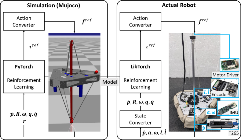
Figure 3: System architecture of reinforcement learning for simulation and the actual robot of RAMIEL.

III-B Definition of Action

In this study, although the control input of the actual robot is the wire tension $\bm{f}^{ref}$, $\bm{f}^{ref}$ is not used as the direct control input because of the increase in learning time due to the increase of search range and the increase in internal force by wire antagonism. Instead, the joint torque $\bm{\tau}^{ref}$ is used as the control input in reinforcement learning, and $\bm{\tau}^{ref}$ is converted to $\bm{f}^{ref}$ in exactly the same way in simulation and in the actual robot (Action Converter). By solving the following quadratic programming, we calculate $\bm{f}^{ref}$ that satisfies $\bm{\tau}^{ref}$ while minimizing the internal forces:

$$\underset{\bm{f}^{ref}}{\textrm{minimize}} \;\;\;\;\;\;\;\;\;\;\;\;\;\;\;\;\;\;\;||\bm{f}^{ref}||^{2}$$ (1)

subject to $$\;\;\;\;\;\;\;\;\;\;\;\;\bm{\tau}^{ref}=-G^{T}(\bm{q})\bm{f}^{ref}$$

$$\;\;\;\;\;\;\;\;\;\;\;\;\bm{f}^{ref}\geq\bm{f}^{min}$$

where $\bm{G}$ is the muscle Jacobian of the wire at the joint angle $\bm{q}$ (which can be calculated from the geometric model), $\bm{f}^{min}$ is the minimum muscle tension, and $||\cdot||$ is the L2 norm. In this study, we set $\bm{f}^{min}=8$ [N].

III-C Definition of State

We convert $\{\bm{\dot{p}},\bm{\ddot{p}},\bm{\omega},\bm{l},\bm{\dot{l}}\}$ obtained in the actual robot to the same $\{\bm{\dot{p}},\bm{R},\bm{\omega},\bm{q},\bm{\dot{q}}\}$ as in the simulation (State Converter). First, by using $\bm{\ddot{p}}$ and $\bm{\omega}$ obtained from IMU, the rotation matrix $\bm{R}$ of the main body is calculated by Madgwick Filter [18]. Next, since the joint angles $\bm{q}$ and joint velocities $\bm{\dot{q}}$ of the actual robot cannot be obtained directly, we estimate them from $\bm{l}$ and $\bm{\dot{l}}$. The following Extended Kalman Filter (EKF) is performed with Eq. 2 as the prediction function and Eq. 3 as the observation function:

$$\bm{x}_{t+1} =\begin{pmatrix}\bm{I}&\bm{I}dt\\ \bm{O}&\bm{I}\end{pmatrix}\bm{x}_{t}+\bm{w}$$ (2)

$$\bm{y}_{t+1} =\bm{h}(\bm{x}_{t})+\bm{v}$$ (3)

$$\bm{h}(\bm{x}_{t}) =\begin{pmatrix}\bm{g}(\bm{q}_{t})\\ \bm{G}(\bm{q}_{t})\bm{\dot{q}}_{t}\end{pmatrix},\bm{x}=\begin{pmatrix}\bm{q}\\ \bm{\dot{q}}\end{pmatrix},\bm{y}=\begin{pmatrix}\bm{l}\\ \bm{\dot{l}}\end{pmatrix}$$

where $\bm{I}$ is the identity matrix, $\bm{O}$ is the zero matrix, $\{\bm{w},\bm{v}\}$ is the Gaussian noise, and $\bm{g}(\bm{q})$ is the wire length at the joint angle $\bm{q}$ ($\bm{G}(\bm{q})$ is its derivative).

We construct the state input $\bm{s}$ for reinforcement learning using $\{\bm{\dot{p}},\bm{R},\bm{\omega},\bm{q},\bm{\dot{q}}\}$ obtained so far. First, the simplest configuration is the one in which $\{\bm{\dot{p}}_{t},\bm{R}^{quat}_{t},\bm{\omega}_{t},\bm{q}_{t},\bm{\dot{q}}_{t}\}$ are the state values (Ours-1). Note that $\bm{R}^{quat}$ is the value obtained by transforming the rotation matrix $\bm{R}$ into quaternion ($\in R^{4}$). Next, we construct a state value that takes into account the problem of this study, i.e., the oscillation of the wire length due to its stretching or loosening, and the resulting oscillation of the joint angle estimation (Ours-2). We use the characteristics that $\bm{q}$ is less sensitive to the vibration than $\bm{\dot{q}}$. Instead of using $\dot{\bm{q}}$ directly, we set $N_{prev}$, which indicates how many previous time steps to be given, and use $\bm{q}$ of the previous steps as the state value. That is, instead of $\dot{\bm{q}}_{t}$, we use $\{\bm{q}_{t-1},\bm{q}_{t-2},\cdots,\bm{q}_{t-N_{prev}}\}$ as state values. In addition to these state values, both Ours-1 and Ours-2 use $\{\bm{\tau}^{ref}_{t-1},\bm{\tau}^{ref}_{t-2},\cdots,\bm{\tau}^{ref}_{t-N_{prev}}\}$ as the state value. Note that we set $N_{prev}=6$ in this study. Ours-1 and Ours-2 are compared in the experiment.

III-D Definition of Reward

In this study, we design the following rewards to generate jumping behaviors. First, the following reward $r_{jump}$ is given for the height of the body in order to generate continuous jumps from the landing state:

$$r_{jump}=\begin{cases}-1&(p_{z}>1.1)\\ p^{2}_{z}&(otherwise)\end{cases}$$ (4)

where $p_{z}$ is the height of the body. The reward is proportional to the square of the height of the body, and at the same time, a penalty is given when the height exceeds 1.1 m in order to prevent jumping too high. Although $\bm{p}_{z}$ is obtained from Realsense T265, we do not use it as a state value because it may be significantly off due to noise.

Next, the following reward $r_{keep}$ is given to the translational velocity of the body in the $xy$ direction and the rotational velocity around the $z$-axis, so that the body makes a jump in-situ:

$$r_{keep}=-c(\dot{p}^{2}_{x}+\dot{p}^{2}_{y}+\omega^{2}_{z})$$ (5)

Note that $c$ is a variable that monotonically increases from 0 to 1 according to the process of learning.

Next, the following reward $r_{horizon}$ is given to keep the body and the leg horizontal and suppress tilting:

$$r_{horizon}=-(1.0-(\bm{R}\cdot\bm{e}_{z})\cdot\bm{e}_{z})-(1.0-(\bm{R}_{leg}\cdot\bm{e}_{z})\cdot\bm{e}_{z})$$ (6)

where $\bm{R}_{leg}$ is the rotation matrix of the leg in the world coordinate and $\bm{e}_{z}=\begin{pmatrix}0&0&1\end{pmatrix}^{T}$. Each for the body and leg, the current vector along the $z$-axis ($\bm{R}\cdot\bm{e}_{z}$) is taken, and the degree of tilt is calculated from the inner product of this vector and the $z$-axis in the world coordinate. When both the body and leg are horizontal, $r_{horizon}$ is zero, and the value increases negatively with the degree of tilt.

Next, the following reward $r_{ctrl}$ is given in order to suppress the increase of control input:

$$r_{ctrl}=-||\bm{w}_{a}\cdot\bm{a}||^{2}$$ (7)

where $\bm{w}_{a}=\begin{pmatrix}3.0&3.0&0.3\end{pmatrix}^{T}$. Since a large force is required in the $z$ direction, the weight for the slide joint is set to be small.

Next, the following reward $r_{contact}$ is given, which reduces the time when the leg and the landing legs of the body make contact with the floor, so that the leg is correctly lifted and the jumping motion is performed:

$$r^{leg}_{contact} =\begin{cases}-0.3-3000p^{2}_{leg/tip,z}&(p_{leg/tip,z}<0)\\ 0&(otherwise)\end{cases}$$ (8)

$$r^{land}_{contact} =\begin{cases}-0.3&(p_{land/tip,z}<0)\\ 0&(otherwise)\end{cases}$$ (9)

$$r_{contact} =r^{leg}_{contact}+r^{land}_{contact}$$ (10)

where $p_{leg/tip,z}$ is the height of the tip of the leg with the floor height set to 0, and $p_{land/tip,z}$ is the height of the tip of the landing legs of the body. The robot is encouraged to jump from the position where the leg and the body have landed on the floor. In addition, when the speed of the leg tip at landing is high, the leg tip may roll into the floor due to the simulation environment. In order to prevent this phenomenon and to make the jump while landing softly on the ground, a penalty is given for the distance the foot tip sinks.

Finally, the following reward $r_{range}$ is given to constrain the range of joint angles:

$$r_{range,i} =\begin{cases}-({q}^{min}_{i}+{q}^{thre}_{i}-{q}_{i})^{2}&({q}_{i}<{q}^{min}_{i}+{q}^{thre}_{i})\\ -({q}^{max}_{i}-{q}^{thre}_{i}-{q}_{i})^{2}&({q}_{i}>{q}^{max}_{i}-{q}^{thre}_{i})\\ \end{cases}$$ (11)

$$r_{range} =10r_{range,r}+10r_{range,p}+50r_{range,s}$$ (12)

where ${q}^{\{min,max,thre\}}_{i}$ denotes the minimum, maximum and threshold values to constrain $q$, respectively, and $i$ is one of $\{r,p,s\}$ representing the joint DOFs $\{roll,pitch,slide\}$. We set $\bm{q}=\begin{pmatrix}q_{r}&q_{p}&q_{s}\end{pmatrix}^{T}$. In other words, a penalty is given when the joint angle limit is approached beyond a certain threshold value. In this study, we set ${q}^{min}_{\{r,p,s\}}=\{-0.8,-0.8,0.1\}$, ${q}^{max}_{\{r,p,s\}}=\{0.8,0.8,0.926\}$, and ${q}^{thre}_{\{r,p,s\}}=\{0.4,0.4,0.15\}$.

The following reward $r$, which is the sum of the rewards described so far, is used for learning:

$$r= r_{jump}+r_{keep}+r_{horizon}+r_{ctrl}$$

$$+r_{contact}+r_{range}+0.1$$ (13)

The last 0.1 is the survival reward given just for surviving without reaching the termination condition of the simulation described in Section III-E.

III-E Other Parameters for Reinforcement Learning

First, we describe the setup of reinforcement learning algorithm PPO. In this study, we set the total number of learning steps to 1.0E+7, the number of parallel environments to 6, the number of steps used for training at a time to 6$\times$2048, the batch size to 1024, the number of epochs to 10, and other default values to those of [9]. The network structure uses fully-connected layers with [256, 128] number of units in hidden layers. When the number of steps of the episodes exceeds 1.0E+4, the joint angle $\bm{q}$ deviates from $\bm{q}^{\{min,max\}}$ set in Eq. 11, or $(\bm{R}_{leg}\cdot\bm{e}_{z})\cdot\bm{e}_{z}$ set in Eq. 5 exceeds 0.5, the episode is terminated.

Next, we discuss the introduction of noise into the state and action. The actual robot and the simulation are very different, so, by imitating the noise characteristics and reflecting them in the simulation, the reinforcement learning results in the simulation can be smoothly transferred to the actual robot. For $\bm{q}$ and $\bm{R}^{quat}$, we add noise of $cN(0,0.05)$ to the state values (where $N(\mu,\sigma)$ is the Gaussian noise with mean $\mu$ and variance $\sigma$). For $\bm{\dot{q}}$ and $\bm{\dot{p}}$, we add $c||\bm{\dot{q}}||N(0,0.05)$ and $c|||\bm{\dot{p}}||N(0,0.1)$ noise to the state values, respectively. For actions, we multiply $k_{f}=\textrm{min}(0.8+N(0,0.1),1.0)$ by $f^{ref}$ for each wire tension calculated by the Action Converter, giving the loss due to random friction. Also, this $k_{f}$ is varied step by step as $k_{f}\leftarrow k_{f}+cN(0,0.01)$.

Finally, we discuss other types of noises related to external forces and initial posture. For the initial posture, we add noise of $cN(0,0.03)$ [rad] to the joint angles of roll and pitch $\{q^{init}_{\{r,p\}}\}$ at the initial position on the ground. As for the external forces, we apply forces of $cN(0,10)$ [N] to the translational direction of the body, respectively.

IV Experiments

IV-A Simulation Experiment

First, the training results for Ours-1 and Ours-2 are shown in Fig. 4. Since Ours-1 directly uses joint velocities as states, the training progress is faster than that of Ours-2, which has to estimate joint velocities from joint angle sequences. On the other hand, the reward values become similar as the learning progresses. In addition, some penalties and noise increase as the learning progresses, indicating that the rewards are gradually decreasing.

Next, the results of the general controller (Basic) of [8] and our methods Ours-1 and Ours-2 are shown in Fig. 5. We compared the mean and variance of the number of steps that were followed by a jump for each of five trials in both the noiseless environment and in the environment where $N(0,0.001)$ noise is added to the muscle length. In the noiseless environment, Ours-1 and Ours-2 outperform Basic. On the other hand, in the noisy environment, the performance of Basic and Ours-1 deteriorates significantly, and Ours-2 performs the best. The main reason for this is considered to be that the control methods of Basic and Ours-1 are dependent on the joint velocity.

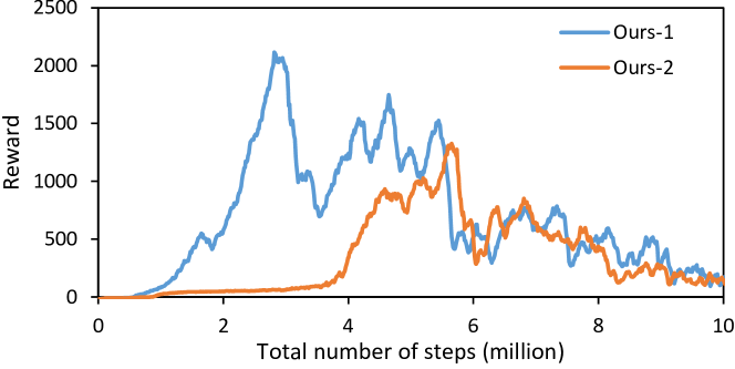
Figure 4: Transition of reward during training.

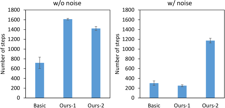
Figure 5: Result of simulation experiments for Basic, Ours-1, and Ours-2 controllers.

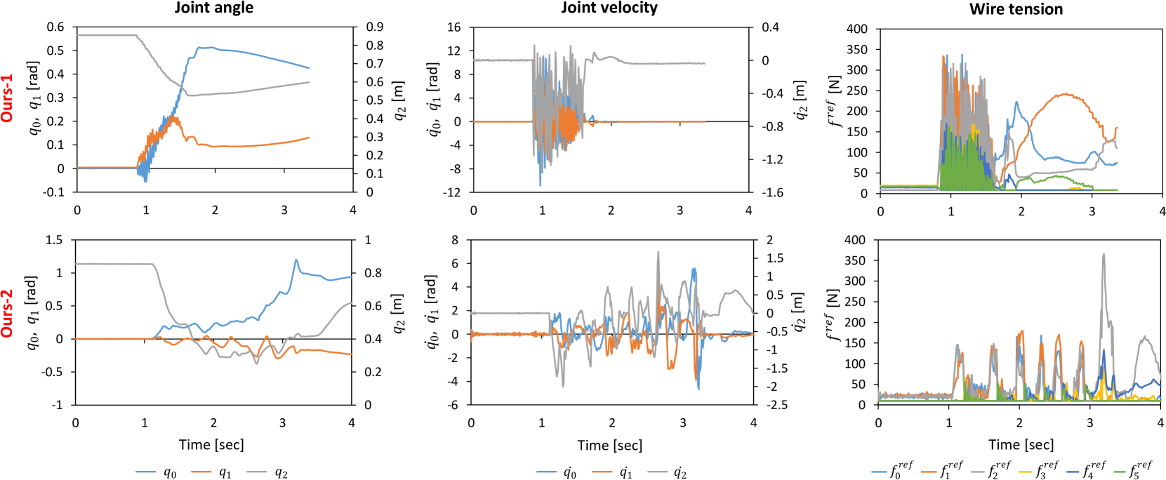
Figure 6: Result of the actual robot experiments for Ours-1 and Ours-2 controllers.

IV-B Actual Robot Experiment

The results of applying Ours-1 and Ours-2 to the actual robot are shown in Fig. 6. For the case of Ours-1, it can be seen that the wire length oscillates as wire tension is generated, and the estimated joint velocities accordingly oscillate and diverge significantly. As a result, the target wire tension output from the model also oscillates significantly, and the robot falls down without being able to jump even once.

On the other hand, for Ours-2, although the joint velocity oscillates slightly, the wire tension exerts appropriate force without being affected by the oscillation, and as a result, the robot is able to realize stable motion without divergence. In the present movement, the robot successfully jumped four times in succession. Because the body shifted in the translational direction, tension was applied to the apparatus suspending RAMIEL from above at the fifth jump.

V Discussion

We discuss the results of this study. First, a very dynamic and difficult task such as continuous jumping is made feasible with our reward, state, and action settings in reinforcement learning, with better performance than that of the method described in [8]. In this case, the joint velocity term is important, and it is shown that the learning progress is accelerated when this term is input as a state. On the other hand, since RAMIEL used in this study is driven by antagonistic wires, the effect of the oscillation of joint angles and joint velocities due to wire elongation cannot be ignored. In fact, when noise is applied to the wire length, the wire length, joint angle, and joint velocity oscillate accordingly. Therefore, while the performance of Ours-1 is better than that of Ours-2 without noise, that of Ours-1 is lower than that of Basic as well as Ours-2 in a noisy environment. Since joint angles are less prone to noise than joint velocities, the performance of Ours-2 does not deteriorate significantly in the noisy environment. This effect was more pronounced on the actual robot than in simulation. The oscillation of the wire length during the generation of wire tension on the actual robot was larger than expected, and Ours-1 could not jump even once. The oscillation of the joint velocity and that of the target wire tension alternated, causing the motion to diverge. On the other hand, Ours-2 was not significantly affected by the joint velocity oscillation, and the target wire tension was stable, resulting in smoother joint velocity transitions than Ours-1. Finally, the robot succeeded in making four consecutive jumps.

We discuss the problems and future prospects of this study. A significant progress has been made in this study in terms of the use of reinforcement learning and its applicability to the dynamic motion of a parallel wire-driven robot with wire elongation. On the other hand, we have not yet succeeded in achieving a complete continuous jumping motion. We believe that there are three reasons for this. (1) It is important to note that the friction of the body, especially the friction term in the joint motion and the loss of the output wire tension, does not match between the simulation and the actual robot. This corresponds to Actuator Net in [19], and Real2Sim using data from the actual robot is likely to be important. (2) We believe that it is necessary to add not only Gaussian noise but also steady-state error to the state. Depending on the installation of sensors, there are many cases where the noise is not only Gaussian noise but also biased noise. It is necessary to consider a noise design that takes such biases into account, as well as a method to reflect the steady-state error of the actual robot in the simulation. (3) The delay of observation and action needs to be dealt with. In particular, the body velocity output from Realsense T265, the joint angle estimation calculated from the wire length, and the delay from the motor control input to the wire tension generation due to the motor inertia need to be considered. We believe that when all of these problems are solved, stable continuous jumping motion will be realized on the actual robot.

VI CONCLUSION

In this study, we have developed a parallel wire-driven monopedal robot that can jump continuously using reinforcement learning. While parallel wire-driven robots have high jumping ability by gaining a long acceleration distance, they do not have a joint angle sensor in their minimum configuration, and the joint angle estimation from the wire length may oscillate significantly due to the elongation and loosening of the wire. To solve this problem, the time series of joint angles is used as the state input instead of the velocity term, which is susceptible to vibration. In addition, the definition of the reward function for a monopedal jumping robot and the method of noise generation for the application to the actual robot are presented. In the simulation, the results are much better than those of the previous control, and we can show some aspects of its application to the actual robot. We hope that this study will contribute to the realization of dynamic motions of parallel wire-driven robots.

References

- [1] D. W. Haldane, J. K. Yim, and R. S. Fearing, “Repetitive extreme-acceleration (14-g) spatial jumping with Salto-1P,” in Proceedings of the 2017 IEEE/RSJ International Conference on Intelligent Robots and Systems, 2017, pp. 3345–3351.
- [2] N. Kau, A. Schultz, N. Ferrante, and P. Slade, “Stanford doggo: An open-source, quasi-direct-drive quadruped,” in Proceedings of the 2019 IEEE International Conference on Robotics and Automation, 2019, pp. 6309–6315.
- [3] S. Kuindersma, R. Deits, M. Fallon, V. Andrës, H. Dai, F. Permenter, T. Koolen, P. Marion, and R. Tedrake, “Optimization-based locomotion planning, estimation, and control design for the atlas humanoid robot,” Autonomous Robots, vol. 40, pp. 429–455, 2016.
- [4] V. Zaitsev, O. Gvirsman, U. B. Hanan, A. Weiss, A. Ayali, and G. Kosa, “A locust-inspired miniature jumping robot,” Bioinspiration & Biomimetics, vol. 10, no. 6, 2015.
- [5] M. A. Woodward and M. Sitti, “MultiMo-Bat: A biologically inspired integrated jumpinggliding robot,” The International Journal of Robotics Research, vol. 33, no. 12, pp. 1511–1529, 2014.
- [6] T. Suzuki, Y. Toshimitsu, Y. Nagamatsu, K. Kawaharazuka, A. Miki, Y. Ribayashi, M. Bando, K. Kojima, Y. Kakiuchi, K. Okada, and M. Inaba, “RAMIEL: A Parallel-Wire Driven Monopedal Robot for High and Continuous Jumping,” in Proceedings of the 2022 IEEE/RSJ International Conference on Intelligent Robots and Systems, 2022, pp. 5017–5024.
- [7] S. Ookubo, Y. Asano, T. Kozuki, T. Shirai, K. Okada, and M. Inaba, “Learning Nonlinear Muscle-Joint State Mapping Toward Geometric Model-Free Tendon Driven Musculoskeletal Robots,” in Proceedings of the 2015 IEEE-RAS International Conference on Humanoid Robots, 2015, pp. 765–770.
- [8] M. H. Raibert, H. B. Brown, and M. Chepponis, “Experiments in Balance with a 3D One-Legged Hopping Machine,” The International Journal of Robotics Research, vol. 3, no. 2, pp. 75–92, 1984.
- [9] J. Schulman, F. Wolski, P. Dhariwal, A. Radford, and O. Klimov, “Proximal policy optimization algorithms,” arXiv preprint arXiv:1707.06347, 2017.
- [10] Y. Yang, K. Caluwaerts, A. Iscen, T. Zhang, J. Tan, and V. Sindhwani, “Data Efficient Reinforcement Learning for Legged Robots,” in Proceedings of the 2019 Conference on Robot Learning, 2019, pp. 1–10.
- [11] T. Miki, J. Lee, J. Hwangbo, L. Wellhausen, V. Koltun, and M. Hutter, “Learning robust perceptive locomotion for quadrupedal robots in the wild,” Science Robotics, vol. 7, no. 62, 2022.
- [12] A. Diamond and O. E. Holland, “Reaching control of a full-torso, modelled musculoskeletal robot using muscle synergies emergent under reinforcement learning,” Bioinspiration & Biomimetics, vol. 9, no. 1, pp. 1–16, 2014.
- [13] A. Marjaninejad, D. Urbina-Melëndez, B. A. Cohn, and F. J. Valero-Cuevas, “Autonomous functional movements in a tendon-driven limb via limited experience,” Nature Machine Intelligence, vol. 1, no. 3, pp. 144–154, 2019.
- [14] A. Grimshaw and J. Oyekan, “Applying Deep Reinforcement Learning to Cable Driven Parallel Robots for Balancing Unstable Loads: A Ball Case Study,” Frontiers in Robotics and AI, vol. 7, 2021.
- [15] F. Sugai, K. Kojima, Y. Kakiuchi, K. Okada, and M. Inaba, “Design of tiny high-power motor driver without liquid cooling for humanoid jaxon,” in Proceedings of the 2018 IEEE-RAS International Conference on Humanoid Robots, 2018, pp. 1059–1066.
- [16] E. Todorov, T. Erez, and Y. Tassa, “MuJoCo: A physics engine for model-based control,” in Proceedings of the 2012 IEEE/RSJ International Conference on Intelligent Robots and Systems, 2012, pp. 5026–5033.
- [17] A. Raffin, A. Hill, A. Gleave, A. Kanervisto, M. Ernestus, and N. Dormann, “Stable-Baselines3: Reliable Reinforcement Learning Implementations,” Journal of Machine Learning Research, vol. 22, no. 268, pp. 1–8, 2021.
- [18] S. Madgwick, “An efficient orientation filter for inertial and inertial/magnetic sensor arrays,” Report x-io and University of Bristol (UK), vol. 25, pp. 113–118, 2010.
- [19] J. Hwangbo, J. Lee, A. Dosovitskiy, D. Bellicoso, V. Tsounis, V. Koltun, and M. Hutter, “Learning agile and dynamic motor skills for legged robots,” Science Robotics, vol. 4, no. 26, 2019.