Learning-Based Wiping Behavior of Low-Rigidity Robots Considering Various Surface Materials and Task Definitions

Abstract

Wiping behavior is a task of tracing the surface of an object while feeling the force with the palm of the hand. It is necessary to adjust the force and posture appropriately considering the various contact conditions felt by the hand. Several studies have been conducted on the wiping motion, however, these studies have only dealt with a single surface material, and have only considered the application of the amount of appropriate force, lacking intelligent movements to ensure that the force is applied either evenly to the entire surface or to a certain area. Depending on the surface material, the hand posture and pressing force should be varied appropriately, and this is highly dependent on the definition of the task. Also, most of the movements are executed by high-rigidity robots that are easy to model, and few movements are executed by robots that are low-rigidity but therefore have a small risk of damage due to excessive contact. So, in this study, we develop a method of motion generation based on the learned prediction of contact force during the wiping motion of a low-rigidity robot. We show that MyCobot, which is made of low-rigidity resin, can appropriately perform wiping behaviors on a plane with multiple surface materials based on various task definitions.

I INTRODUCTION

Wiping behavior is a basic human motion of tracing the surface of an object while feeling the force with the palm of the hand. It is necessary to adjust the force, hand posture, etc. appropriately considering the various contact conditions felt by the hand. Several studies have been conducted on this wiping motion [1]. [2] has formulated and discussed the generation of trajectories for wiping 3D surfaces as a traveling salesman problem. [3] has developed a method for generating trajectories that wipe 3D surfaces using dynamic motion primitives and avoiding restricted areas. [4] has generated wiping motions on 2D surfaces using imitation learning based on visual, tactile, and joint information, and extended this method to 3D surfaces including occlusion [5]. [6] has generated wiping motions on a 2D plane by reinforcement learning with variable impedance control as a control input. [7] furthermore automatically adjusts the gain of the variable impedance control to enable wiping operation on several surface materials. As shown above, it is now possible to generate trajectories using a general geometric model, position control, torque control, imitation learning, and reinforcement learning.

On the other hand, we believe that these studies have three problems. (1) They usually deal with only a single type of surface material and lack flexibility. In reality, the surfaces to be wiped vary from smooth floors to rough desks and uneven walls. (2) They only apply a constant force in an appropriate direction, and lack intelligent motion generation such as checking whether the force is applied either evenly to the entire contact surface, or daring to a certain area. (3) Most of the experiments have been conducted with high-rigidity robots that are easy to model and can execute movements accurately, but not with robots that are less rigid and therefore have less risk of damage due to excessive contact. If this becomes possible, the task can be performed with less expensive and less capable robots. The objective of this study is to solve these problems (1)–(3) to realize a more adaptive wiping motion.

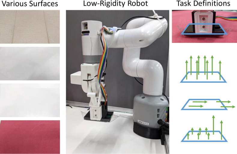
Figure 1: The concept of this study: we handle wiping behaviors with (1) various surface materials, (2) various task definitions, and (3) low-rigidity robot.

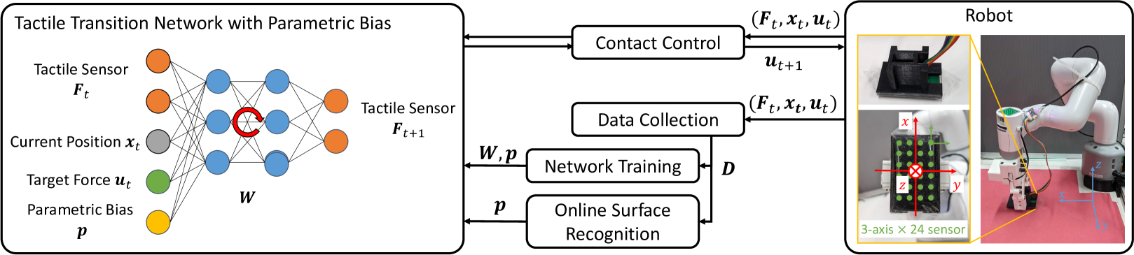
Figure 2: The overview of the learning system of this study.

To solve (3), we conduct experiments using an actual robot, MyCobot, which is made of low-rigidity resin and has difficulty in performing accurate movements. We collect data from the motion of the robot by adding random noise to a simple proportional control, and construct a contact transition model by learning a neural network, which takes into account the softness and rattling of the robot. To solve (1), we use a learnable input variable, parametric bias [8, 9], which can extract multiple attractor dynamics from various data, to deal with different surface materials. Parametric bias has been mainly used for imitation learning, but we are now applying it to predictive model learning [10, 11, 12]. To solve (2), we use a contact sensor, uSkin [13], which contains 24 3-axis sensors in an area of 31 mm $\times$ 51.5 mm. We show that various task definitions can be created for the contact and friction forces by setting appropriate loss functions for these 72 dimensional values. In order to focus on solving (1)–(3), we limit our experiments to a two-dimensional plane instead of a three-dimensional surface.

This study is organized as follows. In Section I, the background and purpose of this study are described. In Section II, we describe a network configuration for representing the state transitions of contact sensors, data collection with random noise added to proportional control, network training, recognition of surface material properties, and contact control for various task definitions. In Section III, we conduct experiments using an actual low-rigidity robot, MyCobot. Finally, in Section IV, we discuss the results, and in Section V, we conclude and give some future perspectives.

II Learning-Based Wiping Behavior of Low-Rigidity Robots Considering Various Surfaces and Task Definitions

The overall system of this study is shown in Fig. 2. In this study, a low-rigidity robot MyCobot is used. As shown in the right figure of Fig. 2, MyCobot is equipped with a contact sensor, uSkin, which contains 24 3-axis force sensors on its tip end, which is pressed against the surface to be wiped. Data is collected by Data Collector and the proposed Tactile Transition Network with Parametric Bias (TTNPB) is trained. By updating PB online from the current data, the robot can recognize the surface material and perform the wiping operation by controlling the contact according to the desired task definition.

II-A Network Structure

The network structure of TTNPB constructed in this study can be expressed as follows:

$$\bm{F}_{t+1}=\bm{h}_{ttnpb}(\bm{F}_{t},\bm{x}_{t},\bm{u}_{t},\bm{p})$$ (1)

where $t$ is the current time step, $\bm{F}$ is the contact sensor value, $\bm{x}$ is the current hand position, $\bm{u}$ is the control input, $\bm{p}$ is parametric bias (PB), and $\bm{h}_{ttnpb}$ is the prediction model. This model represents the transition of contact sensor values when a control input is applied at the current position. Since the rattling of a low-rigidity robot body varies depending on its posture, $\bm{x}_{t}$ is added as a network input. The contact sensor value $\bm{F}$ provides $xyz$ 3-axis force data for a total of 24 (4$\times$6) locations as shown in the right figure of Fig. 2. No force calibration is performed except for the removal of offsets, and the data is handled as dimensionless values. $\bm{F}_{\{x,y,z\}}$ denotes the 24-dimensional vector of forces in each direction, and $F^{ave}_{\{x,y,z\}}$ denotes the average of forces in each direction.

The control input $\bm{u}$ consists of $\{\tau^{ref}_{roll},\tau^{ref}_{pitch},f^{ref}_{z}\}$, and the following proportional control changes the actual robot hand position and orientation:

$$\Delta\theta^{ref}_{roll} =\max(\Delta\theta^{min},\min(k_{\theta}(\tau^{ref}_{roll}-\tau_{roll}),\Delta\theta^{max}))$$ (2)

$$\Delta\theta^{ref}_{pitch} =\max(\Delta\theta^{min},\min(k_{\theta}(\tau^{ref}_{pitch}-\tau_{pitch}),\Delta\theta^{max}))$$ (3)

$$\Delta{x}^{ref}_{z} =\max(\Delta{x}^{min}_{z},\min(k_{z}(f^{ref}_{z}-F^{ave}_{z}),\Delta{x}^{max}_{z}))$$ (4)

$$\theta^{ref}_{roll} \leftarrow\max(\theta^{min},\min(\theta^{ref}_{roll}+\Delta\theta^{ref}_{roll},\theta^{max}))$$ (5)

$$\theta^{ref}_{pitch} \leftarrow\max(\theta^{min},\min(\theta^{ref}_{pitch}+\Delta\theta^{ref}_{pitch},\theta^{max}))$$ (6)

$$x^{ref}_{z} \leftarrow x^{ref}_{z}+\Delta{x}^{ref}_{z}$$ (7)

where $\theta^{ref}_{\{roll,pitch,yaw\}}$ is the target hand angle, $x^{ref}_{\{x,y,z\}}$ is the target hand position, $\tau^{ref}_{\{roll,pitch\}}$ is the target torque around the center axis of the contact sensor regarding the roll and pitch axis, $\tau_{\{roll,pitch\}}$ is the current torque around the center axis of the contact sensor, $f^{ref}_{z}$ is the target value of $F^{ave}_{z}$, $k_{\{\theta,z\}}$ is the constant gain of proportional control, and $\{\Delta\theta,\theta,\Delta{x}_{z}\}^{\{min,max\}}$ are the minimum and maximum values of $\{\Delta\theta,\theta,\Delta{x}_{z}\}$. The minimum and maximum settings for $x_{z}$ are excluded because of the possibility of large changes in the $x_{z}$ direction. For $\tau_{\{roll,pitch\}}$, since the distances between the 24 3-axis force sensors are known, it is possible to calculate the current torque using the moment around the center axis of the contact sensors. In addition, by setting the target hand angle $\theta^{ref}_{yaw}$ around the yaw axis to 0 and the hand position $x^{ref}_{\{x,y\}}$ in $xy$ direction to arbitrary values, the hand posture $\bm{\theta}^{ref}$ and $\bm{x}^{ref}$ are obtained. By solving inverse kinematics on this posture, the target joint angles $\bm{q}^{ref}$ of the robot are obtained and sent to the actual robot. Note that even if $\bm{q}^{ref}$ is sent to the robot, it is not possible to realize the exact $\bm{q}^{ref}$ because of the low rigidity of the robot, and a learning mechanism is required.

Parametric bias $\bm{p}$ is a learnable input variable in neural networks. When data with multiple dynamics are collected and trained in a single network, the parameters related to the dynamics that do not fit into the single model self-organize in the space of parametric bias. By changing this parameter, the dynamics of $\bm{h}_{ttnpb}$ can be changed to adapt to various surface materials.

The details of the network configuration are described below. In this study, TTNPB consists of 10 layers, which is made up of 4 FC layers (fully-connected layers), 2 LSTM layers (long short-term memory layers) [14], and 4 FC layers, in order. For the number of hidden units, we set {$N_{F}+N_{x}+N_{u}+N_{p}$, 300, 200, 100, 100 (number of units in LSTM), 100 (number of units in LSTM), 100, 200, 300, $N_{F}$} (note that $N_{\{F,x,u,p\}}$ is the number of dimensions of $\{\bm{F},\bm{x},\bm{u},\bm{p}\}$). The activation function is hyperbolic tangent and the update rule is Adam [15]. $\bm{p}$ is two-dimensional, and the execution period of Eq. 1 is set to 5 Hz. The dimensionality of $\bm{p}$ should be slightly smaller than the expected changes in the body state, because too small a dimensionality will not represent changes in dynamics properly, and too large a dimensionality will make self-organization difficult. Also, we set $k_{\{\theta,z\}}=\{0.01,0.03\}$, $\Delta\theta^{\{min,max\}}=\{-3.0,3.0\}$ [deg], $\theta^{\{min,max\}}=\{-5.0,5.0\}$ [deg], and $\Delta{x}_{z}^{\{min,max\}}=\{-5.0,5.0\}$ [mm].

II-B Data Collection

We describe the data collection method. For $\bm{x}$ in the $xy$ direction, the motion is arbitrarily specified, and $\bm{u}$ is changed as follows.

$$\tau^{ref}_{roll} \leftarrow\max(\tau^{min},\min(\tau^{ref}_{roll}+N(0,\sigma_{\theta}),\tau^{max}))$$ (8)

$$\tau^{ref}_{pitch} \leftarrow\max(\tau^{min},\min(\tau^{ref}_{pitch}+N(0,\sigma_{\theta}),\tau^{max}))$$ (9)

$$f^{ref}_{z} \leftarrow\max(f^{min},\min(f^{ref}_{z}+N(0,\sigma_{z}),f^{max}))$$ (10)

where $N(\mu,\sigma)$ is the Gaussian noise with mean $\mu$ and variance $\sigma$, $\sigma_{\{\theta,z\}}$ is the variance of the data collection for each direction, $\tau^{\{min,max\}}$ are the minimum and maximum values of $\tau$, and $f^{\{min,max\}}$ denotes the minimum and maximum values of $f$. By gradually changing $\bm{u}$ within the minimum and maximum values, the target values of the proportional control can be shifted and various data can be obtained. In this study, we set $\sigma_{\{\theta,z\}}=\{10,30\}\;\textrm{or}\;\{3,10\}$, $\tau^{\{min,max\}}=\{-50,50\}$, and $f^{\{min,max\}}=\{50,300\}$. As described above, we collect data by changing $\sigma_{\{\theta,z\}}$ to two different values. Note that since $F$ is dimensionless, $f$ and $\tau$ are also handled to be dimensionless.

II-C Training of TTNPB

The obtained data $D$ is used to train TTNPB. By collecting data while changing the surface material, the data can be implicitly embedded in the parametric bias. In order to represent each time series transition with different dynamics in a single model, we embed the differences in the dynamics into a low-dimensional space of $\bm{p}$. In this case, no labeling of data is required. The data collected on the same surface material $k$ is represented as $D_{k}=\{(\bm{F}_{1},\bm{x}_{1},\bm{u}_{1}),(\bm{F}_{2},\bm{x}_{2},\bm{u}_{2}),\cdots,(\bm{F}_{T_{k}},\bm{x}_{T_{k}},\bm{u}_{T_{k}})\}$ ($1\leq k\leq K$, where $K$ is the total number of trials and $T_{k}$ is the number of steps of the trial for surface material $k$), and the data for learning, $D_{train}=\{(D_{1},\bm{p}_{1}),(D_{2},\bm{p}_{2}),\cdots,(D_{K},\bm{p}_{K})\}$, is obtained. Here, $\bm{p}_{K}$ is the parametric bias expressing the dynamics in the surface material $k$, which is a common variable for that surface and another variable for another surface. TTNPB is trained using this $D_{train}$. In the usual training, only the network weight $W$ is updated, but here $W$ and $p_{k}$ for each state are updated at the same time. This means that $p_{k}$ is embedded with the difference in the dynamics of each surface material. Mean-squared error is used as the loss function during training, and $\bm{p}_{k}$ is optimized with all initial values set to 0.

II-D Online Recognition of Surface Being Wiped

Parametric bias $\bm{p}_{k}$ obtained in the previous section is the value at training time, and the current $\bm{p}$ should be appropriate for the current surface material. Using the data $D$ obtained for the current state, the current surface material can be estimated by updating the parametric bias online. Since only low-dimensional parametric bias $\bm{p}$ is updated, overfitting is unlikely to occur and the system can keep learning. This online learning process allows us to obtain a model that is always adapted to the current surface material.

The number of data obtained is set as $N^{online}_{data}$, and online learning starts when the number of data exceeds $N^{online}_{thre}$. Each time new data is received, training is performed with $N^{online}_{batch}$ for the number of batches, $N^{online}_{epoch}$ for the number of epochs, and MomentumSGD for the update rule. Data exceeding $N^{online}_{max}$ are deleted from the oldest ones.

In this study, we set $N^{online}_{\{thre,max\}}=\{10,30\}$, $N^{online}_{batch}=N^{online}_{max}$, and $N^{online}_{epoch}=3$.

II-E Contact Control with Various Task Definitions

We describe the generation of wiping motion using TTNPB. We optimize $\bm{u}$ from the loss functions on $\bm{F}$ and $\bm{u}$. First, we give the initial value $\bm{u}^{init}_{seq}$ of the time series control input $\bm{u}_{seq}=\bm{u}_{[t:t+N_{step}-1]}$ ($N_{step}$ is the number of TTNPB expansions in the control, or control horizon). Let $\bm{u}$ to be optimized be $\bm{u}^{opt}_{seq}$, and repeat the following calculation at time $t$ to obtain the optimal $\bm{u}^{opt}_{t}$.

$$\bm{F}^{pred}_{seq} =\bm{h}_{expand}(\bm{F}_{t},\bm{x}_{t},\bm{u}^{opt}_{seq})$$ (12)

$$L =\bm{h}_{loss}(\bm{F}^{pred}_{seq},\bm{u}^{opt}_{seq})$$ (13)

$$\bm{u}^{opt}_{seq} \leftarrow\bm{u}^{opt}_{seq}-\gamma\partial{L}/\partial{\bm{u}^{opt}_{seq}}$$ (14)

where $\bm{F}^{pred}_{seq}$ is the predicted $\bm{F}_{[t+1:t+N_{step}]}$, $\bm{h}_{expand}$ is the function $\bm{h}$ expanded $N_{step}$ times, $\bm{h}_{loss}$ is the loss function, and $\gamma$ denotes the learning rate. In other words, the future $\bm{F}$ is predicted from the current state $\bm{F}_{t}$ and $\bm{x}_{t}$ by the time series control input $\bm{u}^{opt}_{seq}$, and $\bm{u}^{opt}_{seq}$ is calculated to minimize the loss function set for it using the backpropagation technique and gradient descent method.

Here, we set $\bm{u}^{init}_{seq}$ as $\bm{u}^{prev}_{\{t+1,\cdots,t+N_{step}-1,t+N_{step}-1\}}$ by using $\bm{u}^{prev}_{[t:t+N_{step}-1]}$ (which is $\bm{u}_{seq}$ optimized in the previous step) shifting it one time step, and duplicating the last term. Faster convergence can be obtained by using the previous optimization results. For $\gamma$, $[0,\gamma_{max}]$ is exponentially divided into $N^{control}_{batch}$ $\gamma$, and after running Eq. 14 on each $\gamma$, $\bm{u}^{opt}_{seq}$ with the smallest loss is selected by computing the loss with Eq. 13, repeating the process $N^{control}_{epoch}$ times. Faster convergence can be obtained by always choosing the best learning rate while trying various $\gamma$.

Here, the loss function $\bm{h}_{loss}$ allows for various task definitions. In this study, we set $\bm{h}_{loss}$ to the following three types and conduct experiments with them.

$$h_{loss,1}(\bm{F}^{pred}_{seq}) =||\bm{F}^{pred}_{z,seq}-\bm{F}^{ref}_{z,seq}||^{2}_{2}$$ (15)

$$h_{loss,2}(\bm{F}^{pred}_{seq}) =\textrm{Variance}(\bm{F}^{pred}_{y,seq})$$ (16)

$$h_{loss,3}(\bm{F}^{pred}_{seq}) =||\bm{F}^{pred}_{right-z,seq}-\bm{F}^{ref}_{seq}||^{2}_{2}+||\bm{F}^{pred}_{left-z,seq}||^{2}_{2}$$ (17)

where $\bm{F}^{ref}_{z}$ is the target value of $\bm{F}_{z}$, $||\cdot||_{2}$ is L2 norm, $\textrm{Variance}(\cdot)$ is the time direction average of the variance among sensors at that time, and $\bm{F}^{pred}_{\{right-z,left-z\}}$ is the $\bm{F}^{prev}_{z}$ values of the six rightmost sensors (right) and the rest (left) when the $x$-axis is set as the front. In other words, Eq. 15 is the error from the target value regarding $\bm{F}_{z}$, Eq. 16 is the variance regarding $\bm{F}_{y}$, and Eq. 17 is the loss that directs the force to the right regarding $\bm{F}_{z}$. In addition, we actually add loss that smoothes the transition of $\bm{u}^{pred}_{seq}$ to each loss.

In this study, we set $N_{step}=4$, $N^{control}_{batch}=5$, $N^{control}_{epoch}=3$, $\gamma_{max}=0.1$, and $F^{ref}_{z}=200$.

III Experiments

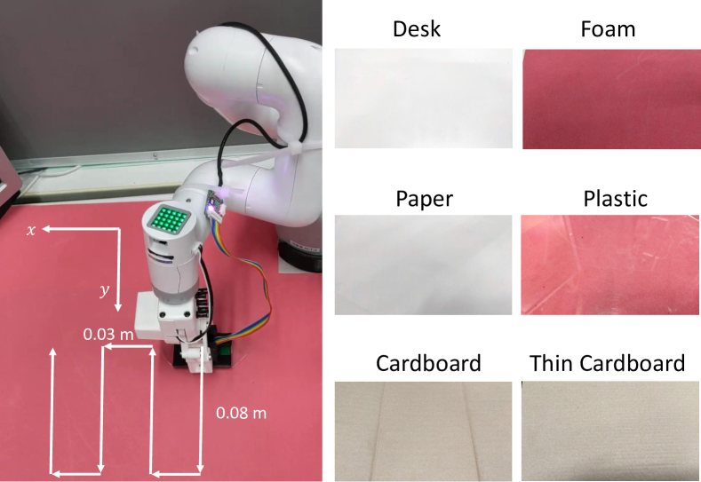
Figure 3: The experimental setup: the trajectory of wiping and various surface materials handled in this study.

III-A Experimental Setup

In this study, we conduct experiments on the six surface materials shown in the right figure of Fig. 3. Foam is a thin polyethylene foam sheet (2 mm), and Plastic is a thin plastic sheet (0.5 mm). Cardboard is thick (5 mm) and wavy, while Thin Cardboard is thin (2 mm) and neither as thick nor as wavy as Cardboard. For Paper, Plastic, and Thin Cardboard, the experiments were conducted with these sheets laid on top of Foam. The experiments are performed with a slippery tape material wrapped around the uSkin. The uSkin moves back and forth along the trajectory in the $xy$ direction as shown in the left figure of Fig. 3.

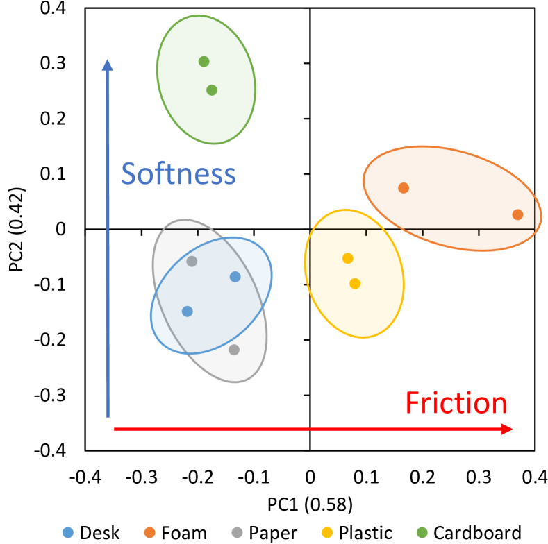
Figure 4: The arrangement of the trained parametric bias.

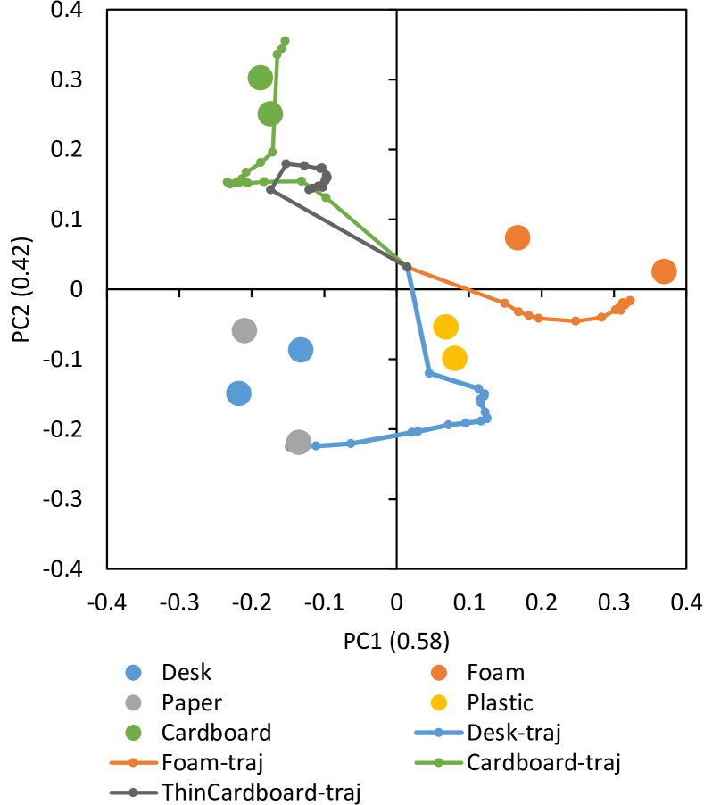
Figure 5: The trajectory of parametric bias while updating it online.

III-B Training of TTNPB and Online Learning of Parametric Bias

First, we collect data for the five surface materials in Fig. 3, excluding Thin Cardboard, by the method of Section II-B. In this case, we change $\sigma_{\{\theta,z\}}$ to two different values as described in Section II-B. By acquiring data for about 1000 steps in each setting, we use a total of about 10000 data points for training. Fig. 4 shows the arrangement of PBs obtained from the training in a 2-dimensional plane by applying Principle Component Analysis (PCA). In this study, $\bm{p}$ is set to two dimensions, but even in this case, the principal axes can be obtained by PCA. Even when $\sigma$ is set differently, when the surface materials are the same, PBs are placed close to each other because the tactile dynamics are the same. It is also considered that PC1 qualitatively represents the axis related to the friction of the surface, and PC2 represents the softness of the surface material. Cardboard, Desk, and Paper are very similar in terms of their surface friction, and the friction between each of them and the material of the contact sensor is smaller than that of Plastic and Foam. In terms of the softness of the surface materials, Desk, Paper, and Plastic are rigid, and Foam and Cardboard are soft, in that order. In other words, even if we do not directly provide the label of the material, it is possible to self-organize the space of PB autonomously depending on whether the dynamics of the material is close or far from another surface material.

Next, we conducted experiments on the recognition of surface materials. We performed the same random motion as in the training phase, with the four surface materials (Desk, Foam, Cardboard, and Thin Cardboard). The trajectory of PB when executing Section II-D is shown in Fig. 5 as “-traj”. It can be seen that the current PBs of Cardboard, Desk, and Foam are each moving toward PBs obtained at the time of training. Thin Cardboard is a surface material that was not used in the training, but its trajectory is located slightly below the $\bm{p}_{k}$ of Cardboard. This result is consistent with the fact that Thin Cardboard is thinner than Cardboard and thus its surface softness is reduced, while the surface friction does not change much because the material itself is the same. For both the surface material used in the training and the unknown surface material, the current dynamics were explored appropriately in the space of PB.

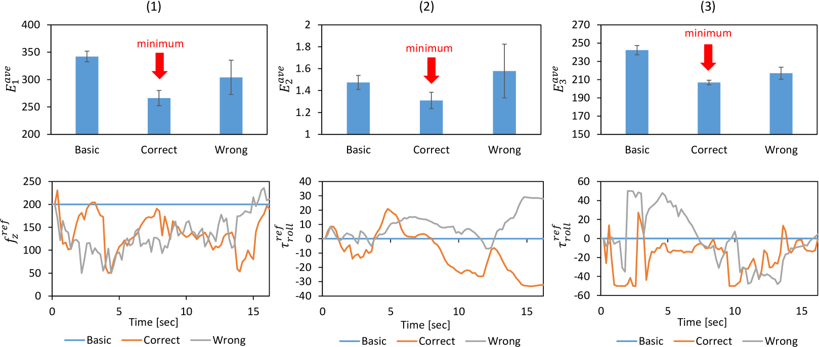
Figure 6: The evaluation value $E^{ave}$ and the transition of the most important control inputs for wiping control with Basic, Correct, and Wrong controllers with loss (1) – (3).

III-C Wiping Behavior Considering Various Surfaces and Task Definitions

The three loss functions defined in Section II-E are used to execute the wiping operation in each task definition. Let Foam be the surface material, Correct be the case where Section II-E is executed with the trained PB of Foam, and Wrong be the case where Section II-E is executed using PB of a different material, Desk. The case where the variance is set to 0 in Section II-B is called Basic and is used for comparison. The results of the control of Basic, Correct, and Wrong for the three loss functions (the experiments with each loss function are called (1), (2), and (3), respectively) are shown in Fig. 6. Here, the control by each loss function is evaluated by the average $E^{ave}$ of the evaluation values $E$ of the same number as shown below:

$$E_{1} =||\bm{F}_{z}-\bm{F}^{ref}_{z}||_{2}$$ (18)

$$E_{2} =\textrm{Std}(\bm{F}_{y})/F^{abs-ave}_{y}$$ (19)

$$E_{3} =||\bm{F}_{right-z}-\bm{F}^{ref}||_{2}+||\bm{F}_{left-z}||_{2}$$ (20)

where $\textrm{Std}(\cdot)$ denotes the standard deviation, and $F^{abs-ave}_{y}$ denotes the mean of the absolute values of $\bm{F}_{y}$. For $E_{2}$, since the standard deviation increases as the absolute value of $F_{y}$ increases, the value is evaluated by dividing it by $F^{abs-ave}_{y}$. The smaller this evaluation value is, the better. We also show the transition of $F^{ref}$ for (1) and $\tau_{roll}$ for (2) and (3) as the most important values of $\bm{u}$ in the control for each loss function.

For each loss, the Correct case generates the best controller with the smallest $E^{ave}$. For (1), the generated $F^{ref}_{z}$ transitions show that both Correct and Wrong output smaller values than $F^{ref}_{z}$, which is constant in Basic. This may be due to the fact that in Basic, where $F^{ref}_{z}=200$ is constant, the tips of the hand are often caught by the surface materials and a large $\bm{F}_{z}$ is generated, causing a large increase in Eq. 15. Therefore, a value smaller than $F^{ref}_{z}=200$ is properly output in alignment with the current $\bm{x}$. As for (2), the transition of the generated $\tau^{ref}_{roll}$ shows that $\tau^{ref}_{roll}$ repeatedly increases and decreases along with the motion. Since the direction of motion changes about the $y$-axis as in Fig. 3 in this study, the roll angle is changed accordingly to avoid a situation where the sensor is trapped by the surface material or a strong force is applied to some of the sensors. As for (3), the generated transition of $\tau^{ref}_{roll}$ shows that it swings in the negative direction, especially for Correct. Since the purpose of this experiment is to move the contact sensor by applying force to the right side of the sensor and not to the left side, the torque in the roll direction that is applied to the contact sensor becomes as negative as possible.

IV Discussion

We discuss the experimental results in this study. First, parametric bias was able to self-organize the dynamics of surface materials into the space of PB based on the differences in dynamics among the data, even without providing explicit labels. The dynamics are automatically classified by human intuitive axes such as surface friction and surface softness. By updating only the parametric bias, it was possible to recognize the surface material currently being wiped from the current data. It was also shown that the model can be applied to unknown surface materials. Next, it was found that the model can be used to represent various tasks by loss functions. The loss function can be freely taken for the contact sensor values, and the task representation can be changed. Our method outperforms the default controller with constant control input. On the other hand, the performance may suffer if the current recognition of the surface material is not accurate, and so it is necessary to simultaneously recognize the surface material and control the contact.

The limitations of this study are as follows. In this study, the experiment was conducted by first establishing proportional control, and then changing the target value of the proportional control, which resulted in stable operation. Although it is possible to use angular velocity and other parameters directly as control inputs without proportional control, it caused the behavior to become very unstable. The use of more complicated control inputs is a future task to solve. In addition, this study deals only with two-dimensional planes. Of course, there is a possibility that 3D surfaces can also be handled, but since feedback alone is not sufficient for this, it is necessary to combine this method with trajectory generation based on shape recognition using images and point clouds. This is also a challenge for the future.

V CONCLUSION

In this study, we have constructed a neural network representing state transitions of contact sensors in order to realize a wiping motion applicable to various surface materials and task definitions. The network is trained by collecting data from the motion with random noise added to the proportional control. By using parametric bias as a network input, information on the characteristics of the surface material can be embedded in the network. The current properties of the surface material can be estimated from the contact state transitions, and the motion can be changed accordingly. By changing the loss function related to the contact state according to the task, it is possible to apply force evenly or to only certain areas. In addition, we have shown through experiments that these learning behaviors can be applied to a low-rigidity robot that has difficulty in making precise movements. As this study dealt only with two-dimensional planes, we would like to apply this method to three-dimensional curved surfaces to make it possible to execute motions in a more practical manner.

References

- [1] J. Kim, A. K. Mishra, R. Limosani, M. Scafuro, N. Cauli, J. Santos-Victor, B. Mazzolai, and F. Cavallo, “Control strategies for cleaning robots in domestic applications: A comprehensive review,” International Journal of Advanced Robotic Systems, vol. 16, no. 4, pp. 1–21, 2019.
- [2] J. Hess, G. D. Tipaldi, and W. Burgard, “Null space optimization for effective coverage of 3D surfaces using redundant manipulators,” in Proceedings of the 2012 IEEE/RSJ International Conference on Intelligent Robots and Systems, 2012, pp. 1923–1928.
- [3] A. C. Dometios, Y. Zhou, X. S. Papageorgiou, C. S. Tzafestas, and T. Asfour, “Vision-Based Online Adaptation of Motion Primitives to Dynamic Surfaces: Application to an Interactive Robotic Wiping Task,” IEEE Robotics and Automation Letters, vol. 3, no. 3, pp. 1410–1417, 2018.
- [4] N. Saito, D. Wang, T. Ogata, H. Mori, and S. Sugano, “Wiping 3D-objects using Deep Learning Model based on Image/Force/Joint Information,” in Proceedings of the 2020 IEEE/RSJ International Conference on Intelligent Robots and Systems, 2020, pp. 10 152–10 157.
- [5] N. Saito, T. Shimizu, T. Ogata, and S. Sugano, “Utilization of Image/Force/Tactile Sensor Data for Object-Shape-Oriented Manipulation: Wiping Objects With Turning Back Motions and Occlusion,” IEEE Robotics and Automation Letters, vol. 7, no. 2, pp. 968–975, 2022.
- [6] R. Martín-Martín, M. A. Lee, R. Gardner, S. Savarese, J. Bohg, and A. Garg, “Variable Impedance Control in End-Effector Space: An Action Space for Reinforcement Learning in Contact-Rich Tasks,” in Proceedings of the 2019 IEEE/RSJ International Conference on Intelligent Robots and Systems, 2019, pp. 1010–1017.
- [7] C. Wang, Z. Kuang, X. Zhang, and M. Tomizuka, “Safe Online Gain Optimization for Variable Impedance Control,” arXiv preprint arXiv:2111.01258, 2019.
- [8] J. Tani, “Self-organization of behavioral primitives as multiple attractor dynamics: a robot experiment,” in Proceedings of the 2002 International Joint Conference on Neural Networks, 2002, pp. 489–494.
- [9] J. Tani, M. Ito, and Y. Sugita, “Self-organization of distributedly represented multiple behavior schemata in a mirror system: reviews of robot experiments using RNNPB,” Neural Networks, vol. 17, no. 8, pp. 1273–1289, 2004.
- [10] K. Kawaharazuka, K. Tsuzuki, M. Onitsuka, Y. Asano, K. Okada, K. Kawasaki, and M. Inaba, “Object Recognition, Dynamic Contact Simulation, Detection, and Control of the Flexible Musculoskeletal Hand Using a Recurrent Neural Network With Parametric Bias,” IEEE Robotics and Automation Letters, vol. 5, no. 3, pp. 4580–4587, 2020.
- [11] K. Kawaharazuka, A. Miki, M. Bando, K. Okada, and M. Inaba, “Dynamic Cloth Manipulation Considering Variable Stiffness and Material Change Using Deep Predictive Model With Parametric Bias,” Frontiers in Neurorobotics, vol. 16, pp. 1–16, 2022.
- [12] K. Kawaharazuka, N. Kanazawa, K. Okada, and M. Inaba, “Self-Supervised Learning of Visual Servoing for Low-Rigidity Robots Considering Temporal Body Changes,” IEEE Robotics and Automation Letters, vol. 7, no. 3, pp. 7881–7887, 2022.
- [13] T. P. Tomo, A. Schmitz, W. K. Wong, H. Kristanto, S. Somlor, J. Hwang, L. Jamone, and S. Sugano, “Covering a Robot Fingertip With uSkin: A Soft Electronic Skin With Distributed 3-Axis Force Sensitive Elements for Robot Hands,” IEEE Robotics and Automation Letters, vol. 3, no. 1, pp. 124–131, 2018.
- [14] S. Hochreiter and J. Schmidhuber, “Long short-term memory,” Neural computation, vol. 9, no. 8, pp. 1735–1780, 1997.
- [15] D. P. Kingma and J. Ba, “Adam: A Method for Stochastic Optimization,” in Proceedings of the 3rd International Conference on Learning Representations, 2015, pp. 1–15.