Merons and magnetoelectric switching in centrosymmetric spiral magnets

Abstract

Spiral multiferroics exhibit a strong coupling between magnetic and ferroelectric orders, allowing cross-control. Since the seminal work of Kimura et al. in 2003, these materials have attracted great interest galvanized by the prospect of new high-efficiency memory devices, where magnetic (electric) bits are switched via an external electric (magnetic) field. Nevertheless, the mechanism underlying such a switching process—the electric field-driven dynamics of domain walls (DWs)—is still poorly understood. We address this problem for meron DWs, which represent one of the main DW types in spiral multiferroics and consist of an array of meron (half-skyrmion) strings. Minimum energy walls feature merons with alternating topological charges and move as relativistic massive particles, with the limiting velocity set by magnon speed. Low-energy defects in this alternating charge sequence, which appear during domain nucleation, can lead to DWs with net topological charge. This induces a peculiar non-local dynamics where all the spins in the system rotate, merons translate within the wall, and the DW mobility is suppressed. The topological charge of the wall and the meron helicity can be easily modified via an external magnetic and electric field, respectively, offering fine control over DW dynamics. Defects within the meron strings, analogous to Bloch points, have hedgehog-like spin texture and are strongly pinned to the lattice. The fascinating interplay between domain wall motion, translation of merons within the wall, and precession of spins in the entire domains opens a new playground for the electric manipulation of topological spin textures.

Introduction. —

Domain wall (DW) motion in magnetic materials is a subject of both fundamental and technological interest [1, 2, 3, 4, 5, 6]. Indeed, switching between two states of a magnetic bit proceeds through the nucleation, propagation and annihilation of DWs. The existing magnetic storage devices use a magnetic field to record (i.e., drive the DWs), leading to considerable power consumption and limiting information density. Multiferroic materials combine multiple coexisting orders and enable cross-control, particularly the electric control of magnetization [7, 8, 9, 10, 11]. This functionality allows to drive magnetic DWs by an electric field for a drastically more efficient switching process [12].

The most basic non-collinear magnets, spiral magnets, are also prototypical magnetoelectric multiferroics. The magnetic spiral breaks inversion symmetry and induces a ferroelectric polarization ${\bf P}\propto[\hat{n}\times{\bf Q}]$, where $\hat{n}$ is the unit normal to the spin rotation plane and $\bf{Q}$ is the spiral wave vector [9]. $\bf{P}$ is non-zero for a cycloidal spiral, for which the spin rotation plane contains $\bf{Q}$. The DW between two spiral domains with opposite chirality consists of an array of vortex or meron (half-skyrmion [13, 14, 15]) strings (see Fig. 1), except for a few wall orientations [16]. The existing literature focuses on (vortex-free) Hubert DWs [17, 18, 5] and on vortex DWs [16, 18, 19, 20]. Meron DWs, which arise when the anisotropy is weaker, are still widely unexplored. Nevertheless, most of the experimental realizations of spiral magnets (e.g. CuO, MnWO₄, Ni₃V₂O₈, LiCu₂O₂, and LiCuVO₄ [21]) are in this weak anisotropy regime. In particular, electric field-induced switching has been experimentally studied in MnWO₄ [22, 23]. The results suggest that the spiral plane rotates across the wall, consistent with meron DWs (see Fig. 1) but not with vortex DWs. Moreover, Hubert DWs have only one possible orientation (i.e. perpendicular to the wave vector). Since two preferred wall orientations are observed, at least one corresponds to meron DWs.

We analyze the structure and the electric field-driven dynamics of meron DWs in cycloidal spiral magnets by combining the Ginzburg-Landau approach, the collective coordinates method [3, 4], and atomistic spin dynamics simulations [24]. The dynamics of the minimum energy DW, for which the meron topological charges alternate, reduces to that of a “relativistic” massive particle, where the maximum magnon velocity plays the role of the speed of light. Low-energy defects, corresponding to neighboring merons with the same charges, give rise to DWs with net topological charge $\mathcal{Q}_{\mathrm{tot}}$ (see Fig. 3(a)). $\mathcal{Q}_{\mathrm{tot}}$ can also be induced by applying an out-of-plane magnetic field. In such cases, we find a peculiar non-local dynamics, which involves rotations of the magnetization ${\bf m}(t,{\bf r})$ in the entire domains, in contrast to the usual DW motion [1, 2, 3, 4], where ${\bf m}(t,{\bf r})$ rotates only within the walls.

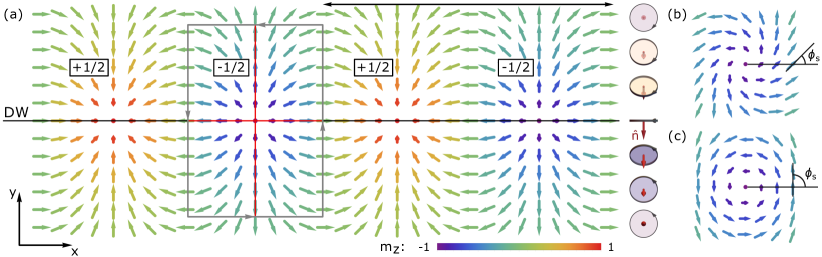
Figure 1: (a) Magnetization texture in the $xy$-plane associated with a meron DW parallel to the $xz$-plane (horizontal line). The texture is the same for every fixed $z$. Colors encode the magnetization component $m_{z}$. The upper domain is a clockwise spiral ($\chi=-1$) with the wave vector along $x$ (2). Across the DW, the spin rotation axis $\hat{n}$ rotates by 180^∘ (3) (right inset), leading to a counterclockwise spiral ($\chi=1$) in the lower domain. The gray contour encircles a meron with topological charge $\mathcal{Q}=-1/2$. In each spiral period, there are two merons with opposite topological charges. The perpendicular red lines show the two mirrors $m^{\prime}_{x,y}$ of merons. (b, c) Merons with helicity angles $\phi_{s}=\pi/4$ (b) and $\phi_{s}=\pi/2$ (c). The meron encircled in panel (a) has $\phi_{s}=0$. For $\phi_{s}\neq 0$, merons still have two discrete symmetries. However, these also involve a rotation in the $xy$-plane. We observe that $\phi_{s}$ determines the rotation axis of $\hat{n}$. For $\phi_{s}=0$, $\phi_{s}=\pi/4$ and $\phi_{s}=\pi/2$, $\hat{n}$ rotates around $\hat{x}$, $(\hat{x}+\hat{y})/\sqrt{2}$ and $\hat{y}$, respectively.

Meron domain wall structure. —

Let us consider the following Ginzburg-Landau Hamiltonian density describing a centrosymmetric cycloidal spiral magnet [16]

$$\mathcal{H} = J_{x}\left[-Q^{2}(\partial_{x}{\bf m})^{2}+\frac{1}{2}(\partial_{xx}^{2}{\bf m})^{2}\right]$$ (1)

$$+\frac{1}{2}\lvert J_{\perp}\rvert\left[(\partial_{y}{\bf m})^{2}+(\partial_{z}{\bf m})^{2}\right]+K_{z}m_{z}^{2},$$

where ${\bf m}({\bf r})$ denotes the magnetization direction and the lattice constant is set to $1$. The first term, proportional to $J_{x}>0$, promotes a spatial rotation of ${\bf m}({\bf r})$ with wave vector $\pm Q\hat{x}$. $J_{\perp}<0$ describes ferromagnetic interactions in the $yz$-planes. $K_{z}>0$ is an easy $xy$-plane anisotropy. Thus, the minimum energy configurations are two spirals in the $xy$-plane with opposite chirality $\chi=\pm 1$

$${\bf m}_{\chi}(x)=\left(\cos(Qx+\phi),\chi\sin(Qx+\phi),0\right),$$ (2)

where the constant phase $\phi$ corresponds to a translation of the whole spiral in the $x$-direction.

In the following, we consider the case where the region $y\ll\bar{y}$ has $\chi=+1$ (i.e. spin rotation axis $\hat{n}=\hat{z}$) and the region $y\gg\bar{y}$ has $\chi=-1$ (i.e. $\hat{n}=-\hat{z}$). Therefore, a DW parallel to the $xz$-plane with position $\bar{y}$ separates the two spiral domains (2). For simplicity, we assume that $J_{x}$ dominates (i.e. $K_{z}\ll J_{x}$ and $\lvert J_{\perp}\rvert\ll J_{x}$). To a first approximation, the lowest energy configuration minimizes the dominant term of the Hamiltonian density (1). Consequently, this configuration is a spiral with wave vector $Q$ for every fixed $y$. While moving from $y\ll\bar{y}$ to $y\gg\bar{y}$, the spin rotation axis $\hat{n}$ rotates from $\hat{z}$ to $-\hat{z}$ (see Fig. 1). Thus, the minimum energy configuration has the form

$${\bf m}(x,y)=\hat{\mathcal{R}}_{\hat{z}}(\phi_{s})\,\hat{\mathcal{R}}_{\hat{x}}\!\left(\theta(y-\bar{y})\right)\begin{pmatrix}\cos(Qx+\phi_{t})\\ \sin(Qx+\phi_{t})\\ 0\end{pmatrix},$$ (3)

where $\hat{\mathcal{R}}_{\hat{e}}(\alpha)$ is the rotation matrix around $\hat{e}$ by the angle $\alpha$. For $y\ll\bar{y}$ and $y\gg\bar{y}$, (3) reduces to the positive and negative chirality spirals (2) with $\phi\equiv\phi_{+}=\phi_{t}+\phi_{s}$ and $\phi\equiv\phi_{-}=\phi_{t}-\phi_{s}$. The function $\theta(y-\bar{y})$ is determined by minimizing the last two terms of the Hamiltonian (1) (see SI for details), resulting in

$$\hat{n}_{z}=\cos\theta(y-\bar{y})=-\tanh\!\left(\frac{y-\bar{y}}{\lambda_{0}}\right),$$ (4)

where $\lambda_{0}=\sqrt{\lvert J_{\perp}\rvert/2K_{z}}$ is the DW width. Therefore, a meron DW is simply a Bloch/Néel wall in $\hat{n}$ (see Fig. 1(a), right inset). The surface tension $\sigma=\sqrt{2K_{z}\lvert J_{\perp}\rvert}$ also resembles that of a DW in a ferromagnet with spin stiffness $J_{\perp}$ and easy axis anisotropy $K_{z}$.

The DW described by (3) and (4) consists of a periodic array of meron strings extending along $z$ and spaced by $\Delta x=\pi/Q$, in agreement with [16]. Figure 1 shows the magnetization texture in the $xy$-plane, which repeats for every fixed $z$. Inside the closed gray contour, ${\bf m}$ wraps the lower hemisphere, giving rise to a meron with topological charge $\mathcal{Q}=-1/2$. Such a meron has vorticity $n=1$ and helicity angle $\phi_{s}=0$. In fact, circulating counterclockwise around the meron string, ${\bf m}$ rotates by $2\pi$, and its projection on the $xy$-plane points along the radial direction close to the center. In general, the merons within the DW have the same vorticity $n=1$ but alternating topological charge $\mathcal{Q}=\pm 1/2$ and helicity angle $\varphi_{j}=\phi_{s}+\pi j$. If we reverse the domain chiralities, the meron vorticity becomes $n=-1$. We note that changes in $\phi_{s}$, $\phi_{t}$ and $\bar{y}$ correspond to rotations of ${\bf m}$ in the $xy$-plane, translations in the $x$-direction and translations in the $y$-direction, respectively. Thus, $\phi_{s}$, $\phi_{t}$ and $\bar{y}$ are the collective coordinates associated with the continuous symmetries of the Hamiltonian (1).

Our analysis concerns the DWs whose plane contains the spiral wave vector ${\bf Q}$. A wall with normal $\hat{e}_{\perp}$ forming an angle $\delta$ with ${\bf Q}$ presents two meron strings per spiral period spaced by $\pi/(Q\sin\delta)$, similar to vortex DWs [16]. Hence, only Hubert DWs (i.e. $\delta=0$) are meron-free, and we expect meron DW motion for $\delta=\pi/2$ to capture the essence of the dynamics for all other wall orientations.

Electric field-driven dynamics. —

Now we consider a DW in the presence of a uniform electric field ${\bf E}=E_{y}\hat{y}$. Inverse Dzyaloshinskii-Moriya effect that couples ${\bf E}$ and ${\bf m}$ is described by the Hamiltonian density [9, 8, 10]:

$$\mathcal{H}_{\mathrm{DM}}=-\gamma{\bf E}\cdot\left[({\bf m}\cdot\nabla){\bf m}-{\bf m}(\nabla\cdot{\bf m})\right].$$ (5)

Spiral domains with opposite chirality $\chi$ no longer have the same energy density because $\mathcal{H}_{\mathrm{DM}}=-\chi\gamma E_{y}Q$, and the favorable domain grows at the expense of the other, that is the meron DW moves in the $y$-direction.

The dynamics of magnetization is described by the following Lagrangian density and Rayleigh dissipation functional density [25, 26, 6]

$$\mathcal{L}={\bf A}({\bf m})\cdot\dot{{\bf m}}-\mathcal{H}_{\mathrm{tot}},\qquad\mathcal{R}=\frac{\alpha}{2}\dot{{\bf m}}^{2},$$ (6)

where ${\bf A}({\bf m})$ satisfies $\nabla_{\bf m}\times{\bf A}({\bf m})={\bf m}$, $\mathcal{H}_{\mathrm{tot}}=\mathcal{H}+\mathcal{H}_{\mathrm{DM}}$, $\alpha\ll 1$ is the Gilbert damping constant and the gyromagnetic ratio is set to $1$. The dynamics encoded in (6) can be solved for a magnetization field ${\bf m}(t,{\bf r})$ only in a few simple cases [1]. Therefore, we apply the collective coordinates approach instead [3, 4]. In such a framework, the dynamics is formulated in terms of collective coordinates $\xi_{I}(t)$, so that ${\bf m}(t,{\bf r})={\bf m}(\{\xi_{I}(t)\},{\bf r})$. Although ${\bf m}(t,{\bf r})$ has an infinite number of $\xi_{I}(t)$, only the soft modes with long relaxation times compared to the characteristic time of the dynamics are relevant. The other hard modes adjust adiabatically to their equilibrium values. In particular, the low-field (i.e. long time) dynamics is dominated by the zero modes corresponding to the continuous symmetries of the Hamiltonian (1), that is $\phi_{s}$, $\phi_{t}$ and $\bar{y}$.

From (6), descend the equations of motion for the collective coordinates [3, 4]

$$\alpha\Gamma_{IJ}\dot{\xi}_{J}-G_{IJ}\dot{\xi}_{J}=F_{I},$$ (7)

where $I$ and $J$ run over the soft modes, and the damping matrix $\Gamma_{IJ}=\Gamma_{JI}$, the gyrotropic matrix $G_{IJ}=-G_{JI}$ and the conservative forces $F_{I}$ acting on $\xi_{I}$ descend from $\mathcal{R}$, ${\bf A}({\bf m})\cdot\dot{{\bf m}}$ and $\mathcal{H}_{\mathrm{tot}}$, respectively (see SI for details).

The conservative forces due to the electric field $E_{y}$ are $F_{\bar{y}}=qE_{y}L_{x}L_{z}$, $F_{\phi_{s}}=F_{\phi_{t}}=0$, where $q=2Q\gamma$ is the electric charge density of the DW and the dimensions of the system are $L_{x}\times L_{y}\times L_{z}$. In the simplest case, where the wall contains an even number of merons with alternating topological charges $\mathcal{Q}_{i}$, $\bar{y}$ does not interact with $\phi_{s}$ and $\phi_{t}$. Indeed, $G_{\bar{y}\phi_{t}}=4\pi L_{z}\mathcal{Q}_{\mathrm{tot}}/Q$ is proportional to the total topological charge of the DW $\mathcal{Q}_{\mathrm{tot}}=\sum_{i}\mathcal{Q}_{i}=0$. (The general case $\mathcal{Q}_{\mathrm{tot}}\neq 0$ is discussed below.) The other components of $\Gamma_{IJ}$ and $G_{IJ}$ that couple $\bar{y}$ with $\phi_{s}$ and $\phi_{t}$ vanish for the mirror symmetries $m^{\prime}_{x,y}$ of the merons (see Fig. 1(a)). Therefore, $\phi_{s}$ and $\phi_{t}$ have a trivial dynamics, and, for the zero modes, (7) reduces to $\alpha\Gamma_{\bar{y}\bar{y}}\dot{\bar{y}}=F_{\bar{y}}$. All the previous results do not rely on the particular form of (3) and (4). Thus, they are expected to hold even beyond $K_{z}\ll J_{x}$ and $\lvert J_{\perp}\rvert\ll J_{x}$. Using (3) and (4), the damping constant of $\bar{y}$ reads $\alpha\Gamma_{\bar{y}\bar{y}}=\beta L_{x}L_{z}$, where $\beta=\alpha/\lambda_{0}$, and the DW velocity takes the form

$$\dot{\bar{y}}=Q\sqrt{\frac{2\lvert J_{\perp}\rvert}{K_{z}}}\frac{\gamma E_{y}}{\alpha}\equiv v_{\infty}.$$ (8)

At low electric fields, the long-time dynamics consists of the rigid translational motion of the DW with a constant velocity determined by the balance between the electric field and the dissipation. The system reaches this steady motion regime after a transient in which the hard modes adjust to their new equilibrium values. Nevertheless, at the first order in $E_{y}$, the steady-state velocity (8) is not affected by the presence of hard modes (see SI).

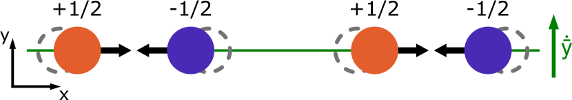
Figure 2: Meron DW moving with velocity $\dot{\bar{y}}$. The Lorentz-like gyrotropic force pushes oppositely charged merons in opposite directions, leading to dimerization.

To describe the transient dynamics, we need to include the momentum conjugate to $\bar{y}$, which it is coupled to via the gyrotropic matrix $G_{IJ}$. For a single meron, $G_{IJ}$ couples its translational modes along the $x$ and $y$ directions. Reparameterizing these modes in terms of the meron center $(\bar{x},\bar{y})$, we get $G_{\bar{x}\bar{y}}^{i}=4\pi L_{z}\mathcal{Q}_{i}$. Thus, considering each term in (7) as a force, the meron experiences a gyrotropic force ${\bf F}_{G}^{i}=4\pi L_{z}\mathcal{Q}_{i}\,[(\dot{\bar{x}},\dot{\bar{y}},0)\times\hat{z}]$ analogous to the Lorentz force [3]. In particular, as the wall moves with a velocity $\dot{\bar{y}}>0$, merons with positive $\mathcal{Q}_{i}$ are pushed to the right, while those with negative $\mathcal{Q}_{i}$ are pushed to the left, until ${\bf F}_{G}^{i}$ is balanced by the restoring force from $J_{x}$ in (1) (see Fig. 2). Hence, the meron DW dimerizes when it moves. Since this effect is due to the gyrotropic force, we expect the dimerization mode $d$ to have $G_{d\bar{y}}\neq 0$ and enter the effective Lagrangian as the momentum conjugate to $\bar{y}$.

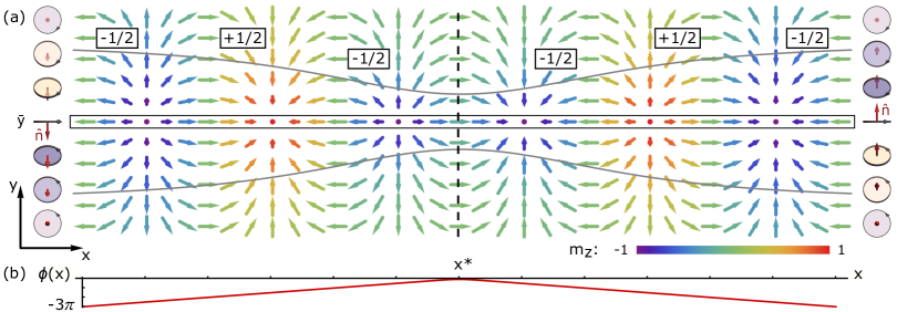
Figure 3: (a) Meron DW containing a defect. The topological charges are not alternating but have signature $\{...-+--+-...\}$. Hence, the total topological charge is $\mathcal{Q}_{\mathrm{tot}}=-1$. The dashed line indicates the defect plane $x=x^{*}$ that separates two regions where the spin rotation axis $\hat{n}$ rotates around $\hat{x}$ and $-\hat{x}$ (see side insets). The gray lines show the DW width $\lambda$ as a function of $x$. Near the defect, the DW is narrower in the $y$-direction. For $y=\bar{y}$ (black box), panel (b) represents the spiral phase $\phi(x)$ so that ${\bf m}(x,\bar{y})=\left(\cos\phi(x),0,\sin\phi(x)\right)$. A Hubert DW at $x=x^{*}$ separates the asymptotic regions $\partial_{x}\phi(x)=Q$ and $\partial_{x}\phi(x)=-Q$.

The alternating translations of merons along the $x$ direction representing dimerization can be incorporated in (3) via $\phi_{t}\rightarrow\phi_{t}+f(t,x,y-\bar{y}(t))$, where $f$ is determined by solving the variational problem of (6) (see SI). In the steady motion regime, $f$ has no explicit time dependence and $\bar{y}(t)=v_{\infty}t$. At the first order in $v_{\infty}$, we obtain

$$f(x,y-v_{\infty}t)=d_{\infty}\frac{\sin(Qx+\phi_{t})}{\cosh({(y-v_{\infty}t)/\lambda_{0}})},$$ (9)

where $d_{\infty}=mv_{\infty}$ determines dimerization in the steady motion regime and $m^{-1}=5J_{x}\lambda_{0}Q^{4}$. Replacing $d_{\infty}$ with $d(t)$ in (9) defines $f(t,x,y-\bar{y}(t))$ and therefore the dimerized configuration at time $t$ (see SI for an alternative definition). We observe that dimerization is associated with a net magnetic moment within the DW

$$\int{dV{\bf m}}=-\frac{\pi}{2}\lambda L_{x}L_{z}d\left(\cos\phi_{s},\sin\phi_{s},0\right),$$ (10)

which is the momentum conjugate to the rotations of ${\bf m}$ around $\hat{e}=\left(\cos\phi_{s},\sin\phi_{s},0\right)$. Such a rotation within the DW (3) corresponds to its motion in the $y$-direction.

At the first order in $E_{y}$, (7) takes the form

$$\begin{pmatrix}\beta&0\\ 0&\beta\lambda_{0}^{2}\end{pmatrix}\begin{pmatrix}\dot{\bar{y}}\\ \dot{d}\end{pmatrix}-\begin{pmatrix}0&-1\\ 1&0\end{pmatrix}\begin{pmatrix}\dot{\bar{y}}\\ \dot{d}\end{pmatrix}=\begin{pmatrix}qE_{y}\\ -d/m\end{pmatrix},$$ (11)

This equation descends from the effective Lagrangian and Rayleigh dissipation function

$$L=\dot{\bar{y}}d+qE_{y}\bar{y}-\frac{d^{2}}{2m},\qquad R=\frac{1}{2}\beta\dot{\bar{y}}^{2}+\frac{1}{2}\beta\lambda_{0}^{2}\dot{d}^{2}.$$ (12)

We observe that $d$ is the momentum conjugate to $\bar{y}$ (i.e. $d=\partial L/\partial\dot{\bar{y}}$), as anticipated.

Neglecting second-order terms in $\alpha\ll 1$ and assuming $\dot{\bar{y}}/v_{\infty}\gg\alpha^{2}$, the equations of motion (11) become

$$\dot{d}=m\ddot{\bar{y}}=qE_{y}-\beta\dot{\bar{y}},\qquad d=m\dot{\bar{y}}.$$ (13)

At low electric fields, the meron DW behaves as a particle with mass $m$, charge $q$ and viscous friction coefficient $\beta$. The dimerization mode plays the role of the momentum.

Solving (13) with the initial condition $\dot{\bar{y}}=v_{0}$ we get

$$\dot{\bar{y}}=v_{0}e^{-t/\tau}+v_{\infty}\left(1-e^{-t/\tau}\right),$$ (14)

where $\tau=m/\beta$ denotes the relaxation time of the dimerization mode $d(t)$, and $v_{\infty}$ is the steady-state velocity (8). Such a result captures both the transient and the steady motion regime. However, it cannot resolve the dynamics at timescales $t\ll\tau$ (e.g. the response to a pulse) because other modes may be active. In addition, at higher orders in $E_{y}$, DW deformations associated with hard modes may affect the dynamics. In particular, the effective mass and damping coefficient depend on the DW width $\lambda$. Hence, the high-field dynamics is sensible to the DW breathing mode that modulates $\lambda$.

We treat $\lambda$ as one of the collective coordinates by replacing $\lambda_{0}$ with $\lambda(t)$ in (4) and (9). Because (9) does not rely on the particular form of $v_{\infty}$, it continues to capture the dynamics up to the second order in the dimerization $d$ for $K_{z}\ll J_{x}$ and $\lvert J_{\perp}\rvert\ll J_{x}$. Neglecting second-order terms in $\alpha$, $\dot{d}$ and $\dot{\lambda}$, the equations of motion for $\bar{y}$, $d$ and $\lambda$ take the form (see SI for details)

$$m\frac{d}{dt}(\gamma_{c}\dot{\bar{y}})=qE_{y}-\beta\gamma_{c}\dot{\bar{y}},\quad d=m\gamma_{c}\dot{\bar{y}},\quad\lambda=\frac{\lambda_{0}}{\gamma_{c}},$$ (15)

where $\gamma_{c}^{-1}=\sqrt{1-\dot{\bar{y}}^{2}/c_{\mathrm{m}}^{2}}$, and $c_{\mathrm{m}}=\sqrt{5\lvert J_{\perp}\rvert J_{x}Q^{4}}$ is the DW limiting velocity. Remarkably, it coincides with the maximum magnon speed [27, 28, 29]. As the wall moves, its width is contracted by the Lorentz-like factor $\gamma_{c}$. Since $m,\beta\propto\lambda^{-1}$, they are multiplied by $\gamma_{c}$, leading to a “relativistic” DW dynamics, where $c_{\mathrm{m}}$ plays the role of the speed of light. Indeed, (13) goes into (15) through a substitution $\dot{\bar{y}}\rightarrow\gamma_{c}\dot{\bar{y}}$. The meron DW steady-state velocity corrected for the contraction of the wall width is

$$v_{\infty}^{\mathrm{rel}}=\frac{v_{\infty}}{\sqrt{1+v_{\infty}^{2}/c_{\mathrm{m}}^{2}}}<c_{\mathrm{m}}.$$ (16)

We corroborate the results with atomistic spin dynamics simulations [25, 26, 24] (see SI, Fig. S1, Fig. S2 and Movie 1). Meron DW structure and low-field dynamics are in excellent agreement with simulations. Furthermore, the high-field dynamics ($\dot{\bar{y}}\sim c_{\mathrm{m}}$) is recovered with periodic boundary conditions in the $x$-direction. Imposing open boundary conditions instead (exchange truncated at the boundaries), defect nucleation occurs at the surfaces when the DW velocity approaches $c_{\mathrm{m}}$ (see Fig. 3).

Defects within the meron wall. —

Equation (4) admits two solutions $\pm\theta(y-\bar{y})$ where the spin rotation axis $\hat{n}$ rotates in opposite directions. If solutions $\pm\theta$ are realized across a boundary $x=x^{*}$ lying between two merons (dashed line in Fig. 3), that leads to a low-energy defect within the DW, where two neighboring merons have the same topological charges $\mathcal{Q}_{i}=\mathcal{Q}_{i+1}$. This gives rise to a meron DW with non-alternating $\mathcal{Q}_{i}$ (e.g. with signature $\{...-+--+-\,...\}$, Fig. 3), in contrast to the previously considered minimum energy meron DW with alternating $\mathcal{Q}_{i}$ (i.e. $\{...+-+-\,...\}$, Fig. 1).

By relaxing a 2D paramagnetic state via the LLG dynamics [25, 26, 24] (see SI for details), we obtain several spiral domains (2), separated by meron DWs (see Fig. 4 and Fig. S3). Meron topological charges $\mathcal{Q}_{i}$ tend to alternate, but defects in this alternating order are also present (see Fig. 4(a)). Consequently, we expect these defects to exist in real systems, and studying how they affect the dynamics (even at low fields) is an essential problem.

Near a defect, the energy increases because the dominant term of the Hamiltonian density (1) (proportional to $J_{x}$) is not minimized (i.e., for a fixed $y$, the configuration is not a single spiral with wave vector $\pm Q$, see Fig. 3(b)). Consequently, merons shrink in the $y$-direction to reduce energy, decreasing the DW width $\lambda$. Since this effect is present only near the defects, $\lambda$ becomes a function of $x$ (see Fig. 3(a)). Far from the defects, $\lambda(x)$ asymptotically approaches the width of the minimum energy meron DW $\lambda_{0}=\sqrt{\lvert J_{\perp}\rvert/2K_{z}}$. Near the defects $\lambda(x)$ is smaller. For $K_{z}\ll J_{x}Q^{4}$, $\lambda\sim\sqrt{\lvert J_{\perp}\rvert/J_{x}Q^{4}}$. The $x$ dependence in $\lambda$ modifies $\Gamma_{\bar{y}\bar{y}}$ in $\Gamma_{\bar{y}\bar{y}}^{\prime}=L_{z}\int_{0}^{L_{x}}{dx/\lambda(x)}=b\Gamma_{\bar{y}\bar{y}}$, where the enhancement factor $b=(1/L_{x})\int_{0}^{L_{x}}{dx\>\lambda_{0}/\lambda(x)}$ is the average of $\lambda_{0}/\lambda(x)$ along the wall. Without defects, $b=1$, while in the presence of defects, the damping is enhanced by $b>1$. As the DW moves with velocity $\dot{\bar{y}}$, each meron experiences a damping force $F_{\Gamma}^{i}=-\alpha\Gamma_{\bar{y}\bar{y}}^{\prime i}\dot{\bar{y}}$. Since $\Gamma_{\bar{y}\bar{y}}^{\prime i}$ is larger near the defects, $F_{\Gamma}^{i}$ is non-uniform along the wall. This leads to a DW deformation so that the merons near the defects are falling behind (see SI, Fig. S4).

When the numbers of positive and negative defects are different, the DW has a net topological charge $\mathcal{Q}_{\mathrm{tot}}$, and $G_{\bar{y}\phi_{t}}=4\pi L_{z}\mathcal{Q}_{\mathrm{tot}}/Q\neq 0$. As the wall moves, $\phi_{t}$ experiences a force $-G_{\bar{y}\phi_{t}}\dot{\bar{y}}$ and $\phi_{s}$ – a force $-\alpha\Gamma_{\phi_{s}\phi_{t}}\dot{\phi}_{t}$. Thus, the magnetization rotates in the entire system unless $\phi_{t}$ and $\phi_{s}$ are pinned (e.g. by surface effects, anisotropy or disorder), a possibility we now neglect. Solving the equations of motion (7) for the zero modes $\phi_{s}$, $\phi_{t}$ and $\bar{y}$ (i.e. focusing on the low-field dynamics), we get

$$\dot{\bar{y}} = v_{\infty}\left(b+\frac{1}{\alpha^{2}}\frac{L_{y}\lambda_{0}}{\bar{y}(L_{y}-\bar{y})}\left(\frac{2\mathcal{Q}_{\mathrm{tot}}}{N}\right)^{2}\right)^{-1},$$

$$\dot{\phi}_{+} \equiv \dot{\phi}_{t}+\dot{\phi}_{s}=-\frac{2\mathcal{Q}_{\mathrm{tot}}}{N}\frac{\dot{\bar{y}}}{\alpha\bar{y}},$$

$$\dot{\phi}_{-} \equiv \dot{\phi}_{t}-\dot{\phi}_{s}=-\frac{2\mathcal{Q}_{\mathrm{tot}}}{N}\frac{\dot{\bar{y}}}{\alpha(L_{y}-\bar{y})},$$ (17)

where $N=L_{x}Q/\pi$ is the total number of merons within the DW, $\dot{\phi}_{+}$ and $\dot{\phi}_{-}$ are the precession speeds of ${\bf m}$ in the positive and negative chirality domains (2), respectively. As the wall moves, ${\bf m}$ rotates in each spiral domain, reducing the DW mobility by a factor that depends on its position $\bar{y}$ and total topological charge $\mathcal{Q}_{\mathrm{tot}}$. Such a non-local dynamics resemble that studied in Hubert DWs [5], which have $\mathcal{Q}_{\mathrm{tot}}=0$, but the origin is quite different. In fact, the meron DW position $\bar{y}$ and the spiral phases $\phi_{\pm}$ are three different zero modes coupled together (a Hubert DW instead has only two zero modes $\phi_{\pm}$). In particular, a meron DW can move even when $\phi_{\pm}$ are pinned, and ${\bf m}$ do not rotate in the entire system. Also, unlike a Hubert DW, the velocity of a meron DW with $\mathcal{Q}_{\mathrm{tot}}\neq 0$ reaches its maximum at the system center and goes to zero as it approaches the surfaces $y=0$ and $y=L_{y}$. We note that the result (17) holds in the bulk (i.e. $\lambda_{0}\ll\bar{y}\ll L_{y}-\lambda_{0}$), and surface effects are expected to prevent the wall from getting trapped inside the system (see SI, Fig. S5). Due to non-local dynamics, two distant DWs with net topological charges can affect each other’s motion (see SI for details). Hence, the DW velocities depend on the entire domain structure, similar to Hubert DWs.

Figure 4: Meron DW obtained by relaxing a paramagnetic configuration (see Fig. S3 for the entire domain structure, – Fig. 1 and Fig. 3 for the internal DW structure). Panels (a) and (b) show the topological charge density $\rho_{\mathrm{t}}={\bf m}\cdot\left[\partial_{x}{\bf m}\times\partial_{y}{\bf m}\right]/4\pi$ and the generalized chirality $\chi\equiv P_{y}/\gamma Q=\hat{z}\cdot\left[{\bf m}\times\partial_{x}{\bf m}\right]/Q$, respectively. Defects in the alternating charge order of merons correspond to regions where the wall is narrower. We observe that the DW has a net topological charge $\mathcal{Q}_{\mathrm{tot}}$ since the numbers of positive and negative defects are different.

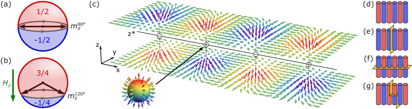
Figure 5: (a) Region of the sphere wrapped by a positive (red) and a negative (blue) meron for a DW separating two flat spiral domains. The magnetization in the domains map on the equator, resulting in the opposite meron topological charges $\pm 1/2$. (b) An out-of-plane magnetic field $H_{z}$ stabilizes the conical spiral with a conical angle $\vartheta_{c}=120^{\circ}$, leading to an imbalance between positive and negative merons. (c) Array of hedgehog defects with coordinates ${\bf x}_{j}=(x_{0}+j\pi/Q,\bar{y},z^{*})$ and alternating magnetic monopole charges connecting two half-spaces above and below $z=z^{*}$ where the meron topological charges have opposite signs. (d–g) Sketches of the meron strings (defect planes shown in yellow): (d) minimum energy DW (see Fig. 1); (e) defect between two meron strings (see Fig. 3); (f) array of point defects within the meron strings, corresponding to (c); (g) point defect within a single meron string. In the latter case, defect planes must also be present between the strings.

In the dynamics described by (17), merons translate in the $x$-direction with a velocity $\dot{\bar{x}}=-\dot{\phi}_{t}/Q\neq 0$. Therefore, merons are destroyed at one end of the wall, and new ones are created at the other (see Movies 2–4). Since the energy is higher when the boundary is cutting through a meron and lower when it is between two merons, such a process may affect the dynamics, exerting a force on $\phi_{t}$ and possibly exciting new modes. We study the effects of meron creation and destruction by performing numerical simulations (see SI, Fig. S5 and Movies 2–4). With open boundary conditions, the DW velocity oscillates around (17) with an amplitude proportional to the energy of created and destroyed merons. When a defect is destroyed, $\dot{\bar{y}}$ drops sharply, and $\mathcal{Q}_{\mathrm{tot}}$ changes because merons are created with alternating $\mathcal{Q}_{i}$. Except for these events, which occur on a short timescale compared to the characteristic time of the dynamics, (17) captures the averaged $\dot{\bar{y}}$ (see SI, Fig. S5). Consistently, ruling out meron creation and destruction by imposing periodic boundary conditions in the $x$-direction, simulations are in very good agreement with (17) for $\lambda_{0}\ll\bar{y}\ll L_{y}-\lambda_{0}$.

Topological charge control. —

An external magnetic field $H_{z}\hat{z}$ profoundly affects the dynamics of meron DWs. Indeed, $H_{z}$ induces a conical component in the spirals (2), which becomes ${\bf m}_{\chi}^{\vartheta_{c}}(x)=\sin\vartheta_{c}\,{\bf m}_{\chi}(x)+\cos\vartheta_{c}\,\hat{z}$, where $\vartheta_{c}\in(0,\pi)$ denotes the conical angle and $\vartheta_{c}=\pi/2$ gives a flat spiral (2) (see Fig. 5(a, b)). Adding the Zeeman term $\mathcal{H}_{\mathrm{Z}}=-\mu_{0}H_{z}m_{z}$ to the Hamiltonian (1) and minimizing the energy, we get

$$\cos\vartheta_{c}=\frac{\mu_{0}H_{z}}{2K_{z}+J_{x}Q^{4}}.$$ (18)

Within a positive meron, the polar angle $\vartheta$ varies between $0$ and $\vartheta_{c}$, while within a negative meron, $\vartheta\in(\vartheta_{c},\pi)$ (see Fig. 5(a, b)). Thus, the topological charges are

$$\mathcal{Q}_{+}=\frac{1-\cos\vartheta_{c}}{2},\qquad\mathcal{Q}_{-}=-\frac{1+\cos\vartheta_{c}}{2},$$ (19)

respectively, where $\cos\vartheta_{c}$ is given by (18). Therefore, $H_{z}$ changes the topological charge distribution of the wall. In particular, since $\mathcal{Q}_{+}$ and $\mathcal{Q}_{-}$ are no longer opposite, even a minimum energy DW has a net topological charge $\mathcal{Q}_{\mathrm{tot}}$ and exhibits a non-local dynamics. This is illustrated in Movie 5, where $H_{z}$ is turned on after the wall reaches the steady motion regime, leading to a substantial deceleration due to the precession of ${\bf m}$ in the entire system.

Helicity control. —

Within a meron DW, the magnetization components in the $xz$-plane induce a ferroelectric polarization in the $z$-direction. The average polarization due to the minimum energy DW is

$$P_{z}=-\frac{1}{V}\int{dV\>\frac{\partial\mathcal{H}_{\mathrm{DM}}}{\partial E_{z}}}=\frac{k}{L_{y}}\cos\phi_{s},$$ (20)

where $k=\pi\gamma(\lambda Q+1/2)$. Hence, the meron helicity angle $\phi_{s}$ determines $P_{z}$ and is sensitive to an external electric field $E_{z}$. The force exerted by $E_{z}$ on the minimum energy DW takes the form $F_{\phi_{s}}=-kE_{z}L_{x}L_{z}\sin\phi_{s}$. When $\phi_{t}$ is pinned (e.g. by surface effects) or does not interact with $\phi_{s}$ (i.e. the wall is at the center of the system $\bar{y}=L_{y}/2$), $\phi_{s}$ satisfies $\dot{\phi}_{s}=-(1/\tau_{s})\sin\phi_{s}$, where $\tau_{s}=\alpha L_{y}/kE_{z}$ has the same sign as $E_{z}$. The solution

$$P_{z}=\frac{k}{L_{y}}\tanh{\frac{t}{\tau_{s}}}$$ (21)

describes the switching of $P_{z}$ between $+k/L_{y}$ and $-k/L_{y}$ ($\phi_{s}$ between $0$ and $\pm\pi$) in an infinite time. Therefore, we expect the switching time of $P_{z}$ to be strongly influenced by fluctuations (e.g. thermal fluctuations).

Taking into account that $P_{z}$ is inverted across a defect plane (i.e. $\phi_{s}$ changes by $\pm\pi$), the result can be straightforwardly generalized to a meron DW with defects. Now, if $\bar{y}\neq L_{y}/2$ and $\mathcal{Q}_{\mathrm{tot}}\neq 0$, the DW moves under the action of $E_{z}$. Indeed, $E_{z}$ acts indirectly on $\bar{y}$ since the zero modes interact with each other.

Defects within meron strings. —

Up to this point, we have considered quasi-2D magnetization textures, where the meron DWs consist of an array of meron strings extending along $z$. Now, we study point defects within the meron strings. These are similar to the defects discussed above, but the solutions $\pm\theta$ are realized across a boundary $z=z^{*}$ instead of $x=x^{*}$ (see Fig. 5(c, f)). Hence, the topological charge of each meron string is reversed across the defect plane, leading to an array of point defects (one for each string) lying at the intersection of the defect and DW planes. Point defects are hedgehogs with alternating magnetic monopole charges since ${\bf m}$ wraps the upper and the lower hemisphere on opposite sides of $z=z^{*}$, and the meron helicities alternate within the wall. Meron strings do not carry net magnetic monopole charges since hedgehogs are compensated by charges arising at the intersections between strings and system surfaces. By relaxing a 3D paramagnetic state, configurations of this type arise naturally. A configuration with a single hedgehog can be realized by combining three defect planes $z=z^{*}$, $x=x^{*}$ and $x=x^{*}+\pi/Q$ (see Fig. 5(g)). The lengthscale of the hedgehogs is set by the lattice constant. Thus, point defects are strongly pinned to the lattice by Pierls-Nabarro barriers [30, 31], therefore pinning the meron DW.

Conclusions. —

We have shown that centrosymmetric spiral magnets exhibit DWs consisting of an array of meron strings, which result from the twisting of the spiral plane across the wall. The electric field-driven dynamics of meron DWs is intimately connected with the topology of the magnetization texture. The minimum energy walls contain merons with alternating topological charges. An applied electric field induces DW motion and alternating meron displacements along the array. This dimerization mode serves as the wall momentum and leads to inertia. The meron DW motion resembles that of a “relativistic” massive particle, with the magnon speed playing the role of the speed of light. Low-energy defects in the alternating charge sequence of merons appear during domain nucleation and can lead to DWs with net topological charge. Remarkably, this couples the motion of the wall to magnetization precession in the entire spiral domains, hence suppressing and making position-dependent the DW mobility. Fine control over such a non-local dynamics is enabled by an external magnetic field, which tunes the net topological charge of the DW. Meron helicity determines the out-of-plane polarization and can be easily manipulated by an external electric field. A Meron DW does not necessarily present a quasi-2D structure. Hedgehog point defects, analogous to Bloch points, separate the segments of a meron string with opposite topological charges, carry magnetic monopole charges, and pin the wall to the lattice. An interesting future direction is to explore how the topological charge (and thus magnetization) of individual merons can be modified by external magnetic fields. The motion of a hedgehog defect along the meron string may facilitate the topological charge switching. Consequently, meron DWs present a promising topologically protected computing platform in which topological charges provide natural binary variables associated with each meron.

Supplemental Information

I Meron domain wall structure: Energy minimization

Here we report the derivation of (4). Substituting the configuration (3) into the Hamiltonian density (1) we obtain

$$\mathcal{H}=\left(K_{z}\sin^{2}\!\theta-\frac{1}{2}J_{\perp}(\partial_{y}\theta)^{2}\right)\sin^{2}(Qx+\phi_{t})-\frac{1}{2}J_{x}Q^{4},$$ (S1)

where the constant contribution with $J_{x}$ is the lowest possible. Indeed, (3) minimizes the first term of the Hamiltonian density (1) by definition. Requiring $\delta H/\delta\theta=0$, where $H=\int{dV\>\mathcal{H}}$ and $\delta\cdot/\delta\theta$ denotes the functional derivative with respect to $\theta$, we get a stationary sine-Gordon equation for $\theta(y-\bar{y})$

$$J_{\perp}\partial_{yy}^{2}\theta+K_{z}\sin(2\theta)=0,$$ (S2)

where the boundary conditions are: $\theta\rightarrow 0$ for $y-\bar{y}\rightarrow-\infty$ and $\theta\rightarrow\pm\pi$ for $y-\bar{y}\rightarrow+\infty$ (i.e. $\chi=+1$ for $y\ll\bar{y}$ and $\chi=-1$ for $y\gg\bar{y}$). Multiplying by $\partial_{y}\theta$, (S2) can be rewritten as

$$\frac{1}{2}J_{\perp}(\partial_{y}\theta)^{2}+K_{z}\sin^{2}\!\theta=c,$$ (S3)

where the boundary conditions imply $c=0$. Hence, the equation for $\theta(y-\bar{y})$ takes the form

$$\lambda_{0}^{2}(\partial_{y}\theta)^{2}=\sin^{2}\!\theta,\qquad\qquad\lambda_{0}=\sqrt{\frac{\lvert J_{\perp}\rvert}{2K_{z}}}.$$ (S4)

The solutions satisfying the boundary conditions are

$$\theta_{\pm}(y-\bar{y})=\pm\arccos\!\left(\!\tanh\!\left(\!-\frac{y-\bar{y}}{\lambda_{0}}\right)\!\right),$$ (S5)

where we required $\theta_{\pm}(0)=\pm\pi/2$ (i.e. the DW has position $\bar{y}$).

II Electric field-driven dynamics: Zero modes

In this section, we derive $\Gamma_{IJ}$, $G_{IJ}$ and $F_{I}$ for a meron DW, focusing on the zero modes. Before starting, we briefly review the derivation of the equations of motion for the collective coordinates (7). Substituting ${\bf m}(t,{\bf r})={\bf m}(\{\xi_{I}(t)\},{\bf r})$ into (6) and integrating in space and time, one obtains the effective action functional $S$ and dissipation functional $D$

$$S\left[\{\xi_{I}(t)\}\right]=\int{dt\int{dV\left(\dot{\xi}_{J}{\bf A}({\bf m})\cdot\frac{\partial{\bf m}}{\partial\xi_{J}}-\mathcal{H}_{\mathrm{tot}}\right)}},\qquad\qquad D\left[\{\xi_{I}(t)\}\right]=\frac{\alpha}{2}\int{dt\int{dV\left(\dot{\xi}_{J}\frac{\partial{\bf m}}{\partial\xi_{J}}\right)^{\!2}}},$$ (S6)

where the dynamical variables are the collective coordinates $\xi_{I}(t)$. Requiring $\delta S/\delta\xi_{I}=\delta D/\delta\dot{\xi}_{I}$, one gets the equations of motion (7): $\alpha\Gamma_{IJ}\dot{\xi}_{J}-G_{IJ}\dot{\xi}_{J}=F_{I}$, where [3, 4]

$$\Gamma_{IJ}=\int{dV\>\frac{\partial{\bf m}}{\partial\xi_{I}}\cdot\frac{\partial{\bf m}}{\partial\xi_{J}}},\qquad\quad G_{IJ}=\int{dV\>{\bf m}\cdot\left[\frac{\partial{\bf m}}{\partial\xi_{I}}\times\frac{\partial{\bf m}}{\partial\xi_{J}}\right]},\qquad\quad F_{I}=-\int{dV\>\frac{\partial\mathcal{H}_{\mathrm{tot}}}{\partial\xi_{I}}}=-\frac{\partial H_{\mathrm{tot}}}{\partial\xi_{I}}.$$ (S7)

If $\xi_{I}(t)$ is a zero mode, $\partial\mathcal{H}/\partial\xi_{I}=0$ by definition and $F_{I}$ receive contributions only from $\mathcal{H}_{\mathrm{DM}}$ (5). In the presence of an electric field $E_{y}$, the DM energy density of the two spiral domains reads $\mathcal{H}_{\mathrm{DM}}=-\chi\gamma E_{y}Q$. Hence, a shift of the DW position $\Delta\bar{y}$ corresponds to $\Delta H_{\mathrm{DM}}=-2\gamma E_{y}QL_{x}L_{z}\Delta\bar{y}$, and the conservative force acting on $\bar{y}$ is $F_{\bar{y}}=2\gamma E_{y}QL_{x}L_{z}$. Instead, a rotation of ${\bf m}$ in the $xy$-plane or a translation in the $x$-direction does not change the size of the two spiral domains. Therefore, $\partial H_{\mathrm{DM}}/\partial\phi_{s}=\partial H_{\mathrm{DM}}/\partial\phi_{t}=0$ and $E_{y}$ exerts no force on $\phi_{s}$ and $\phi_{t}$.

We observe that $\partial_{\phi_{t}}=(1/Q)\partial_{x}$ and $\partial_{\bar{y}}=-\partial_{y}$. Consequently, $G_{\bar{y}\phi_{t}}$ can be rewritten as $G_{\bar{y}\phi_{t}}=4\pi L_{z}\mathcal{Q}_{\mathrm{tot}}/Q$, where

$$\mathcal{Q}_{\mathrm{tot}}=\frac{1}{4\pi}\int{dxdy\>{\bf m}\cdot\left[\partial_{x}{\bf m}\times\partial_{y}{\bf m}\right]}=\sum_{i}\mathcal{Q}_{i}$$ (S8)

is the total topological charge of the meron DW and $\mathcal{Q}_{i}$ denotes the topological charge of the $i$-th meron.

Since $\Gamma_{IJ}$ and $G_{IJ}$ are invariant under rotations of ${\bf m}$ (see (S7)), they are independent of $\phi_{s}$ and can be computed for $\phi_{s}=0$. In this case, the configuration (3) with the positive solution (S5) can be rewritten as

$${\bf m}(x^{\prime},y^{\prime})=(-\sin(Qx^{\prime}),-\sin\!\left(\Delta\theta(y^{\prime})\right)\cos(Qx^{\prime}),\cos\!\left(\Delta\theta(y^{\prime})\right)\cos(Qx^{\prime})),$$ (S9)

where we defined $x^{\prime}=x-\bar{x}=x+(\phi_{t}-\pi/2)/Q$, $y^{\prime}=y-\bar{y}$ and the odd function $\Delta\theta(y^{\prime})=\theta_{+}(y^{\prime})-\pi/2$. We note that $\mathcal{V}=(-\pi/2Q,\pi/2Q)\times(-l_{y},l_{y})\times(0,L_{z})$, where $l_{y}\sim\lambda_{0}$, corresponds to a single meron with center $(\bar{x},\bar{y})$. Both the magnetic texture (S9) and the DW region $\mathcal{V}$ are invariant under $\{x^{\prime}\rightarrow-x^{\prime},\,m_{x}\rightarrow-m_{x}\}$ and $\{y^{\prime}\rightarrow-y^{\prime},\,m_{y}\rightarrow-m_{y}\}$, but such symmetries act on the derivatives in the zero modes as follows:

$$\{x^{\prime}\rightarrow-x^{\prime},\,m_{x}\rightarrow-m_{x}\} :\qquad\partial_{\phi_{s}}\rightarrow-\partial_{\phi_{s}}, \qquad\partial_{\phi_{t}}\rightarrow-\partial_{\phi_{t}}, \qquad\partial_{\bar{y}}\rightarrow\partial_{\bar{y}}.$$ (S10)

$$\{y^{\prime}\rightarrow-y^{\prime},\,m_{y}\rightarrow-m_{y}\} :\qquad\partial_{\phi_{s}}\rightarrow-\partial_{\phi_{s}}, \qquad\partial_{\phi_{t}}\rightarrow\partial_{\phi_{t}}, \qquad\partial_{\bar{y}}\rightarrow-\partial_{\bar{y}}.$$

Therefore, every single meron gives no contributions to $\Gamma_{\bar{y}\phi_{s}}$, $\Gamma_{\bar{y}\phi_{t}}$ $G_{\bar{y}\phi_{s}}$, $\Gamma_{\phi_{t}\phi_{s}}$ and $G_{\phi_{t}\phi_{s}}$. Moreover, $\partial_{\bar{y}}{\bf m}$ is localized within the DW and the spiral domains also give no contributions to the first three. Thus, $\Gamma_{\bar{y}\phi_{s}}$, $\Gamma_{\bar{y}\phi_{t}}$ and $G_{\bar{y}\phi_{s}}$ vanish.

Assuming $\lambda_{0}\ll L_{y}$, the DW gives negligible contributions to $\Gamma_{\phi_{s}\phi_{s}}$, $\Gamma_{\phi_{t}\phi_{t}}$, $\Gamma_{\phi_{t}\phi_{s}}$ and $G_{\phi_{t}\phi_{s}}$. Therefore, we compute these components considering only the spiral domains. For $y-\bar{y}\ll-\lambda_{0}$ and $y-\bar{y}\gg\lambda_{0}$, the configuration (3) reduces to the positive and negative chirality spirals (2) with $\phi\equiv\phi_{+}=\phi_{t}+\phi_{s}$ and $\phi\equiv\phi_{-}=\phi_{t}-\phi_{s}$. Thus, we get

$$y\in(0,\bar{y}):\;\;\partial_{\phi_{s}}{\bf m}=\partial_{\phi_{t}}{\bf m},\qquad\qquad y\in(\bar{y},L_{y}):\;\;\partial_{\phi_{s}}{\bf m}=-\partial_{\phi_{t}}{\bf m},\qquad\qquad(\partial_{\phi_{s}}{\bf m})^{2}=(\partial_{\phi_{t}}{\bf m})^{2}=1.$$ (S11)

Combining (S7) and (S11), we obtain $\Gamma_{\phi_{s}\phi_{s}}=\Gamma_{\phi_{t}\phi_{t}}=L_{x}L_{y}L_{z}$, $\Gamma_{\phi_{t}\phi_{s}}=(2\bar{y}-L_{y})L_{x}L_{z}$ and $G_{\phi_{t}\phi_{s}}=0$.

To summarize the previous results, $\Gamma_{IJ}$, $G_{IJ}$ and $F_{I}$ take the form ($I,J=\phi_{s},\phi_{t},\bar{y}$)

$$\Gamma_{IJ}=\begin{pmatrix}L_{x}L_{y}&L_{x}(2\bar{y}-L_{y})&0\\ L_{x}(2\bar{y}-L_{y})&L_{x}L_{y}&0\\ 0&0&\Gamma_{\bar{y}\bar{y}}\end{pmatrix}\!L_{z},\quad G_{IJ}=\begin{pmatrix}\,0&0&0\\ \,0&0&-4\pi\mathcal{Q}_{\mathrm{tot}}/Q\\ \,0&4\pi\mathcal{Q}_{\mathrm{tot}}/Q&0\end{pmatrix}\!L_{z},\quad F_{I}=\begin{pmatrix}0\\ 0\\ 2\gamma E_{y}QL_{x}\end{pmatrix}\!L_{z},$$ (S12)

where $\Gamma_{\bar{y}\bar{y}}$ is the only component that depends on the internal structure of the meron DW. Using (3) and (4), we get $\Gamma_{\bar{y}\bar{y}}=L_{x}L_{z}/\lambda_{0}$. If the DW width $\lambda$ is a function of $x$, we obtain instead

$$\Gamma^{\prime}_{\bar{y}\bar{y}}=L_{z}\int_{0}^{L_{x}}\!{dx\>\frac{2\sin^{2}(Qx+\phi_{t})}{\lambda(x)}}\approx L_{z}\int_{0}^{L_{x}}\!{\frac{dx}{\lambda(x)}},$$ (S13)

where we assumed that $\lambda(x)$ is nearly constant in an interval $\Delta x=\pi/Q$ to replace $2\sin^{2}(Qx+\phi_{t})$ with the average.

Using these results, we obtain the long-time dynamics (8) and (17). At the first order in $E_{y}$, the hard modes do not affect such a dynamics. Let us consider a generic hard mode $h$ in the case of (8), that is, meron DWs with alternating $\mathcal{Q}_{i}$. In the steady motion regime, $\dot{h}=0$ and therefore the equation of motion (7) for $\bar{y}$ is still $\alpha\Gamma_{\bar{y}\bar{y}}\dot{\bar{y}}=F_{\bar{y}}$. However, $h$ stays in its equilibrium position $h_{\infty}(E_{y})$ and this corresponds to a deformation of the configuration (3). Thus, $\Gamma_{\bar{y}\bar{y}}$ and $F_{\bar{y}}$ may be modified. Nevertheless, the contribution to the previous equation is at least a second-order correction since $h_{\infty}(E_{y})$ is at least linear in $E_{y}$ (i.e. $h_{\infty}(0)=0$) and the equation has no zero-order term. Indeed, $\dot{\bar{y}}$ and $F_{\bar{y}}$ are both linear in $E_{y}$.

III Electric field-driven dynamics: Dimerization and breathing modes

As discussed in the main text, the dimerized meron DW at time $t$ takes the form

$${\bf m}(t,x,y)=\hat{\mathcal{R}}_{\hat{z}}(\phi_{s})\,\hat{\mathcal{R}}_{\hat{x}}\!\left(\theta(y-\bar{y}(t))\right)\begin{pmatrix}\cos(Qx+\phi_{t}+f(t,x,y-\bar{y}(t)))\\ \sin(Qx+\phi_{t}+f(t,x,y-\bar{y}(t)))\\ 0\end{pmatrix}.$$ (S14)

In the steady motion regime, $f$ has no explicit time dependence and $\bar{y}(t)=v_{\infty}t$ (i.e. $f(t,x,y-\bar{y}(t))\equiv f_{\infty}(x,y-v_{\infty}t)$). Substituting (S14) into (6) and requiring $\delta S/\delta f_{\infty}=\delta D/\delta\dot{f}_{\infty}$, where $S\left[f_{\infty}\right]=\int{dt\int{dV\>\mathcal{L}}}$ and $D\left[f_{\infty}\right]=\int{dt\int{dV\>\mathcal{R}}}$, we get the following equation for $f_{\infty}$ at the first order in $v_{\infty}$

$$\partial_{x}^{4}f_{\infty}(x,y-v_{\infty}t)-4Q^{2}\partial_{x}^{2}f_{\infty}(x,y-v_{\infty}t)=\frac{v_{\infty}}{J_{x}\lambda_{0}}\frac{\sin(Qx+\phi_{t})}{\cosh({(y-v_{\infty}t)/\lambda_{0}})},$$ (S15)

where we used $K_{z}\ll J_{x}$ and $\lvert J_{\perp}\rvert\ll J_{x}$. Seeking a solution of the form $f_{\infty}(x,y-v_{\infty}t)=\sin(Qx+\phi_{t})\,g(y-v_{\infty}t)$, we obtain (9). Then, promoting $d_{\infty}$ to $d(t)$, $f$ takes the form

$$f(t,x,y-\bar{y}(t))=d(t)\frac{\sin(Qx+\phi_{t})}{\cosh({(y-\bar{y}(t))/\lambda_{0}})}.$$ (S16)

Above, we defined the dimerized configuration in the transient from that in the steady motion regime. It is possible to give an alternative (but equivalent) definition, based on the action of $E_{y}$ at the initial time $t=0$. The magnetization field ${\bf m}(t,{\bf r})$ obeys the LLG equation [25, 26], obtained from (6) as ${\bf m}\times(\delta S/\delta{\bf m}-\delta D/\delta\dot{{\bf m}})=0$,

$$\dot{{\bf m}}={\bf m}\times\frac{\delta H_{\mathrm{tot}}}{\delta{\bf m}}+\alpha\,{\bf m}\times\dot{{\bf m}}.$$ (S17)

In particular, the contribution of the electric field $E_{y}$ reads $(\dot{{\bf m}})_{\mathrm{DM}}={\bf m}\times\delta H_{\mathrm{DM}}/\delta{\bf m}=2\gamma E_{y}\,{\bf m}\times[\hat{z}\times\partial_{x}{\bf m}]$. After a short time interval $\Delta t$, the meron DW is deformed: ${\bf m}(\Delta t,{\bf r})\approx{\bf m}(0,{\bf r})+(\dot{{\bf m}})_{\mathrm{DM}}\Delta t$, where we neglected the dissipation. Using the static magnetization texture (3) (i.e. the configuration at the initial time), we get $(\dot{{\bf m}})_{\mathrm{DM}}\cdot\partial_{\bar{y}}{\bf m}=0$. Hence, such a deformation does not involve $\bar{y}$ but another collective coordinate $d$ so that

$${\bf m}(t,x,y)={\bf m}(0,x,y)-\frac{d(t)}{Q}\,{\bf m}(0,x,y)\times\left[\hat{z}\times\partial_{x}{\bf m}(0,x,y)\right],$$ (S18)

where the factor $-1/Q$ is added for convenience, and ${\bf m}(0,x,y)$ is given by (3) and (4). The previous equation defines the dimerized configuration at the first order in $d$ and, consistently, it coincides with the first order expansion of (S14) and (S16). The fact that the driving force does not act directly on the DW position but only changes $d$ corroborates the identification of the dimerization mode with the momentum conjugate to $\bar{y}$.

To derive (S14) and (S16), we did not use the explicit forms of $\lambda_{0}$ and $v_{\infty}$. Thus, these are true even at high electric fields, when $\lambda_{0}\rightarrow\lambda(t)$ and the steady velocity differs from (8). Up to the second order in $d$, (7) takes the form

$$\frac{\alpha}{\lambda_{0}}\begin{pmatrix}\gamma_{c}&0&0\\ 0&\lambda_{0}^{2}/\gamma_{c}&d\lambda_{0}/2\\ 0&d\lambda_{0}/2&\gamma_{c}\pi^{2}/12\end{pmatrix}\begin{pmatrix}\dot{\bar{y}}\\ \dot{d}\\ \dot{\lambda}\end{pmatrix}-\begin{pmatrix}0&-1&0\\ 1&0&0\\ 0&0&0\end{pmatrix}\begin{pmatrix}\dot{\bar{y}}\\ \dot{d}\\ \dot{\lambda}\end{pmatrix}=\begin{pmatrix}qE_{y}\\ -d/m\gamma_{c}\\ -K_{z}\left(1-\gamma_{c}^{2}+d^{2}/m^{2}c^{2}_{\mathrm{m}}\right)\end{pmatrix},$$ (S19)

where $\gamma_{c}=\lambda_{0}/\lambda$, $q=2Q\gamma$, $m^{-1}=5J_{x}\lambda_{0}Q^{4}$, $c_{\mathrm{m}}=\sqrt{5\lvert J_{\perp}\rvert J_{x}Q^{4}}$, and the second-order corrections of $f(t,x,y-\bar{y}(t))$ do not contribute for $K_{z}\ll J_{x}$ and $\lvert J_{\perp}\rvert\ll J_{x}$. Neglecting second-order terms in $\alpha$, $\dot{d}$ and $\dot{\lambda}$, (S19) becomes

$$\dot{d}=qE_{y}-\beta\gamma_{c}\dot{\bar{y}},\qquad d=m\gamma_{c}\dot{\bar{y}},\qquad\gamma_{c}=\frac{1}{\sqrt{1-\dot{\bar{y}}^{2}/c^{2}_{\mathrm{m}}}},$$ (S20)

where $\beta=\alpha/\lambda_{0}$, and $\gamma_{c}$ resembles the Lorentz factor with $c_{\mathrm{m}}$ playing the role of the speed of light.

IV Defects within the meron wall: Dynamics of multiple domain walls

Let us consider $K$ meron DWs with positions $\bar{y}_{k}$, which separate $K+1$ spiral domains with phases $\phi_{k}$ and alternating chiralities $\chi_{k}$. For $I=\phi_{k}$, the equations of motion (7) express the precession speed of ${\bf m}$ in the $k$-th domain in terms of the velocities of the adjacent DWs:

$$\dot{\phi}_{k}=-\frac{2}{\alpha N}\frac{\mathcal{Q}_{k}\dot{\bar{y}}_{k}+\mathcal{Q}_{k-1}\dot{\bar{y}}_{k-1}}{\bar{y}_{k}-\bar{y}_{k-1}},$$ (S21)

where $N=L_{x}Q/\pi$ is the total number of merons within a single DW, $\mathcal{Q}_{k}$ denotes the total topological charge of the $k$-th wall, $\bar{y}_{0}\equiv 0$, $\bar{y}_{K+1}\equiv L_{y}$ and $\dot{\bar{y}}_{0}=\dot{\bar{y}}_{K+1}\equiv 0$ are defined to simplify the notation. For $I=\bar{y}_{k}$ with $k=1,2,\ldots,K$, the equations of motion (7) thus take the form

$$\begin{pmatrix}C_{11}&C_{12}&0&0&\cdots\\ C_{12}&C_{22}&C_{23}&0&\cdots\\ 0&C_{23}&C_{33}&C_{34}&\cdots\\ 0&0&C_{34}&C_{44}&\mathclap{\smash{\ddots}}\\ \vdots&\vdots&\vdots&\mathclap{\smash{\ddots}}&\mathclap{\smash{\ddots}}\end{pmatrix}\begin{pmatrix}\dot{\bar{y}}_{1}\\ \dot{\bar{y}}_{2}\\ \dot{\bar{y}}_{3}\\ \dot{\bar{y}}_{4}\\ \vdots\end{pmatrix}=\begin{pmatrix}\pm v_{\infty}\\ \mp v_{\infty}\\ \pm v_{\infty}\\ \mp v_{\infty}\\ \vdots\end{pmatrix},$$ (S22)

where upper and lower signs in front of $v_{\infty}$ (8) correspond to the cases in which the first domain has chirality $\chi_{1}=+1$ and $\chi_{1}=-1$, respectively, and

$$C_{kk}=b_{k}+\frac{\lambda_{0}}{\alpha^{2}}\frac{\bar{y}_{k+1}-\bar{y}_{k-1}}{(\bar{y}_{k}-\bar{y}_{k-1})(\bar{y}_{k+1}-\bar{y}_{k})}\left(\frac{2\mathcal{Q}_{k}}{N}\right)^{2},\qquad C_{kl}=C_{lk}=\frac{\lambda_{0}}{\alpha^{2}}\frac{1}{\lvert\bar{y}_{k}-\bar{y}_{l}\rvert}\frac{4\mathcal{Q}_{k}\mathcal{Q}_{l}}{N^{2}}\quad\mathrm{for}\ \lvert k-l\rvert=1.$$ (S23)

The $k$-th DW exerts a force $F_{kl}\propto C_{kl}\dot{\bar{y}}_{k}$ on the neighboring walls (labeled by $l$). Since $C_{kl}$ is proportional to $\mathcal{Q}_{k}$ and $\mathcal{Q}_{l}$, a meron DW with zero total topological charge does not interact with the others.

V Atomistic spin dynamics simulations

To support the analytical results, we perform various atomistic spin dynamics simulations using the UppASD code [24], which numerically solves the LLG equation (S17). Since the $z$-coordinate plays no role, we consider the following 2D discrete model

$$H=\sum_{\bf r}\left(J_{1}\,{\bf S}_{\bf r}\cdot{\bf S}_{{\bf r}+\hat{x}}+J_{2}\,{\bf S}_{\bf r}\cdot{\bf S}_{{\bf r}+2\hat{x}}+J_{\perp}\,{\bf S}_{\bf r}\cdot{\bf S}_{{\bf r}+\hat{y}}+K_{z}\left({\bf S}_{\bf r}\cdot\hat{z}\right)^{2}-\gamma E_{y}\hat{z}\cdot\left[{\bf S}_{\bf r}\times{\bf S}_{{\bf r}+\hat{x}}\right]\right)$$ (S24)

with competing nearest neighbor $J_{1}<0$ and next nearest neighbor $J_{2}>0$ exchange interactions in the $x$-direction, ferromagnetic $J_{\perp}<0$ in the $y$-direction, easy $xy$-plane anisotropy $K_{z}>0$ and DM vector $-\gamma E_{y}\hat{z}$. For ${\pi/Q\gg 1}$ and ${\lambda_{0}\gg 1}$, the Hamiltonian (S24) is equivalent to the spatial integral of $\mathcal{H}_{\mathrm{tot}}$ (see (1) and (5)) with $J_{x}=J_{2}\sin^{2}\!Q/Q^{2}$ and $Q=\arccos(-J_{1}/4J_{2})$.

We simulate a $60\times 90$ system with periodic boundary conditions in the $x$-direction and open boundary conditions in the $y$-direction. The magnetic moment magnitude of a site is set to the Bohr magneton $\mu_{B}$. In the first simulation, we choose $J_{1}=-1.4\;\mathrm{mRy}$, $J_{2}=0.38\;\mathrm{mRy}$, $J_{\perp}=-0.1\;\mathrm{mRy}$, $K_{z}=0.002\;\mathrm{mRy}$, $\gamma E_{y}=0.0002\;\mathrm{mRy}$, $\alpha=0.1$, the time-step $\delta t=3\cdot 10^{-16}\,\mathrm{s}$ and the total number of iterations $\mathcal{N}=6\cdot 10^{5}$. The initial state is the minimum energy DW (3) corresponding to $J_{1}$, $J_{2}$, $J_{\perp}$ and $K_{z}$. Restoring the lattice constant $a=5\cdot 10^{-10}\,\mathrm{m}$, the magnetization magnitude $\lvert m\rvert=\mu_{B}/a^{3}$ and the gyromagnetic ratio $\gamma_{g}=g\mu_{B}/\hbar$, where $g=2$, we get

$$\mathrm{Analytical:} \qquad v_{\infty}=173\;\mathrm{m/s}, \qquad\tau=4.35\cdot 10^{-12}\,\mathrm{s}, \qquad d_{\infty}=0.030,$$ (S25)

$$\mathrm{Simulation:} \qquad v_{\infty}=167\;\mathrm{m/s}, \qquad\tau=4.89\cdot 10^{-12}\,\mathrm{s}, \qquad d_{\infty}=0.033,$$

where $\tau$ denotes the relaxation time of the dimerization mode, $v_{\infty}$ and $d_{\infty}$ are the steady-state velocity and dimerization. The discrepancies are $3.6\%$, $12\%$ and $10\%$, respectively. To further corroborate the analytical model, we perform various simulations, changing $J_{2}$, $J_{\perp}$, $K_{z}$ and $\alpha$ one by one. Figure S2 shows the results and the fit of $\dot{\bar{y}}(t)$ (14) that determines $v_{\infty}$ and $\tau$. Instead, $d_{\infty}$ is obtained by fitting the configuration described by (S14), (S5) and (S16) to the magnetization texture observed in simulations (see Fig. S1). In order to better visualize dimerization in Fig. S1 and Movie 1, we enhance it by choosing a different set of parameters: $J_{1}=-1.52\;\mathrm{mRy}$, $J_{2}=0.4\;\mathrm{mRy}$, $J_{\perp}=-0.1\;\mathrm{mRy}$, $K_{z}=0.004\;\mathrm{mRy}$, $\gamma E_{y}=0.002\;\mathrm{mRy}$. Still, the values for the dimerization from analytical and numerical calculations, $d_{\infty}=0.67$ and $d_{\infty}=0.62$, are in good agreement.

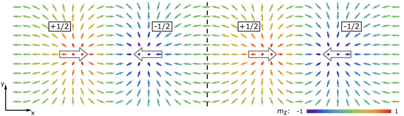
Figure S1: Meron DW moving under the action of an applied electric field $E_{y}$. Gray arrows highlight dimerization (i.e. alternating meron displacements). The dashed line separates the magnetization texture observed in the simulation (left) and the analytical solution with fitted $\phi_{s}$, $\phi_{t}$, $\bar{y}$ and $d$ (right).

We repeat the simulation (S25) using open (instead of periodic) boundary conditions in the $x$-direction, which may be a more realistic setup. The initial configuration is numerically relaxed before the electric field $E_{y}$ is applied. The fit of $\dot{\bar{y}}(t)$ (14) is still good, and the resulting steady velocity and transient time are $v_{\infty}=149\;\mathrm{m/s}$ and $\tau=5.57\cdot 10^{-12}\,\mathrm{s}$. Since the magnetization texture is deformed near the surfaces, we restrict the fit of (S14) to the central region of the DW, obtaining $d_{\infty}=0.034$. Increasing $L_{x}$ from $60$ to $150$, we get $v_{\infty}=161\;\mathrm{m/s}$, $\tau=5.21\cdot 10^{-12}\,\mathrm{s}$ and $d_{\infty}=0.034$, which are in better agreement with (S25). The larger the system, the less relevant the surface effects are. Hence, for $L_{x}\gg\pi/Q$, we expect to recover (S25).

To test the “relativistic” DW dynamics (15) and (16), we run several simulations of a $60\times 500$ system with periodic boundary conditions in the $x$-direction, open boundary conditions in the $y$-direction and parameters: $J_{1}=-1.4\;\mathrm{mRy}$, $J_{2}=0.38\;\mathrm{mRy}$, $J_{\perp}=-0.1\;\mathrm{mRy}$, $K_{z}=0.001\;\mathrm{mRy}$, $\alpha=0.005$ and $\gamma E_{y}\in(2.5\cdot 10^{-6},\,4\cdot 10^{-4})\,\mathrm{mRy}$. We obtain

$$\mathrm{Analytical:} \qquad c_{\mathrm{m}}=1541\;\mathrm{m/s}, \qquad\mu_{\mathrm{DW}}=2.45\cdot 10^{7}\,\mathrm{m/(s\,mRy)},$$ (S26)

$$\mathrm{Simulations:} \qquad c_{\mathrm{m}}=1450\;\mathrm{m/s}, \qquad\mu_{\mathrm{DW}}=2.36\cdot 10^{7}\,\mathrm{m/(s\,mRy)},$$

where $c_{\mathrm{m}}$ is the limiting velocity, and $\mu_{\mathrm{DW}}=v_{\infty}/\gamma E_{y}$ denotes the low-field DW mobility. The discrepancies are $6.1\%$ and $3.7\%$, respectively. Figure S2(f) shows the fit of (16) that determines (S26).

We simulate a $120\times 120$ system with open boundary conditions and parameters: $J_{1}=-1.08\;\mathrm{mRy}$, $J_{2}=0.38\;\mathrm{mRy}$, $J_{\perp}=-0.1\;\mathrm{mRy}$, $K_{z}=0.002\;\mathrm{mRy}$, $\alpha=0.1$, $\delta t=2\cdot 10^{-16}\,\mathrm{s}$ and $\mathcal{N}=4\cdot 10^{5}$. The electric field $E_{y}$ is now set to $0$, and the initial configuration is random (i.e. each spin points in a random direction). The resulting magnetization texture consists of four spiral domains (two with $\chi=+1$ and two with $\chi=-1$) separated by three meron DWs with defects, two of which have $\mathcal{Q}_{\mathrm{tot}}\neq 0$ (see Fig. S3). This confirms that defects within the meron chain are metastable and can lead to DWs with a non-zero total topological charge. We observe that the conditions required to obtain only meron DWs by relaxing a random configuration are stricter than DW metastability. For example, if $J_{1}=-1.4\;\mathrm{mRy}$, meron DWs are metastable (i.e. by relaxing the configuration (3), only negligible corrections in $K_{z}$ and $J_{\perp}$ appear), but the simulation where a random configuration is relaxed does not result in meron DWs. For this to happen, meron DWs must be much lower in energy than any other DW type. In particular, considering the competition with Hubert DWs, such a condition takes the form $L_{x}\sqrt{K_{z}\lvert J_{\perp}\rvert}\ll L_{y}J_{2}Q\sin^{2}\!Q$, where $a$ is set to $1$. Therefore, we can compensate for the increase in $\lvert J_{1}\rvert$ (i.e. the decrease in $Q$) by increasing $L_{y}/L_{x}$.

In order to simulate the dynamics of meron DWs with defects, we proceed similarly to the case of minimum energy DWs. The main difference is that now we can not rely on the analytical expression for the DW structure to create the initial configuration because $\lambda(x)$ is unknown. Hence, we invert $m_{z}$ within a few merons in (3) and then numerically relax the configuration. As discussed in the main text, the damping force $F_{\Gamma}^{i}$ is stronger near the defects. Consistently, in simulations, the merons near the defects are falling behind (see Fig. S4). The collective coordinate corresponding to this deformation is a hard mode. Thus, we neglect it in the derivation of the long-time dynamics (17). In addition, we consider a DW where all the merons have the same topological charge (see Fig. S5 and Movie 2). The simulation clearly shows bulk rotations of spins and agrees with (17) far from the surfaces $y=0$ and $y=L_{y}$. Still, the analytical model, which does not take surface effects into account, fails to describe the near-surface behavior. Indeed, it predicts that the DW velocity $\dot{\bar{y}}$ goes to zero at the surfaces, while in the simulation $\dot{\bar{y}}$ increases sharply due to open boundary conditions in the $y$-direction. In the above simulation, the boundary conditions in the $x$-direction are periodic. Using open boundary conditions instead, the dynamics changes significantly. Bulk rotations of spins are still observed, but only above a critical electric field. Indeed, the driving field must overcome an energy barrier to push a meron through the boundary and activate $\phi_{t}$. Moreover, the destruction of a defect at one end of the wall (see Movie 3) corresponds to a drop in the velocity $\dot{\bar{y}}$ (see Fig. S5, right side), which is not described by (17). Since merons created at the other end have alternating topological charges (see Movie 3), $\mathcal{Q}_{\mathrm{tot}}$ reduces as the DW moves. Instead, when the destroyed merons have alternating topological charges (see Movie 4), the velocity $\dot{\bar{y}}$ oscillates around (17) (see Fig. S5, left side), and $\mathcal{Q}_{\mathrm{tot}}$ remains the same. Hence, the analytical solution (17) captures the averaged DW velocity.

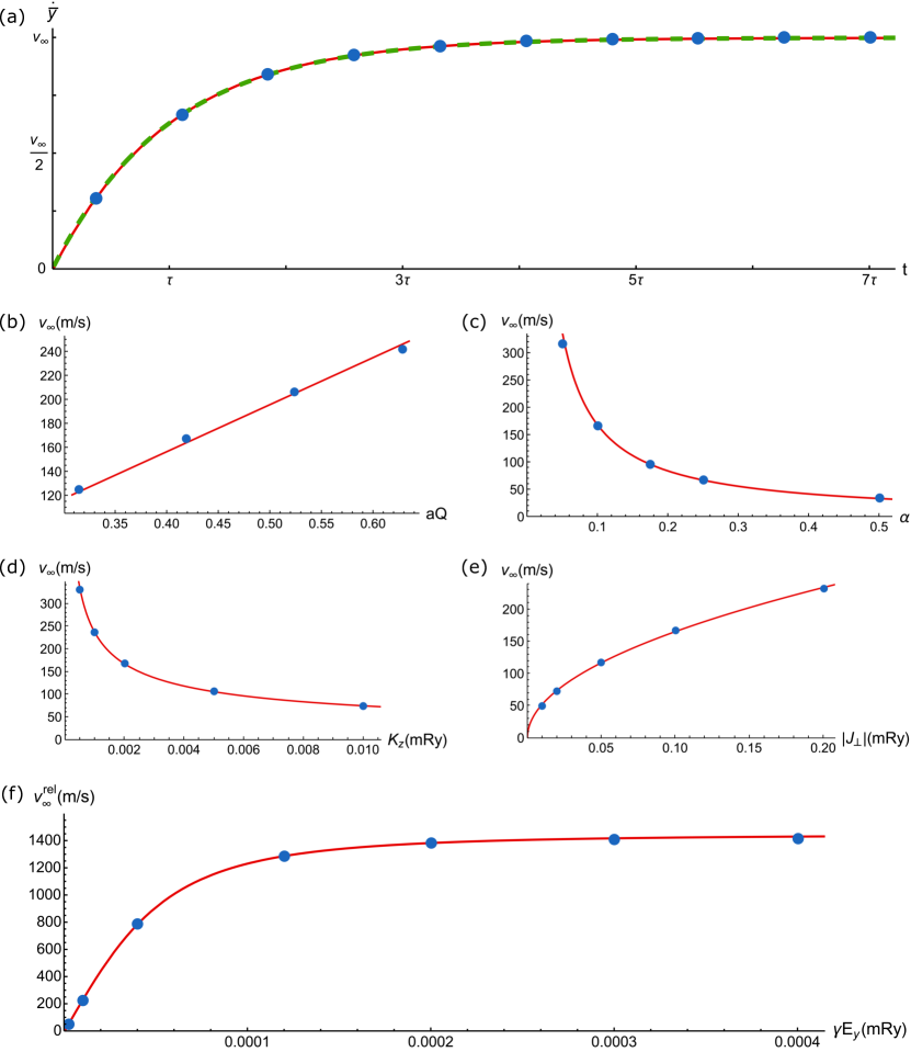
Figure S2: (a) Meron DW velocity as a function of time. The green and red lines represent the numerical result and the analytical solution (14) with fitted $v_{\infty}$ and $\tau$ (here $v_{0}=0$). The Blue dots indicate $d/m$ as a function of $t$. The dimerization $d$ is obtained by fitting the configuration given by (S14), (S5) and (S16) to the magnetization texture observed in simulations. The effective mass $m$ is determined by averaging the numerical $d/\dot{\bar{y}}$ (see (13)). Panels (b), (c), (d), (e) and (f) show the DW steady velocity as a function of $aQ$, $\alpha$, $K_{z}$, $\lvert J_{\perp}\rvert$ and $\gamma E_{y}$, respectively. The blue dots indicate the numerical results, and the red lines represent the fitted analytical solutions (8) and (16).

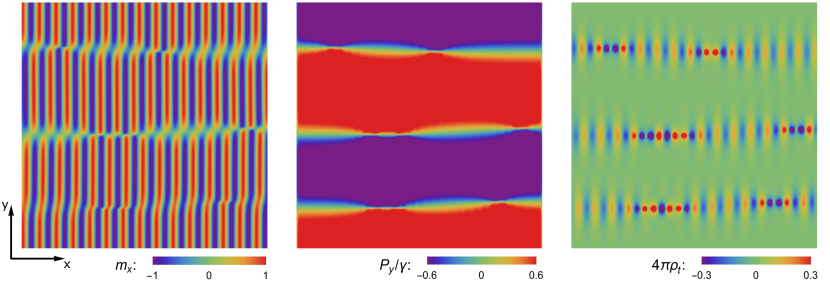
Figure S3: Magnetization texture obtained by relaxing a random configuration. From left to right, the density plots represent the magnetization $x$-component $m_{x}$, the (re-scaled) polarization $y$-component $P_{y}/\gamma$ and the (re-scaled) topological charge density $4\pi\rho_{t}$. Three meron DWs with defects separate four spiral domains. From $P_{y}/\gamma$ and $4\pi\rho_{t}$ it is clear that the walls are narrower near the defects. Furthermore, the two lower DWs have a non-zero total topological charge.

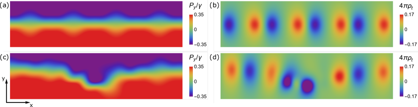
Figure S4: Minimum energy DW (a),(b) and defected DW with $\mathcal{Q}_{\mathrm{tot}}=0$ (c),(d) moving under the action of $E_{y}$. The left panels show the (re-scaled) polarization $y$-component $P_{y}/\gamma$. The right panels represent the (re-scaled) topological charge density $4\pi\rho_{t}$. Merons near the defect are falling behind, and the DW is deformed.

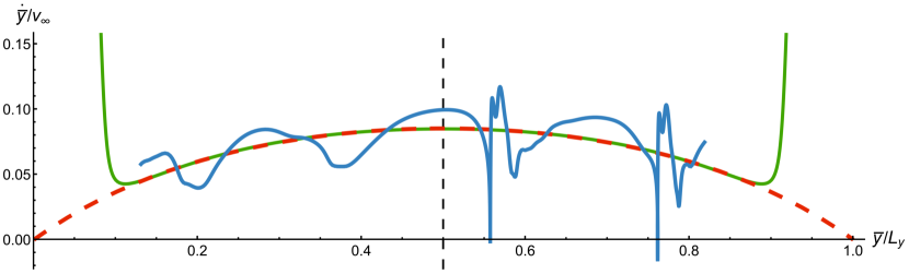
Figure S5: Velocity of a meron DW with $\mathcal{Q}_{\mathrm{tot}}\neq 0$ as a function of its position. The green and red lines indicate the numerical result with periodic boundary conditions in the $x$-direction and the analytical solution (17) with fitted parameters. Because of open boundary conditions in the $y$-direction, the surface attracts the DW when the distance between the two is comparable to the wall width. Equation (17) does not take this effect into account. The blue line represents a simulation with open boundary conditions in the $x$-direction. In the graphic left half, merons with alternating topological charges are destroyed, and $\dot{\bar{y}}$ oscillates around (17) (red line). In the right half, two defects are destroyed, and $\dot{\bar{y}}$ drops sharply at these events.

References

- Schryer and Walker [1974] N. L. Schryer and L. R. Walker, J. Appl. Phys. 45, 5406 (1974).
- Thiele [1973] A. A. Thiele, Phys. Rev. Lett. 30, 230 (1973).
- Tretiakov et al. [2008] O. A. Tretiakov, D. Clarke, G.-W. Chern, Y. B. Bazaliy, and O. Tchernyshyov, Phys. Rev. Lett. 100, 127204 (2008).
- Clarke et al. [2008] D. J. Clarke, O. A. Tretiakov, G.-W. Chern, Y. B. Bazaliy, and O. Tchernyshyov, Phys. Rev. B 78, 134412 (2008).
- Foggetti et al. [2024] F. Foggetti, M. Parodi, N. Nagaosa, and S. Artyukhin, Electric field-induced domain wall motion in spin spiral multiferroics (2024), arXiv:2204.09027 [cond-mat.str-el] .
- Duine [2010] R. A. Duine, Lecture notes on spintronics (2010).
- Kimura et al. [2003] T. Kimura, T. Goto, H. Shintani, K. Ishizaka, T.-h. Arima, and Y. Tokura, Nature 426, 55 (2003).
- Katsura et al. [2005] H. Katsura, N. Nagaosa, and A. V. Balatsky, Phys. Rev. Lett. 95, 057205 (2005).
- Mostovoy [2006] M. Mostovoy, Phys. Rev. Lett. 96, 067601 (2006).
- Sergienko and Dagotto [2006] I. A. Sergienko and E. Dagotto, Phys. Rev. B 73, 094434 (2006).
- Cheong and Mostovoy [2007] S. W. Cheong and M. Mostovoy, Nature Mater. 6, 13 (2007).
- Roy et al. [2012] A. Roy, R. Gupta, and A. Garg, Advances in Condensed Matter Physics 2012, 926290 (2012).
- Polyakov and Belavin [1975] A. M. Polyakov and A. A. Belavin, JETP Lett. 22, 245 (1975).
- Bogdanov and Hubert [1994] A. Bogdanov and A. Hubert, Journal of Magnetism and Magnetic Materials 138, 255 (1994).
- Mostovoy [2023] M. Mostovoy, Journal of the Physical Society of Japan 92, 081005 (2023).
- Li et al. [2012] F. Li, T. Nattermann, and V. L. Pokrovsky, Phys. Rev. Lett. 108, 107203 (2012).
- Hubert and Schäfer [1998] A. Hubert and R. Schäfer, Magnetic Domains (Springer Berlin, Heidelberg, 1998).
- Nattermann [2014] T. Nattermann, Europhys. Lett. 105, 27004 (2014).
- Roostaei [2014] B. Roostaei, Eur. Phys. J. B 87, 125 (2014).
- Roostaei [2015] B. Roostaei, Eur. Phys. J. B 88, 74 (2015).
- Tokura and Seki [2010] Y. Tokura and S. Seki, Advanced Materials 22, 1554 (2010).
- Hoffmann et al. [2011] T. Hoffmann, P. Thielen, P. Becker, L. Bohatý, and M. Fiebig, Phys. Rev. B 84, 184404 (2011).
- Hoffmann [2013] T. Hoffmann, Domain Patterns and Dynamics in the Magnetoelectric Switching of Spin-Spiral Multiferroics, Ph.D. thesis, Rheinische Friedrich-Wilhelms-Universität Bonn (2013).
- Skubic et al. [2008] B. Skubic, J. Hellsvik, L. Nordström, and O. Eriksson, J. Phys.: Condens. Matter 20 (2008).
- Landau and Lifshitz [1935] L. D. Landau and E. M. Lifshitz, Phys. Z. Sowjetunion 8, 153 (1935).
- Gilbert [2004] T. L. Gilbert, IEEE Trans. Magn. 40, 3443 (2004).
- Zvezdin [1979] A. K. Zvezdin, Pis’ma Zh. Eksp. Teor. Fiz. 29, 605 (1979).
- Caretta et al. [2020] L. Caretta, S.-H. Oh, T. Fakhrul, D.-K. Lee, B. H. Lee, S. K. Kim, C. A. Ross, K.-J. Lee, and G. S. D. Beach, Science 370, 1438 (2020).
- Du et al. [2016] Z. Z. Du, H. M. Liu, Y. L. Xie, Q. H. Wang, and J.-M. Liu, Phys. Rev. B 94, 134416 (2016).
- Peierls [1940] R. Peierls, Proceedings of the Physical Society 52, 34 (1940).
- Nabarro [1947] F. R. N. Nabarro, Proceedings of the Physical Society 59, 256 (1947).