Numerical Realization of Dynamical Fermionization and Bethe Rapidities in a cold quenched Bose gas
Abstract
In this numerical investigation, we explore the non-equilibrium dynamics of a cold Lieb-Liniger (LL) Bose gas — a well-established integrable quantum system in one dimension exhibiting repulsive interactions. Our study involves the presence of a hard wall potential during the ballistic expansion of the Bose gas from its ground state within an infinitely deep box of length to a final length . The Quantum Monte Carlo method, based on the Generalized Feynman Kac approach, serves as our computational tool. Given the integrability of the Lieb-Liniger model, strongly correlated systems resist thermalization. To capture the intricate dynamics, we employ the concept of Bethe Rapidities (BRs), a holistic function that extends beyond atomic or energy density considerations. Our thought experiment involves a box-to-box expansion, providing a unique opportunity for direct numerical observation of Bethe Rapidities and the phenomenon of Dynamical Fermionization (DF). This investigation aims to contribute insights into the behavior of strongly correlated quantum systems during non-equilibrium processes, offering a detailed examination of Bethe Rapidities and the dynamic evolution of DF throughout the expansion.
1 Introduction
In the history of Physics, often a field or a particle that was thought to play an auxilliary role is later rediscovered as an observable physical phenomenon. A prime example is the Aharonov-Bohm effect that promotes the magnetic vector potential from a mathematical trick to an independent emperical entity. One day we will gain a sufficient amount of energy to isolate a quark. In the same vein, the Bethe Ansatz[1]- a powerful method for solving a large class of many body and many-spin problems-revolves around a map to free Gaudin fermions[2]. Until recently noone has ’seen’ them. However, in recent experiments(Pensylvania State University)[3] on ’Dynamical Fermionzation’(DF) the momentum distribution of Gaudin fermions-represented by a set of ’Bethe Rapidities’-(BRs) became accessible. This effect is the dominant theme of the paper.
The origin of the problem dates back to the seminal work of Marvin Girardeau[4] in 1960 on the correspondence of hard core bosons and noninteracting fermions, the prediction of DF by Marcos Rigol et al[5] in 2005 and subsequent experimental verification of DF recently by AMO group of Pennsylvania State University[3] in 2020. It is one of the frontiers in the research on ’Strongly correlated system’ in Condensed Matter Physics. Here we propose a thought experiment for a simple protocol for the direct observation of DF and BR in a single component Bose gas. Theoretically DF was predicted when a trapped Tonks-Giradeau gas, an extension of Lieb-Liniger[6] gas(a system of spinless bosons in 1D) with an infinite intercation strength, is released from a trap the density and momentum evolve from the bosonic to fermionic state. This Bose-Fermi mapping is known as ’Dynamical Fermionization’(DF)[5]. BRs can be defined as a whole new function which is used to describe the non-equilibrium state of 1D integrable Bose gases which lack in thermalization and possess infinite number of conserved quantities[7,47].
The pivot of the work is the recent experimental observation of DF and BRs by the group of Pensylvania State University in 2020 and also the numerical and analytical work on Bose-Fermi mapping in spinor Bose gas in 2021[8] following it. Our work is designed to support the above experimental theoretical findings through ab initio Quantum Monte Carlo(QMC) method based on Generalized Feynman-Kac path integration[9,10,11].
The starting point will be the Lieb-Liniger[6] gas with arbitrary interaction strength(moderate to large but finite) and the free expansion of it after the quench of the Hamiltonian. For implementing QMC to the dynamics of a Bose gas we propose to pay special attention in the intermediate regime between the weak and strong interaction as it directly correspond to the experimental situation and easily managable in the context of QMC than existing analyic methods. So the development of numerical analysis in the intermediate interaction regime using QMC is one of the major objectives of this work.
To our knowledge, DF and BRs have never been treated numerically quantum ab initio(particularly the QMC aspect of it). The existing analytic solutions found in the vast majority of the literature [12,13,14,37,38,39] for a large class of many body and many spin problems using Bethe Ansatz mostly cover the calculations at the TG limit(interaction strength ) with a smaller number of particles. In 1960, Marvin Girardeau published his celebrated work on the correspondence between 1D non-interacting fermions and 1D system of bosons which he defined as an ’impenetrable core’. DF for 1D bose gases was experimentally verified 15 years later for 1D bose gases in 2020 by the AMO group at Pennsylvania State University[3] after the first theoretical prediction by Rigol et l[5] in 2005. The dynamical evolution of a harmonically trapped Tonks gas was studied by [42]. Also strongly correlated 1d bose gas with inverse square potential was looked at in [43]. Expansion of 1D bose gas in box trap and harmonic trap were studied in ref 40 and [42,44] respectively. Standard hydrodynamics is not a good candidate for the present investigation as systems in 1D are intrinsically integrable and lack in thermalization[45]. Generalized hydrodynamics (GHD) [15,16] has been turned out to be a promising candidate for the investigation of DF. But it is still in its infancy and applicable only in the few limited cases. All of these provide us with an excellent oportunity to look at the present investigation in the framework of QMC[9-11]. Since it is a fully quantum mechanical non-perturbative approach, things can be looked at in an exact fashion and we can explore LL gas model for all interaction strength and a large number of particles.
2 The model and the quench protocol
2.1 Theoretical basis for the calculation of the numerical evaluation of initial density, asymptotic density and Bethe Rapidities
In strongly correlated bosonic systems, understanding the asymptotic spatial density, the asymptotic momentum density and the connection between the two involves considering the system’s dynamics, interactions and quantum statistical properties. In the long time evolution of a strongly correlated bosonic system, one might expect the system to reach a quantum statistical equilibrium state. In this state, the distribution of particles in both position and momentum space may stabilize, leading to an asymptotic spatial density and momentum distribution. Techniques from quantum many-body physics, such as mean field theories or numerical simulations can provide insights into the long-time behavior of strongly correlated bosonic systems. In this work we use numerical simulations based on ab initio path integral theory for studying the evolution of spatial distribution only to charecterize the system’s equilibium or quasiequlibrium state.
As mentioned in the previous section that for the present investigation, we are dealing with the Lieb-Liniger gas consiting of delta intercating particles. This model is particularly interesting because it exibits a crossover between a weakly interacting Bose gas and the Tonks-Girardeau(TG) limit, which describes strongly interacting bosons in one dimension.
Let us now just explore the nature of the asymptotic spatial density in the Lieb-Liniger Bose gas across the range of moderate to TG limit:
1. Weakly interacting Regime:
In the weakly interacting regime, the system behaves like an ideal Bose gas, and the interactions between the particles are relatively
weak. The asymptotic spatial density will resemble the density profile of an ideal gas.
2. Intermediate Interactions:
As the interactions between bosons become more significant, the system enters the intermediate interaction regime. Here the Lieb-Liniger
model predicts deviations from the behavior of an ideal gas. The asymptotic spatial density will start to exibit correlations due to
interactions.
3. Tonk-Girardeau(strongly interacting) Limit:
In the TG limit, the interactions between bosons become extremely strong, the system undergoes a crossover to a fermionized state. The asymptotic spatial density in this limit is charecterized by strong correlations, and the system effectively behaves like a non-interacting fermi gas.
4. The connection between the Density and Momentum distribution: The relationship between asymptotic spatial density and momentum distribution in the LL-Bose gas is deeply connected to the system’s quantum correlations. The asymptotic behavior of both distributions is influenced by the emergence of quasi particles and the breakdown of Bose-Einstein statistics.
5.Quantum Quench Dynamics:
Understanding the time evolution of LL-gas, especially in the context of a quantum quench from the weak to strong intercations, provides insights in the establishment of correlations and equlibration process. The asymptotic states reached after such quenches are charecterized by specific patterns in both spatial and momentum distribution.
Our numerical decription of ’Dynamical Fermionization’ and ’Bethe Rapidities’ is based on the important correspondence between impenetrable bosons and non-interacting fermions as established by M. Giradeau in ref[4]. The impenetrability implies the following:
if , .
where are the coordinates of n particles in the system. For such systems it was shown in ref[4] that . This is known as the Fermionization.
The key idea behind ’Fermionization’ is that at strong interactions, bosons avoid each other as much as possible, effectively behaving like non-interacting fermions that obey the Pauli exclusion principle. This behavoir is more pronounced in one dimension, where quantum correlations play significant role. While this mapping can be proven mathematically in certain limits, it is essential to note that fermionization is a specific feature of one-dimensional systems with strong interactions and does not generalize to higher dimensions or weaker interactions. The mathematical techniques used to demonstrate fermionization often involve the Bethe ansatz and other methods suitable for integrable models in one dimension.
Now when a TG gas is released from a trap(box or harmonic) the momentum and density distribution will asymptotically follow approach that of an spinless Fermi gas in the original trap. This is known as ’Dynamical Fermionization’.
The initial density can be evaluated using the ground state solution as given by Eq(11),
where is the ground state solution of the quantum gas. To get the asymptotic solution after the ballistic expansion we consider the time evolution of the Hamiltonian and consider the solution in the long time limit. In terms of the propagator the many body solution can be written as [17]
| (1) |
where is the time dependent propagator. To calculate the asymptotic density we use the long time limit of this propagator which leads to . By quenching the initial Hamiltonian i.e., by changing the box length from to and by allowing the gas to expand freely in the bigger box, according to the theoretical predictions [5,18,19], the initial real space density should resemble the asymptotic density. It was analytically proven that . So our interest will be to see that the density profiles during the expansion contains information about the initial state and we can see the ’Dynamical Fermionization’.
To observe the Bethe rapidities the idea is to do a ballistic expansion from the ground state of the box length to a free space, with interactions on. As a matter of fact we propose to study the time evolution of the ground state in the long time limit. After an expansion to a cloud size much greater , the spatial density will be proportional to the ’Bethe Rapidities’[7,20]. Technically the initial box will expand to a larger box , large enough so that most of the particles do not have time to reach the walls by the end of the expansion. Note that if one replaces the expansion with ’interactions on’ by an identical expansion with ’interactions off’ one will observe the momentum distribution.
We numerically study the free expansion of a density of a 1 dimensional
system(namely Lieb-Liniger (LL) gas of N atoms which was initially
in the ground state of an infinitely deep hard wall potential by Feynman-Kac
path integral technique. Let us consider a Bose-Einstein condensate of atom of mass
m interacting with
repulsive delta interaction
The LL Bose gas at low density and low temperature is studied in the Tonk-Girardeau limit as the interaction strength is finite but very large. In the Schrödinger picture the eigen equation for the corresponding Hamiltonian
can be defined as follows:
| (2) |
where and is the effective one dimensional coupling constant[21] respectively.
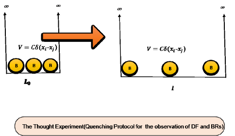
2.1.1 Quench Protocol for the numerical realization of ’Dynamical Fermionization’ and ’Bethe Rapidities’
First we prepare the gas consisting of N atoms(positive scattering length), with a repulsive delta potential of strength
in the ground state. This 1D Bose gas is initially trapped in an infinitely deep box of length . At , the Hamiltonian can be described by
| (3) |
| (7) |
where the infinite walls are defined by the following boundary conditions: Then the above Hamiltonian is quenched by changing the box length from to and the gas is allowed to expand freely in the box of length .
2.2 Path integral formalism for calculating the density of delta interacting 1D Bose by Generalized Feynman-Kac method.
In this section we derive the formula for calculating many body density function used to describe the ’Bethe Rapidities’. We calculate the density in terms of the path integral solutions to the manybody quantum systems with moderate to strong repulsive interactions. Our key derivations will be given at the end of the section by the equations[24-29]. Since these derivations are based on the path integral solutions, in the next two subsections we review our previous work[9-11] on the Quantum Monte Carlo method based on path integration(FK) to solve the eigenvalue problem related to many body Schrödinger equation. Metropolis and Ulam[22] were the first to exploit the relationship between the Schrödinger equation for imaginary time and the random-walk solution of diffusion equation.
2.2.1 Feynman-Kac path Integral representation
Let us consider the initial value problem
| (8) |
where . Applying Trotter[23] product the solution of the above equation can be written as
| (9) |
The integration is done on and Now Eq(6) can be written as
| (10) |
provided converges to and converges to S.
Note that now the integration in . Unfortunately, one cannot justify the existence of S and because of the following reasons:
(a) most paths are not differetiable as a function of time.
(b) does not exist as .
To overcome the difficulty associated with the non-existence of complex valued one replaces t by -it and obtains
| (11) |
where . The solution of the above equation in Feynman representation[24-31] can be given by
| (12) |
where unlike the previously considered complex case
| (13) |
with , is a real valued measure which has a limit as . Namely can be identified with a probability measure, i.e., Wiener measure[32]. In terms of the propagator the solution of eq(9) can be written as[17] where is the time dependent propagator. The solution provided in equation(9) can be written in Feynman-Kac representation as
| (14) |
where is the expectation value of the random variable provided for , the Kato class of potential[33]. A direct benefit of having the above representation is to recover the lowest energy eigenvalue of the Hamiltonian for a given symmetry by applying the large deviation principle of Donsker and Varadhan as follows[34]:
2.2.2 Generalized Feynman-Kac path integration
In dimensions higher than 2, the trajectory X(t) escapes to infinity with probability 1[46] and the important regions of potential are sampled less and less frequently. As a result, Eq(11) converges rather slowly when using original FK formula due to the fact that the underlying diffusion process (i.e., Brownian motion) is nonrecurrent. To speed up the calculation one applies instead the so-called GFK formula. In this section we describe the GFK formula and the measure associated with the underlying stochastic process.
Before we proceed it must be emphasized, as explained earlier in section 2.2.1 that one can associate a stochastic process(e.g., Brownian motion) with the Schrödinger equation by putting the Wiener measure on the space of continuous functions. These continuous functions on [0,T] with values in serve as individual random Brownian motion trajectories called paths, and give rise to path integrals found in FK representation. There is however, yet another way of associating a stochastic process to the Schrödinger equation which leads to a diffusion process other than Brownian motion. Namely, diffusions with stochastic drift term which, unlike Brownian motion, have a stationary distribution.
To this end we consider first the FK solution :
| (15) |
| (16) |
where X(t) is a standard Brownian motion with and = Wiener measure=. The reason behind introducing a new notation is to make a direct association of the infinitesimal generator of the process( where ) for Brownian motion) with the probability on the space , called a diffusion measure . The class of potentials for which the above equation holds is known as Kato class. One can also generalize the representation by allowing a large class of diffusions that, unlike Brownian motion, have stationary distributions. Specifically, for any twice differentiable positive function , one defines a new potential U which is a perturbation of the potential V as follows:
| (17) |
Then one has
which has as a solution:
| (20) |
where the new diffusion has an infinitesimal generator , with adjoint . Here is a stationary density of , or equivalently, . To see the connection between and , observe that for and ,
| (21) |
Moreover, the eigenvalue problem for the stationary equation
| (22) |
and
| (23) |
are related as follows:
| (24) |
| (25) |
To formulate the generalized Feynman-Kac method we first rewrite the Hamiltonian as , where and . We choose the non-negative trial function to be a trial function associated with the symmetry of the problem i.e., and is the trial energy of this reference function. Then Eq(17) can be written in terms of the reference potential as follows:
| (26) |
The diffusion solves the following stochastic differential equation:
.
is summed over all the time steps and is summed over all the trajectories.
The presence of both drift and diffusion terms in the above expression enables the trajectory to be highly localized. As a result, the important regions of the potential are frequently sampled and Eq(11) converges rapidly.
The normalized version of the many body density in the coordinate represetation can be represented as
where
For , only the ground state contributes or in other words,
| (27) |
and
| (28) |
Then the many body density becomes
| (29) | |||||
In the diagonal represetation density function becomes[25]
.
In terms of Feynman-Kac solution the density becomes
| (30) |
The normalized version of many body density can be provided as:
| (31) |
where is the nomalization constant. This is just the density matrix for the lowest energy state for . For propagation time ’t’ the density matrix will be defined in terms of time dependent solution as follows:
| (32) |
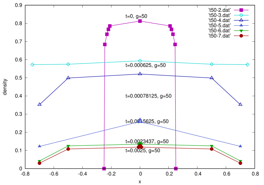
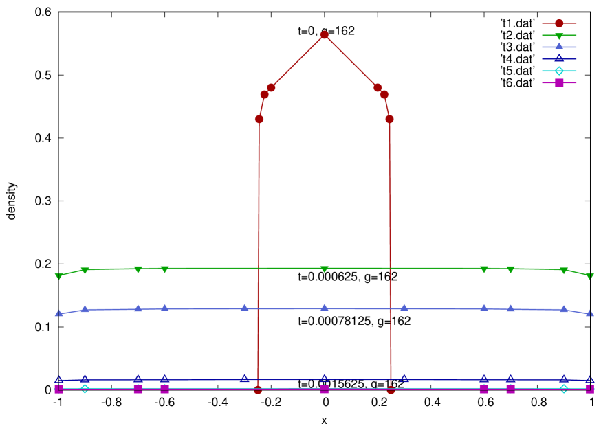
where . Note that which we plot in Fig 2, 3 and 4.
2.3 Correspondence between the asymptotic spatial density(our approach) and Bethe Rapidities of LL system
In Lieb-Liniger model the Schrödinger equation for a Bose gas with N particles in one dimension interacting with repulsive function potential reads as
Now for , the above equation takes the following form:
Also for repulsive interaction we have and .
The bosons as described above behave like fermions in the TG limit and this phenomenon is known as
Fermionization. In this limit the strongly interacting bosons and free fermions share the same energy spectrum but their wave functions
are related as [4].
In ref[18] the expression the time-dependent solution for freely expanding LL gas
which was initially localized by a trapping potential(box or harmonic) was represented as follows :
| (33) |
Here are the position coordinate, are the momentum coordinates and . Also t is the propagation time and subscript B stands for Bosons and c signifies the interaction strength. signify the propagator. The asymptotic wave functions takes the following form:
| (34) | |||
Now the above can be expressed in spatial coordinates by substituting :
| (35) | |||
In Ref[19] the single particle density matrix was defined as:
| (36) |
The correponding momentum distribution is defined as
| (37) |
In Ref[19] it was also shown that the aymptotic form of momentum distrubution of a freely expanding LL gas can be expressed as:
| (38) |
The corresponding spatial density can take the form
| (39) |
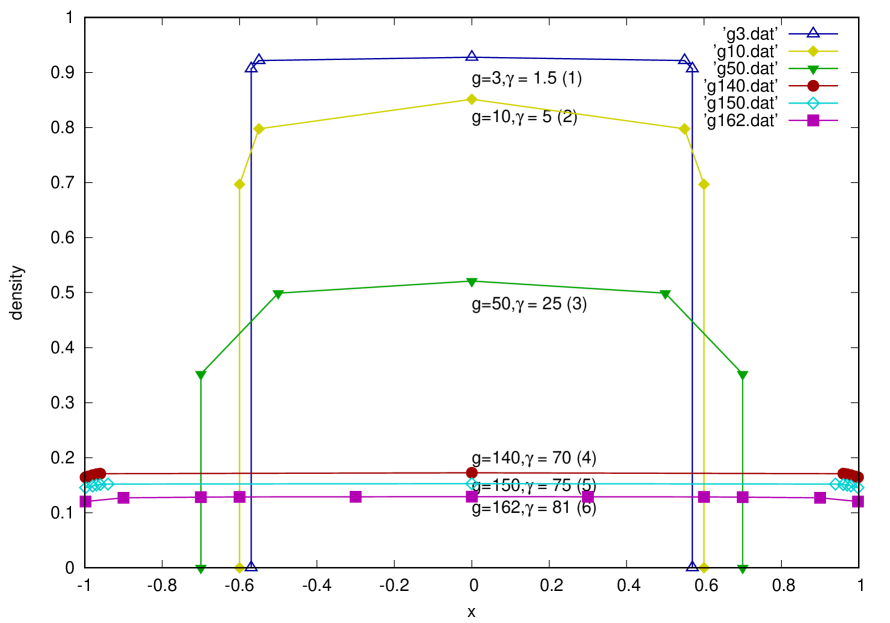
So in Ref[18,19] authors established that the aymptotic single-particle spatial density and momentum density share the same shape in the long time limit. In our case we calculate the many body spatial density as given by Eq(28) and Eq(29). Based on the single-particle proof in their case, we numerically extend the equivalence in shape for the many body density and momentum in the following way. In the LL model a dimensionless parameter was defined as . In our model and (see Eq(2); In LL model the chosen units were . Taking the particle density , can be related to as . Now in Fig 4, we show the the rapidity curve actually resemble the spatial density curves shown in Fig 2 and 3. To do that we fix two asymptotic spatial density curves in Fig 4 for time and for the interaction strengh and and interpolate and extrapolate curves corresponding to interaction strengths , and ad . These curves correpond to the curves in Fig 2 of Ref[6]. Fig 2 of Ref[6] represents vs plots where is the momentum and is the dimensionless parameter as defined before while Fig 4 is actually a plot for vs and is the spatial many body density defined in Eq(28). The equivalence between and has been justified through Eq(34) and Eq(35) as derived in Ref[18,19]. Now since we can integrate the spatial density curves corresponding to interaction strength used in vs plot in the original work of Lieb and Liniger[6] and many body spatial densities calculated from our path integral approach on the same graph and see the similar kind of variation we numerically establish the shape equivalence of aymptotic spatial density and momentum density even in the case of many body case. This justifies our effort to generate ’Bethe Rapidities’ just from the spatial density plot in the long time and infinite interaction limit. The further explanation in favor of a numerical realization of Bethe rapidities through spatial density plots will be provided in section 3(the result section).
2.4 Numerical details for the drifted random walk
For guiding the random walk inside the box of length we use a trial function of the form:
| (40) | |||||
Using the drifted random walk and diffusion(Brownian random walk) inside a box of length , we get the numerical solution for the ground state. The above trial function is used to generate the the drifted random walk. The diffusion part is generated as follows:
2.5 Numerical approximation of the Wiener integrals.
The rigorous justification for the generalization of the formalism discuused in Section 2.2 to dimensions was given by Korzeniwski[48]. Also generalization of the formalism in Section 2.2 to the class of potential for which Feynman-Kac path integral method is valid has been given by Simon[49]. Simon has shown that the Feynman-Kac path integral method is valid for any potential that is an element of Kato Space. Now for , the path integral solution of the Schrödinger equation with potentials that belong to Kato class can be represented in the Wiener measure as:
| (41) |
The above integral can be written as
| (42) |
where is the expected value of the Wiener integral with x the initial position of a random walk .
We can approximate the continuous time integral as a discrete sum as follows:
where is the discrete positions in space determined by the ith step of a random with
and
is a set of independent identically distributed random variables,each having a mean of zero and standard deviation of one. Now is defined as a trial path and is given by
| (43) |
One such trial path is walked if we take discrete steps and evaluate Eq(32) for the set of resulting positions .
The path is viewed as a continuous piecewise linear function starting at x and obtained by joining line segments from the positions .
Let be the results evaluated from Eq(32) for the jth trial path. For N trial paths define the average over all paths as
. Eq(30) can be approximated by
| (44) |
2.6 Parameters used for the work
For the best selection of the parameters, one needs to check the following criteria.
(i) The interactions should be truely two body in nature.
(ii) One needs to know the propagation time to determine whether one can expect to see Bethe rapidities. The expansion velocity time the
time must exceed the initial cloud size. Estimates for the expansion velocity depend on the regime we are at.
(iii) We must make sure that our choices for the coupling constants reflects the three principal regimes.
ideal gas vs mean-field vs Tonks-Girardeau.
For a box in these three regimes our parameters are bounded by the following conditions respectively:
where is the length of the box, is the total number of the particles in the box and is the mass of the particles. We choose in our units.
When we use Gaussian or any hill of height and width we have to make sure that the negative of that is shallow enough to support only one bound state:.
Also, we must make sure that the one particle de-Broglie wavelenghts involved are longer than that of : as Girardeau end was used
to estimate the de-Broglie wavelength.
Number of partcles N=100
Initial Length of the box
Final Length of the box
,
3 Results and Discussions
Employing Eq(11) and Eq(28), we calculate the initial density. For calculating the asymptotic solution we first calculate different time propagated solution taking the ground state solution to be the solution at . Then to calculate the asymptotic solution we use Eq(1). In Fig 2 and Fig 3, we show the plots for different initial and asymptotic densities for the interaction strength and respectively. Comparing Fig 2 and Fig 3, we see that dynamical fermionization is more pronounced with increase with the interaction strength. Both in Fig 2 and 3 the curves with the highest peaks represent the initial density of the strongly interacting Bose gas(t=0). In fig 2 and 3 the flattened curves represent the long time propagation of the intial state. Fig 4 shows the extrapolation and interpolation of spatial curves correspoding to the interaction strength used in fig 2 of Ref[6]. Now curve (1), curve (2) and curve (3) in Fig 4 of this work correspond to the curve (4), curve (5) and curve (6) of Fig 2 of Ref[6] respectively. Also curve (4),curve (5) and curve (6) of this work represent the cases of Fig 2 of Ref[6]. Based on the proofs in Ref[18,19] it can be argued that for sufficiently large times, the momentum distribution coincides with the shape of the space density, even for the many body cases and the flattened asymptotic curves can be accepted as the ’Bethe Rapidities’ as shown in the Fig 2 of Ref[6] and Ref[39].
4 Conclusions and Outlook
Our investigation demonstrates the experimental probing of 1D Bose gases across a spectrum of interaction strengths, from weak to strong, utilizing the ab initio quantum Monte Carlo method. Through a simple yet insightful thought experiment, we have numerically explored Dynamical Fermionization (DF) and Bethe Rapidities (BR) in 1D Bose gases. Our results reveal a remarkable mapping of a Lieb-Liniger (LL) gas with infinite interaction to a non-interacting Fermi gas during its extended evolution post-release from a box-trap. Our numerical findings support some of the previous work in Ref[18,19] for the equivalence between the long time limit of asymptotic spatial and momentum density. As a matter of fact this is the first ever numerical work to show the aforesaid equivalence for the many body density functions also. Despite the absence of thermalization due to integrability, the observation of its relaxation proves captivating, particularly in the context of the abundance of rapidities representing infinite conserved quantities.
To our knowledge, there is a dearth of quantum ab initio treatments for modeling DF and BR in this manner. We emphasize the significance of our approach, where the sole observation of initial space density unfolds the presence of DF and BRs, underscoring the richness and intriguing facets of out-of-equilibrium dynamics. This underscores the importance of space-momentum observation in uncovering novel physics.
Our current endeavor stands as a valuable contribution, offering insights that can inform further investigations into dynamical fermionization in strongly interacting Bose-Fermi mixtures and spinor gases. We anticipate two potential follow-up directions: firstly, an ab initio study of strongly interacting integrable models in the context of 1D Bose-Fermi mixtures, and secondly, a more in-depth exploration of the long-time behavior of 1D spinor gases, acknowledging the potential numerical challenges associated with the latter.
The LL-Bose gas demonstrates a rich interplay between spatial density and momentum distribution as the system transitions from weak to strong interactions. The asymptotic behavior in each regime reflects the unique quantum corelations and phenomena associated with the corresponding interaction strengths, providing a fascinating bridge between the weakly and strongly interacting bosons in one dimension.
Acknowledgements: One of the authors(SD) would like to thank Alliance University for providing support for carrying out the research work
Declaration of interests: The authors have no conflicts of interest to declare. Both the authors have seen and agreed with the contents
of the manuscript and there is no financial interest to report.
Data availability statement: No associated data are available to protect the study participant privacy.
References
- [1] H. A. Bethe, Z Phys,71,205,(1931), https://doi.org/10.1007/bf01341708
- [2] M. Gaudin, Phys. Rev A, 4, 386(1971). DOI:10.1103/PhysRevA.4.386
- [3] J. M. Wilson, M. Malvania, Y. Le, Y. Zhang, M. Rigol, D. S. Weiss,n. Science, 367, 1461(2020). DOI: 10.1126/science.aaz0242
- [4] M. Girardeau, J. Math. Phys. 1, 516(1960) DOI: 10.1063/1.1703687(1960)
- [5] M. Rigol, A. Muramatsu, Phys. Rev. Lett., 94, 240403(2005). DOI: 10.1103/PhysRevLett.94.240403
- [6] E. H. Lieb, W.Liniger, Phys. Rev. 1963, 130, 1605(1963). DOI: 10.1103/PhysRev.130.1605
- [7] I.Bouchoule, B. Doyon, and J. Dubail, SciPost Phys. 9, 044(2020). DOI: 10.21468/scipostphys.9.4.044
- [8] S. S. Alam, T. Skaras, L. Yang, H. Pu, Phys. Rev. Lett., 127, 023002(2021). DOI: 10.1103/PhysRevLett.127.023002
- [9] P. Claverie, M. Cafferel, J. Chem Phys. 88 , 1088 (1988);88, 1100 (1988).DOI: 10.1063/1.454227
- [10] A. Korzeniowski, J. Comp and App Math, 66, 333(1996), doi.org/10.1016/0377-0427(95)00170-0
- [11] S. Datta, Int. J. of Mod Phys.B, 37, 2350024(2023). DOI: 10.1142/S0217979223500248
- [12] M. T. Bachelor, X. W. Guan, N. Oelkers, C. Lee, J. Phys. A, 38, 7787(2005). DOI: 10.1088/0305-4470/38/36/001
- [13] M. Rigol, V. Dunjko, V. Yurovsky, M. Olshanii, Phys. Rev. Lett., 98, 050405(2007). DOI: 10.1103/PhysRevLett.98.050405
- [14] V. Dunjko, V. Lorent, and M. Olshanii, Phys. Rev. Lett. , 86, 5413(2001). DOI: 10.1103/physrevlett.86.5413
- [15] I. Bouchoule, J. Dubail, J. Stat. Mech., 2, 14003(2022). DOI: 10.1088/1742-5468/ac3659
- [16] N. Malvania, Y. Zhang, Y. Le, J. Dubail, M. Rigol, D. S. Weiss, 373, 1129(2021). DOI: 10.1126/science.abf0147
- [17] M. Kac in Proceedings of the Second Berkley Symposium (Berkley Press, California, 1951)
- [18] D.Juki, R. Pezer, T. Gasenzer and H. Buljan, Phys. Rev. A, 78,053602(2008)
- [19] D.Juki, B. Klajn, H. Buljan, Phys. Rev. A, 79, 033612(2009). DOI: 10.1103/PhysRevA.79.033612
- [20] Z. Mei, Z., L.Vidmar, F. Heidrich-Meisner, C. J. Bolech, Phys. Rev. A, 93, 021607(2016).
- [21] M. Olshanii, Phys. Rev.Lett. , 81, 938(1998). DOI: 10.1103/PhysRevLett.81.938
- [22] N. Metropolis and S.J. Ulam, Am. Stat. Assoc.,44, 335(1949),doi:10.1080/01621459.1949.10483310
- [23] H. F. Trotter,Proc. Am. Math. Soc., 1959, 10, 545(1959), doi:10.1090/s0002-9939-1959-0108732-6
- [24] M. D. Donsker, M. Kac, J. Res. Natl. Bur. Stand., 44, 581(1950). DOI: 10.6028/jres.044.050
- [25] R. P. Feynman, Statistical Physics:a set of lectures (Reading Mass.: Addison-Wesley, 1998)
- [26] R. P. Feynman, A. R. Hibbs, Quantum Mechanics and Path Integrals. DOI: 10.1063/1.3048320
- [27] H. S. Schulman, Techniques and Applications of Path Integration. DOI: 10.1063/1.2914703
- [28] A. Korzeniowski, J. L. Fry, D.E. Orr, N. G. Fazleev, Phys. Rev. Lett., 69, 893(1992). DOI: 10.1103/PhysRevLett.69.893
- [29] A. Korzeniowski, J. Comp. App. Math.,66,333(1996) DOI: 10.1016/0377-0427(95)00170-0
- [30] S. Datta, J. L. Fry, N. G. Fazleev, S. A. Alexander, R. L., Coldwell, Phys. Rev. A , 61, 030502(2000). DOI: 10.1103/PhysRevA.61.030502
- [31] S. Datta, V. Dunjko, V., M. Olshanii, 4, 2(2000). DOI: 10.3390/physics401000
- [32] N. Wiener, J. Math and Phys., 131(1923) doi.org/10.1002/sapm192321131
- [33] T. Kato, Commun. Pur. and App. Math., 10, 151(1957). DOI: 10.1002/cpa.3160100201
- [34] M. D. Donsker, S. R. S. and Varadhan, ”Proc Intl. Conf. Func. Sp. Int.” 1975, 15-33. DOI: 10.1073/pnas.72.3.780
- [35] P. Billingsley, Convergence of Probability Measures; (Wiley,New York, NY, USA, 1968.)
- [36] B. Simon, Functional Integrals and Quantum Mechanics (Academic Press, NY), 1979,doi:10.1016/S0079-8169(08)60979-4
- [37] C. A. Tracy, H. Widom, 41, 485204(2008). DOI: 10.1088/1751-8113/41/48/485204
- [38] J. C. Zill, T. D. Wright, K. V. Kheruntsyan, T. Gasenzer, M. J. Davis, N. J. Phys.,18, 045010(2016). DOI: 10.1088/1367-2630/18/4/045010
- [39] G. Lang, F. Hekking, A. Minguzzi, SciPost Phys., 3, 003(2017). DOI: 10.21468/SciPostPhys.3.1.003 doi.org/10.1002/sapm192321131
- [40] F. Ares, S. Scopa and S. J. Wald, Phys. A, 55, 375301(2022)
- [41] A. S. Campbell, D. M. Gangardt, K. V. Kheruntsyan, Phys. Rev. Lett., 114, 125302(2015). DOI: 10.1103/physrevlett.114.125302
- [42] A. Minguzzi, and D. M. Gangardt, Phys. Rev. Lett., 94, 240403(2005). DOI: 10.1103/physrevlett.94.240404
- [43] B. Sutherland, Phys. Rev. Lett., 80, 3678(1998). DOI: 10.1103/physrevlett.80.3678
- [44] W. Tschischik, M. Haque, Preprint at arXiv:1411.554v.
- [45] Y. Zhang, L. Vidmar and M. Rigol, Phys. Rev. A , 99, 063605(2019). DOI: 10.1103/physreva.104.l031303
- [46] I. Karatzas, I and S. E. Shreve, (Springer-Verleg,NY, 1991)
- [47] L. Dubois, G. Thmze, F.,Nogrette, J. Dubail and I. Bouchole, arXiv:2312.15344 v1 [cond-mat.quant-gas] 23 Dec 2023
- [48] A. Korzeneniwski, Stat. and Prob. Lett.,8, 229(1989).
- [49] B. Simon, Schrödinger Semigroups, Bull. Am. Math. Soc.,7,447(1982)
- [50] M. Panfil, F. T. Sant’Ana, J. Stat. Mech. Theory and Experiment, 073103, 2021
- [51] Y. Bezzaz, L. Dubois and I. Bouchoule, SciPost Phys Core 6, 064(2023)