Quality-Aware Image-Text Alignment
for Real-World Image Quality Assessment

Abstract

No-Reference Image Quality Assessment (NR-IQA) focuses on designing methods to measure image quality in alignment with human perception when a high-quality reference image is unavailable. The reliance on annotated Mean Opinion Scores (MOS) in the majority of state-of-the-art NR-IQA approaches limits their scalability and broader applicability to real-world scenarios. To overcome this limitation, we propose QualiCLIP (Quality-aware CLIP), a CLIP-based self-supervised opinion-unaware method that does not require labeled MOS. In particular, we introduce a quality-aware image-text alignment strategy to make CLIP generate representations that correlate with the inherent quality of the images. Starting from pristine images, we synthetically degrade them with increasing levels of intensity. Then, we train CLIP to rank these degraded images based on their similarity to quality-related antonym text prompts, while guaranteeing consistent representations for images with comparable quality. Our method achieves state-of-the-art performance on several datasets with authentic distortions. Moreover, despite not requiring MOS, QualiCLIP outperforms supervised methods when their training dataset differs from the testing one, thus proving to be more suitable for real-world scenarios. Furthermore, our approach demonstrates greater robustness and improved explainability than competing methods. The code and the model are publicly available at https://github.com/miccunifi/QualiCLIP.

1 Introduction

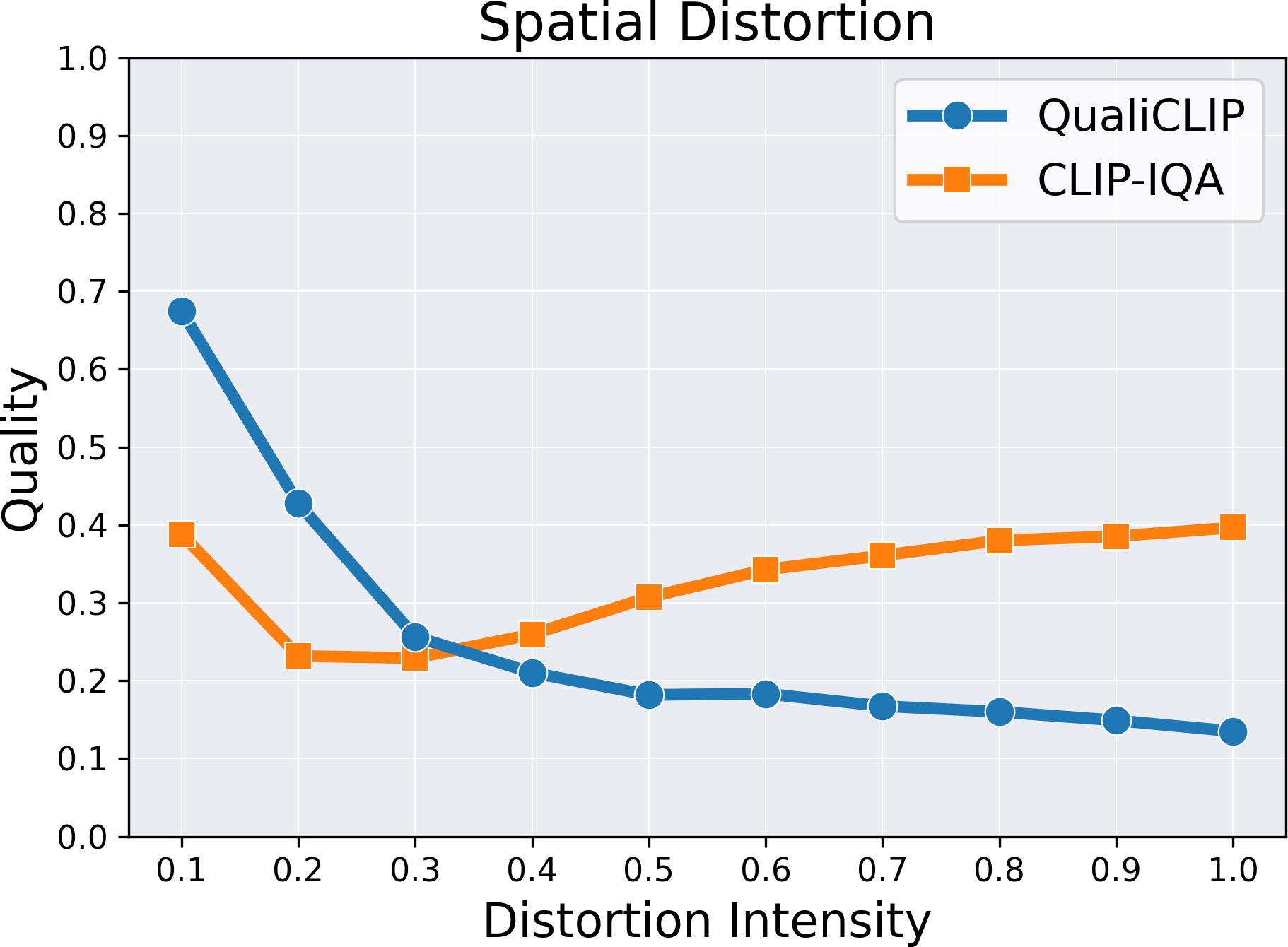
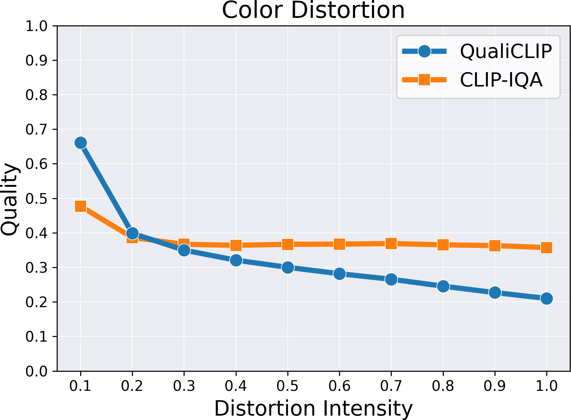
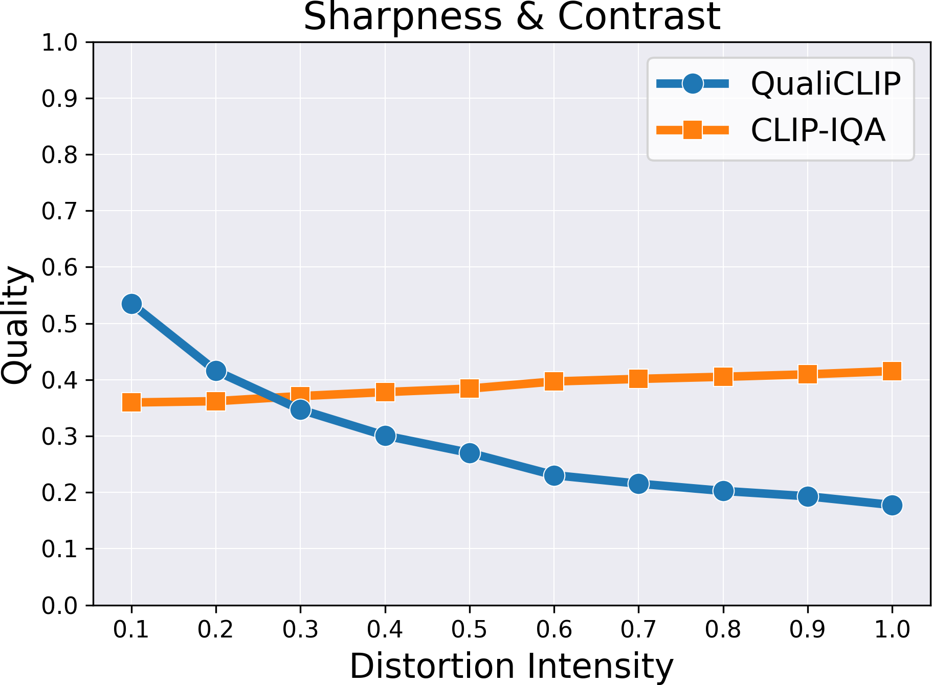
Figure 1: Comparison between the image quality scores predicted by CLIP-IQA [36] and QualiCLIP for increasing distortion intensities of different types of synthetic degradation. We average the results of 1000 randomly sampled images from the KonIQ [10] dataset. Compared to CLIP-IQA, our method corresponds to a higher correlation between the predicted quality scores and the severity of the degradation. The distortion intensities are scaled between 0 and 1 for clearer visualization.

Image Quality Assessment (IQA) aims to automatically evaluate the quality of images in accordance with human judgments, represented by Mean Opinion Scores (MOS). Specifically, No-Reference IQA (NR-IQA) focuses on developing methods that do not require a high-quality reference image and that are consequently more easily applicable in real-world scenarios. NR-IQA plays a critical role in diverse industries and research domains. For example, given the large number of photos that are captured and shared daily on social media platforms, it is imperative to design approaches that can measure image quality objectively to be able to store and process these images effectively. However, for such approaches to be reliable, they need to exhibit strong generalization capabilities.

Most NR-IQA methods are opinion-aware, i.e. they require labeled mean opinion scores as supervision during the training process [33, 7, 41, 23, 1, 28]. Some approaches, such as HyperIQA [33] or TReS [7], directly train the model parameters on IQA datasets. Other methods, namely CONTRIQUE [23] or ARNIQA [1], train first an image encoder on unlabeled data via self-supervised learning and then a linear regressor using the MOS. However, annotating IQA datasets is very expensive and resource-intensive, as several human ratings are needed for each image for the MOS to be reliable. For example, the FLIVE dataset [39], which contains 40K real-world images, required about 4M ratings, up to 50 for a single image. The requirement for human annotations significantly hinders the scalability of opinion-aware approaches. In addition, these methods show limited generalization capabilities and thus applicability to real-world scenarios, as their performance significantly deteriorates in cross-dataset settings, i.e. when considering testing datasets different from the training one. To remove the requirement for labeled MOS, several opinion-unaware methods have been proposed [20, 4, 8]. For instance, CL-MI [4] introduces a two-stage self-supervised approach that employs two different training strategies for synthetically and authentically degraded images. However, existing opinion-unaware methods obtain considerably worse performance than supervised approaches in cross-dataset experiments, thus demonstrating limited applicability.

In this context, we propose to take advantage of recent advancements in vision-language models by presenting a self-supervised opinion-unaware approach based on CLIP [26]. Recently, CLIP-based methods achieved promising performance in the NR-IQA task [36, 42, 32]. For example, CLIP-IQA [36] proposes to compute the quality score by measuring the similarity between the image and the two quality-related antonym prompts without any task-specific training. However, CLIP struggles to generate quality-aware image representations [42, 13], as it focuses more on the high-level semantic information rather than on the low-level characteristics of the images. To support this claim, we randomly sample 1000 images from the KonIQ [10] dataset and synthetically degrade them with several distortions using increasing levels of intensity. Then, we compute the quality score of each image through CLIP-IQA and average the results. We expect the more degraded versions of the images to correspond to lower quality scores. However, Figure 1 shows that CLIP-IQA demonstrates a low correlation between the predicted quality and the degree of the distortion. Therefore, CLIP proves not to be intrinsically quality-aware.

To address this issue, we propose a quality-aware image-text alignment strategy to fine-tune the CLIP image encoder so that it generates representations that correlate with the inherent quality of the images. We start by synthetically degrading pairs of pristine images using increasing levels of intensity. Then, we measure the similarity between each image and antonym prompts referring to image quality, such as “Good photo” and “Bad photo”. Finally, we employ a training strategy based on a margin ranking loss [13, 16, 7] that allows us to achieve two objectives. First, we want CLIP to generate similar representations for images of comparable quality, i.e. exhibiting the same amount of distortion. Second, the similarity between each of the antonym prompts and the increasingly degraded versions of the images must correlate – in opposite directions – with the intensity of the distortion. Our approach, named QualiCLIP (Quality-aware CLIP), is both self-supervised and opinion-unaware, as we do not rely on any form of supervision – especially MOS – at any step of the training process. Thanks to our training strategy, the image-text alignment in the CLIP embedding space focuses on the low-level image characteristics rather than the semantics. Consequently, QualiCLIP generates quality-aware representations that correlate with the amount of degradation exhibited from the images, as shown in Fig. 1. The experiments show that the proposed approach obtains significant performance improvements – up to a 20% gain – over other state-of-the-art opinion-unaware methods on several datasets with authentic distortions. In addition, QualiCLIP outperforms supervised techniques in the cross-dataset setting, exhibiting more suitability for real-world applications. Moreover, the gMAD [21] competition and visualization with gradCAM [29] show that QualiCLIP demonstrates both greater robustness and enhanced explainability than competing methods. We summarize our contributions as follows:

• We propose QualiCLIP, a CLIP-based self-supervised opinion-unaware approach for NR-IQA that does not require any supervision, especially MOS;

• We introduce a quality-aware image-text alignment strategy based on ranking increasingly degraded pairs of images according to their similarity to quality-related antonym prompts. After training, CLIP generates image representations that correlate with their intrinsic quality;

• Our method obtains significantly better results than other opinion-unaware approaches and even outperforms supervised techniques in cross-dataset experiments, proving to be more suitable for real-world scenarios. Moreover, QualiCLIP exhibits greater robustness and improved explainability than competing methods.

2 Related Work

No-Reference Image Quality Assessment Due to its wide range of applications in real-world scenarios, in recent years research on NR-IQA has gained significant momentum [33, 7, 23, 1, 4]. Several methods achieved promising performance by relying on supervised learning [33, 7, 23, 1]. Some approaches directly employ the labeled MOS during model training [33, 23, 41]. For example, HyperIQA [33] proposes a self-adaptive hypernetwork that separates content understanding from quality prediction. Another research direction involves a self-supervised pre-training of an encoder on unlabeled images, followed by the training of a linear regressor using the annotated MOS [23, 28, 1]. For instance, ARNIQA [1] pre-trains the encoder by maximizing the similarity between different images degraded in the same way. Supervised methods require expensive labeled MOS, either for training the encoder or the regressor. This requirement is removed by opinion-unaware approaches [24, 40, 20, 4, 31]. Some of them, such as NIQE [24], are based on natural scene statistics [24, 40], while others employ self-supervised learning [20, 4, 31, 8]. For example, CL-MI [4] pre-trains an encoder on synthetic data and then fine-tunes it on authentic images via a mutual information-based loss. In this work, we propose a self-supervised opinion-unaware approach that relies solely on CLIP and achieves state-of-the-art results on several datasets with authentic distortions.

CLIP for NR-IQA CLIP has achieved impressive performance in several low-level vision tasks, such as image and video restoration [13, 18, 2] and quality assessment [36, 42, 32, 38, 37]. CLIP-IQA [36] is the first work that studied the capabilities of CLIP in assessing the quality and abstract perception of images without task-specific training. In addition, the authors train a model named CLIP-IQA+ based on learning two antonym prompts using labeled MOS. On the contrary, LIQE [42] proposes a multi-task learning approach that fine-tunes CLIP on multiple IQA datasets at once in a supervised way. The most similar to our work is the concurrent GRepQ [32], a self-supervised method based on a low-level encoder and a high-level CLIP-based one. CLIP is fine-tuned by separating higher and lower-quality groups of images within the same batch with a contrastive loss depending on their predicted quality, obtained by measuring their similarity to antonym text prompts. GRepQ predicts the final quality score by combining the features of the two encoders and feeding them as input to a linear regressor, which is trained on IQA datasets using the labeled MOS. In contrast, we present a CLIP-only self-supervised approach that removes the need for a low-level encoder. We propose to synthetically degrade pairs of images with increasing levels of intensity and make our model learn to rank them through a ranking loss according to their degree of distortion. The ranking is based directly on the similarity between the text features and each of the antonym prompts, instead of relying on the predicted quality as in GRepQ. Also, differently from GRepQ, we do not require any form of supervision at any step of our approach.

Learning to Rank Learning to rank images has proven to be an effective technique for image quality and aesthetics assessment [16, 7, 11, 35, 20, 27]. RankIQA [16] proposes to pre-train a Siamese network in an unsupervised way by directly ranking the quality of increasingly degraded images. Then, the model is fine-tuned on IQA datasets with an MSE loss using the ground-truth MOS. VILA [11] tackles image aesthetics assessment by fine-tuning CLIP using image-comment pairs. Then, the authors train a residual projection by learning to rank the quality – expressed as the similarity between the image and a single prompt – of a single pair of images, according to their labeled MOS. In contrast, we design an approach that does not require any form of supervision during training. Indeed, we fine-tune the CLIP image encoder by learning to rank the similarity between two antonym prompts and multiple increasingly degraded pairs of images, according to the severity of their distortion. At the same time, we force our model to generate consistent representations for images exhibiting the same level of degradation.

3 Proposed Approach

We propose a quality-aware image-text alignment strategy to make CLIP generate representations that correlate with the intrinsic quality of the images. First, we synthetically degrade pairs of crops with increasing levels of intensity. Then, we fine-tune the CLIP image encoder by ranking the similarity between two antonym prompts and the increasingly distorted image pairs, based on their degree of degradation, while guaranteeing consistent representations for images with comparable quality. We keep the CLIP text encoder fixed. We do not employ any supervision – particularly MOS – at any step of the training process.

3.1 CLIP preliminaries

CLIP (Contrastive Language-Image Pre-training (CLIP) [26]) is a vision-language model trained on a large-scale dataset with a contrastive loss to semantically align images and corresponding text captions in a shared embedding space. CLIP comprises an image encoder $\psi_{I}$ and a text encoder $\psi_{T}$. Given an image $I$, the image encoder extracts its feature representation $x=\psi_{I}(I)\in\mathbb{R}^{d}$, where $d$ is the CLIP embedding space dimension. For a given text caption $T$, each tokenized word is mapped to the token embedding space $\mathcal{W}$ through a word embedding layer $E_{w}$. Then, the text encoder $\psi_{T}$ is employed to generate the textual feature representation $y=\psi_{T}(E_{w}(T))\in\mathbb{R}^{d}$ from the token embeddings. Thanks to its training strategy, CLIP generates similar representations within the common embedding space for images and text expressing the same concepts.

3.2 Synthetic Degradation with Increasing Levels of Intensity

To make our approach self-supervised, we propose to synthetically degrade unlabeled pristine images using progressively higher levels of intensity. In this way, we can train our model to rank the different versions of each image according to the severity of their degradation. Following [1], we consider 24 distinct degradation types spanning the 7 distortion groups $\mathcal{G}\!=\!\{\mathcal{G}_{1},\ldots,\mathcal{G}_{7}\}$ defined by the KADID [15] dataset. These groups are: 1) Brightness change; 2) Blur; 3) Spatial distortions; 4) Noise; 5) Color distortions; 6) Compression; 7) Sharpness & contrast. Each distortion has $L\!=\!5$ levels of intensity. Figure 2 shows some examples of degraded images for varying degrees of intensity. See the supplementary material for more details on the specific degradation types. Each distortion group is defined as $\mathcal{G}_{i}\!=\!\{\ldots,F^{ij},\ldots\}$, where $i\!\in\!\{1,\ldots,7\}$ indicates the index of the distortion group within $\mathcal{G}$ and $j\!\in\!\{1,\ldots,\left|G_{i}\right|\}$ refers to the index of the degradation type within $\mathcal{G}_{i}$, with $\left|\cdot\right|$ that represents the cardinality.

Given a training image, we start by extracting a pair of random overlapping crops. Then, we randomly sample $D\!=\!1$ distortion groups and a degradation within each group. We apply the $D$ distortions to both crops using $L\!=\!5$ distinct levels of intensity, resulting in $L$ pairs of equally degraded crops, one for each level. Contrary to [16], we obtain two images for each degree of distortion. When considering two such pairs of crops, we can infer which has a higher quality, based on the corresponding level of degradation. We leverage this information to train our model with a ranking loss.

(a) Color distortion

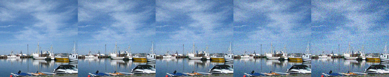
(b) Noise

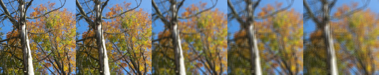
(c) Blur

(d) Spatial distortion

Figure 2: Examples of synthetic degradations for $L\!=\!5$ increasing levels of intensity.

3.3 Quality-Aware Image-Text Alignment

As Fig. 1 shows, CLIP struggles to generate accurate quality-aware image representations that correlate with the severity of the degradation. To address this issue, we propose a quality-aware image-text alignment strategy to fine-tune the CLIP image encoder. The idea of our approach is that given two degraded versions of the same image, a prompt referring to high image quality – such as “Good photo” – should be more similar to the less degraded version. The opposite consideration applies when considering a prompt referring to low image quality, such as “Bad photo”. At the same time, two images with overlapping content and equal degree of degradation should have comparable similarities to such a pair of quality-related prompts, which we refer to as antonym prompts [36]. Note that, given two random images with completely different content, we can not make any assumptions about their relative quality, or, in other words, their similarity to the prompts. Our training strategy leverages multiple pairs of increasingly degraded images to achieve two objectives: O1): we want CLIP to generate consistent representations for images of similar quality, i.e. showing the same amount of distortion; O2): the similarity between each of the antonym prompts and the distinct versions of the images must correlate – in opposite directions – with the corresponding level of degradation.

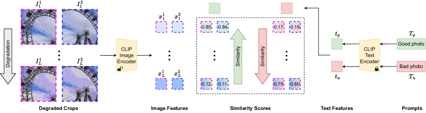
Figure 3: Overview of the proposed quality-aware image-text alignment strategy. Starting from a pair of two random overlapping crops from a pristine image, we synthetically degrade them with $L$ increasing levels of intensity, resulting in $L$ pairs. Then, given two quality-related antonym prompts, we fine-tune the CLIP image encoder by ranking the similarity between the prompts and the images, according to their corresponding level of degradation. At the same time, for each pair of equally distorted crops, we force the similarity between the crops and the prompts to be comparable.

Let $I_{i}^{1}$ and $I_{i}^{2}$ be the $i$-th pair of increasingly degraded crops obtained as detailed in Sec. 3.2, where $i\in\{1,\ldots,L\}$ and $L\!=\!5$ is the number of considered distortion levels. For $i,j\in\{1,\ldots,L\}$ with $j>i$, the $j$-th pair of crops is more degraded than the $i$-th one. Given each pair of crops, we extract the corresponding features through the CLIP image encoder $\psi_{I}$, resulting in $x_{i}^{1}=\psi_{I}(I_{i}^{1})$ and $x_{i}^{2}=\psi_{I}(I_{i}^{2})$. Similarly to [36], we remove the positional embedding to relax the CLIP’s requirement of fixed-size inputs. Let $T_{p}$ and $T_{n}$ be a pair of antonym prompts related to image quality, such as “Good photo” and “Bad photo”. We refer to $T_{p}$ and $T_{n}$ as “positive” and “negative” prompts, respectively. We employ the CLIP text encoder $\psi_{T}$ to extract the text features associated with the prompts, obtaining $t_{p}=\psi_{T}(T_{p})$ and $t_{n}=\psi_{T}(T_{n})$. We normalize both the image and text features to have a unit $L_{2}$-norm.

To achieve objective O1, we propose to employ a consistency loss term to guarantee that the similarity between the features of the prompts and those of each of the two images composing each degraded pair is comparable. We assume that two overlapping crops extracted from the same image have a comparable quality [28, 43]. We rely on a margin ranking loss [13, 16, 7] defined as:

where $c(\cdot)$ stands for the cosine similarity and the margin $m_{cons}$ is a hyperparameter. Intuitively, $m_{cons}$ must be close to 0 to force the similarities between the prompts and each of the two crops to be comparable.

Given the $i$-th level of synthetic degradation, with $i\in\{1,\ldots,L\}$, we assume that the quality of the two distorted crops of the $i$-th pair is higher than that of the two images composing the $(i+1)$-th one [16, 27]. Thus, we enforce that the similarity between the features of the positive prompt and those of two crops is higher than when considering more degraded versions of the two crops. Specifically, we define a margin ranking loss as:

where $c(\cdot)$ represents the cosine similarity and the margin $m_{rank}$ is a hyperparameter. The opposite of the consideration made above applies when we take into account the negative prompt. Therefore, we add a loss term to impose that the similarity between the features of the negative prompt and those of two crops is lower than when considering more degraded versions of the two crops:

with $c(\cdot)$ and $m_{rank}$ defined as above. Intuitively, we need to set $m_{rank}\!>>\!0$ as we aim for a noticeable difference between the similarities of the prompts and the increasingly degraded versions of the two crops. The combination of $\mathcal{L}_{pos}$ and $\mathcal{L}_{neg}$ allows us to achieve objective O2.

The final training loss used to fine-tune the CLIP image encoder is given by:

$$\mathcal{L}=\lambda_{cons}\mathcal{L}_{cons}+\lambda_{pos}\mathcal{L}_{pos}+\lambda_{neg}\mathcal{L}_{neg}$$ (4)

where $\lambda_{cons}$, $\lambda_{pos}$, and $\lambda_{neg}$ represent the loss weights. Figure 3 shows an overview of our training strategy. Given that we do not employ any labeled MOS, our approach is both self-supervised and opinion-unaware. Thanks to the proposed training strategy, CLIP learns an image-text alignment not based on high-level semantics, but rather on low-level image characteristics, such as noise and blur. As a result, QualiCLIP generates representations that correlate with the intrinsic quality of the images, as shown in Fig. 1.

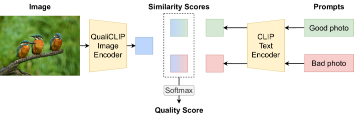
Figure 4: Overview of the final quality score computation strategy. The quality score is given by the softmax of the similarities between the image features and the text features of two antonym prompts.

At inference time, given an image $I$, we extract its features $x$ using the CLIP image encoder. Then, we compute the cosine similarity between $x$ and the features $t_{p}$ and $t_{n}$ of the antonym prompts, resulting in $s_{p}$ and $s_{n}$. Finally, similar to [36], we obtain the final quality score $q\!\in\![0,1]$ by using the softmax:

$$q=\frac{e^{s_{p}}}{e^{s_{p}}+e^{s_{n}}}$$ (5)

Figure 4 provides an overview of the final quality score computation. Note that, since we keep the CLIP text encoder weights frozen, we need to compute the text features of the antonym prompts just once, and we can use them both for training and inference. Therefore, at inference time the computational cost of our method is the same as an image-encoder-only model with the same backbone.

We recall that the authors of GRepQ [32] use a strategy similar to the one shown in Fig. 4 to predict the quality of all the images comprising a training batch. Then, they divide the images into a high-quality and a low-quality group. Finally, they fine-tune the CLIP image encoder with a contrastive loss by maximizing the intra-group similarity and minimizing the inter-group one. In contrast, we consider multiple pairs of increasingly synthetically degraded crops. We rely on $\mathcal{L}_{cons}$ to fine-tune the CLIP image encoder so that it generates consistent representations for images exhibiting the same degree of distortion. At the same time, we use $\mathcal{L}_{pos}$ and $\mathcal{L}_{neg}$ to train our model to rank the similarity between two antonym prompts and the images, according to their level of degradation. Thanks to our training strategy, CLIP yields more accurate quality-aware image representations.

4 Experimental Results

4.1 Datasets

We train our model using the 140K pristine images of the KADIS dataset [15]. Given a training image, we synthetically degrade it by employing the strategy detailed in Sec. 3.2. We validate and test the proposed approach on IQA datasets with synthetic and authentic distortions, respectively. These datasets contain a set of degraded images annotated with human judgments of picture quality in the form of a Mean Opinion Score (MOS). For validation, we consider two synthetically degraded datasets: LIVE [30] and TID2013 [25]. LIVE stems from 29 reference images, each distorted with 5 types of degradation at 5 levels of intensity, resulting in 779 images. Conversely, TID2013 contains 3000 images degraded with 24 distinct distortions at 5 levels of intensity, with 25 reference images as the base. For testing, we consider four datasets with authentic distortions: KonIQ [10], CLIVE [6], FLIVE [39], and SPAQ [5]. KonIQ contains 10K images sampled from the YFCC100M [34] database. CLIVE consists of 1162 images captured with a wide range of mobile devices. FLIVE is the largest existing dataset for NR-IQA and is composed of about 40K real-world images. SPAQ comprises 11K high-resolution photos taken with several smartphones. Following [5], we resize the SPAQ images so that the shorter side is 512.

Table 1: Comparison between QualiCLIP and competing opinion-unaware methods on datasets with authentic distortions. Best and second-best scores are highlighted in bold and underlined, respectively. Relative gains over the best-performing baseline are indicated in green. OU indicates Opinion-Unaware version as explained in Sec. 4.3.

	KonIQ		CLIVE		FLIVE		SPAQ		Average
Method	SRCC	PLCC	SRCC	PLCC	SRCC	PLCC	SRCC	PLCC	SRCC	PLCC
NIQE [24]	0.526	0.534	0.450	0.493	0.158	0.221	0.703	0.712	0.459	0.490
IL-NIQE [40]	0.493	0.519	0.438	0.503	0.165	0.209	0.710	0.717	0.452	0.487
CONTRIQUE-OU [23]	0.637	0.630	0.394	0.422	0.199	0.228	0.676	0.680	0.477	0.490
Re-IQA-OU [28]	0.558	0.550	0.418	0.444	0.218	0.238	0.616	0.618	0.453	0.463
ARNIQA-OU [1]	0.741	0.760	0.484	0.558	0.299	0.362	0.789	0.797	0.578	0.619
CL-MI [4]	0.645	0.645	0.507	0.525	0.257	0.293	0.701	0.702	0.528	0.541
CLIP-IQA [36]	0.699	0.733	0.611	0.593	0.287	0.349	0.733	0.728	0.583	0.601
GRepQ-OU [32]	0.768	0.788	0.740	0.769	0.327	0.438	0.805	0.809	0.660	0.701
QualiCLIP	0.815	0.837	0.753	0.790	0.393	0.496	0.843	0.855	0.701	0.745
	+6.1%	+6.2%	+1.8%	+2.7%	+20.2%	+13.2%	+4.7%	+5.7%	+6.2%	+6.2%

4.2 Implementation Details

We rely on a ResNet50 [9] as the backbone for CLIP. Similar to [36], we remove the positional embedding from the encoder to allow our model to take images of any resolution as input. The dimension $d$ of the CLIP embedding space is 1024. Differently from [32], we do not train a projector head on top of the CLIP image encoder. We keep the CLIP text encoder frozen. Similar to [38, 37], we employ multiple pairs of antonym prompts. We train our model for 3 epochs using an AdamW [17] optimizer with a weight decay and a learning rate of $1e\!-\!2$ and $1e\!-\!9$, respectively. During training, we employ a patch size of 224 and a batch size of 16. We set the margins $m_{cons}$ in Eq. 1 and $m_{rank}$ in Eqs. 2 and 3 to $2.5e\!-\!3$ and $6.75e\!-\!2$, respectively. The loss weights $\lambda_{cons}$, $\lambda_{pos}$ and $\lambda_{neg}$ in Eq. 4 are all equal to 1. At inference time, our model takes the whole image as input and outputs a single quality score.

4.3 Quantitative Results

Evaluation protocol We evaluate the performance using Spearman’s rank order correlation coefficient (SRCC) and Pearson’s linear correlation coefficient (PLCC), which measure prediction monotonicity and accuracy, respectively. Higher values of SRCC and PLCC correspond to better results. Following [3], we pass the quality predictions through a four-parameter logistic non-linearity before computing PLCC.

We compare our approach to state-of-the-art methods in two different settings: zero-shot and cross-dataset. Note that our method remains consistent across both settings; the only variation lies in the baselines we compare against. For a fair comparison, we compute the results of each baseline using our evaluation protocol by employing the official pre-trained model if available or training it from scratch using the original hyperparameters. In the zero-shot setting, we only consider opinion-unaware methods [24, 40, 4, 36] and approaches that, with slight modifications, can function without requiring MOS [23, 28, 1, 32]. In particular, we follow the original paper for GRepQ [32], while for methods based on a linear regressor [23, 28, 1], such as CONTRIQUE [23], we use a NIQE-style framework on the extracted image features, similar to [4]. We evaluate the performance using the full datasets for testing. In the cross-dataset setting, we compare with supervised methods [33, 7, 23, 28, 1, 36, 32] using testing datasets different from the training one, simulating real-world scenarios. Here, we use the full datasets both for training and testing.

Zero-shot setting We report the results for the zero-shot setting in Tab. 1. We observe that the proposed approach achieves state-of-the-art results on all the testing datasets. QualiCLIP obtains significant improvements compared to the other methods, with about a 20% and a 6% gain over the best-performing baseline on the FLIVE dataset and on average, respectively. In particular, the improvement over CLIP-IQA proves that the proposed training strategy makes CLIP generate image representations that better correlate with their intrinsic quality. In addition, we recall that GRepQ employs a low-level encoder and a high-level fine-tuned CLIP-based encoder. Despite relying solely on CLIP, QualiCLIP outperforms GRepQ, further confirming the effectiveness of our quality-aware image-text alignment strategy.

Table 2: Comparison between QualiCLIP and supervised methods trained on FLIVE [39]. We report the performance on several datasets with authentic distortions. Best and second-best scores are highlighted in bold and underlined, respectively. Relative gains (losses) over the best-performing baseline are indicated in green (red).

		KonIQ		CLIVE		SPAQ		Average
Method	Opinion-Unaware	SRCC	PLCC	SRCC	PLCC	SRCC	PLCC	SRCC	PLCC
HyperIQA [33]	✗	0.738	0.742	0.736	0.743	0.653	0.658	0.709	0.714
TReS [7]	✗	0.748	0.751	0.735	0.751	0.743	0.741	0.742	0.748
CONTRIQUE [23]	✗	0.779	0.781	0.734	0.751	0.817	0.825	0.777	0.786
Re-IQA [28]	✗	0.789	0.825	0.719	0.770	0.826	0.830	0.778	0.808
ARNIQA [1]	✗	0.787	0.804	0.734	0.777	0.841	0.849	0.787	0.810
CLIP-IQA+ [36]	✗	0.784	0.801	0.707	0.732	0.751	0.750	0.747	0.761
GRepQ [32]	✗	0.807	0.812	0.768	0.785	0.828	0.836	0.801	0.811
QualiCLIP	✓	0.815	0.837	0.753	0.790	0.843	0.855	0.804	0.827
		+1.0%	+3.1%	-2.0%	+0.6%	+0.2%	+0.7%	+0.3%	+2.0%

Cross-dataset setting Table 2 shows the results for the cross-dataset setting. This experiment allows us to compare the generalization capabilities of our model with supervised methods. We employ FLIVE as the training dataset for the baselines. We do not compare with LIQE [42] as it requires multiple datasets for training. It is important to highlight that this experimental setting is unfavorable to the proposed approach. Indeed, in contrast with the competing methods, we do not use any labeled MOS during the training process. Nevertheless, we observe that QualiCLIP outperforms all the baselines. In particular, our method obtains a significant improvement over ARNIQA, which has shown impressive generalization capabilities [1]. This experiment shows that most of the supervised methods struggle to generalize to datasets different from the training ones. In contrast, despite not requiring MOS, our method consistently achieves impressive performance on all the testing datasets, proving to be more suitable for applications in real-world scenarios. Moreover, by comparing Tab. 1 and Tab. 2, we observe that QualiCLIP is the only opinion-unaware approach that manages to obtain better results than supervised methods.

4.4 Ablation Studies

We conduct ablations studies on the LIVE and TID2013 synthetic datasets to evaluate the individual contribution of each component of our approach.

Table 3: Ablation studies on the loss terms of Eq. 4 (left) and on the training strategy (right). We report the performance on the LIVE and TID2013 synthetic datasets. Best and second-best scores are highlighted in bold and underlined, respectively.

			LIVE		TID2013
$\mathcal{L}_{cons}$	$\mathcal{L}_{pos}$	$\mathcal{L}_{neg}$	SRCC	PLCC	SRCC	PLCC
✓	✗	✗	0.601	0.617	0.504	0.610
✗	✓	✗	0.651	0.627	0.515	0.592
✗	✗	✓	0.871	0.852	0.609	0.657
✓	✓	✗	0.670	0.649	0.523	0.605
✓	✗	✓	0.881	0.859	0.623	0.675
✗	✓	✓	0.861	0.858	0.603	0.636
✓	✓	✓	0.887	0.880	0.626	0.679

	LIVE		TID2013
Ablation	SRCC	PLCC	SRCC	PLCC
D = 2	0.841	0.817	0.618	0.676
L = 3	0.814	0.781	0.587	0.661
quality-based	0.827	0.816	0.552	0.663
w/ pos. emb.	0.879	0.866	0.629	0.674
QualiCLIP	0.887	0.880	0.626	0.679

Loss terms We study the importance of each loss term in Eq. 4 and report the results in Tab. 3 (left). First, we notice that $\mathcal{L}_{cons}$ by itself is insufficient for making CLIP generate quality-aware representations, as it does not exploit the information provided by the intrinsic ranking of the increasingly degraded crops. Nevertheless, $\mathcal{L}_{cons}$ consistently yields a positive impact when combined with any of the other loss terms. Then, we observe that despite being symmetrical to $\mathcal{L}_{pos}$, $\mathcal{L}_{neg}$ seems to be more crucial for the training process. Given that $\mathcal{L}_{neg}$ involves the alignment between the images and the negative prompt, this outcome suggests that such prompt holds more significance in the quality score computation as in Fig. 4. We provide a detailed discussion of this hypothesis in the supplementary material. Nevertheless, Tab. 3 (left) shows that combining the three loss terms achieves the best results, proving that they are all crucial for training CLIP to generate accurate quality-aware image representations.

Training strategy We evaluate the performance achieved by modified versions of our approach: 1) $D\!=\!2$: we apply two sequential degradations to each crop in Sec. 3.2 instead of just one; 2) $L\!=\!3$: we consider only 3 levels of degradation in Secs. 3.2 and 3.3 instead of 5; 3) we directly use the predicted quality scores associated to each degraded crop instead of its similarity to the antonym prompts in the ranking loss computation; 4) w/ pos. emb.: we relax the CLIP’s requirement of fixed-size inputs by interpolating the positional embedding instead of removing it. Table 3 (right) shows the results. First, we note that employing more than one distortion leads to a decrease in performance. This is because the synthetic degradation becomes too severe independently of the level of intensity, making it overly challenging for the model to rank the crops effectively. Moreover, considering only 3 levels of degradation provides less information to the model during training compared to using 5 different levels, and thus corresponds to worse results. Then, we observe that directly employing the predicted quality scores in the ranking loss instead of the similarity to the prompts achieves poor performance. We attribute this outcome to an increased discrepancy between the CLIP training and fine-tuning process. Indeed, while the predicted quality scores originate from two prompts (see Fig. 4), the proposed strategy considers multiple pairs of single images and texts, which we argue is more similar to the technique used for training CLIP [26]. Finally, employing an interpolated positional embedding produces comparable results to its removal. This contrasts with observations in CLIP-IQA, where the authors noted a significant performance decline when the positional embedding was used [36]. We suppose that in our case, the model learns to adjust to the presence or absence of the positional embedding during the fine-tuning process, thus achieving similar outcomes.

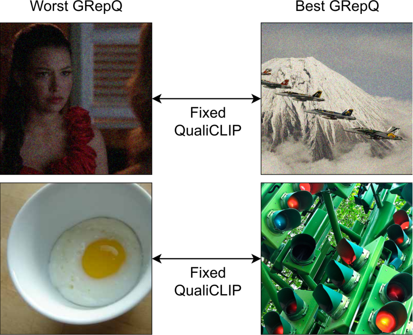
(a)

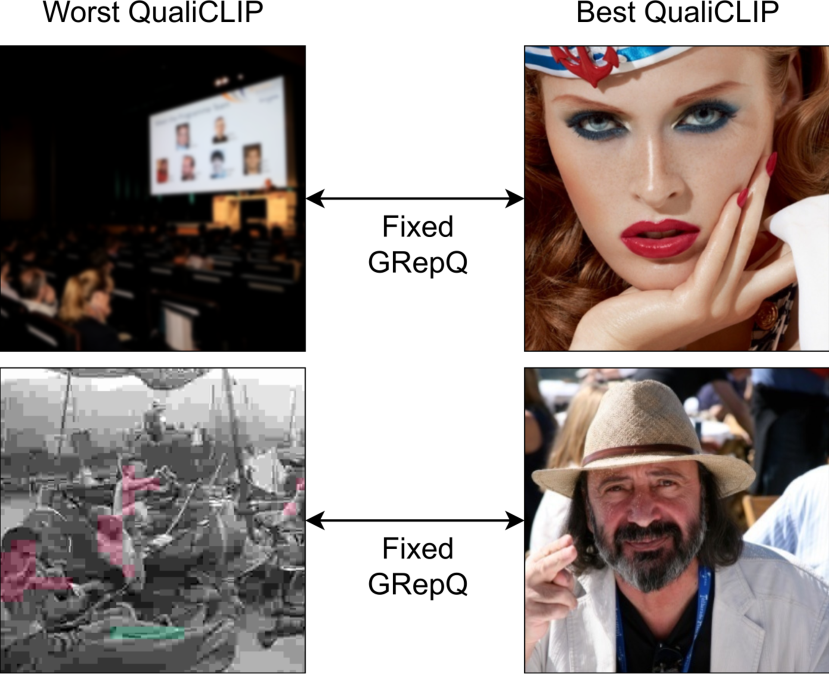
(b)

Figure 5: gMAD [21] competition results between QualiCLIP and GRepQ [32]. (a): Fixed QualiCLIP at a low- (top) and high-quality (bottom) level, respectively. (b): Fixed GRepQ at a low- (top) and high-quality (bottom) level, respectively.

4.5 Additional Experiments

We evaluate the robustness and the explainability of our model through the gMAD [21] competition and a gradCAM [29] visualization, respectively. We report additional experiments in the supplementary material.

gMAD To assess the robustness of our model we carry out the group maximum differentiation (gMAD) competition [21]. In particular, we compare QualiCLIP against GRepQ [32] using the Waterloo Exploration Database [19] dataset, which comprises 95K synthetically degraded images without MOS annotations. In this evaluation, one model is fixed to function as a defender, and its quality predictions are grouped into distinct levels. The other model assumes the role of the attacker, tasked with identifying image pairs within each level that exhibit the greatest quality difference. For a model to demonstrate robustness, the selected image pairs should show comparable quality when acting as the defender while exhibiting a notable quality disparity when assuming the role of the attacker. We observe that when we fix QualiCLIP at a low-quality level (Fig. 5(a) top), GRepQ fails to find picture pairs with an obvious quality difference. When considering a high-quality level (Fig. 5(a) bottom), the image pair identified by GRepQ shows a slight quality gap. However, when assuming the role of the attacker (Fig. 5(b)), QualiCLIP successfully exposes the failures of GRepQ, as it pinpoints image pairs displaying a significant quality disparity. Therefore, our approach demonstrates superior robustness compared to GRepQ.

gradCAM visualization We evaluate the explainability of our model and CLIP-IQA via a gradCAM [29] visualization. gradCAM is a visualization technique aimed at understanding which regions of an input image are most influential for a model’s decision by studying the gradients of a given layer. We employ gradCAM to produce a heatmap of the regions of the image that activate the most for each of the antonym prompts. We employ “Good photo” and “Bad photo” as the positive and negative prompts, respectively. Following [29], we consider the last convolutional layer of the ResNet50 backbone. Figure 6(a) shows the result for the positive prompt. We observe that, compared to CLIP-IQA, our model leads to a better alignment with high-quality areas of the image, such as the head of the horse. Similarly, Fig. 6(b) illustrates that QualiCLIP focuses on the most degraded parts of the images when considering the negative prompt, in contrast with CLIP-IQA. This experiment shows that our training strategy forces CLIP to focus on the low-level characteristics of the images. Moreover, the improved alignment between the antonym prompts and the corresponding regions of the images makes QualiCLIP more easily explainable than CLIP-IQA.

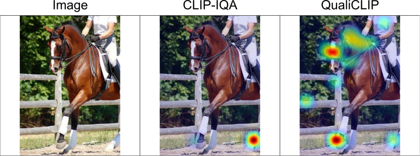
(a) Positive prompt

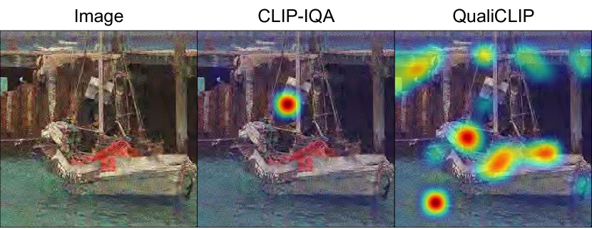
(b) Negative prompt

Figure 6: gradCAM [29] visualization of the most important regions of the input image for each of the antonym prompts. We consider the last convolutional layer of the ResNet50.

5 Conclusion

In this work, we observe that CLIP struggles to generate representations that correlate with the inherent quality of the images. To address this issue, we propose QualiCLIP, a self-supervised opinion-unaware approach aimed at enhancing CLIP’s ability to produce accurate quality-aware image representations. In particular, we design a quality-aware image-text alignment strategy that trains CLIP to rank increasingly synthetically degraded images based on their similarity with antonym prompts, while ensuring consistent representations for images with comparable quality. The experiments show that QualiCLIP surpasses other state-of-the-art opinion-unaware methods – with gains of up to a 20% gain – and outperforms supervised approaches in the cross-dataset setting. Moreover, our approach demonstrates stronger robustness and improved explainability than competing methods. In future work, we will investigate how the quality-aware image representations obtained by our model can help improve the performance of CLIP-based methods designed for semantic tasks, such as image retrieval.

Acknowledgments
This work was partially supported by the European Commission under European Horizon 2020 Programme, grant number 951911 - AI4Media.

Quality-aware Image-Text Alignment
for Real-World Image Quality Assessment
Supplementary Material

Table S4: Analysis of the individual prompt contributions in the quality score computation. $T_{p}$ and $T_{n}$ indicate the positive and negative prompts, respectively. Best and second-best scores are highlighted in bold and underlined, respectively.

		LIVE		TID2013
$T_{p}$	$T_{n}$	SRCC	PLCC	SRCC	PLCC
✓	✗	0.382	0.381	0.059	0.206
✗	✓	0.735	0.768	0.604	0.669
✓	✓	0.887	0.880	0.626	0.679

S6 Analysis of Individual Prompt Contributions

The results of the ablation studies on the training loss terms reported in Sec. 4.4 and Tab. 3 (left) show that $\mathcal{L}_{neg}$ is more important than $\mathcal{L}_{pos}$ in the training process. We recall that $\mathcal{L}_{pos}$ (Eq. 2) and $\mathcal{L}_{neg}$ (Eq. 3) involve the alignment between the images and the positive and negative prompts, respectively. Therefore, this finding suggests that the negative prompt contributes more than the positive one in the quality score computation (illustrated in Fig. 4). To support this hypothesis, we study the individual contribution of the positive and negative prompts in obtaining the final quality scores.

Let $T_{p}$ and $T_{n}$ be the positive and negative prompts that compose the pair of antonym prompts. We conduct an experiment where we directly use the similarity between the image and each of the antonym prompts as the quality score. This is possible because both the similarities and the quality scores are comprised between 0 and 1. Table S4 shows the results on the LIVE [30] and TID2013 [25] synthetic datasets. We observe that the similarity between the negative prompt and the image provides significantly more information about its inherent quality than using the positive prompt. This result confirms our hypothesis and is consistent with the greater importance of $\mathcal{L}_{neg}$ in our training strategy. Nevertheless, Tab. S4 also indicates that both the positive and negative prompts are crucial for the quality score computation, as the strategy illustrated in Fig. 4 achieves the best performance.

We carry out an additional experiment to investigate whether the discrepancy in the contribution between the positive and negative prompts is a result of our training strategy or is inherent to CLIP itself. Specifically, we follow the experimental setting described above to evaluate the individual contributions of the prompts in the quality score computation of CLIP-IQA [36]. We recall that CLIP-IQA employs the out-of-the-box CLIP image encoder without task-specific training and computes the quality score as depicted in Fig. 4. Our experiment reveals that $T_{p}$ and $T_{n}$ achieve a SRCC of -0.036 and 0.441 on the TID2013 dataset, respectively. This outcome leads us to conclude that the similarity with the negative prompt inherently provides more meaningful information about image quality compared to using the positive prompt. We plan to investigate more thoroughly on this finding in future work.

Table S5: Comparison between QualiCLIP and competing opinion-unaware methods on datasets with synthetic distortions. Best and second-best scores are highlighted in bold and underlined, respectively. OU indicates Opinion-Unaware version as explained in Sec. 4.3.

	LIVE		CSIQ		TID2013		KADID		Average
Method	SRCC	PLCC	SRCC	PLCC	SRCC	PLCC	SRCC	PLCC	SRCC	PLCC
NIQE [24]	0.908	0.905	0.628	0.719	0.312	0.398	0.379	0.438	0.557	0.615
IL-NIQE [40]	0.896	0.896	0.824	0.860	0.487	0.582	0.539	0.582	0.687	0.730
CONTRIQUE-OU [23]	0.854	0.848	0.695	0.715	0.323	0.360	0.552	0.563	0.606	0.622
Re-IQA-OU [28]	0.803	0.796	0.719	0.727	0.288	0.326	0.518	0.531	0.582	0.595
ARNIQA-OU [1]	0.871	0.863	0.816	0.805	0.464	0.533	0.630	0.635	0.695	0.709
CL-MI [4]	0.748	0.732	0.588	0.589	0.253	0.316	0.506	0.513	0.524	0.538
CLIP-IQA [36]	0.663	0.663	0.723	0.781	0.504	0.600	0.480	0.485	0.593	0.632
GRepQ-OU [32]	0.727	0.717	0.692	0.706	0.402	0.550	0.423	0.471	0.561	0.611
QualiCLIP	0.887	0.880	0.772	0.812	0.626	0.679	0.655	0.660	0.735	0.758

S7 Additional Experimental Results

S7.1 Quantitative Results

We report additional quantitative results, following the evaluation protocol detailed in Sec. 4.3. In particular, we consider synthetic datasets in the zero-shot setting, while we employ the CLIVE dataset [6] to train the baselines in the cross-dataset setting.

Zero-shot setting We evaluate the performance of our approach on four synthetically degraded datasets: LIVE [30], CSIQ [12], TID2013 [25], and KADID [15]. LIVE comprises 779 images degraded with 5 different distortion types at 5 levels of intensity, with 29 reference images as the base. CSIQ originates from 30 reference images, each distorted with 6 distinct degradations at 5 intensity levels, resulting in 866 images. TID2013 and KADID comprise 3000 and 10125 images degraded using 24 and 25 types of distortion across 5 different degrees of intensity, originating from 25 and 81 reference images, respectively. We recall that we use LIVE and TID2013 for validation, so the results of our method could likely exhibit some bias. Still, we report them for completeness. We provide the results in Tab. S5. Although primarily designed for use with authentically distorted images in real-world scenarios, QualiCLIP also achieves state-of-the-art performance on synthetic datasets. Indeed, similar to what we observed for the authentic datasets in Sec. 4.3, our method obtains significant improvements over all the baselines.

Cross-dataset setting Table S6 shows the results for the cross-dataset setting when using the CLIVE [6] dataset for training the baselines. Despite being the only opinion-unaware approach, QualiCLIP outperforms all competing approaches. In particular, our method achieves superior performance compared with other CLIP-based approaches, namely CLIP-IQA [36] and GRepQ [32]. This outcome aligns with the results reported in Tab. 2 and further confirms the effectiveness of our quality-aware image-text alignment strategy.

Table S6: Comparison between QualiCLIP and supervised methods trained on CLIVE [6]. We report the performance on several datasets with authentic distortions. Best and second-best scores are highlighted in bold and underlined, respectively.

		KonIQ		FLIVE		SPAQ		Average
Method	Opinion-Unaware	SRCC	PLCC	SRCC	PLCC	SRCC	PLCC	SRCC	PLCC
HyperIQA [33]	✗	0.750	0.787	0.335	0.483	0.776	0.796	0.620	0.689
TReS [7]	✗	0.738	0.766	0.356	0.477	0.865	0.870	0.653	0.704
CONTRIQUE [23]	✗	0.734	0.747	0.355	0.465	0.840	0.850	0.643	0.687
Re-IQA [28]	✗	0.732	0.753	0.341	0.449	0.823	0.832	0.632	0.678
ARNIQA [1]	✗	0.751	0.781	0.384	0.480	0.862	0.872	0.666	0.711
CLIP-IQA+ [36]	✗	0.780	0.814	0.369	0.481	0.855	0.861	0.668	0.719
GRepQ [32]	✗	0.779	0.793	0.345	0.449	0.839	0.852	0.654	0.698
QualiCLIP	✓	0.815	0.837	0.393	0.496	0.843	0.855	0.684	0.729

S7.2 gMAD Competition

We compare the robustness of QualiCLIP with CLIP-IQA [36] by conducting the group maximum differentiation (gMAD) competition [21]. We provide more details on gMAD in Sec. 4.5. Figure S7 shows the results. When QualiCLIP is fixed (Fig. 7(a)), CLIP-IQA struggles to identify image pairs with an evident quality gap. In contrast, when QualiCLIP operates as the attacker (Fig. 7(b)), it successfully highlights the failures of CLIP-IQA by finding image pairs displaying significantly different quality. This result shows that our approach demonstrates greater robustness than CLIP-IQA.

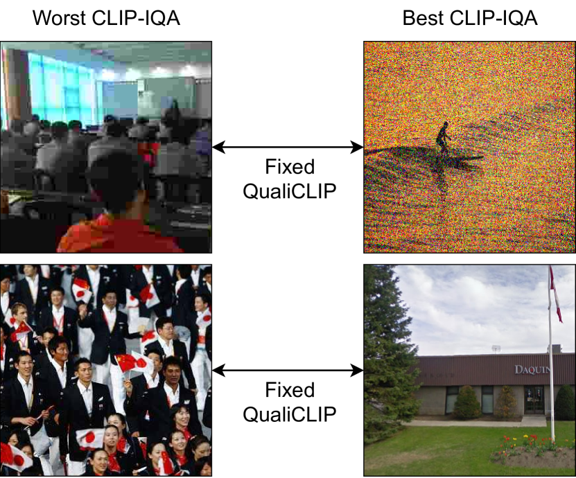
(a)

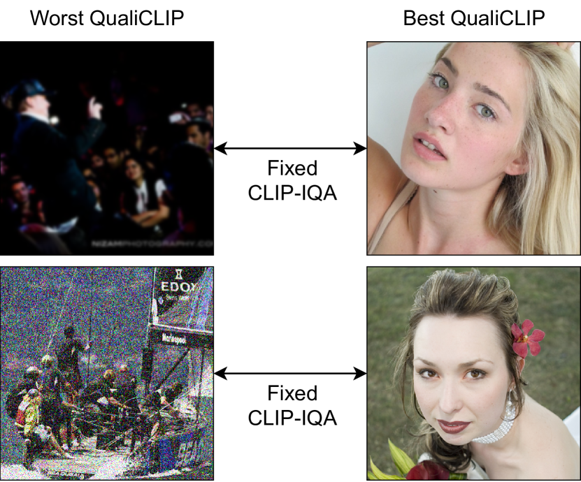
(b)

Figure S7: gMAD [21] competition results between QualiCLIP and CLIP-IQA [36]. (a): Fixed QualiCLIP at a low- (top) and high-quality (bottom) level, respectively. (b): Fixed CLIP-IQA at a low- (top) and high-quality (bottom) level, respectively.

S7.3 t-SNE Visualization

We compare the image representations generated by QualiCLIP and CLIP-IQA [36] via a t-SNE [22] visualization. Following [32], we consider images from the CLIVE [6] dataset with very high or very low quality. In particular, we take into account images with a labeled MOS greater than 75 and lower than 25, respectively. Figure S8 shows the results. We observe that the representations of high- and low-quality images obtained by the proposed approach (Fig. S8) correspond to more easily separable clusters compared to those of CLIP-IQA (Fig. S8), which are more intertwined. This result confirms that QualiCLIP generates image representations that better correlate with their intrinsic quality.

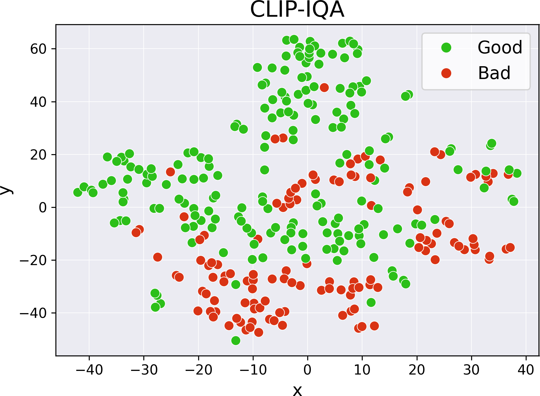
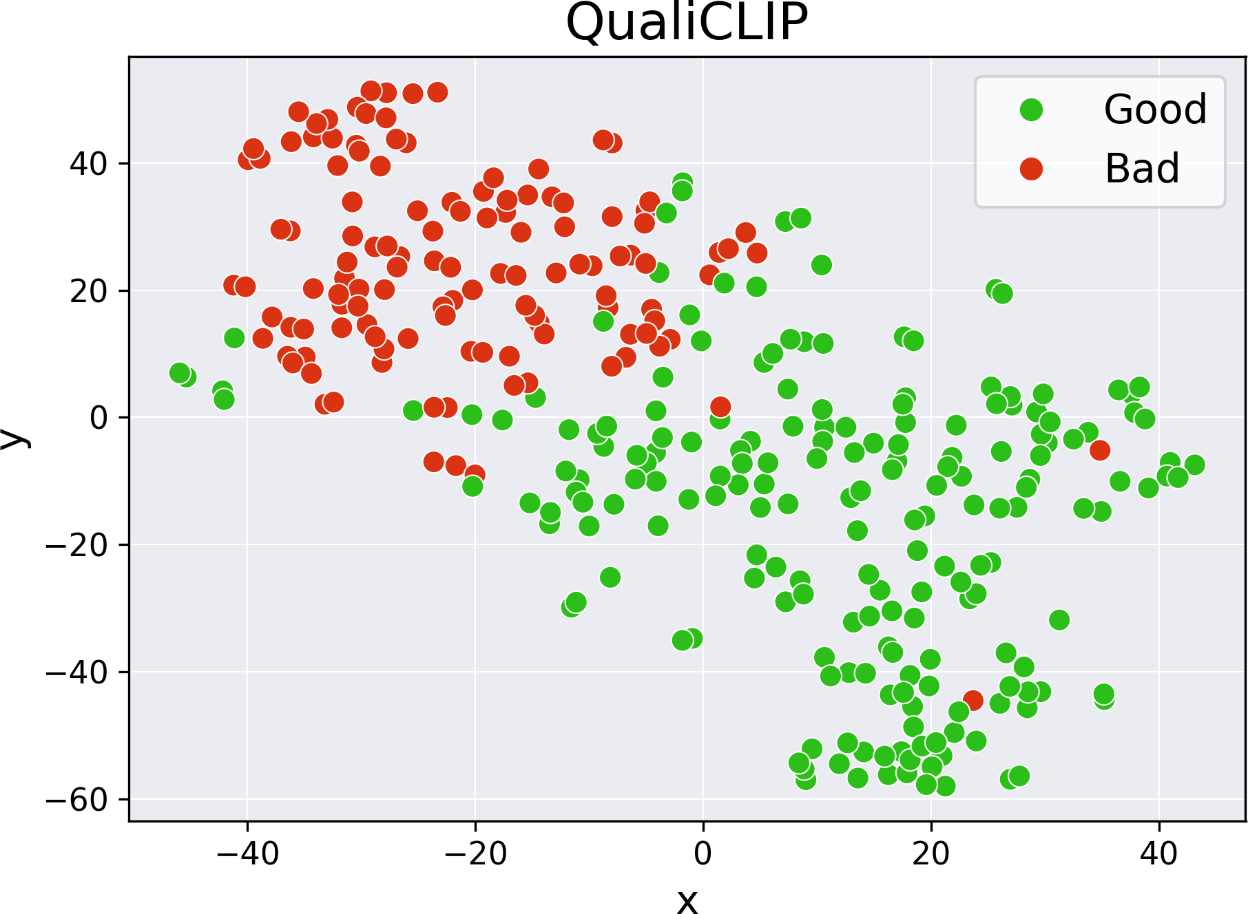
Figure S8: Comparison of the t-SNE visualizations related to the image representations of the CLIVE dataset generated by CLIP-IQA and QualiCLIP, respectively. Good and bad points refer to images with a MOS greater than 75 and lower than 25, respectively.

S8 Additional Implementation Details

S8.1 Prompts

Following [37, 38], we employ multiple pairs of antonym prompts during training and inference. In particular, we use: 1) “Good/Bad photo”; 2) “Good/Bad picture”; 3) “High-resolution/Low-resolution image”; 4) “High-quality/Low-quality image”; 5) “Sharp/Blurry image”; 6) “Sharp/Blurry edges”; 7) “Noise-free/Noisy image”. We average the similarities between the images and the pairs of prompts. As we keep the CLIP text encoder fixed, computing the text features of the prompts is a one-time requirement. Subsequently, we can employ them both for training and inference.

S8.2 Synthetic Distortions

As detailed in Sec. 3.2, during training we synthetically degrade pristine images with increasing intensity levels to make our approach self-supervised. Specifically, similar to [1] we consider 24 distinct distortion types divided into the 7 degradation groups defined by the KADID [15] dataset. Each degradation has 5 degrees of progressively higher intensity. We report an example for all the intensity levels of each distortion belonging to the degradation groups in Figs. S9, S10, S11, S12, S13, S14 and S15. Each distortion is described as follows:

1. Brightness change:

   • Brighten: applies a sequence of color space transformations, curve adjustments, and blending operations to increase the brightness of the image;

   • Darken: similar to the brighten operation, but reduces the brightness instead of increasing it;

   • Mean shift: adjusts the average intensity of image pixels by adding a constant value to all pixel values. Then, it constrains the resulting values to stay within the original image range;

2. Blur:

   • Gaussian blur: applies a Gaussian kernel filter to each image pixel;

   • Lens blur: applies a circular kernel filter to each image pixel;

   • Motion blur: applies a linear motion blur kernel to each image pixel, simulating the effect of either a moving camera or a moving object in the scene. This results in the image appearing blurred in the direction of the motion;

3. Spatial distortions:

   • Jitter: randomly displaces image data by applying small offsets to warp each pixel;

   • Non-eccentricity patch: randomly selects patches from the image and places them in random neighboring positions;

   • Pixelate: employs a combination of downscaling and upscaling operations using nearest-neighbor interpolation;

   • Quantization: quantizes the image into $N$ uniform levels. The quantization thresholds are dynamically computed using Multi-Otsu’s method [14];

   • Color block: randomly superimposes uniformly colored square patches onto the image;

4. Noise:

   • White noise: adds Gaussian white noise to the image;

   • White noise in color component: transforms the image to the YCbCr color space and then adds Gaussian white noise to each channel;

   • Impulse noise: adds salt and pepper noise to the image;

   • Multiplicative noise: adds speckle noise to the image;

5. Color distortions:

   • Color diffusion: transforms the image to the LAB color space and then applies Gaussian blur to each channel;

   • Color shift: randomly shifts the green channel and then blends it into the original image, masking it with the normalized gradient magnitude of the original image;

   • Color saturation 1: transforms the image to the HSV color space and then scales the saturation channel by a factor;

   • Color saturation 2: transforms the image to the LAB color space and then scales each color channel by a factor;

6. Compression:

   • JPEG2000: applies the standard JPEG2000 compression to the image;

   • JPEG: applies the standard JPEG compression to the image;

7. Sharpness & contrast:

   • High sharpen: applies unsharp masking to sharpen the image in the LAB color space;

   • Nonlinear contrast change: applies a nonlinear tone mapping operation to adjust the contrast of the image;

   • Linear contrast change: applies a linear tone mapping operation to adjust the contrast of the image;

	Level 1	Level 2	Level 3	Level 4	Level 5
Brighten
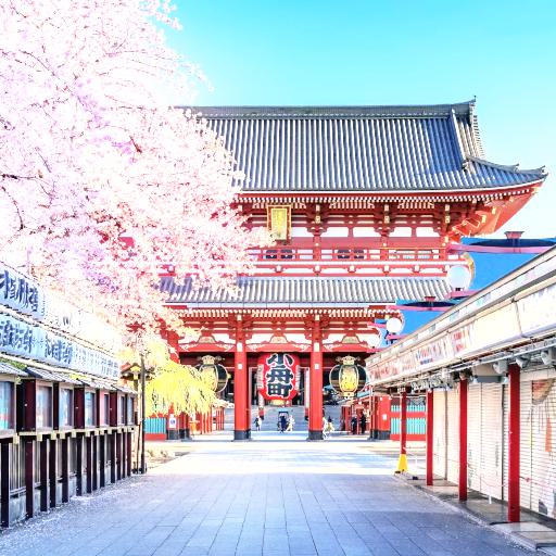
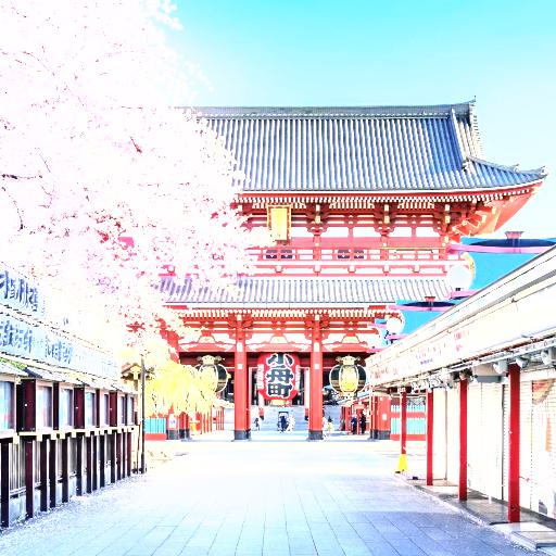
Darken
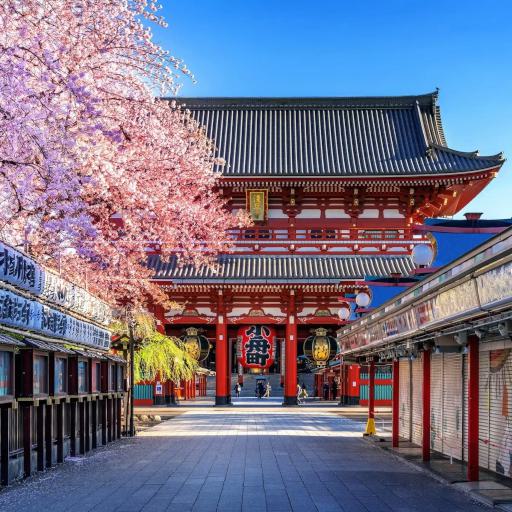
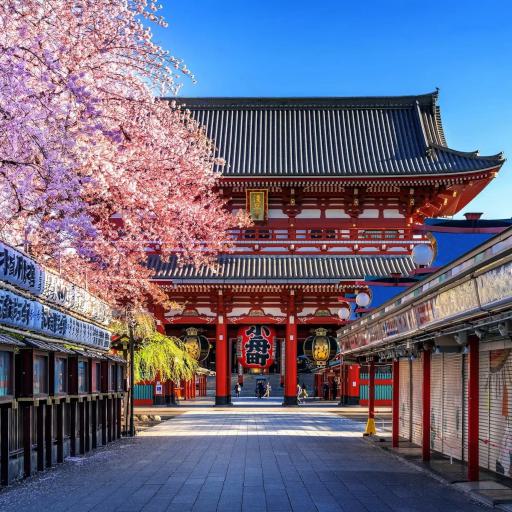
Mean shift

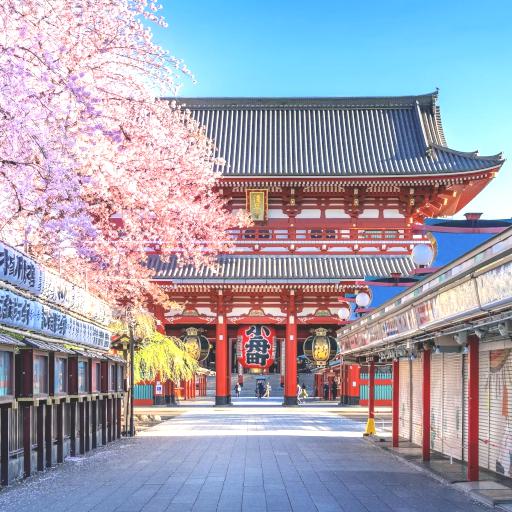
Figure S9: Visualization of the distortion types belonging to the Brightness change group for increasing intensity levels.

	Level 1	Level 2	Level 3	Level 4	Level 5
Gaussian blur
Lens blur
Motion blur

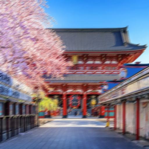
Figure S10: Visualization of the distortion types belonging to the Blur group for increasing intensity levels.

	Level 1	Level 2	Level 3	Level 4	Level 5
Jitter
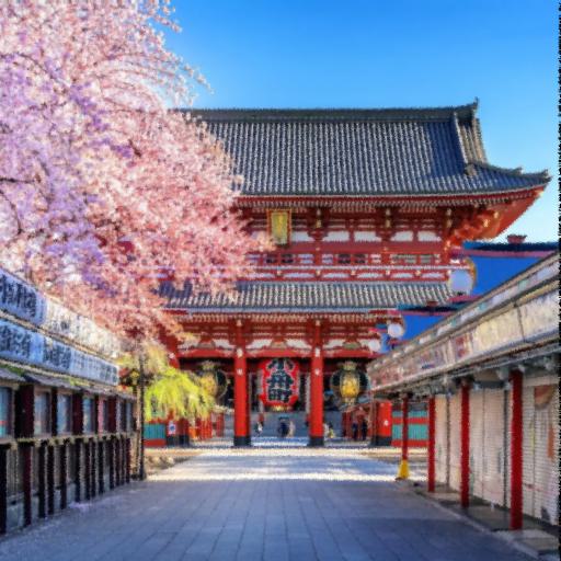
Non-eccentricity patch
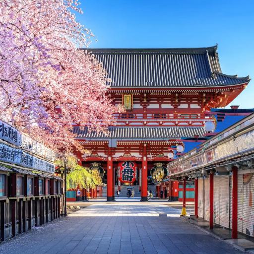
Pixelate
Quantization
Color block

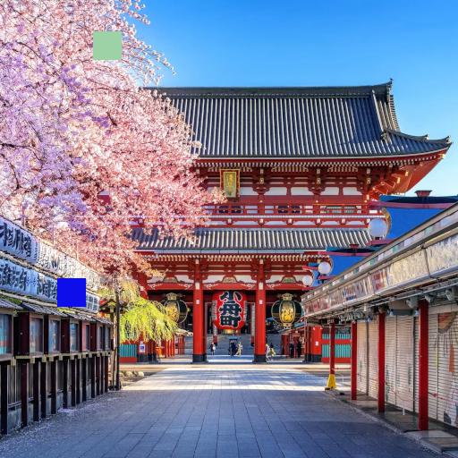
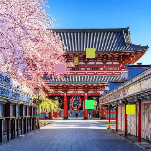
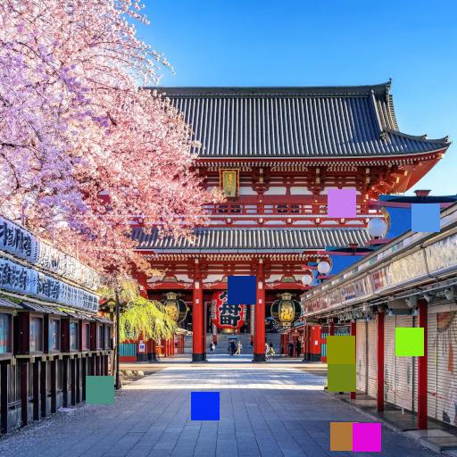
Figure S11: Visualization of the distortion types belonging to the Spatial distortions group for increasing intensity levels.

	Level 1	Level 2	Level 3	Level 4	Level 5
White noise
White noise
color
component
Impulse
noise
Multiplicative noise

Figure S12: Visualization of the distortion types belonging to the Noise group for increasing intensity levels.

	Level 1	Level 2	Level 3	Level 4	Level 5
Color diffusion
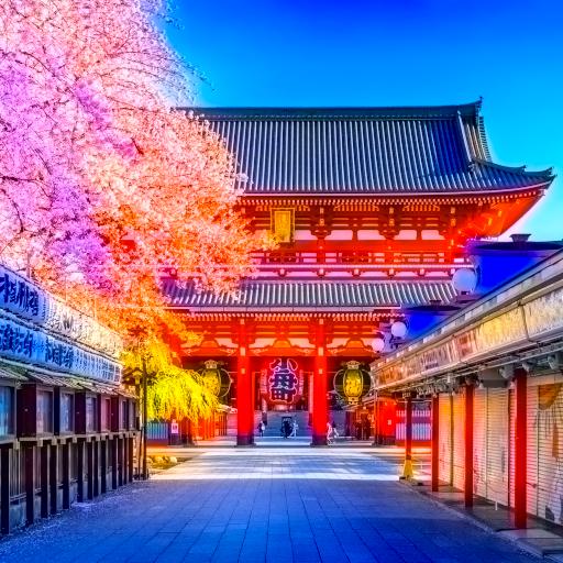
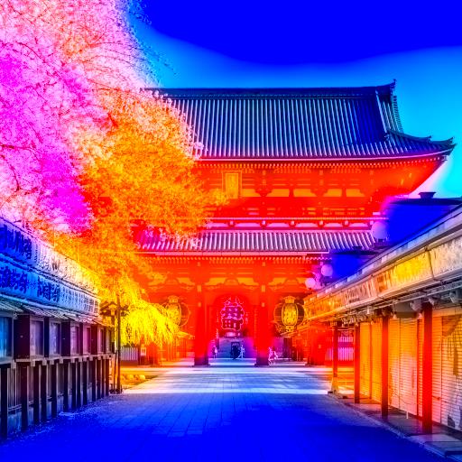
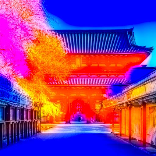
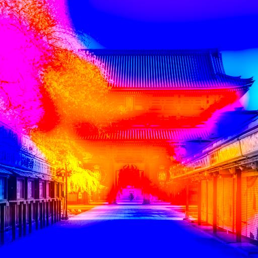
Color shift
Color saturation 1
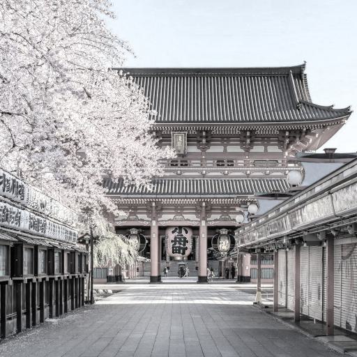
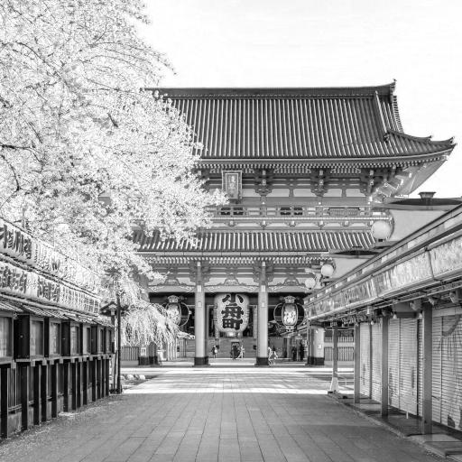
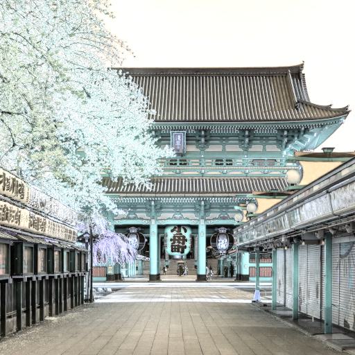
Color saturation 2

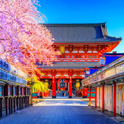
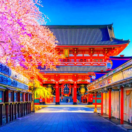
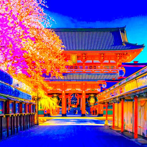
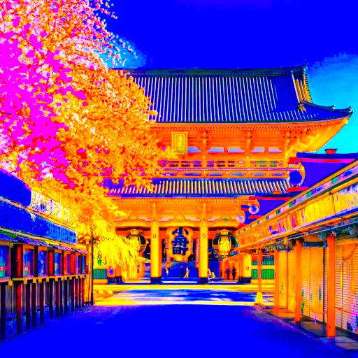
Figure S13: Visualization of the distortion types belonging to the Color distortions group for increasing intensity levels.

	Level 1	Level 2	Level 3	Level 4	Level 5
JPEG2000
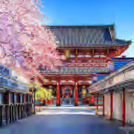
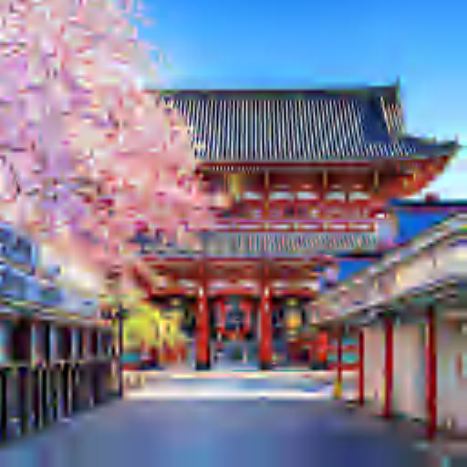
JPEG

Figure S14: Visualization of the distortion types belonging to the Compression group for increasing intensity levels.

	Level 1	Level 2	Level 3	Level 4	Level 5
High sharpen
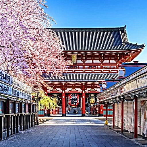
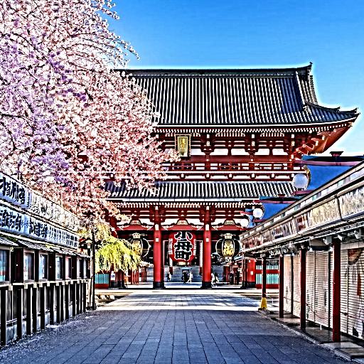
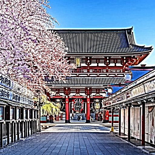
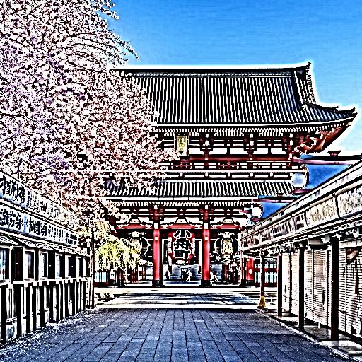
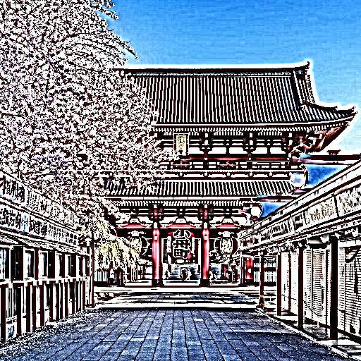
Nonlinear contrast change
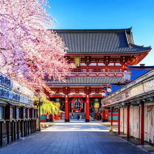
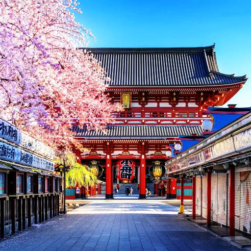
Linear contrast change

Figure S15: Visualization of the distortion types belonging to the Sharpness & contrast group for increasing intensity levels.

References

- [1] Agnolucci, L., Galteri, L., Bertini, M., Del Bimbo, A.: ARNIQA: Learning Distortion Manifold for Image Quality Assessment. In: Proceedings of the IEEE/CVF Winter Conference on Applications of Computer Vision. pp. 189–198 (2024)
- [2] Agnolucci, L., Galteri, L., Bertini, M., Del Bimbo, A.: Reference-based restoration of digitized analog videotapes. In: Proceedings of the IEEE/CVF Winter Conference on Applications of Computer Vision. pp. 1659–1668 (2024)
- [3] Antkowiak, J., Baina, T.J., Baroncini, F.V., Chateau, N., FranceTelecom, F., Pessoa, A.C.F., Colonnese, F.S., Contin, I.L., Caviedes, J., Philips, F.: Final report from the video quality experts group on the validation of objective models of video quality assessment march 2000. Final report from the video quality experts group on the validation of objective models of video quality assessment march 2000 (2000)
- [4] Babu, N.C., Kannan, V., Soundararajan, R.: No reference opinion unaware quality assessment of authentically distorted images. In: Proceedings of the IEEE/CVF Winter Conference on Applications of Computer Vision. pp. 2459–2468 (2023)
- [5] Fang, Y., Zhu, H., Zeng, Y., Ma, K., Wang, Z.: Perceptual quality assessment of smartphone photography. In: Proceedings of the IEEE/CVF Conference on Computer Vision and Pattern Recognition. pp. 3677–3686 (2020)
- [6] Ghadiyaram, D., Bovik, A.C.: Massive online crowdsourced study of subjective and objective picture quality. IEEE Transactions on Image Processing 25(1), 372–387 (2015)
- [7] Golestaneh, S.A., Dadsetan, S., Kitani, K.M.: No-reference image quality assessment via transformers, relative ranking, and self-consistency. In: Proceedings of the IEEE/CVF Winter Conference on Applications of Computer Vision. pp. 1220–1230 (2022)
- [8] Gu, J., Meng, G., Da, C., Xiang, S., Pan, C.: No-reference image quality assessment with reinforcement recursive list-wise ranking. In: Proceedings of the AAAI Conference on Artificial Intelligence. vol. 33, pp. 8336–8343 (2019)
- [9] He, K., Zhang, X., Ren, S., Sun, J.: Deep residual learning for image recognition. In: Proceedings of the IEEE conference on computer vision and pattern recognition. pp. 770–778 (2016)
- [10] Hosu, V., Lin, H., Sziranyi, T., Saupe, D.: Koniq-10k: An ecologically valid database for deep learning of blind image quality assessment. IEEE Transactions on Image Processing 29, 4041–4056 (2020)
- [11] Ke, J., Ye, K., Yu, J., Wu, Y., Milanfar, P., Yang, F.: Vila: Learning image aesthetics from user comments with vision-language pretraining. In: Proceedings of the IEEE/CVF Conference on Computer Vision and Pattern Recognition. pp. 10041–10051 (2023)
- [12] Larson, E.C., Chandler, D.M.: Most apparent distortion: full-reference image quality assessment and the role of strategy. Journal of electronic imaging 19(1), 011006–011006 (2010)
- [13] Liang, Z., Li, C., Zhou, S., Feng, R., Loy, C.C.: Iterative prompt learning for unsupervised backlit image enhancement. In: Proceedings of the IEEE/CVF International Conference on Computer Vision. pp. 8094–8103 (2023)
- [14] Liao, P.S., Chen, T.S., Chung, P.C., et al.: A fast algorithm for multilevel thresholding. J. Inf. Sci. Eng. 17(5), 713–727 (2001)
- [15] Lin, H., Hosu, V., Saupe, D.: Kadid-10k: A large-scale artificially distorted iqa database. In: 2019 Tenth International Conference on Quality of Multimedia Experience (QoMEX). pp. 1–3. IEEE (2019)
- [16] Liu, X., Van De Weijer, J., Bagdanov, A.D.: Rankiqa: Learning from rankings for no-reference image quality assessment. In: Proceedings of the IEEE international conference on computer vision. pp. 1040–1049 (2017)
- [17] Loshchilov, I., Hutter, F.: Decoupled weight decay regularization. arXiv preprint arXiv:1711.05101 (2017)
- [18] Luo, Z., Gustafsson, F.K., Zhao, Z., Sjölund, J., Schön, T.B.: Controlling vision-language models for universal image restoration. arXiv preprint arXiv:2310.01018 (2023)
- [19] Ma, K., Duanmu, Z., Wu, Q., Wang, Z., Yong, H., Li, H., Zhang, L.: Waterloo exploration database: New challenges for image quality assessment models. IEEE Transactions on Image Processing 26(2), 1004–1016 (2016)
- [20] Ma, K., Liu, W., Liu, T., Wang, Z., Tao, D.: dipiq: Blind image quality assessment by learning-to-rank discriminable image pairs. IEEE Transactions on Image Processing 26(8), 3951–3964 (2017)
- [21] Ma, K., Wu, Q., Wang, Z., Duanmu, Z., Yong, H., Li, H., Zhang, L.: Group mad competition-a new methodology to compare objective image quality models. In: Proceedings of the IEEE Conference on Computer Vision and Pattern Recognition. pp. 1664–1673 (2016)
- [22] Van der Maaten, L., Hinton, G.: Visualizing data using t-sne. Journal of machine learning research 9(11) (2008)
- [23] Madhusudana, P.C., Birkbeck, N., Wang, Y., Adsumilli, B., Bovik, A.C.: Image quality assessment using contrastive learning. IEEE Transactions on Image Processing 31, 4149–4161 (2022)
- [24] Mittal, A., Soundararajan, R., Bovik, A.C.: Making a “completely blind” image quality analyzer. IEEE Signal processing letters 20(3), 209–212 (2012)
- [25] Ponomarenko, N., Ieremeiev, O., Lukin, V., Egiazarian, K., Jin, L., Astola, J., Vozel, B., Chehdi, K., Carli, M., Battisti, F., et al.: Color image database TID2013: Peculiarities and preliminary results. In: European workshop on visual information processing (EUVIP). pp. 106–111. IEEE (2013)
- [26] Radford, A., Kim, J.W., Hallacy, C., Ramesh, A., Goh, G., Agarwal, S., Sastry, G., Askell, A., Mishkin, P., Clark, J., et al.: Learning transferable visual models from natural language supervision. In: International conference on machine learning. pp. 8748–8763. PMLR (2021)
- [27] Roy, S., Mitra, S., Biswas, S., Soundararajan, R.: Test time adaptation for blind image quality assessment. In: Proceedings of the IEEE/CVF International Conference on Computer Vision. pp. 16742–16751 (2023)
- [28] Saha, A., Mishra, S., Bovik, A.C.: Re-iqa: Unsupervised learning for image quality assessment in the wild. In: Proceedings of the IEEE/CVF Conference on Computer Vision and Pattern Recognition. pp. 5846–5855 (2023)
- [29] Selvaraju, R.R., Cogswell, M., Das, A., Vedantam, R., Parikh, D., Batra, D.: Grad-cam: Visual explanations from deep networks via gradient-based localization. In: Proceedings of the IEEE international conference on computer vision. pp. 618–626 (2017)
- [30] Sheikh, H.R., Sabir, M.F., Bovik, A.C.: A statistical evaluation of recent full reference image quality assessment algorithms. IEEE Transactions on image processing 15(11), 3440–3451 (2006)
- [31] Shukla, A., Upadhyay, A., Bhugra, S., Sharma, M.: Opinion unaware image quality assessment via adversarial convolutional variational autoencoder. In: Proceedings of the IEEE/CVF Winter Conference on Applications of Computer Vision. pp. 2153–2163 (2024)
- [32] Srinath, S., Mitra, S., Rao, S., Soundararajan, R.: Learning generalizable perceptual representations for data-efficient no-reference image quality assessment. In: Proceedings of the IEEE/CVF Winter Conference on Applications of Computer Vision. pp. 22–31 (2024)
- [33] Su, S., Yan, Q., Zhu, Y., Zhang, C., Ge, X., Sun, J., Zhang, Y.: Blindly assess image quality in the wild guided by a self-adaptive hyper network. In: Proceedings of the IEEE/CVF Conference on Computer Vision and Pattern Recognition. pp. 3667–3676 (2020)
- [34] Thomee, B., Shamma, D.A., Friedland, G., Elizalde, B., Ni, K., Poland, D., Borth, D., Li, L.J.: Yfcc100m: The new data in multimedia research. Communications of the ACM 59(2), 64–73 (2016)
- [35] Thong, W., Pereira, J.C., Parisot, S., Leonardis, A., McDonagh, S.: Content-diverse comparisons improve iqa. arXiv preprint arXiv:2211.05215 (2022)
- [36] Wang, J., Chan, K.C., Loy, C.C.: Exploring clip for assessing the look and feel of images. In: Proceedings of the AAAI Conference on Artificial Intelligence. vol. 37, pp. 2555–2563 (2023)
- [37] Wu, H., Liao, L., Hou, J., Chen, C., Zhang, E., Wang, A., Sun, W., Yan, Q., Lin, W.: Exploring opinion-unaware video quality assessment with semantic affinity criterion. arXiv preprint arXiv:2302.13269 (2023)
- [38] Wu, H., Liao, L., Wang, A., Chen, C., Hou, J., Sun, W., Yan, Q., Lin, W.: Towards robust text-prompted semantic criterion for in-the-wild video quality assessment. arXiv preprint arXiv:2304.14672 (2023)
- [39] Ying, Z., Niu, H., Gupta, P., Mahajan, D., Ghadiyaram, D., Bovik, A.: From patches to pictures (paq-2-piq): Mapping the perceptual space of picture quality. In: Proceedings of the IEEE/CVF Conference on Computer Vision and Pattern Recognition. pp. 3575–3585 (2020)
- [40] Zhang, L., Zhang, L., Bovik, A.C.: A feature-enriched completely blind image quality evaluator. IEEE Transactions on Image Processing 24(8), 2579–2591 (2015)
- [41] Zhang, W., Ma, K., Yan, J., Deng, D., Wang, Z.: Blind image quality assessment using a deep bilinear convolutional neural network. IEEE Transactions on Circuits and Systems for Video Technology 30(1), 36–47 (2018)
- [42] Zhang, W., Zhai, G., Wei, Y., Yang, X., Ma, K.: Blind image quality assessment via vision-language correspondence: A multitask learning perspective. In: Proceedings of the IEEE/CVF Conference on Computer Vision and Pattern Recognition. pp. 14071–14081 (2023)
- [43] Zhao, K., Yuan, K., Sun, M., Li, M., Wen, X.: Quality-aware pre-trained models for blind image quality assessment. In: Proceedings of the IEEE/CVF Conference on Computer Vision and Pattern Recognition. pp. 22302–22313 (2023)