Selective Hourglass Mapping for Universal Image Restoration Based on Diffusion Model

Abstract

Universal image restoration is a practical and potential computer vision task for real-world applications. The main challenge of this task is handling the different degradation distributions at once. Existing methods mainly utilize task-specific conditions (e.g., prompt) to guide the model to learn different distributions separately, named multi-partite mapping. However, it is not suitable for universal model learning as it ignores the shared information between different tasks. In this work, we propose an advanced selective hourglass mapping strategy based on diffusion model, termed DiffUIR. Two novel considerations make our DiffUIR non-trivial. Firstly, we equip the model with strong condition guidance to obtain accurate generation direction of diffusion model (selective). More importantly, DiffUIR integrates a flexible shared distribution term (SDT) into the diffusion algorithm elegantly and naturally, which gradually maps different distributions into a shared one. In the reverse process, combined with SDT and strong condition guidance, DiffUIR iteratively guides the shared distribution to the task-specific distribution with high image quality (hourglass). Without bells and whistles, by only modifying the mapping strategy, we achieve state-of-the-art performance on five image restoration tasks, 22 benchmarks in the universal setting and zero-shot generalization setting. Surprisingly, by only using a lightweight model (only 0.89M), we could achieve outstanding performance. The source code and pre-trained models are available at https://github.com/iSEE-Laboratory/DiffUIR

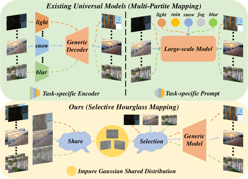
Figure 1: An illustration of existing universal image restoration methods compared with our DiffUIR, existing methods mainly design task-specific modules to handle different distributions, which force the generic model (tangerine module) to learn different distributions at once, termed multi-partite mapping. In contrast, the proposed DiffUIR maps the different distributions to one shared distribution (i.e., note that it is not the pure Gaussian distribution) while maintaining strong condition guidance. In this way, DiffUIR enables the generic model to only learn one shared distribution and guides the shared distribution to a task-specific distribution, termed selective hourglass mapping. Zoom in for best view.

1 Introduction

Universal image restoration aims to handle different image restoration tasks on a single model, which has a wide range of applications in real-world robotics navigation [3] and autonomous driving [4].

The main challenge of handling different image restoration tasks by a single model is learning various distributions simultaneously. Existing universal image restoration methods [24, 57, 40, 33, 31] mainly utilize the multi-encoder architecture or prompt the large-scale models as shown in Fig. 1. In this way, according to [63], they will learn separate mappings in one model by guiding the model to learn different distributions separately when meeting specific conditions (i.e., multi-partite mapping). Despite the strong condition guidance maintaining certain image quality, they ignore the fact that different tasks may share information that has the potential to complement and enhance the performance of the single task. For instance, in deraining dataset, rainy and foggy weather invariably occur simultaneously. Attempting to learn these two degradation types independently might fall short in addressing this scenario.

In this work, we aim to capture the shared information between different tasks for better universal image restoration learning. We replace the multi-partite mapping strategy with a novel selective hourglass mapping strategy based on conditional diffusion model, termed DiffUIR. Two novel designs make our DiffUIR non-trivial. Firstly, inspired by the RDDM [28], we explicitly fuse the condition (i.e., degraded images) into the diffusing algorithm of the diffusion model and extensively concatenate the condition with the diffusing target. In this way, DiffUIR is equipped with the ability of strong condition guidance which is similar to multi-partite mapping methods. Secondly, to achieve shared distribution mapping, we integrate a shared distribution term, named SDT into the diffusion algorithm elegantly and naturally, which gradually adjusts the weight of the condition in the algorithm. By modeling the two problems, in the forward diffusing process, DiffUIR gradually reduces the weight of the condition and the various distributions will approach one shared distribution, enabling the model to capture the shared information between tasks. Notably, we map the different distributions to an impure Gaussian distribution with slight condition left, as mentioned in [10, 27, 28], the pure Gaussian noise contains no task information, which is not conducive to good generation quality. In the reverse process, by the guidance of the strong condition and SDT, DiffUIR will gradually recover from the shared distribution into the task-specific distribution.

By only modifying the mapping strategies, without bells and whistles we outperform all of the existing universal methods by a large margin in five image restoration benchmarks. Notably, we only use the model with 36.26M parameters, which is at least 5 times less than the existing large-scale model based universal methods but with higher performance. Additionally, to meet the demand of real-world applications, we propose several light versions of our DiffUIR, the tiny version DiffUIR-T comprises only 0.89M parameters, yet it exhibits outstanding performance. To further validate the ability of our universal model, we do zero-shot generalization experiment on known task and unknown task settings, which also achieve state-of-the-art performance compared with other universal methods.

In summary, our main contributions are as follows:

$(1)$ A novel selective hourglass mapping method, DiffUIR is proposed, which can freely convert various distributions to a shared one and enable the model to learn shared information between different tasks. Moreover, equipped with strong conditions, DiffUIR guides the shared distribution to a task-specific distribution with high image quality.

$(2)$ We empirically validate that our distribution mapping strategy is a better solution for the universal image restoration task. By only changing the mapping strategy, we even outperform the universal image restoration methods based on large-scale models with only $1/5$ parameters.

$(3)$ Our DiffUIR meets the demand of real-world scenes. We outperform other universal methods in zero-shot generalization setting. Our tiny version DiffUIR-T comprised only 0.89M parameters with outstanding performance.

2 Related Work

2.1 Image Restoration.

Image restoration aims to recover a clean image from its degradation counterpart, which is a fundamental and significant computer vision field and contains various tasks, such as deraining, desnowing, low-light enhancement, debluring and dehazing, etc. Existing works [12, 65, 8, 32, 70, 51, 60, 38, 28] mainly focus on resolving one specific task with unique model designs. Although these methods achieve great performance success, they ignore the fact that in real-world applications, people prefer one model that can handle all of the degradation types. Recently some pioneers have studied on universal image restoration model and made some progress. AirNet [23] uses a module to map the different distributions into one shared distribution constrained by contrastive learning, which is hard for training and the performance is limited. IDR [71] observes that different degradation types can be divided by singular value decomposition and the clean image could be recomputed by reformulating the singular value and vector. Painter [57], ProRes [33] and DA-CLIP [31] aim to incorporate the full potential of large-scale models by prompt learning. Although they use the prior knowledge of the large-scale model, due to utilizing multi-partite mapping strategy, they only perform limited performance and require a vast number of parameters.

In this work, we propose selective hourglass mapping strategy based on conditional diffusion model, equipped the model with the ability of shared distribution mapping and strong condition guidance at once. Due to these capabilities, we achieve outstanding results without relying on a complex training pipeline or large-scale models or pre-training.

2.2 Diffusion Model

Diffusion model is a new kind of generative model which fits the distribution of the empirical data from standard Gaussian distribution based on the Markov Chain. We show the theoretical and implementation details in Appendix A. Benefiting from the strong mathematical basis and great generative quality, diffusion model is widely used in various dense computer vision tasks, such as image generation [50, 45, 14, 48, 43], image editing [9, 1, 67], image segmentation [2, 64], depth estimation [46, 74], etc. As a part of dense estimation tasks, many researchers apply the diffusion model to image restoration. RainDiffusion [62] fuses the cycle framework into the conditional diffusion model and performs well in unsupervised setting, DDNM [58] constructs an elegant identity equation, which naturally adds condition into the reverse process of diffusion model without any extra training, working greatly on linear image restoration tasks. RDDM [28] changes the diffusion direction from the target domain to the input domain, which naturally integrates the condition (i.e., degraded image) into the forward process and achieves impressive performance on several image restoration benchmarks.

The approaches above present some intriguing modifications concerning conditional constraints, achieving strong condition guidance. However, they are all not suitable for universal image restoration learning. The diffusing endpoint of the standard conditional diffusion model is the standard Gaussian noise without any task-specific context information, as mentioned in [28, 10, 27], it suffers from poor recovering quality because the condition is added in a mediated way (i.e., concatenation); RDDM [28] explicitly fuses the condition into the diffusing algorithm, achieving high image quality. However, the problem of multi-partite mapping occurs as the endpoints of different tasks are distinguishable and pertain to different distributions. In this work, we address the shortcomings of existing conditional diffusion models and achieve shared distribution mapping and strong condition modeling at the same time.

3 DiffUIR

In this section, we first explore a suitable condition mechanism of diffusion model inspired by RDDM, then we introduce our selective hourglass mapping strategy which equips the abilities of shared distribution mapping and strong condition guidance for better universal learning.

3.1 Revist the condition mechanism of RDDM

RDDM [28] follows standard T-step diffusion model [48, 14] which contains a forward process and a reverse process. In the forward process, the one-step noising could be written as Markov Chain:

$$q(I_{t}|I_{t-1},I_{res})=\mathcal{N}(I_{t};I_{t-1}+\alpha_{t}I_{res},\beta^{2}_{t}\textbf{I}),\vspace{-2mm}$$ (1)

where $I_{t}$ is the diffusing result in timestep t, $I_{res}$ is the residual of degraded image $I_{in}$ and clean image $I_{0}$: $I_{res}$ = $I_{in}$ - $I_{0}$, $\alpha_{t}$ and $\beta_{t}$ is the noise coefficient of $I_{res}$ and Gaussian noise respectively. They change the noising objective from the $I_{0}$ (i.e., used in previous image restoration diffusion methods [62, 38]) to $I_{res}$ following the residual learning [13]. By the property of Markov Chain and reparameterization [19, 20] technology, the one-step noising distribution could be extended to any step noising form as follows:

$$q(I_{t}|I_{0},I_{res})=\mathcal{N}(I_{t};I_{0}+\overline{\alpha}_{t}I_{res},\overline{\beta}_{t}\textbf{I}),\vspace{-2mm}$$ (2)

where $\overline{\alpha}_{t}=\sum_{i=1}^{t}\alpha_{i}$, $\overline{\beta}_{t}=\sqrt{\sum_{i=1}^{t}\beta^{2}_{i}}$. Notably when $t\rightarrow T$, $\overline{\alpha}_{T}=1$ and the formula could be written as $I_{T}=I_{in}+\overline{\beta}_{T}\epsilon$. It shows that the endpoint is only related to the degraded image and the added noise, naturally adding the condition to the model training. In the reverse process, RDDM uses the $q(I_{t-1}|I_{t},I_{0}^{\theta},I_{res}^{\theta})$ to simulate the true generation distribution $p_{\theta}(I_{t-1}|I_{t})$, and it could also be written as Markov Chain:

$$p_{\theta}(I_{t-1}|I_{t})=\mathcal{N}(I_{t-1};I_{0}^{\theta}+\overline{\alpha}_{t-1}I_{res}^{\theta}+\overline{\beta}_{t-1}\epsilon^{\theta},\textbf{0}\cdot\textbf{I}),\vspace{-2mm}$$ (3)

where the terms with $\theta$ mean that they are obtained based on the model output, 0 occurs as they use the deterministic implicit sampling equation following [48].

As the endpoint of the RDDM contains information of the condition (i.e., degraded image), it is a great condition mechanism of diffusion model, we call it explicit condition, what’s more, they extensively concatenate the condition with the diffusing target, benefiting of better image quality, named implicit condition. However, the strong condition mechanism in RDDM is not suitable for universal training as the condition always exists, which means they force the model to learn different degraded distributions separately, causing multi-partite mapping and the shared information between different tasks could not be captured.

3.2 Selective Hourglass Mapping

The goal of our method is to achieve strong condition guidance and shared distribution mapping at the same time. We adopt the condition mechanism of RDDM [28] and integrate a shared distribution term (SDT) into the diffusion algorithm that achieves the synergistic effect between two components. We show our variant diffusion process below.

Distribution Approaching Forward Process. In the forward process, as we adopt the condition mechanism of RDDM [28], the one-step diffusion process is: $I_{t}=I_{t-1}+\alpha_{t}I_{res}+\beta_{t}\epsilon_{t-1}.$ To further achieve shared distribution mapping, we modify the forward process as follows:

$$I_{t} =I_{t-1}+\alpha_{t}I_{res}+\beta_{t}\epsilon_{t-1}-\delta_{t}I_{in}$$ (4)

$$=I_{t-2}+(\alpha_{t}+\alpha_{t-1})I_{res}+\sqrt{\beta^{2}_{t}+\beta^{2}_{t-1}}\epsilon_{t-2}$$

$$\quad-(\delta_{t}+\delta_{t-1})I_{in}$$

$$=I_{t-3}\dots$$

$$=I_{0}+\overline{\alpha}_{t}I_{res}+\overline{\beta}_{t}\epsilon-\overline{\delta}_{t}I_{in},$$

where $\delta_{t}I_{in}$ is the SDT, $\delta$ is the shared distribution coefficient and $\overline{\delta}_{t}=\sum_{i=1}^{t}\delta_{i}$. We set the value of $\overline{\delta}_{t}$ from 0 to 0.9, which will gradually reduce the influence of the condition. When $t\rightarrow T$, $\overline{\alpha}_{T}=1$, and the formula could be rewritten as: $I_{T}=(1-\overline{\delta}_{T})I_{in}+\overline{\beta}_{T}\epsilon=0.1I_{in}+\overline{\beta}_{T}\epsilon$, which approaches an impure Gaussian distribution (we further validate it in experiment). Note that we adopt the progressive approaching strategy to fit the diffusing process of the diffusion model naturally.

Input: Clean image: $I_{0}$;

   Degraded image: $I_{in}$;

   Residual map: $I_{res}=I_{in}-I_{0}$.

1 repeat

2       $I_{0}\sim q(I_{0})$;

3       $t\sim Uniform({1,\dots,T})$;

4       $\epsilon\sim\mathcal{N}(\bm{0},\bm{I})$;

5       $I_{t}=I_{0}+\overline{\alpha}_{t}I_{res}+\overline{\beta}_{t}\epsilon-\overline{\delta}_{t}I_{in}$;

6       Take the gradient descent step on

7         $\nabla_{\theta}\|I_{res}-I_{res}^{\theta}(I_{t},I_{in},t)\|_{1}$;

8until converged;

Algorithm 1 Training.

Distribution Diffusing Reverse Process. In the reverse process (inference stage), our goal is to recover the sample from the shared distribution (i.e., $I_{T}=(1-\overline{\delta}_{T})I_{in}+\overline{\beta}_{T}\epsilon$) to the task-specific distribution. Following the DDPM [14], we use the $q(I_{t-1}|I_{t},I_{in},I_{0}^{\theta},I_{res}^{\theta})$ to simulate the distribution of $p_{\theta}(I_{t-1}|I_{t})$ and based on the Bayes’ theorem, we could calculate it as follows:

$$\ p_{\theta}(I_{t-1}|I_{t})\rightarrow q(I_{t-1}|I_{t},I_{in},I_{0}^{\theta},I_{res}^{\theta})$$ (5)

$$=q(I_{t}|I_{t-1},I_{in},I_{res}^{\theta})\frac{q(I_{t-1}|I_{0}^{\theta},I_{res}^{\theta},I_{in})}{q(I_{t}|I_{0}^{\theta},I_{res}^{\theta},I_{in})}$$

$$\propto exp\left[-\frac{1}{2}((\frac{\overline{\beta}_{t}^{2}}{\beta_{t}^{2}\overline{\beta}_{t-1}^{2}})I_{t-1}^{2}-2(\frac{I_{t}+\delta_{t}I_{in}-\alpha_{t}I_{res}^{\theta}}{\beta_{t}^{2}}\right.$$

$$\left.+\frac{I_{0}^{\theta}+\overline{\alpha}_{t-1}I_{res}^{\theta}-\overline{\delta}_{t-1}I_{in}}{\overline{\beta}_{t-1}^{2}})I_{t-1}+C(I_{t},I_{0}^{\theta},I_{res}^{\theta},I_{in}))\right].$$

As the goal of the formulation is to obtain the distribution of the $I_{t-1}$, we simplify and rearrange it into the form about the $I_{t-1}$ and $C(I_{t},I_{0}^{\theta},I_{res}^{\theta},I_{in})$ is the term unrelated with it. Then we calculate the mean $\mu_{\theta}(I_{t},t)$ and variance $\sigma_{\theta}(I_{t},t)$ of the distribution $p_{\theta}(I_{t-1}|I_{t})$ based on Eq. (LABEL:eqn:bayes):

$$\mu_{\theta}(I_{t},t)=I_{t}-\alpha_{t}I_{res}^{\theta}+\delta_{t}I_{in}-\frac{\beta^{2}_{t}}{\overline{\beta}_{t}}\epsilon^{\theta}$$ (6)

$$\sigma_{\theta}(I_{t},t)=\frac{\beta^{2}_{t}\overline{\beta}^{2}_{t-1}}{\overline{\beta}^{2}_{t}},$$

where $I_{res}^{\theta}$ is predicted by the model and $\epsilon^{\theta}$ is obtained by the $I_{res}^{\theta}$. Based on the reparameterization [19, 20] technology, if we use the sampling strategy from the DDPM [14], $I_{t-1}$ could be calculated as follows:

$$I_{t-1}=I_{t}-\alpha_{t}I_{res}^{\theta}+\delta_{t}I_{in}-\frac{\beta^{2}_{t}}{\overline{\beta}_{t}}\epsilon^{\theta}+\frac{\beta_{t}\overline{\beta}_{t-1}}{\overline{\beta}_{t}}\epsilon_{*},\vspace{-3mm}$$ (7)

where $\epsilon_{*}$ is the random Gaussian noise. In this paper, to accelerate the sampling speed, we use the sampling strategy of DDIM [48] and $I_{t-1}$ is calculated by:

$$I_{t-1}=I_{t}-\alpha_{t}I_{res}^{\theta}+\delta_{t}I_{in}.\vspace{-2mm}$$ (8)

Based on the Eq. (8), we could iteratively recover the sample from the $I_{T}$ to $I_{T-k},I_{T-2k},\dots,I_{k},I_{0}$ where k means skip steps followed DDIM [48]. The complete sampling algorithm is shown in Algorithm 2.

Note that we only present the most important steps here and the full derivation please refer to Appendix C.

Input: Degraded image: $I_{in}$.

1 $\epsilon\sim\mathcal{N}(\bm{0},\bm{I})$;

2 $I_{T}=(1-\overline{\delta}_{T})I_{in}+\overline{\beta}_{T}\epsilon$;

3 for $t=T,\dots,1$ do

4       if $t>1$

5      

6       $I_{t-1}=I_{t}-\alpha_{t}I_{res}^{\theta}(I_{t},I_{in},t)+\delta_{t}I_{in}$;

7       else

8        $I_{t-1}=I_{in}-I_{res}^{\theta}(I_{t},I_{in},t)$;

9      

10 end for

return $I_{0}$

Algorithm 2 Sampling.

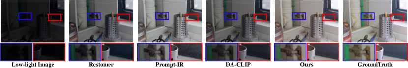
Figure 2: Visualization comparison with state-of-the-art methods on low-light enhancement. Zoom in for best view.

Universal Training Objective. We achieve universal learning by modifying the condition mechanism of diffusion model into explicit condition (injected into the diffusion algorithm) and implicit condition (concatenation) for strong condition guidance; adding SDT into the diffusion algorithm for shared distribution mapping. Although it is different from standard diffusion models [14, 48], as we both approach the different degraded distributions to one shared distribution, we reference DDPM [14] and conduct the meticulous derivation of the training objective as follows:

$$\mathcal{L}(\theta)=D_{KL}(q(I_{t-1}|I_{t},I_{0},I_{res},I_{in})||p_{\theta}(I_{t-1}|I_{t})).\vspace{-1mm}$$ (9)

As mentioned in VAE [19], the Kullback-Leibler divergence of two Gaussian distributions could be simplified to the difference of their mean, the function is transformed as:

$$\mathcal{L}(\theta) =\mathbb{E}_{q(I_{t}|I_{0})}\left[\|\mu(I_{t},I_{0})-\mu_{\theta}(I_{t},t)\|^{2}\right]$$ (10)

$$=\mathbb{E}_{t,\epsilon,I_{res}}\left[\|I_{t}-\alpha_{t}I_{res}+\delta_{t}I_{in}-\frac{\beta^{2}_{t}}{\overline{\beta}_{t}}\epsilon-\right.$$

$$\left.\quad(I_{t}-\alpha_{t}I_{res}^{\theta}+\delta_{t}I_{in}-\frac{\beta^{2}_{t}}{\overline{\beta}_{t}}\epsilon^{\theta})\|^{2}\right]$$

$$=\mathbb{E}_{t,\epsilon,I_{res}}\left[\|\alpha_{t}(I_{res}^{\theta}-I_{res})+\frac{\beta^{2}_{t}}{\overline{\beta}_{t}}(\epsilon^{\theta}-\epsilon)\|^{2}\right],$$

where $I_{res}$, $\epsilon$ mean established value in the forward process and $I_{res}^{\theta}$, $\epsilon^{\theta}$ mean predicted result in the reverse process.

Referring to the official code of DDPM [14], predicting the noise or the input is essentially equivalent, so we directly use the model to predict the residual $I_{res}^{\theta}$, the $\epsilon^{\theta}$ could be derivated by it. According to  [55, 74, 7], when predicting the input, $L_{1}$ loss performs better than $L_{2}$ loss. Based on the experimental and theoretical basis above, our final loss function is simplified as follows:

$$\mathcal{L}(\theta)_{simple}=\mathbb{E}_{t,I_{t},I_{res}}\left[\|I_{res}-I^{\theta}_{res}(I_{t},t)\|_{1}\right].\vspace{-3mm}$$ (11)

The full training algorithm is shown in Algorithm 1.

4 Experiments

4.1 Datasets and Evaluation Metrics

We evaluate the proposed DiffUIR on five image restoration tasks. We select the most widely used datasets for each task as follows, the summary table is in Appendix B:

Image deraining. We use the merged datasets mentioned in [17, 60], which covers a wide range of different rain streaks and rain density. The datasets contain 13712 data for training and 4298 data for testing, providing a robust platform to evaluate the performance of deraining methods. We further perform zero-shot generalization on real-world dataset Practical [66] which has no ground truth.

Low-light enhancement. We use the famous LOL [61] datasets as the benchmark with 485 training pairs and 15 testing pairs, which consist of a large number of indoor and outdoor scenes with different levels of light and noise. We further generalize to the widely used real-world datasets MEF [34], NPE [56] and DICM [21] without ground truth.

Image desnowing. The Snow100K [30] is used for desnowing benchmark with 50000 training data, 50000 testing data and 1329 real-world snow images. In this work, we test on Snow100K-S and Snow100K-L which means light and hazy snowflake sizes and further perform zero-shot generalization on real-world snow pairs.

Image dehazing. We use RESIDE [22] datasets as the dehazing benchmark. It is a widely used synthetic fog dataset with different hazing levels of fog and scenes. As the real-world fog condition is outdoor, we only train and test on the outdoor part with 313950 and 500 data respectively.

Image deblurring. We use the GoPro [37] dataset as the deblurring benchmark with 2103 training pairs and 1111 testing pairs. It contains various levels of blur obtained by averaging the clear images captured in very short intervals. To further validate the power of our model, we perform zero-shot generalization on HIDE [47], RealBlur-J [42] and RealBlur-R [42] with 2025, 980, 980 pairs respectively.

Table 1: Comparison of our method with other task-specific and universal image restoration approaches in five image restoration tasks. $\dagger$ means reimplementing in our datasets for fair comparison. The FLOPS is calculated in the inference stage with 256 $\times$ 256 resolution. The best results of task-specific models and universal models are shown in blue and red respectively.

Method	Year	Deraining $(5sets)$		Enhancement		Desnowing $(2sets)$		Dehazing		Deblurring		Complexity
		PSNR $\uparrow$	SSIM $\uparrow$	PSNR $\uparrow$	SSIM $\uparrow$	PSNR $\uparrow$	SSIM $\uparrow$	PSNR $\uparrow$	SSIM $\uparrow$	PSNR $\uparrow$	SSIM $\uparrow$	Params (M)	FLOPS (G)
Task-specific Method
SwinIR [25]	2021	-	-	17.81	0.723	-	-	21.5	0.891	24.52	0.773	0.9	752.13
MIRNet-v2 [70]	2022	-	-	24.74	0.851	-	-	24.03	0.927	26.30	0.799	5.9	140.92
DehazeFormer [51]	2022	-	-	-	-	-	-	34.29	0.983	-	-	4.63	48.64
Restomer [60]	2022	33.96	0.935	20.41	0.806	-	-	30.87	0.969	32.92	0.961	26.12	141
MAXIM [52]	2022	33.24	0.933	23.43	0.863	-	-	34.19	0.985	32.86	0.940	14.1	216
DRSFormer [8]	2023	33.15	0.927	-	-	-	-	-	-	-	-	33.7	242.9
IR-SDE [32]	2023	-	-	20.45	0.787	-	-	-	-	30.70	0.901	34.2	98.3
WeatherDiff [38]	2023	-	-	-	-	33.51	0.939	-	-	-	-	82.96	-
RDDM [28]$\dagger$	2023	30.74	0.903	23.22	0.899	32.55	0.927	30.78	0.953	29.53	0.876	36.26	9.88
Universal Method
Restomer$\dagger$	-	27.10	0.843	17.63	0.542	28.61	0.876	22.79	0.706	26.36	0.814	26.12	141
AirNet [23]$\dagger$	2022	24.87	0.773	14.83	0.767	27.63	0.860	25.47	0.923	26.92	0.811	8.93	30.13
Painter [57]	2022	29.49	0.868	22.40	0.872	-	-	-	-	-	-	307	248.9
IDR [71]	2023	-	-	21.34	0.826	-	-	25.24	0.943	27.87	0.846	15.34	-
ProRes [33]	2023	30.67	0.891	22.73	0.877	-	-	-	-	27.53	0.851	307	248.9
Prompt-IR [40]$\dagger$	2023	29.56	0.888	22.89	0.847	31.98	0.924	32.02	0.952	27.21	0.817	35.59	15.81
DA-CLIP [31]$\dagger$	2023	28.96	0.853	24.17	0.882	30.80	0.888	31.39	0.983	25.39	0.805	174.1	118.5
DiffUIR-T(ours)	-	28.60	0.876	23.01	0.880	30.34	0.900	30.83	0.953	27.25	0.817	0.89	1.72
DiffUIR-S(ours)	-	30.25	0.893	23.52	0.895	31.45	0.915	31.83	0.954	27.79	0.830	3.27	2.40
DiffUIR-B(ours)	-	30.56	0.901	25.06	0.900	32.37	0.924	32.70	0.956	28.54	0.851	12.41	7.19
DiffUIR-L(ours)	-	31.03	0.904	25.12	0.907	32.65	0.927	32.94	0.956	29.17	0.864	36.26	9.88

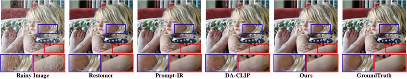
Figure 3: Visualization comparison with state-of-the-art methods on deraining. Zoom in for best view.

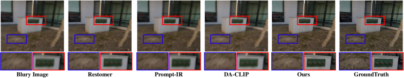
Figure 4: Visualization comparison with state-of-the-art methods on debluring. Zoom in for best view.

The benchmarks are evaluated on peak signal-to-noise ratio (PSNR) [15], structural similarity (SSIM) [59], natural image quality evaluator (NIQE) [35], lightness order error (LOE) [56], integrated local NIQE (IL -NIQE) [72] and learned perceptual image patch similarity (LPIPS) [73] metrics. Unless mentioned otherwise, PSNR and SSIM are computed using the Y channel in YCbCr color space in a way similar to existing methods [16, 69, 41, 60, 28].

4.2 Implementation Details

DiffUIR is trained from scratch using one RTX 4090 GPU with PyTorch [39] environment for 76h. During training, We use the Adam [18] optimizer and L1 loss for 300k iterations with the initial learning rate 8e-5. We set the batch sizes as 10. As the data size varies greatly from task to task, we set the weight of each task in one batch as 0.4 for dehazing, 0.1 for low-light, 0.2 for deraining, 0.2 for desnowing and 0.1 for debluring. For data augmentation, we use horizontal and vertical flips for all and preprocess the low-light data with histogram equalization. We random crop 256$\times$256 patch from the original image as network input after data augmentation for training. During inference, we test in full resolution and use 3 timesteps for all the tasks. We use U-Net [44] architecture and the hyper-parameters of our different versions are as follows:

• DiffUIR-T: $C=32$, channel multiplier = $\{1,1,1,1\}$

• DiffUIR-S: $C=32$, channel multiplier = $\{1,2,2,4\}$

• DiffUIR-B: $C=64$, channel multiplier = $\{1,2,2,4\}$

• DiffUIR-L: $C=64$, channel multiplier = $\{1,2,4,8\}$

where C is the channel number of the first hidden layers.

4.3 Evaluation on the benchmarks

We compare our DiffUIR with several task-specific methods and six universal methods on five challenge image restoration tasks. The quantitative results are shown in Table 1. We systematically analyze our method compared with other universal models below:

The necessity of universal image restoration task. We reimplement the widely known Restomer [60] in the universal setting by adding a learning prompt for each task. The result presents that directly applying the task-specific model to the universal setting is not a prudent choice.

Comparison with universal methods. We achieve outstanding performance improvement in all the tasks by a large margin (i.e., improve PSNR by 0.36 dB, 0.95 dB, 1.85 dB, 1.5 dB and 1.3 dB in Deraining, Low-light, Desnowing, Dehazing and Debluring tasks respectively), showing that selective hourglass mapping is a great solution for universal image restoration tasks. Note that we only use 1/5 parameters and 1/10 computational cost compared with other universal methods but perform outstanding performance.

Comparison under different parameters. To make a fair comparison, we provide several light versions of our DiffUIR. It could be seen that in each fair parameters level, our model outperforms the other universal models by a large margin. Notably, our DiffUIR-T comprises only 0.89M parameters, 1.72G computational cost with an outstanding performance. The great performance of different versions proves the scalability of the proposed DiffUIR.

Comparison with task-specific methods. We even achieve comparable performance compared with task-specific methods in five image restoration tasks. The phenomenon proves that different tasks contain shared information which could accelerate single-task learning.

Visual comparison. The qualitative result is shown in Fig. 2 to 4, and for more results please refer to Appendix D. It could be seen that our DiffUIR generates more steady results in all the image restoration tasks compared with other task-specific (Restomer [60]) and universal methods.

Table 2: Ablation study of each component in five image restoration tasks. EC, IC, SDT present explicit condition, implicit condition and shared distribution term respectively. We gradually remove the components to validate the synergistic effect.

Method	Condition level	Shared level	Deraining $(5sets)$		Enhancement		Desnowing $(2sets)$		Dehazing		Deblurring
			PSNR $\uparrow$	SSIM $\uparrow$	PSNR $\uparrow$	SSIM $\uparrow$	PSNR $\uparrow$	SSIM $\uparrow$	PSNR $\uparrow$	SSIM $\uparrow$	PSNR $\uparrow$	SSIM $\uparrow$
DiffUIR	Strong	Strong	31.03	0.904	25.12	0.907	32.65	0.927	32.94	0.956	29.17	0.864
-SDT	Strong	Weak	30.34	0.898	22.99	0.898	32.34	0.923	32.47	0.945	28.50	0.850
-EC & SDT	Weak	Strong	30.63	0.900	24.28	0.906	32.40	0.925	32.35	0.955	28.62	0.853
-IC & SDT	Weak	Weak	22.93	0.703	20.93	0.546	23.96	0.773	24.26	0.889	27.08	0.814

Table 3: Ablation study on shared distribution coefficient in five image restoration tasks.

Uni ratio	Deraining $(5sets)$		Enhancement		Desnowing $(2sets)$		Dehazing		Deblurring
	PSNR $\uparrow$	SSIM $\uparrow$	PSNR $\uparrow$	SSIM $\uparrow$	PSNR $\uparrow$	SSIM $\uparrow$	PSNR $\uparrow$	SSIM $\uparrow$	PSNR $\uparrow$	SSIM $\uparrow$
0.1	30.70	0.901	24.64	0.901	32.44	0.925	32.66	0.949	28.95	0.859
0.25	30.89	0.903	23.66	0.904	32.59	0.927	32.75	0.953	29.05	0.863
0.5	31.01	0.903	24.96	0.906	32.62	0.927	32.87	0.955	29.00	0.862
0.75	30.77	0.901	24.32	0.907	32.56	0.927	32.90	0.956	29.14	0.864
0.9	31.03	0.904	25.12	0.907	32.65	0.927	32.94	0.956	29.17	0.864
1	30.54	0.898	24.37	0.906	32.46	0.926	32.70	0.953	28.84	0.858

4.4 Ablation Study

We conduct ablation study on all the tasks. We first evaluate the effectiveness of the strong condition guidance and shared distribution mapping, and validate that achieving both components is necessary; then we show the effectiveness of SDT in achieving synergistic effect, and show the impact of the batch size for our universal model learning.

The synergistic effect analysis. We evaluate the effectiveness of the proposed shared distribution mapping and strong condition guidance in Table 2. We name the condition injected into the diffusion algorithm as explicit condition, the condition concatenates with the diffusing target as implicit condition. When erasing the SDT only, the model degrades to multi-partite mapping and the different distributions are not shared. The performance is impacted as the model is forced to learn different distributions separately, ignoring the shared information between different tasks; while erasing the explicit condition and SDT, the model degrades to the standard conditional diffusion model which weakens the condition level. Although it achieves shared distribution mapping, due to the mediated condition constraint, the performance drops dramatically; without the implicit condition and the SDT, the model neither provides strong condition guidance nor has shared distribution mapping and the image quality is impacted extremely. The experiments validate that equipping the model with the ability of strong condition guidance and shared distribution mapping simultaneously is significant for universal image restoration.

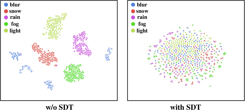
Figure 5: Distributions of the diffusing endpoint features of different image restoration tasks generated by w/o SDT and with SDT (value 0.9) visualized by t-SNE [54]. The diffusing endpoint features of different tasks are in different distributions without any interaction when without SDT. With the SDT, DiffUIR could achieve shared distribution mapping and strong condition guidance simultaneously. Zoom in for best view.

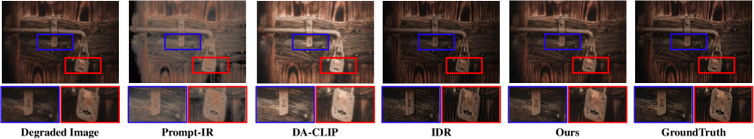
Figure 6: The visualization results of zero-shot generalization in real-world TOLED dataset. Zoom in for best view.

The effectiveness of SDT. Table 3 presents that when shared distribution coefficient is under 0.9, the performance improves with the increase of the coefficient, as the larger the coefficient, the different distributions tend to converge towards the shared distribution. While up 0.9, the performance deteriorates with the coefficient increase because the weight of the condition in the diffusion algorithm tends to 0 and the model degrades to complete shared distribution mapping (i.e., pure Gaussian distribution). The experimental result proves that our SDT and impure Gaussian distribution are significant for universal image restoration learning.

We further show the feature distributions of different tasks in Fig. 5 to show the significance of the SDT. It could be seen that by formulating the SDT into the diffusion algorithm, the different degradation distributions map to a shared one, enabling the model to capture the shared information between different tasks.

Impact of batch size. We show the result in Appendix D, the batch size is significant for our universal learning as the shared distribution mapping requires the model to sense all the tasks in the same batch.

More sampling steps. We show the result in Appendix D. Similar to other diffusion methods, DiffUIR will have a better performance with more sampling steps.

Table 4: Comparison under unknown tasks setting (under-display camera image restoration) on TOLED and POLED datasets.

Method	TOLED [75]			POLED [75]
	PSNR $\uparrow$	SSIM $\uparrow$	LPIPS $\downarrow$	PSNR $\uparrow$	SSIM $\uparrow$	LPIPS $\downarrow$
Task-specific Method
NAFNet [6]	26.89	0.774	0.346	10.83	0.416	0.794
HINet [5]	13.84	0.559	0.448	11.52	0.436	0.831
MPRNet [68]	24.69	0.707	0.347	8.34	0.365	0.798
DGUNet [36]	19.67	0.627	0.384	8.88	0.391	0.810
MIRNetV2 [70]	21.86	0.620	0.408	10.27	0.425	0.722
SwinIR [25]	17.72	0.661	0.419	6.89	0.301	0.852
RDDM [28]$\dagger$	23.48	0.639	0.383	15.58	0.398	0.544
Restomer [60]	20.98	0.632	0.360	9.04	0.399	0.742
Universal Method
DL [11]	21.23	0.656	0.434	13.92	0.449	0.756
Transweather [53]	25.02	0.718	0.356	10.46	0.422	0.760
TAPE [29]	17.61	0.583	0.520	7.90	0.219	0.799
AirNet [23]	14.58	0.609	0.445	7.53	0.350	0.820
IDR [71]	27.91	0.795	0.312	16.71	0.497	0.716
Prompt-IR [40]$\dagger$	16.70	0.688	0.422	13.16	0.583	0.619
DA-CLIP [31]$\dagger$	15.74	0.606	0.472	14.91	0.475	0.739
DiffUIR(ours)	29.55	0.887	0.281	15.62	0.424	0.505

4.5 Zero-shot generalization in real-world scenes

To evaluate the generalization ability of our DiffUIR, we do zero-shot known task generalization and unknown task generalization in real-world scenes respectively, where the difference lies in whether we know the degradation types. As our DiffUIR naturally owns the ability to handle different degradation types at once by selective hourglass mapping, we show excellent performance on both settings.

Known task generalization. As real-world datasets mainly have no ground truth, we use the perceptual evaluation metrics followed [38, 56, 71]. Table 5 shows that our DiffUIR outperforms other universal models in various benchmarks. In each degradation task, we achieve comparable or even better results with task-specific methods.

Unknown task generalization. The data [75] is obtained by under-display camera in 1024$\times$2048 resolution with various degradation types, which meets the real-world scene. The SSIM and PSNR are computed in all channels. As each image combines several degradation types, task-specific models fail in nature and as existing universal methods mainly utilize the task-specific prompt to prompt the model, the mixing degradation types confuse the model prediction. In contrast, benefiting from selective hourglass mapping, we achieve state-of-the-art performance compared with all of the methods as shown in Table 4.

Visual comparison. We show our visualization results compared with other universal methods in Fig. 6. Our method could handle low-light and blurry degradations at once benefiting from the shared distribution mapping.

4.6 Analysis of the shared distribution learning

To validate that we share useful information between different tasks, we analyze it from the perspectives below.

Theory. According to [49], adding noise will change different data from low-dimensional manifolds to high-dimensional manifolds, which learn the attributes of different data at once, validating the rationality of our method.

Visualization of the feature map. In Fig. 7, the attention of our feature map focuses on the region with rain and fog, validating that we share useful information.

Table 5: Comparison under known task generalization setting.

Method	Deraining		Enhancement		Desnowing		Deblurring
	NIQE$\downarrow$	LOE$\downarrow$	NIQE$\downarrow$	LOE$\downarrow$	NIQE$\downarrow$	IL-NIQE$\downarrow$	PSNR$\uparrow$	SSIM$\uparrow$
Task-specific Method
WeatherDiff [38]	-	-	-	-	2.96	21.976	-	-
CLIP-LIT [26]	-	-	3.70	232.48	-	-	-	-
RDDM [28]$\dagger$	3.34	41.80	3.57	202.18	2.76	22.261	30.74	0.894
Restomer [60]	3.50	30.32	3.80	351.61	-	-	32.12	0.926
Universal Method
AirNet [23]$\dagger$	3.55	145.3	3.45	598.13	2.75	21.638	16.78	0.628
Prompt-IR [40]$\dagger$	3.52	28.53	3.31	255.13	2.79	23.000	22.48	0.77
DA-CLIP [31]$\dagger$	3.52	42.03	3.56	218.27	2.72	21.498	17.51	0.667
DiffUIR(ours)	3.38	24.82	3.14	193.40	2.74	22.426	30.63	0.890

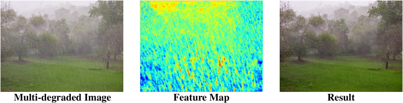
Figure 7: The visualization results of the attention of feature map during restoring multi-degraded images.

5 Conclusion

We present a selective hourglass mapping method based on conditional diffusion model, termed DiffUIR, that could achieve shared distribution mapping and strong condition guidance simultaneously for better universal image restoration learning. Specifically, we explicitly integrate the condition into the diffusion algorithm and extensively concatenate the condition to equip the model with strong condition guidance, generating accurate generation direction for diffusion model. More importantly, DiffUIR integrates a flexible shared distribution term (SDT) into the diffusion algorithm elegantly and naturally, which gradually maps different distributions into a shared one. The extensive experiments on five image restoration tasks, 22 benchmarks demonstrate that DiffUIR achieves state-of-the-art performance in the universal setting and zero-shot generalization setting compared with other universal methods.

Acknowledgments. This work was supported partially by the National Key Research and Development Program of China (2023YFA1008503), NSFC(U21A20471), Guangdong NSF Project (No. 2023B1515040025, 2020B1515120085).

References

- Avrahami et al. [2022] Omri Avrahami, Dani Lischinski, and Ohad Fried. Blended diffusion for text-driven editing of natural images. In CVPR, 2022.
- Baranchuk et al. [2021] Dmitry Baranchuk, Ivan Rubachev, Andrey Voynov, Valentin Khrulkov, and Artem Babenko. Label-efficient semantic segmentation with diffusion models. In ICLR, 2021.
- Biswas and Veloso [2011] Joydeep Biswas and Manuela Veloso. Depth camera based localization and navigation for indoor mobile robots. In RSS, 2011.
- Chen et al. [2015] Chenyi Chen, Ari Seff, Alain Kornhauser, and Jianxiong Xiao. Deepdriving: Learning affordance for direct perception in autonomous driving. In ICCV, 2015.
- Chen et al. [2021] Liangyu Chen, Xin Lu, Jie Zhang, Xiaojie Chu, and Chengpeng Chen. Hinet: Half instance normalization network for image restoration. In CVPR, 2021.
- Chen et al. [2022] Liangyu Chen, Xiaojie Chu, Xiangyu Zhang, and Jian Sun. Simple baselines for image restoration. In ECCV, 2022.
- Chen et al. [2023a] Shoufa Chen, Peize Sun, Yibing Song, and Ping Luo. Diffusiondet: Diffusion model for object detection. In ICCV, 2023a.
- Chen et al. [2023b] Xiang Chen, Hao Li, Mingqiang Li, and Jinshan Pan. Learning a sparse transformer network for effective image deraining. In CVPR, 2023b.
- Couairon et al. [2022] Guillaume Couairon, Jakob Verbeek, Holger Schwenk, and Matthieu Cord. Diffedit: Diffusion-based semantic image editing with mask guidance. In ICLR, 2022.
- Delbracio and Milanfar [2023] Mauricio Delbracio and Peyman Milanfar. Inversion by direct iteration: An alternative to denoising diffusion for image restoration. arXiv preprint arXiv:2303.11435, 2023.
- Fan et al. [2019] Qingnan Fan, Dongdong Chen, Lu Yuan, Gang Hua, Nenghai Yu, and Baoquan Chen. A general decoupled learning framework for parameterized image operators. TPAMI, 2019.
- He et al. [2010] Kaiming He, Jian Sun, and Xiaoou Tang. Single image haze removal using dark channel prior. TPAMI, 2010.
- He et al. [2016] Kaiming He, Xiangyu Zhang, Shaoqing Ren, and Jian Sun. Deep residual learning for image recognition. In CVPR, 2016.
- Ho et al. [2020] Jonathan Ho, Ajay Jain, and Pieter Abbeel. Denoising diffusion probabilistic models. In NeurIPS, 2020.
- Huynh-Thu and Ghanbari [2008] Quan Huynh-Thu and Mohammed Ghanbari. Scope of validity of psnr in image/video quality assessment. EL, 2008.
- Jiang et al. [2020a] Kui Jiang, Zhongyuan Wang, Peng Yi, Chen Chen, Baojin Huang, Yimin Luo, Jiayi Ma, and Junjun Jiang. Multi-scale progressive fusion network for single image deraining. In CVPR, 2020a.
- Jiang et al. [2020b] Kui Jiang, Zhongyuan Wang, Peng Yi, Chen Chen, Baojin Huang, Yimin Luo, Jiayi Ma, and Junjun Jiang. Multi-scale progressive fusion network for single image deraining. In CVPR, 2020b.
- Kingma and Ba [2015] Diederik P Kingma and Jimmy Ba. Adam: A method for stochastic optimization. In ICLR, 2015.
- Kingma and Welling [2014] Diederik P Kingma and Max Welling. Auto-encoding variational bayes. In ICLR, 2014.
- Kingma et al. [2019] Diederik P Kingma, Max Welling, et al. An introduction to variational autoencoders. FTML, 2019.
- Lee et al. [2012] Chulwoo Lee, Chul Lee, and Chang-Su Kim. Contrast enhancement based on layered difference representation. In ICIP, 2012.
- Li et al. [2018] Boyi Li, Wenqi Ren, Dengpan Fu, Dacheng Tao, Dan Feng, Wenjun Zeng, and Zhangyang Wang. Benchmarking single-image dehazing and beyond. TIP, 2018.
- Li et al. [2022] Boyun Li, Xiao Liu, Peng Hu, Zhongqin Wu, Jiancheng Lv, and Xi Peng. All-in-one image restoration for unknown corruption. In CVPR, 2022.
- Li et al. [2020] Ruoteng Li, Robby T Tan, and Loong-Fah Cheong. All in one bad weather removal using architectural search. In CVPR, 2020.
- Liang et al. [2021] Jingyun Liang, Jiezhang Cao, Guolei Sun, Kai Zhang, Luc Van Gool, and Radu Timofte. Swinir: Image restoration using swin transformer. In ICCV, 2021.
- Liang et al. [2023] Zhexin Liang, Chongyi Li, Shangchen Zhou, Ruicheng Feng, and Chen Change Loy. Iterative prompt learning for unsupervised backlit image enhancement. In ICCV, 2023.
- Liu et al. [2023a] Guan-Horng Liu, Arash Vahdat, De-An Huang, Evangelos A Theodorou, Weili Nie, and Anima Anandkumar. I2 sb: Image-to-image schrödinger bridge. arXiv preprint arXiv:2302.05872, 2023a.
- Liu et al. [2023b] Jiawei Liu, Qiang Wang, Huijie Fan, Yinong Wang, Yandong Tang, and Liangqiong Qu. Residual denoising diffusion models. arXiv preprint arXiv:2308.13712, 2023b.
- Liu et al. [2022] Lin Liu, Lingxi Xie, Xiaopeng Zhang, Shanxin Yuan, Xiangyu Chen, Wengang Zhou, Houqiang Li, and Qi Tian. Tape: Task-agnostic prior embedding for image restoration. In ECCV, 2022.
- Liu et al. [2018] Yun-Fu Liu, Da-Wei Jaw, Shih-Chia Huang, and Jenq-Neng Hwang. Desnownet: Context-aware deep network for snow removal. TIP, 2018.
- Luo et al. [2023a] Ziwei Luo, Fredrik K Gustafsson, Zheng Zhao, Jens Sjölund, and Thomas B Schön. Controlling vision-language models for universal image restoration. arXiv preprint arXiv:2310.01018, 2023a.
- Luo et al. [2023b] Ziwei Luo, Fredrik K Gustafsson, Zheng Zhao, Jens Sjölund, and Thomas B Schön. Image restoration with mean-reverting stochastic differential equations. ICML, 2023b.
- Ma et al. [2023] Jiaqi Ma, Tianheng Cheng, Guoli Wang, Qian Zhang, Xinggang Wang, and Lefei Zhang. Prores: Exploring degradation-aware visual prompt for universal image restoration. arXiv preprint arXiv:2306.13653, 2023.
- Ma et al. [2015] Kede Ma, Kai Zeng, and Zhou Wang. Perceptual quality assessment for multi-exposure image fusion. TIP, 2015.
- Mittal et al. [2012] Anish Mittal, Rajiv Soundararajan, and Alan C Bovik. Making a “completely blind” image quality analyzer. SPL, 2012.
- Mou et al. [2022] Chong Mou, Qian Wang, and Jian Zhang. Deep generalized unfolding networks for image restoration. In CVPR, 2022.
- Nah et al. [2017] Seungjun Nah, Tae Hyun Kim, and Kyoung Mu Lee. Deep multi-scale convolutional neural network for dynamic scene deblurring. In CVPR, 2017.
- Özdenizci and Legenstein [2023] Ozan Özdenizci and Robert Legenstein. Restoring vision in adverse weather conditions with patch-based denoising diffusion models. TPAMI, 2023.
- Paszke et al. [2019] Adam Paszke, Sam Gross, Francisco Massa, Adam Lerer, James Bradbury, Gregory Chanan, Trevor Killeen, Zeming Lin, Natalia Gimelshein, Luca Antiga, et al. Pytorch: An imperative style, high-performance deep learning library. In NeurIPS, 2019.
- Potlapalli et al. [2023] Vaishnav Potlapalli, Syed Waqas Zamir, Salman Khan, and Fahad Shahbaz Khan. Promptir: Prompting for all-in-one blind image restoration. In NeurIPS, 2023.
- Purohit et al. [2021] Kuldeep Purohit, Maitreya Suin, AN Rajagopalan, and Vishnu Naresh Boddeti. Spatially-adaptive image restoration using distortion-guided networks. In ICCV, 2021.
- Rim et al. [2020] Jaesung Rim, Haeyun Lee, Jucheol Won, and Sunghyun Cho. Real-world blur dataset for learning and benchmarking deblurring algorithms. In ECCV, 2020.
- Rombach et al. [2022] Robin Rombach, Andreas Blattmann, Dominik Lorenz, Patrick Esser, and Björn Ommer. High-resolution image synthesis with latent diffusion models. In CVPR, 2022.
- Ronneberger et al. [2015] Olaf Ronneberger, Philipp Fischer, and Thomas Brox. U-net: Convolutional networks for biomedical image segmentation. In MICCAI, 2015.
- Saharia et al. [2022] Chitwan Saharia, William Chan, Huiwen Chang, Chris Lee, Jonathan Ho, Tim Salimans, David Fleet, and Mohammad Norouzi. Palette: Image-to-image diffusion models. In SIGGRAPH, 2022.
- Shao et al. [2022] Ruizhi Shao, Zerong Zheng, Hongwen Zhang, Jingxiang Sun, and Yebin Liu. Diffustereo: High quality human reconstruction via diffusion-based stereo using sparse cameras. In ECCV, 2022.
- Shen et al. [2019] Ziyi Shen, Wenguan Wang, Xiankai Lu, Jianbing Shen, Haibin Ling, Tingfa Xu, and Ling Shao. Human-aware motion deblurring. In ICCV, 2019.
- Song et al. [2020a] Jiaming Song, Chenlin Meng, and Stefano Ermon. Denoising diffusion implicit models. In ICLR, 2020a.
- Song and Ermon [2019] Yang Song and Stefano Ermon. Generative modeling by estimating gradients of the data distribution. In NeurIPS, 2019.
- Song et al. [2020b] Yang Song, Jascha Sohl-Dickstein, Diederik P Kingma, Abhishek Kumar, Stefano Ermon, and Ben Poole. Score-based generative modeling through stochastic differential equations. In ICLR, 2020b.
- Song et al. [2023] Yuda Song, Zhuqing He, Hui Qian, and Xin Du. Vision transformers for single image dehazing. TIP, 2023.
- Tu et al. [2022] Zhengzhong Tu, Hossein Talebi, Han Zhang, Feng Yang, Peyman Milanfar, Alan Bovik, and Yinxiao Li. Maxim: Multi-axis mlp for image processing. In CVPR, 2022.
- Valanarasu et al. [2022] Jeya Maria Jose Valanarasu, Rajeev Yasarla, and Vishal M Patel. Transweather: Transformer-based restoration of images degraded by adverse weather conditions. In CVPR, 2022.
- Van der Maaten and Hinton [2008] Laurens Van der Maaten and Geoffrey Hinton. Visualizing data using t-sne. JMLR, 2008.
- Wang et al. [2023a] Hanlin Wang, Yilu Wu, Sheng Guo, and Limin Wang. Pdpp: Projected diffusion for procedure planning in instructional videos. In CVPR, 2023a.
- Wang et al. [2013] Shuhang Wang, Jin Zheng, Hai-Miao Hu, and Bo Li. Naturalness preserved enhancement algorithm for non-uniform illumination images. TIP, 2013.
- Wang et al. [2023b] Xinlong Wang, Wen Wang, Yue Cao, Chunhua Shen, and Tiejun Huang. Images speak in images: A generalist painter for in-context visual learning. In CVPR, 2023b.
- Wang et al. [2022a] Yinhuai Wang, Jiwen Yu, and Jian Zhang. Zero-shot image restoration using denoising diffusion null-space model. In ICLR, 2022a.
- Wang et al. [2004] Zhou Wang, Alan C Bovik, Hamid R Sheikh, and Eero P Simoncelli. Image quality assessment: from error visibility to structural similarity. TIP, 2004.
- Wang et al. [2022b] Zhouxia Wang, Jiawei Zhang, Runjian Chen, Wenping Wang, and Ping Luo. Restoreformer: High-quality blind face restoration from undegraded key-value pairs. In CVPR, 2022b.
- Wei et al. [2018] Chen Wei, Wenjing Wang, Wenhan Yang, and Jiaying Liu. Deep retinex decomposition for low-light enhancement. In BMVC, 2018.
- Wei et al. [2023] Mingqiang Wei, Yiyang Shen, Yongzhen Wang, Haoran Xie, and Fu Lee Wang. Raindiffusion: When unsupervised learning meets diffusion models for real-world image deraining. arXiv preprint arXiv:2301.09430, 2023.
- Xie et al. [2021] Liangbin Xie, Xintao Wang, Chao Dong, Zhongang Qi, and Ying Shan. Finding discriminative filters for specific degradations in blind super-resolution. In NeurIPS, 2021.
- Xu et al. [2023] Jiarui Xu, Sifei Liu, Arash Vahdat, Wonmin Byeon, Xiaolong Wang, and Shalini De Mello. Open-vocabulary panoptic segmentation with text-to-image diffusion models. In CVPR, 2023.
- Yang et al. [2023] Shuzhou Yang, Moxuan Ding, Yanmin Wu, Zihan Li, and Jian Zhang. Implicit neural representation for cooperative low-light image enhancement. In ICCV, 2023.
- Yang et al. [2017] Wenhan Yang, Robby T Tan, Jiashi Feng, Jiaying Liu, Zongming Guo, and Shuicheng Yan. Deep joint rain detection and removal from a single image. In CVPR, 2017.
- Yu et al. [2023] Jiwen Yu, Yinhuai Wang, Chen Zhao, Bernard Ghanem, and Jian Zhang. Freedom: Training-free energy-guided conditional diffusion model. ICCV, 2023.
- Zamir et al. [2021a] Syed Waqas Zamir, Aditya Arora, Salman Khan, Munawar Hayat, Fahad Shahbaz Khan, Ming-Hsuan Yang, and Ling Shao. Multi-stage progressive image restoration. In CVPR, 2021a.
- Zamir et al. [2021b] Syed Waqas Zamir, Aditya Arora, Salman Khan, Munawar Hayat, Fahad Shahbaz Khan, Ming-Hsuan Yang, and Ling Shao. Multi-stage progressive image restoration. In CVPR, 2021b.
- Zamir et al. [2022] Syed Waqas Zamir, Aditya Arora, Salman Khan, Munawar Hayat, Fahad Shahbaz Khan, Ming-Hsuan Yang, and Ling Shao. Learning enriched features for fast image restoration and enhancement. TPAMI, 2022.
- Zhang et al. [2023] Jinghao Zhang, Jie Huang, Mingde Yao, Zizheng Yang, Hu Yu, Man Zhou, and Feng Zhao. Ingredient-oriented multi-degradation learning for image restoration. In CVPR, 2023.
- Zhang et al. [2015] Lin Zhang, Lei Zhang, and Alan C Bovik. A feature-enriched completely blind image quality evaluator. TIP, 2015.
- Zhang et al. [2018] Richard Zhang, Phillip Isola, Alexei A Efros, Eli Shechtman, and Oliver Wang. The unreasonable effectiveness of deep features as a perceptual metric. In CVPR, 2018.
- Zheng et al. [2023] Dian Zheng, Xiao-Ming Wu, Zuhao Liu, Jingke Meng, and Wei-shi Zheng. Diffuvolume: Diffusion model for volume based stereo matching. arXiv preprint arXiv:2308.15989, 2023.
- Zhou et al. [2021] Yuqian Zhou, David Ren, Neil Emerton, Sehoon Lim, and Timothy Large. Image restoration for under-display camera. In CVPR, 2021.