Is Mamba Effective for Time Series Forecasting?

Abstract

In the realm of time series forecasting (TSF), it is imperative for models to adeptly discern and distill dependencies embedded within historical time series data. This encompasses the extraction of temporal dependencies and inter-variate correlations (VC), thereby empowering the models to forecast future states. Transformer-based models have exhibited formidable efficacy in TSF, primarily attributed to their distinct proficiency in apprehending both TD and VC. However, due to the inefficiencies, ongoing efforts to refine the Transformer persist. Recently, state space models (SSMs), e.g. Mamba, have gained traction due to their ability to process complex dependencies in sequences, similar to the Transformer, while maintaining near-linear complexity. This has piqued our interest in exploring SSM’s potential in TSF tasks. Therefore, we propose a Mamba-based model named Simple-Mamba (S-Mamba) for TSF. Specifically, we tokenize the time points of each variate autonomously via a linear layer. Subsequently, a bidirectional Mamba layer is utilized to extract VC, followed by the generation of forecast outcomes through a composite structure of a Feed-Forward Network for TD and a mapping layer. Experiments on several datasets prove that S-Mamba maintains low computational overhead and achieves leading performance. Furthermore, we conduct extensive experiments to delve deeper into the potential of Mamba compared to the Transformer in the TSF. Our code is available at https://github.com/wzhwzhwzh0921/S-D-Mamba.

Introduction

Time series forecasting (TSF) involves leveraging information from past events to predict conditions in the future. These events often have built-in patterns associated with time or variates, for example, the morning and evening peak patterns in traffic issues, and the pattern between temperature and humidity in weather predictions. This naturally leads to the consideration of identifying temporal dependencies (TD) and inter-variate correlations (VC) from these data to effectively model these patterns for better forecasting.

Transformer (Vaswani et al. 2017), which shines brightly in natural language processing (Wolf et al. 2019, 2020) and visual tasks (Liu et al. 2021; Arnab et al. 2021), is based on the self-attention structure, which can encompass the context and extract deep connections between time points in a sequence. Therefore, it is also applied in TSF tasks. Numerous Transformer-based models with impressive capabilities have been introduced (Wu et al. 2021; Zhou et al. 2022), yet the Transformer architecture faces distinct challenges. Foremost is its quadratic computational complexity, leading to a dramatic increase in calculations for long input sequences. Numerous models have attempted to reduce computational complexity by modifying the Transformer’s structure, such as focusing only on a portion of the sequence (Kitaev, Kaiser, and Levskaya 2020; Zhou et al. 2021; Li et al. 2019). However, the loss of information in this process may also lead to certain performance degradations. A more promising approach involves using linear models (Li et al. 2023a; Zeng et al. 2023), which possesses linear computational complexity. However, since they do not learn in-context and rely solely on linear numerical calculations, their performance is suboptimal compared to state-of-the-art Transformer models and accurate forecasts can only be achieved when sufficient input information is available (Zeng et al. 2023).

The State Space Models (SSM) (Gu, Goel, and Ré 2021; Smith, Warrington, and Linderman 2022) demonstrate potential in simultaneously optimizing performance and computational complexity. It employs convolutional calculation to capture sequence information and eliminates hidden states making it benefit from parallel computing and achieving near-linear complexity in processing speed. Consequently, SSM is inherently well-suited for TSF tasks. A Previous study (Rangapuram et al. 2018) also attempted to employ SSM for TSF, but the SSM architecture it used is unable to identify and filter content effectively, and the dependencies it captures are solely based on distance, resulting in unsatisfactory performance. Recent work, Mamba (Gu and Dao 2023), introduces a selective mechanism into SSM, enabling it to discern the importance of information like the attention mechanism. This development has prompted researchers to build Mamba-based models in domains where Transformer has demonstrated superior performance. The outcomes indicate that Mamba exhibits significant potential in both text and image fields, frequently achieving a win-win situation in terms of model performance and computational efficiency (Zhu et al. 2024; Yang, Xing, and Zhu 2024). This improvement is attributed to Mamba’s enhanced capability to process long sequence data, making it inherently suitable for TSF tasks and sparking our interest in exploring Mamba’s application in this field.

As a result, we launch a Mamba-based model Simple-Mamba (S-Mamba) in an attempt to reconcile the performance and speed disputes for TSF. In the S-Mamba, the time points of each variate are tokenized by a linear layer. Subsequently, a Mamba VC Encoding layer is employed to encode the VC to leverage the inter-variate mutual information for augmenting the forecasting. A FFN TD Encoding Layer containing a simple Feed-Forward Network (FFN) is followed to extract the TD. Ultimately, a mapping layer is utilized to output the forecast results. Experimental results demonstrate that S-Mamba not only achieves savings in GPU memory usage and training time but also maintains superior performance compared to state-of-the-art models. Concurrently, extensive experiments are conducted to evaluate Mamba’s efficacy and potential in TSF, for instance, to evaluate whether Mamba possesses equivalent generalization capabilities as the Transformer. Our contributions can be categorized into the following three aspects:

• We propose S-Mamba, a Mamba-based model for TSF, which delegates the extraction of inter-variate correlations and temporal dependencies to a bidirectional Mamba block and a Feed-Forward network.

• We evaluate the performance of S-Mamba, which not only has low GPU memory required and short time for forecasts but also maintains superior performance compared to the representative and state-of-the-art models.

• We conduct extensive experiments to further delve deeper into Mamba’s potential in TSF tasks.

Related Work

In conjunction with our work, two main areas of related work were investigated: (1) time series forecasting, and (2) applications of Mamba.

Time Series Forecasting

Recently, there have been two main architectures for TSF approaches, which are Transformer-based and multilayer perceptrons (MLP)-based.

Transformers are primarily designed for tasks that involve processing and generating sequences of tokens (Vaswani et al. 2017). The excellent performance of Transformer-based models has also attracted numerous researchers to focus on time series forecasting tasks (Ahmed et al. 2023). The transformer is utilized by Duong-Trung, Nguyen, and Le-Phuoc (2023) to solve the persistent challenge of long multi-horizon time series forecasting. Time Absolute Position Encoding (tAPE) and Efficient implementation of Relative Position Encoding (eRPE) are proposed in (Foumani et al. 2024) to solve the position encoding problem encountered by Transformer in multivariate time series classification (MTSC). Some researchers have also considered the application of Transformer-based time series forecasting models in specific domains, such as piezometric level prediction (Mellouli, Rabah, and Farah 2022), forecasting crude oil returns (Abdollah Pour, Hajizadeh, and Farineya 2022), predicting the power generation by solar panels (Sherozbek et al. 2023), etc.

While they excel at capturing long-range dependencies in text, they may not be as effective in modeling sequential patterns. The use of content-based attention in Transformers is not effective in detecting essential temporal dependencies, especially for time-series data with weakening dependencies over time and strong seasonality patterns (Woo et al. 2022). Particularly, the predictive capability and robustness of Transformer-based models may decrease rapidly when the input sequence is too long (Wen et al. 2023). Moreover, the $O(\text{N}^{2})$ time complexity makes Transformer-based models cost more computation and GPU memory resources. In addition, the previously mentioned issue of position encoding is also a challenge that deserves attention.

In addition to Transformer-based models, many researchers are keen to perform time series forecasting tasks using MLP-based models (Benidis et al. 2023). (Chen et al. 2023) proposed TSMixer with all-MLP architecture to efficiently utilize cross-variate and auxiliary information to improve the performance of time series forecasting. LightTS (Zhang et al. 2022) is dedicated to solving multivariate time series forecasting problems, and it can efficiently handle very long input series. (Yi et al. 2023) explores MLP in the frequency domain for time series forecasting and proposes a novel architecture for FreTS that includes two phases: domain conversion and frequency learning.

Compared to Transformer-based models, MLP-based models are simpler in structure, less complex and more efficient. However, the MLP-based models also suffer from a number of shortcomings. In the case of high volatility and non-periodic, non-stationary patterns, MLP performance relying only on past observed temporal patterns is not satisfactory (Chen et al. 2023). In other words, MLP-based models have low robustness. In addition, MLP is worse at capturing global dependencies compared to Transformers (Yi et al. 2023).

Applications of Mamba

Mamba (Gu and Dao 2023), as a new architecture, addresses to some extent the challenges faced by Transformer and MLP on time series forecasting tasks. It captures global dependencies better in a lightweight structure and has a better sense of position relationships. In addition, the Mamba architecture is more robust. Due to its excellent performance, Mamba swiftly attracted the attention of a large number of researchers. Pióro et al. (2024) replaced the Transformer architecture in the Mixture of Experts (MoE) with the Mamba architecture, achieving a complete override of Mamba’s and Transformer-MoE’s performance. Mamba has also been used to solve the long-range dependency problem in biomedical image segmentation tasks (Ma, Li, and Wang 2024). VideoMamba (Li et al. 2024) achieves efficient long-term modeling using Mamba’s linear complexity operator, showing advantages on long video understanding tasks. In addition, Mamba has demonstrated strong performance in clinical note generation (Yang et al. 2024), small target detection (Chen et al. 2024), etc.

Intuitively, the Mamba architecture can effectively mitigate the problems faced by the Transformer and MLP architectures for time series forecasting. Therefore, we try to introduce the Mamba architecture in time series forecasting tasks.

Preliminaries

Problem Statement

In time series forecasting tasks, the model receives input as a history sequence $U_{in}=[u_{1},u_{2},\ldots,u_{L}]\in{\mathbb{R}^{L\times V}}$ and $u_{n}=[p_{1},p_{2},\ldots,p_{V}]$. and then uses this information to predict a future sequence $U_{out}=[u_{L+1},u_{L+2},\ldots,u_{L+T}]\in{\mathbb{R}^{T\times V}}$. The preceding $L$ and $T$ are referred to as the review window and prediction horizon respectively, representing the lengths of the past and future time windows, while $p$ is a variate and $V$ represents the total number of variates.

State Space Models

State space models can represent any cyclical process with latent states. By using first-order differential equations to represent the evolution of the system’s internal state and another set to describe the relationship between latent states and output sequences, input sequences $x(t)\in\mathbb{R}^{D}$ can be mapped to output sequences $y(t)\in\mathbb{R}^{N}$ through latent states $h(t)\in\mathbb{R}^{N}$ in (1):

$$h(t)^{{}^{\prime}} =\textbf{\emph{A}}h(t)+\textbf{\emph{B}}x(t),$$ (1)

$$y(t) =\textbf{\emph{C}}h(t),$$

where $\textbf{\emph{A}}\in{\mathbb{R}^{N\times N}}$ and $\textbf{\emph{B,C}}\in{\mathbb{R}^{N\times D}}$ are learnable matrices. Discretize the continuous sequence using a step size $\Delta$, and the discretized SSM model is represented as (2).

$$h_{t} =\overline{\textbf{\emph{A}}}h_{t-1}+\overline{\textbf{\emph{B}}}x_{t},$$ (2)

$$y_{t} =\textbf{\emph{C}}h_{t},$$

where $\overline{\textbf{\emph{A}}}={\mathrm{exp}}(\Delta A)$ and $\overline{\textbf{\emph{B}}}=(\Delta\textbf{\emph{A}})^{-1}({\mathrm{exp}}(\Delta\textbf{\emph{A}})-I)\cdot\Delta\textbf{\emph{B}}$. Since transitioning from continuous form $(\Delta,\textbf{\emph{A}},\textbf{\emph{B}},\textbf{\emph{C}})$ to discrete form $(\overline{\textbf{\emph{A}}},\overline{\textbf{\emph{B}}},\textbf{\emph{C}})$, the model can be efficiently calculated using a linear recursive approach (Gu et al. 2021). The structured state space model (S4) (Gu, Goel, and Ré 2021), originating from the vanilla SSM, utilizes HiPPO (Gu et al. 2020) for initialization to add structure to the state matrix A, thereby improving long-range dependency modeling.

Algorithm 1 The process of Mamba Block

Input: $\bm{X}:(B,V,D)$
Output: $\bm{Y}:(B,V,D)$

1:  $x,z:(B,V,ED)\leftarrow\mathrm{Linear}(\bm{U})$ {Linear projection}

2:  $x^{{}^{\prime}}:(B,V,ED)\leftarrow\mathrm{SiLU}(\mathrm{Conv1D}(x))$

3:  $\textbf{\emph{A}}:(D,N)\leftarrow Parameter$ {Structured state matrix}

4:  $\textbf{\emph{B,C}}:(B,V,N)\leftarrow\mathrm{Linear}(x^{{}^{\prime}}),\mathrm{Linear}(x^{{}^{\prime}})$

5:  $\Delta:(B,V,D)\leftarrow\mathrm{Softplus}(Parameter+\mathrm{Broadcast}(\mathrm{Linear}(x^{{}^{\prime}})))$

6:  $\overline{\textbf{\emph{A}}},\overline{\textbf{\emph{B}}}:(B.V.D.N)\leftarrow{discretize}(\Delta,\textbf{\emph{A}},\textbf{\emph{B}})$ {Input-dependent parameters and discretization}

7:  $y:(B,V,ED)\leftarrow\mathrm{SelectiveSSM}(\overline{\textbf{\emph{A}}},\overline{\textbf{\emph{B}}},\textbf{\emph{C}})(x^{{}^{\prime}})$

8:  $y^{{}^{\prime}}:(B,V,ED)\leftarrow y\otimes\mathrm{SiLU}(z)$

9:  $\bm{Y}:(B,V,D)\leftarrow\mathrm{Linear}(y^{{}^{\prime}})$ {Linear Projection}

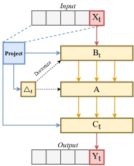
Figure 1: The structure of selective SSM (Mamba).

Mamba Block

Mamba (Gu and Dao 2023) introduces a data-dependent selection mechanism into the S4 and incorporates hardware-aware parallel algorithms in its looping mode, enabling Mamba to effectively capture contextual information in long sequences while maintaining computational efficiency. As an approximately linear perplexity series model, Mamba demonstrates significant potential in long sequence tasks, compared to transformers, in both efficiency enhancement and performance improvement. The details are presented in the algorithm related to the mamba layer in Alg.1 and the description in Fig. 1, where the former illustrates the complete data processing procedure, while the latter depicts the formation process of the output at sequence position $t$. The Mamba layer takes a sequence $\bm{X}\in\mathbb{R}^{B\times V\times D}$ as input, where $B$ denotes the batch size, $V$ denotes the number of variates, and $D$ denotes hidden dimension. The block first expands the hidden dimension to $ED$ through linear projection, obtaining $x$ and $z$. Then, it processes the projection obtained earlier using convolutional functions and a SiLU (Elfwing, Uchibe, and Doya 2017) activation function to get $x^{\prime}$. Based on the discretized SSM selected by the input parameters, denoted as the core of the mamba block, together with $x^{\prime}$, it generates the state representation $y$. Finally, $y$ is combined with a residual connection from $z$ after activation, and the final output $y_{t}$ at time step $t$ is obtained through a linear transformation. In summary, the Mamba Block effectively handles sequential information by leveraging selective state space models and input-dependent adaptations. The parameters involved in the Mamba Block include an SSM state expansion factor $N$, a size of convolutional kernel $k$, and a block expansion factor $E$ for input-output linear projection. The larger the values of $N$ and $E$, the higher the computational cost. The final output of the Mamba block is $\bm{Y}\in\mathbb{R}^{B\times V\times D}$.

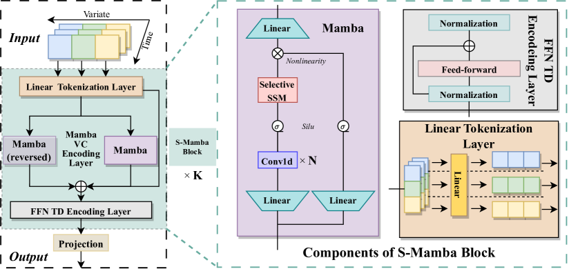
Figure 2: Overall framework of S-Mamba, the left side of the figure presents the overall architecture of our model. The right side of the figure details the components of the S-Mamba Block.

Methodology

In this section, we provide a detailed introduction of S-Mamba. Fig.2 illustrates the overall structure of S-Mamba, which is primarily composed of four layers. The first layer, the Linear Tokenization Layer, tokenizes the time series with a linear layer. The second layer, the Mamba inter-Variate correlation (VC) Encoding layer, employs a bidirectional Mamba block to capture mutual information among variates. The third layer, the FFN Temporal Dependencies (TD) Encoding Layer, further learns the temporal sequence information and finally generates future series representations by a Feed-Forward Network. Then the final layer, the Projection Layer, is only responsible for mapping the processed information of the above layers as the model’s forecast. Alg.2 demonstrates the operation process of S-Mamba.

Algorithm 2 The Forecasting Procedure of S-Mamba

Input: $Batch(U_{in})=[u_{1},u_{2},\ldots u_{L}]:(B,L,V)$
Output: $Batch(U_{out})=[u_{L+1},u_{L+2},\ldots u_{L+T}]:(B,T,V)$

1:  Linear Tokenization Layer:

2:  $Batch(U_{in}^{\top}):(B,V,L)\leftarrow\mathrm{Transpose}(Batch(U_{in}))$

3:  $\bm{U}^{tok}:(B,V,D)\leftarrow\mathrm{LinearTokenize}(Batch(U_{in}^{\top}))$ {Tokenization}

4:  for $l$ in $Mamba~{}Layers$ do

5:     Mamba VC Encoding Layer:

6:     $\overrightarrow{\bm{Y}}:(B,V,D)\leftarrow\overrightarrow{\mathrm{Mamba~{}Block}}(\bm{U})$

7:     $\overleftarrow{\bm{Y}}:(B,V,D)\leftarrow\overleftarrow{\mathrm{Mamba~{}Block}}(\bm{U})$

8:     $\bm{Y}:(B,V,D)\leftarrow\overrightarrow{\bm{Y}}+\overleftarrow{\bm{Y}}$ {Fusion Bidirectional Information}

9:     $\bm{U}^{{}^{\prime}}:(B,V,D)\leftarrow\bm{Y}+\bm{U}$ {Residual Connection}

10:     FFN TD Encoding Layer:

11:     $\bm{U}^{{}^{\prime}}:(B,V,D)\leftarrow\mathrm{LayerNorm}(\bm{U}^{{}^{\prime}})$

12:     $\bm{U}^{{}^{\prime}}:(B,V,D)\leftarrow\mathrm{Feed-Forward}(\bm{U}^{{}^{\prime}})$

13:     $\bm{U}^{{}^{\prime}}:(B,V,D)\leftarrow\mathrm{LayerNorm}(\bm{U}^{{}^{\prime}})$

14:  end for

15:  Projection:

16:  $\bm{U}^{{}^{\prime}}:(B,V,T)\leftarrow\mathrm{Projection}(\bm{U}^{{}^{\prime}})$

17:  $Batch(U_{out}):(B,T,V)\leftarrow\mathrm{Transpose}(\bm{U}^{{}^{\prime}})$

Linear Tokenization Layer

The input for the Embedding layer is $U_{in}$. Similar to iTransformer (Liu et al. 2023), we commence by tokenizing the time series, a method analogous to the tokenization of sequential text in natural language processing, to standardize the temporal series format. This pivotal task is executed by a single linear layer (3).

$$\bm{U}=\mathrm{Linear}(Batch(U_{in}))$$ (3)

where $\bm{U}$ is the output of this layer.

Mamba VC Encoding Layer

Within this layer, our primary objective is to extract the VC by linking variates that exhibit analogous trends aiming to learn the mutual information therein, thereby enabling a more robust representation of variates. The Transformer architecture confers the capacity for global attention (Vaswani et al. 2017), enabling the computation of the impact of all other variables upon a given variable, which facilitates the learning of precise information. Nonetheless, with an escalation in the number of variables, the computational burden of this global attention—characterized by its quadratic complexity—becomes untenable. In contrast, Mamba’s selective mechanism can discern the significance of different variables akin to an attention mechanism, and it exhibits a computational overhead that escalates in a near-linear fashion with an increasing count of variables. Yet, the unilateral nature of Mamba precludes it from attending to global variables in the manner of the Transformer; its selection mechanism is unidirectional, capable only of incorporating antecedent variables. To surmount this limitation, we employ two Mamba blocks to be combined as a bidirectional Mamba layer (4), which facilitates the acquisition of correlations among all variables, both antecedent and subsequent.

$$\overrightarrow{\bm{Y}}=\overrightarrow{\mathrm{Mamba~{}Block}}(\bm{U})$$ (4)

$$\overleftarrow{\bm{Y}}=\overleftarrow{\mathrm{Mamba~{}Block}}(\bm{U})$$

The VC encoded by the bidirectional Mamba is aggregated $\bm{Y}=\overrightarrow{\bm{Y}}+\overleftarrow{\bm{Y}}$ and connected with another residual network to form the output of this layer $\bm{U}^{{}^{\prime}}=\mathrm{\bm{Y}}+\bm{U}$.

FFN TD Encoding Layer

At this layer, we further process the output of the Mamba VC Encoding Layer. Firstly, we employ a normalization layer (Liu et al. 2023) to enhance convergence and training stability in deep networks by standardizing all variates to a Gaussian distribution, thereby minimizing disparities resulting from inconsistent measurements. Then, the feed-forward network (FFN) is used on the series representation of each variate. The FFN layer encodes observed time series and decodes future series representations using dense non-linear connections. During this procedure, FFN implicitly encodes TD. Finally, another normalization layer is set to adjust the future series representations as line 11-13 in Alg.1.

Projection Layer

Based on the output of the FFN TD Encoding layer, the tokenized temporal information is reconstructed into the time series requiring prediction via a mapping layer, subsequently undergoing transposition to yield the final predictive outcome.

Experiments

Datasets and Baselines

We conduct extensive experiments on several real-world datasets, including Electricity, Exchange-Rate (Lai et al. 2018), Traffic, Weather, Solar-Energy, PEMS (PEMS03, PEMS04, PEMS07, PEMS08), ETT (Electricity Transformer Temperature) (Zhou et al. 2021) (ETTh1, ETTh2, ETTm1, ETTm2). All of them are multivariate time series datasets adopted by Liu et al. (2023). Tab. 1 shows the statistics of these datasets.

Our models are fairly compared with 6 representative and state-of-the-art forecasting models, including (1) Transformer-based methods: Autoformer (Wu et al. 2021), FEDformer (Zhou et al. 2022), PatchTST (Nie et al. 2022), and (2) Linear-based methods: DLinear (Zeng et al. 2023), RLinear (Li et al. 2023b).

Table 1: The statistics of the datasets.

Datasets	Variates	Timesteps	Granularity
Electricity	321	26,304	1hour
Exchange-Rate	8	7,588	1day
Traffic	862	17,544	1hour
Weather	21	52,696	10min
Solar-Energy	137	52,560	10min
PEMS03	358	26,209	5min
PEMS04	307	16,992	5min
PEMS07	883	28,224	5min
PEMS08	170	17,856	5min
ETTm1 $\&$ ETTm2	7	17,420	15min
ETTh1 $\&$ ETTh2	7	69,680	1hour

Table 2: Full results of S-Mamba and balines. The lookback length $L$ is set to 96 and the forecast length $T$ is set to 12, 24, 48, 96 for PEMS and 96, 192, 336, 720 for other datasets. Results are averaged from all forecast lengths and full Results are in the Appendix A. The best results are highlighted in bold red font, while the second best results are presented in underlined blue font. The results of baselines are reported by Liu et al. (2023).

Models	S-Mamba		iTransformer		RLinear		PatchTST		Crossformer		TiDE		TimesNet		DLinear		FEDformer		Autoformer
Metric	MSE	MAE	MSE	MAE	MSE	MAE	MSE	MAE	MSE	MAE	MSE	MAE	MSE	MAE	MSE	MAE	MSE	MAE	MSE	MAE
ECL	0.170	0.265	0.178	0.270	0.219	0.298	0.205	0.290	0.244	0.334	0.251	0.344	0.192	0.295	0.212	0.300	0.214	0.327	0.227	0.338
Exchange	0.367	0.408	0.360	0.403	0.378	0.417	0.367	0.404	0.940	0.707	0.370	0.413	0.416	0.443	0.354	0.414	0.519	0.429	0.613	0.539
Traffic	0.414	0.276	0.428	0.282	0.626	0.378	0.481	0.304	0.550	0.304	0.760	0.473	0.620	0.336	0.625	0.383	0.610	0.376	0.628	0.379
Weather	0.251	0.276	0.258	0.278	0.272	0.291	0.259	0.281	0.259	0.315	0.271	0.320	0.259	0.287	0.265	0.317	0.309	0.360	0.338	0.382
Solar-Energy	0.240	0.273	0.233	0.262	0.369	0.356	0.270	0.307	0.641	0.639	0.347	0.417	0.301	0.319	0.330	0.401	0.291	0.381	0.885	0.711
PEMS03	0.122	0.228	0.113	0.221	0.495	0.472	0.180	0.291	0.169	0.281	0.326	0.419	0.147	0.248	0.278	0.375	0.213	0.327	0.667	0.601
PEMS04	0.103	0.211	0.111	0.221	0.526	0.491	0.195	0.307	0.209	0.314	0.353	0.437	0.129	0.241	0.295	0.388	0.231	0.337	0.610	0.590
PEMS07	0.089	0.188	0.101	0.204	0.504	0.478	0.211	0.303	0.235	0.315	0.380	0.440	0.124	0.225	0.329	0.395	0.165	0.283	0.367	0.451
PEMS08	0.148	0.224	0.150	0.226	0.529	0.487	0.280	0.321	0.268	0.307	0.441	0.464	0.193	0.271	0.379	0.416	0.286	0.358	0.814	0.659
ETTm1	0.398	0.405	0.407	0.410	0.414	0.407	0.387	0.400	0.513	0.496	0.419	0.419	0.400	0.406	0.403	0.407	0.448	0.452	0.588	0.517
ETTm2	0.288	0.332	0.288	0.332	0.286	0.327	0.281	0.326	0.757	0.610	0.358	0.404	0.291	0.333	0.350	0.401	0.305	0.349	0.327	0.371
ETTh1	0.455	0.450	0.454	0.447	0.446	0.434	0.469	0.454	0.529	0.522	0.541	0.507	0.458	0.450	0.456	0.452	0.440	0.460	0.496	0.487
ETTh2	0.381	0.405	0.383	0.407	0.374	0.398	0.387	0.407	0.942	0.684	0.611	0.550	0.414	0.427	0.559	0.515	0.437	0.449	0.450	0.459

Overall Performance

Tab.2 presents a comparative analysis of the overall performance of our models and other baseline models across all datasets. From the data presented in the table, we summarize two observations and attach the analysis: (1) S-Mamba has attained commendable outcomes on the Electricity, Traffic, PEMS, PEMS and Solar datasets. These datasets are distinguished by their numerous variates, most of which have the same period. It is worth noting that variates with the same period are more likely to contain learnable VC. Mamba VC Fusion Layer benefits from this characteristic and improves S-Mamba performance. (2) In the context of the ETT, and Exchange data sets, S-Mamba did not demonstrate a pronounced superiority in performance; indeed, it exhibited a suboptimal outcome. This can be attributed to the fact that these datasets are characterized by a limited number of variates, predominantly of an aperiodic nature. Consequently, there are weak VCs between these variates, and the employment of VC by S-Mamba may inadvertently introduce noise into the predictive model, thus impeding its predictive accuracy. (3) The Weather data set is special in that it has fewer variables and most variables are aperiodic, but S-Mamba still achieves the best performance on it.

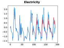
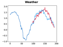
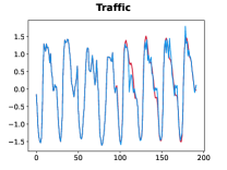
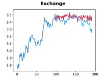
(a) S-Mamba

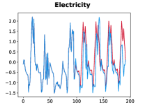
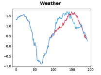
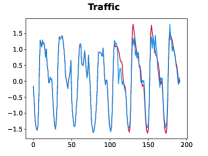
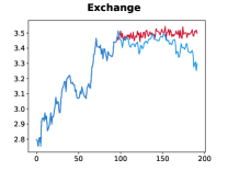
(b) iTransformer

Figure 3: Comparison of forecasts between S-Mamba and iTransformer on four datasets when the input length is 96 and the forecast length is 96. The blue line represents the ground truth and the red line represents the forecast.

Furthermore, to provide a more intuitive assessment of S-Mamba’s forecast capabilities, we visually compare the predictions of S-Mamba and the leading baseline, iTransformer, on four datasets: Electricity, Weather, Traffic, and Exchange, through graphical representation. Specifically, we randomly select a variate and then input its lookback sequence, where the true subsequent sequence is depicted as a blue line and the model’s forecast is represented by a red line in Fig.3. It is evident that on the ECL, Weather, and Traffic datasets, S-Mamba’s predictions closely approximate the actual values, with nearly perfect alignment observed on the ECL and Traffic datasets. However, on the Exchange dataset, both models exhibit relatively modest performance.

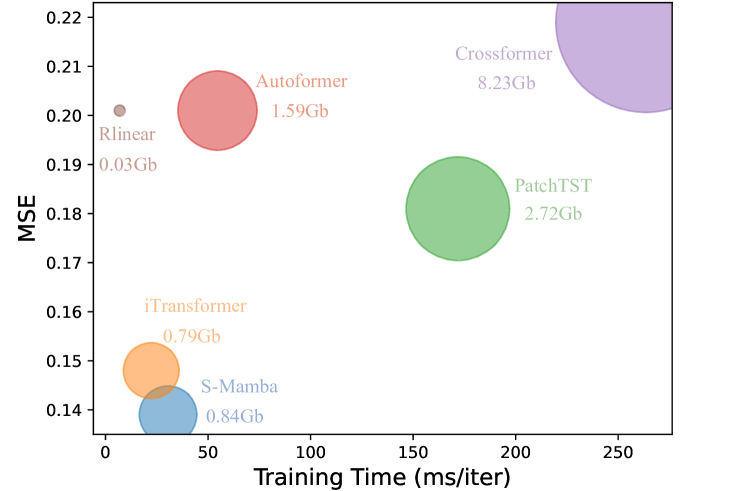
(a) Electricity

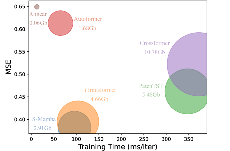
(b) Traffic

Figure 4: Comparison of S-Mamba and five baselines on MSE, Training Time, and GPU Memory.

Model Efficiency

To evaluate the computational efficiency of the models, We compare the memory usage and computing time of S-Mamba with several baselines on the ECL and Traffic. Independent runs are conducted on a single NVIDIA RTX3090 GPU and meticulously document the results in Fig.4. In our analysis, a bubble chart to depict the measurement outcomes, wherein the vertical axis denotes the Mean Squared Error (MSE), the horizontal axis quantifies the training duration, and the bubble magnitude correlates with the video memory utilization. The visualization reveals that the S-Mamba algorithm attains the most favorable MSE metric across both the Electricity and Traffic datasets. When benchmarked against Transformer-based models, S-Mamba typically necessitates a reduced training time while concurrently minimizing GPU memory consumption. While the RLinear model does utilize minimal GPU memory and curtails training time, it does not confer a competitive edge in terms of predictive precision. Overall, S-Mamba manifests exemplary predictive accuracy with a low computational resource footprint.

Table 3: Ablation study on ECL, Traffic, Weather, and Solar-Energy. The lookback length $S=96$, while the forecast length $T\in\left\{96,192,336,720\right\}$. Results are averaged from all forecast lengths.

Design	Variate	Temporal	ECL		Traffic		Weather		Solar-Energy
			MSE	MAE	MSE	MAE	MSE	MAE	MSE	MAE
S-Mamba	Mamba	FFN	0.170	0.265	0.411	0.273	0.251	0.276	0.240	0.273
Replace	Mamba	uni-Mamba	0.182	0.280	0.538	0.342	0.244	0.268	0.250	0.282
	Mamba	bi-Mamba	0.182	0.281	0.551	0.371	0.246	0.271	0.255	0.282
	Mamba	Attention	0.179	0.278	0.561	0.379	0.247	0.272	0.261	0.288
	Attention	FFN	0.178	0.270	0.428	0.282	0.258	0.279	0.233	0.262
w/o	Mamba	w/o	0.174	0.269	0.418	0.278	0.253	0.279	0.247	0.278
	w/o	FFN	0.193	0.276	0.461	0.294	0.265	0.283	0.261	0.283

Ablation Study

To evaluate the efficacy of the components within S-Mamba, we conduct ablation studies by substituting or eliminating the VC and TD encoding layers. Specifically, the VC encoding layer was replaced with an Attention mechanism or entirely removed. This modification is predicated on the empirical evidence from iTransformer experiments (Liu et al. 2023), which demonstrate that Attention was the optimal encoder for VC. Conversely, the TD encoding layer is replaced with Attention, bidirectional Mamba, unidirectional Mamba, or omitted altogether. The choice of bidirectional Mamba, which is set to benchmark Attention, is made to facilitate global temporal information extraction. The rationale behind employing unidirectional Mamba is its resemblance to RNN models, so inherently possesses the capacity to preserve sequential relationships, thereby making it a suitable candidate for evaluating the impact of sequential encoding on TD.

Our experimental investigations are conducted on four datasets: Electricity, Traffic, Weather, and Solar Energy. The findings from these experiments in Tab.6 indicate that Mamba exhibite superior performance in VC encoding, whereas the Feed-Forward Network (FFN) maintained its dominance in TD encoding.

Can Variate Order Affect Mamba’s Performance?

In the context of the S-Mamba model, the existence of the Hippo matrix (Gu et al. 2020) theoretically enables the retention of information over an indefinite length. However, this very feature predisposes the model to initially prioritize proximal information. S-Mamba employs a bidirectional Mamba layer to extract VC. This initial bias towards neighboring variates could potentially impede the acquisition of a global VC, especially when relevant variates are distant from each other. This consideration prompted us to investigate the impact of variate ordering on the performance of S-Mamba.

We hypothesize that within the dataset, variates are more likely to extract valuable information from other periodic variates. Conversely, the propensity to acquire noise increases when interacting with aperiodic variates. To address this, we apply the Fourier transform (Bracewell 1989) to help categorize variates into periodic and aperiodic groups. Our experimentation focuses on the ECL dataset, notable for its numerous periodic and aperiodic variates. The initial arrangement of these variates is depicted in the accompanying Fig.5.

Subsequent trials involve repositioning the aperiodic variates towards the middle or end of the variates sequence, followed by evaluating the predictive capabilities of the models trained on these modified datasets. For comparative analysis, we also included experiments with the iTransformer. The variate distribution and corresponding model performance are illustrated in the Fig. . Our findings suggest that the S-Mamba model’s performance remains largely unaffected by the perturbation of variate order. This implies that through adequate training, the S-Mamba can effectively mitigate the initial limitation of the Hippo matrix, which biases attention towards nearby information.

Table 4: Performance comparison between Autoformer, Flashformer and Flowformer and their variants with Mamba encoder block on ECL and Traffic datasets, where we fixed the lookback length $L=96$ and forecasting length $T=96$.

Datasets	ECL						Traffic
Models	Auto	Auto-M	Flash	Flash-M	Flow	Flow-M	Auto	Auto-M	Flash	Flash-M	Flow	Flow-M
Memory(GiB)	1.59	1.22	0.91	0.63	0.83	0.68	1.68	1.35	1.16	0.80	1.06	0.79
Speed(ms/iters)	54.6	45.1	62.8	40.6	57.4	38.0	126.1	97.3	110.3	91.5	101.5	81.2
MSE	0.201	0.191	0.253	0.252	0.252	0.246	0.613	0.607	0.68	0.67	0.658	0.649
MAE	0.317	0.305	0.347	0.345	0.349	0.344	0.338	0.381	0.374	0.465	0.360	0.365

Can Mamba Outperform Advanced Transformers?

Beyond the foundational Transformer architecture, some advanced Transformers have been introduced, predominantly focusing on the augmentation of the self-attention mechanism. We aim to determine whether Mamba can still maintain an advantage over these advanced Transformers. To this end, we conduct a comparative experiment in which we directly replace the Encoder layer of three advanced transformers: Autoformer (Wu et al. 2021), Flashformer (Dao et al. 2022) and Flowformer (Wu et al. 2022) with a unidirectional Mamba for TSF tasks to get Trans-M, Auto-M, Fed-M, Flash-M and Flow-M and and compare their performance. The results are astonishing as Tab.4, which straightforward modification with Mamba enhances the performance of these models and also reduces GPU memory usage and running time.

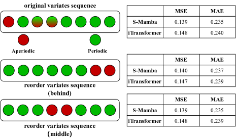
Figure 5: In the ECL dataset, adjust the distribution of periodic and aperiodic variates. The left side represents the distribution, while the right side indicates models’ performance.

Can S-Mamba Benefit from Increasing Lookback Length?

Prior research has shown that the performance of Transformer-based models does not consistently improve with increasing lookback sequence length $L$, which is somewhat unexpected. A plausible explanation is that the temporal sequence relationship is overlooked under the self-attention mechanism, as it disregards the sequential order, and in some instances, even inverts it. Mamba, resembling a Recurrent Neural Network (Medsker, Jain et al. 2001), concentrates on the preceding window during information extraction, thereby preserving certain sequential attributes. This prompts an exploration of Mamba’s potential effectiveness in temporal sequence information fusion, aiming to address the issue of diminishing or stagnant performance with increasing lookback length. Consequently, we add an additional Mamba block between the encoder Layer and decoder layer of Transformers. The role of this Mamba Block is to add a layer of time sequence dependence from the information output by the encoder layer, to add some information similar to position embedding before the decoder layer processes it. We experiment with Autoformer (Wu et al. 2021), Transformer (Vaswani et al. 2017), and Informer (Zhou et al. 2021) to get Auto-M, Infor-M, and Refor-M, and evaluate their performance with varying lookback lengths. We also test the performance of S-Mamba as the lookback length changes. The results are in the Fig.6, from which we can observe three results. (1) S-Mamba can enhance its performance as the input lengthens, but we believe this is not solely due to the Mamba Block, but rather to the Variate-based Embedding method proposed by iTransformer (Liu et al. 2023). (2) With the addition of a Mamba Block, all three models show performance improvements. Notably, the performance of Informer has seen the most significant enhancement. (3) Despite these variants’ performance gains sometimes, they do not achieve optimization with longer lookback lengths. This is consistent with the findings of Zeng et al. (2023), which also suggest that encoding temporal sequence information into the model beforehand does not resolve this issue.

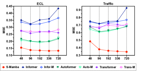
Figure 6: Forecasting performance on ECL and Traffic with the lookback length $L\in\{96,192,336,720\}$ while the prediction length $S=96$.

Is Mamba Generalizable in TSF?

The emergence of pre-trained models (Devlin et al. 2018) and large language models (Chang et al. 2023) based on the Transformer architecture has underscored the Transformer’s ability to discern similar patterns across diverse data, highlighting its generalization capabilities. In the context of TSF, it is observed that all variates exhibit a similar pattern of differences, for example, temperature and humidity in weather forecasts always have similar trends. In other words, the generalization potential of the Transformer for sequence data may also take effect on TSF tasks.

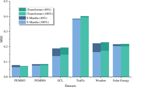
Figure 7: Forecasting performance comparison between S-Mamba and iTransformer trained on 100% variates with on 40% variates. The lookback length $L=96$ for all datasets. For the PEMS dataset, the output length $T=12$, while for the other datasets $T=96$.

In this vein, iTransformer (Liu et al. 2023) conducts a pivotal experiment. The study involves masking a majority of the variates in a dataset and training the model on a limited subset of variates. Subsequently, the model was tasked with forecasting all variates, including those previously unseen, based on the learned information from the few variates. Building on this, we seek to evaluate the generalization capabilities of Mamba in TSF tasks. An experiment is proposed wherein the S-Mamba are trained on merely 40% of the variates in the PEMS03, PEMS04, ECL, Weather, Traffic, and Solar datasets. Then they are employed to predict 100% variates, and the results are subjected to statistical analysis. The outcomes of this investigation in 7 reveal that S-Mamba exhibits generalization potential in the six datasets, which proves their generalizability in TSF tasks.

Conlusion

Transformer-based models have consistently exhibited outstanding performance in the field of time series forecasting (TSF), while Mamba has recently gained popularity, and has been shown to surpass the Transformer in various domains by delivering superior performance while reducing memory and computational overhead. Motivated by these advancements, we sought to investigate the potential of Mamba-based models in the TSF domain, with the aim of uncovering new research avenues for this field. To this end, we introduced a Mamba-based model, Simple-Mamba (S-Mamba), which transfers the task of variates information fusion from the Transformer architecture to the Mamba block. We evaluated their performance across a multitude of datasets, and our findings indicate that S-Mamba not only reduces GPU memory and computational overhead but also achieves leading performance. Furthermore, we conduct extensive experiments to prove Mamba possesses robust capabilities and exhibits remarkable potential to replace the Transformer in the TSF tasks.

Appendix A Full Results

We compare the representative and the state-of-the-art models with S-Mamba under different prediction lengths in Tab.5. The lookback length $L$ is set to 96 for all models. The number on the left side of the table represents the length of the output sequence $T$. The optimal results are highlighted in bold red font, while the suboptimal results are presented in underlined blue font. The results of baselines are reported by Liu et al. (2023).

The full results of the ablation study are represented in Tab.6.

Table 5: Full results of the long-term time series forecasting task.

Models		S-Mamba		iTransformer		RLinear		PatchTST		Crossformer		TiDE		TimesNet		DLinear		FEDformer		Autoformer
Metric		MSE	MAE	MSE	MAE	MSE	MAE	MSE	MAE	MSE	MAE	MSE	MAE	MSE	MAE	MSE	MAE	MSE	MAE	MSE	MAE
ECL	96	0.139	0.235	0.148	0.240	0.201	0.281	0.181	0.270	0.219	0.314	0.237	0.329	0.168	0.272	0.197	0.282	0.193	0.308	0.201	0.317
	192	0.159	0.255	0.162	0.253	0.201	0.283	0.188	0.274	0.231	0.322	0.236	0.330	0.184	0.289	0.196	0.285	0.201	0.315	0.222	0.334
	336	0.176	0.272	0.178	0.269	0.215	0.298	0.204	0.293	0.246	0.337	0.249	0.344	0.198	0.300	0.209	0.301	0.214	0.329	0.231	0.338
	720	0.204	0.298	0.225	0.317	0.257	0.331	0.246	0.324	0.280	0.363	0.284	0.373	0.220	0.320	0.245	0.333	0.246	0.355	0.254	0.361
Exchange	96	0.086	0.207	0.086	0.206	0.093	0.217	0.088	0.205	0.256	0.367	0.094	0.218	0.107	0.234	0.088	0.218	0.148	0.278	0.197	0.323
	192	0.182	0.304	0.177	0.299	0.184	0.307	0.176	0.299	0.470	0.509	0.184	0.307	0.226	0.344	0.176	0.315	0.271	0.315	0.300	0.369
	336	0.332	0.418	0.331	0.417	0.351	0.432	0.301	0.397	1.268	0.883	0.349	0.431	0.367	0.448	0.313	0.427	0.460	0.427	0.509	0.524
	720	0.867	0.703	0.847	0.691	0.886	0.714	0.901	0.714	1.767	1.068	0.852	0.698	0.964	0.746	0.839	0.695	1.195	0.695	1.447	0.941
Traffic	96	0.382	0.261	0.395	0.268	0.649	0.389	0.462	0.295	0.522	0.290	0.805	0.493	0.593	0.321	0.650	0.396	0.587	0.366	0.613	0.388
	192	0.396	0.267	0.417	0.276	0.601	0.366	0.466	0.296	0.530	0.293	0.756	0.474	0.617	0.336	0.598	0.370	0.604	0.373	0.616	0.382
	336	0.417	0.276	0.433	0.283	0.609	0.369	0.482	0.304	0.558	0.305	0.762	0.477	0.629	0.336	0.605	0.373	0.621	0.383	0.622	0.337
	720	0.460	0.300	0.467	0.302	0.647	0.387	0.514	0.322	0.589	0.328	0.719	0.449	0.640	0.350	0.645	0.394	0.626	0.382	0.660	0.408
Weather	96	0.165	0.210	0.174	0.214	0.192	0.232	0.177	0.218	0.158	0.230	0.202	0.261	0.172	0.220	0.196	0.255	0.217	0.296	0.266	0.336
	192	0.214	0.252	0.221	0.254	0.240	0.271	0.225	0.259	0.206	0.277	0.242	0.298	0.219	0.261	0.237	0.296	0.276	0.336	0.307	0.367
	336	0.274	0.297	0.278	0.296	0.292	0.307	0.278	0.297	0.272	0.335	0.287	0.335	0.280	0.306	0.283	0.335	0.339	0.380	0.359	0.395
	720	0.350	0.345	0.358	0.347	0.364	0.353	0.354	0.348	0.398	0.418	0.351	0.386	0.365	0.359	0.345	0.381	0.403	0.428	0.419	0.428
Solar	96	0.205	0.244	0.203	0.237	0.322	0.339	0.234	0.286	0.310	0.331	0.312	0.399	0.250	0.292	0.290	0.378	0.242	0.342	0.884	0.711
	192	0.237	0.270	0.233	0.261	0.359	0.356	0.267	0.310	0.734	0.725	0.339	0.416	0.296	0.318	0.320	0.398	0.285	0.380	0.834	0.692
	336	0.258	0.288	0.248	0.273	0.397	0.369	0.290	0.315	0.750	0.735	0.368	0.430	0.319	0.330	0.353	0.415	0.282	0.376	0.941	0.723
	720	0.260	0.288	0.249	0.275	0.397	0.356	0.289	0.317	0.769	0.765	0.370	0.425	0.338	0.337	0.356	0.413	0.357	0.427	0.882	0.717
PEMS03	12	0.065	0.169	0.071	0.174	0.126	0.236	0.099	0.216	0.090	0.203	0.178	0.305	0.085	0.192	0.122	0.243	0.126	0.251	0.272	0.385
	24	0.087	0.196	0.093	0.201	0.246	0.334	0.142	0.259	0.121	0.240	0.257	0.371	0.118	0.223	0.201	0.317	0.149	0.275	0.334	0.440
	48	0.133	0.243	0.125	0.236	0.551	0.529	0.211	0.319	0.202	0.317	0.379	0.463	0.155	0.260	0.333	0.425	0.227	0.348	1.032	0.782
	96	0.201	0.305	0.164	0.275	1.057	0.787	0.269	0.370	0.262	0.367	0.490	0.539	0.228	0.317	0.457	0.515	0.348	0.434	1.031	0.796
PEMS04	12	0.076	0.180	0.078	0.183	0.138	0.252	0.105	0.224	0.098	0.218	0.219	0.340	0.087	0.195	0.148	0.272	0.138	0.262	0.424	0.491
	24	0.084	0.193	0.095	0.205	0.258	0.348	0.153	0.275	0.131	0.256	0.292	0.398	0.103	0.215	0.224	0.340	0.177	0.293	0.459	0.509
	48	0.115	0.224	0.120	0.233	0.572	0.544	0.229	0.339	0.205	0.326	0.409	0.478	0.136	0.250	0.355	0.437	0.270	0.368	0.646	0.610
	96	0.137	0.248	0.150	0.262	1.137	0.820	0.291	0.389	0.402	0.457	0.492	0.532	0.190	0.303	0.452	0.504	0.341	0.427	0.912	0.748
PEMS07	12	0.063	0.159	0.067	0.165	0.118	0.235	0.095	0.207	0.094	0.200	0.173	0.304	0.082	0.181	0.115	0.242	0.109	0.225	0.199	0.336
	24	0.081	0.183	0.088	0.190	0.242	0.341	0.150	0.262	0.139	0.247	0.271	0.383	0.101	0.204	0.210	0.329	0.125	0.244	0.323	0.420
	48	0.093	0.192	0.110	0.215	0.562	0.541	0.253	0.340	0.311	0.369	0.446	0.495	0.134	0.238	0.398	0.458	0.165	0.288	0.390	0.470
	96	0.117	0.217	0.139	0.245	1.096	0.795	0.346	0.404	0.396	0.442	0.628	0.577	0.181	0.279	0.594	0.553	0.262	0.376	0.554	0.578
PEMS08	12	0.076	0.178	0.079	0.182	0.133	0.247	0.168	0.232	0.165	0.214	0.227	0.343	0.112	0.212	0.154	0.276	0.173	0.273	0.436	0.485
	24	0.104	0.209	0.115	0.219	0.249	0.343	0.224	0.281	0.215	0.260	0.318	0.409	0.141	0.238	0.248	0.353	0.210	0.301	0.467	0.502
	48	0.167	0.228	0.186	0.235	0.569	0.544	0.321	0.354	0.315	0.355	0.497	0.510	0.198	0.283	0.440	0.470	0.320	0.394	0.966	0.733
	96	0.245	0.280	0.221	0.267	1.166	0.814	0.408	0.417	0.377	0.397	0.721	0.592	0.320	0.351	0.674	0.565	0.442	0.465	1.385	0.915
ETTm1	96	0.333	0.368	0.334	0.368	0.355	0.376	0.329	0.367	0.404	0.426	0.364	0.387	0.338	0.375	0.345	0.372	0.379	0.419	0.505	0.475
	192	0.376	0.390	0.377	0.391	0.391	0.392	0.367	0.385	0.450	0.451	0.398	0.404	0.374	0.387	0.380	0.389	0.426	0.441	0.553	0.496
	336	0.408	0.413	0.426	0.420	0.424	0.415	0.399	0.410	0.532	0.515	0.428	0.425	0.410	0.411	0.413	0.413	0.445	0.459	0.621	0.537
	720	0.475	0.448	0.491	0.459	0.487	0.450	0.454	0.439	0.666	0.589	0.487	0.461	0.478	0.450	0.474	0.453	0.543	0.490	0.671	0.561
ETTm2	96	0.179	0.263	0.180	0.264	0.182	0.265	0.175	0.259	0.287	0.366	0.207	0.305	0.187	0.267	0.193	0.292	0.203	0.287	0.255	0.339
	192	0.250	0.309	0.250	0.309	0.246	0.304	0.241	0.302	0.414	0.492	0.290	0.364	0.249	0.309	0.284	0.362	0.269	0.328	0.281	0.340
	336	0.312	0.349	0.311	0.348	0.307	0.342	0.305	0.343	0.597	0.542	0.377	0.422	0.321	0.351	0.369	0.427	0.325	0.366	0.339	0.372
	720	0.411	0.406	0.412	0.407	0.407	0.398	0.402	0.400	1.730	1.042	0.558	0.524	0.408	0.403	0.554	0.522	0.421	0.415	0.433	0.432
ETTh1	96	0.386	0.405	0.386	0.405	0.386	0.395	0.414	0.419	0.423	0.448	0.479	0.464	0.384	0.402	0.386	0.400	0.376	0.419	0.449	0.459
	192	0.443	0.437	0.441	0.436	0.437	0.424	0.460	0.445	0.471	0.474	0.525	0.492	0.436	0.429	0.437	0.432	0.420	0.448	0.500	0.482
	336	0.489	0.468	0.487	0.458	0.479	0.446	0.501	0.466	0.570	0.546	0.565	0.515	0.491	0.469	0.481	0.459	0.459	0.465	0.521	0.496
	720	0.502	0.489	0.503	0.491	0.481	0.470	0.500	0.488	0.653	0.621	0.594	0.558	0.521	0.500	0.519	0.516	0.506	0.507	0.514	0.512
ETTh2	96	0.296	0.348	0.297	0.349	0.288	0.338	0.302	0.348	0.745	0.584	0.400	0.440	0.340	0.374	0.333	0.387	0.358	0.397	0.346	0.388
	192	0.376	0.396	0.380	0.400	0.374	0.390	0.388	0.400	0.877	0.656	0.528	0.509	0.402	0.414	0.477	0.476	0.429	0.439	0.456	0.452
	336	0.424	0.431	0.428	0.432	0.415	0.426	0.426	0.433	1.043	0.731	0.643	0.571	0.452	0.452	0.594	0.541	0.496	0.487	0.482	0.486
	720	0.426	0.444	0.427	0.445	0.420	0.440	0.431	0.446	1.104	0.763	0.874	0.679	0.462	0.468	0.831	0.657	0.463	0.474	0.515	0.511

Table 6: Full results of ablation study.

Design	Variate	Temporal	Forecast	ECL		Traffic		Weather		Solar-Energy
			Lengths	MSE	MAE	MSE	MAE	MSE	MAE	MSE	MAE
S-Mamba	Mamba	FFN	96	0.139	0.235	0.382	0.261	0.165	0.210	0.205	0.244
			192	0.159	0.255	0.396	0.267	0.214	0.252	0.237	0.270
			336	0.176	0.272	0.417	0.276	0.274	0.297	0.258	0.288
			720	0.204	0.298	0.460	0.300	0.350	0.345	0.260	0.288
Replace	Mamba	uni-Mamba	96	0.155	0.260	0.488	0.329	0.161	0.204	0.213	0.255
			192	0.173	0.271	0.511	0.341	0.208	0.249	0.247	0.280
			336	0.188	0.281	0.531	0.347	0.265	0.280	0.267	0.298
			720	0.210	0.308	0.621	0.352	0.343	0.339	0.272	0.295
	Mamba	bi-Mamba	96	0.154	0.259	0.512	0.348	0.162	0.205	0.221	0.261
			192	0.175	0.273	0.505	0.344	0.210	0.250	0.271	0.291
			336	0.184	0.276	0.527	0.369	0.266	0.288	0.271	0.291
			720	0.216	0.315	0.661	0.423	0.344	0.339	0.278	0.296
	Mamba	Attention	96	0.153	0.259	0.514	0.351	0.163	0.207	0.230	0.268
			192	0.167	0.266	0.512	0.348	0.211	0.252	0.255	0.287
			336	0.183	0.277	0.534	0.377	0.266	0.288	0.275	0.295
			720	0.213	0.311	0.685	0.441	0.346	0.340	0.284	0.301
	Attention	FFN	96	0.148	0.240	0.395	0.268	0.174	0.214	0.203	0.237
			192	0.162	0.253	0.417	0.276	0.221	0.254	0.233	0.261
			336	0.178	0.269	0.433	0.283	0.278	0.296	0.248	0.273
			720	0.225	0.317	0.467	0.302	0.358	0.349	0.249	0.275
w/o	Mamba	w/o	96	0.141	0.238	0.380	0.259	0.167	0.214	0.210	0.250
			192	0.160	0.256	0.400	0.270	0.217	0.255	0.245	0.276
			336	0.181	0.279	0.426	0.283	0.276	0.300	0.263	0.291
			720	0.214	0.304	0.466	0.299	0.353	0.348	0.268	0.296
	w/o	FFN	96	0.169	0.253	0.437	0.283	0.183	0.220	0.228	0.263
			192	0.177	0.261	0.449	0.287	0.231	0.262	0.261	0.283
			336	0.194	0.278	0.464	0.294	0.285	0.300	0.279	0.294
			720	0.233	0.311	0.496	0.313	0.362	0.350	0.276	0.291

References

- Abdollah Pour, Hajizadeh, and Farineya (2022) Abdollah Pour, M. M.; Hajizadeh, E.; and Farineya, P. 2022. A New Transformer-Based Hybrid Model for Forecasting Crude Oil Returns. AUT Journal of Modeling and Simulation, 54(1): 19–30. Publisher: Amirkabir University of Technology.
- Ahmed et al. (2023) Ahmed, S.; Nielsen, I. E.; Tripathi, A.; Siddiqui, S.; Rasool, G.; and Ramachandran, R. P. 2023. Transformers in Time-series Analysis: A Tutorial. Circuits, Systems, and Signal Processing, 42(12): 7433–7466. ArXiv:2205.01138 [cs].
- Arnab et al. (2021) Arnab, A.; Dehghani, M.; Heigold, G.; Sun, C.; Lučić, M.; and Schmid, C. 2021. Vivit: A video vision transformer. In Proceedings of the IEEE/CVF international conference on computer vision, 6836–6846.
- Ba, Kiros, and Hinton (2016) Ba, J. L.; Kiros, J. R.; and Hinton, G. E. 2016. Layer normalization. arXiv preprint arXiv:1607.06450.
- Benidis et al. (2023) Benidis, K.; Rangapuram, S. S.; Flunkert, V.; Wang, Y.; Maddix, D.; Turkmen, C.; Gasthaus, J.; Bohlke-Schneider, M.; Salinas, D.; Stella, L.; Aubet, F.-X.; Callot, L.; and Januschowski, T. 2023. Deep Learning for Time Series Forecasting: Tutorial and Literature Survey. ACM Computing Surveys, 55(6): 1–36. ArXiv:2004.10240 [cs, stat].
- Chang et al. (2023) Chang, Y.; Wang, X.; Wang, J.; Wu, Y.; Yang, L.; Zhu, K.; Chen, H.; Yi, X.; Wang, C.; Wang, Y.; et al. 2023. A survey on evaluation of large language models. ACM Transactions on Intelligent Systems and Technology.
- Chen et al. (2023) Chen, S.-A.; Li, C.-L.; Yoder, N.; Arik, S. O.; and Pfister, T. 2023. TSMixer: An All-MLP Architecture for Time Series Forecasting. ArXiv:2303.06053 [cs].
- Chen et al. (2024) Chen, T.; Tan, Z.; Gong, T.; Chu, Q.; Wu, Y.; Liu, B.; Ye, J.; and Yu, N. 2024. MiM-ISTD: Mamba-in-Mamba for Efficient Infrared Small Target Detection. ArXiv:2403.02148 [cs].
- Dao et al. (2022) Dao, T.; Fu, D. Y.; Ermon, S.; Rudra, A.; and Ré, C. 2022. FlashAttention: Fast and Memory-Efficient Exact Attention with IO-Awareness. In Koyejo, S.; Mohamed, S.; Agarwal, A.; Belgrave, D.; Cho, K.; and Oh, A., eds., Advances in Neural Information Processing Systems 35: Annual Conference on Neural Information Processing Systems 2022, NeurIPS 2022, New Orleans, LA, USA, November 28 - December 9, 2022.
- Devlin et al. (2018) Devlin, J.; Chang, M.-W.; Lee, K.; and Toutanova, K. 2018. Bert: Pre-training of deep bidirectional transformers for language understanding. arXiv preprint arXiv:1810.04805.
- Duong-Trung, Nguyen, and Le-Phuoc (2023) Duong-Trung, N.; Nguyen, D.-M.; and Le-Phuoc, D. 2023. Temporal Saliency Detection Towards Explainable Transformer-based Timeseries Forecasting. ArXiv:2212.07771 [cs] version: 3.
- Elfwing, Uchibe, and Doya (2017) Elfwing, S.; Uchibe, E.; and Doya, K. 2017. Sigmoid-Weighted Linear Units for Neural Network Function Approximation in Reinforcement Learning. Neural networks : the official journal of the International Neural Network Society, 107: 3–11.
- Foumani et al. (2024) Foumani, N. M.; Tan, C. W.; Webb, G. I.; and Salehi, M. 2024. Improving position encoding of transformers for multivariate time series classification. Data Mining and Knowledge Discovery, 38(1): 22–48.
- Gu and Dao (2023) Gu, A.; and Dao, T. 2023. Mamba: Linear-time sequence modeling with selective state spaces. arXiv preprint arXiv:2312.00752.
- Gu et al. (2020) Gu, A.; Dao, T.; Ermon, S.; Rudra, A.; and Ré, C. 2020. HiPPO: Recurrent Memory with Optimal Polynomial Projections. ArXiv, abs/2008.07669.
- Gu, Goel, and Ré (2021) Gu, A.; Goel, K.; and Ré, C. 2021. Efficiently modeling long sequences with structured state spaces. arXiv preprint arXiv:2111.00396.
- Gu et al. (2021) Gu, A.; Johnson, I.; Goel, K.; Saab, K. K.; Dao, T.; Rudra, A.; and R’e, C. 2021. Combining Recurrent, Convolutional, and Continuous-time Models with Linear State-Space Layers. In Neural Information Processing Systems.
- Kitaev, Kaiser, and Levskaya (2020) Kitaev, N.; Kaiser, Ł.; and Levskaya, A. 2020. Reformer: The efficient transformer. arXiv preprint arXiv:2001.04451.
- Lai et al. (2018) Lai, G.; Chang, W.-C.; Yang, Y.; and Liu, H. 2018. Modeling long-and short-term temporal patterns with deep neural networks. In The 41st international ACM SIGIR conference on research & development in information retrieval, 95–104.
- Li et al. (2024) Li, K.; Li, X.; Wang, Y.; He, Y.; Wang, Y.; Wang, L.; and Qiao, Y. 2024. VideoMamba: State Space Model for Efficient Video Understanding. ArXiv:2403.06977 [cs].
- Li et al. (2019) Li, S.; Jin, X.; Xuan, Y.; Zhou, X.; Chen, W.; Wang, Y.-X.; and Yan, X. 2019. Enhancing the locality and breaking the memory bottleneck of transformer on time series forecasting. Advances in neural information processing systems, 32.
- Li et al. (2023a) Li, Z.; Qi, S.; Li, Y.; and Xu, Z. 2023a. Revisiting long-term time series forecasting: An investigation on linear mapping. arXiv preprint arXiv:2305.10721.
- Li et al. (2023b) Li, Z.; Qi, S.; Li, Y.; and Xu, Z. 2023b. Revisiting long-term time series forecasting: An investigation on linear mapping. arXiv preprint arXiv:2305.10721.
- Liu et al. (2023) Liu, Y.; Hu, T.; Zhang, H.; Wu, H.; Wang, S.; Ma, L.; and Long, M. 2023. itransformer: Inverted transformers are effective for time series forecasting. arXiv preprint arXiv:2310.06625.
- Liu et al. (2021) Liu, Z.; Lin, Y.; Cao, Y.; Hu, H.; Wei, Y.; Zhang, Z.; Lin, S.; and Guo, B. 2021. Swin transformer: Hierarchical vision transformer using shifted windows. In Proceedings of the IEEE/CVF international conference on computer vision, 10012–10022.
- Ma, Li, and Wang (2024) Ma, J.; Li, F.; and Wang, B. 2024. U-Mamba: Enhancing Long-range Dependency for Biomedical Image Segmentation. ArXiv:2401.04722 [cs, eess].
- Medsker, Jain et al. (2001) Medsker, L. R.; Jain, L.; et al. 2001. Recurrent neural networks. Design and Applications, 5(64-67): 2.
- Mellouli, Rabah, and Farah (2022) Mellouli, N.; Rabah, M. L.; and Farah, I. R. 2022. Transformers-based time series forecasting for piezometric level prediction. In 2022 IEEE International Conference on Evolving and Adaptive Intelligent Systems (EAIS), 1–6. ISSN: 2473-4691.
- Nie et al. (2022) Nie, Y.; Nguyen, N. H.; Sinthong, P.; and Kalagnanam, J. 2022. A Time Series is Worth 64 Words: Long-term Forecasting with Transformers. In The Eleventh International Conference on Learning Representations.
- Pióro et al. (2024) Pióro, M.; Ciebiera, K.; Król, K.; Ludziejewski, J.; Krutul, M.; Krajewski, J.; Antoniak, S.; Miłoś, P.; Cygan, M.; and Jaszczur, S. 2024. MoE-Mamba: Efficient Selective State Space Models with Mixture of Experts. ArXiv:2401.04081 [cs].
- Rangapuram et al. (2018) Rangapuram, S. S.; Seeger, M. W.; Gasthaus, J.; Stella, L.; Wang, Y.; and Januschowski, T. 2018. Deep state space models for time series forecasting. Advances in neural information processing systems, 31.
- Sherozbek et al. (2023) Sherozbek, J.; Park, J.; Akhtar, M. S.; and Yang, O.-B. 2023. Transformers-Based Encoder Model for Forecasting Hourly Power Output of Transparent Photovoltaic Module Systems. Energies, 16(3): 1353. Number: 3 Publisher: Multidisciplinary Digital Publishing Institute.
- Smith, Warrington, and Linderman (2022) Smith, J. T.; Warrington, A.; and Linderman, S. W. 2022. Simplified state space layers for sequence modeling. arXiv preprint arXiv:2208.04933.
- Vaswani et al. (2017) Vaswani, A.; Shazeer, N.; Parmar, N.; Uszkoreit, J.; Jones, L.; Gomez, A. N.; Kaiser, Ł.; and Polosukhin, I. 2017. Attention is all you need. Advances in neural information processing systems, 30.
- Wen et al. (2023) Wen, Q.; Zhou, T.; Zhang, C.; Chen, W.; Ma, Z.; Yan, J.; and Sun, L. 2023. Transformers in Time Series: A Survey. ArXiv:2202.07125 [cs, eess, stat].
- Wolf et al. (2019) Wolf, T.; Debut, L.; Sanh, V.; Chaumond, J.; Delangue, C.; Moi, A.; Cistac, P.; Rault, T.; Louf, R.; Funtowicz, M.; et al. 2019. Huggingface’s transformers: State-of-the-art natural language processing. arXiv preprint arXiv:1910.03771.
- Wolf et al. (2020) Wolf, T.; Debut, L.; Sanh, V.; Chaumond, J.; Delangue, C.; Moi, A.; Cistac, P.; Rault, T.; Louf, R.; Funtowicz, M.; et al. 2020. Transformers: State-of-the-art natural language processing. In Proceedings of the 2020 conference on empirical methods in natural language processing: system demonstrations, 38–45.
- Woo et al. (2022) Woo, G.; Liu, C.; Sahoo, D.; Kumar, A.; and Hoi, S. 2022. ETSformer: Exponential Smoothing Transformers for Time-series Forecasting. ArXiv:2202.01381 [cs].
- Wu et al. (2022) Wu, H.; Wu, J.; Xu, J.; Wang, J.; and Long, M. 2022. Flowformer: Linearizing transformers with conservation flows. arXiv preprint arXiv:2202.06258.
- Wu et al. (2021) Wu, H.; Xu, J.; Wang, J.; and Long, M. 2021. Autoformer: Decomposition transformers with auto-correlation for long-term series forecasting. Advances in neural information processing systems, 34: 22419–22430.
- Yang, Xing, and Zhu (2024) Yang, Y.; Xing, Z.; and Zhu, L. 2024. Vivim: a video vision mamba for medical video object segmentation. arXiv preprint arXiv:2401.14168.
- Yang et al. (2024) Yang, Z.; Mitra, A.; Kwon, S.; and Yu, H. 2024. ClinicalMamba: A Generative Clinical Language Model on Longitudinal Clinical Notes. ArXiv:2403.05795 [cs].
- Yi et al. (2023) Yi, K.; Zhang, Q.; Fan, W.; Wang, S.; Wang, P.; He, H.; An, N.; Lian, D.; Cao, L.; and Niu, Z. 2023. Frequency-domain MLPs are More Effective Learners in Time Series Forecasting. Advances in Neural Information Processing Systems, 36: 76656–76679.
- Zeng et al. (2023) Zeng, A.; Chen, M.; Zhang, L.; and Xu, Q. 2023. Are transformers effective for time series forecasting? In Proceedings of the AAAI conference on artificial intelligence, volume 37, 11121–11128.
- Bracewell (1989) Bracewell, R. N. 1989. The fourier transform. Scientific American, 260(6): 86–95.
- Zhang et al. (2022) Zhang, T.; Zhang, Y.; Cao, W.; Bian, J.; Yi, X.; Zheng, S.; and Li, J. 2022. Less Is More: Fast Multivariate Time Series Forecasting with Light Sampling-oriented MLP Structures. ArXiv:2207.01186 [cs] version: 1.
- Zhou et al. (2021) Zhou, H.; Zhang, S.; Peng, J.; Zhang, S.; Li, J.; Xiong, H.; and Zhang, W. 2021. Informer: Beyond efficient transformer for long sequence time-series forecasting. In Proceedings of the AAAI conference on artificial intelligence, volume 35, 11106–11115.
- Zhou et al. (2022) Zhou, T.; Ma, Z.; Wen, Q.; Wang, X.; Sun, L.; and Jin, R. 2022. Fedformer: Frequency enhanced decomposed transformer for long-term series forecasting. In International conference on machine learning, 27268–27286. PMLR.
- Zhu et al. (2024) Zhu, L.; Liao, B.; Zhang, Q.; Wang, X.; Liu, W.; and Wang, X. 2024. Vision mamba: Efficient visual representation learning with bidirectional state space model. arXiv preprint arXiv:2401.09417.