Self-supervised co-salient object detection via feature correspondence at multiple scales

Abstract

Our paper introduces a novel two-stage self-supervised approach for detecting co-occurring salient objects (CoSOD) in image groups without requiring segmentation annotations. Unlike existing unsupervised methods that rely solely on patch-level information (e.g. clustering patch descriptors) or on computation heavy off-the-shelf components for CoSOD, our lightweight model leverages feature correspondences at both patch and region levels, significantly improving prediction performance. In the first stage, we train a self-supervised network that detects co-salient regions by computing local patch-level feature correspondences across images. We obtain the segmentation predictions using confidence-based adaptive thresholding. In the next stage, we refine these intermediate segmentations by eliminating the detected regions (within each image) whose averaged feature representations are dissimilar to the foreground feature representation averaged across all the cross-attention maps (from the previous stage). Extensive experiments on three CoSOD benchmark datasets show that our self-supervised model outperforms the corresponding state-of-the-art models by a huge margin (e.g., on the CoCA dataset, our model has a 13.7% F-measure gain over the SOTA unsupervised CoSOD model). Notably, our self-supervised model also outperforms several recent fully supervised CoSOD models on the three test datasets (e.g., on the CoCA dataset, our model has a 4.6% F-measure gain over a recent supervised CoSOD model).

Project page: https://github.com/sourachakra/SCoSPARC

1 Introduction

Co-salient object detection (CoSOD) identifies co-existing salient objects among a collection of images, leveraging shared semantic information across image regions within the group, resulting in more accurate localization compared to single-image salient object detection (SOD) models [7, 37, 46, 48, 54, 69, 39]. Both tasks, CoSOD and SOD, encompass joint segmentation and detection activities, necessitating segmentation labels, which are resource-intensive to acquire due to their time-consuming nature, as evidenced in the existing literature [68, 14, 16].

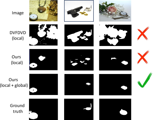
Figure 1: Visualization of co-saliency detections on the pocket watch image group from the CoCA dataset [77]: Row 1: Original image, Row 2: predictions from the DVFDVD model [2] that only mines local patch-level correspondences, Row 3: our predictions with only local (patch) feature correspondence, Row 4: our predictions with both local (patch) and global (region) feature correspondence which produces the best results, Row 5: Ground truth.

The reliance on annotations poses a challenge for the existing fully supervised CoSOD models [16, 72, 77, 14, 68]. To alleviate this burden, certain approaches [40, 25, 26] have focused on unsupervised co-segmentation and co-saliency detection, having several potential real-world applications such as e-commerce, content-based image retrieval, satellite imaging, biomedical imaging, etc. However, these models demonstrate significantly poorer prediction performance compared to their fully supervised counterparts due to their inefficient utilization of unlabeled data at different scales (patch and region levels). For example, Amir et al. [2] only mines local patch-level features such as clustering of ViT patch descriptors for co-segmentation. Also, for some models [65, 5] the performance improvement comes mostly from using heavy off-the-shelf components (such as SAM [34], STEGO [20], DCFM [68], Stable Diffusion [49], etc.) that make their models computation-heavy and hence unfit for real-time applications.

In this paper, we present a lightweight model that leverages feature correspondences at both patch and region levels to improve unsupervised CoSOD performance. We take advantage of the self-supervised features in visual transformers (ViTs) [11, 3] and their self-attention maps [3] to develop a simple yet effective self-supervised CoSOD model that uses both patch and region level feature correspondences, which we call SCoSPARC.

As part of our self-supervised approach, we first train a network to compute cross-attention maps that highlight commonly occurring salient regions via local patch-level feature correspondences across images in the group. We show that these correspondences form strong signals for unsupervised CoSOD. We design this network to optimize two losses: 1) the Co-occurrence loss, which constraints the foreground image regions to have similar feature representations and at the same time, it forces the foreground and background feature representations within each image to be as dissimilar as possible, 2) the Saliency loss, in order to maximize the saliency of the detected regions. While previous approaches [26, 25], have also leveraged similar losses for guiding their model training, we differ from these approaches in two main aspects: 1) we avoid the use of separate off-the-shelf saliency models for training, instead directly leverage the intermediate self-attention maps from our backbone encoder to construct our saliency signal, 2) we construct the foreground and the background feature embeddings directly using the feature descriptors from our backbone encoder (averaged via cross-attention maps) instead of training separate sub-networks to extract the mask embeddings (details in Sec. 3.1). Thus, we effectively leverage the feature encodings from our backbone encoder to construct both of our co-occurrence and saliency signals during training. This helps us maintain our model’s computational efficiency and facilitates fast inference times. Next, we introduce a prediction confidence-based adaptive thresholding method for thresholding the cross-attention maps in order to generate intermediate CoSOD segmentations. While prior works [62, 19] have used adaptive thresholding based on the class confidence in the context of semi-supervised learning, we use adaptive thresholds based on the confidence of the co-saliency predictions, for our task of self-supervised CoSOD. Our model at this stage outperforms the SOTA unsupervised US-CoSOD model [5] by a significant margin (details in Sec. 4). For enforcing region-level feature correspondence, we next identify connected components (corresponding to the detected image regions) in the intermediate segmentation masks and eliminate regions whose feature representations are not similar to the average foreground feature representation obtained from the cross-attention maps in the previous step. Our experiments demonstrate a significant improvement in prediction performance compared to existing works.

In Fig. 1, we show CoSOD predictions from three different methods: 1) the DVFDVD model [2] that only mines local patch-level feature correspondences via clustering of patch descriptors, 2) our predictions with only local (patch-level) feature correspondence, 3) our predictions with both local (patch-level) and more global (region-level) feature correspondences, which produces the best results. Fig. 1 demonstrates the two main contributions of our work: 1) our local patch-level feature correspondence learning network produces better results compared to the existing models e.g. DVFDVD [2] which only clusters the local ViT patch descriptors, 2) using both local (patch-level) and global (region-level) feature correspondences for CoSOD helps improve the results.

We summarize our main contributions as follows:

• We propose a simple yet effective two-stage self-supervised approach for CoSOD that leverages feature correspondences (of self-supervised ViT features) at different scales in an image group.

• We introduce a confidence-based adaptive thresholding approach for the cross-attention maps, outperforming the conventional fixed threshold of 0.5 commonly used in binary segmentation tasks.

• We show that our method outperforms existing unsupervised CoSOD approaches on three benchmarks (e.g., on the CoCA dataset, our model has a 13.7% F-measure gain over the SOTA unsupervised CoSOD model) while also outperforming several popular recent supervised CoSOD methods on these datasets.

2 Related Work

Self-supervised learning: Unlike supervised methods that necessitate human annotation, self-supervised learning involves training networks with automatically generated pseudo-labels that capture characteristics such as image contexts or handcrafted cues in order to accomplish a pretext task (e.g. colorization, rotation prediction, etc.) using unlabeled data [3, 6, 18, 22, 47, 55]. For instance, DINO [3] employs a student-teacher framework where the two networks observe different and randomly transformed input parts, and the student network learns to predict the mean-centered output of the teacher network. Studies based on the DINO ViT features have leveraged these features for tasks such as object discovery [51, 60], semantic segmentation [20, 57], and category discovery [58]. In Masked Auto Encoder [21], patches of the input image are randomly masked, and the pretext task involves learning to reconstruct the missing pixels through auto-encoding. These studies have demonstrated that the representations derived from the self-attention maps of ViTs contain valuable localization information [2, 3, 80]. Our work incorporates both the patch-level ViT feature descriptors and the self-attention maps from DINO to guide our self-supervised network training.

Co-salient object detection: Graphical models are employed to capture pixel relationships within an image collection [27, 30, 31, 32, 63, 73], followed by the extraction of co-salient objects characterized by consistent features. Some approaches leverage supplementary object saliency details to identify salient objects prior to implementing CoSOD [33, 75, 76]. Other methodologies focus on delineating shared attributes among input images [16, 72, 77, 53, 36, 81, 14, 41, 17, 78, 64, 66], complementing semantic information with classification data. Comprehensive insights into CoSOD can be found in related surveys [10, 15, 70].

Unsupervised segmentation: Multiple approaches in unsupervised semantic segmentation leverage self-supervised feature learning methods [29, 42, 56, 9, 60]. Other works tackle unsupervised co-segmentation [28, 40, 25, 2, 4] and CoSOD [71, 26], where Li et al. [40] rank image complexities using saliency maps for unsupervised co-segmentation. Hsu et al. [25] propose an unsupervised co-attention model, and in [26], their unsupervised graphical model jointly handles single-image saliency and object co-occurrence in CoSOD. Recently, Liu et al. [45] introduced a self-supervised CoSOD model using an unsupervised graph clustering algorithm for detection, refining sample affinity with pseudo-labels. Additionally, Xiao et al. [65] presented a zero-shot CoSOD approach that is based on group prompt generation and subsequent co-saliency map generation. Chakraborty et al. [5] proposed unsupervised and semi-supervised CoSOD models using segmentation frequency statistics that leveraged pre-trained models to generate pseudo-labels for training. Although ZS-CSD and US-CoSOD improved unsupervised CoSOD performance, relying on several off-the-shelf components made them computationally heavy. Our method outperforms all of these unsupervised models while maintaining a lightweight design with minimal computational parameters.

The existing unsupervised CoSOD methods suffer from limited performance due to their reliance on handcrafted features and insufficient utilization of feature correspondences at multiple scales. Our study addresses this gap by introducing a self-supervised CoSOD approach that effectively harnesses feature correspondences at different scales to significantly enhance CoSOD performance.

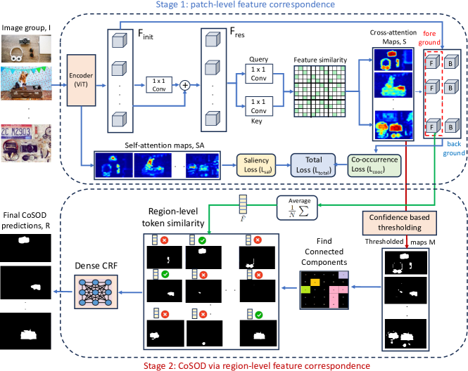
Figure 2: The proposed two-stage self-supervised CoSOD model, SCoSPARC. In the first stage, we train a network that leverages the local ViT feature correspondences across all patches in the images in the group to obtain cross-attention heatmaps, which we further threshold using a confidence-based adaptive threshold to obtain an intermediate binary segmentation map. In the next stage, we refine these segmentations via region-level feature correspondence using the average foreground token obtained from the previous stage, followed by dense CRF-based segmentation refinement.

3 Methodology

Given a group of $N$ images $I=\{I_{1},I_{2},...,I_{N}\}$ containing co-occurring salient objects of a specific class, CoSOD aims to detect them concurrently and output their co-salient object segmentation masks. In self-supervised CoSOD, the goal is to predict the co-salient segmentations $\{\hat{y}_{i}\}_{i=1}^{n}$ without using any labeled data.

Here, we describe our self-supervised CoSOD model, SCoSPARC that employs ViT feature correspondences at both local and region levels to detect the co-salient objects in an image group.

Fig. 2 depicts the pipeline of our SCoSPARC model. In the first stage, we leverage the patch-level (local) ViT feature correspondences across all patches in the images in the group to obtain the cross-attention map. We threshold this map using a confidence-based adaptive threshold to obtain an intermediate binary segmentation map. In the next stage, we refine these intermediate segmentations via region-level feature correspondence using the average foreground token obtained from the previous stage. Finally, we employ dense CRFs [35] to ensure spatial continuity in the predicted segmentations. We will describe each component in detail in the following subsections.

3.1 Stage 1: Patch-level feature correspondences

Previous works on self-supervised learning (SSL) have shown that ViT [11] models (pretrained on ImageNet) using methods such as DINO [3] can provide great features for segmentation tasks due to the explicit semantic information learned via SSL [20, 57]. Motivated by this, we employ the pre-trained ViT trained using DINO as the feature encoder in our pipeline.

We first extract image patch features $\mathbf{x}^{pat}_{n}$ from an image $I_{n}$ in the image group using our ViT Encoder as: $\mathcal{F}_{init}=[\mathbf{x}_{1}^{\textit{pat}},\dots,\mathbf{x}_{N}^{\textit{pat}}]$, where $\mathcal{F}_{init}\in\mathbb{R}^{N\times C\times H\times W}$ ($N$, $C$, $H$, $W$ are the number of images in the group, channel number, height, and width respectively) and $\mathbf{x}^{\textit{pat}}_{n}=Encoder({I_{n}})$.

These features are processed by the residual block to generate residual features $\mathcal{F}_{res}$ as:

$$\centering\mathcal{F}_{res}=\mathcal{F}_{init}+conv^{1\times 1}(\mathcal{F}_{init}),\@add@centering$$ (1)

where $conv^{1\times 1}$ represents for the $1\times 1$ convolution layer and $\mathcal{F}_{res}\in\mathbb{R}^{N\times C\times H\times W}$. This layer when added to the DINO features generate strengthened residual features that better capture the complex relationships in the data. This makes training more efficient and allows faster network convergence.

First, we input the residual features $\mathcal{F}_{res}$ to our network. Next, we employ self-attention by utilizing two $1\times 1$ convolution layers. These layers yield two distinct feature maps, namely the key map $K\in\mathbb{R}^{N\times C\times H\times W}$ and the query map $Q\in\mathbb{R}^{N\times C\times H\times W}$. After reshaping both $K$ and $Q$ to shape $\mathbb{R}^{NHW\times C}$, we compute the feature similarity matrix $S$ as:

$$\centering S=\frac{1}{\sqrt{d}}KQ^{\top},\@add@centering$$ (2)

where $S\in\mathbb{R}^{NHW\times NHW}$, $d$ = embedding dimension, and $\top$ denotes the transpose operation. Each row of $S$ represents feature token similarities between a patch (corresponding to the row) and all other patches of the $N$ input images. The feature similarity matrix S is then reshaped to shape $S\in\mathbb{R}^{N\times HW\times NHW}$. Next, we construct a 1D-map $S^{\prime}_{n}\in\mathbb{R}^{HW}$ from the matrix $S$ for each image $I_{n}$ in the group by computing the row-wise mean of $S$ as: $S^{\prime}_{n}(p)=\frac{1}{NHW}\sum_{p^{\prime}=1}^{NHW}S_{p^{\prime}}$, where $p$ denotes a patch in $S_{n}$ and $p^{\prime}$ is the corresponding index of patch $p$ (of $S^{\prime}_{n}$) in the matrix S. Each 1D-map $S^{\prime}_{n}\in\mathbb{R}^{HW}$ is next reshaped to a 2D-map $S_{n}\in\mathbb{R}^{H\times W}$. Maps $S_{n}$ are then separately normalized using min-max normalization.

Although the pixel values of ground truth maps are either 0 or 1, those of the predicted feature similarity maps $S$ contain intermediate intensity values (between 0 and 1), which indicate uncertainty and noise in the predictions. To deal with these uncertain values, we employed a modified version of the Sigmoid function  [43] with a parameter $k$ that controls the steepness of Sigmoid and encourages the map values of $S_{n}$ to be close to either 0 or 1. $s_{th}$ is the confidence threshold. We represent the intermediate cross-attention maps $\mathcal{M}$ as:

$$\mathcal{M}_{n}=\frac{1}{1+e^{-k(S_{n}-s_{th})}},$$ (3)

Due to the nature of the task (co-salient object detection), we expect the detected co-salient regions across all images in the group to share similar feature representations in terms of object semantics and at the same time have a high saliency at an individual level. Therefore, we use a combination of two different loss terms to train our network in a self-supervised manner: (1) the co-occurrence loss $\mathcal{L}_{cooc}$ that measures the quality of the detected co-occurrent foreground regions between an image pair, and (2) the saliency loss $\mathcal{L}_{sal}$ that estimates the total saliency of the detected regions for an image. We define the co-occurrence loss $\mathcal{L}_{cooc}$ between images $I_{n}$ and $I_{m}$ as:

$$\mathcal{L}_{cooc}=\sum_{n=1}^{N}\sum_{m=n}^{N}\frac{\exp({-d^{+}_{nm}})}{\exp({-d^{+}_{nm}})+\exp({-d^{-}_{nm}})}$$ (4)

$$d^{+}_{nm}=1-\cos({f(\mathcal{M}^{f}_{n},\mathbf{x}^{pat}),f(\mathcal{M}^{f}_{m},\mathbf{x}^{pat})})$$ (5)

$$d^{-}_{nm}=1-(\cos({f(\mathcal{M}^{f}_{n},\mathbf{x}^{pat}),f(\mathcal{M}^{b}_{n},\mathbf{x}^{pat})})+\cos({f(\mathcal{M}^{f}_{m},\mathbf{x}^{pat}),f(\mathcal{M}^{b}_{m},\mathbf{x}^{pat})}))$$ (6)

where $f(m,\mathbf{x}^{pat})=\frac{1}{n_{p}}\sum_{i=1}^{n_{p}}m_{i}\otimes\mathbf{x}^{pat}_{i}$ denotes the average ViT feature embedding corresponding to the mask $m$ and the patch descriptor $\mathbf{x}^{pat}$ ($n_{p}$ = total number of patches in $m$). $\mathcal{M}_{i}^{f}=\mathcal{M}_{i}$ is the foreground mask (which is the cross-attention map) and $\mathcal{M}_{i}^{b}=1-\mathcal{M}_{i}$ is the background mask corresponding to the image $I_{i}$. Here $cos$ denotes the cosine-similarity function.

Trained with the self-distillation loss [23], the attention maps associated with the class token from the last layer of DINO [3] have been shown to highlight salient foreground regions [3, 61, 67]. Their findings revealed that the attention heads of this model focus on significant foreground regions within an image. Motivated by this observation, we consider the averaged attention map (across all attention heads) from DINO as the foreground object segmentation. First, we average the self-attention maps from the $n_{h}$ DINO attention heads to obtain the averaged self-attention map $SA_{i}$ for an image $I_{i}$ as: $SA_{i}=\frac{1}{n_{h}}\sum_{j=1}^{n_{h}}AM_{i}^{j}$, where $AM_{i}^{j}$ is the attention map from the DINO attention head $j$ for the image $I_{i}$. Map $SA_{i}$ is normalized by min-max normalization. Subsequently, the saliency loss $\mathcal{L}_{sal}$ is computed as:

$$\mathcal{L}_{sal}=1-\frac{1}{N}\sum_{n=1}^{N}\mathcal{M}_{n}\otimes SA_{n},$$ (7)

The network is self-supervised using a combination of the co-occurrence and the saliency loss terms as:

$$\mathcal{L}_{total}=\mathcal{L}_{cooc}+\lambda_{sal}\mathcal{L}_{sal}$$ (8)

where $\lambda_{sal}$ is the weight accounting for the saliency factor. Minimizing the saliency loss maximizes the average saliency of the detections. For co-occurring non-salient objects, the saliency loss is low and training/inference proceeds via the co-occurrence loss.

Confidence based adaptive thresholding:

While we enforce the map intensity values to be close to 0 or 1 (as explained in the previous paragraph), we require an additional thresholding step to obtain binary segmentation masks for each image. We observed that a more confident attention map requires a lower threshold and conversely, a less confident map requires a higher threshold in order to accurately predict a binary segmentation map of the co-salient regions. Consequently, the default threshold value of 0.5, used by the existing segmentation models (via the argmax operator) does not produce the best performance. Informed by this observation, we adaptively threshold the predicted cross-attention map $\mathcal{M}_{n}$ based on the confidence of the detected regions. To this end, we first compute the average confidence of the detected regions in the map $\mathcal{M}_{n}$ and then select the threshold $th$ as:

$$c_{M}=\frac{1}{n_{conf}}\sum_{p:p\geq\overline{\mathcal{M}}}\mathcal{M}_{p}$$ (9)

$$b_{M}=1-c_{M}$$ (10)

$$th=th_{0}+\alpha_{c}(b_{M}-\overline{b_{M}})$$ (11)

$$G_{n}=\begin{cases}1&\text{if }\mathcal{M}_{n}\geq th\\ 0&\text{if }\mathcal{M}_{n}<th\end{cases}$$ (12)

where $n_{conf}$ is the number of confident map pixels i.e. pixels with an intensity greater than the average intensity value $\overline{\mathcal{M}}$. $c_{M}$ denotes the average per-pixel confidence of the predicted map M for an image $I_{n}$ in the image group. $b_{M}$ is the inverse of the average confidence value of map M and $\overline{b_{M}}$ denotes the average value of $b_{M}$ over the training dataset. We set the adaptive threshold $th$ as $(b_{M}-\overline{b_{M}})$ offset by an initial threshold $th_{0}$. Thus, we threshold each map $\mathcal{M}_{n}$ to obtain the segmentation mask $G_{n}$ for each image ${I_{n}}$ in the image group I. See supplementary for more details.

Algorithm 1 Stage 2: Region-level mask refinement

0:  Image group $I=\{I_{n}\}_{i=1}^{N}$, intermediate segmentation mask $G=\{G_{n}\}_{i=1}^{N}$

0:  Refined segmentation mask $R=\{R_{n}\}_{i=1}^{N}$

1:  Obtain the average token embedding $F_{G}$ corresponding to the masks $G$ across all images as:$F_{G}=\frac{1}{N}\sum_{i=1}^{N}\frac{1}{Ar(G_{i})}\sum x_{i}^{patch}\otimes G_{i}$, $Ar(A)=$ area of region A.

2:  for $i=1$ to $n$ do

3:     Apply connected component labeling on mask $G_{i}$ to generate $L_{i}$ masks for each component.

4:     Map $R_{i}\leftarrow$ all-zero map (same size as $G_{i}$) 

5:     for $j=1$ to $L_{i}$ do

6:        Obtain the feature embedding $F_{G_{ij}}$ corresponding to the mask region $G_{ij}$ by averaging the patch embeddings as: $F_{G_{ij}}=\frac{1}{Ar(G_{ij})}\sum x_{i}^{patch}\otimes G_{ij}$.

7:        Compute the similarity between the token embeddings $F_{G}$ and $F_{G_{ij}}$ as: $d=\cos(F_{G},F_{G_{ij}})$, $\cos$ is the cosine distance. if $d_{f}\geq d_{f}^{th}$ then:   $R_{i}=R_{i}\cup G_{ij}$ end if

8:     end for

9:  end for

10:  return  Refined masks, $R=\{R_{n}\}_{i=1}^{N}$

3.2 Stage 2: Region-level feature correspondences

The regions highlighted in the binary segmentation maps $S$ obtained from stage 1 do not always belong to the co-salient object in the image group as shown in Sec. 4. This is because the patch-level feature correspondences fail to capture the region-level semantics of the co-occurring object. To solve this problem, we eliminate regions whose feature are dissimilar with the average consensus token representation i.e. the averaged token embeddings of the detected common foreground regions.

Our mask refinement algorithm is outlined in Algorithm 1. First we obtain the average token embedding $F_{S}$ corresponding to the masks $S$ across all images by averaging the ViT patch embeddings. Next, we implement connected component labeling on the masks S in order to get sub-masks $L$ corresponding to the disconnected regions in these masks. For each sub-mask in each image, we compute the feature token similarity of the sub-mask with respect to the averaged token embedding $F_{S}$ and only retain sub-masks beyond a threshold similarity score $d_{f}^{th}$.

Postprocessing using denseCRFs:

Finally, we improve the co-salient segmentations $R_{n}$ obtained in the previous step by enforcing spatial coherence and preserving object boundaries in the predictions using denseCRFs following previous work [24, 38] for every image $I_{n}$ in the group.

4 Experimental Results

4.1 Setup

Datasets and evaluation metrics: For training our self-supervised SCoSPARC model, we used images from COCO9213 [59], a subset of the COCO dataset [44] containing 9,213 images selected from 65 groups, and from the DUTS class dataset [77] that contains 8,250 images in total distributed across 291 groups. We evaluate our methods on three popular CoSOD benchmarks: CoCA [77], Cosal2015 [71], and CoSOD3k [15]. CoCA and CoSOD3k are challenging real-world co-saliency evaluation datasets, containing multiple co-salient objects in some images, large appearance and scale variations, and complex backgrounds. Cosal2015 is a widely used dataset for CoSOD evaluation.

Our evaluation metrics include the Mean Absolute Error (MAE$\downarrow$) [8], maximum F-measure ($F_{\beta}^{max}\uparrow$) [1], maximum E-measure ($E_{\phi}^{max}\uparrow$) [13], and S-measure ($S_{\alpha}\uparrow$) [12].

Implementation details: We use the ViT-B model (with patch size = 8 and patch descriptor dimension $d$ = 768) trained using DINO as our backbone feature extractor. For training, we set the sample size as the minimum of 24 or the total group size. At inference, all samples (resized to $224\times 224$) in the group are input at once. We used the Adam optimizer to train our stage 1 network for 80 epochs. The total training time is around 10 hours. The inference speed of the model is 20 FPS (without dense CRF) and 4 FPS (with dense CRF). All experiments are run on an NVIDIA Quadro RTX 8000 GPU. In Eq. 3, we empirically set the parameter $k$ to 6.66 and the threshold parameter $s_{th}$ to 0.65. In Eq. 7 we set $\lambda_{sal}$ to 0.3. Increasing this value produced segmentations highlighting salient regions but not co-occurring. Decreasing this value highlighted commonly occurring background regions e.g. sky, roads, etc. as being co-salient. We empirically set the embedding similarity threshold as $d_{f}^{th}=0.75$ in Algorithm 1. In Eq. 11 we empirically set $\alpha_{c}$ to 1 and $th_{0}$ to 0.5 (a widely used segmentation threshold). More details in the supplementary.

Table 1: Quantitative ablation studies of the proposed components in our model.

	Component					CoCA [77]				CoSal2015 [71]				CoSOD3k [15]
ID	Co-oc.	Sal.	CAT	RFC	D-CRF	$MAE\downarrow$	$F_{\beta}^{max}\uparrow$	$E_{\phi}^{max}\uparrow$	$S_{\alpha}\uparrow$	$MAE\downarrow$	$F_{\beta}^{max}\uparrow$	$E_{\phi}^{max}\uparrow$	$S_{\alpha}\uparrow$	$MAE\downarrow$	$F_{\beta}^{max}\uparrow$	$E_{\phi}^{max}\uparrow$	$S_{\alpha}\uparrow$
1	✓					0.105	0.565	0.756	0.678	0.075	0.851	0.892	0.823	0.077	0.801	0.868	0.793
2	✓	✓				0.105	0.564	0.754	0.678	0.072	0.853	0.895	0.830	0.075	0.810	0.869	0.798
3	✓	✓	✓			0.105	0.567	0.756	0.679	0.069	0.840	0.893	0.832	0.069	0.802	0.878	0.808
4	✓	✓	✓	✓		0.095	0.601	0.776	0.701	0.067	0.851	0.898	0.838	0.067	0.814	0.882	0.812
5	✓	✓	✓	✓	✓	0.092	0.614	0.782	0.711	0.062	0.869	0.905	0.851	0.064	0.827	0.889	0.820

Table 2: Comparison of our model with other state-of-the-art models on 3 benchmarks. We achieve state-of-the-art performance for unsupervised CoSOD (upper block). Interestingly, our self-supervised SCoSPARC model outperforms recent supervised CoSOD methods (e.g. DCFM, CoRP, UFO, etc.) while being comparable to the SOTA (lower block).

	CoCA [77]				Cosal2015 [71]				CoSOD3k [15]
Method	MAE$\downarrow$	$F_{\beta}^{max}\uparrow$	$E_{\phi}^{max}\uparrow$	$S_{\alpha}\uparrow$	MAE$\downarrow$	$F_{\beta}^{max}\uparrow$	$E_{\phi}^{max}\uparrow$	$S_{\alpha}\uparrow$	MAE$\downarrow$	$F_{\beta}^{max}\uparrow$	$E_{\phi}^{max}\uparrow$	$S_{\alpha}\uparrow$
UCCDGO [26] (ECCV 2018)	-	-	-	-	-	0.758	-	0.751	-	-	-	-
TokenCut [60] (CVPR 2022)	0.167	0.467	0.704	0.627	0.139	0.805	0.857	0.793	0.151	0.720	0.811	0.744
DVFDVD [2] (ECCVW 2022)	0.223	0.422	0.592	0.581	0.092	0.777	0.842	0.809	0.104	0.722	0.819	0.773
SegSwap [50] (CVPRW 2022)	0.165	0.422	0.666	0.567	0.178	0.618	0.720	0.632	0.177	0.560	0.705	0.608
SAM CSD [45] (Elsevier CEE 2023)	-	-	-	-	0.092	0.782	0.847	0.782	0.108	0.703	0.810	0.723
Zero-Shot CoSOD [65] (ArXiV 2023)	0.115	0.549	-	0.667	0.101	0.799	-	0.785	0.117	0.691	-	0.723
US-CoSOD [5] (WACV 2024)	0.116	0.546	0.743	0.672	0.070	0.845	0.886	0.840	0.076	0.779	0.861	0.801
Group TokenCut	0.106	0.596	0.781	0.701	0.091	0.823	0.867	0.815	0.097	0.757	0.833	0.776
SCoSPARC (ours)	0.092	0.614	0.782	0.711	0.062	0.869	0.905	0.851	0.064	0.827	0.889	0.823
GCAGC [73] (CVPR 2020)	0.111	0.523	0.754	0.669	0.085	0.813	0.866	0.817	0.100	0.740	0.816	0.785
GICD [77] (ECCV 2020)	0.126	0.513	0.715	0.658	0.071	0.844	0.887	0.844	0.079	0.770	0.848	0.797
CoEGNet [14] (TPAMI 2021)	0.106	0.493	0.717	0.612	0.077	0.832	0.882	0.836	0.092	0.736	0.825	0.762
GCoNet [16] (CVPR 2021)	0.105	0.544	0.760	0.673	0.068	0.847	0.887	0.845	0.071	0.777	0.860	0.802
CSG [74] (TMM 2022)	0.106	0.532	0.739	0.671	0.062	0.841	0.895	0.845	0.087	0.753	0.842	0.788
DCFM [68] (CVPR 2022)	0.085	0.598	0.783	0.710	0.067	0.856	0.892	0.838	0.067	0.805	0.874	0.810
CoRP [81] (TPAMI 2023)	-	0.551	-	0.686	-	0.885	-	0.875	-	0.798	-	0.820
UFO [53] (TMM 2023)	0.095	0.571	0.782	0.697	0.064	0.865	0.906	0.860	0.073	0.797	0.874	0.819
MCCL [79] (AAAI 2023)	0.103	0.590	0.796	0.714	0.051	0.891	0.927	0.890	0.061	0.837	0.903	0.858
GEM [64] (CVPR 2023)	0.095	0.599	0.808	0.726	0.053	0.882	0.933	0.885	0.061	0.829	0.911	0.853
DMT [41] (CVPR 2023)	0.108	0.619	0.800	0.725	0.045	0.905	0.936	0.897	0.063	0.835	0.895	0.851
GCoNet+ [78] (TPAMI 2023)	0.081	0.637	0.814	0.738	0.056	0.891	0.924	0.881	0.062	0.834	0.901	0.843

Table 3: Comparison of our model with the SOTA supervised CoSOD model, GCoNet+ using different amounts of labeled data for training.

		CoCA [77]				Cosal2015  [71]				CoSOD3k  [15]
Method	Label	MAE$\downarrow$	$F_{\beta}^{max}\uparrow$	$E_{\phi}^{max}\uparrow$	$S_{\alpha}\uparrow$	MAE$\downarrow$	$F_{\beta}^{max}\uparrow$	$E_{\phi}^{max}\uparrow$	$S_{\alpha}\uparrow$	MAE$\downarrow$	$F_{\beta}^{max}\uparrow$	$E_{\phi}^{max}\uparrow$	$S_{\alpha}\uparrow$
GCoNet+ [78]	50%	0.133	0.534	0.753	0.661	0.074	0.842	0.889	0.842	0.079	0.783	0.865	0.808
GCoNet+ [78]	75%	0.113	0.547	0.759	0.682	0.066	0.863	0.902	0.860	0.071	0.804	0.876	0.823
SCoSPARC (ours)	0%	0.092	0.614	0.782	0.711	0.062	0.869	0.905	0.851	0.064	0.827	0.889	0.823

4.2 Quantitative evaluation

Ablation Studies:

In Tab. 1 we ablate the performance of our model using the different components, namely, the co-occurrence loss (Co-oc.), saliency loss (Sal.), confidence based adaptive thresholding (CAT), region-level feature correspondence (RFC), and dense CRF (d-CRF). We observe that the saliency loss is useful for the Cosal2015 and the CoSOD3k test datasets. This could be attributed to the fact that CoCA focuses more on segmenting the common objects in complex contexts, while Cosal2015 plays a more critical role in testing the ability of models to detect salient objects, as highlighted by [78]. Nevertheless, we use the saliency loss in order to have a more generalized model. The confidence based adaptive thresholding (CAT) step in row 3 leads to an improved performance across most metrics compared to using a fixed threshold of 0.5 in rows 1 and 2. Our region-level feature correspondence leads to a consistent improvement in performance by all metrics and across all the three test datasets. Finally, the dense CRF based post processing step leads to a consistent improvement in performance across all metrics and datasets. While dense CRFs improved segmentation performance of our model, even without this we outperform the SOTA unsupervised US-CoSOD (Tab. 2) by a significant margin (see Tab. 1).

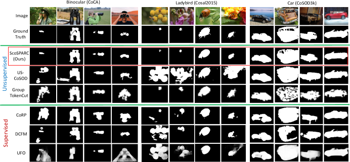
Figure 3: Qualitative comparison of the performance of different baselines with our SCoSPARC on three image groups, each selected from the CoCA, Cosal2015, and CoSOD3k datasets. Our model produces the most accurate segmentations.

Comparison with the state-of-the-art (SOTA) methods:

In Tab. 2 we compare the performance of our model with the existing unsupervised CoSOD models (upper block) as well as supervised CoSOD models (lower block).

In the upper block in Tab. 2, we see that our SCoSPARC outperforms all existing unsupervised CoSOD models. We introduce a baseline, Group TokenCut, a modified version of the popular TokenCut [60] model used for single-image foreground segmentation. In Group TokenCut, we calculate the second smallest eigenvector of a graph (indicating the likelihood of a token belonging to a foreground object) constructed across all patch-level tokens in the image group (from all images), differing from TokenCut’s second smallest eigenvector computation based on a single image. We outperform the SOTA for unsupervised CoSOD i.e. the US-CoSOD model [5], by a significant margin (we achieve a 13.7% gain in the F-measure metric over US-CoSOD on the CoCA dataset).

Interestingly, in the lower block in Tab. 2, we see that SCoSPARC outperforms several SOTA fully supervised CoSOD models such as DCFM [68], CoRP [81], UFO [53], etc. Also, we outperform the recent MCCL [79] and GEM [64] models on the CoCA dataset in terms of $F^{max}_{\beta}$-measure and MAE.

In Tab. 3 we quantitatively compare the performance of our SCoSPARC model with GCoNet+ [78] when limited data is available for training. Specifically, we evaluated GCoNet+ using 50% and 75% training labels i.e. we randomly selected a fraction of images from each image group in the training dataset as the labeled set. We find that GCoNet+ has worse performance compared to SCoSPARC using 50% labels across all metrics, and in the majority of metrics using 75% labels. We attribute the poor performance of GCoNet+ to the fact that this model overfits to the training data when limited data is available for training. Other supervised models such as CoRP [81], DCFM [68], and UFO [53] also perform poorly compared to our model due to the same reason. Our self-supervised model, on the other hand, better leverages the patch and region feature correspondences within the images without relying on labeled training data (thus avoiding overfitting), which improves prediction performance.

In Tab. 4 we compare the inference speeds of our SCoSPARC (with and without dense CRFs) with other unsupervised CoSOD baselines, namely SegSwap [50], DVFDVD [2], and Group TokenCut. SCoSPARC without the dense CRF step achieves the highest inference speed, in terms of the frames-per-second (FPS). Tab. 1 and Tab. 2 show that our model outperforms all SOTA unsupervised CoSOD models and remains competitive with the recent supervised CoSOD models even without the dense-CRF post processing step.

Table 4: Comparison of the inference speeds of SCoSPARC (with and without dense CRFs) with other unsupervised CoSOD baselines.

Method	Inference Speed (FPS)
SegSwap [50] (CVPRW 2022)	0.50
DVFDVD [2] (ECCVW 2022)	0.23
Group TokenCut	0.05
SCoSPARC (ours)	4.1
SCoSPARC w/o d-CRF (ours)	20.5

4.3 Qualitative evaluation

In Fig. 5 we qualitatively compare the CoSOD predictions from our self-supervised SCoSPARC model with different baselines on three image groups, each from the CoCA, CoSOD3k, and Cosal2015 datasets. We compare our model with the unsupervised models US-CoSOD [5] and Group TokenCut, and with the supervised models CoRP [64], DCFM [68], and UFO [53]. We observe that our SCoSPARC generates more accurate segmentations compared to other baselines. The unsupervised US-CoSOD [5] and the Group TokenCut models produce masks with several undesirable image regions (e.g. the non-co-occurring foregrounds) that are responsible for their poor performances. While the supervised CoRP and the DCFM models generate reasonable segmentations in most cases, they fail to accurately detect the small objects for certain instances. For example, for the Ladybird group from Cosal2015, in columns 1 and 2, most methods including CoRP and DCFM produce several undesirable image regions (in the flowers) while failing to accurately segment the small sized ladybird. Our model does not suffer from such drawbacks. UFO [53] produces diffuse segmentation maps, often leading to noisy predictions. In columns 2 and 3 of the car group, we see failure cases where all models including ours erroneously detect background regions inter-leaving the windows as being salient. More results in supplementary.

In Fig. 4 we visualize the intermediate maps from our SCoSPARC model, namely the self-attention map, $SA$ from the DINO ViT backbone in column 2, the cross-attention map $S$ (from stage 1) in column 3, the thresholded segmentation map $G$ (following confidence based adaptive threshold) in column 4, the final segmentation $R$ (from stage 2) in column 5, and the ground truth in column 6, for the handbag image group from the CoCA dataset. In column 4 in Fig. 4, we highlight the regions eliminated using our region-based feature correspondence step (in stage 2) using dashed yellow boxes. We observe that this step only retains the image regions that correspond well with the semantic information of the co-occurring object (handbag in this case) while eliminating undesirable image regions initially detected using local feature correspondence in stage 1. More results in the supplementary.

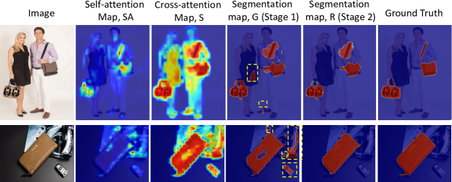
Figure 4: Visualizations of intermediate self-attention maps, cross-attention maps, and segmentation maps for two instances from the handbag category from CoCA. The yellow boxes highlight the regions eliminated using stage 2 of our SCoSPARC model.

5 Conclusion

We presented a novel self-supervised approach for CoSOD based on mining feature correspondences at multiple scales within a group of images. Our model first finds local patch-level correspondences via a network trained to maximize co-occurrence and saliency of the detected regions in a self-supervised manner. We further employ a more global region-level correspondence to eliminate detected regions that do not align well with the consensus feature representation across the entire image group, which yields improved predictions. The proposed model outperforms all existing unsupervised methods and several popular supervised models for co-salient object detection. As future work, we would like to investigate the use of stable diffusion models (which has shown promising results for segmentation tasks) for self-supervised CoSOD using pseudo-labels from the proposed method.

In this supplementary document, we provide details about our experiments and present more results from our study. The document is organized into the following sections:

1. Section  6: Additional quantitative results

2. Section  7: Additional qualitative results

3. Section  8: Additional implementation details

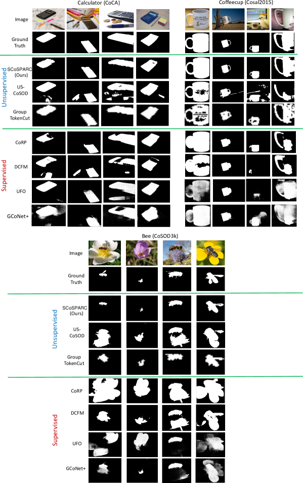
Figure 5: Additional qualitative comparison of the performance of different baselines with our self-supervised CoSOD model on three image groups, each selected from the CoCA, Cosal2015, and CoSOD3k datasets. Our model produces the most accurate segmentations.

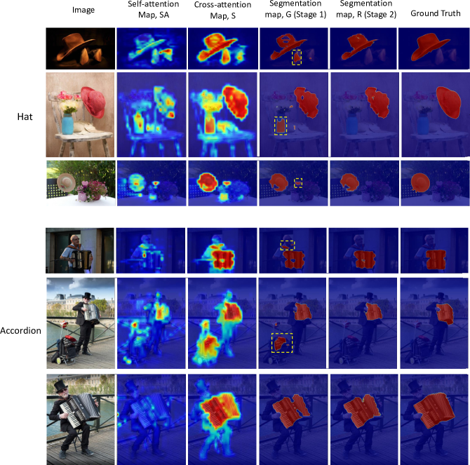
Figure 6: Additional visualizations of the intermediate self-attention maps, cross-attention maps and segmentation maps for two instances from the handbag category from the CoCA dataset. The yellow boxes highlight the regions eliminated using the stage 2 of our SCoSPARC model.

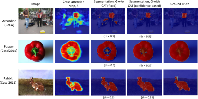
Figure 7: Visualizations of the segmentation map, G (from stage 1) with and without our confidence-based adaptive thresholding (CAT) component. Our model with CAT produces more accurate segmentation predictions.

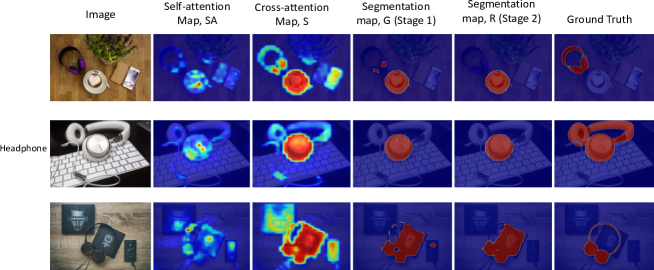
Figure 8: Some failure cases of predictions on the headphone image group from CoCA.

6 Additional quantitative results

6.1 Performance using different training datasets

In Tab. 5 we compare the segmentation performance of our stage 1 self-supervised network when trained on the two datasets, namely COCO9213 [59] and DUTS-Class [77]. We observe that training on a combination of the two datasets provides the best performance across all metrics and test datasets.

Table 5: Comparison of the segmentation performance of our stage 1 self-supervised network when trained on the two datasets, namely COCO9213 and DUTS Class. Training on a combination of the two datasets provides the best performance.

	CoCA [77]				Cosal2015 [71]				CoSOD3k [15]
Method	MAE$\downarrow$	$F_{\beta}^{max}\uparrow$	$E_{\phi}^{max}\uparrow$	$S_{\alpha}\uparrow$	MAE$\downarrow$	$F_{\beta}^{max}\uparrow$	$E_{\phi}^{max}\uparrow$	$S_{\alpha}\uparrow$	MAE$\downarrow$	$F_{\beta}^{max}\uparrow$	$E_{\phi}^{max}\uparrow$	$S_{\alpha}\uparrow$
COCO9213 [59]	0.115	0.532	0.737	0.659	0.072	0.824	0.887	0.824	0.074	0.781	0.866	0.800
DUTS-Class [77]	0.105	0.555	0.760	0.674	0.071	0.837	0.890	0.828	0.070	0.801	0.878	0.805
COCO9213 [59] + DUTS-Class [77]	0.104	0.567	0.756	0.679	0.069	0.844	0.894	0.832	0.069	0.806	0.878	0.808

6.2 Performance using other encoder backbones

In Tab. 6, we show the effect of using different encoder backbones on the segmentation performance of our stage 1 self-supervised network. The ViT-Base encoder (embedding size = 768) with patch size = 8 provides the best performance, which we use in our final model. The convolution-based VGG-16 backbone [52] has a significantly worse performance compared to the other ViT-based backbones. For ViT encoders, we observe that increasing the patch size from 8 to 16 (or reducing the prediction resolution) leads to a significant drop in performance e.g. the F-measures on CoCA, Cosal2015 and CoSOD3k fall from 0.567, 0.844, 0.806 to 0.511, 0.760, and 0.664 respectively. Also, reducing the encoder’s representation ability using a reduced embedding size (using the ViT-Small backbone) while keeping the patch size same leads to a drop in performance e.g. the F-measures on CoCA, Cosal2015 and CoSOD3k fall from 0.567, 0.844, 0.806 to 0.560, 0.830, and 0.752 respectively.

Table 6: The effect of using different encoder backbones on the segmentation performance of our stage 1 self-supervised network. The ViT-Base encoder with patch size = 8 provides the best performance.

	CoCA [77]						Cosal2015 [71]				CoSOD3k [15]
Encoder	Patch size	Embedding size	MAE$\downarrow$	$F_{\beta}^{max}\uparrow$	$E_{\phi}^{max}\uparrow$	$S_{\alpha}\uparrow$	MAE$\downarrow$	$F_{\beta}^{max}\uparrow$	$E_{\phi}^{max}\uparrow$	$S_{\alpha}\uparrow$	MAE$\downarrow$	$F_{\beta}^{max}\uparrow$	$E_{\phi}^{max}\uparrow$	$S_{\alpha}\uparrow$
VGG-16	16	512	0.115	0.356	0.632	0.518	0.205	0.475	0.553	0.505	0.173	0.468	0.572	0.517
ViT-Base	16	768	0.116	0.511	0.743	0.640	0.092	0.760	0.863	0.785	0.119	0.664	0.792	0.724
ViT-Small	8	384	0.105	0.559	0.755	0.667	0.091	0.810	0.851	0.789	0.081	0.779	0.852	0.778
ViT-Base	8	768	0.104	0.567	0.756	0.679	0.069	0.844	0.894	0.832	0.069	0.806	0.878	0.808

7 Additional qualitative results

7.1 Comparison of CoSOD predictions

In Fig. 5 we qualitatively compare the CoSOD predictions from our SCoSPARC model with two unsupervised CoSOD models US-CoSOD [5] and Group TokenCut and with four recent supervised models CoRP [64], DCFM [68], UFO [53] and GCoNet+ [78].

For the Calculator class, we observe that the US-CoSOD model produces undesirable image regions as CoSOD detections. Our Group TokenCut baseline produces reasonably good detections in this case, although there are edge artifacts. The supervised models such as CoRP and DCFM produce incomplete segmentations in several instances (columns 1, 3 and 4). The DCFM model also segments undesirable image regions e.g. the paper in column 1 and the pen in column 2. The UFO model inaccurately segments the pen as being co-salient in column 3. Finally, the GCoNet+ model, although being SOTA in supervised CoSOD, produces noisy predictions for this image group. Our model produces the best results in general.

For the Coffecup class, in column 1 we observe that all models except SCoSPARC produce either incomplete segmentations (e.g. not detecting the textual regions on the cup) or inaccurately segment undesirable regions (e.g. CoRP segments the background region between the cup handle). Similarly, in column 2, most baseline models inaccurately segment the background region between the cup handle. Also, in the third column, we see that our model produces the best results while other baselines produce inaccurate segmentations. In column 4, Group TokenCut produces comparable results to our predictions, while other models produce noisy segmentations.

For the Bee class, most models except Group TokenCut inaccurately detect flower parts as being co-salient. While Group TokenCut produces reasonable segmentations in this case, the predictions of our SCoSPARC are more refined.

7.2 Visualizations of intermediate maps

In Fig. 6 we show additional visualizations of the intermediate self-attention maps, cross-attention maps and segmentation maps for two image groups, Hat and Accordion (three instances each) from the CoCA dataset. The yellow boxes highlight the regions eliminated using the stage 2 of our SCoSPARC model. We observe that undesirable image regions (i.e. non-co-salient regions highlighted by the yellow boxes) are eliminated in stage 2 segmentation predictions, $\mathcal{R}$ from our model using our region-level feature correspondence step (RFC).

7.3 Visualizations of confidence-based adaptive thresholding results

In Fig. 7, we visualize the segmentation maps, G (from stage 1) with and without our confidence-based adaptive thresholding (CAT) component. We see that our model with CAT produces more accurate segmentation predictions. In row 1 of Fig. 7 (for an instance from the Accordion category), we see that the CAT step eliminates undesirable image regions using a higher threshold of 0.56 (determined via prediction confidence) compared to the segmentation obtained using a fixed threshold of 0.5 (widely used in segmentation tasks). On the other hand, for the categories Pepper and Rabbit, we see that lower threshold values of 0.37 and 0.35 produces better segmentations respectively, compared to the fixed 0.5 threshold. The different threshold values predicted by our CAT step are based on the different average confidence intensities of the confident regions in the cross-attention map, $\mathcal{S}$ for the three cases. For example, the per-pixel confidence value (within the confident regions) of the map S for the Accordion category (row 1) is lesser than the per-pixel confidence values for the Pepper and Rabbit categories, which leads the algorithm to predict a higher threshold for Accordion compared to the other two categories in rows 2 and 3. This results in improved segmentations.

7.4 Failure cases

In Fig. 8 we show some failure cases of our SCoSPARC model on the Headphone image group from the CoCA dataset. In row 1 the model misses the headphone and instead highlights the cup and plate as the co-salient objects. In row 2 only one side of the headphone object has been accurately segmented while the model fails to detect the other half including the headband. We observe that a lower threshold on the cross-attention map, S could have produced an improved segmentation (highlighting all parts of the headphone), which our model fails to predict. In row 3, our model predicts certain undesirable regions as being co-salient along with the headphone.

8 Additional implementation details

8.1 Training details

We use the ViT-Base model (with patch size = 8 and patch descriptor dimension = 768) trained using DINO as our backbone feature extractor. We freeze the weights of this backbone for all of our experiments. See Tab. 6 for more ablations on the encoder choice. For training, we set the sample size as the minimum of 24 or the total group size. We input images with size $224\times 224$. Using the ViT-Base model with patch size = 8 produces co-attention maps with size ($\frac{224}{8},\frac{224}{8}$) = $28\times 28$.

We used the PyTorch deep learning library and the Adam optimizer to train our stage 1 network. We set the learning rate to $10^{-4}$ and the weight decay parameter to $10^{-4}$. The total training time for SCoSPARC is around 10 hours for 80 epochs. All experiments are run on an NVIDIA Quadro RTX 8000 GPU.

8.2 Inference details

At inference, all samples (resized to $224\times 224$) in the group are input at once. The inference speed of the model is 20 FPS (without dense CRF) and 4 FPS (with dense CRF).

For the dense CRF [35] post-processing step , we generated the unary operator directly from the binary segmentation map, $\mathcal{R}$ from stage 2. We set the smoothness kernel parameter $\theta_{\gamma}=10$ and the appearance kernel parameters, $\theta_{\alpha}$ and $\theta_{\beta}$ to $10$ and $3$ respectively.

References

- [1] Achanta, R., Hemami, S., Estrada, F., Susstrunk, S.: Frequency-tuned salient region detection. In: 2009 IEEE conference on computer vision and pattern recognition. pp. 1597–1604. IEEE (2009)
- [2] Amir, S., Gandelsman, Y., Bagon, S., Dekel, T.: Deep vit features as dense visual descriptors. ECCVW What is Motion For? (2022)
- [3] Caron, M., Touvron, H., Misra, I., Jégou, H., Mairal, J., Bojanowski, P., Joulin, A.: Emerging properties in self-supervised vision transformers. In: Proceedings of the IEEE/CVF International Conference on Computer Vision. pp. 9650–9660 (2021)
- [4] Chakraborty, S., Mitra, P.: A site entropy rate and degree centrality based algorithm for image co-segmentation. Journal of Visual Communication and Image Representation 33, 20–30 (2015)
- [5] Chakraborty, S., Naha, S., Bastan, M., C., A.K.K., Samaras, D.: Unsupervised and semi-supervised co-salient object detection via segmentation frequency statistics. In: Proceedings of the IEEE/CVF Winter Conference on Applications of Computer Vision (WACV). pp. 332–342 (January 2024)
- [6] Chen, T., Kornblith, S., Norouzi, M., Hinton, G.: A simple framework for contrastive learning of visual representations. In: International conference on machine learning. pp. 1597–1607. PMLR (2020)
- [7] Chen, Z., Xu, Q., Cong, R., Huang, Q.: Global context-aware progressive aggregation network for salient object detection. In: Proceedings of the AAAI conference on artificial intelligence. vol. 34, pp. 10599–10606 (2020)
- [8] Cheng, M.M., Warrell, J., Lin, W.Y., Zheng, S., Vineet, V., Crook, N.: Efficient salient region detection with soft image abstraction. In: Proceedings of the IEEE International Conference on Computer vision. pp. 1529–1536 (2013)
- [9] Cho, J.H., Mall, U., Bala, K., Hariharan, B.: Picie: Unsupervised semantic segmentation using invariance and equivariance in clustering. In: Proceedings of the IEEE/CVF Conference on Computer Vision and Pattern Recognition. pp. 16794–16804 (2021)
- [10] Cong, R., Lei, J., Fu, H., Cheng, M.M., Lin, W., Huang, Q.: Review of visual saliency detection with comprehensive information. IEEE Transactions on circuits and Systems for Video Technology 29(10), 2941–2959 (2018)
- [11] Dosovitskiy, A., Beyer, L., Kolesnikov, A., Weissenborn, D., Zhai, X., Unterthiner, T., Dehghani, M., Minderer, M., Heigold, G., Gelly, S., et al.: An image is worth 16x16 words: Transformers for image recognition at scale. arXiv preprint arXiv:2010.11929 (2020)
- [12] Fan, D.P., Cheng, M.M., Liu, Y., Li, T., Borji, A.: Structure-measure: A new way to evaluate foreground maps. In: Proceedings of the IEEE international conference on computer vision. pp. 4548–4557 (2017)
- [13] Fan, D.P., Gong, C., Cao, Y., Ren, B., Cheng, M.M., Borji, A.: Enhanced-alignment measure for binary foreground map evaluation. arXiv preprint arXiv:1805.10421 (2018)
- [14] Fan, D.P., Li, T., Lin, Z., Ji, G.P., Zhang, D., Cheng, M.M., Fu, H., Shen, J.: Re-thinking co-salient object detection. IEEE Transactions on Pattern Analysis and Machine Intelligence (2021)
- [15] Fan, D.P., Lin, Z., Ji, G.P., Zhang, D., Fu, H., Cheng, M.M.: Taking a deeper look at co-salient object detection. In: Proceedings of the IEEE/CVF conference on computer vision and pattern recognition. pp. 2919–2929 (2020)
- [16] Fan, Q., Fan, D.P., Fu, H., Tang, C.K., Shao, L., Tai, Y.W.: Group collaborative learning for co-salient object detection. In: Proceedings of the IEEE/CVF Conference on Computer Vision and Pattern Recognition. pp. 12288–12298 (2021)
- [17] Ge, Y., Zhang, Q., Xiang, T.Z., Zhang, C., Bi, H.: Tcnet: Co-salient object detection via parallel interaction of transformers and cnns. IEEE Transactions on Circuits and Systems for Video Technology (2022)
- [18] Gidaris, S., Bursuc, A., Puy, G., Komodakis, N., Cord, M., Pérez, P.: Obow: Online bag-of-visual-words generation for self-supervised learning. In: Proceedings of the IEEE/CVF conference on computer vision and pattern recognition. pp. 6830–6840 (2021)
- [19] Guo, L.Z., Li, Y.F.: Class-imbalanced semi-supervised learning with adaptive thresholding. In: International Conference on Machine Learning. pp. 8082–8094. PMLR (2022)
- [20] Hamilton, M., Zhang, Z., Hariharan, B., Snavely, N., Freeman, W.T.: Unsupervised semantic segmentation by distilling feature correspondences. arXiv preprint arXiv:2203.08414 (2022)
- [21] He, K., Chen, X., Xie, S., Li, Y., Dollár, P., Girshick, R.: Masked autoencoders are scalable vision learners. In: Proceedings of the IEEE/CVF conference on computer vision and pattern recognition. pp. 16000–16009 (2022)
- [22] He, K., Fan, H., Wu, Y., Xie, S., Girshick, R.: Momentum contrast for unsupervised visual representation learning. In: Proceedings of the IEEE/CVF conference on computer vision and pattern recognition. pp. 9729–9738 (2020)
- [23] Hinton, G., Vinyals, O., Dean, J., et al.: Distilling the knowledge in a neural network. arXiv preprint arXiv:1503.02531 2(7) (2015)
- [24] Hou, Q., Cheng, M.M., Hu, X., Borji, A., Tu, Z., Torr, P.H.: Deeply supervised salient object detection with short connections. In: Proceedings of the IEEE conference on computer vision and pattern recognition. pp. 3203–3212 (2017)
- [25] Hsu, K.J., Lin, Y.Y., Chuang, Y.Y., et al.: Co-attention cnns for unsupervised object co-segmentation. In: IJCAI. vol. 1, p. 2 (2018)
- [26] Hsu, K.J., Tsai, C.C., Lin, Y.Y., Qian, X., Chuang, Y.Y.: Unsupervised cnn-based co-saliency detection with graphical optimization. In: Proceedings of the European Conference on Computer Vision (ECCV). pp. 485–501 (2018)
- [27] Hu, R., Deng, Z., Zhu, X.: Multi-scale graph fusion for co-saliency detection. In: Proceedings of the AAAI Conference on Artificial Intelligence. vol. 35, pp. 7789–7796 (2021)
- [28] Jerripothula, K.R., Cai, J., Yuan, J.: Image co-segmentation via saliency co-fusion. IEEE Transactions on Multimedia 18(9), 1896–1909 (2016)
- [29] Ji, X., Henriques, J.F., Vedaldi, A.: Invariant information clustering for unsupervised image classification and segmentation. In: Proceedings of the IEEE/CVF International Conference on Computer Vision. pp. 9865–9874 (2019)
- [30] Jiang, B., Jiang, X., Tang, J., Luo, B.: Co-saliency detection via a general optimization model and adaptive graph learning. IEEE Transactions on Multimedia 23, 3193–3202 (2020)
- [31] Jiang, B., Jiang, X., Tang, J., Luo, B., Huang, S.: Multiple graph convolutional networks for co-saliency detection. In: 2019 IEEE International Conference on Multimedia and Expo (ICME). pp. 332–337. IEEE (2019)
- [32] Jiang, B., Jiang, X., Zhou, A., Tang, J., Luo, B.: A unified multiple graph learning and convolutional network model for co-saliency estimation. In: proceedings of the 27th ACM International Conference on Multimedia. pp. 1375–1382 (2019)
- [33] Jin, W.D., Xu, J., Cheng, M.M., Zhang, Y., Guo, W.: Icnet: Intra-saliency correlation network for co-saliency detection. Advances in Neural Information Processing Systems 33, 18749–18759 (2020)
- [34] Kirillov, A., Mintun, E., Ravi, N., Mao, H., Rolland, C., Gustafson, L., Xiao, T., Whitehead, S., Berg, A.C., Lo, W.Y., et al.: Segment anything. arXiv preprint arXiv:2304.02643 (2023)
- [35] Krähenbühl, P., Koltun, V.: Efficient inference in fully connected crfs with gaussian edge potentials. Advances in neural information processing systems 24 (2011)
- [36] Le, H., Yu, C.P., Zelinsky, G., Samaras, D.: Co-localization with category-consistent features and geodesic distance propagation. In: Proceedings of the IEEE International Conference on Computer Vision Workshops. pp. 1103–1112 (2017)
- [37] Li, A., Zhang, J., Lv, Y., Liu, B., Zhang, T., Dai, Y.: Uncertainty-aware joint salient object and camouflaged object detection. In: Proceedings of the IEEE/CVF Conference on Computer Vision and Pattern Recognition. pp. 10071–10081 (2021)
- [38] Li, G., Yu, Y.: Deep contrast learning for salient object detection. In: Proceedings of the IEEE conference on computer vision and pattern recognition. pp. 478–487 (2016)
- [39] Li, J., Su, J., Xia, C., Ma, M., Tian, Y.: Salient object detection with purificatory mechanism and structural similarity loss. IEEE Transactions on Image Processing 30, 6855–6868 (2021)
- [40] Li, L., Liu, Z., Zhang, J.: Unsupervised image co-segmentation via guidance of simple images. Neurocomputing 275, 1650–1661 (2018)
- [41] Li, L., Han, J., Zhang, N., Liu, N., Khan, S., Cholakkal, H., Anwer, R.M., Khan, F.S.: Discriminative co-saliency and background mining transformer for co-salient object detection. In: Proceedings of the IEEE/CVF Conference on Computer Vision and Pattern Recognition. pp. 7247–7256 (2023)
- [42] Li, Y., Hu, P., Liu, Z., Peng, D., Zhou, J.T., Peng, X.: Contrastive clustering. In: Proceedings of the AAAI Conference on Artificial Intelligence. vol. 35, pp. 8547–8555 (2021)
- [43] Liao, M., Zou, Z., Wan, Z., Yao, C., Bai, X.: Real-time scene text detection with differentiable binarization and adaptive scale fusion. IEEE Transactions on Pattern Analysis and Machine Intelligence 45(1), 919–931 (2022)
- [44] Lin, T.Y., Maire, M., Belongie, S., Hays, J., Perona, P., Ramanan, D., Dollár, P., Zitnick, C.L.: Microsoft coco: Common objects in context. In: European conference on computer vision. pp. 740–755. Springer (2014)
- [45] Liu, Y., Li, T., Wu, Y., Song, H., Zhang, K.: Self-supervised image co-saliency detection. Computers and Electrical Engineering 105, 108533 (2023)
- [46] Liu, Y., Zhang, X.Y., Bian, J.W., Zhang, L., Cheng, M.M.: Samnet: Stereoscopically attentive multi-scale network for lightweight salient object detection. IEEE Transactions on Image Processing 30, 3804–3814 (2021)
- [47] Noroozi, M., Favaro, P.: Unsupervised learning of visual representations by solving jigsaw puzzles. In: European conference on computer vision. pp. 69–84. Springer (2016)
- [48] Piao, Y., Wang, J., Zhang, M., Lu, H.: Mfnet: Multi-filter directive network for weakly supervised salient object detection. In: Proceedings of the IEEE/CVF International Conference on Computer Vision. pp. 4136–4145 (2021)
- [49] Rombach, R., Blattmann, A., Lorenz, D., Esser, P., Ommer, B.: High-resolution image synthesis with latent diffusion models. In: Proceedings of the IEEE/CVF conference on computer vision and pattern recognition. pp. 10684–10695 (2022)
- [50] Shen, X., Efros, A.A., Joulin, A., Aubry, M.: Learning co-segmentation by segment swapping for retrieval and discovery. In: Proceedings of the IEEE/CVF Conference on Computer Vision and Pattern Recognition. pp. 5082–5092 (2022)
- [51] Siméoni, O., Puy, G., Vo, H.V., Roburin, S., Gidaris, S., Bursuc, A., Pérez, P., Marlet, R., Ponce, J.: Localizing objects with self-supervised transformers and no labels. arXiv preprint arXiv:2109.14279 (2021)
- [52] Simonyan, K., Zisserman, A.: Very deep convolutional networks for large-scale image recognition. arXiv preprint arXiv:1409.1556 (2014)
- [53] Su, Y., Deng, J., Sun, R., Lin, G., Su, H., Wu, Q.: A unified transformer framework for group-based segmentation: Co-segmentation, co-saliency detection and video salient object detection. IEEE Transactions on Multimedia (2023)
- [54] Tang, L., Li, B., Zhong, Y., Ding, S., Song, M.: Disentangled high quality salient object detection. In: Proceedings of the IEEE/CVF International Conference on Computer Vision. pp. 3580–3590 (2021)
- [55] Tian, Y., Sun, C., Poole, B., Krishnan, D., Schmid, C., Isola, P.: What makes for good views for contrastive learning? Advances in neural information processing systems 33, 6827–6839 (2020)
- [56] Van Gansbeke, W., Vandenhende, S., Georgoulis, S., Proesmans, M., Van Gool, L.: Scan: Learning to classify images without labels. In: European conference on computer vision. pp. 268–285. Springer (2020)
- [57] Van Gansbeke, W., Vandenhende, S., Georgoulis, S., Van Gool, L.: Unsupervised semantic segmentation by contrasting object mask proposals. In: Proceedings of the IEEE/CVF International Conference on Computer Vision. pp. 10052–10062 (2021)
- [58] Vaze, S., Han, K., Vedaldi, A., Zisserman, A.: Generalized category discovery. In: Proceedings of the IEEE/CVF Conference on Computer Vision and Pattern Recognition. pp. 7492–7501 (2022)
- [59] Wang, C., Zha, Z.J., Liu, D., Xie, H.: Robust deep co-saliency detection with group semantic. In: Proceedings of the AAAI conference on artificial intelligence. vol. 33, pp. 8917–8924 (2019)
- [60] Wang, Y., Shen, X., Hu, S.X., Yuan, Y., Crowley, J.L., Vaufreydaz, D.: Self-supervised transformers for unsupervised object discovery using normalized cut. In: Proceedings of the IEEE/CVF Conference on Computer Vision and Pattern Recognition. pp. 14543–14553 (2022)
- [61] Wang, Y., Shen, X., Hu, S.X., Yuan, Y., Crowley, J.L., Vaufreydaz, D.: Self-supervised transformers for unsupervised object discovery using normalized cut. In: Conference on Computer Vision and Pattern Recognition (2022)
- [62] Wang, Y., Chen, H., Heng, Q., Hou, W., Fan, Y., Wu, Z., Wang, J., Savvides, M., Shinozaki, T., Raj, B., et al.: Freematch: Self-adaptive thresholding for semi-supervised learning. arXiv preprint arXiv:2205.07246 (2022)
- [63] Wei, L., Zhao, S., Bourahla, O.E.F., Li, X., Wu, F., Zhuang, Y.: Deep group-wise fully convolutional network for co-saliency detection with graph propagation. IEEE Transactions on Image Processing 28(10), 5052–5063 (2019)
- [64] Wu, Y., Song, H., Liu, B., Zhang, K., Liu, D.: Co-salient object detection with uncertainty-aware group exchange-masking. In: Proceedings of the IEEE/CVF Conference on Computer Vision and Pattern Recognition. pp. 19639–19648 (2023)
- [65] Xiao, H., Tang, L., Li, B., Luo, Z., Li, S.: Zero-shot co-salient object detection framework. arXiv preprint arXiv:2309.05499 (2023)
- [66] Xu, P., Mu, Y.: Co-salient object detection with semantic-level consensus extraction and dispersion. In: Proceedings of the 31st ACM International Conference on Multimedia. pp. 2744–2755 (2023)
- [67] Yin, Z., Wang, P., Wang, F., Xu, X., Zhang, H., Li, H., Jin, R.: Transfgu: a top-down approach to fine-grained unsupervised semantic segmentation. In: Computer Vision–ECCV 2022: 17th European Conference, Tel Aviv, Israel, October 23–27, 2022, Proceedings, Part XXIX. pp. 73–89. Springer (2022)
- [68] Yu, S., Xiao, J., Zhang, B., Lim, E.G.: Democracy does matter: Comprehensive feature mining for co-salient object detection. In: Proceedings of the IEEE/CVF Conference on Computer Vision and Pattern Recognition. pp. 979–988 (2022)
- [69] Yu, S., Zhang, B., Xiao, J., Lim, E.G.: Structure-consistent weakly supervised salient object detection with local saliency coherence. In: Proceedings of the AAAI Conference on Artificial Intelligence. vol. 35, pp. 3234–3242 (2021)
- [70] Zhang, D., Fu, H., Han, J., Borji, A., Li, X.: A review of co-saliency detection algorithms: fundamentals, applications, and challenges. ACM Transactions on Intelligent Systems and Technology (TIST) 9(4), 1–31 (2018)
- [71] Zhang, D., Han, J., Li, C., Wang, J., Li, X.: Detection of co-salient objects by looking deep and wide. International Journal of Computer Vision 120(2), 215–232 (2016)
- [72] Zhang, K., Dong, M., Liu, B., Yuan, X.T., Liu, Q.: Deepacg: Co-saliency detection via semantic-aware contrast gromov-wasserstein distance. In: Proceedings of the IEEE/CVF Conference on Computer Vision and Pattern Recognition. pp. 13703–13712 (2021)
- [73] Zhang, K., Li, T., Shen, S., Liu, B., Chen, J., Liu, Q.: Adaptive graph convolutional network with attention graph clustering for co-saliency detection. In: Proceedings of the IEEE/CVF conference on computer vision and pattern recognition. pp. 9050–9059 (2020)
- [74] Zhang, K., Wu, Y., Dong, M., Liu, B., Liu, D., Liu, Q.: Deep object co-segmentation and co-saliency detection via high-order spatial-semantic network modulation. IEEE Transactions on Multimedia (2022)
- [75] Zhang, N., Han, J., Liu, N., Shao, L.: Summarize and search: Learning consensus-aware dynamic convolution for co-saliency detection. In: Proceedings of the IEEE/CVF International Conference on Computer Vision. pp. 4167–4176 (2021)
- [76] Zhang, Q., Cong, R., Hou, J., Li, C., Zhao, Y.: Coadnet: Collaborative aggregation-and-distribution networks for co-salient object detection. Advances in neural information processing systems 33, 6959–6970 (2020)
- [77] Zhang, Z., Jin, W., Xu, J., Cheng, M.M.: Gradient-induced co-saliency detection. In: European Conference on Computer Vision. pp. 455–472. Springer (2020)
- [78] Zheng, P., Fu, H., Fan, D.P., Fan, Q., Qin, J., Tai, Y.W., Tang, C.K., Van Gool, L.: Gconet+: A stronger group collaborative co-salient object detector. IEEE Transactions on Pattern Analysis and Machine Intelligence (2023)
- [79] Zheng, P., Qin, J., Wang, S., Xiang, T.Z., Xiong, H.: Memory-aided contrastive consensus learning for co-salient object detection. arXiv preprint arXiv:2302.14485 (2023)
- [80] Zhou, J., Wei, C., Wang, H., Shen, W., Xie, C., Yuille, A., Kong, T.: ibot: Image bert pre-training with online tokenizer. arXiv preprint arXiv:2111.07832 (2021)
- [81] Zhu, Z., Zhang, Z., Lin, Z., Sun, X., Cheng, M.M.: Co-salient object detection with co-representation purification. IEEE Transactions on Pattern Analysis and Machine Intelligence (2023)