Modeling and Coverage Analysis of -Tier Integrated Satellite-Terrestrial Downlink Networks
Abstract
Integrated satellite-terrestrial networks (ISTNs) can significantly expand network coverage while diminishing reliance on terrestrial infrastructure. Despite the enticing potential of ISTNs, there is no comprehensive mathematical performance analysis framework for these emerging networks. In this paper, we introduce a tractable approach to analyze the downlink coverage performance of multi-tier ISTNs, where each network tier operates with orthogonal frequency bands. The proposed approach is to model the spatial distribution of cellular and satellite base stations using homogeneous Poisson point processes arranged on concentric spheres with varying radii. Central to our analysis is a displacement principle that transforms base station locations on different spheres into projected rings while preserving the distance distribution to the typical user. By incorporating the effects of Shadowed-Rician fading on satellite channels and employing orthogonal frequency bands, we derive analytical expressions for coverage in the integrated networks while keeping full generality. Our primary discovery is that network performance reaches its maximum when selecting the optimal density ratio of users associated with the network according to the density and the channel parameters of each network. Through simulations, we validate the precision of our derived expressions.
Index Terms:
Integrated satellite-terrestrial network, stochastic geometry, displacement principle, and coverage.I Introduction
Satellite communication and networking in low earth orbit (LEO) is experiencing rapid growth, presenting substantial opportunities for facilitating novel and inventive applications. It achieves this by offering high-speed Internet connectivity with low delays on a global scale. The extensive deployment of LEO satellites by major industry players like Starlink and OneWeb has made LEO satellite network access widely accessible around the world [1]. These satellite networks complement traditional terrestrial networks, especially in areas where terrestrial coverage is limited or cost-prohibitive [2, 3, 4, 5]. There has recently been significant interest in integrating cellular and satellite networks to attain synergistic gains in expanded coverage and transmission rate enhancement. For instance, the integrated satellite-terrestrial networks (ISTNs), as explored in the 3rd generation partnership project (3GPP), offer the potential for seamless global broadband access and ensure continuous service, making it a prominent development in next-generation communication networks, as in [6, 7, 8, 9, 10, 11].
Characterizing coverage and transmission rate enhancements in ISTNs is crucial for optimal network design. Despite its significance, establishing these improvements with respect to crucial network parameters, including network densities, channel fading effects, and spectrum availability, remains an open challenge. While system-level simulations are essential approaches for ISTN analysis and design, there is a growing imperative for a complementary analytical approach to facilitate benchmarking and comparison. Such analysis sheds light on critical dependencies within the system and offers guidance on network optimization. Stochastic geometry serves as a mathematical tool to offer manageable expressions for coverage in various wireless network types, including ad-hoc [12], device-to-device [13, 14, 15], cellular [16, 17, 18, 19, 20, 21, 22, 23, 24], aerial [25], and satellite networks [26, 27, 28, 29, 30, 31, 32].
Continuing the success of utilizing stochastic geometry, we aim to introduce an analytical framework for characterizing downlink coverage expression in ISTNs, particularly when utilizing orthogonal frequency bands across networks. Through this analytical framework, we provide insights into network design principles that facilitate the realization of synergistic advantages within ISTNs.
I-A Prior Works
A popular approach to modeling cellular and satellite networks is deterministic network topology. The two-dimensional hexagonal grid model is one of the most commonly utilized and accepted cellular network models. In addition, this grid model serves as the foundation for system-level simulations, even though performing detailed analytical analyses is generally challenging [33, 34]. However, it is essential to note that both the scalability and accuracy of the grid model can be questionable in scenarios characterized by network heterogeneity.
With the advent of heterogeneous cellular networks (HCNs), which are large and difficult to know or predict the locations and channels of all nodes, the amount of uncertainty has increased significantly, making analysis difficult [35]. Therefore, a less conventional approach involves permitting the base station (BS) locations to be determined by a stochastic point process, as referenced in [12, 13, 14, 15, 16, 17, 18, 19, 20, 21, 22, 23, 24, 25, 26, 27, 28, 29, 30, 31, 32]. While this model may appear logical for femtocells, which are deployed in unpredictable and unplanned positions, it might raise skepticism when applied to the higher network tiers that are typically centrally orchestrated. However, as depicted in [16], the disparity between randomly chosen locations and planned positions may not be as substantial as initially anticipated, even in the case of tier 1 macro BSs. Also, the results in [16] have demonstrated that in a single-tier network, where BS locations are drawn from a Poisson Point Process (PPP), this resulting network model is nearly as accurate as the standard grid model when compared to a real 4G network. Importantly, this model allows the application of valuable mathematical tools derived from stochastic geometry [36], enabling the development of a manageable analytical model that remains precise.
Recently, like terrestrial networks, satellite networks are also gaining momentum in tractable analysis using stochastic geometry [26, 27, 28, 29, 30, 32]. The motivation of applying stochastic geometry to analyze network coverage in LEO mega-constellations where it is difficult to predict the locations and channels of all nodes is reasonable [37]. To support this motivation, the authors in [38] attempted to verify the reasonableness of random modeling by investigating the accuracy of modeling based on stochastic geometry for satellite networks. There are two major point processes used in satellite networks: binomial point process (BPP) [26, 27, 28, 31] and PPP [29, 30, 31, 32]. BPP is a special case of PPP because the number of satellites is fixed. On the other hand, in PPP, the number of satellites is also determined by probability, which is an element of additional randomness. Comparing the results of [27] and [32], the results of PPP are more tractable.
As such, coverage analysis of terrestrial and satellite networks using stochastic geometry has been studied extensively, but integrating the two networks is challenging due to the heterogeneity in the network geometries. To be specific, cellular networks are typically represented in a two-dimensional plane, whereas satellite networks are modeled on a spherical shell. Most previous studies have ignored the distinction in homogeneous network geometries. Instead, they have used an approximation approach, in which the locations of the non-terrestrial platforms are modeled with a PPP in a two-dimensional plane with proper density matching [39, 40]. Very recently, a unified network model for ISTNs using the sphere shells has been proposed in [41]. However, in [41], the tractability of the network model is reduced by randomly determining the height of the terrestrial BSs and the altitude of satellites. Furthermore, although terrestrial and satellite networks are assumed to share the same spectrum, this may differ from the actual network implementation.
I-B Contributions
The main contributions are summarized as follows:
-
•
Integrated Network Modeling: We introduce a unified -tier ISTN model, in which each class of satellite and cellular BSs is drawn from a homogeneous PPP on concentric spheres with distinct radii per tier, i.e., network heights per tier. This model extends a single-layered satellite network model in [32] into the multiple-layered network. In addition, the modeling of the locations of cellular BSs on the surface of the Earth with a fixed height is different from the time-honored model of the cellular network on the two-dimensional plane. [16]. Further, the proposed model has the key distinction from our recent work [41] in that the BSs, being different layers, do not interfere with users associated with that specific network. This scenario captures a practical case in which satellite and cellular network operators do not share the frequency spectrum. At the same time, a user can be connected by a cellular or satellite network in one of multiple tiers opportunistically, i.e., multi-connectivity service.
-
•
Coverage Distribution for Multi-Connectivity: We characterize the coverage distribution for a typical user connected to the BS that provides the maximum instantaneous SINR in the -tier network. Our primary technical method in characterizing the distribution is to harness a random displacement that transforms a PPP distributed on the surface of a sphere into another PPP distributed on a ring in the plane. This transformation maintains a statistically invariant distance distribution from a typical user to the BSs, provided that the densities of the PPPs are appropriately scaled. The coverage distribution we derive accounts for the shadowed-Rician fading effects in satellite links and considers the influence of multi-tier network densities. In specific plausible scenarios, we present the resulting expression in closed form, providing valuable insights for system design.
-
•
System Design Insights: Our first key observation is that the SIR coverage of the cellular network is a variant of network densities. This is a different observation in [16]; the SIR distributions are invariant for the network density when modeling the BS locations according to a homogeneous PPP on . This disparity arises because our proposed model can capture the visibility probability of a typical downlink user within the cellular network. Another critical observation is the macro-diversity that can be achieved as tiers increase. Because the tiers do not share spectrum due to multi-band, the probability of outage decreases without the influence of interference as the number of tiers increases. This macro-diversity varies depending on the channel fading, the density of BSs for each tier, and the density ratio of users associated with the tier. Therefore, there is an optimal density ratio of users associated with the tier that can achieve maximum macro-diversity depending on the channel fading and the density of BSs for each tier. We adopt a flexible cell association that controls the proportion of users assigned to the network through a biasing factor. Using this biasing factor, we can examine the optimal association ratio for users to maximize the coverage performance according to the channel fading and the density. This examination provides a comprehensive network design guideline for the seamless integration of these two networks, ensuring optimal performance for multi-connectivity services.
II System Model
In this section, we present an ISTN network and channel fading models for downlink communications. Subsequently, we describe a cell association strategy and provide a performance metric for analyzing downlink ISTNs.
II-A Network Model
We consider a -tier ISTN consisting of -tier cellular and -tier satellite networks, where . For the sake of notational convenience, we represent the indices corresponding to the terrestrial networks as , and those for the satellite network as .
Spatial distribution of the BSs and users: To explain the spatial network geometry, we define the surface of the sphere with radius as
| (1) |
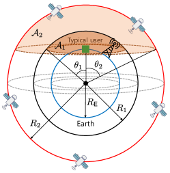
In our network model, we assume that the locations of base stations (BSs) for cellular and satellite networks are placed on the surface of sphere with radius for as illustrated in Fig. 1. We also denote the locations of the th BS for the th tier network by . The locations of the BSs for the th tier network are assumed to be distributed according to homogeneous PPPs with density . Therefore, the number of BSs on , , follows a Poisson distribution with mean .
Downlink users are assumed to be located on the surface of the Earth with radius , i.e., . The locations of the users are distributed according to a homogeneous PPP with density on , where is the location of the th user and is the number of users that follows a Poisson distribution with mean .
Our model differs from the classical cellular network model, in which the locations of the BSs and users are distributed in a two-dimensional plane . Whereas, in our model, the BSs and users are located on the surface of the spheres with different radii, which incorporates the curvature of the Earth.
Typical spherical cap and visible region: Under the premise that and follow homogeneous PPPs on the concentric spheres for and , the statistical distribution of with respect to any element in remains invariant under rotation. Leveraging Slivnyak’s theorem [34], we can, without loss of generality, focus on a typical user positioned at . As depicted in Fig. 1, we denote the typical spherical cap of the th network by . This typical spherical cap is defined as the field of view at the typical receiver’s location with the visible elevation angle as
| (2) |
where is the maximum visible elevation angle.
Without loss of generality, our attention is directed toward the downlink user performance within the confines of the typical spherical cap. It is essential to highlight that, exclusive to the typical user, only BSs positioned within the typical spherical cap for are observable. The spatial distributions of these visible cellular and satellite BSs are identical to the homogeneous PPPs with density .
II-B Channel and Antenna Gain Model
The propagation through the wireless channel is modeled by the combination of path-loss attenuation, shadowing, and small-scale fading effects.
Path-loss model: The path-loss model is dependent on the distance from the th BS of the th tier located at for to the typical user located at as
| (3) |
where is the path loss exponent. We assume a higher path loss exponent for cellular networks than satellite networks due to their distinct channel propagation characteristics. Cellular networks typically navigate urban communication scenarios characterized by rich scattering, necessitating a higher path loss exponent. In contrast, satellite networks predominantly operate in line-of-sight (LOS) scenarios, prompting a lower path loss exponent. Notably, the flexibility to adjust these path loss exponents independently for each tier enhances adaptability to diverse network conditions.
Antenna gain model: We assume that all BSs in the cellular and satellite networks adopt directional beamforming. For analysis tractability, we use a simple two-level antenna gain model wherein the main lobe is confined within the beamwidth, and the side lobe provides a reduced beam gain compared to the main lobe. We denote the main and side lobe antenna gains for the BSs in the th tier network by and . Assuming that BS in the th tier network is catering to the downlink user through main lobe beam alignment, while the beams of the interfering links are oriented towards the side lobe angles, the modeled effective beam gain is expressed as follows:
| (4) |
where and denote the main and side lobe beam gains of the downlink users. This simple two-lobe antenna gain model allows the analysis to be more tractable, and its effectiveness becomes particularly pronounced when coupled with sophisticated beam pattern techniques, such as Dolph-Chebyshev beamforming weights [42].
Fading model: For satellite links, we use the shadowed-Rician fading model, a time-honored fading model that captures land mobile satellite (LMS) links. Let be the fading power from the th BS of the th tier to the typical user. The probability density function (PDF) of is given by [43]
| (5) |
where is the Pochhammer symbol, , , and . Here, denotes the shape parameter of the Nakagami- distribution. Also, and are the average power of the LoS and multi-path components of the th tier downlink channel, respectively. Then, the cumulative distribution function (CDF) of is given by
| (6) |
where is the lower incomplete gamma function. The shadowed-Rician fading model exhibits remarkable versatility. Notably, the Nakagami- fading emerges as a special case of shadowed-Rician fading by setting the parameter to sufficiently small values. In our analysis, we leverage both the shadowed-Rician and Nakagami- channel fading models for the satellite and terrestrial channels, respectively.
II-C Flexible Network Association for Data Offloading
We propose an open access policy for facilitating flexible network association, wherein a downlink user can establish connections with all -tier networks, each equipped with orthogonal frequency bands. For a typical downlink user positioned at , first measures the effective ERP from the nearest BS within the th tier, located at with bias factor as
| (7) |
where is the transmit power of the BS in the th tier and denotes the average channel fading gain of the th tier. The latter encompasses distinct values for shadowed-Rician satellite channels and the Nakagami- terrestrial channel. The bias factor plays a crucial role in influencing the dynamics of data offloading in multi-tier networks. Downlink users tend to be naturally inclined towards connecting to terrestrial networks without using the bias factor, owing to their inherently larger ERP than satellite networks. To serve more users, satellite network operators may adjust the bias factor upwards, enhancing the ERP and favoring satellite connections.
After measuring the ERP, the downlink user chooses the best network that produces the highest ERP as
| (8) |
II-D Performance Metric
Let be a random variable indicating the connected network index. Given that the typical downlink user is linked to the th network, i.e., , we first define the coverage probability. As the downlink user is served by the closest BS in the th tier, placed at , the signal-to-interference-plus-noise ratio (SINR) of the typical downlink user positioned at is
| (9) |
where is the normalized noise power of the th tier and is the normalized antenna gain. Notice there is no cross-tier interference because all networks are assumed to use orthogonal frequency bands. The probability that the instantaneous SINR of the typical downlink user from the th tier is greater than a target SINR is defined as
| (10) |
Since the typical user is associated with at most one tier, from the law of total probability, the coverage probability of the th tier network under the open access policy is given as
| (11) |
where the network association probability is defined as
| (12) |
This network association probability is chiefly determined by the nearest distribution of the BS in each tier, i.e., the density of the network and the bias factors for . In this paper, we shall characterize the coverage probability in (11) and provide a system design guideline for optimizing the network parameters, such as the network densities and bias factors.
III Preliminaries
In this section, we introduce some useful lemmas that are essential for establishing the coverage probability expressions.
III-A Geometry Transform from a Spherical Cap to a Ring
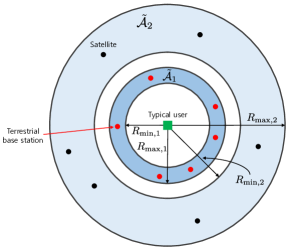
We introduce a displacement lemma that transforms the point process in a visible spherical cap into the point process in a projected ring. To explain this, we define a circular ring centered at with outer and inner radii, denoted as and as illustrated in Fig. 2. Let be a homogeneous PPP on with density .
Lemma 1.
The distance distributions from a typical user are preserved between on with density and on with density , provided that
| (13) |
Proof.
See [44]. ∎
Applying this geometry transformation lemma allows us to leverage more straightforward geometric intuition to analyze the coverage probability of sophisticated -tier ISTNs.
III-B First Touch Distribution
The distribution of the nearest BS from the typical downlink user is a key ingredient in analyzing the coverage probability. The following lemma elucidates the first-touch distribution within the transformed geometry. Unlike the traditional cellular networks modeled in , our network model using the transformed geometry on the ring requires computing the nearest BS’s distance distribution conditioned that one BS at least exists in the ring. The void probability for on is
| (14) |
From the void probability, the following lemmas describes the conditional first-touch distribution of the BS on .
Lemma 2.
Let be the distance from a typical user to the nearest BS of the th tier. Then, the PDF of conditioned on that at least one BS is visible is obtained as
| (15) |
Proof.
See Appendix A. ∎
This PDF will be a key role in computing the coverage probability of the th tier network.
III-C Network Connection Probability
By the open access policy, we assume that the typical downlink user is connected to the network generating the highest ERP in (7). The subsequent lemmas elucidate the probability of network connection contingent upon the maximum ERP under the open access policy.
Lemma 3.
The probability that a typical user is associated with the th tier conditioned on that at least one BS is visible in the th tier is
| (16) |
where
| (17) |
| (18) |
with
| (19) |
Proof.
See Appendix B. ∎
Lemma 4.
When a typical user is associated with the th tier, the PDF of conditioned on that at least one BS is visible is
| (20) |
Proof.
See Appendix C. ∎
These lemmas show how the network connection probability changes in terms of the critical system parameters including the network densities , the normalized bias factors , the normalized path-loss exponents , the normalized transmit power , and the normalized average fading power .
III-D Interference Laplace
The analysis of the coverage probability of ISTNs relies significantly on understanding the distribution of the aggregated interference, specifically the intra-tier interference power. The subsequent lemma elucidates the Laplace transform of the aggregated interference power, providing a crucial insight into the overall performance of ISTNs.
Lemma 5.
Let be the aggregated interference power of the th tier as
| (21) |
Then, the Laplace transform of the aggregated interference power plus normalized noise variance of the th tier conditioned on that at least one BS is on annulus is obtained as
| (22) |
Proof.
See Appendix D. ∎
The aggregated interference power is significantly influenced by the fading distribution of the interfering links and the density . For instance, as the network density decreases, the interference Laplace increases, which helps to improve the coverage probability. However, the proximity distribution of the BS worsens as the network density scales down, posing a detrimental impact on the coverage probability.
IV Coverage Probability
In this section, we first present the exact expression for the coverage probability of the -tier ISTNs. Unfortunately, the exact expression is challenging for analytical computation due to its involvement with intricate integrals. To address this complexity, we introduce an approximate expression for the coverage probability, specifically designed to be computed with significantly less intricacy, particularly under predefined conditions.
IV-A Exact Expression
The following theorem is the main result of this paper.
Theorem 1.
Proof.
See Appendix E. ∎
Our first key observation is the difference from [16] in the interference-limited regime. In [16], the coverage probability does not depend on the density of BSs when noise is ignored. Even in the interference-limited regime, the coverage probability varies depending on the density of BSs. This captures a realistic environment by modeling the terrestrial network on the sphere of the Earth. Intuitively, since the sum of the probabilities of being associated with the th tier of Lemma 19 is 1 for all tiers, the coverage probability of Theorem 1 may be considered an internally dividing point for every single tier at first glance. However, due to the difference in conditional nearest BS distance distribution between Lemmas 2 and 4 for single tier and multi-tier, Theorem 1 properly reflects the effect of macro-diversity that occurs by cooperating multiple networks. This is because when an outage occurs in one network, there is still a possibility that communication can succeed in the remaining networks. This possibility is reflected in terms of different tiers in Lemma 4. Therefore, as the number of tiers increases, the effect of macro-diversity increases because they do not share a spectrum. This macro-diversity effect is verified through simulation results in Section V.
IV-B Approximated Expression
The exact expression of Theorem 1 is computationally expensive when is large due to the derivative of . Therefore, we also provide an approximated form of the coverage probability.
Theorem 2.
The approximated coverage probability of the typical user conditioned on that a typical user is associated with the th tier and at least one BS is visible in the th tier is obtained as
| (25) |
where , and is the tuning parameter. This tuning parameter is adjustable only in the range of
| (26) |
Proof.
See Appendix F. ∎
This approximated form can be calculated faster than the exact form as becomes larger. Therefore, the approximated expression can be useful in environment where shadowing is not heavy. However, the approximation is very close to the exact form, and we verify how close it is through simulation results in Section V.
IV-C Special Case
To provide more clear intuition on the derived coverage probability expressions, we establish the approximated expression of the coverage probability in some special cases, which is stated in the following corollary.
Corollary 1.
When with and , , and are distributed as Rayleigh, the coverage probability in the interference-limited regime is approximated as
| (27) |
where and . In addition, , , , and . Furthermore,
| (28) |
and
| (29) |
where is an arbitrary correction constant for approximation.
Proof.
Corollary 1 provides valuable insights into how the coverage probability varies with critical network parameters. Similar to the prior result in [32], which is an alliterative analytical expression of Corollary 1, we note that in each network tier, the optimal density of satellite nodes for maximizing coverage probability diminishes with increasing network altitude. This result suggests that terrestrial networks necessitate a higher density of BSs than satellite networks to enhance coverage probability effectively.
Furthermore, Corollary 1 elucidates the impact of the biasing factor on network density. Essentially, increasing the biasing factor from 1 to can be conceptualized as adjusting the network density from to . Consequently, elevating the biasing factor in each tier effectively amplifies network density, thereby augmenting the likelihood of network connection for typical users. This observation resonates with our intuitive understanding of the biasing factor. The simulation section will provide a more detailed exploration of the biasing effect.
V Simulation Results
In this section, we validate our derived expressions for the Theorem through a comparison with Monte Carlo simulations. The shadowed-Rician fading, employed as the fading channel model in our study, offers versatility by reflecting various fading channels based on parameter configurations. Consequently, we employ Rayleigh fading for the terrestrial network and the LMS channel parameters specified in Table I for the satellite network. Given our assumption that is an integer, we adjust the actual LMS channel parameters to the nearest integer value for . Unless explicitly mentioned otherwise, we utilize the parameters listed in Table I for our simulations.
For the parameters pertaining to the satellite network, we draw upon values extracted from the link budget filed with the FCC [45]. This filing was submitted by SpaceX for the operation of a direct-to-cellular system. Notably, we assume omnidirectional reception for users’ antennas with a gain set to 0 dBi, denoted as . Our simulation is structured in two tiers to elucidate discernible trends, although it is inherently adaptable to multiple tiers without loss of generality.
| Parameter | Terrestrial | Satellite |
| Carrier frequency [GHz] | 3.5 | 1.9925 |
| Radius of the Earth [km] | 6371 | |
| Path-loss exponent | 4 | 2 |
| Speed of light [km/s] | ||
| Noise spectral density [dBm/Hz] | -174 | |
| Tx antenna gain for desired link [dBi] | 0 | 38 |
| Tx antenna gain for interference [dBi] | 0 | 28 |
| Tx power [dBm] | 46 | 50 |
| Bandwidth [MHz] | 100 | 5 |
| Altitude [km] | 0.03 | 530 |
| Visible elevation angle [rad] | ||
| LMS Channel Parameters [43] | |||
|---|---|---|---|
| Shadowing | |||
| Frequent Heavy Shadowing (FHS) | 1 | 0.063 | |
| Average Shadowing (AS) | 10 | 0.126 | 0.835 |
| Infrequent light Shadowing (ILS) | 19 | 0.158 | 1.29 |
V-A Network Model Validation
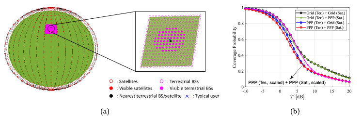
To validate the proposed ISTN model, we compare our PPP-based ISTN model with the classical grid network model, as shown in Fig. 3-(a). We consider the Walker star constellation for terrestrial and satellite networks in a grid model. Therefore, our grid model differs from the grid model in [16] in that the height of the terrestrial BS is considered. In the grid model, we assumed that a typical user is randomly located in the area where the reference satellite is the nearest. Therefore, once the user’s location is determined, the user is served by the reference satellite or the nearest terrestrial BS. Because the number of visible satellites and terrestrial BSs varies depending on the location of a typical user, we set the density in the PPP-based model to the average value of several snapshots.
Fig. 3-(b) shows simulation results for four possible combinations of grid- and PPP-based satellite and terrestial network models. As mentioned in [16], the distance between the nearest BS and interference BSs may be close in the PPP-based model, while the grid model ensures that a certain distance separates interference BSs. Therefore, unless the grid spacing is very close, the PPP-based model can serve as the lower bound on the coverage probability for the grid model, as shown in Fig. 3-(b). Both models have similar coverage tendencies, which validates our PPP-based network model. Additionally, we can similarly match the coverage probability in low SINR threshold regions by adjusting the density of the network. We also emphasize that the PPP-based satellite network model has shown to be accurate for analyzing the commercial LEO satellite network such as Starlink [32].
V-B Verification and Effect of Shadowing
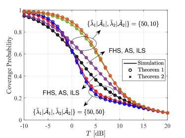
Fig. 4 shows the simulation results to verify Theorem 1 and 26 according to shadowing and satellite density. The analytical expressions derived in Theorem 1 and 26 perfectly match and are close to the simulation results. When , that is, FHS is considered, the approximated coverage probability matches well with the exact expression of the coverage probability. Therefore, Theorem 1 and 26 are identical for FHS. However, if , approximation error occurs no matter how well is adjusted. For AS and ILS, although the approximation errors occur, they are negligible and allow us to obtain coverage probabilities faster than exact form with lower computational complexity.
When , in the low SINR threshold region, coverage increases as shadowing becomes lighter, that is, as the LMS channel parameters , , and increases. This is because the influence of the nearest BS is greater than the interference in a low SINR threshold region. Therefore, a light shadowing environment with a strong LoS path of the nearest BS shows better performance. However, this tendency acts in the opposite direction above a certain SINR threshold, which is due to interference. Interference from satellites other than the nearest BS in a light shadowing environment reduces coverage probability. On the other hand, when , in all SINR threshold regions, the coverage probability is highest in ILS and lowest in FHS because the number of satellites acting as interference is small from the first.
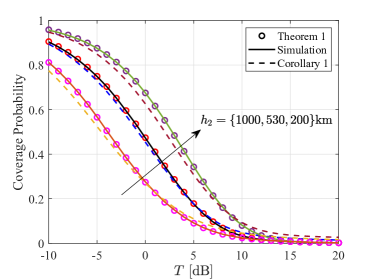
Fig. 5 shows the simulation results to verify Corollary 28 according to the altitude of the satellite. We set the simulation parameters as for km, for km, and for km. Compared to the exact form, the coverage probability derived in Corollary 28 exhibits similar trends, which shows the tightness of the derived closed form expression in some special cases. As can be seen, we show that lowering satellite altitude provides a higher coverage performance gain for ISTNs.
V-C Effects of Biasing and Density
As can be seen in Fig. 4, the coverage trend depends not only on the channel parameters but also on the density. Additionally, the main parameter that determines coverage performance is the biasing factor. Therefore, we provide simulation results to examine the influence of these two parameters on coverage performance. In this subsection, AS is considered for shadowing.
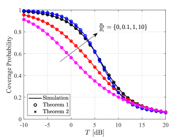
The simulation results depicted in Fig. 6 illustrate the impact of varying biasing factor ratios. A ratio of 0 signifies exclusive consideration of the terrestrial network, while higher ratios denote increased user association with the satellite network. In the terrestrial network, Rayleigh fading () is taken into account. When the biasing factor ratio is 0, aligning with the terrestrial network alone, Theorems 1 and 26 yield identical results. At a ratio of 0.1, predominantly terrestrial network associations prevail due to its higher biasing factor, leading to a close match between the theorems. However, as the biasing factor tilts towards the satellite network, there’s a threshold beyond which Theorem 26 diverges slightly from Theorem 1, though still exhibiting notable consistency. Particularly, when and , indicating a relatively lower satellite density compared to terrestrial BS, prioritizing collaboration with less interference-prone satellite networks is advisable.
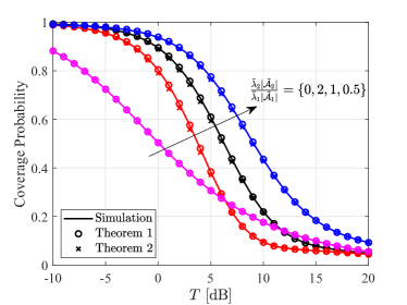
Next, Fig. 7 illustrates the simulation results based on the density ratio. Similar to Fig. 6, a ratio of 0 indicates consideration solely of the terrestrial network. When the density ratio is 0.5, the coverage performance surpasses that of the terrestrial network alone across all SINR thresholds . Conversely, at density ratios of 1 and 2, beyond a certain threshold, the collaboration of both networks exhibits diminished coverage probability due to increasing interference from additional satellites. However, given the generally higher coverage probability across most threshold ranges, integrating both networks would be advantageous for most systems. As observed in Fig. 6 and Fig. 7, coverage varies depending on the biasing factor and density, suggesting an optimal ratio for these parameters to maximize coverage under different circumstances.
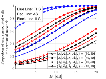
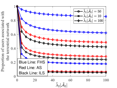
Fig. 8 and Fig. 9 depict the proportion of users linked to the terrestrial network based on key parameters such as shadowing, biasing factor, and density. Specifically, Fig. 8 illustrates how the proportion of users associated with the terrestrial network varies with the biasing factor of the terrestrial network across different shadowing and density scenarios. A higher value of implies a greater bias towards the terrestrial network, consequently leading to an increase in the proportion of users associated with it. Essentially, lighter shadowing corresponds to a stronger LOS path power. Therefore, under similar density conditions, the proportion of users associated with the terrestrial network is highest in scenarios with FHS and lowest in scenarios with Infrequent Light Shadowing ILS. This trend arises because a higher biasing factor amplifies the influence of the terrestrial network, making it more attractive to users. Moreover, in environments with high network density, a significant portion of users tends to be associated with networks exhibiting greater density. Notably, the density of terrestrial BSs significantly impacts the distribution of users among networks, highlighting the sensitivity of terrestrial BS density to the proportion of users associated with each network.
Fig. 9 illustrates how the proportion of users linked with the terrestrial network varies concerning the satellite density across different terrestrial base station densities. Comparably, Fig. 8 echoes this trend, revealing that the highest proportion of users affiliated with the terrestrial network occurs in FHS scenarios, while the lowest is observed in ILS scenarios, all under identical terrestrial base station densities. Evidently, with an escalation in satellite density, there is a corresponding increase in the proportion of users associated with the satellite network. However, as depicted in the case of , this proportion reaches a saturation point beyond a certain satellite density. Moreover, the density of terrestrial base stations also significantly influences the proportion of users linked to the terrestrial network. Consequently, both the terrestrial and satellite network densities exert substantial impacts on coverage metrics.
VI Conclusion
In this paper, we have introduced a analytical method for assessing downlink coverage performance of the -tier ISTNs. Our approach involves modeling the spatial distribution of BSs of each network tier using homogeneous PPPs on concentric spheres. This modeling accommodates multiple tiers within both terrestrial and satellite networks while maintaining identical network geometry shapes. Under this unified network model, we have derived the expressions for the downlink coverage probability of ISTNs, incorporating essential network design parameters such as network density, path-loss exponent, fading parameters, and network association bias factors. Through simulations, we validate the accuracy of these derived expressions and analyze the impacts of various network parameters. Our tractable approach provides valuable insights for system design and parameter optimization in multi-band ISTN deployment, facilitating informed decision-making and efficient network management.
Appendix A Proof of Lemma 2
The conditional nearest BS distance distribution of the th tier can be calculated from the complementary cumulative distribution function (CCDF) conditioned on that . Let be the distance between the typical user and the nearest BS of the th tier. The conditional CCDF of the nearest BS distance of the th tier can be obtained as
| (30) |
where is the partial spherical cap defined as
| (31) |
(a) is by Bayes’ theorem, (b) follows from the independence between disjoint sets and and (c) is by the void probability of Lemma 1. The conditional nearest BS distance distribution of the th tier can be calculated by taking the derivative with respect to , which completes the proof.
Appendix B Proof of Lemma 19
In order for a typical user to be associated with the th tier, the ERP of the th tier must be the largest. Namely, for all . Therefore, Lemma 19 is calculated as
| (32) |
In our model, because there is a range in which the BS can be located, the probability in the last equation varies depending on . The interval of integration is divided into three cases according to the following conditions:
| (33) |
Therefore,
| (34) |
where
| (35) |
When , , , and
| (36) |
As a result,
| (37) |
Appendix C Proof of Lemma 4
We start by finding the conditional CCDF similar to the proof of Lemma 2 in Appendix A. Therefore,
| (38) |
The joint probability that and a typical user is associated with the th tier is
| (39) |
We can obtain the PDF of conditioned on that a typical user is associated with the th tier and at least one BS is visible in the th tier by differentiating the conditional CDF as
| (40) |
for .
Appendix D Proof of Lemma 5
We first assume that the distance from the nearest BS of the th tier to typical user is . Therefore, the condition for this distance from typical user to nearest BS is also additionally required. As a result, the Laplace transform of the aggregated interference plus noise power conditioned on that the distance from a typical user to the nearest BS of the th tier is and at least one BS exist in the annulus is calculated as
| (41) |
where (a) follows from a Laplace functional of the PPP [35], which is also known as the probability generating functional (PGFL) of the PPP [46], (b) is applied the moment generating function (MGF) of the shadowed-Rician fading [43], and (c) is the conversion of the area corresponding to the surface area of the annulus into polar coordinates.
Appendix E Proof of Theorem 1
We consider the conditional coverage probability according to all possible distances from a typical user to the nearest BS of the th tier, i.e., take the expected value for the nearest BS distance . Additionally, since the aggregated interference power of the th tier is also a random variable, we also average over the aggregated interference power . Namely, the conditional coverage probability is calculated as
| (42) |
where is the distance from the nearest BS of the th tier to the typical user. Using the CDF of the shadowed-Rician fading in (6), the CCDF of is obtained as
| (43) |
The lower incomplete gamma function in (43) can be rewritten as
| (44) |
Therefore, we can also rewrite the CCDF of in (43) as
| (45) |
Using this CCDF of (43), the conditional coverage probability in (42) can be specifically calculated as
| (46) |
where (a) is because the average is taken for , and (b) comes from the derivative property of the Laplace transform with and the Laplace transform of the aggregated interference power plus normalized noise variance is obtained in Lemma 5.
Appendix F Proof of Theorem 26
We start with the lower and upper bounds of the lower incomplete gamma function as
| (47) |
These lower and upper bounds form another inequality as
| (48) |
Depending on , the lower incomplete gamma function can be approximated as
| (49) |
When , and the equality holds. However, when , must be tuned to be as similar as possible.
References
- [1] I. Del Portillo, B. G. Cameron, and E. F. Crawley, “A technical comparison of three low earth orbit satellite constellation systems to provide global broadband,” Acta Astronaut., vol. 159, pp. 123–135, Jun. 2019.
- [2] A. Guidotti, A. Vanelli-Coralli, M. Caus, J. Bas, G. Colavolpe, T. Foggi, S. Cioni, A. Modenini, and D. Tarchi, “Satellite-enabled lte systems in leo constellations,” in 2017 IEEE Int. Conf. Commun. Workshops (ICC Workshops). IEEE, Jul. 2017, pp. 876–881.
- [3] S. Cioni, R. De Gaudenzi, O. D. R. Herrero, and N. Girault, “On the satellite role in the era of 5g massive machine type communications,” IEEE Netw., vol. 32, no. 5, pp. 54–61, Sep. 2018.
- [4] A. Guidotti, A. Vanelli-Coralli, M. Conti, S. Andrenacci, S. Chatzinotas, N. Maturo, B. Evans, A. Awoseyila, A. Ugolini, T. Foggi et al., “Architectures and key technical challenges for 5g systems incorporating satellites,” IEEE Trans. Veh. Technol., vol. 68, no. 3, pp. 2624–2639, Mar. 2019.
- [5] X. Lin, S. Cioni, G. Charbit, N. Chuberre, S. Hellsten, and J.-F. Boutillon, “On the path to 6g: Embracing the next wave of low earth orbit satellite access,” IEEE Commun. Mag., vol. 59, no. 12, pp. 36–42, Dec. 2021.
- [6] P. Yang, Y. Xiao, M. Xiao, and S. Li, “6g wireless communications: Vision and potential techniques,” IEEE Netw., vol. 33, no. 4, pp. 70–75, Jul. 2019.
- [7] Z. Zhang, Y. Xiao, Z. Ma, M. Xiao, Z. Ding, X. Lei, G. K. Karagiannidis, and P. Fan, “6g wireless networks: Vision, requirements, architecture, and key technologies,” IEEE Veh. Technol. Mag., vol. 14, no. 3, pp. 28–41, Sep. 2019.
- [8] Y. Qian, “Integrated terrestrial-satellite communication networks and services,” IEEE Wirel. Commun., vol. 27, no. 6, pp. 2–3, Dec. 2020.
- [9] L. Qian, P. Yang, Y. L. Guan, Z. Liu, Y. Xiao, K. Jiang, and M. Xiao, “Multi-dimensional polarized modulation for land mobile satellite communications,” IEEE Trans. Cogn. Commun. Netw., vol. 7, no. 2, pp. 383–397, Jun. 2021.
- [10] “5g and non-terrestrial networks,” 5G americas, White paper, Feb. 2022, available: https://www.5gamericas.org/5g-americas-releases-update-on-5g-non-terrestrial-networks/.
- [11] B. Al Homssi, A. Al-Hourani, K. Wang, P. Conder, S. Kandeepan, J. Choi, B. Allen, and B. Moores, “Next generation mega satellite networks for access equality: Opportunities, challenges, and performance,” IEEE Commun. Mag., vol. 60, no. 4, pp. 18–24, Apr. 2022.
- [12] F. Baccelli, B. Blaszczyszyn, and P. Muhlethaler, “An aloha protocol for multihop mobile wireless networks,” IEEE Trans. Inf. Theory, vol. 52, no. 2, pp. 421–436, Jan. 2006.
- [13] N. Lee, X. Lin, J. G. Andrews, and R. W. Heath, “Power control for d2d underlaid cellular networks: Modeling, algorithms, and analysis,” IEEE J. Sel. Areas Commun., vol. 33, no. 1, pp. 1–13, Nov. 2014.
- [14] A. Al-Hourani, S. Kandeepan, and A. Jamalipour, “Stochastic geometry study on device-to-device communication as a disaster relief solution,” IEEE Trans. Veh. Technol., vol. 65, no. 5, pp. 3005–3017, May 2016.
- [15] Y. J. Chun, S. L. Cotton, H. S. Dhillon, A. Ghrayeb, and M. O. Hasna, “A stochastic geometric analysis of device-to-device communications operating over generalized fading channels,” IEEE Trans. Wirel. Commun., vol. 16, no. 7, pp. 4151–4165, Mar. 2017.
- [16] J. G. Andrews, F. Baccelli, and R. K. Ganti, “A tractable approach to coverage and rate in cellular networks,” IEEE Trans. Commun., vol. 59, no. 11, pp. 3122–3134, Oct. 2011.
- [17] H. S. Dhillon, R. K. Ganti, F. Baccelli, and J. G. Andrews, “Modeling and analysis of k-tier downlink heterogeneous cellular networks,” IEEE J. Sel. Areas Commun., vol. 30, no. 3, pp. 550–560, Mar. 2012.
- [18] H.-S. Jo, Y. J. Sang, P. Xia, and J. G. Andrews, “Heterogeneous cellular networks with flexible cell association: A comprehensive downlink sinr analysis,” IEEE Trans. Wirel. Commun., vol. 11, no. 10, pp. 3484–3495, Oct. 2012.
- [19] K. Huang and J. G. Andrews, “An analytical framework for multicell cooperation via stochastic geometry and large deviations,” IEEE Trans. Inf. Theory, vol. 59, no. 4, pp. 2501–2516, Dec. 2012.
- [20] N. Lee, D. Morales-Jimenez, A. Lozano, and R. W. Heath, “Spectral efficiency of dynamic coordinated beamforming: A stochastic geometry approach,” IEEE Trans. Wirel. Commun., vol. 14, no. 1, pp. 230–241, Jul. 2014.
- [21] T. Bai, A. Alkhateeb, and R. W. Heath, “Coverage and capacity of millimeter-wave cellular networks,” IEEE Commun. Mag., vol. 52, no. 9, pp. 70–77, Sep. 2014.
- [22] M. Di Renzo, “Stochastic geometry modeling and analysis of multi-tier millimeter wave cellular networks,” IEEE Trans. Wirel. Commun., vol. 14, no. 9, pp. 5038–5057, May 2015.
- [23] J. Park, N. Lee, J. G. Andrews, and R. W. Heath, “On the optimal feedback rate in interference-limited multi-antenna cellular systems,” IEEE Trans. Wirel. Commun., vol. 15, no. 8, pp. 5748–5762, May 2016.
- [24] J. Park, J. G. Andrews, and R. W. Heath, “Inter-operator base station coordination in spectrum-shared millimeter wave cellular networks,” IEEE Trans. Cogn. Commun. Netw., vol. 4, no. 3, pp. 513–528, Mar. 2018.
- [25] R. Wang, M. A. Kishk, and M.-S. Alouini, “Resident population density-inspired deployment of k-tier aerial cellular network,” IEEE Trans. Wirel. Commun., Mar. 2023.
- [26] A. Talgat, M. A. Kishk, and M.-S. Alouini, “Stochastic geometry-based analysis of leo satellite communication systems,” IEEE Commun. Lett., vol. 25, no. 8, pp. 2458–2462, Oct. 2020.
- [27] N. Okati, T. Riihonen, D. Korpi, I. Angervuori, and R. Wichman, “Downlink coverage and rate analysis of low earth orbit satellite constellations using stochastic geometry,” IEEE Trans. Commun., vol. 68, no. 8, pp. 5120–5134, Apr. 2020.
- [28] N. Okati and T. Riihonen, “Nonhomogeneous stochastic geometry analysis of massive leo communication constellations,” IEEE Trans. Commun., vol. 70, no. 3, pp. 1848–1860, Jan. 2022.
- [29] A. Al-Hourani, “An analytic approach for modeling the coverage performance of dense satellite networks,” IEEE Wirel. Commun. Lett., vol. 10, no. 4, pp. 897–901, Jan. 2021.
- [30] ——, “Optimal satellite constellation altitude for maximal coverage,” IEEE Wirel. Commun. Lett., vol. 10, no. 7, pp. 1444–1448, Mar. 2021.
- [31] D.-H. Na, K.-H. Park, Y.-C. Ko, and M.-S. Alouini, “Performance analysis of satellite communication systems with randomly located ground users,” IEEE Trans. Wirel. Commun., vol. 21, no. 1, pp. 621–634, Jul. 2021.
- [32] J. Park, J. Choi, and N. Lee, “A tractable approach to coverage analysis in downlink satellite networks,” IEEE Trans. Wirel. Commun., Aug. 2022.
- [33] K. S. Gilhousen, I. M. Jacobs, R. Padovani, A. J. Viterbi, L. A. Weaver, and C. E. Wheatley, “On the capacity of a cellular cdma system,” IEEE Trans. Veh. Technol., vol. 40, no. 2, pp. 303–312, May 1991.
- [34] A. J. Viterbi, A. M. Viterbi, and E. Zehavi, “Other-cell interference in cellular power-controlled cdma,” IEEE Trans. Commun., vol. 42, no. 234, pp. 1501–1504, Feb.-Apr. 1994.
- [35] M. Haenggi, J. G. Andrews, F. Baccelli, O. Dousse, and M. Franceschetti, “Stochastic geometry and random graphs for the analysis and design of wireless networks,” IEEE J. Sel. Areas Commun., vol. 27, no. 7, pp. 1029–1046, Aug. 2009.
- [36] S. N. Chiu, D. Stoyan, W. S. Kendall, and J. Mecke, Stochastic geometry and its applications. John Wiley & Sons, 2013.
- [37] R. Wang, M. A. Kishk, and M.-S. Alouini, “Ultra-dense leo satellite-based communication systems: A novel modeling technique,” IEEE Commun. Mag., vol. 60, no. 4, pp. 25–31, Apr. 2022.
- [38] ——, “Evaluating the accuracy of stochastic geometry based models for leo satellite networks analysis,” IEEE Commun. Lett., vol. 26, no. 10, pp. 2440–2444, Jul. 2022.
- [39] Z. Song, J. An, G. Pan, S. Wang, H. Zhang, Y. Chen, and M.-S. Alouini, “Cooperative satellite-aerial-terrestrial systems: A stochastic geometry model,” IEEE Trans. Wirel. Commun., vol. 22, no. 1, pp. 220–236, Jul. 2022.
- [40] B. Al Homssi and A. Al-Hourani, “Modeling uplink coverage performance in hybrid satellite-terrestrial networks,” IEEE Commun. Lett., vol. 25, no. 10, pp. 3239–3243, Aug. 2021.
- [41] J. Park, J. Choi, N. Lee, and F. Baccelli, “Unified modeling and rate coverage analysis for satellite-terrestrial integrated networks: Coverage extension or data offloading?” arXiv preprint arXiv:2307.03343, 2023.
- [42] C. L. Dolph, “A current distribution for broadside arrays which optimizes the relationship between beam width and side-lobe level,” Proc. IRE, vol. 34, no. 6, pp. 335–348, Jun. 1946.
- [43] A. Abdi, W. C. Lau, M.-S. Alouini, and M. Kaveh, “A new simple model for land mobile satellite channels: First-and second-order statistics,” IEEE Trans. Wirel. Commun., vol. 2, no. 3, pp. 519–528, May 2003.
- [44] D. Kim, J. Park, and N. Lee, “Coverage analysis of dynamic coordinated beamforming for leo satellite downlink networks,” arXiv preprint arXiv:2309.10460, 2023.
- [45] Space Exploration Holdings, LLC, SpaceX Gen2 Direct-to-Cellular System FCC filing SAT-MOD-20230207-00021, [Online]. https://fcc.report/IBFS/SAT-MOD-20230207-00021.
- [46] M. Westcott, “The probability generating functional,” J. Aust. Math. Soc., vol. 14, no. 4, pp. 448–466, Dec. 1972.