Unbiased Parameter Estimation via DREM with Annihilators

Abstract

In the adaptive control theory, the dynamic regressor extension and mixing (DREM) procedure has become widespread as it allows one to describe a variety of adaptive control problems in unified terms of the parameter estimation problem of a regression equation with a scalar regressor. However, when the system/parameterization is affected by perturbations, the estimation laws, which are designed on the basis of such equation, asymptotically provides only biased estimates. In this paper, based on the bias-eliminated least-squares (BELS) approach, a modification of the DREM procedure is proposed that allows one to annihilate perturbations asymptotically and, consequently, asymptotically obtain unbiased estimates. The theoretical results are supported with mathematical modelling and can be used to design adaptive observers and control systems.

I Introduction

Using various parameterization schemes, the problems of controller and observer design for systems with a priori unknown parameters can be reduced to the one of online identification of the regression equation parameters:

$$z\left(t\right)={\varphi^{\top}}\left(t\right)\theta+w\left(t\right){\rm{,}}$$ (1)

where $z\left(t\right)\in\mathbb{R}$ and $\varphi\left(t\right)\in{\mathbb{R}^{n}}$ are measurable for all $t\geq{t_{0}}$ regressand and regressor, respectively, $\theta\in{\mathbb{R}^{n}}$ stands for unknown parameters, $w\left(t\right)\in\mathbb{R}$ denotes a bounded perturbation.

For example, in [1] the problem of adaptive output-feedback control of a linear time-invariant nonminimum-phase dynamic system is reduced to the one of the parameter identification, and in [2] the problem of state observer design for the same class of systems is also transformed into the same problem.

To reduce the regression equation (1) to a set of scalar regression equations, a dynamic regressor extension and mixing procedure (DREM) is proposed in [3], which consists of a dynamic extension step ($l>0$ is a filter parameter):

$$\begin{array}[]{l}\dot{Y}\left(t\right)=-lY\left(t\right)+\varphi\left(t\right)y\left(t\right){\rm{,\;}}Y\left({{t_{0}}}\right)={0_{n}}{\rm{,}}\\ \dot{\Phi}\left(t\right)=-l\Phi\left(t\right)+\varphi\left(t\right){\varphi^{\top}}\left(t\right){\rm{,\;}}\Phi\left({{t_{0}}}\right)={0_{n\times n}}{\rm{,}}\end{array}$$ (2a)

and mixing step

$${\cal Y}\left(t\right)={\rm{adj}}\left\{{\Phi\left(t\right)}\right\}Y\left(t\right).$$ (2b)

Together, equations (2a) and (2b) allow one to transform the regression equation (1) into a set of scalar ones:

$${{\cal Y}_{i}}\left(t\right)=\Delta\left(t\right){\theta_{i}}+{{\cal W}_{i}}\left(t\right){\rm{,}}$$ (3)

where

$$\begin{array}[]{c}{\cal Y}\left(t\right){\rm{:}}={\rm{adj}}\left\{{\Phi\left(t\right)}\right\}Y\left(t\right){\rm{,\;}}\Delta\left(t\right){\rm{:}}={\rm{det}}\left\{{\Phi\left(t\right)}\right\}{\rm{,}}\\ {\cal W}\left(t\right){\rm{:}}={\rm{adj}}\left\{{\Phi\left(t\right)}\right\}W\left(t\right){\rm{,}}\\ {\cal Y}\left(t\right)={{\begin{bmatrix}{{{\cal Y}_{1}}\left(t\right)}&\ldots&{{{\cal Y}_{i-1}}\left(t\right)}&{\begin{array}[]{*{20}{c}}\ldots&{{{\cal Y}_{n}}\left(t\right)}\end{array}}\end{bmatrix}}^{\top}}{\rm{,}}\\ {\cal W}\left(t\right)={{\begin{bmatrix}{{{\cal W}_{1}}\left(t\right)}&\ldots&{{{\cal W}_{i-1}}\left(t\right)}&{\begin{array}[]{*{20}{c}}\ldots&{{{\cal W}_{n}}\left(t\right)}\end{array}}\end{bmatrix}}^{\top}}{\rm{,}}\\ \dot{W}\left(t\right)=-lW\left(t\right)+\varphi\left(t\right)w\left(t\right){\rm{,\;}}W\left({{t_{0}}}\right)={0_{n}}.\end{array}$$

Based on the obtained system (3), each $i^{\rm th}$ unknown parameter can be identified independently using various identification laws. The degree of freedom of the procedure under consideration is the choice of a method to extend the regressor (2a). For example, instead of (2a), the following algorithms proposed respectively in [4, 5, 6] can also be used:

$$\begin{array}[]{l}\dot{Y}\left(t\right)={\textstyle{1\over T}}\left[{\varphi\left(t\right)z\left(t\right)-\varphi\left({t-T}\right)z\left({t-T}\right)}\right]{\rm{,}}\\ \dot{\Phi}\left(t\right)={\textstyle{1\over T}}\left[{\varphi\left(t\right){\varphi^{\top}}\left(t\right)-\varphi\left({t-T}\right){\varphi^{\top}}\left({t-T}\right)}\right]{\rm{,}}\end{array}$$ (4a)

$$Y\left(t\right)={\begin{bmatrix}{{{\cal H}_{1}}\left(s\right)z\left(t\right)}\\ {{{\cal H}_{2}}\left(s\right)z\left(t\right)}\\ \vdots\\ {{{\cal H}_{n}}\left(s\right)z\left(t\right)}\end{bmatrix}}{\rm{,\;}}\Phi\left(t\right)={\begin{bmatrix}{{{\cal H}_{1}}\left(s\right)\varphi\left(t\right)}\\ {{{\cal H}_{2}}\left(s\right)\varphi\left(t\right)}\\ \vdots\\ {{{\cal H}_{n}}\left(s\right)\varphi\left(t\right)}\end{bmatrix}}{\rm{,}}$$ (4b)

$$\begin{array}[]{l}\dot{Y}\left(t\right)=-\Gamma\varphi\left(t\right){\varphi^{\top}}\left(t\right)Y\left(t\right)+\Gamma\varphi\left(t\right)z\left(t\right){\rm{,}}\\ \Phi\left(t\right)={I_{n}}-\Sigma\left(t\right){\rm{,}}\\ \dot{\Sigma}\left(t\right)=-\Gamma\varphi\left(t\right){\varphi^{\top}}\left(t\right)\Sigma\left(t\right){\rm{,\;}}\Sigma\left({{t_{0}}}\right)={I_{n}}{\rm{,}}\end{array}$$ (4c)

where $T>0$ is the filtering window length, ${{\cal H}_{i}}\left(s\right)$ stands for an asymptotically stable linear filter (for instance, ${{\cal H}_{i}}\left(s\right)=\linebreak={\textstyle{1\over{s+{\alpha_{i}}}}}{\rm{,\;}}{\alpha_{i}}>0$), $\Gamma={\Gamma^{\top}}>0$ denotes an adaptive gain.

In [3, 6, 7], it is demonstrated that, when $w\left(t\right)\equiv 0$, the gradient-based identification law designed on the basis of equation (3) has a relaxed parametric convergence condition and improved transient quality compared to the gradient or least squares based laws designed using equation (1). In [3, 6, 7, 8, 9, 10, 11, 12, 13], various implementations of the DREM procedure have been proposed, which differ from each other mainly by the filters (e.g., (2a), (4a), (4b) or (4c), etc.) used for the regressor extension and/or the identification algorithms applied to estimate the $i^{\rm th}$ unknown parameter. The extension scheme defines the properties of the regressor $\Delta\left(t\right)$ and the perturbations ${\mathcal{W}}_{i}\left(t\right)$. For example, scheme (4c) strictly relaxes the regressor persistent excitation condition, which is required to ensure exponential convergence of the unknown parameter estimates [6]. Also, in [6], the identifiability conditions of the regression equation (3) parameters are investigated for the perturbation-free case. In [14], it is proved that the regressor $\varphi\left(t\right)$ excitation propagates to the scalar regressor $\Delta\left(t\right)$ when (2a) is used for the extension step. In [15], a similar property is shown for the scheme (4b). In [16], it is proved that the gradient-based identification law derived using equation (3) ensures asymptotical convergence to the unknown parameters if $\Delta\notin{L_{2}}$ and $\Delta{{\cal W}_{i}}\in{L_{1}}$. In [11, 12], boundedness of $\tilde{\theta}\left(t\right)$ was shown for ${{\cal W}_{i}}\in L_{2}$, and various estimation laws with finite time convergence and improved accuracy are developed for perturbed regressions. In [17], an identification law is proposed which, in contrast to [3, 6, 7, 8, 9, 10, 11, 12, 13, 14, 15, 16], ensures asymptotic identification of the unknown parameters when the averaging conditions (${{\cal W}_{i}}\in{L_{\infty}}$ and $\int\limits_{{t_{0}}}^{t}{{\Delta^{-1}}\left(s\right){{\cal W}_{i}}\left(s\right)ds<\infty}$) are met. In [18], different discrete laws, which provide improved accuracy of unknown parameter estimation in case of perturbations, are compared. In [19, 20], a new nonlinear filter is proposed, which ensures an arbitrary reduction of the steady-state parametric error under a certain regressor/perturbation ratio and independence of the regressor from the perturbation. In [21], based on the DREM procedure and the method of instrumental variables, an algorithm to identify the parameters of linear systems affected by external perturbations is developed that guarantees asymptotic convergence of the parametric error to zero. Unfortunately this approach is applicable only to estimate the linear system parameters.

The main and general drawback of [3, 6, 7, 8, 9, 10, 11, 12, 13, 14, 15, 16, 17, 18, 19, 20, 21] is that the parametric convergence conditions are formalized in terms of properties of the perturbation ${\cal W}\left(t\right)$ from the scalar regression equation (3). However, these conditions may never be met due to the features of the mixing procedure and the dynamic operators used at the extension step. For example, the averaging condition from [17] is not satisfied for all $i=\overline{1{\rm{,\;}}n}$, if the regressor $\varphi\left(t\right)$ elements are correlated with the perturbation $w\left(t\right)$ and among themselves. In this case, only biased estimates can be obtained asymptotically using the set of scalar regression equations (3). In this study, based on the bias-eliminated least-squares (BELS) approach [22, 23] previously applied for offline identification problems, a modified DREM procedure is proposed. In comparison with existing approaches [3, 6, 7, 8, 9, 10, 11, 12, 13, 14, 15, 16, 17, 18, 19, 20, 21], i) the obtained estimates converge to arbitrary neighborhood of ideal parameters if at least one element of the regressor $\varphi_{i}\left(t\right)$ is independent from the perturbation $w\left(t\right)$, ii) the main conditions of convergence are formalized in terms of the perturbation and regressor of the original regression equation (1).

II Problem Statement

The regression equation (1) is considered. The aim is to design an online estimation law, which, using the measurable signals $\varphi\left(\tau\right){\rm{,\;}}z\left(\tau\right){\rm{\;}}{t_{0}}\leq\tau\leq t$, ensures that the following conditions hold:

$$\mathop{{\rm{lim}}}\limits_{t\to\infty}\left\|{\tilde{\theta}\left(t\right)}\right\|\leq\varepsilon\left(T\right){\rm{,\;}}\mathop{{\rm{lim}}}\limits_{T\to\infty}\varepsilon\left(T\right)=0{\rm{,}}$$ (5)

where $T>0$ is some parameter of the identification algorithm, and $\varepsilon{\rm{:\;}}{\mathbb{R}_{+}}\mapsto{\mathbb{R}_{+}}$.

III Main result

In this section, a modified version of the DREM procedure [3, 7] is designed on the basis of the BELS approach [22, 23] previously applied for the discrete time and off-line identification. The convergence conditions of the new identifier will be obtained in terms of the regression equation (1), and the goal (5) will be achieved.

To introduce the proposed estimator we make some simple transformations of the linear regression equation (1). First of all, the linear dynamic filter ${\cal H}\left(s\right)={\textstyle{\alpha\over{s+\alpha}}}{\rm{,\;}}\alpha>0$ is applied to the left- and right-hand sides of equation (1):

$${z_{f}}\left(t\right)=\varphi_{f}^{\top}\left(t\right)\theta+{w_{f}}\left(t\right){\text{,}}$$ (6)

where

$$\begin{gathered}{z_{f}}\left(t\right){\text{:}}=\mathcal{H}\left(s\right)z\left(t\right){\text{,\;}}{\varphi_{f}}\left(t\right){\text{:}}=\mathcal{H}\left(s\right)\varphi\left(t\right){\text{,}}\;\\ {w_{f}}\left(t\right){\text{:}}=\mathcal{H}\left(s\right)w\left(t\right).\end{gathered}$$

Subtracting (6) from (1), it is obtained:

$$\tilde{z}\left(t\right)={\phi^{\top}}\left(t\right)\Theta+f\left(t\right){\rm{,}}$$ (7)

where

$$\begin{array}[]{c}\tilde{z}\left(t\right){\rm{:}}=z\left(t\right)-{z_{f}}\left(t\right){\rm{,}}\\ \phi\left(t\right){\rm{:}}={{\begin{bmatrix}{{\varphi^{\top}}\left(t\right)}&{\varphi_{f}^{\top}\left(t\right)}\end{bmatrix}}^{\top}}{\rm{,}}\\ f\left(t\right){\rm{:}}=w\left(t\right)-{w_{f}}\left(t\right){\rm{,\;}}\Theta{\rm{:}}={\begin{bmatrix}\theta\\ {-\theta}\end{bmatrix}}.\end{array}$$

In the next step equation (7) is extended via (4a):

$$\begin{array}[]{l}\dot{Y}\left(t\right)={\textstyle{1\over T}}\left[\phi\left(t\right){\tilde{z}\left(t\right)}-\phi\left({t-T}\right){\tilde{z}\left({t-T}\right)}\right]{\rm{,}}\\ \dot{\Phi}\left(t\right)={\textstyle{1\over T}}\left[{\phi\left(t\right){\phi^{\top}}\left(t\right)-\phi\left({t-T}\right){\phi^{\top}}\left({t-T}\right)}\right]{\rm{,}}\\ Y\left({{t_{0}}}\right)={0_{2n}}{\rm{,\;}}\Phi\left({{t_{0}}}\right)={0_{2n\times 2n}}.\end{array}$$ (8)

Owing to the implication

$$\begin{gathered}x\left(t\right)={\textstyle{1\over T}}\int\limits_{{\rm{max}}\left\{{{t_{0}}{\rm{,\;}}t-T}\right\}}^{t}{x\left(s\right)ds}\\ \Updownarrow\\ \dot{x}\left(t\right)={\textstyle{1\over T}}\left[{x\left(t\right)-x\left({t-T}\right)}\right]{\rm{,\;}}x\left({{t_{0}}}\right)=0{\rm{,}}\end{gathered}$$

the signals $Y\left(t\right)$ and $\Phi\left(t\right)$ meet the following relation:

$$Y\left(t\right)=\Phi\left(t\right)\Theta+W\left(t\right){\rm{,}}$$ (9)

where

$$\dot{W}\left(t\right)={\textstyle{1\over T}}\left[{\phi\left(t\right)f\left(t\right)-\phi\left({t-T}\right)f\left({t-T}\right)}\right]{\rm{,\;}}W\left({{t_{0}}}\right)={0_{2n}}.$$

Disturbance term in (9) always admits the decomposition:

$$W\left(t\right){\rm{:}}={{\cal L}_{1}}{\cal L}_{1}^{\top}W\left(t\right){\rm{+}}{{\cal L}_{2}}{\cal L}_{2}^{\top}W\left(t\right){\rm{,}}$$ (10)

where ${{\cal L}_{1}}\in{\mathbb{R}^{2n\times 2m}}$ and ${{\cal L}_{2}}\in{\mathbb{R}^{2n\times\left({2n-2m}\right)}}$ such that:

$$\begin{array}[]{c}{\cal L}_{1}^{\top}{{\cal L}_{1}}={I_{2m\times 2m}}{\rm{,\;}}{\cal L}_{2}^{\top}{{\cal L}_{2}}={I_{\left({2n-2m}\right)\times\left({2n-2m}\right)}}{\rm{,}}\\ {{\cal L}_{1}}{\cal L}_{1}^{\top}+{{\cal L}_{2}}{\cal L}_{2}^{\top}={I_{2n\times 2n}}{\rm{,}}\end{array}$$

and $2\left({n-m}\right)$ is the number of elements of the vector $\phi\left(t\right)$, for which the independence condition holds:

$$\mathop{{\rm{lim}}}\limits_{T\to\infty}{\textstyle{1\over T}}\int\limits_{{\rm{max}}\left\{{{t_{0}}{\rm{,\;}}t-T}\right\}}^{t}{{\phi_{i}}\left(s\right)f\left(s\right)ds}=0,\;\forall t\geq t_{0}.$$ (11)

For example, condition (11) is met for $\phi_{i}\left(t\right)=\linebreak={\rm{sin}}\left(\omega_{1}t+c_{1}\right)$ and $f\left(t\right)={\rm{sin}}\left(\omega_{2}t+c_{2}\right)$ iff $\omega_{1}\neq\omega_{2}$.

Multiplication (9) by ${\rm{adj}}\left\{{\Phi\left(t\right)}\right\}$ and substitution of (10) yields:

$${\cal Y}\left(t\right)=\Delta\left(t\right)\Theta+{{\cal W}_{1}}\left(t\right)+{{\cal W}_{2}}\left(t\right){\rm{,}}$$ (12)

where

$$\begin{array}[]{c}{\cal Y}\left(t\right){\rm{:}}={\rm{adj}}\left\{{\Phi\left(t\right)}\right\}Y\left(t\right){\rm{,\;}}\Delta\left(t\right){\rm{:}}={\rm{det}}\left\{{\Phi\left(t\right)}\right\}{\rm{,}}\\ {{\cal W}_{1}}\left(t\right){\rm{:}}={\rm{adj}}\left\{{\Phi\left(t\right)}\right\}{{\cal L}_{1}}{\cal L}_{1}^{\top}W\left(t\right){\rm{,}}\\ {{\cal W}_{2}}\left(t\right){\rm{:}}={\rm{adj}}\left\{{\Phi\left(t\right)}\right\}{{\cal L}_{2}}{\cal L}_{2}^{\top}W\left(t\right).\end{array}$$

Further two different situations are considered for the simplicity of presentation.

Case 1) $n-m=n$, i.e., from the point of view of the harmonic analysis, the disturbance spectrum has no common frequencies with the regressor one, and therefore, it holds that ${{\cal W}_{1}}\left(t\right)\equiv 0$ and ${{\cal L}_{2}}{\cal L}_{2}^{\top}={I_{2n}}$. In this case, the estimation law that satisfies the goal (5) can be designed on the basis of the regression equation (12) using the results of [17]:

$$\begin{array}[]{l}\hat{\theta}\left(t\right)=\hat{\kappa}\left(t\right){{\cal L}_{0}}{\cal Y}\left(t\right){\rm{,}}\\ \dot{\hat{\kappa}}\left(t\right)=-\gamma\Delta\left(t\right)\left({\Delta\left(t\right)\hat{\kappa}\left(t\right)-1}\right)-\dot{\Delta}\left(t\right){{\hat{\kappa}}^{2}}\left(t\right){\rm{,}}\\ \dot{\Delta}\left(t\right)={\rm{tr}}\left({{\rm{adj}}\left\{{\Phi\left(t\right)}\right\}\dot{\Phi}\left(t\right)}\right),\\ \hat{\kappa}\left({{t_{0}}}\right)={{\hat{\kappa}}_{0}}{\rm{,\;}}\Delta\left({{t_{0}}}\right)=0{\rm{,}}\end{array}$$ (13)

where ${{\cal L}_{0}}={\begin{bmatrix}{{I_{n\times n}}}&{{0_{n\times n}}}\end{bmatrix}}$ and $\gamma>0$.

The properties of the law (13) are described in the following theorem.

Theorem 1. Suppose that $\varphi\left(t\right){\rm{,\;}}w\left(t\right)$ are bounded and assume that:

1. there exist (possibly do not unique) $T\geq{T_{f}}>0$ and $\overline{\alpha}\geq\underline{\alpha}>0$ such that for all $t\geq{T_{f}}$ it holds that

   $$0<\underline{\alpha}{I_{2n}}\leq{\textstyle{1\over T}}\int\limits_{{\rm{max}}\left\{{{t_{0}}{\rm{,\;}}t-T}\right\}}^{t}{\phi\left(s\right){\phi^{\top}}\left(s\right)ds}\leq\overline{\alpha}{I_{2n}}{\rm{,}}$$ (14)

2. the equality (11) holds for all $i=1{\rm{,}}\ldots{\rm{,2}}n$,

3. $\gamma>0$ is chosen so that there exists $\eta>0$ such that $\gamma{\Delta^{3}}\left(t\right)\!+\!\Delta\left(t\right)\dot{\Delta}\left(t\right)\hat{\kappa}\left(t\right)\!+\!\dot{\Delta}\left(t\right)\!\geq\!\eta\Delta\left(t\right)>0\;\forall t\geq{T_{f}}.$

Then the estimation law (13) ensures that the limits (5) hold.

Proof of theorem 1 is postponed to Appendix.

If the condition C2 is violated, then, using proof of theorem 1, it is obvious that the estimation law (13) asymptotically provides only biased estimates. To overcome this drawback, the second case is considered.

Case 2) $1\leq n-m<n$, i.e., the spectrum of at least one of the elements of the regressor has no common frequencies with the disturbance spectrum. To obtain the unbiased parameter estimates for this case, following [22, 23], the perturbation ${{\cal L}_{1}}{\cal L}_{1}^{\top}W\left(t\right)$ will be expressed from the regression equation (12) and subtracted from equation (9).

Owing to the definition of the vector $\Theta$, for all $n\geq m\geq 1$ there exists and is known an annihilator ${{\cal H}^{\top}}\in{\mathbb{R}^{2m\times 2n}}$ of full column rank such that

$${{\cal H}^{\top}}\Theta=0.$$ (15)

Considering (15), the multiplication of (12) firstly by $\mathcal{H}^{\top}$ and then by ${\text{adj}}\left\{{{\mathcal{H}^{\top}}{\text{adj}}\left\{{\Phi\left(t\right)}\right\}{\mathcal{L}_{1}}}\right\}$ yields:

$$\begin{gathered}\mathcal{N}\left(t\right)=\mathcal{M}\left(t\right)\mathcal{L}_{1}^{\top}W\left(t\right)+\quad\quad\quad\quad\quad\quad\quad\quad\\ \quad\quad\quad\quad\quad\quad+{\text{adj}}\left\{{{\mathcal{H}^{\top}}{\text{adj}}\left\{{\Phi\left(t\right)}\right\}{\mathcal{L}_{1}}}\right\}{\mathcal{H}^{\top}}{\mathcal{W}_{2}}\left(t\right){\text{,}}\end{gathered}$$ (16)

where

$$\begin{gathered}\mathcal{N}\left(t\right){\text{:}}={\text{adj}}\left\{{{\mathcal{H}^{\top}}{\text{adj}}\left\{{\Phi\left(t\right)}\right\}{\mathcal{L}_{1}}}\right\}{\mathcal{H}^{\top}}\mathcal{Y}\left(t\right){\text{, }}\hfill\\ \mathcal{M}\left(t\right){\text{:}}={\text{det}}\left\{{{\mathcal{H}^{\top}}{\text{adj}}\left\{{\Phi\left(t\right)}\right\}{\mathcal{L}_{1}}}\right\}.\hfill\\ \end{gathered}$$

Now we are in position to annihilate the part of perturbation term in (9) via simple substitution. For that purpose, equation (9) is multiplied by $\mathcal{M}\left(t\right)$, and ${\mathcal{L}_{1}}\mathcal{N}\left(t\right)$ is subtracted from the obtained result to write:

$$\begin{gathered}\lambda\left(t\right)=\Omega\left(t\right)\Theta+\hfill\\ +\left[\mathcal{M}\left(t\right){\mathcal{L}_{2}}-{\mathcal{L}_{1}}{\text{adj}}\left\{{{\mathcal{H}^{\top}}{\text{adj}}\left\{{\Phi\left(t\right)}\right\}{\mathcal{L}_{1}}}\right\}\times\right.\\ \left.\times{\mathcal{H}^{\top}}{\text{adj}}\left\{{\Phi\left(t\right)}\right\}{\mathcal{L}_{2}}\right]\mathcal{L}_{2}^{\top}W\left(t\right){\text{,}}\hfill\end{gathered}$$ (17)

where

$$\begin{gathered}\lambda\left(t\right){\text{:}}=\mathcal{M}\left(t\right)Y\left(t\right)-{\mathcal{L}_{1}}\mathcal{N}\left(t\right){\text{,}}\hfill\\ \Omega\left(t\right){\text{:}}=\mathcal{M}\left(t\right)\Phi\left(t\right).\hfill\\ \end{gathered}$$

To obtain the regression equation with a regressor, which derivative is directly measurable, we use the following simple filtration ($k>0$):

$$\begin{gathered}\begin{gathered}{{\dot{\Omega}}_{f}}\left(t\right)=-k{\Omega_{f}}\left(t\right)+k\Omega\left(t\right){\text{,\;}}{\Omega_{f}}\left({{t_{0}}}\right)={0_{2n\times 2n}}{\text{,}}\hfill\\ {{\dot{\lambda}}_{f}}\left(t\right)=-k{\lambda_{f}}\left(t\right)+k\lambda\left(t\right){\text{,\;}}{\lambda_{f}}\left({{t_{0}}}\right)={0_{2n}}{\text{,}}\hfill\\ \end{gathered}\end{gathered}$$ (18)

Then to convert (17) into a set of separate scalar regression equations, the signal ${\lambda_{f}}\left(t\right)$ is multiplied by ${\text{adj}}\left\{{{\Omega_{f}}}\right\}$:

$$\begin{gathered}\Lambda\left(t\right)=\omega\left(t\right)\Theta+d\left(t\right){\text{,}}\end{gathered}$$ (19)

where

$$\begin{array}[]{l}\Lambda\left(t\right){\rm{:}}={\rm{adj}}\left\{{{\Omega_{f}}}\right\}{\lambda_{f}}\left(t\right){\rm{,}}\\ \omega\left(t\right){\rm{:}}={\rm{det}}\left\{{{\Omega_{f}}}\right\}{\rm{,}}\\ d\left(t\right){\rm{:}}={\text{adj}}\left\{{{\Omega_{f}}}\right\}\tfrac{k}{{s+k}}\left\{\left[\mathcal{M}\left(t\right){\mathcal{L}_{2}}-\right.\right.\\ \left.\left.-{\mathcal{L}_{1}}{\text{adj}}\left\{{{\mathcal{H}^{\top}}{\text{adj}}\left\{{\Phi\left(t\right)}\right\}{\mathcal{L}_{1}}}\right\}{\mathcal{H}^{\top}}{\text{adj}}\left\{{\Phi\left(t\right)}\right\}{\mathcal{L}_{2}}\right]\mathcal{L}_{2}^{\top}W\left(t\right)\right\}.\end{array}$$

The following estimation law is introduced on the basis of the regression equation (19):

$$\begin{array}[]{l}\hat{\theta}\left(t\right)=\hat{\kappa}\left(t\right){{\cal L}_{0}}\Lambda\left(t\right){\rm{,}}\\ \dot{\hat{\kappa}}\left(t\right)=-\gamma\omega\left(t\right)\left({\omega\left(t\right)\hat{\kappa}\left(t\right)-1}\right)-\dot{\omega}\left(t\right){{\hat{\kappa}}^{2}}\left(t\right){\rm{,}}\\ \dot{\omega}\left(t\right)={\rm{tr}}\left({{\rm{adj}}\left\{{{\Omega_{f}}\left(t\right)}\right\}{{\dot{\Omega}}_{f}}\left(t\right)}\right){\rm{,}}\\ \hat{\kappa}\left({{t_{0}}}\right)={{\hat{\kappa}}_{0}}{\rm{,\;}}\omega\left({{t_{0}}}\right)=0{\rm{,}}\end{array}$$ (20)

where $\gamma>0$ stands for an adaptive gain.

The conditions, under which the stated goal (5) is achieved when the law (20) is applied, are described in the following theorem.

Theorem 2. Suppose that $\varphi\left(t\right){\rm{,\;}}w\left(t\right)$ are bounded and assume that:

1. there exist (possibly do not unique) $T\geq{T_{f}}>0$ and $\underline{\alpha}\geq\overline{\alpha}>0$ such that for all $t\geq{T_{f}}$ the inequality (14) holds,

2. the equality (11) holds for $2\left({n-m}\right)\geq 2$ elements of $\phi\left(t\right)$,

3. the eliminators ${{\cal L}_{1}}\in{\mathbb{R}^{2n\times 2m}}{\rm{,\;}}{{\cal L}_{2}}\in{\mathbb{R}^{2n\times\left({2n-2m}\right)}}$ are exactly known and such that there exist (possibly do not unique) $T\geq{T_{f}}>0$ and $\underline{\beta}\geq\overline{\beta}>0$ such that for all $t\geq{T_{f}}$ it holds that:

   $$0\!<\!\underline{\beta}\!\leq\!\left|{{\rm{det}}\!\left\{\!{{{\cal H}^{\top}}{\rm{adj}}\left\{{{\textstyle{1\over T}}\!\!\!\!\!\int\limits_{{\rm{max}}\left\{{{t_{0}}{\rm{,\;}}t-T}\right\}}^{t}{\!\!\!\!\!\!\!\!\!\!\!\phi\left(s\right){\phi^{\top}}\left(s\right)ds}}\right\}{{\cal L}_{1}}}\right\}}\right|\leq\overline{\beta}{\rm{,}}$$

4. $\gamma>0$ is chosen so that there exists $\eta>0$ such that

   $$\gamma{\omega^{3}}\left(t\right)+\omega\left(t\right)\dot{\omega}\left(t\right)\hat{\kappa}\left(t\right)+\dot{\omega}\left(t\right)\geq\eta\omega\left(t\right)>0\;\forall t\geq{T_{f}}.$$

Then the estimation law (20) ensures that the limits (5) hold.

Proof of theorem 2 is given in Appendix.

The obtained estimation law (20), unlike (13), guarantees that the goal (5) can be achieved so long as at least one element of the regressor $\varphi\left(t\right)$ satisfies the condition (11). Requirement C1 is the condition of identifiability of the parameters $\Theta$ in the perturbation-free case. Requirements C2 and C3 are the conditions of identifiability of the perturbation ${\cal L}_{1}^{\top}W\left(t\right)$, restriction C4 is necessary to satisfy convergence $\hat{\kappa}\left(t\right)\to{\omega^{-1}}\left(t\right)$ as $t\to\infty$.

The main difficulty of the law (20) implementation is the need to know the elimination matrices ${{\cal L}_{1}}\in{\mathbb{R}^{2n\times 2m}}{\rm{,\;}}\linebreak{{\cal L}_{2}}\in{\mathbb{R}^{2n\times\left({2n-2m}\right)}}$. However, using some a priori information about the parameterization (1), it is always possible to construct afromentioned matrices if the condition C2 is satisfied. For example, if the signals $z\left(t\right)$ and ${\varphi^{\top}}\left(t\right)$ are obtained via parameterization of a linear dynamical system [1, 2] ($\Lambda\left(s\right)$ denotes a monic Hurwitz polynomial of order ${n_{y}}$):

$$\begin{array}[]{c}z\left(t\right)={\textstyle{{{s^{{n_{y}}}}}\over{\Lambda\left(s\right)}}}y\left(t\right){\rm{,}}\\ \varphi\left(t\right)={{\begin{bmatrix}{-{\textstyle{{\lambda_{{n_{y}}-1}^{\top}\left(s\right)}\over{\Lambda\left(s\right)}}}y\left(t\right)}&{{\textstyle{{\lambda_{{n_{y}}-1}^{\top}\left(s\right)}\over{\Lambda\left(s\right)}}}u\left(t\right)}\end{bmatrix}}^{\top}}{\rm{,}}\\ \lambda_{{n_{y}}-1}^{\top}\left(s\right)={\begin{bmatrix}{{s^{{n_{y}}-1}}}&\cdots&s&1\end{bmatrix}}{\rm{,}}\end{array}$$ (21)

and the input signal $u\left(t\right)$ does not depend from the output one $y\left(t\right)$, then the matrices ${{\cal L}_{1}}\in{\mathbb{R}^{2n\times 2m}}{\rm{,\;}}$ ${{\cal L}_{2}}\in{\mathbb{R}^{2n\times\left({2n-2m}\right)}}$ are defined as follows ($n=2{n_{y}}$):

$${{\cal L}_{1}}={\begin{bmatrix}{{I_{{n_{y}}\times{n_{y}}}}}&{{0_{2{n_{y}}\times{n_{y}}}}}\\ {{0_{{n_{y}}\times{n_{y}}}}}&{{I_{{n_{y}}\times{n_{y}}}}}\\ {{0_{2{n_{y}}\times{n_{y}}}}}&{{0_{{n_{y}}\times{n_{y}}}}}\end{bmatrix}}{\rm{,\;}}{{\cal L}_{2}}={\begin{bmatrix}{{0_{{n_{y}}\times{n_{y}}}}}&{{0_{2{n_{y}}\times{n_{y}}}}}\\ {{I_{{n_{y}}\times{n_{y}}}}}&{{0_{{n_{y}}\times{n_{y}}}}}\\ {{0_{2{n_{y}}\times{n_{y}}}}}&{{I_{{n_{y}}\times{n_{y}}}}}\end{bmatrix}}.$$

The requirement that $u(t)$ is independent from $y(t)$ is not restrictive and simply indicates that the proposed identification algorithm is applicable to the identification in a closed-loop (the input signal is then interpreted as a reference one).

Remark 1. It should be specially noted, that, in some simple cases, there exists a ”good choice” of parameter $T$, which ensures disturbance annihilation without $T\to\infty$. For example, if $\phi_{i}\left(t\right)=1$, $f\left(t\right)={\rm{sin}}\left({\omega}t\right)$ and $T={\textstyle{{2\pi}\over\omega}}$ then

$${\textstyle{1\over T}}\int\limits_{{\rm{max}}\left\{{{t_{0}}{\rm{,\;}}t-T}\right\}}^{t}{{\phi_{i}}\left(s\right)f\left(s\right)ds}=0,\;\forall t\geq T.$$

One possible scope of future research is to obtain rules on how to choose $T$ for general cases.

IV Numerical experiments

The following system has been considered as an example:

$$\begin{array}[]{l}\dot{x}\left(t\right)={\begin{bmatrix}{x\left(t\right)}&{u\left(t\right)}\end{bmatrix}}{\begin{bmatrix}{{\theta_{1}}}\\ {{\theta_{2}}}\end{bmatrix}}+\delta\left(t\right){\rm{,\;}}x\left({{t_{0}}}\right)={x_{0}}{\rm{,}}\\ y\left(t\right)=x\left(t\right){\rm{+}}v\left(t\right){\rm{,}}\end{array}$$ (22)

where ${\theta_{1}}<0$.

The control signal $u\left(t\right)$ and disturbances $\delta\left(t\right){\rm{,\;}}v\left(t\right)$ were chosen as follows:

$$\begin{gathered}u\left(t\right)=10{\rm{sin}}\left({0{.}2\pi t}\right){\rm{,\;}}\delta\left(t\right)=5{\rm{sin}}\left({0{.}6\pi t+{\textstyle{\pi\over 4}}}\right){\rm{,\;}}\\ v\left(t\right)=0.7+{\rm{sin}}\left({24\pi t+{\textstyle{\pi\over 8}}}\right).\end{gathered}$$ (23)

In such case equation (1) was defined as:

$$\begin{array}[]{c}z\left(t\right){\rm{:}}={\textstyle{s\over{s+{\alpha_{0}}}}}y\left(t\right){\rm{,}}\\ {\varphi^{\top}}\left(t\right){\rm{:}}={\begin{bmatrix}{{\textstyle{1\over{s+{\alpha_{0}}}}}y\left(t\right)}&{{\textstyle{1\over{s+{\alpha_{0}}}}}u\left(t\right)}\end{bmatrix}}{\rm{,}}\\ w\left(t\right){\rm{:}}={\textstyle{s\over{s+{\alpha_{0}}}}}v\left(t\right)+{\textstyle{1\over{s+{\alpha_{0}}}}}\delta\left(t\right)-{\theta_{1}}{\textstyle{1\over{s+{\alpha_{0}}}}}v\left(t\right).\end{array}$$ (24)

As the control signal $u\left(t\right)$ did not depend from the disturbances $\delta\left(t\right){\rm{,\;}}v\left(t\right)$, then the conditions C2 and C3 from theorem 2 were satisfied, and the elimination and annihilator matrices were chosen as:

$${{\cal H}^{\top}}={\begin{bmatrix}1&0&1&0\\ 0&1&0&1\end{bmatrix}}{\rm{,\;}}{{\cal L}_{1}}={\begin{bmatrix}1&0\\ 0&0\\ 0&1\\ 0&0\end{bmatrix}}.$$

The parameters of the system (22), filters (6), (8), (18), (24) and estimation law (20) were picked as:

$${\alpha_{0}}=\alpha=k=10{\rm{,\;}}T=25{\rm{,\;}}\gamma={10^{112}}.$$ (25)

The high value of $\gamma$ could be explained by the fact that $\omega\left(t\right)\in\left({{{10}^{-57}}{\rm{,\;}}{{10}^{-55}}}\right)$ for all $t\geq 25$ .

For comparison purposes, the gradient descent law based on (3) was also implemented:

$$\dot{\hat{\theta}}\left(t\right)=-{\gamma_{\Delta}}\Delta\left(t\right)\left({\Delta\left(t\right)\hat{\theta}\left(t\right)-{\cal Y}\left(t\right)}\right){\rm{,}}$$ (26)

as well as the one with the averaging, which was proposed in [17]:

$$\begin{array}[]{l}{{\dot{\hat{\theta}}}_{i}}\left(t\right)=-\frac{1}{{t+{F_{0}}}}\left({{{\hat{\theta}}_{i}}\left(t\right)-{\vartheta_{i}}\left(t\right)}\right){\rm{,}}\\ {\vartheta_{i}}\left(t\right)=\hat{\kappa}\left(t\right){{\cal Y}_{i}}\left(t\right){\rm{,}}\\ \dot{\hat{\kappa}}\left(t\right)=-{\gamma_{\kappa}}\Delta\left(t\right)\left({\Delta\left(t\right)\hat{\kappa}\left(t\right)-1}\right)-\dot{\Delta}\left(t\right){{\hat{\kappa}}^{2}}\left(t\right){\rm{,}}\\ \dot{\Delta}\left(t\right)={\rm{tr}}\left({{\rm{adj}}\left\{{\Phi\left(t\right)}\right\}\dot{\Phi}\left(t\right)}\right){\rm{,}}\\ {{\hat{\theta}}_{i}}\left({{t_{0}}}\right)={{\hat{\theta}}_{0i}}{\rm{,\;}}\hat{\kappa}\left({{t_{0}}}\right)={{\hat{\kappa}}_{0}}{\rm{,\;}}\Delta\left({{t_{0}}}\right)=0{\rm{,}}\end{array}$$ (27)

where $\Delta\left(t\right)$ and ${\cal Y}\left(t\right)$ were obtained with the help of (2a) + (2b) with $l=1$.

To demonstrate the awareness of estimators to track the system parameters change, the unknown parameters were set as follows:

$$\theta=\left\{\begin{array}[]{l}{\begin{bmatrix}{-1}\\ 1\end{bmatrix}}{\rm{,\quad if\quad}}t\leq 150{\rm,}\\ {\begin{bmatrix}{-0.75}\\ {0.5}\end{bmatrix}}{\rm{,\quad if\quad}}t\geq 150{\rm.}\end{array}\right.$$

The parameters of the laws (20), (26), (27) were set as:

$${\gamma_{\kappa}}={10^{4}}{\rm{,\;}}{\gamma_{\Delta}}={10^{2}}{\rm{,\;}}{F_{0}}=0.01.$$ (28)

Figure 1 depicts the behavior of the system (22) output in both disturbance-free case and the one when the perturbation was defined as in (23).

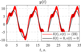
Figure 1: Behavior of $y\left(t\right)$ when $\delta\left(t\right){\rm{,\;}}v\left(t\right){\rm{:}}=0$ and $\delta\left(t\right){\rm{,\;}}v\left(t\right){\rm{:}}=\eqref{eq25}$.

Figure 1 illustrates that the chosen perturbations (23) noticeably affected the measured output of the system.

Figure 2a shows the behavior of the unknown parameter estimates when the laws (20), (26), (27) were applied. Figure 2b presents a comparison of $\hat{\theta}\left(t\right)$ transients for (20) using different values of the parameter $T$.

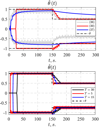
Figure 2: Behavior of a) $\hat{\theta}\left(t\right)$ for (20), (26), (27) and b) $\hat{\theta}\left(t\right)$ for (20) using different $T$ values.

The obtained transients of estimates $\hat{\theta}\left(t\right)$ allow one to make the following conclusions. The parametric error $\tilde{\theta}\left(t\right)$ using (26), (27) remained a bounded value and did not converge to zero even at $t\to\infty$. The proposed law (20) provided asymptotic convergence of the error $\tilde{\theta}\left(t\right)$ to an arbitrarily small neighborhood of zero defined by the parameter $T$.

V Conclusion

The dynamic regressor extension and mixing (DREM) procedure [3, 7] allows one to reduce most problems of adaptive control theory to the identification problem of parameters of a regression equation with a scalar regressor. However, in case of perturbations in the system/parameterization, in general, only biased estimates can be obtained asymptotically from this equation. In this study, based on the bias-eliminated least-squares (BELS) approach [22, 23], a modification of the DREM procedure is proposed to ensure asymptotic convergence of the parametric error to an arbitrarily small neighborhood of zero defined by the arbitrary parameter $T$. To ensure convergence of the obtained estimates, independence of at least one known element of the regressor from the perturbation (C2) and the fulfillment of the conditions (C1 and C3), similar to the well-known requirement of the regressor persistent excitation, are required.

The scope of further research is to apply the proposed estimation law to the problems of design of adaptive observers and composite adaptive control systems. Moreover, it also includes an investigation of the possibility to relax the conditions C1 and C3.

Appendix

Proof of Theorem 1. The regressor $\Delta\left(t\right)$ is defined as follows:

$$\Delta\left(t\right)={\rm{det}}\left\{{{\textstyle{1\over T}}\int\limits_{{\rm{max}}\left\{{{t_{0}}{\rm{,\;}}t-T}\right\}}^{t}{\phi\left(s\right){\phi^{\top}}\left(s\right)ds}}\right\}{\rm{,}}$$ (A1)

then, owing to the property (14) and continuity of the regressor $\Delta\left(t\right)$, for all $t\in\left[{{t_{0}}{\rm{,\;}}{T_{f}}}\right)$ the following conditions are considered to be met:

$$\Delta\left(t\right){\Delta^{-1}}\left(t\right)=0{\rm{,\;}}\dot{\Delta}\left(t\right)=0.$$ (A2)

For all $t\geq{T_{f}}$ as C1 is met, we have

$$\Delta\left(t\right)\geq{\underline{\alpha}^{2n}}>0$$ (A3)

and, consequently, the following error is well defined:

$$\tilde{\kappa}\left(t\right)=\hat{\kappa}\left(t\right)-{\Delta^{-1}}\left(t\right){\rm{,}}$$

which is differentiated with respect to time and, owing to

$$\begin{array}[]{c}\Delta\left(t\right){\Delta^{-1}}\left(t\right)=1\Leftrightarrow\dot{\Delta}\left(t\right){\Delta^{-1}}\left(t\right)+\Delta\left(t\right){\textstyle{{d{\Delta^{-1}}\left(t\right)}\over{dt}}}=0{\rm{,}}\\ \Updownarrow\\ {\textstyle{{d{\Delta^{-1}}\left(t\right)}\over{dt}}}=-\dot{\Delta}\left(t\right){\Delta^{-2}}\left(t\right){\rm{,}}\end{array}$$

it is obtained:

$$\begin{array}[]{l}\dot{\tilde{\kappa}}=-\gamma\Delta\left({\Delta\hat{\kappa}-1}\right)-\dot{\Delta}{{\hat{\kappa}}^{2}}+\dot{\Delta}{\Delta^{-2}}=\\ =-\gamma{\Delta^{2}}\tilde{\kappa}-\dot{\Delta}\left({\hat{\kappa}+{\Delta^{-1}}}\right)\tilde{\kappa}=\\ =-\left({\gamma{\Delta^{2}}+\dot{\Delta}\hat{\kappa}+\dot{\Delta}{\Delta^{-1}}}\right)\tilde{\kappa}{\rm{,}}\end{array}$$ (A4)

where $\dot{\Delta}\left(t\right)$ obeys Jacobi’s formula:

$$\dot{\Delta}\left(t\right)={\rm{tr}}\left({{\rm{adj}}\left\{{\Phi\left(t\right)}\right\}\dot{\Phi}\left(t\right)}\right){\rm{,\;}}\Delta\left({{t_{0}}}\right)=0.$$

The quadratic form $V\left(t\right)={\textstyle{1\over 2}}{\tilde{\kappa}^{2}}\left(t\right)$ is introduced, which derivative is written as:

$$\dot{V}\left(t\right)=-2\left({\gamma{\Delta^{2}}\left(t\right)+\dot{\Delta}\left(t\right)\hat{\kappa}\left(t\right)+\dot{\Delta}\left(t\right){\Delta^{-1}}\left(t\right)}\right)V\left(t\right){\rm{,}}$$

from which, when $\gamma{\Delta^{3}}\left(t\right)+\Delta\left(t\right)\dot{\Delta}\left(t\right)\hat{\kappa}\left(t\right)+\dot{\Delta}\left(t\right)\geq\eta\Delta\left(t\right)>0\;\forall t\geq{T_{f}}$, then for all $t\geq{T_{f}}$ there exists the following upper bound:

$$\left|{\tilde{\kappa}\left(t\right)}\right|\leq{e^{-\eta\left({t-{T_{f}}}\right)}}\left|{\tilde{\kappa}\left({{t_{0}}}\right)}\right|.$$ (A5)

For all $t\geq{T_{f}}\;$ $\hat{\theta}\left(t\right)$ is rewritten in the following form:

$$\begin{array}[]{l}\hat{\theta}\left(t\right)=\hat{\kappa}\left(t\right){{\cal L}_{0}}{\cal Y}\left(t\right)\pm{\Delta^{-1}}\left(t\right){{\cal L}_{0}}{\cal Y}\left(t\right)=\\ ={\Delta^{-1}}\left(t\right){{\cal L}_{0}}{\cal Y}\left(t\right)+\tilde{\kappa}\left(t\right){{\cal L}_{0}}{\cal Y}\left(t\right)=\\ =\theta+{\Delta^{-1}}\left(t\right){{\cal L}_{0}}{{\cal W}_{2}}\left(t\right)+\tilde{\kappa}\left(t\right){{\cal L}_{0}}{\cal Y}\left(t\right)=\\ =\theta+{\Delta^{-1}}\left(t\right){{\cal L}_{0}}{\rm{adj}}\left\{{\Phi\left(t\right)}\right\}{{\cal L}_{2}}{\cal L}_{2}^{\top}W\left(t\right)+\tilde{\kappa}\left(t\right){{\cal L}_{0}}{\cal Y}\left(t\right)=\\ =\theta+{{\cal L}_{0}}{\Phi^{-1}}\left(t\right)W\left(t\right)+\tilde{\kappa}\left(t\right){{\cal L}_{0}}{\cal Y}\left(t\right).\end{array}$$ (A6)

When C1 is met, for all $t\geq{T_{f}}$ it holds that

$${\Phi^{-1}}\left(t\right)={\left[{{\textstyle{1\over T}}\int\limits_{t-T}^{t}{\phi\left(s\right){\phi^{\top}}\left(s\right)ds}}\right]^{-1}}\geq{\overline{\alpha}^{-1}}{I_{2n}}{\rm{,}}$$ (A7)

and consequently, from (A6) we have the following upper bound of the error $\tilde{\theta}\left(t\right)$:

$$\begin{array}[]{l}\left\|{\tilde{\theta}\left(t\right)}\right\|\!\leq\!\left\|{{\Phi^{-1}}\left(t\right)}\right\|\left\|{{\textstyle{1\over T}}\int\limits_{t-T}^{t}{\phi\left(s\right)f\left(s\right)ds}}\right\|\!+\!\left|{\tilde{\kappa}\left(t\right)}\right|\left\|{{\cal Y}\left(t\right)}\right\|\\ \leq{\underline{\alpha}^{-1}}\left\|{{\textstyle{1\over T}}\int\limits_{t-T}^{t}{\phi\left(s\right)f\left(s\right)ds}}\right\|+{e^{-\eta\left({t-{T_{f}}}\right)}}\left|{\tilde{\kappa}\left({{t_{0}}}\right)}\right|\left\|{{\cal Y}\left(t\right)}\right\|{\rm{,}}\end{array}$$

from which, as $\left\|{{\cal Y}\left(t\right)}\right\|$ is bounded, for bounded $\varphi\left(t\right){\rm{,\;}}w\left(t\right)$ it is obtained:

$$\begin{array}[]{l}\mathop{{\rm{lim}}}\limits_{t\to\infty}\left\|{\tilde{\theta}\left(t\right)}\right\|\leq{\underline{\alpha}^{-1}}\left\|{\mathop{{\rm{lim}}}\limits_{t\to\infty}{\textstyle{1\over T}}\int\limits_{t-T}^{t}{\phi\left(s\right)f\left(s\right)ds}}\right\|{\rm{:}}=\varepsilon\left(T\right){\rm{,}}\\ \mathop{{\rm{lim}}}\limits_{T\to\infty}\varepsilon\left(T\right)={\underline{\alpha}^{-1}}\left\|{\mathop{{\rm{lim}}}\limits_{t\to\infty}\mathop{{\rm{lim}}}\limits_{T\to\infty}{\textstyle{1\over T}}\int\limits_{t-T}^{t}{\phi\left(s\right)f\left(s\right)ds}}\right\|=0{\rm{,}}\end{array}$$

which was to be proved.

Proof of theorem 2. The regressor $\omega\left(t\right)$ is defined as:

$$\begin{array}[]{l}\omega\left(t\right)\!=\!{\rm{det}}\!\left\{{{\textstyle{k\over{s+k}}}\!\left\{{{\rm{det}}\!\left\{{{{\cal H}^{\top}}\!{\rm{adj}}\left\{{\Phi\left(t\right)}\right\}\!{{\cal L}_{1}}}\right\}\Phi\left(t\right)}\right\}}\right\}\!{\rm{,}}\\ \Phi\left(t\right)={\textstyle{1\over T}}\int\limits_{{\rm{max}}\left\{{{t_{0}}{\rm{,\;}}t-T}\right\}}^{t}{\phi\left(s\right){\phi^{\top}}\left(s\right)ds}{\rm{,}}\end{array}$$ (A8)

then, owing to the property (14) and continuity of the regressor $\Delta\left(t\right)$, for all $t\in\left[{{t_{0}}{\rm{,\;}}{T_{f}}}\right)$ the following conditions are considered to be met:

$$\omega\left(t\right){\omega^{-1}}\left(t\right)=0{\rm{,\;}}\dot{\omega}\left(t\right)=0.$$ (A9)

For all $t\geq{T_{f}}$ as C1 and C3 are met, we have

$$\begin{array}[]{l}\overline{\alpha}{I_{2n}}\geq\Phi\left(t\right)\geq\underline{\alpha}{I_{2n}}>{\rm{0,}}\\ \overline{\beta}\geq\left|{{\rm{det}}\left\{{{{\cal H}^{\top}}{\rm{adj}}\left\{{\Phi\left(t\right)}\right\}{{\cal L}_{1}}}\right\}}\right|\geq\underline{\beta}>0\end{array}$$ (A10)

and, consequently, there exists ${\overline{T}_{f}}\geq{T_{f}}$ such that

$${\left({\overline{\alpha}\overline{\beta}}\right)^{2n}}\geq\left|{\omega\left(t\right)}\right|\geq{\left({\underline{\alpha}\underline{\beta}}\right)^{2n}}>{\rm{0,\;}}\forall t\geq{\overline{T}_{f}}.$$ (A11)

So, taking into consideration (A11), the following error is well defined for all $t\geq{\overline{T}_{f}}$:

$$\tilde{\kappa}\left(t\right)=\hat{\kappa}\left(t\right)-{\omega^{-1}}\left(t\right){\rm{,}}$$

which is differentiated with respect to time and owing to

$$\begin{array}[]{c}\omega\left(t\right){\omega^{-1}}\left(t\right)=1\Leftrightarrow\dot{\omega}\left(t\right){\omega^{-1}}\left(t\right)+\omega\left(t\right){\textstyle{{d{\omega^{-1}}\left(t\right)}\over{dt}}}=0\\ \Updownarrow\\ {\textstyle{{d{\omega^{-1}}\left(t\right)}\over{dt}}}=-\dot{\omega}\left(t\right){\omega^{-2}}\left(t\right),\end{array}$$

it is obtained:

$$\begin{array}[]{l}\dot{\tilde{\kappa}}=-\gamma\omega\left({\omega\hat{\kappa}-1}\right)-\dot{\omega}{{\hat{\kappa}}^{2}}+\dot{\omega}{\omega^{-2}}=\\ =-\gamma{\omega^{2}}\tilde{\kappa}-\dot{\omega}\left({\hat{\kappa}+{\omega^{-1}}}\right)\tilde{\kappa}=\\ =-\left({\gamma{\omega^{2}}+\dot{\omega}\hat{\kappa}+\dot{\omega}{\omega^{-1}}}\right)\tilde{\kappa}{\rm{.}}\end{array}$$ (A12)

The quadratic form $V\left(t\right)={\textstyle{1\over 2}}{\tilde{\kappa}^{2}}\left(t\right)$ is introduced, which derivative is written as:

$$\dot{V}\left(t\right)=-2\left({\gamma{\omega^{2}}\left(t\right)+\dot{\omega}\left(t\right)\hat{\kappa}\left(t\right)+\dot{\omega}\left(t\right){\omega^{-1}}\left(t\right)}\right)V\left(t\right){\rm{,}}$$

from which, when $\gamma{\omega^{3}}\left(t\right)+\omega\left(t\right)\dot{\omega}\left(t\right)\hat{\kappa}\left(t\right)+\dot{\omega}\left(t\right)\geq\eta\omega\left(t\right)>0\;\forall t\geq{\overline{T}_{f}}$, then for all $t\geq{\overline{T}_{f}}$ there exists the following upper bound:

$$\left|{\tilde{\kappa}\left(t\right)}\right|\leq{e^{-\eta\left({t-{{\overline{T}}_{f}}}\right)}}\left|{\tilde{\kappa}\left({{t_{0}}}\right)}\right|.$$ (A13)

For all $t\geq{\overline{T}_{f}}\;$ $\hat{\theta}\left(t\right)$ is rewritten in the following form:

$$\begin{gathered}\hat{\theta}\left(t\right)=\hat{\kappa}\left(t\right){\mathcal{L}_{0}}\Lambda\left(t\right)\pm{\omega^{-1}}\left(t\right){\mathcal{L}_{0}}\Lambda\left(t\right)=\hfill\\ ={\omega^{-1}}\left(t\right){\mathcal{L}_{0}}\Lambda\left(t\right)+\tilde{\kappa}\left(t\right){\mathcal{L}_{0}}\Lambda\left(t\right)=\hfill\\ =\theta+{\omega^{-1}}\left(t\right){\mathcal{L}_{0}}{\text{adj}}\left\{{{\Omega_{f}}}\right\}\tfrac{k}{{s+k}}\left\{\left[\mathcal{M}\left(t\right){\mathcal{L}_{2}}-\right.\right.\\ \left.\left.-{\mathcal{L}_{1}}{\text{adj}}\left\{{{\mathcal{H}^{\top}}{\text{adj}}\left\{{\Phi\left(t\right)}\right\}{\mathcal{L}_{1}}}\right\}{\mathcal{H}^{\top}}{\text{adj}}\left\{{\Phi\left(t\right)}\right\}{\mathcal{L}_{2}}\right]\times\right.\\ \left.\times\mathcal{L}_{2}^{\top}W\left(t\right)\right\}+\tilde{\kappa}\left(t\right){\mathcal{L}_{0}}\Lambda\left(t\right).\hfill\\ \end{gathered}$$ (A14)

When C1 and C3 are met, then, according to (A10), for all $t\geq{\overline{T}_{f}}$ it holds that:

$$0<\left|{{\omega^{-1}}\left(t\right)}\right|\leq{\left({\underline{\alpha}\underline{\beta}}\right)^{-2n}}{\rm{,\;adj}}\left\{{{\Omega_{f}}}\right\}\leq{\left({\overline{\alpha}\overline{\beta}}\right)^{2n-1}}{I_{2n}}{\rm{,}}$$

and consequently, from (A14) we have the following upper bound of the error $\tilde{\theta}\left(t\right)$:

$$\begin{gathered}\left\|{\tilde{\theta}\left(t\right)}\right\|\leqslant{\left({\underline{\alpha}\underline{\beta}}\right)^{-2n}}{\left({\overline{\alpha}\overline{\beta}}\right)^{2n-1}}\left\|\tfrac{k}{{s+k}}\left\{\left[\mathcal{M}\left(t\right){\mathcal{L}_{2}}-\right.\right.\right.\\ \left.\left.\left.-{\mathcal{L}_{1}}{\text{adj}}\left\{{{\mathcal{H}^{\top}}{\text{adj}}\left\{{\Phi\left(t\right)}\right\}{\mathcal{L}_{1}}}\right\}{\mathcal{H}^{\top}}{\text{adj}}\left\{{\Phi\left(t\right)}\right\}{\mathcal{L}_{2}}\right]\times\right.\right.\\ \left.\left.\times\mathcal{L}_{2}^{\top}W\left(t\right)\right\}\right\|+{e^{-\eta\left({t-{{\overline{T}}_{f}}}\right)}}\left|{\tilde{\kappa}\left({{t_{0}}}\right)}\right|\left\|{\Lambda\left(t\right)}\right\|.\hfill\\ \end{gathered}$$ (A15)

When C2 is met, then, following (11), it holds that:

$$\mathop{{\rm{lim}}}\limits_{T\to\infty}{\cal L}_{2}^{\top}W\left(t\right)\!=\!\mathop{{\rm{lim}}}\limits_{T\to\infty}{\textstyle{1\over T}}{\cal L}_{2}^{\top}\int\limits_{{\rm{max}}\left\{{{t_{0}}{\rm{,\;}}t-T}\right\}}^{t}{\!\!\!\!\phi\left(s\right)f\left(s\right)ds}=0$$

from which, as $\Lambda\left(t\right)$ and $\mathcal{M}\left(t\right){\mathcal{L}_{2}}-{\mathcal{L}_{1}}{\text{adj}}\left\{{{\mathcal{H}^{\top}}{\text{adj}}\left\{{\Phi\left(t\right)}\right\}{\mathcal{L}_{1}}}\right\}{\mathcal{H}^{\top}}{\text{adj}}\left\{{\Phi\left(t\right)}\right\}{\mathcal{L}_{2}}$ are bounded, for bounded $\varphi\left(t\right){\rm{,\;}}w\left(t\right)$ and any $T>0$ there exists $c>0$ such that:

$$\begin{gathered}\mathop{{\text{lim}}}\limits_{t\to\infty}\left\|{\tilde{\theta}\left(t\right)}\right\|\leqslant{\left({\underline{\alpha}\underline{\beta}}\right)^{-2n}}{\left({\overline{\alpha}\overline{\beta}}\right)^{2n-1}}\left\|\tfrac{k}{{s+k}}\left\{\left[\mathcal{M}\left(t\right){\mathcal{L}_{2}}-\right.\right.\right.\\ \left.\left.\left.-{\mathcal{L}_{1}}{\text{adj}}\left\{\!{{\mathcal{H}^{\top}}{\text{adj}}\left\{\!{\Phi\left(t\right)}\!\right\}{\mathcal{L}_{1}}}\!\right\}\!{\mathcal{H}^{\top}}\!{\text{adj}}\left\{\!{\Phi\left(t\right)}\!\right\}{\mathcal{L}_{2}}\right]\mathcal{L}_{2}^{\top}W\left(t\right)\right\}\right\|\leqslant\hfill\\ \leqslant c\left\|{\mathop{{\text{lim}}}\limits_{t\to\infty}\tfrac{k}{{s+k}}\left\{{\mathcal{L}_{2}^{\top}W\left(t\right)}\right\}}\right\|{\text{:}}=\varepsilon\left(T\right){\text{,}}\hfill\\ \mathop{{\text{lim}}}\limits_{T\to\infty}\varepsilon\left(T\right)=c\left\|{\mathop{{\text{lim}}}\limits_{t\to\infty}\mathop{{\text{lim}}}\limits_{T\to\infty}\tfrac{k}{{s+k}}\left\{{\mathcal{L}_{2}^{\top}W\left(t\right)}\right\}}\right\|=\hfill\\ =c\left\|{\mathop{{\text{lim}}}\limits_{t\to\infty}\tfrac{k}{{s+k}}\left\{{\mathop{{\text{lim}}}\limits_{T\to\infty}\mathcal{L}_{2}^{\top}W\left(t\right)}\right\}}\right\|=0{\text{,}}\hfill\\ \end{gathered}$$

which was to be proved.

References

[1] Kreisselmeier G., “Adaptive observers with exponential rate of convergence,” IEEE Transactions on Automatic Control, vol. 22, no.1, pp. 2–8, 1977.
[2] Kreisselmeier G., “On adaptive state regulation,” IEEE Transactions on Automatic Control, vol. 27, no. 1, pp. 3–17, 1982.
[3] Aranovskiy, S., Bobtsov, A., Ortega, R., Pyrkin, A., “Parameters estimation via dynamic regressor extension and mixing,” Proceedings of the 2016 American Control Conference, pp. 6971–6976, 2016.
[4] de Mathelin M., Lozano R., “Robust adaptive identification of slowly time-varying parameters with bounded disturbances,” Automatica, vol.35, no. 7, pp. 1291-1305, 1999.
[5] Lion P. M., “Rapid identification of linear and nonlinear systems,” AIAA Journal, vol. 5, no. 10, pp. 1835–1842, 1967.
[6] Wang L., Ortega R., Bobtsov A., Romero J. G., Yi B., “Identifiability implies robust, globally exponentially convergent on-line parameter estimation,” International Journal of Control, pp. 1–17, 2023. Early access.
[7] Ortega R., Nikiforov V., Gerasimov D., “On modified parameter estimators for identification and adaptive control. A unified framework and some new schemes,” Annual Reviews in Control, vol. 50, pp. 278–293, 2020.
[8] Ortega R., Romero J. G., Aranovskiy S., “A new least squares parameter estimator for nonlinear regression equations with relaxed excitation conditions and forgetting factor,” Systems & Control Letters, vol. 169, pp. 105377, 2022.
[9] Korotina M., Romero J. G., Aranovskiy S., Bobtsov A., Ortega R., “A new on-line exponential parameter estimator without persistent excitation,” Systems & Control Letters, vol. 159, pp. 105079, 2022.
[10] Ortega R., Aranovskiy S., Pyrkin A. A., Astolfi A., Bobtsov A. A., “New results on parameter estimation via dynamic regressor extension and mixing: Continuous and discrete-time cases,” IEEE Transactions on Automatic Control, vol. 66, no. 5, pp. 2265–2272, 2020.
[11] Wang J., Efimov D., Bobtsov A., “On robust parameter estimation
in finite-time without persistence of excitation,” IEEE Transactions on Automatic Control, vol. 65, no. 4, pp. 1731–1738, 2019.
[12] Wang J., Efimov D., Aranovskiy S., Bobtsov A., “Fixed-time estimation of parameters for non-persistent excitation,” European Journal of Control, vol. 55, no. 4, pp. 24–32, 2020.
[13] Korotina M., Aranovskiy S., Ushirobira R., Vedyakov, A., “On parameter tuning and convergence properties of the DREM procedure,” Proceedings of the 2020 European Control Conference (ECC), pp. 53–58, 2020.
[14] Aranovskiy S., Ushirobira R., Korotina M., Vedyakov A., “On preserving-excitation properties of Kreisselmeier’s regressor extension scheme,” IEEE Transactions on Automatic Control, vol. 68, no. 2., pp.1296–1302, 2022.
[15] Yi B., Ortega R., “Conditions for convergence of dynamic regressor extension and mixing parameter estimators using LTI filters,” IEEE Transactions on Automatic Control, vol. 68, no. 2., pp.1253–1258, 2022.
[16] Aranovskiy S., Bobtsov A. A., Pyrkin A. A., Ortega R., Chaillet A., “Flux and position observer of permanent magnet synchronous motors with relaxed persistency of excitation conditions,” IFAC-PapersOnLine, vol. 48, no. 11, pp. 301–306, 2015.
[17] Glushchenko A., Lastochkin K., “Exact Asymptotic Estimation of Unknown Parameters of Perturbed LRE with Application to State Observation,” arXiv preprint arXiv:2310.14073. pp.1–6, 2024.
[18] Korotina M., Aranovskiy S., Ushirobira R., Efimov D., Wang J., “Fixed-time parameter estimation via the discrete-time drem method,” IFAC-PapersOnLine, vol.56, no.2, pp. 4013–4018, 2023.
[19] Vorobyev V., Bobtsov A., Nikolaev N., Pyrkin A., “Application of a nonlinear operator to identify an unknown parameter for a scalar regression equation with disturbance in the measurement channel,” arXiv preprint arXiv:2305.16359. pp.1–9, 2023.
[20] Bobtsov A., Vorobyev V., Nikolaev N., Pyrkin A., Ortega R., “Synthesis of an adaptive observer of state variables for a linear stationary object in the presence of measurement noise,” arXiv preprint arXiv:2305.15496. pp.1–14, 2023.
[21] Glushchenko A., Lastochkin K., “Instrumental Variables based DREM for Online Asymptotic Identification of Perturbed Linear Systems,” arXiv preprint arXiv:2312.15631. pp.1–13, 2023.
[22] Zheng W. X., Feng C. B., “A bias-correction method for indirect identification of closed-loop systems,” Automatica, vol.31, no. 7, pp. 1019-1024, 1995.
[23] Gilson M., Van den Hof P., “On the relation between a bias-eliminated least-squares (BELS) and an IV estimator in closed-loop identification,” Automatica, vol.37, no. 10, pp. 1593-1600, 2001.