Efficient Diffusion-Driven Corruption Editor
for Test-Time Adaptation

Abstract

Test-time adaptation (TTA) addresses the unforeseen distribution shifts occurring during test time. In TTA, both performance and, memory and time consumption serve as crucial considerations. A recent diffusion-based TTA approach for restoring corrupted images involves image-level updates. However, using pixel space diffusion significantly increases resource requirements compared to conventional model updating TTA approaches, revealing limitations as a TTA method. To address this, we propose a novel TTA method by leveraging a latent diffusion model (LDM) based image editing model and fine-tuning it with our newly introduced corruption modeling scheme. This scheme enhances the robustness of the diffusion model against distribution shifts by creating (clean, corrupted) image pairs and fine-tuning the model to edit corrupted images into clean ones. Moreover, we introduce a distilled variant to accelerate the model for corruption editing using only 4 network function evaluations (NFEs). We extensively validated our method across various architectures and datasets including image and video domains. Our model achieves the best performance with a 100 times faster runtime than that of a diffusion-based baseline. Furthermore, it outpaces the speed of the model updating TTA method based on data augmentation threefold, rendering an image-level updating approach more practical.

1 Introduction

Test-time adaptation (TTA) [59] is a task aimed at achieving higher performance than simple inference when there is a distribution shift between source and target domain, using a minimal resource (e.g., inference time and memory consumption) overhead. Traditional TTA methodologies [59, 44, 43, 3] primarily update only a subset of model parameters or manipulate the model’s output to obtain predictions adapted to the target distribution. However, these methodologies show sensitive performance under wild scenarios [44, 27] (e.g., biased, label shifts, mixed, and batch size $1$ scenarios) and episodic setting [61].

Gao et al. [13] first proposed a diffusion-based image-level (input) updating approach for TTA called diffusion-driven adaptation (DDA), which restores the input image via an ImageNet [10] pre-trained pixel-space diffusion model [11]. DDA shows more robust performance than model-updating TTA approaches [59, 67] under episodic settings and consistent performance enhancement with various architectures. However, the backbone diffusion model, DDPM [18], requires large memory consumption and a significant amount of inference time. Given the resource and time constraints inherent in TTA, implementing DDA in real-world applications is not feasible. Therefore, for the effective usability of an image-level updating TTA, it is essential to incorporate fast and lightweight input updates.

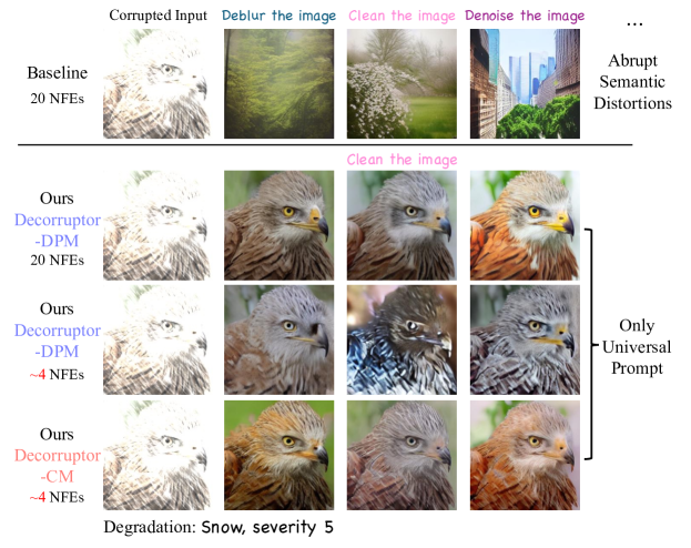
Figure 1: Visualization of instruction-guided image editing for the unseen corrupted image at the test-time. Compared to the baseline IP2P method, our proposed Decorruptor-DPM ($20$-step) and Decorruptor-CM ($4$-step) models show effective editing results without hurting the original semantics of the input corrupted image.

To achieve efficient adaptation, we consider using Instruct-Pix2Pix (IP2P) [4], a method that utilizes a latent diffusion model (LDM) [47]. IP2P takes both text instructions and images as conditions to enable instruction-based image editing. This approach leverages not pixel space but latent space, which facilitates the efficient generation of images. However, as shown in the first row of Fig. 1, IP2P model is infeasible for TTA scenarios where out-of-domain (i.e., corrupted) images become inputs, as it can only edit in-domain images into in-domain images. Thus, to utilize IP2P model in TTA scenarios, it is crucial to enhance its robustness under distribution shifts, including test-time corruption.

In this paper, we propose a new diffusion-based input updating TTA methodology named Decorruptor using diffusion probabilistic model (Decorruptor-DPM) that can efficiently respond to unseen corruptions. To enhance the diffusion model’s robustness, we draw inspiration from data augmentation methods [9, 65, 64, 16], known for their efficacy in enhancing robustness against distribution shifts. In response, Decorruptor-DPM applies a novel corruption modeling scheme to IP2P: generate (clean, corrupted) image pairs and use them for fine-tuning to facilitate the restoration of corrupted images to their clean counterparts. To the best of our knowledge, the application of data augmentation for enhancing the robustness of the diffusion model appears to be unexplored in existing literature. Decorruptor-DPM supports efficient editing against test-time corruption as can be seen in Fig. 1, requiring only a universal instruction. In addition, Decorruptor-DPM enables 46 times faster input updates than DDA owing to the latent-level computation and fewer generation steps. To be practically applicable with TTA, where inference time is crucial, we further propose Decorruptor using consistency model (Decorruptor-CM), the accelerated variant of Decorruptor-DPM, by distilling the diffusion using consistency distillation [37]. As shown in Fig. 1, Decorruptor-CM achieves similar corruption editing effects to Decorruptor-DPM’s 20 network function evaluations (NFEs) with only 4 NFEs.

We assess the performance of data edited by our models on the ImageNet-C [15] and ImageNet-$\bar{\mathrm{C}}$ [39], with various architectures. With around 100 times faster runtime, our models exhibited the best performance on ImageNet-C and -$\bar{\mathrm{C}}$ across various architectures. Notably, Decorruptor-CM demonstrated superior performance compared to MEMO [67], an image augmentation-based model updating TTA method, achieving three times speed enhancements. Contrary to DDA, which shows a performance drop across certain architectures, our approach reveals improvements in all evaluated architectures. Additionally, by harnessing its rapid inference, Decorruptor-CM extends its applicability from the image to the video domain, showcasing outperforming editing outcomes on the UCF-101 [58] video dataset when compared to DDA. Our contributions are as follows:

• We propose Decorruptor-DPM that enhances the robustness and efficiency of diffusion-based input updating approach for TTA through the incorporation of a novel corruption modeling scheme within the LDM.

• We propose Decorruptor-CM, as an accelerated model, by distilling the DPM to significantly reduce inference time with minimal performance degradation. By ensembling multiple edited images’ predictions, Decorruptor-CM even achieves higher classification accuracy than Decorruptor-DPM while being faster in execution.

• We demonstrate high performance and generalization capabilities with a faster runtime through extensive experiments on image and video TTA. Decorruptor-CM shows three times faster runtime than MEMO, making an input updating approach more practical.

2 Related Works

2.1 Latent Diffusion Models

The latent diffusion model (LDM) [47] is a representative method that overcomes the large memory/time consumption drawbacks of DDPM [18]. LDM reduces memory consumption and inference time by performing the denoising process in latent space instead of pixel space. Stable diffusion (SD) [47], a scaled-up version of LDM, is a large-scale pre-trained text-to-image diffusion model that has shown unprecedented success in high-quality and diverse image synthesis. Unlike previous SD-based image editing methodologies [17, 46] which require paired texts in the image editing stage, InstructPix2Pix [4] enables image editing solely based on instructions. However, as IP2P only supports clean input images, we enable corruption editing by fine-tuning the diffusion models with our proposed corruption modeling scheme.

2.2 Image Restoration

In the image restoration (IR) task, several works have been proposed to exploit the advantages of diffusion models. To solve linear inverse problems for IR tasks such as inpainting, denoising, deblurring, and super-resolution, applying SD [1, 8, 22] in image restoration has recently emerged. However, since SD relies on classifier-free guidance [19] with text-conditioning for image editing, a significant limitation exists to applying SD itself to TTA to remove arbitrary unseen test-time corruptions. To be specific, it is infeasible as previous text-guided image editing methods used for image restoration domain require prior knowledge of text information corresponding to the test-time corruption [1, 8, 22], or necessitates such as a blur kernel or other degradation matrices [7, 62, 24]. In this paper, we elucidate that our work is significantly different from IR tasks, as we do not require either pre-defined corruption information or degradation matrices for corruption editing at test time.

Table 1: Comparisons with multiple image-to-image tasks. IN indicates ImageNet. Our Decorruptor shows efficiency, generalizability, and high performance.

TTA requirements		Image Editing	Image Reconstruction		Image Decorruption
		InstructPix2Pix [4]	DDRM [25]	DPS [7]	DDA [13]	Ours (DPM / CM)
Efficiency (Minimal overhead)	NFEs	20	20	1000	50	20 / 4
	Noise space	Latent space	Pixel space	Pixel space	Pixel space	Latent space
Generalization	Degradation type	✗	Pre-defined	Pre-defined	Unseen	Unseen
Performance	IN-C Acc (%)	✗	✗	✗	29.7	30.5 / 32.8
	IN-$\bar{\mathrm{C}}$ Acc (%)	✗	✗	✗	29.4	41.8 / 47.1

2.3 Test-Time Adaptation

TTA aims to enhance inference performance with minimal resource overhead under distribution shifts. In contrast to unsupervised domain adaptation (UDA) [12, 49, 45], TTA lacks access to the source data. Moreover, unlike source-free domain adaptation [30, 28, 20], TTA has an online characteristic, obtaining target data only once through streaming. A prominent approach in TTA involves updating only a subset of parameters [59, 43, 44, 27]. However, model updating TTA methods face a risk of catastrophic forgetting [43, 61] as it lacks access to source data during training. Furthermore, the absence of clear criteria for hyperparameter selection poses a drawback, making it challenging to ensure performance in practical applications [69]. Gao et al. [13] presents diffusion-driven adaptation (DDA) to overcome these limitations. DDA utilizes a pre-trained diffusion model to transform corrupted input images into clean in-distribution images, updating the input images instead of the model. This approach enhances robustness in single-image evaluation as well as in ordered data scenarios. However, DDA falls short of meeting the efficiency requirement of TTA, as obtaining predictions for a single sample takes a long time. We greatly overcome such efficiency drawbacks. By combining LDM and CM, our model achieves higher performance and significantly reduced inference time compared to DDA. The overview of comparisons with related works are summarized in Table 1.

3 Preliminaries

3.1 Diffusion Models

Diffusion models [52, 18], also known as score-based generative models [56, 57], are popular family of generative models that generate data from Gaussian noise. Specifically, these models learn to reverse a diffusion process that translates the original data distribution $p_{\text{data}}(x)$ towards a marginal distribution $q_{t}(x_{t})$, facilitated by a transition kernel defined as $q_{0t}(x_{t}|x_{0})=\mathcal{N}(x_{t}|\alpha(t)x_{0},\sigma^{2}(t)I)$, in which $\alpha(t)$ and $\sigma(t)$ are pre-defined noise schedules. Viewed from a continuous-time perspective, this diffusion process can be modeled by a stochastic differential equation (SDE) [57, 23] over the time interval $[0,T]$. To learn the reverse of SDE, diffusion models are trained to estimate score function $\epsilon_{\theta}(z_{t},t)$ with U-Net architecture [48]. Song et al. [57] show that the reverse process of SDE has its corresponding probability flow original differential equation (PF-ODE).

3.1.1 Classifier Free Guidance

During inference, diffusion models use the classifier-free guidance (CFG) [19] to ensure the input conditions such as text and class labels. Compared to the classifier guidance [11] that requires training an additional classifier, the CFG operates without the need for a pre-trained classifier. Instead, CFG utilizes a linear combination of score estimates from an unconditional diffusion model trained concurrently with a conditional diffusion model:

$$\hat{\epsilon}_{\theta}(z_{t},\omega,t,c):=(1+\omega)\epsilon_{\theta}(z_{t},t,c)-\omega\epsilon_{\theta}(z_{t},t,\emptyset).$$ (1)

3.2 Consistency Models

The slow generation speed of diffusion models, due to their iterative updating nature, is a known limitation. To overcome this, the Consistency Model (CM) [55] has been introduced as a new generative model that accelerates generation to a single step or a few steps. CM operates on the principle of mapping any point from the trajectory of the PF-ODE to its destination. This is achieved through a consistency function defined as $f:(x_{t},t)\mapsto x_{\varepsilon}$, where $\varepsilon$ is a small positive value. A key aspect of CM is that the consistency function must fulfill the self-consistency property:

$$f(x_{t},t)=f(x_{t^{\prime}},t^{\prime}),\quad\forall t,t^{\prime}\in[\varepsilon,T].$$ (2)

To ensure that $f_{\theta}(x,\varepsilon)=x$, the consistency model $f_{\theta}$ can be parameterized as $f_{\theta}(x,t)=c_{\text{skip}}(t)x+c_{\text{out}}(t)F_{\theta}(x,t)$, where $c_{\text{skip}}(t)$ and $c_{\text{out}}(t)$ are differentiable functions with $c_{\text{skip}}(\varepsilon)=1$ and $c_{\text{out}}(\varepsilon)=0$, and $F_{\theta}(x,t)$ is a deep neural network and it becomes $(\mathbf{z}_{t}-\sigma_{t}\hat{\epsilon}(\mathbf{z},c,t))/{\alpha_{t}}$ for $\epsilon$-prediction models like Stable Diffusion. One way to train a consistency model is to distill a pre-trained diffusion model, by training an online model $\theta$ while updating target model $\theta^{-}$ with exponential moving average (EMA), defined as $\theta^{-}\leftarrow\mu\theta^{-}+(1-\mu)\theta$. The consistency distillation loss is defined as follows:

$$\mathcal{L}(\theta,\theta^{-};\Phi)=\mathbb{E}_{x_{t}}\left[d\left(f_{\theta}(x_{t_{n}},t_{n+1}),f_{\theta^{-}}\left(\hat{x}_{t_{n}},t_{n}\right)\right)\right],$$ (3)

where $d(\cdot,\cdot)$ is a squared $\ell_{2}$ distance $d(x,y)=\|x-y\|^{2}$, and $\hat{x}_{t_{n}}$ is a one-step estimation of $x_{t_{n}}$ from $x_{t_{n+1}}$ as $\hat{x}_{t_{n}}\leftarrow x_{t_{n+1}}+(t_{n}-t_{n+1})\Phi(x_{t_{n+1}},t_{n+1};\Phi)$, where $\Phi$ denotes the numerical ODE solver like DDIM [54].

Luo et al. [37] recently introduced Latent Consistency Models (LCM) which accelerate a text-to-image diffusion model. They propose a consistency function $f_{\theta}:(z_{t},\omega,c,t)\mapsto z_{0}$ that directly predicts the solution of PF-ODE augmented by CFG, with additional guidance scale condition $\omega$ and text condition $c$. The LCM is trained by minimizing the loss

$$\mathcal{L}_{LCD}(\theta,\theta^{-};\Psi)=\mathbb{E}_{z_{t},\omega,c,n}\left[d\left(f_{\theta}(z_{t_{n+1}},\omega,c,t_{n+1}),f_{\theta^{-}}(\hat{z}_{t_{n}}^{\Psi,\omega},\omega,c,t_{n})\right)\right].$$ (4)

Here, $\omega$ and $n$ are uniformly sampled from interval $[\omega_{\text{min}},\omega_{\text{max}}]$ and $[1,\ldots,N-1]$ respectively. $\hat{z}_{t_{n}}^{\Psi,\omega}$ is estimated using the pre-trained diffusion model and PF-ODE solver $\Psi$ [54], represented as follows:

$$\hat{z}_{t_{n}}^{\Psi,\omega}-z_{t_{n+1}}\approx(1+\omega)\Psi(z_{t_{n+1}},t_{n+1},t_{n},c)-\omega\Psi(z_{t_{n+1}},t_{n+1},t_{n},\emptyset).$$ (5)

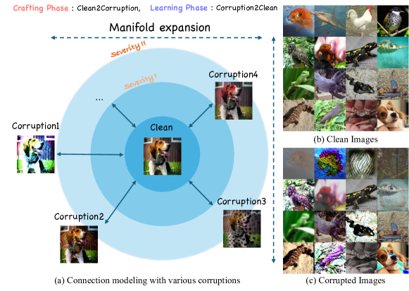
Figure 2: Representations of (a) Instance-wise connection map for corruption-like augmentations, corruption crafting results of (b) clean images to (c) corrupted images. In (a), we showcase how we constitute various corruption-like augmentations. Here, the sensitivity means the granularity of the corruption, the crafting phase means how to create the corrupted images, and the learning phase means how to learn editing.

4 Proposed Method

A crucial consideration of Decorruptor lies in the diversity of augmentations on corruption-like augmentations during the inductive learning stage. To this end, we elucidate how we get the paired data of clean and corrupted data in 4.1, fine-tuning the models using those pairs in 4.2, distilling the model for acceleration at inference time in 4.3, and explanations on overall process in 4.4.

4.1 Corruption Modeling Scheme

Data augmentation is being used across various fields to enhance robustness against distribution shifts, including supervised [65, 64], semi-supervised [53], and self-supervised learning [5]. Similarly, in TTA, MEMO [67] applies multiple data augmentations to a single input. Notably, it utilizes $64$ data augmentations on test-time input to minimize marginal entropy and enables more stable adaptation than TENT [59].

As shown in the first row of Fig. 1, the pre-trained diffusion model does not generalize well to out-of-domain data not used during training. Therefore, to effectively utilize diffusion in TTA with incoming unseen corrupted data, the diffusion model also needs robustness against corruption. To this end, as a method to impose the diffusion model with robustness, we introduce a novel corruption modeling scheme: create pairs of (clean, corrupted) images and utilize them for fine-tuning to enable the recovery of corrupted images to their clean states. Through the training process of editing corrupted images onto clean ones, we broaden the diffusion model’s manifold to edit corrupted inputs, enhancing robustness against unseen corruptions. To the best of our knowledge, this novel scheme to robustify the diffusion models has not been previously explored.

To create corrupted data, we employed prevalent data augmentation strategies on the given clean images. PIXMIX [16], for example, performs data augmentation in an on-the-fly manner based on class-agnostic complex images. Furthermore, we also consider the widely-used data augmentation method for self-supervised contrastive learning, such as SimSiam [5]. As described in Fig. 2 (a), for the crafting phase, the corrupted samples are easily crafted in a one-to-many manner from the clean image. In the following, for the learning phase, we utilized these corrupted samples for many-to-one training for corruption editing via our Decorruptor-DPM model with ‘Clean the image’ instruction $c_{T}$. Thus, our model is trained to restore mixed complex corruptions from the diverse augmented samples $c_{I}$ onto clean image $x$.

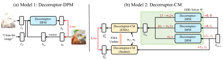
Figure 3: Schematic of the overall training pipeline for the two proposed model variants: (a) Decorruptor-DPM, (b) Decorruptor-CM.

4.2 Decorruptor-DPM: Instruction-Based Corruption Editing

To train our diffusion model, as it diffuses the image in the latent space, the training objective can be rewritten as the following equation:

$$\mathcal{L}(\theta)=\mathbb{E}_{z\sim\mathcal{E}(x),c_{T},\epsilon\sim\mathcal{N}(0,1),t}\left[\|\epsilon-\epsilon_{\theta}(\mathbf{z}_{t},t,c_{T},c_{I})\|^{2}\right],$$ (6)

where $x$ denotes an image, $z$ is the encoded latent, $z_{t}$ denotes diffused latents at timestep $t\in T$, text condition $c_{T}$, and corrupted image condition $c_{I}$.

4.2.1 Fine-Tuning U-Net With Corruption-Like Augmentations

We note that the large-scale LAION dataset [51], encompassing diverse image domains including art, 3D, and aesthetic categories, is highly different from the ImageNet dataset. Thus, exploiting the IP2P model itself, which is fine-tuned on generated samples with SD trained on the LAION dataset, inevitably generates domain-biased samples when using it for corruption editing of ImageNet data.

To overcome such limitations, we have fine-tuned the diffusion model’s U-Net [48] initialized from the checkpoint of SD [47] via IP2P training protocol on corrupted images using only ImageNet [10] training data, ensuring they can edit images with the universal prompt alone. We use the same prompt used at training time that can revert unknown corruptions at inference time. This distinguishes our approach from previous works that required significant effort for prompt engineering. To facilitate image conditioning, following Brooks et al. [4], we introduce extra input channels into the initial convolutional layer. The diffusion model’s existing weights are initialized using pre-trained checkpoints, while the weights associated with the newly incorporated input channels are set to zero. The illustration of our Decorruptor-DPM is represented in Fig. 3 (a).

4.2.2 Scheduling Image Guidance Scale

At inference time, for Decorruptor-DPM, we utilized 20 DDIM steps and modified the image guidance scheduling to enable more effective editing. Unlike the text guidance scale, the image guidance scale is a hyper-parameter that determines how much of the input semantics are retained. Considering multi-modal conditioning guidances of the input image $c_{I}$ and text instructions $c_{T}$, CFG for our Decorruptor-DPM is as follows:

$$\hat{\epsilon}_{\theta}(z_{t},t,c_{I},c_{T}) =\epsilon_{\theta}(z_{t},t,\emptyset,\emptyset)+\omega_{I}(t)(\epsilon_{\theta}(z_{t},t,c_{I},\emptyset)-\epsilon_{\theta}(z_{t},t,\emptyset,\emptyset))$$ (7)

$$+\omega_{T}(\epsilon_{\theta}(z_{t},t,c_{I},c_{T})-\epsilon_{\theta}(z_{t},t,c_{I},\emptyset)).$$

It is known that if the scale is too large, the image tends to remain almost unchanged during editing, and conversely, if it is too small, the original image semantics are ignored, relying solely on text guidance for editing [4]. Since our input image is corrupted, we notice that the large guidance scale is needed at the large timestep of the pure noise phase, and a smaller guidance scale is used at the near image phase. Thus, in Eq. 7, we employed sqrt-scheduling for the image guidance scale $s_{I}$ by sampling it from $1.8$ to $0$ for $t\in[T,0]$.

4.3 Decorruptor-CM: Accelerate DPM to CM

Motivated by consistency distillation introduced in Sec. 3.2, we train a distilled variant for faster inference. The visual representations of our Decorruptor-CM model are illustrated in Fig. 3 (b). Following the latent consistency distillation training protocol of LCM [37], we train Decorruptor-CM by minimizing the objective:

$$\mathcal{L}_{LCD}(\theta,\theta^{-};\Psi)=\mathbb{E}_{z_{t},\omega,n}\left[d\left(f_{\theta}(z_{t_{n+1}},\omega,c,t_{n+1}),f_{\theta^{-}}(\hat{z}_{t_{n}}^{\Psi,\omega_{I},\omega_{T}},\omega,c,t_{n})\right)\right],$$ (8)

where $f_{\theta}$ represents the student consistency model, $f_{\theta^{-}}$ denotes EMA of $f_{\theta}$, $\omega$ contains two guidance scales $\omega_{T}$ and $\omega_{I}$, and $c$ contains two conditions $c_{T}$ and $c_{I}$. EMA model’s input $\hat{z}_{t_{n}}^{\Psi,\omega_{I},\omega_{T}}$ is a prediction of the Decorruptor-DPM using PF-ODE solver augmented with multi-modal guidances:

$$\hat{z}_{t_{n}}^{\Psi,\omega_{I},\omega_{T}}-z_{t_{n+1}} \approx\Psi(z_{t_{n+1}},t_{n+1},t_{n},\emptyset,\emptyset)$$ (9)

$$+\omega_{I}(\Psi(z_{t_{n+1}},t_{n+1},t_{n},c_{I},\emptyset)-\Psi(z_{t_{n+1}},t_{n+1},t_{n},\emptyset,\emptyset))$$

$$+\omega_{T}(\Psi(z_{t_{n+1}},t_{n+1},t_{n},c_{I},c_{T})-\Psi(z_{t_{n+1}},t_{n+1},t_{n},c_{I},\emptyset)).$$

We train on the same dataset employed during the DPM training phase. While previous work [37] has only augmented PF-ODE with text guidance, we introduce augmentation with multi-modal guidance as described in Eq. 9. Multi-modal guidance has not been previously explored for diffusion distillation.

In integrating the CFG scales $\omega_{T}$ and $\omega_{I}$ into the LCM, we employ Fourier embedding for both scales, following conditioning mechanisms of previous works [37, 38]. We use the zero-parameter initialization [66] for stable training. We sample the embeddings $w_{I}$ and $w_{T}$, with a dimension of $768$, and multiply each other for U-Net conditioning. This approach allows the two variables to act as independent conditions during training, facilitating the multi-modal conditionings. Following Luo et al. [37], $\omega_{T}^{\text{min}}$ and $\omega_{T}^{\text{max}}$ are set to $5.0$ and $15.0$, and we set $\omega_{I}^{\text{min}}$ and $\omega_{I}^{\text{max}}$ to be $1.0$ and $1.5$, respectively. It is worth noting that, unlike DPM, the integration of a learnable guidance scale obviates the need for image guidance scale scheduling.

4.4 Overall Process

The overall process for our efficient input updating TTA is as follows. First, complete the training of Decorruptor before TTA. Next, upon receiving the input image $x_{0}$, obtain the edited image $\hat{x}_{0}$ through Decorruptor. Finally, following the protocol of Gao et al. [13], perform an ensemble to obtain the final prediction to capitalize on the classifier’s knowledge from the target domain. It simply averages two predictions of $x_{0}$ and $\hat{x}_{0}$:

$$y^{pred}=0.5*(p_{\phi}(y|x_{0})+p_{\phi}(y|\hat{x}_{0})),$$ (10)

where $y^{pred}$ means the final prediction of our TTA method and $p_{\phi}(x)$ means the probabilistic prediction of input $x$ by the pre-trained classifier $p_{\phi}$. In contrast to Gao et al., we utilize probabilistic output after the softmax layer rather than logits for ensembling.

5 Experimental Results

In this section, we quantitatively and qualitatively validate Decorruptor. Through further analyses, we compare Decorruptor with the baseline in various aspects and demonstrate Decorruptor’s extensibility to other tasks.

5.1 Setup

5.1.1 Benchmarks

ImageNet-C [15] is a benchmark dataset generated by applying a total of 15 algorithmically generated corruptions, categorized into four groups: noise, blur, weather, and digital, to the ImageNet [10] dataset. It is utilized for evaluating the robustness under distribution shift and serves as a benchmark dataset in various tasks such as TTA and UDA. ImageNet-$\bar{\mathrm{C}}$ [39] comprises 10 corruptions that are perceptually dissimilar to those in ImageNet-C in the feature space. Additionally, to assess the effectiveness of our method in the video domain, we use UCF101-C [32], a benchmark dataset incorporating corruptions into UCF101 [58], which has a different distribution from the ImageNet.

5.1.2 Baselines

For comparison, we utilized three baselines that are not influenced by the compositions (e.g., label shifts, and batch size). DiffPure [42] is a method that employs diffusion for adversarial defense. DDA [13] uses a method that injects noise and then denoises using an in-domain pre-trained DDPM. Inspired by ILVR [6], DDA provides input that has passed through a low-pass filter as guidance and prevents catastrophic forgetting through self-ensembling. MEMO [67] is a model updating TTA approach that applies multiple data augmentations to a single input. Here, MEMO applies data augmentation to the input and tunes the classifier by minimizing the averaged prediction over augmentations. In contrast, Decorruptor uses augmentation when tuning the diffusion model for robustness against distribution shifts before adaptation.

5.1.3 Architectures

We conducted the evaluation using ResNet50 [14], the most standard and lightweight network. Subsequently, to assess consistent performance improvement across various architectures, we followed the protocol of the Gao et al. [13]: evaluating methods using the advanced forms of transformer structures (Swin-T, B [33]) and convolution networks (ConvNeXt-T, B [35]).

5.1.4 Data Preparation and Model Training

For corruption crafting, we use the dataset provided by PIXMIX of fractals [41] and feature visualizations [2]. In each mixing operation in PIXMIX, we further contain SimSiam [5] transform, and various mixing sets. For model training, we initialize our model as a Stable Diffusion v$1.5$ model, and we follow the settings of IP2P for instruction fine-tuning considering image conditioning. We use ImageNet training data, with a size image of $256\times 256$. We use a total batch size of $192$ for training the model for $30,000$ steps. This training takes about $2$ days on $8$ NVIDIA A40 GPUs, and we set the universal instruction as ‘Clean the image’ for every clean-corruption pair while training. After training the DPM model, to accelerate DPM to CM, we further conduct distillation training for $24$ A40 GPU hours. Empirically, we found the distillation training for CM converges faster than training DPM.

5.2 Quantitative Evaluation

Table 2: Comparisons with baselines on Imagenet-C dataset with ResNet-50. The bold and underlined values represent the best and second-best results, respectively. All performance metrics were measured using a single L40 GPU.

Method	Runtime (s/sample)$\downarrow$	Memory (MB)$\downarrow$	IN-C Acc. (%)$\uparrow$	IN-$\bar{\mathrm{C}}$ Acc. (%)$\uparrow$
MEMO	0.41	7456	24.7	-
DDA	19.5	10320 + 2340	29.7	29.4
Decorruptor-DPM	0.42	4602 + 2340	30.5	41.8
4$\times$Decorruptor-CM	0.14	4958 + 2383	32.8	47.1

In Table 2, we compare Decorruptor and other methods for ResNet-50, the most standard architecture. Here, the memory of DDA and Decorruptor is expressed as the sum of the memory of the diffusion model and the classifier model, respectively. 4$\times$Decorruptor-CM represents marginalizing 4 edited samples’ predictions using 4-step inference. Table 2 shows that Decorruptor shows the fastest runtime, highest performance, and least GPU memory consumption. Compared to DDA, a previous work using the ImageNet pre-trained DDPM model, Decorruptor-CM shows reduced runtime more than 100 times. In addition, it can be seen that Decorruptor-CM shows an even faster runtime than MEMO, a TTA method that does not use diffusion. Decorruptor surpasses other baselines, especially on ImageNet-$\bar{\mathrm{C}}$, showing a great performance improvement by 17.7$\%$ compared to DDA while holding the fast inference speed for corruption editing.

As illustrated by Tables 3 and 4, Decorruptor demonstrates the best performance across various backbone classifiers and datasets. In ImageNet-C, our 8$\times$Decorruptor-CM consistently outperforms DDA while sustaining a shorter runtime than Decorruptor-DPM. It is noteworthy to recall that DiffPure and DDA exhibit lower performance than the source-only model on ImageNet-$\bar{\mathrm{C}}$ with Swin-T and ConvNeXt-T. It suggests that the introduction of CM enables multiple ensembles within a short time, leading to a significant improvement in performance. A detailed analysis of the ensemble is provided in the Appendix.

Table 3: Comparisons with baselines on ImageNet-C at severity level 5 in terms of the average accuracy of 15 corruptions (%). The bold and underlined values represent the best and second-best results, respectively.

Method	ResNet-50	Swin-T	ConvNeXt-T	Swin-B	ConvNeXt-B
Source-Only	18.7	33.1	39.3	40.5	45.6
MEMO (0.41s)	24.7	29.5	37.8	37.0	45.8
DiffPure (27.3s)	16.8	24.8	28.8	28.9	32.7
DDA (19.5s)	29.7	40.0	44.2	44.5	49.4
Decorruptor-DPM (0.42s)	30.5	37.8	42.2	42.5	46.6
4$\times$Decorruptor-CM (0.14s)	32.8	39.7	44.0	44.7	48.6
8$\times$Decorruptor-CM (0.25s)	34.2	41.1	45.2	46.1	49.8

Table 4: Comparisons with baselines on ImageNet-$\bar{\mathrm{C}}$ at severity level 5 in terms of the average accuracy of 15 corruptions (%). The bold and underlined values represent the best and second-best results, respectively.

Method	ResNet-50	Swin-T	ConvNeXt-T
Source-Only	25.8	44.2	47.2
DiffPure	19.8 (-6.0)	28.5 (-15.7)	32.1 (-15.1)
DDA	29.4 (+3.6)	43.8 (-0.4)	46.3 (-0.9)
Decorruptor-DPM	41.8 (+16.0)	52.5 (+8.3)	55.0 (+7.8)
4$\times$Decorruptor-CM	47.1 (+21.3)	55.8 (+11.6)	58.6 (+11.4)

5.3 Analysis on Decorruptor

5.3.1 Comparisons with DDA

In Fig. 4, 4$\times$Decorruptor-CM shows performance improvements over the source-only case in all corruptions except for pixelate and jpeg, and it outperforms DPM in most corruptions. Additionally, we employ the LPIPS [68] metric to measure the image-level perceptual similarity. As seen in Table 5, Decorruptor-DPM shows lower similarity with ImageNet-C compared to DDA, but closer similarity with ImageNet. This suggests that Decorruptor performs more edits on corrupted images compared to DDA, and the edited images becomes more cleaner images. In Fig. 5, we showcase the qualitative results of Decorruptors and DDA for a range of corruptions on ImageNet-C and ImageNet-$\bar{\mathrm{C}}$. As a result, our Decorruptor consistently outperforms DDA for all of the corruption editing.

5.3.2 Orthogonality with Model Updating Methods

We conducted experiments to explore the feasibility of combining Decorruptor with model updating methods. We compared the performance by ensembling predictions of images edited with Decorruptor-DPM to the existing model updating method. As seen in Table 6, Decorruptor demonstrated performance improvements for both TENT [59] and DeYO [27]. These outcomes suggest the potential for an advanced TTA approach through the integration of model updating and input updating methods.

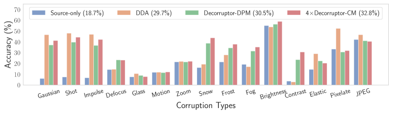
Figure 4: Bar graph of comparisons for performances between DDA and our Decorruptors on ImageNet-C using ResNet50.

LPIPS	IN-C($\uparrow$)	IN($\downarrow$)
DDA	0.421	0.608
Decorruptor-DPM	0.575	0.573

Table 5: LPIPS scores with clean and corrupted images.

	Avg. Acc (%)
TENT	43.02
+ Decorruptor-DPM	45.52
DeYO	48.61
+ Decorruptor-DPM	49.50

Table 6: Orthogonality with model updates.

Decorruptor	ResNet-50	Swin-T
DPM (0.42s)	30.5	37.8
CM (1step) (0.05s)	26.8	34.5
4$\times$CM (1step) (0.08s)	32.6	38.7
CM (4step) (0.10s)	27.5	35.6
4$\times$CM (4step) (0.14s)	32.8	39.7

Table 7: Variants of Decorruptor-CM.

5.3.3 Analysis on Decorruptor-CM

Table 7 reports the experimental results for various choices of Decorruptor-CM. When editing the input image only once for prediction, it is fast but the performance decreases by about 2-3% compared to Decorruptor-DPM. However, obtaining four edited images for each input and using their average prediction in Eq. (10) leads to higher accuracy than DPM, regardless of the architecture. Notably, even for the same corrupted image, Decorruptor allows diverse edits towards different clean images. The increasing performance gap between 1 step and 4 steps as the model size grows suggests that the quality of images is inferred to be better with 4 steps.

5.4 Video Test-Time Adaptation

Decorruptor demonstrates significantly improved runtime compared to DDA. This indicates that Decorruptor can be practically applied not only in the image domain but also in the video domain. Therefore, we evaluated Decorruptor on a corrupted video dataset [32]. To align with the temporal property of videos, we applied Text2Video-Zero [26] to enable Decorruptor to generate temporally consistent frames. Text2Video-Zero utilizes cross-frame attention from the first frame across the entire sequence, enabling temporally coherent editing. As shown in Fig. 6, our Decorruptor-CM demonstrated superior performance in corruption editing compared to the DDA method. Moreover, for a 3-second input video, our Deccoruptor takes almost 10 seconds for corruption editing while DDA takes almost 20 minutes for corruption editing. Consequently, we demonstrate that our Decorruptor provides highly effective and efficient video corruption editing. More detailed quantitative results can be found in the Appendix.

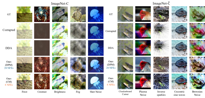
Figure 5: Illustration of the results of corruption editing for various corruptions at severity $5$. Consequently, we have verified that our Decorruptor-DPM and CM generally enable effective editing for test-time corruptions.

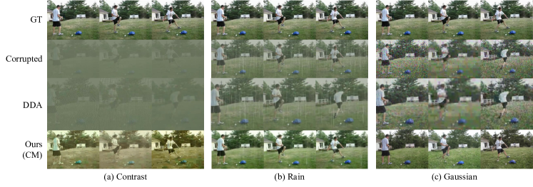
Figure 6: Results of corruption editing for corrupted videos in UCF101-C.

6 Conclusion and Future Work

The existing diffusion-based image-level updating TTA approach is robust to data order and batch size variations but is impractical for real-world usage due to its slow processing speed. In response, we propose Decorruptor-DPM, leveraging a latent diffusion model for efficient memory and time utilization. Through fine-tuning via our novel corruption modeling scheme, Decorruptor-DPM possesses the capability to edit corrupted images. Additionally, we introduce Decorruptor-CM, employing consistency distillation to accelerate input updates further. Decorruptor surpasses the baseline diffusion-based approach in speed by 100 times while delivering superior performance. Furthermore, Decorruptor achieves a threefold increase in speed and superior performance compared to the data augmentation-based model updating baseline. However, Decorruptor does not completely address the issue observed in DDA, where it exhibits lower performance than the source-only model for certain corruptions. Addressing the challenge of consistently restoring any type of corruption to a clean image remains an ongoing task for image-level updating TTA approaches.

Appendix 0.A Additional Results

0.A.1 Detailed Results of Image Corruption Editing

Tables 8 and 9 present detailed performance results of Decorruptor on ImageNet-C [15] and ImageNet-$\bar{\mathrm{C}}$ [39], respectively, using ResNet-50 [14] as the architecture. As shown in Table 1, Decorruptor demonstrates significant performance improvement for Noise and Weather corruptions. However, for some of Digital corruptions, it exhibits slightly lower performance than source-only for some specific corruptions. DDA [13] also shares the limitation of not being able to properly edit some corruptions. Addressing this issue is crucial for the effectiveness of the input updating TTA [59] method. As illustrated in Table 2, Our Decorruptor shows consistent improvement for all corruptions in ImageNet-$\bar{\mathrm{C}}$. Commonly, ensembling more edited images always presents performance improvement for all corruptions in ImageNet-C and ImageNet-$\bar{\mathrm{C}}$. Further results of ensembling is provided in Section 0.A.5.

	Noise			Blur				Weather				Digital
ImageNet-C	Gauss.	Shot	Impul.	Defoc.	Glass	Motion	Zoom	Snow	Frost	Fog	Brit.	Contr.	Elastic	Pixel	JPEG	Avg.
ResNet-50 (Source-only)	6.1	7.5	6.7	14.4	7.6	11.8	21.4	16.2	21.4	19.1	55.1	3.6	14.5	33.3	42.1	18.7
$\bullet~{}$Decorruptor-DPM	37.1	39.7	36.7	23.3	8.9	11.5	21.4	38.7	34.4	31.5	56.3	23.5	22.4	30.6	41.0	30.5
$\bullet~{}$Decorruptor-CM	30.3	33.4	30.7	19.5	7.4	11.6	20.8	33.2	29.8	28.5	56.0	22.1	17.9	30.6	40.2	27.5
$\bullet~{}$4$\times$Decorruptor-CM	41.2	44.3	42.2	23.1	7.8	12.1	22.0	43.7	37.8	35.2	58.9	30.6	20.3	31.9	40.4	32.8
$\bullet~{}$8$\times$Decorruptor-CM	44.1	46.7	44.9	24.0	8.0	12.4	22.5	46.2	40.3	36.4	59.7	32.6	20.6	33.2	41.1	34.2

Table 8: Detailed results on ImageNet-C at severity level 5 regarding accuracy (%). The bold value signifies the top-performing result.

ImageNet-$\bar{\mathrm{C}}$	Blue.	Brown.	Caustic.	Checker.	Cocentric.	Inverse.	Perlin.	Plasma.	Single.	Sparkles	Avg.
ResNet-50 (Source-only)	23.7	41.3	37.7	32.7	4.2	9.3	46.3	9.9	4.6	48.1	25.8
$\bullet~{}$Decorruptor-DPM	38.6	53.5	45.3	45.4	31.5	26.6	54.8	34.0	30.6	58.1	41.8
$\bullet~{}$Decorruptor-CM	37.4	51.5	43.5	44.2	27.1	21.3	53.1	29.3	26.8	56.7	39.1
$\bullet~{}$4$\times$Decorruptor-CM	45.6	57.4	48.2	51.5	42.2	28.2	57.5	39.8	39.6	61.2	47.1
$\bullet~{}$8$\times$Decorruptor-CM	47.2	58.2	49.2	53.4	43.2	29.4	58.6	41.2	40.4	62.2	48.3

Table 9: Detailed results on ImageNet-$\bar{\mathrm{C}}$ at severity level 5 regarding accuracy (%). The bold value signifies the top-performing result.

0.A.2 Quantitative Video Corruption Editing Results

For our experiments, we referred to the performance chart of ViTTA (see Table. 2 in Lin et al. [32]). In this section, we describe the results obtained by applying Decorruptor-CM for video corruption editing. The UCF-101C [32] dataset includes 3,783 corrupted videos for each type of corruption, totaling 10 different corruptions. The entire process of video decorruption was conducted using eight A40 GPUs and took about three days. The network used in the experiments was TANet [34], and when combining the model update method with our approach, we did not use an ensemble but instead assessed the performance solely using the generated dataset. The results are described in Table. 10. As a result, when ensembling with the source, there was an average performance improvement of approximately 13% compared to source-only inference. These results suggest that our Decorruptor-CM can be effectively applied to video domains. Moreover, by applying our method with the TTA methodology, we confirmed an average performance improvement of about 3% compared to ViTTA, especially showing robust decorruption results against noise.

Update	Methods	Gauss	Pepper	Salt	Shot	Zoom	Impulse	Defocus	Motion	JPEG	Contrast	Rain	H265.abr	Avg
	Source-Only	17.92	23.66	7.85	72.48	76.04	17.16	37.51	54.51	83.40	62.68	81.44	81.58	51.35
Data	Ours-Only	42.43	54.24	33.01	85.83	75.83	56.25	37.82	58.33	85.77	74.83	85.85	81.97	64.34
	NORM [50]	45.23	42.43	27.91	86.25	84.43	46.31	54.32	64.19	89.19	75.26	90.43	83.27	65.77
	DUA [40]	36.61	33.97	22.39	80.25	77.13	36.72	44.89	55.67	85.12	30.58	82.66	78.14	55.34
	TENT [60]	58.34	53.34	35.77	89.61	87.68	59.08	64.92	75.59	90.99	82.53	92.12	85.09	72.92
Model	SHOT [31]	46.10	43.33	29.50	85.51	82.95	47.53	53.77	63.37	88.69	73.30	89.82	82.66	65.54
	T3A [21]	19.35	26.57	8.83	77.19	79.38	18.64	40.68	58.61	86.12	67.22	84.00	83.45	54.17
	ViTTA [32]	71.37	64.55	45.84	91.44	87.68	71.90	70.76	80.32	91.70	86.78	93.07	84.56	78.33
All	ViTTA + Ours	77.05	79.03	64.18	93.25	86.54	78.32	65.72	78.30	91.76	86.41	92.25	83.58	81.37

Table 10: Qualitative results for the UCF101-C dataset. Here, ‘Ours-Only’ refers to results obtained from inference using only input updates. We further provide the results of combining our methodology with the baseline TTA method.

0.A.3 Corruption Granularity

Our proposed Decorruptor-DPM and CM methodologies also exhibit superior decorruption capabilities across all levels of severity when compared with DDA [13]. Notably, as depicted in Fig. 7 (b), CM shows comparable results with DPM only with 4 NFEs while effectively preserving the object-centric regions of a given image. Note, background colors sometimes change due to the stochastic nature of the diffusion model.

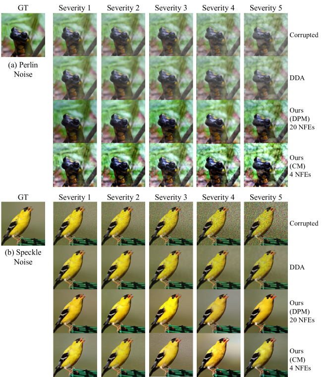
Figure 7: Visualization of corruption editing results based on the granularity of severity for various corruptions.

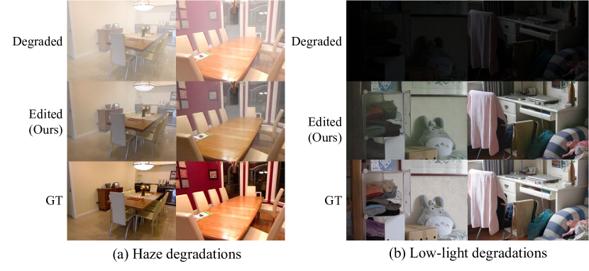
Figure 8: Further applications of our Decorruptor model in image restoration tasks.

0.A.4 Further Use-Cases

Furthermore, as depicted in Fig. 8, although such image degradations were not specifically learned in our U-Net fine-tuning stage, our Decorruptor-DPM shows the editing capabilities of corruptions like haze and low-light conditions. The datasets used for these examples are the Reside SOTS [29] and LOL [63] datasets, respectively.

0.A.5 Further Results of Ensemble

As shown in Table 7 of Section 5.3 in the main manuscript, the addition of ensemble in Decorruptor-CM led to performance improvement. However, without careful consideration, increasing the number of edited images required for ensemble results in drawbacks in terms of runtime and memory consumption. Therefore, the number of edited images also becomes a crucial hyperparameter. We illustrated the performance variations with the change in the number of images used for ensemble in ImageNet-C and ImageNet-$\bar{\mathrm{C}}$ in Figures 9 and 10, respectively. The results indicate a consistent performance increase regardless of the architecture as the number of edited images increases, and the performance tends to converge around 4 ensembles.

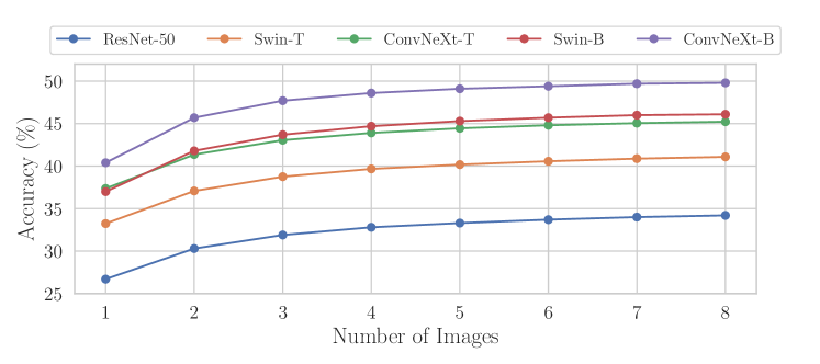
Figure 9: The accuracy (%) according to the number of edited images for ensembling in ImageNet-C

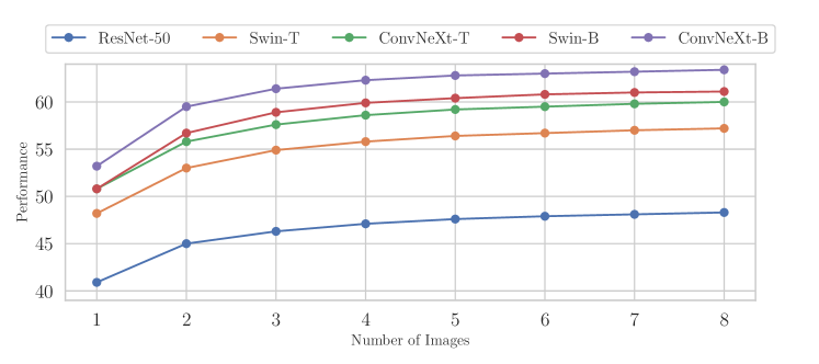
Figure 10: The accuracy (%) according to the number of edited images for ensembling in ImageNet-$\bar{\mathrm{C}}$

0.A.6 Diverse Corruption Scenarios, Image Sizes, and Domains

In this section, we presume a realistic situation when an image with various mixed corruptions is incoming at test time. We validate the editing performance for this scenario. For this experiment, we use Decorruptor-CM with 4 NFEs. As a result, as described in Fig. 11, we confirm that corruption editing is feasible with mixed corruption scenarios not only for (a) in-domain images but also for (b) out-of-domain images (e.g., panorama images). It is worth noting that we use mixed corruption severity as 5 for each corruption. Note that in each figure, the left side presents the corrupted images, while the right side displays the edited counterparts.

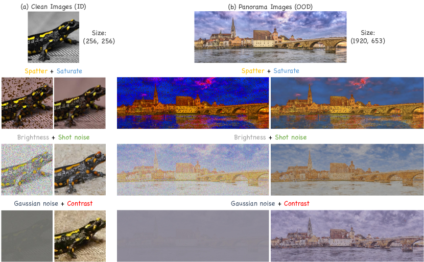
Figure 11: Visualization of experimental results on (a) in-domain, and (b) out-of-domain corruption editing performance. We confirmed that our proposed method robustly performs corruption editing even in scenarios where mixed corruption is presented at test time.

Appendix 0.B Ablation Studies

0.B.1 Image Guidance Scaling on Consistency Model

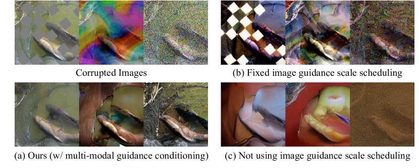
Figure 12: Ablation studies on (a) using the image guidance scale as conditioning, (b) fixed image guidance scale as 1.3, and (c) not using image guidance scale conditioning while distillation.

We describe the advantages of using the image guidance scale learnable in CM. LCM [37] shows fast convergence and a significant performance boost in distillation by using learnable guidance scales on SD. To extend LCM of SD to IP2P pipeline, we design a new learnable image guidance scale conditioning and enable multi-modal (i.e., image and text) conditioning.

For each ablation experiment in Fig. 12, we trained Decorruptor-CM for 12K iterations, consuming 24 GPU hours on an A40 GPU, respectively. As a result, as seen in (a), applying the proposed method by combining it with a text-guidance scale demonstrated the highest performance on corruption editing compared to others. For experiments, we use corruptions such as checkerboard, Brownian noise, and Gaussian noise. In the following, when the image guidance scale scheduling is not used for distillation, as shown in (b), we observe that weird images are generated. In the following in (c), when the guidance scale is fixed for distillation, editing is hardly performed, remaining close to the given image semantics. Here, the image guidance scale used is 1.3. Therefore, we confirm the importance of learnable image guidance scale conditioning on the distillation stage for effective corruption editing.

0.B.2 Using Other Fast Diffusion Schedulers

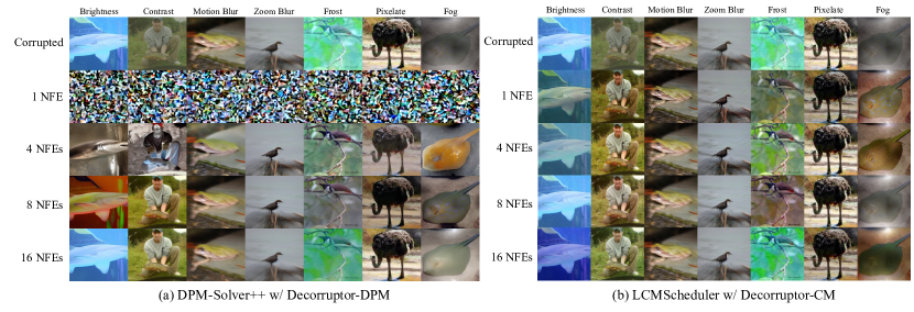
Figure 13: For several corruptions, (a) a combination of DPM and fast scheduler, (b) results of corruption editing according to the number of NFEs through CM. Note, we used the proposed multi-modal guidance scale conditioning method for the distillation of CM.

We conducted experiments based on the type of scheduler using the DPM-Solver++ sampler [36], traditionally utilized for fast sampling. The results, as shown in Fig. 13 (a), indicate that the sample quality of edited images dramatically decreases with smaller NFEs, and catastrophic failure occurs at 1 NFE. On the other hand, intriguingly, as shown in Fig, 13 (b), our Decorruptor-CM showed comparable corruption editing performance even at 1 NFE to that at 4 NFEs and confirmed better editing quality as the NFE increases. Therefore, this suggests that our proposed Decorruptor-CM enables fast, high-performance corruption editing. Each experiment was conducted with a fixed random seed.

Appendix 0.C Failure Cases

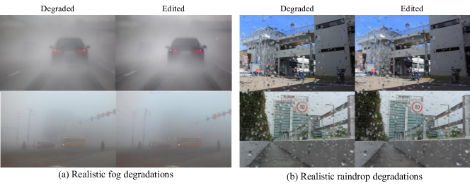
Figure 14: Failure cases of our model in scenarios involving realistic image degradations.

Although our method consistently outperforms other baselines, noticeable improvements were not observed in editing like blur, and pixelation corruptions. Furthermore, as illustrated in Fig. 14, when presented with more realistic degradations such as fog or raindrops, we have observed that our model exhibits limitations in corruption editing. Although containing paired datasets in the pre-training stage can resolve such realistic degradations, methods of how to edit such images at test-time without containing such realistic paired images (i.e., clean and corrupted) during training remain a challenging problem for TTA researchers.

References

- [1] Ai, Y., Huang, H., Zhou, X., Wang, J., He, R.: Multimodal prompt perceiver: Empower adaptiveness, generalizability and fidelity for all-in-one image restoration. arXiv preprint arXiv:2312.02918 (2023)
- [2] Baradad Jurjo, M., Wulff, J., Wang, T., Isola, P., Torralba, A.: Learning to see by looking at noise. Advances in Neural Information Processing Systems 34, 2556–2569 (2021)
- [3] Boudiaf, M., Mueller, R., Ben Ayed, I., Bertinetto, L.: Parameter-free online test-time adaptation. In: Proceedings of the IEEE/CVF Conference on Computer Vision and Pattern Recognition. pp. 8344–8353 (2022)
- [4] Brooks, T., Holynski, A., Efros, A.A.: Instructpix2pix: Learning to follow image editing instructions. In: Proceedings of the IEEE/CVF Conference on Computer Vision and Pattern Recognition. pp. 18392–18402 (2023)
- [5] Chen, X., He, K.: Exploring simple siamese representation learning. In: Proceedings of the IEEE/CVF conference on computer vision and pattern recognition. pp. 15750–15758 (2021)
- [6] Choi, J., Kim, S., Jeong, Y., Gwon, Y., Yoon, S.: Ilvr: Conditioning method for denoising diffusion probabilistic models. arXiv preprint arXiv:2108.02938 (2021)
- [7] Chung, H., Kim, J., Mccann, M.T., Klasky, M.L., Ye, J.C.: Diffusion posterior sampling for general noisy inverse problems. In: The Eleventh International Conference on Learning Representations (2023), https://openreview.net/forum?id=OnD9zGAGT0k
- [8] Chung, H., Ye, J.C., Milanfar, P., Delbracio, M.: Prompt-tuning latent diffusion models for inverse problems. arXiv preprint arXiv:2310.01110 (2023)
- [9] Cubuk, E.D., Zoph, B., Mane, D., Vasudevan, V., Le, Q.V.: Autoaugment: Learning augmentation strategies from data. In: Proceedings of the IEEE/CVF conference on computer vision and pattern recognition. pp. 113–123 (2019)
- [10] Deng, J., Dong, W., Socher, R., Li, L.J., Li, K., Fei-Fei, L.: Imagenet: A large-scale hierarchical image database. In: 2009 IEEE conference on computer vision and pattern recognition. pp. 248–255. Ieee (2009)
- [11] Dhariwal, P., Nichol, A.: Diffusion models beat gans on image synthesis. Advances in neural information processing systems 34, 8780–8794 (2021)
- [12] Ganin, Y., Lempitsky, V.: Unsupervised domain adaptation by backpropagation. In: International conference on machine learning. pp. 1180–1189. PMLR (2015)
- [13] Gao, J., Zhang, J., Liu, X., Darrell, T., Shelhamer, E., Wang, D.: Back to the source: Diffusion-driven test-time adaptation. arXiv preprint arXiv:2207.03442 (2022)
- [14] He, K., Zhang, X., Ren, S., Sun, J.: Deep residual learning for image recognition. In: Proceedings of the IEEE conference on computer vision and pattern recognition. pp. 770–778 (2016)
- [15] Hendrycks, D., Dietterich, T.: Benchmarking neural network robustness to common corruptions and perturbations. Proceedings of the International Conference on Learning Representations (2019)
- [16] Hendrycks, D., Zou, A., Mazeika, M., Tang, L., Li, B., Song, D., Steinhardt, J.: Pixmix: Dreamlike pictures comprehensively improve safety measures. In: Proceedings of the IEEE/CVF Conference on Computer Vision and Pattern Recognition. pp. 16783–16792 (2022)
- [17] Hertz, A., Mokady, R., Tenenbaum, J., Aberman, K., Pritch, Y., Cohen-Or, D.: Prompt-to-prompt image editing with cross attention control. arXiv preprint arXiv:2208.01626 (2022)
- [18] Ho, J., Jain, A., Abbeel, P.: Denoising diffusion probabilistic models. Advances in neural information processing systems 33, 6840–6851 (2020)
- [19] Ho, J., Salimans, T.: Classifier-free diffusion guidance. arXiv preprint arXiv:2207.12598 (2022)
- [20] Hwang, U., Lee, J., Shin, J., Yoon, S.: SF(DA)$^2$: Source-free domain adaptation through the lens of data augmentation. In: The Twelfth International Conference on Learning Representations (2024), https://openreview.net/forum?id=kUCgHbmO11
- [21] Iwasawa, Y., Matsuo, Y.: Test-time classifier adjustment module for model-agnostic domain generalization. Advances in Neural Information Processing Systems 34, 2427–2440 (2021)
- [22] Jiang, Y., Zhang, Z., Xue, T., Gu, J.: Autodir: Automatic all-in-one image restoration with latent diffusion. arXiv preprint arXiv:2310.10123 (2023)
- [23] Karras, T., Aittala, M., Aila, T., Laine, S.: Elucidating the design space of diffusion-based generative models. Advances in Neural Information Processing Systems 35, 26565–26577 (2022)
- [24] Kawar, B., Elad, M., Ermon, S., Song, J.: Denoising diffusion restoration models. Advances in Neural Information Processing Systems 35, 23593–23606 (2022)
- [25] Kawar, B., Elad, M., Ermon, S., Song, J.: Denoising diffusion restoration models. In: Advances in Neural Information Processing Systems (2022)
- [26] Khachatryan, L., Movsisyan, A., Tadevosyan, V., Henschel, R., Wang, Z., Navasardyan, S., Shi, H.: Text2video-zero: Text-to-image diffusion models are zero-shot video generators. arXiv preprint arXiv:2303.13439 (2023)
- [27] Lee, J., Jung, D., Lee, S., Park, J., Shin, J., Hwang, U., Yoon, S.: Entropy is not enough for test-time adaptation: From the perspective of disentangled factors. In: The Twelfth International Conference on Learning Representations (2024)
- [28] Lee, J., Jung, D., Yim, J., Yoon, S.: Confidence score for source-free unsupervised domain adaptation. In: International Conference on Machine Learning. pp. 12365–12377. PMLR (2022)
- [29] Li, B., Ren, W., Fu, D., Tao, D., Feng, D., Zeng, W., Wang, Z.: Reside: A benchmark for single image dehazing. arXiv preprint arXiv:1712.04143 1, 5 (2017)
- [30] Liang, J., Hu, D., Feng, J.: Do we really need to access the source data? source hypothesis transfer for unsupervised domain adaptation. In: International conference on machine learning. pp. 6028–6039. PMLR (2020)
- [31] Liang, J., Hu, D., Feng, J.: Do we really need to access the source data? source hypothesis transfer for unsupervised domain adaptation. In: International conference on machine learning. pp. 6028–6039. PMLR (2020)
- [32] Lin, W., Mirza, M.J., Kozinski, M., Possegger, H., Kuehne, H., Bischof, H.: Video test-time adaptation for action recognition. In: Proceedings of the IEEE/CVF Conference on Computer Vision and Pattern Recognition. pp. 22952–22961 (2023)
- [33] Liu, Z., Lin, Y., Cao, Y., Hu, H., Wei, Y., Zhang, Z., Lin, S., Guo, B.: Swin transformer: Hierarchical vision transformer using shifted windows. In: Proceedings of the IEEE/CVF international conference on computer vision. pp. 10012–10022 (2021)
- [34] Liu, Z., Wang, L., Wu, W., Qian, C., Lu, T.: Tam: Temporal adaptive module for video recognition. In: Proceedings of the IEEE/CVF international conference on computer vision. pp. 13708–13718 (2021)
- [35] Liu, Z., Mao, H., Wu, C.Y., Feichtenhofer, C., Darrell, T., Xie, S.: A convnet for the 2020s. In: Proceedings of the IEEE/CVF conference on computer vision and pattern recognition. pp. 11976–11986 (2022)
- [36] Lu, C., Zhou, Y., Bao, F., Chen, J., Li, C., Zhu, J.: Dpm-solver++: Fast solver for guided sampling of diffusion probabilistic models. arXiv preprint arXiv:2211.01095 (2022)
- [37] Luo, S., Tan, Y., Huang, L., Li, J., Zhao, H.: Latent consistency models: Synthesizing high-resolution images with few-step inference. arXiv preprint arXiv:2310.04378 (2023)
- [38] Meng, C., Rombach, R., Gao, R., Kingma, D., Ermon, S., Ho, J., Salimans, T.: On distillation of guided diffusion models. In: Proceedings of the IEEE/CVF Conference on Computer Vision and Pattern Recognition. pp. 14297–14306 (2023)
- [39] Mintun, E., Kirillov, A., Xie, S.: On interaction between augmentations and corruptions in natural corruption robustness. Advances in Neural Information Processing Systems 34, 3571–3583 (2021)
- [40] Mirza, M.J., Micorek, J., Possegger, H., Bischof, H.: The norm must go on: Dynamic unsupervised domain adaptation by normalization. In: Proceedings of the IEEE/CVF conference on computer vision and pattern recognition. pp. 14765–14775 (2022)
- [41] Nakashima, K., Kataoka, H., Matsumoto, A., Iwata, K., Inoue, N., Satoh, Y.: Can vision transformers learn without natural images? In: Proceedings of the AAAI Conference on Artificial Intelligence. vol. 36, pp. 1990–1998 (2022)
- [42] Nie, W., Guo, B., Huang, Y., Xiao, C., Vahdat, A., Anandkumar, A.: Diffusion models for adversarial purification. arXiv preprint arXiv:2205.07460 (2022)
- [43] Niu, S., Wu, J., Zhang, Y., Chen, Y., Zheng, S., Zhao, P., Tan, M.: Efficient test-time model adaptation without forgetting. In: International conference on machine learning. pp. 16888–16905. PMLR (2022)
- [44] Niu, S., Wu, J., Zhang, Y., Wen, Z., Chen, Y., Zhao, P., Tan, M.: Towards stable test-time adaptation in dynamic wild world. arXiv preprint arXiv:2302.12400 (2023)
- [45] Park, C., Lee, J., Yoo, J., Hur, M., Yoon, S.: Joint contrastive learning for unsupervised domain adaptation. arXiv preprint arXiv:2006.10297 (2020)
- [46] Parmar, G., Kumar Singh, K., Zhang, R., Li, Y., Lu, J., Zhu, J.Y.: Zero-shot image-to-image translation. In: ACM SIGGRAPH 2023 Conference Proceedings. pp. 1–11 (2023)
- [47] Rombach, R., Blattmann, A., Lorenz, D., Esser, P., Ommer, B.: High-resolution image synthesis with latent diffusion models. In: Proceedings of the IEEE/CVF conference on computer vision and pattern recognition. pp. 10684–10695 (2022)
- [48] Ronneberger, O., Fischer, P., Brox, T.: U-net: Convolutional networks for biomedical image segmentation. In: Medical Image Computing and Computer-Assisted Intervention–MICCAI 2015: 18th International Conference, Munich, Germany, October 5-9, 2015, Proceedings, Part III 18. pp. 234–241. Springer (2015)
- [49] Saito, K., Watanabe, K., Ushiku, Y., Harada, T.: Maximum classifier discrepancy for unsupervised domain adaptation. In: Proceedings of the IEEE conference on computer vision and pattern recognition. pp. 3723–3732 (2018)
- [50] Schneider, S., Rusak, E., Eck, L., Bringmann, O., Brendel, W., Bethge, M.: Improving robustness against common corruptions by covariate shift adaptation. Advances in neural information processing systems 33, 11539–11551 (2020)
- [51] Schuhmann, C., Beaumont, R., Vencu, R., Gordon, C., Wightman, R., Cherti, M., Coombes, T., Katta, A., Mullis, C., Wortsman, M., et al.: Laion-5b: An open large-scale dataset for training next generation image-text models. Advances in Neural Information Processing Systems 35, 25278–25294 (2022)
- [52] Sohl-Dickstein, J., Weiss, E., Maheswaranathan, N., Ganguli, S.: Deep unsupervised learning using nonequilibrium thermodynamics. In: International conference on machine learning. pp. 2256–2265. PMLR (2015)
- [53] Sohn, K., Berthelot, D., Carlini, N., Zhang, Z., Zhang, H., Raffel, C.A., Cubuk, E.D., Kurakin, A., Li, C.L.: Fixmatch: Simplifying semi-supervised learning with consistency and confidence. Advances in neural information processing systems 33, 596–608 (2020)
- [54] Song, J., Meng, C., Ermon, S.: Denoising diffusion implicit models. arXiv preprint arXiv:2010.02502 (2020)
- [55] Song, Y., Dhariwal, P., Chen, M., Sutskever, I.: Consistency models (2023)
- [56] Song, Y., Ermon, S.: Generative modeling by estimating gradients of the data distribution. Advances in neural information processing systems 32 (2019)
- [57] Song, Y., Sohl-Dickstein, J., Kingma, D.P., Kumar, A., Ermon, S., Poole, B.: Score-based generative modeling through stochastic differential equations. arXiv preprint arXiv:2011.13456 (2020)
- [58] Soomro, K., Zamir, A.R., Shah, M.: Ucf101: A dataset of 101 human actions classes from videos in the wild. arXiv preprint arXiv:1212.0402 (2012)
- [59] Wang, D., Shelhamer, E., Liu, S., Olshausen, B., Darrell, T.: Tent: Fully test-time adaptation by entropy minimization. arXiv preprint arXiv:2006.10726 (2020)
- [60] Wang, D., Shelhamer, E., Liu, S., Olshausen, B., Darrell, T.: Tent: Fully test-time adaptation by entropy minimization. arXiv preprint arXiv:2006.10726 (2020)
- [61] Wang, Q., Fink, O., Van Gool, L., Dai, D.: Continual test-time domain adaptation. In: Proceedings of the IEEE/CVF Conference on Computer Vision and Pattern Recognition. pp. 7201–7211 (2022)
- [62] Wang, Y., Yu, J., Zhang, J.: Zero-shot image restoration using denoising diffusion null-space model. arXiv preprint arXiv:2212.00490 (2022)
- [63] Wei, C., Wang, W., Yang, W., Liu, J.: Deep retinex decomposition for low-light enhancement. arXiv preprint arXiv:1808.04560 (2018)
- [64] Yun, S., Han, D., Oh, S.J., Chun, S., Choe, J., Yoo, Y.: Cutmix: Regularization strategy to train strong classifiers with localizable features. In: Proceedings of the IEEE/CVF international conference on computer vision. pp. 6023–6032 (2019)
- [65] Zhang, H., Cisse, M., Dauphin, Y.N., Lopez-Paz, D.: mixup: Beyond empirical risk minimization. arXiv preprint arXiv:1710.09412 (2017)
- [66] Zhang, L., Rao, A., Agrawala, M.: Adding conditional control to text-to-image diffusion models. In: Proceedings of the IEEE/CVF International Conference on Computer Vision. pp. 3836–3847 (2023)
- [67] Zhang, M., Levine, S., Finn, C.: Memo: Test time robustness via adaptation and augmentation. Advances in Neural Information Processing Systems 35, 38629–38642 (2022)
- [68] Zhang, R., Isola, P., Efros, A.A., Shechtman, E., Wang, O.: The unreasonable effectiveness of deep features as a perceptual metric. In: Proceedings of the IEEE conference on computer vision and pattern recognition. pp. 586–595 (2018)
- [69] Zhao, H., Liu, Y., Alahi, A., Lin, T.: On pitfalls of test-time adaptation. In: International Conference on Machine Learning (ICML) (2023)