Impulsive Lorenz semiflows: Physical measures,
statistical stability and entropy stability

Abstract.

We study semiflows generated via impulsive perturbations of Lorenz flows. We prove that such semiflows admit a finite number of physical measures. Moreover, if the impulsive perturbation is small enough, we show that the physical measures of the semiflows are close, in the weak* topology, to the unique physical measure of the Lorenz flow. A similar conclusion holds for the entropies associated with the physical measures.

1. Introduction

Lorenz [31] studied numerically the three-dimensional vector field defined by

$$\left\{\begin{array}[]{l}\dot{x_{1}}=\sigma(x_{2}-x_{1}),\\ \dot{x_{2}}=rx_{1}-x_{2}-x_{1}x_{3},\\ \dot{x_{3}}=x_{1}x_{2}-bx_{3},\end{array}\right.$$ (1.1)

when $\sigma=10$, $r=28$ and $b=8/3$, as a simplified model for atmospheric convection. By numerical calculations, Lorenz observed that the associated flow has a compact trapping region with a chaotic attractor. Later, a rigorous mathematical framework of similar flows, called geometric Lorenz flows, was introduced in [3, 28]. In [37], Tucker provided a computer-assisted proof that the classical Lorenz attractor is indeed a geometric Lorenz attractor. In particular, it is a singular-hyperbolic attractor [32], namely a nontrivial robustly transitive attracting invariant set containing a singularity (equilibrium point). Moreover, it admits a unique physical measure; see for example [11]. Recently, many authors studied the stability of such physical measure and other statistical properties under small smooth perturbations of Lorenz flows [9, 12, 13]. It is know that invariant stable foliations of Lorenz flows persist under small smooth perturbations; see for instance [18]. In particular, the associated Poincaré map inherits an invariant $C^{1+\alpha}$, $\alpha>0$, stable foliation [10] and the Poincaré map can be represented by a two dimensional skew product, where the base map is a one-dimensional piecewise uniformly expanding and the fibre maps are uniformly contracting. Such properties were exploited in [9, 12, 13].

Impulsive perturbations are very common in physical models. They capture phenomena characterised by sudden changes in the states of the system (e.g. when billiard balls collide, there is an impulse exchanged between them, resulting in abrupt changes in their velocities and directions). In this work, we are interested in studying impulsive perturbations of Lorenz flows, where the resulting perturbations generate discontinuous impulsive semiflows (see Subsection 1.2 for a precise definition of an impulsive semiflow). Our motivation is twofold, on the one hand is to investigate stability of statistical properties for Lorenz flows under discontinuous perturbations, and on the other hand to investigate smooth ergodic theoretic properties in the context of impulsive dynamical systems; in particular, existence and stability of physical measures. The latter systems have been mainly studied from a qualitative point of view: existence and uniqueness of solutions, sufficient conditions to ensure a complete characterization and some asymptotic stability of the limit sets [14, 15, 16, 17, 22, 23, 30], with few exceptions on basic ergodic theoretic results [2, 7, 8].

Our work demonstrates how introducing a small impulsive perturbation to Lorenz flows can pose non-obvious problems, requiring techniques different from those traditionally employed in classical scenarios. At the technical level, the main difficultly in our study is that the perturbed semiflow is not continuous. Hence, in general, it is not expected that it admits a smooth invariant foliation. Consequently, to prove existence of physical measures for the semiflow through a corresponding Poincaré map, one cannot use the standard technique of quotienting along stable leaves, since the Poincaré map is not necessarily a skew product. We believe that the current work will stimulate further research on statistical properties for impulsive semiflows.

In the rest of this introduction, we recall the definition of a physical measure and the notion of an impulsive dynamical system. Statements of our main results (Theorem A and Theorem B) on existence and stability of physical measures and the corresponding entropies for impulsive Lorenz semiflows are found in Subsection 1.3.

1.1. Physical measures and $u$-Gibbs measures

Let $M$ be a finite dimensional compact Riemannian manifold (possibly with boundary) and $m$ be the Lebesgue (volume) measure on the Borel sets of $M$. We say that $X:\mathbb{R}^{+}_{0}\times M\to M$ is a semiflow if, for all $x\in M$ and $s,t\in\mathbb{R}^{+}_{0}$, we have

1. $X_{0}(x)=x$,

2. $X_{t+s}(x)=X_{t}(X_{s}(x))$.

The trajectory of $x\in M$ is the curve defined by $X_{t}(x)$, for $t\geq 0$. The semiflow is called a flow when we have $\mathbb{R}$ playing the role of $\mathbb{R}^{+}_{0}$, which means that we can consider the past of the trajectories.

Given a semiflow $X$ on $M$, we define the basin $\mathcal{B}_{\nu}$ of a probability measure $\nu$ on the Borel sets of $M$ as the set of points $x\in M$ such that, for any continuous $\varphi:M\to\mathbb{R}$, we have

$$\lim_{T\rightarrow\infty}\frac{1}{T}\int_{0}^{T}\varphi(X_{t}(x))dt=\int\varphi\,d\nu.$$ (1.2)

We say that $\nu$ is a physical measure for $X$ if $m(\mathcal{B}_{\nu})>0$. Since measures defined on the Borel sets of a compact metric space are determined by their integrals on continuous functions, it follows that distinct physical measures must have disjoint basins.

Physical measures for semiflows are frequently obtained considering discrete-time dynamical systems associated with these flows, e.g. via Poincaré return maps. In the discrete-time case of a dynamical system defined by a map $f:M\to M$, we define the basin $\mathcal{B}_{\mu}$ of a probability measure $\mu$ on the Borel sets of $M$ as the set of points $x\in M$ such that, for any continuous $\varphi:M\to\mathbb{R}$, we have

$$\lim_{n\rightarrow\infty}\frac{1}{n}\sum_{j=0}^{n-1}\varphi(f^{j}(x))dt=\int\varphi\,d\mu.$$ (1.3)

We say that $\mu$ is a physical measure for $f$ if $m(\mathcal{B}_{\mu})>0$. Note that a physical measure is necessarily $f$-invariant.

A probability measure $\mu$ on the Borel sets of $M$ is called a $u$-Gibbs measure (also known as an SRB measure) for a map ${f:M\to M}$ if i) $\mu$ is $f$-invariant, ii) $f$ has positive Lyapunov exponents $\mu$ almost everywhere, and iii) the conditional measures of $\mu$ on local unstable manifolds are absolutely continuous with respect to the Lebesgue measures on these manifolds. A result due to Pesin [33] establishes that if $f$ is a $C^{1+\alpha}$ diffeomorphism whose Lyapunov exponents are all nonzero with respect to an ergodic invariant probability measure $\mu$, then the stable holonomy is absolutely continuous. Using Birkhoff Ergodic Theorem, it can be proved that the basin of an ergodic probability measure $\mu$ in a compact Riemannian manifold $M$ contains $\mu$ almost every point in $M$; see e.g. [5, Proposition 2.12]. Since time averages with respect to continuous functions are constant on stable manifolds, it follows that every ergodic $u$-Gibbs probability measure for a $C^{1+\alpha}$ diffeomorphism with non-zero Lyapunov exponents $\mu$ almost everywhere is a physical measure. These conclusions, relatively well known for diffeomorphisms of class $C^{1+\alpha}$, are also valid for the class of piecewise $C^{1+\alpha}$ diffeomorphims considered in [35, 36] which we will address in this work; see also [29, Part I & Part II].

The existence of $u$-Gibbs measure for piecewise piecewise hyperbolic diffeomorphisms has been deduced in several situations under additional assumptions:

• bounded derivative [24, 19, 38, 39];

• conservative setting (billiards) [21, 20, 39];

• invariant stable foliation [11, 26];

• stable cone field transverse to the singularity set [25];

None of these assumptions are a priori verified for the Poincaré maps we consider. The most suitable work for our setting is that of Pesin [34] and Satayev [35, 36] on piecewise hyperbolic diffeomorphisms.

1.2. Impulsive semiflows

Consider a semiflow or a flow $X$ on $M$ and $\Sigma\subset M$ a region such that

$$\inf\left\{t>0:X_{t}(x)\in\Sigma\right\}>0,\quad\forall x\in M.$$

Given a map $\varphi:\Sigma\to M$ and $x\in M$, we define the impulsive trajectory ${\gamma_{x}:[0,T(x))\to M}$, for some $T(x)\in\mathbb{R}^{+}\cup\{\infty\}$, and the impulsive times $0=\tau_{0}(x)<\tau_{1}(x)<\tau_{2}(x)<\cdots$ (a finite or infinite number of times) using the following inductive procedure:

1. Set

   $$\tau_{1}(x)=\begin{dcases}\inf\left\{t>0:X_{t}(x)\in\Sigma\right\},&\text{if }X_{t}(x)\in\Sigma\text{ for some }t>0;\\ +\infty,&\text{otherwise;}\end{dcases}$$

   and for $0\leq t<\tau_{1}(x)$

   $$\gamma_{x}(t)=X_{t}(x).$$

   

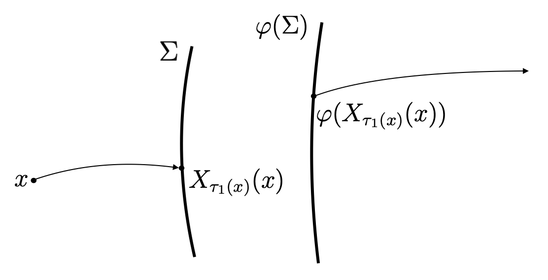
   Figure 1. Impulsive trajectory

2. Assume that $\tau_{n}(x)$ and $\gamma_{x}(t)$ have been defined for $0\leq t<\tau_{n}(x)$ and $n\geq 1$.
   If $\tau_{n}(x)=\infty$, then set $T(x)=\infty$ and stop the process.
   If $\tau_{n}(x)<\infty$, set

   $$\quad\quad\gamma_{x}(\tau_{n}(x))=\varphi(X_{\tau_{n}(x)-\tau_{n-1}(x)}(\gamma_{x}({\tau_{n-1}(x)}))),$$

   $$\tau_{n+1}(x)=\tau_{n}(x)+\tau_{1}(\gamma_{x}(\tau_{n}(x)))$$

   and for $\tau_{n}(x)<t<\tau_{n+1}(x)$

   $$\gamma_{x}(t)=X_{t-\tau_{n}(x)}(\gamma_{x}(\tau_{n}(x))).$$

   This completes the inductive procedure.

In case $\tau_{n}(x)<\infty$ for all $n\geq 1$, set

$$T(x)=\sup_{n\geq 1}\,\{\tau_{n}(x)\}.$$

In general we can have $T(x)=+\infty$ or $T(x)<+\infty$. However, assuming that $\varphi(\Sigma)\cap\Sigma=\emptyset$, it follows that $T(x)=+\infty$ for all $x\in M$; see [6, Remark 1.1]. We say that $(M,X,\Sigma,\varphi)$ is an impulsive dynamical system if

$$\tau_{1}(x)>0\quad\text{and}\quad T(x)=+\infty,\quad\text{for all $x\in M$}.$$

We call $\Sigma$ the impulsive region and $\varphi$ the impulsive map of the impulsive dynamical system. The impulsive semiflow $Y:\mathbb{R}^{+}_{0}\times M\to M$ of the impulsive dynamical system $(M,X,\Sigma,\varphi)$ is given by

$$Y(t,x)=\gamma_{x}(t),\quad\forall(x,t)\in\mathbb{R}^{+}_{0}\times M,$$

where $\gamma_{x}(t)$ is the impulsive trajectory of $x$ determined by $(M,X,\Sigma,\varphi)$. It follows from [14, Proposition 2.1] that $Y$ is indeed a semiflow, though not necessarily continuous nor a flow, even if $X$ is a flow. In fact, through the points of $\varphi(\Sigma)$ more than one trajectory can pass, which means that we cannot consider the past of these trajectories. A different type of impulsive perturbations was considered in [27].

1.3. Lorenz flows

Our main results will be obtained not only for the flow $X$ associated with the vector field in (1.1), but more generally for the broader class of geometric Lorenz flows introduced in [3, 28]. We will refer to all these flows as Lorenz flows. Many features of the flow $X$ in the trapping region $M$ have been proven over the last decades by studying the Poincaré return map to the plane $x_{3}=r-1$; see [3, 4]. As noted in [35, Section 2.2] and [36, Section 2] this return map fits in a certain set of conditions (L1)-(L4) that we describe in Subsection 2.2. In particular, using an appropriate coordinate system, the Poincaré return map is given by a transformation $F:\Sigma\to\Sigma$, where

$$\Sigma=\{(x_{1},x_{2},x_{3})\in\mathbb{R}^{3}:|x_{1}|\leq 1,\,|x_{2}|\leq 1,x_{3}=r-1\},$$

and has a discontinuity line $\Gamma\subset\Sigma$ given by $x_{1}=0$, dividing $\Sigma$ into the two subdomains such that $F$ is smooth in both subdomains. Strictly speaking, the transformation is not defined on the set $\Gamma$, but this is completely irrelevant for our purposes. It is well known that the return time $R:\Sigma\to\mathbb{R}^{+}$ at a point $x=(x_{0},x_{1},x_{3})\in\Sigma$ satisfies

$$R(x)\approx|\log|x_{0}||.$$ (1.4)

The return map $F$ has been exhaustively studied by several authors from various perspectives. In particular, it is well known that it admits a stable invariant foliation by nearly vertical lines, which makes it possible to obtain some of its properties studying the one-dimensional transformation in the quotient space by the stable leaves. This strategy was particularly successful in obtaining a $u$-Gibbs measure $\mu$ for $F$, which incidentally proves to be the unique physical measure for $F$, with its basin covering Lebesgue almost all of $\Sigma$. In the case of geometric Lorenz flows, the Poincaré return map $F$ and the return time $R$ enjoy these same properties by construction.

In this work we consider impulsive semiflows associated with Lorenz flows, having an impulsive map $\varphi:\Sigma\to M$ close to the inclusion map, with the impulsive region $\Sigma$ being the domain of a Poincaré return map as above. Allowing the impulsive map $\varphi$ to send points above $\Sigma$, it is relatively easy to think of examples for which the impulsive flow becomes essentially trivial. Indeed, consider a small $t_{0}>0$ and the impulsive map $\varphi:\Sigma\to M$ defined for each $x\in\Sigma$ by $\varphi(x)=X_{-t_{0}}(x).$ Since the trajectories under a Lorenz flow of Lebesgue almost all points in $M$ hit the region $\Sigma$, it follows that the trajectories of Lebesgue almost all points in $M$ enter a region where the flow is made up of periodic trajectories. We therefore consider the impulsive maps having images in a flow box below $\Sigma$, defined for some small $t_{0}>0$ as

$$B^{+}(\Sigma)=\{X_{t}(z):0<t\leq t_{0},\;z\in\Sigma\}.$$

Let the inclusion map of $\Sigma$ in $M$ be denoted by $\operatorname{inc}_{\Sigma}$, and the space of $C^{1}$ embeddings of $\Sigma$ in $M$ be denoted by $\operatorname{Emb}^{1}(\Sigma,M)$. Our first main result is the following theorem:

Theorem A.

Let $X$ be a Lorenz flow and $(M,X,\Sigma,\varphi)$ be an impulsive dynamical system such that $\varphi(\Sigma)\subset B^{+}(\Sigma).$ If $\varphi$ is a $C^{2}$ map sufficiently close to $\operatorname{inc}_{\Sigma}$ in $\operatorname{Emb}^{1}(\Sigma,M)$, then the semiflow associated with $(M,X,\Sigma,\varphi)$ has a finite number of physical measures whose basins cover Lebesgue almost all of $M$.

An interesting open problem is to investigate if the impulsive semiflow has a unique physical measure. Note that the uniqueness of the physical measure for Lorenz flows results from the uniqueness of the measure for the quotient transformation (because of transitivity), an instrument that we cannot use in our case. Uniqueness for the impulsive Lorenz semiflow will naturally follow from the uniqueness of the physical measures given by Corollary 3.4 for the Poincaré return map, something that is not guaranteed by the results in [35, 36].

A question that is of particular interest is whether the Lorenz flow is stable under small impulsive perturbations. We say that the Lorenz flow $X$ is statistically stable by impulsive perturbations on $\Sigma$ if, for any sequence $(\varphi_{n})_{n}$ converging to $\operatorname{inc}_{\Sigma}$ in the $C^{0}$ topology and any sequence $(\nu_{n})_{n}$, where $\nu_{n}$ is a physical measure for the impulsive flow of $(M,X,\Sigma,\varphi_{n})$, we have $\nu_{n}\to\nu$ in the weak* topology, as $n\to\infty$, where $\nu$ is the physical measure for $X$. We say that $X$ is entropy stable by impulsive perturbations on $\Sigma$ if $h_{\nu_{n}}(Y_{n})\to h_{\nu}(X)$, as $n\to\infty$, where each $Y_{n}$ is the impulsive semiflow of $(M,X,\Sigma,\varphi_{n})$ and $h_{(\cdot)}(\cdot)$ denotes the respective metric entropy. Our second main result is the following theorem:

Theorem B.

Lorenz flows are statistically stable and entropy stable by impulsive perturbations on $\Sigma$.

2. Piecewise hyperbolic diffeomorphisms

This section is devoted to the presentation of some results in [35, 36] for piecewise hyperbolic diffeomorphisms that will play an important role in this work. Let $\Sigma$ be a compact finite dimensional Riemannian manifold, possibly with a boundary. Denote by $\rho$ the distance in $\Sigma$ and by $m$ the Lebesgue measure on $\Sigma$. We say that $f:\Sigma\rightarrow\Sigma$ is a piecewise diffeomorphism if there exists a finite number of pairwise disjoint open regions $D_{1},\dots,D_{q}$ such that $\Sigma=\mskip 1.5mu\overline{\mskip-1.5mu{\cup_{i=1}^{q}{{D}}_{i}}\mskip-1.5mu}\mskip 1.5mu$ and $f|_{\cup_{i}D_{i}}$ is an injective differentiable map. Set

$$D=\cup_{i=1}^{q}D_{i}\quad\text{and}\quad\Gamma=\Sigma\setminus D.$$

We shall refer to $\Gamma$ as the singularity set of $f$ and assume $m(\Gamma)=0$. The derivative of $f$ at a point $x\in D$ will be denoted by $d_{x}f:T_{x}\Sigma\to T_{f(x)}\Sigma$.

2.1. Physical and $u$-Gibbs measures

The results on the existence of $u$-Gibbs measures for piecewise differentiable diffeomorphisms are obtained in [35, 36] under some hyperbolicity assumptions that will be stated below. First of all, we assume the existence of an unstable confield $(\mathcal{K}_{x}^{u})_{x\in D}$ and a stable conefield $(\mathcal{K}_{x}^{s})_{x\in D}$; see [35, Section 1.3] for precise definitions. We say that a submanifold $V\subset D$ is a u-disk (resp. s-disk) of size $r>0$ if it is a ball of radius $r$ in its intrinsic metric and the tangent space $T_{x}V$ is contained in $K_{x}^{u}$ (resp. $K_{x}^{s}$) for every $x\in V$. The Lebesgue measure on a $u$-disk $V$ will be denoted by $m_{V}$.

1. There are constants $A,\alpha>0$ such that, for any $x\in D$,

   $$\|d_{x}f\|\leq A\rho(x,\Gamma)^{-\alpha}\quad\text{and}\quad\|d^{2}_{x}f\|\leq A\rho(x,\Gamma)^{-\alpha}.$$

2. There are conefields $(\mathcal{K}_{x}^{u})_{x\in D}$ and $(\mathcal{K}_{x}^{s})_{x\in D}$ such that, for any $x\in D$,

   $$d_{x}f(\mathcal{K}_{x}^{u})\subset\mathcal{K}_{f(x)}^{u}\quad\text{and}\quad(d_{x}f)^{-1}(\mathcal{K}_{f(x)}^{s})\subset\mathcal{K}_{x}^{s}.$$

   Moreover, there exists $\lambda>1$ such that for any vectors $v\in\mathcal{K}_{x}^{u}$ and $w\in\mathcal{K}_{f(x)}^{s}$

   $$\|d_{x}f(v)\|\geq\lambda\|v\|\quad\text{and}\quad\|(d_{x}f)^{-1}(w)\|\geq\lambda\|w\|.$$

3. There are constants $B,\beta>0$ such that, for any $n\in\mathbb{N}$ and $\varepsilon>0$,

   $$m(f^{-n}(\Gamma_{\varepsilon}))<B\varepsilon^{\beta}.$$

4. There is $\varepsilon_{0}>0$ such that, for any $u$-disk $V$ there are $n_{0}=n_{0}(V)$ and $B_{0}=B_{0}(V)$ such that for any $\varepsilon\in(0,\varepsilon_{0})$,

   $$m_{V}(V\cap f^{-n}(\Gamma_{\varepsilon}))<\varepsilon^{\beta}m_{V}(V),\quad\forall n\geq n_{0},$$

   $$m_{V}(V\cap f^{-n}(\Gamma_{\varepsilon}))<B_{0}\varepsilon^{\beta}m_{V}(V),\quad\forall n\in\mathbb{N}.$$

5. The partition $D_{1},\dots,D_{q}$ is generating: for any $\varepsilon>0$, there is $n=n(\varepsilon)$ such that for any $j_{-n},\dots,j_{n}\in\{1,\dots,q\}$ the diameter of $\cap_{i=-n}^{n}f^{i}(D_{j_{i}})$ is smaller than $\varepsilon$.

6. There exist $\lambda>1$ and $r_{0}>0$ such that

   1. for any points $x,y$ in the same $s$-disk of size $r_{0}$ contained in $f(D_{j})$

      $$\rho(f^{-1}(x),f^{-1}(y))>\lambda\rho(x,y).$$

   2. for any points $x,y$ in the same $u$-disk of size $r_{0}$

      $$\rho(f(x),f(y))>\lambda\rho(x,y).$$

7. The constants $n_{0}(V)$ and $B_{0}(V)$ depend only on the size of $V$.

Conditions (H1)-(H5) are enough for ensuring the existence of $u$-Gibbs measures, the remaining (H6)-(H7) will be used to deduce the continuity of the $u$-Gibbs measures in the weak* topology under some additional assumptions to be presented in Subsection 2.3.

Theorem 2.1.

If $f$ satisfies (H1)-(H4), then there is a finite number of physical measures $\mu^{1},\dots,\mu^{s}$ for $f$ with $m(\Sigma\setminus(\mathcal{B}_{\mu^{1}}\cup\cdots\mathcal{B}_{\mu^{s}}))=0$ such that, for each $1\leq i\leq s$, we have

1. $\mu^{i}$ is an ergodic $u$-Gibbs measure;

2. the entropy formula holds for $\mu^{i}$;

3. there exists $A_{i}$ with $\mu^{i}(A_{i})=1$ such that Lebesgue almost every point in $\mathcal{B}_{\mu^{i}}$ belongs in the stable manifold of some point in $A_{i}$;

4. the densities of the conditionals of $\mu^{i}$ with respect to the Lebesgue measure on local unstable manifolds are bounded from above and below by uniform constants.

The conclusions of this theorem were essentially all obtained in [34, Theorem 2 and 3] with a countable number of measures. The above formulation with reduction to a finite number of measures follows from [35, Theorems 5.14 and 5.15], with the exception of the last item, which is not explicitly stated in [35], but still follows from the results therein. In fact, consider the set $D^{-}$ of points whose negative trajectories are defined and do not hit the singularity set $\Gamma$, i.e.

$$D^{-}=\bigcap_{n=1}^{\infty}f^{n}(D).$$

Set for $r>0$ and $\chi\in(0,1)$

$$M^{-}(r,\chi) =\left\{x\in D^{-}:\rho(f^{-n}(x),\Gamma)\geq r\chi^{n},\;\text{for all $n\geq 0$}\right\}.$$

For each $x\in M^{-}(r,\chi)$, there exists a local unstable manifold $V=V^{u}_{loc}(x,\delta(r))$ and, moreover, the conditional measure of each $\mu=\mu^{i}$ on $V$ is given as

$$\mu_{V}(E)=\int_{V\cap E}p(y)dm_{V}(y),$$

where $m_{V}$ is Lebesgue measure on $V$. In addition, for all $y\in V$,

$$p(y)=\frac{1}{\int_{V}q(y,z)dm_{V}}q(y,z),$$ (2.1)

and it follows from the Corollary after [35, Lemma 5.13] that there are constants $\gamma>\alpha$ and $C>0$ such that

$$|q(y,z)-1|<Cr^{\gamma-\alpha}.$$ (2.2)

This gives that last item of Theorem 2.1.

Remark 2.2.

The estimates in [35] give that the constants $C$ and $\gamma$ in (2.2) only depend on the constants involved in (H1)-(H4).

2.2. Lorenz maps

We present here a set of conditions given in [36, Section 2], defining a class of piecewise hyperbolic diffeomorphisms that satisfy conditions (H1)-(H7) and includes the two-dimensional Poincaré return map $F:\Sigma\to\Sigma$ associated with the Lorenz flow in an appropriate coordinate system.

1. The domain $\Sigma$ is the square $\{(x,y):|x|\leq 1,\,|y|\leq 1\}\subset\mathbb{R}^{2}$ and the curve $\Gamma\subset\Sigma$, given by $x=0$, divides $\Sigma$ into two subdomains

   $$D_{1}=\{(x,y)\in\Sigma:x>0\}\quad\text{and}\quad D_{2}=\{(x,y)\in\Sigma:x<0\}.$$

2. The map $f$ is smooth in both domains $D_{1}$ and $D_{2}$.

3. The map $f$ is given by $f(x,y)=(G(x,y),H(x,y))$, with

   $$\|H_{y}\|<1\quad\text{and}\quad\|G^{-1}_{x}\|<1,$$

   $$1-\|H_{y}\|\cdot\|G^{-1}_{x}\|>2\sqrt{\|G^{-1}_{x}\|\cdot\|H_{y}\|\cdot\|G^{-1}_{x}H_{x}\|},$$

   $$\|H_{y}\|\cdot\|G^{-1}_{x}H_{x}\|\cdot\|G_{y}\|<(1-\|H_{y}\|)(1-\|G^{-1}_{x}\|),$$

   where $G_{x},G_{y},H_{x}$ and $H_{y}$ denote the partial derivatives and $\|(x,y)\|=\sup\{|x|,|y|\}$.

4. Letting $G_{j},H_{j}$ denote respectively the restrictions of $G,H$ to $D_{j}$, for $j=1,2$, in a neighbourhood of $\Gamma$ the functions $G_{j}(x,y)$, $H_{j}(x,y)$ have the form

   $$G_{j}(x,y) =\tilde{G}_{j}(y|x|^{\beta},|x|^{\alpha}),$$

   $$H_{j}(x,y) =\tilde{H}_{j}(y|x|^{\beta},|x|^{\alpha}),$$

   with $\tilde{G}_{j},\tilde{H}_{j}$ smooth in a neighbourhood of $(0,0)$ and constants $\alpha\in(0,1)$ and $\beta>0$.

Theorem 2.3.

If $f$ satisfies (L1)-(L4), then $f$ satisfies (H1)-(H7).

See [36, Section 2 & Section 3] or the remark after [35, Theorem 2.1].

2.3. Statistical stability

Consider a sequence of piecewise hyperbolic diffeomorphisms $(f_{n})_{n}$ and $f$ such that (H1)-(H7) hold for all $f_{n}$ and $f$. For the conclusions about the continuity of $u$-Gibbs measures we need the following conditions.

1. The constants $A,\alpha,B,\beta,\lambda,\varepsilon_{0},B_{0}$ and the cones $\mathcal{K}^{u}_{x},\mathcal{K}^{s}_{x}$ appearing in (H1)-(H4) are the same for all $f$ and $f_{n}$.

2. The functions $f_{j}$ and $f_{n,j}$ have continuous extensions to the sets $D_{j}$ and $D_{n,j}$, respectively, for all $n$ and $j$.

3. The sets $D_{n,j}$ converge to the sets $D_{j}$, in the sense that for every $\varepsilon>0$ there is $n(\varepsilon)\in\mathbb{N}$ such that if $n>n(\varepsilon)$, then

   $$D_{j}\setminus\Gamma_{\varepsilon}\subset D_{n,j}\quad\text{and}\quad D_{n,j}\setminus\Gamma_{n,\varepsilon}\subset D_{j}.$$

4. The restriction of $f_{n}$ to $D_{n,j}$ is an equicontinuous family and it converges to the restriction of $f$ to $D_{j}$ in the $C^{0}$ topology.

5. On every $D_{j}\setminus\Gamma_{\varepsilon}$ the sequence $f_{n}$ converges to $f$ in the $C^{1}$ topology.

The next result is obtained in [35, Theorem 7.2].

Theorem 2.4.

Consider a sequence of maps $(f_{n})_{n}$ and $f$ such that conditions (H1)-(H7) and (S1)-(S5) hold for all $f_{n}$ and $f$. If $\mu_{n}$ is a $u$-Gibbs measure for $f_{n}$ and $\mu$ is a limit point of $\mu_{n}$ in the weak* topology, then $\mu$ is a $u$-Gibbs measure for $f$.

As a consequence of Theorem 2.1 and Theorem 2.4, we obtain the next result.

Corollary 2.5.

Consider a sequence of maps $(f_{n})_{n}$ and $f$ such that conditions (L1)-(L4) and (S1)-(S5) hold for all $f_{n}$ and $f$. If $\mu_{n}$ is a $u$-Gibbs measure for $f_{n}$ and $\mu$ is a limit point of $\mu_{n}$ in the weak* topology, then $\mu$ is a $u$-Gibbs measure for $f$.

3. Impulsive Lorenz semiflows

Consider $X$ the Lorenz flow defined in an open set $M\subset\mathbb{R}^{3}$ and $F:\Sigma\to\Sigma$ the Poincaré return map as described in Subsection 1.3. Let $\mu$ be the unique $u$-Gibbs measure for $F$. It is well known that the conditional measures of $\mu$ on local unstable manifolds have densities (with respect to Lebesgue measure) bounded from above and below by positive constants. Together with (1.4), this gives that the return time $R$ is integrable with respect to $\mu$. For a continuous function $\phi:M\to\mathbb{R}$, it is well known that the measure given by

$$\nu(\phi)=\frac{1}{\int_{\Sigma}Rd\mu}\int_{\Sigma^{\prime}}\int_{0}^{R(x)}\phi\circ X_{t}(x)dtd\mu(x)$$ (3.1)

is invariant under the Lorenz flow $X$; see Proposition 3.8 below for a proof in the case of impulsive perturbations of the Lorenz system (which contains the Lorenz system as the particular case $\varphi=\operatorname{inc}_{\Sigma}$). The entropy of the flow $X$ with respect to the measure $\nu$ is by definition the entropy of its time one map, i.e.

$$h_{\nu}(X)=h_{\nu}(X_{1})$$

By Abramov formula [1], we have

$$h_{\nu}(X)=\frac{h_{\mu}(F)}{\int_{\Sigma}Rd\mu}.$$ (3.2)

Consider from now on the impulsive dynamical system $(M,X,\Sigma,\varphi)$ as in Theorem A and the corresponding impulsive flow $Y$.

3.1. Poincaré return map

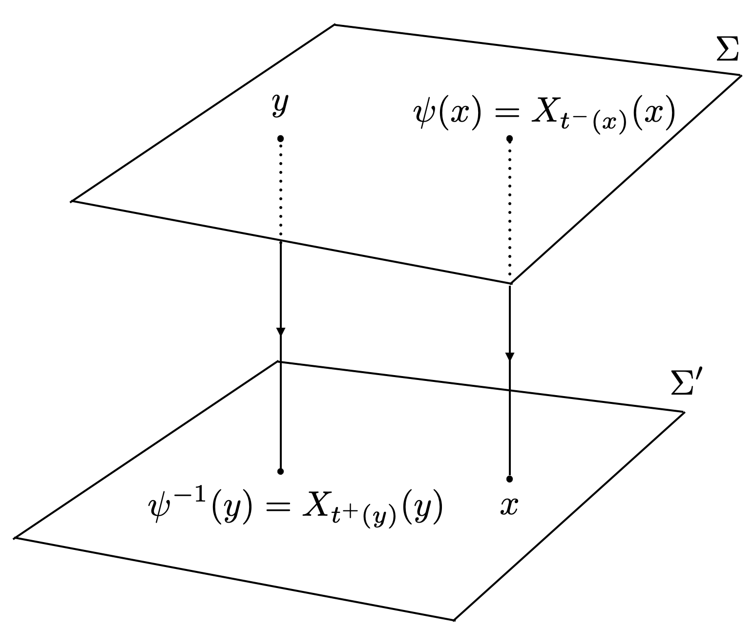
In this subsection we build a Poincaré return map for the impulsive semiflow $Y$. Assuming $\varphi$ is sufficiently close to $\operatorname{inc}_{\Sigma}\in\operatorname{Emb}^{1}(\Sigma,M)$, then $\Sigma^{\prime}=\varphi(\Sigma)$ is also a global cross section for $X$. We are going to define a Poincaré map for $Y$ on $\Sigma^{\prime}$. Since we assume $\Sigma^{\prime}\subset B^{+}(\Sigma)$, we have $\Sigma^{\prime}$ below $\Sigma$, with respect to the $z$ coordinate. For each $x\in\Sigma^{\prime}$, set

Figure 2. The maps $\psi$ and $\psi^{-1}$

$$t^{-}(x)=\max\{t<0:X_{t}(x)\in\Sigma\}$$ (3.3)

and for $y\in\Sigma$, set

$$t^{+}(y)=\min\{t>0:X_{t}(y)\in\Sigma^{\prime}\}.$$ (3.4)

Let $\psi:\Sigma^{\prime}\to\psi(\Sigma^{\prime})\subset\Sigma$ be the diffeomorphism given by

$$\psi(x)=X_{t^{-}(x)}(x),$$ (3.5)

with an inverse $\psi^{-1}:\psi(\Sigma^{\prime})\to\Sigma^{\prime}$ given by

$$\psi^{-1}(x)=X_{t^{+}(x)}(x).$$

The maps $t^{\pm}$, the section $\Sigma^{\prime}$ and the diffeomorphism $\psi$ depend on the impulsive system, but for simplicity we will not make this explicit in the notation at this stage, see Figure 2 for a pictorial illustration. We define the Poincaré map associated with the impulsive flow $F_{Y}:\Sigma^{\prime}\to\Sigma^{\prime}$ by

$$F_{Y}=\varphi\circ F\circ\psi.$$ (3.6)

Figure 3. The maps $F_{Y}$ and $\tilde{F}_{Y}$

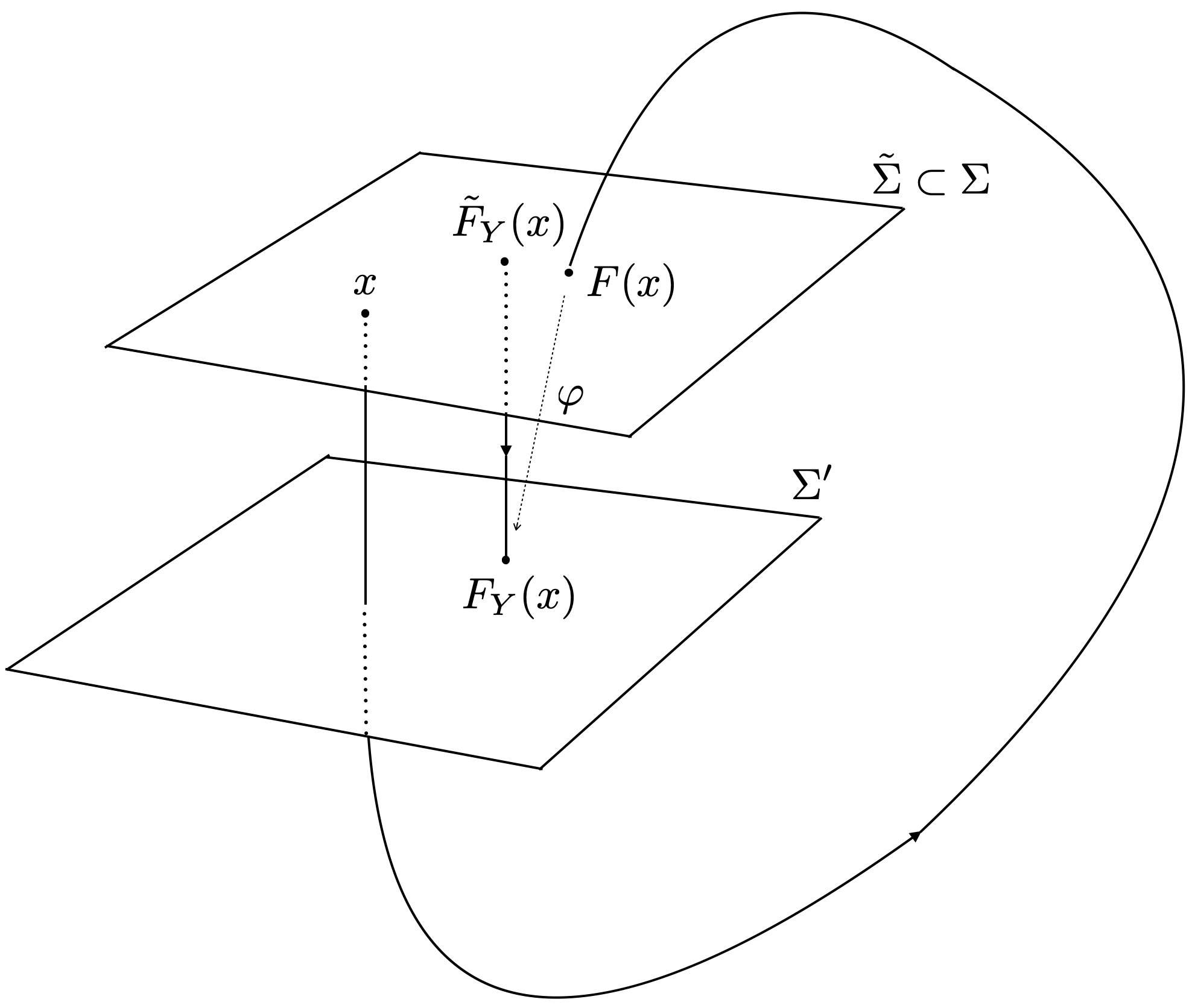
Observe that $F_{Y}$ is a piecewise $C^{1+\alpha}$ map with a singularity set $\Gamma_{Y}=\psi^{-1}(\Gamma)$. Actually, we are going to use a version of $F_{Y}$ translated to $\tilde{\Sigma}=\psi(\Sigma^{\prime})\subset\Sigma$, by considering $\tilde{F}_{Y}:\tilde{\Sigma}\to\tilde{\Sigma}$ defined by

$$\tilde{F}_{Y}=\psi\circ F_{Y}\circ\psi^{-1}.$$ (3.7)

Notice that $F_{Y}$ and $\tilde{F}_{Y}$ are conjugate dynamical systems via a smooth conjugacy, see Figure 3 for a pictorial illustration. It follows from (3.6) and (3.7) that

$$\tilde{F}_{Y}=\psi\circ\varphi\circ F.$$ (3.8)

Clearly, $\tilde{F}_{Y}$ has the same singularity set $\Gamma$ as $F$. Since $\varphi$ is a $C^{2}$ map close to $\operatorname{inc}_{\Sigma}$ in $\operatorname{Emb}^{1}(\Sigma,M)$, it follows that $\tilde{F}_{Y}$ is a small $C^{1+\alpha}$ perturbation of $F$. Notice however that $\tilde{F}_{Y}$ is not necessarily a Poincaré map for a Lorenz flow near $X$.

Remark 3.1.

Although $F$ has an invariant (stable) foliation, there is no guarantee that the same happens with $F_{Y}$ (and therefore also $\tilde{F}_{Y}$). The absence of such an invariant foliation and the consequent lack of existence of a quotient transformation, as in the Poincaré transformation of the Lorenz flow, make the study of the ergodic properties of $\tilde{F}_{Y}$ considerably more complicated than that of $F$.

Lemma 3.2.

$\tilde{F}_{Y}$ satisfies (L1)-(L4).

Proof.

It follows from  (3.8) that $\tilde{F}_{Y}$ has the same singularity set $\Gamma$ of $F$. Checking (L1)-(L2) is therefore just a matter of choosing the appropriate coordinate system. For (L3)-(L4), note that $\varphi$ (and hence $\psi$) can be taken arbitrarily close to the inclusion map and recall that $F$ satisfies (L3)-(L4); note also that the conditions in (L3) hold for small perturbations of $F$ and use (3.8) to obtain (L4). ∎

The previous lemma together with Theorem 2.1 yield the following conclusion.

Corollary 3.3.

If $\varphi$ is a $C^{2}$ map close to $\operatorname{inc}_{\Sigma}$ in $\operatorname{Emb}^{1}(\Sigma,M)$, then $\tilde{F}_{Y}$ has a finite number of physical measures $\tilde{\mu}^{1}_{Y},\dots,\tilde{\mu}^{s}_{Y}$ with $m(\tilde{\Sigma}\setminus(\mathcal{B}_{\tilde{\mu}_{Y}^{1}}\cup\cdots\mathcal{B}_{\tilde{\mu}_{Y}^{s}}))=0$ such that, for each $1\leq i\leq s$,

1. $\tilde{\mu}_{Y}^{i}$ is an ergodic $u$-Gibbs measure;

2. the entropy formula holds for $\tilde{\mu}_{Y}^{i}$;

3. there exists $A_{i}$ with $\tilde{\mu}^{i}_{Y}(A_{i})=1$ such that Lebesgue almost every point in $\mathcal{B}_{\tilde{\mu}^{i}_{Y}}$ belongs in the stable manifold of some point in $A_{i}$;

4. the densities of the conditionals of $\tilde{\mu}_{Y}^{i}$ with respect to the Lebesgue measure on local unstable manifolds are bounded from above and below by uniform constants.

Since (3.8) gives that $F_{Y}$ and $\tilde{F}_{Y}$ are conjugate dynamical systems via the smooth conjugacy $\psi$, we get the next consequence of Corollary 3.3.

Corollary 3.4.

If $\varphi$ is a $C^{2}$ map close to $\operatorname{inc}_{\Sigma}$ in $\operatorname{Emb}^{1}(\Sigma,M)$, then $F_{Y}$ has physical measures $\mu_{Y}^{1}=\psi^{-1}_{*}\mu_{Y}^{1},\dots,\mu_{Y}^{s}=\psi^{-1}_{*}\mu_{Y}^{s}$ with $m(\Sigma^{\prime}\setminus(\mathcal{B}_{\mu_{Y}^{1}}\cup\cdots\mathcal{B}_{\mu_{Y}^{s}}))=0$ such that, for each $1\leq i\leq s$,

1. $\mu_{Y}^{i}$ is an ergodic $u$-Gibbs measure;

2. the entropy formula holds for $\mu_{Y}^{i}$;

3. there exists $A_{i}$ with $\mu^{i}_{Y}(A_{i})=1$ such that Lebesgue almost every point in $\mathcal{B}_{\mu^{i}_{Y}}$ belongs in the stable manifold of some point in $A_{i}$;

4. the densities of the conditionals of $\mu_{Y}^{i}$ with respect to the Lebesgue measure on local unstable manifolds are bounded from above and below by uniform constants.

Remark 3.5.

Even though the Poincaré map $F$ for the Lorenz flow is transitive in the attractor (and thus it has a unique $u$-Gibbs measure) and $F_{Y}$ is a small perturbation of $F$, we cannot infer the transitivity of $F_{Y}$. This would be true if $F_{Y}$ were the Poincaré map of a Lorenz-like flow.

Note that the return time function $R_{Y}:\Sigma^{\prime}\to\mathbb{R}$ associated with the Poincaré map $F_{Y}$ for the impulsive semiflow $Y$ is related to the return time $R$ of the Lorenz flow $X$ by

$$R_{Y}=R\circ\psi+t^{-}.$$ (3.9)

In the following we simply use $\tilde{\mu}_{Y}$ to denote any of the measures given by Corollary 3.3.

Lemma 3.6.

$R\in L^{1}(\tilde{\mu}_{Y})$.

Proof.

Corollary 3.3 gives that the densities of the conditional measures of $\mu_{Y}$ with respect to Lebesgue measure on local unstable manifolds are bounded from above and below by uniform constants. Therefore, the integrability of $R$ with respect to $\tilde{\mu}_{Y}$ holds if it holds with respect to Lebesgue measure on $\Sigma$. The integrability with respect to Lebesgue measure is a consequence of the fact that $R$ satisfies (1.4). ∎

Corollary 3.7.

$R_{Y}\in L^{1}(\mu_{Y})$.

Proof.

It follows from (3.9) that

$$\int_{\Sigma^{\prime}_{Y}}R_{Y}d\mu_{Y}=\int_{\Sigma^{\prime}_{Y}}(R\circ\psi+t^{-})d\psi^{-1}_{*}\tilde{\mu}_{Y}=\int_{\tilde{\Sigma}_{Y}}(R+t^{-}\circ\psi^{-1})d\tilde{\mu}_{Y}.$$

Since $t^{-}\circ\psi^{-1}$ is a bounded function, the conclusion follows from Lemma 3.6. ∎

3.2. Physical measures

In this subsection we lift each physical measure of the Poincaré map $F_{Y}:\Sigma^{\prime}\to\Sigma^{\prime}$ to a physical measure of the impulsive semiflow $Y$. We perform the construction using standard ideas on suspension flows, taking into account the difficulties due the the lack of continuity of the impulsive semiflow.

First of all, we define a class of functions that will help us in defining the lifting. Consider $\mathcal{F}$ the class of bounded functions $\phi:M\to\mathbb{R}$ such that, for all $x\in\tilde{\Sigma}$, the function

$$\mathbb{R}\ni t\longmapsto\phi\circ Y_{t}(x)\in\mathbb{R}$$

has at most countably many discontinuity points. Clearly, $\mathcal{F}$ contains all the compositions $\phi\circ Y_{s}$, with $s\in\mathbb{R}^{+}_{0}$ and $\phi$ continuous, which obviously includes the continuous functions. Given an $F_{Y}$-invariant probability measure $\mu_{Y}$, set for $\phi\in\mathcal{F}$,

$$\nu_{Y}(\phi)=\frac{1}{\int_{\Sigma^{\prime}}R_{Y}d\mu_{Y}}\int_{\Sigma^{\prime}}\int_{0}^{R_{Y}(x)}\phi\circ Y_{t}(x)dtd\mu_{Y}(x),$$ (3.10)

where $dt$ stands for the integral with respect to the Lebesgue measure on $\mathbb{R}$, which is obviously well defined for all $\phi\in\mathcal{F}$.

Proposition 3.8.

$\nu_{Y}$ defines a probability measure on the Borel sets of $M$ which is invariant under the semiflow $Y$.

Proof.

It is straightforward to check that $\nu_{Y}$ is a linear positive functional on the set of continuous functions and that $\nu_{Y}(1)=1$. It follows from Riesz-Markov Theorem that $\nu_{Y}$ defines a probability measure on the Borel sets of $M$. The proof of the invariance of $\nu_{Y}$ follows essentially as in the case of a continuous flow, we include it here for completeness. We need to check that

$$\int\phi\circ Y_{s}d\nu_{Y}=\int\phi\circ d\nu_{Y}$$

for all continuous $\phi$. First of all, notice that the integral on the left hand side is well defined, since $\phi\circ Y_{s}\in\mathcal{F}$. Furthermore, setting $C=\left(\int_{\Sigma^{\prime}}R_{Y}d\mu_{Y}\right)^{-1}$, we may write

$$\int\phi\circ Y_{s}d\nu_{Y} =C\int_{\Sigma^{\prime}}\int_{0}^{R_{Y}(x)}\phi\circ Y_{s}\circ Y_{t}(x)dtd\mu_{Y}(x)$$

$$=C\int_{\Sigma^{\prime}}\int_{0}^{R_{Y}(x)}\phi\circ Y_{s+t}(x)dtd\mu_{Y}(x)$$

$$=C\int_{\Sigma^{\prime}}\int_{s}^{R_{Y}(x)+s}\phi\circ Y_{t}(x)dtd\mu_{Y}(x)$$

$$=C\int_{\Sigma^{\prime}}\left(\int_{0}^{R_{Y}(x)}\!\!\!\phi\circ Y_{t}(x)dt-\int_{0}^{s}\phi\circ Y_{t}(x)dt+\int_{R_{Y}(x)}^{R_{Y}(x)+s}\!\!\!\phi\circ Y_{t}(x)dt\right)d\mu_{Y}(x).$$

We are left to show that

$$\int_{\Sigma^{\prime}}\int_{0}^{s}\phi\circ Y_{t}(x)dtd\mu_{Y}(x)=\int_{\Sigma^{\prime}}\int_{R_{Y}(x)}^{R_{Y}(x)+s}\phi\circ Y_{t}(x)dtd\mu_{Y}(x).$$ (3.11)

Indeed, using the $F_{Y}$-invariance of $\mu_{Y}$ we get

$$\int_{\Sigma^{\prime}}\int_{0}^{s}\phi\circ Y_{t}(x)dtd\mu_{Y}(x) =\int_{0}^{s}\int_{\Sigma^{\prime}}\phi\circ Y_{t}(x)d\mu_{Y}(x)dt$$

$$=\int_{0}^{s}\int_{\Sigma^{\prime}}\phi\circ Y_{t}\circ F_{Y}(x)d\mu_{Y}(x)dt$$

$$=\int_{\Sigma^{\prime}}\int_{0}^{s}\phi\circ Y_{t}\circ F_{Y}(x)dtd\mu_{Y}(x)$$

$$=\int_{\Sigma^{\prime}}\int_{0}^{s}\phi\circ Y_{t}\circ Y_{R_{Y}(x)}(x)dtd\mu_{Y}(x)$$

$$=\int_{\Sigma^{\prime}}\int_{R_{Y}(x)}^{R_{Y}(x)+s}\phi\circ Y_{t}(x)dtd\mu_{Y}(x).$$

This gives (3.11), which concludes the proof. ∎

Let now $\mu_{Y}^{1},\dots,\mu_{Y}^{s}$ be the physical measures for the Poincaré return map $F_{Y}$ given by Corollary 3.4. Consider the probability measures $\nu_{Y}^{1},\dots,\nu_{Y}^{s}$ defined on the Borel sets of $M$, where each $\nu_{Y}^{i}$ is related to $\mu_{Y}^{i}$ through the formula in (3.10). With the next proposition we conclude the proof of Theorem A.

Proposition 3.9.

$\nu_{Y}^{1},\dots,\nu_{Y}^{s}$ are physical measures for $Y$ whose basins cover Lebesgue almost all of $M$.

Proof.

It is well known that with the exception of trajectories contained in the stable manifold of the singularity point 0, all other trajectories of points in the trapping region $M$ hit the Poincaré section $\Sigma$. This implies that the trajectories of Lebesgue almost all points in $M$ must intersect $\Sigma$. Taking into account the definition of the Poincaré map $F_{Y}$ for the impulsive semiflow $Y$, we easily get that the trajectories of Lebesgue almost all points in $M$ pass through $\Sigma^{\prime}$. Since the basin of a measure is invariant under the dynamics, it is enough to show that Lebesgue almost all points in $\Sigma^{\prime}$ belong in the basin of one of the measures $\nu_{Y}^{i}$, for some $i=1,\dots,s$.

By Corollary 3.4 we know that Lebesgue almost all points in $\Sigma^{\prime}$ belong in the basin of one of the ergodic measures $\mu_{Y}^{i}$, for some $i=1,\dots,s$. Moreover, there exists a set $A_{i}$ with $\tilde{\mu}^{i}_{Y}(A_{i})=1$ such that Lebesgue almost every point in $\mathcal{B}_{\tilde{\mu}^{i}_{Y}}$ belongs in the stable manifold of some point in $A_{i}$. Given a continuous function $\varphi:M\to\mathbb{R}$, consider $\varphi:\Sigma^{\prime}\to\mathbb{R}$ given for $x\in\Sigma^{\prime}$ by

$$\hat{\varphi}(x)=\int_{0}^{R_{Y}(x)}\varphi(Y_{t}(x))dt.$$

By Corollary 3.7 and Birkhoff’s Ergodic Theorem we may assume that for $\mu_{Y}^{i}$ almost every $x\in A_{i}$ we have

$$\lim_{n\rightarrow\infty}\frac{1}{n}\sum_{j=0}^{n-1}R_{Y}(F_{Y}^{j}(x))dt=\int_{\Sigma^{\prime}}R_{Y}\,d\mu_{Y}^{i}$$ (3.12)

and

$$\lim_{n\rightarrow\infty}\frac{1}{n}\sum_{j=0}^{n-1}\hat{\varphi}(F_{Y}^{j}(x))dt=\int_{\Sigma^{\prime}}\hat{\varphi}\,d\mu_{Y}^{i}.$$ (3.13)

Without loss of generality, we can also assume that

$$R_{Y}(F_{Y}^{n}(x))<\infty,\quad\text{for all $x\in A_{i}$ and $n\geq 0$.}$$ (3.14)

Given $x\in A_{i}$, set $T_{0}(x)=0$ and

$$T_{n}(x)=R_{Y}(x)+R_{Y}(F_{Y}(x))+\cdots+R_{Y}(F^{n-1}(x)),\quad\text{for $n\geq 1$.}$$

Given $T>0$, consider $n=n(T)\in\mathbb{N}$ such that $T_{n-1}(x)<T\leq T_{n}(x)$. By (3.14), such an integer $n$ always exists. Moreover,

$$T\to\infty\implies n\to\infty.$$ (3.15)

We may write

$$\frac{1}{T}\int_{0}^{T}\varphi(Y_{t}(x))dt =\frac{1}{T}\sum_{j=0}^{n-1}\int_{T_{j}(x)}^{T_{j+1}(x)}\!\!\!\varphi(Y_{t}(x))dt-\frac{1}{T}\int_{T}^{T_{n}(x)}\!\!\!\varphi(Y_{t}(x))dt$$

$$=\frac{1}{T}\sum_{j=0}^{n-1}\int_{0}^{R_{Y}(F_{Y}^{j}(x))}\!\!\!\varphi(Y_{t}(F_{Y}^{j}(x)))dt-\frac{1}{T}\int_{0}^{T_{n}(x)-T}\!\!\!\varphi(Y_{t}(F^{n}(x)))dt.$$ (3.16)

Using the definition of $\hat{\varphi}$, we get

$$\frac{1}{T}\sum_{j=0}^{n-1}\int_{0}^{R_{Y}(F_{Y}^{j}(x))}\varphi(Y_{t}(F_{Y}^{j}(x)))dt=\frac{1}{T}\sum_{j=0}^{n-1}\hat{\varphi}(F_{Y}^{j}(x))=\frac{n}{T}\cdot\frac{1}{n}\sum_{j=0}^{n-1}\hat{\varphi}(F_{Y}^{j}(x)).$$ (3.17)

Now observe that

$$\frac{T_{n-1}(x)}{n}<\frac{T}{n}\leq\frac{T_{n}(x)}{n},$$

which together with (3.12) and (3.15) yields

$$\lim_{T\to\infty}\frac{T}{n}=\frac{1}{\int_{\Sigma^{\prime}}R_{Y}\,d\mu_{Y}^{i}}.$$ (3.18)

Since the measure $\nu_{Y}^{i}$ is related to $\mu_{Y}^{i}$ through the formula in (3.10), it follows from (3.13) and (3.18) that

$$\lim_{T\to\infty}\frac{n}{T}\cdot\frac{1}{n}\sum_{j=0}^{n-1}\hat{\varphi}(F_{Y}^{j}(x)) =\frac{1}{\int_{\Sigma^{\prime}}R_{Y}\,d\mu_{Y}^{i}}\int_{\Sigma^{\prime}}\hat{\varphi}\,d\mu_{Y}^{i}$$

$$=\frac{1}{\int_{\Sigma^{\prime}}R_{Y}\,d\mu_{Y}^{i}}\int_{\Sigma^{\prime}}\int_{0}^{R_{Y}(x)}\varphi(Y_{t}(x))dtd\mu_{Y}^{i}$$

$$=\int_{M}\varphi d\nu_{Y}^{i}.$$

Recalling (3.16) and (3.17), we are left to show that

$$\lim_{T\to\infty}\frac{1}{T}\int_{0}^{T_{n}(x)-T}\!\!\!\varphi(Y_{t}(F^{n}(x)))dt=0.$$ (3.19)

Since

$$\left|\frac{1}{T}\int_{0}^{T_{n}(x)-T}\!\!\!\varphi(Y_{t}(F^{n}(x)))\right|\leq\frac{T_{n}(x)-T}{T}\sup|\varphi|\leq\frac{T_{n}(x)-T_{n-1}(x)}{T}\sup|\varphi|$$

it is enough to prove that

$$\lim_{T\to\infty}\frac{T_{n}(x)-T_{n-1}(x)}{T}=0$$

Indeed, writing

$$\frac{T_{n}(x)-T_{n-1}(x)}{T}=\frac{T_{n}(x)-T_{n-1}(x)}{n}\cdot\frac{n}{T},$$

and recalling (3.18), the conclusion follows from (3.12). ∎

4. Impulsive stability of Lorenz flows

In this section we prove both the statistical stability and the entropy stability stated in Theorem B. Recall that $F$, $R$ and $\mu$ are respectively the Poincaré map, the return time function and the (unique) $u$-Gibbs measure for the Poincaré map $F$ associated with the Lorenz flow $X$. Recall also that $\nu$ is the physical measure for the Lorenz flow $X$ defined by the formula in (3.1).

Let $(\varphi_{n})_{n}$ be a sequence of impulses converging to $\operatorname{inc}_{\Sigma}$ in the $C^{1}$ topology and let $\nu_{n}$ be a physical measure for the semiflow $(Y^{n}_{t})_{t}$ of the impulsive dynamical system $(M,X,\Sigma,\varphi_{n})$. Let $t^{-}_{n}$, $t^{+}_{n}$, $\psi_{n}$ and $R_{n}$ be functions respectively as in (3.3), (3.4), (3.5) and (3.9) for each of these impulsive dynamical systems. Let also $\tilde{F}_{n}:\tilde{\Sigma}_{n}\to\tilde{\Sigma}_{n}$ be related to $F_{n}:\Sigma^{\prime}_{n}\to\Sigma^{\prime}_{n}$ as in (3.7), where $\Sigma_{n}^{\prime}=\varphi_{n}(\Sigma)$, $\tilde{\Sigma}_{n}=\psi_{n}(\Sigma_{n}^{\prime})$ and $F_{n}$ is the Poincaré defined as in (3.6) for the impulsive flow $Y_{n}$. By Corollary 3.4, we have $\mu_{n}=(\psi_{n}^{-1})_{*}\tilde{\mu}_{n}$, where $\mu_{n}$ is a $u$-Gibbs measure for $F_{n}$ and $\tilde{\mu}_{n}$ is a $u$-Gibbs measure for $\tilde{F}_{n}$. Let $\nu_{n}$ be one of the physical measures for the impulsive flow $Y_{n}$ related to $\mu_{n}$ by the formula (3.10); recall Proposition 3.9.

Lemma 4.1.

(S1)-(S5) hold for the sequence $(\tilde{F}_{n})_{n}$ and $F$.

Proof.

By Lemma 3.2 we have that (L1)-(L4) are satisfied for $F$ and therefore for all $F_{n}$ with uniform constants in (L3)-(L4), since (3.8) is valid and $\varphi_{n},\psi_{n}$ can be taken arbitrarily close to the inclusion maps. Since the constants $A,\alpha,B,\beta,\lambda,\varepsilon_{0},B_{0}$ and the cones $\mathcal{K}^{u}_{x},\mathcal{K}^{s}_{x}$ appearing in (H1)-(H4) depend only on the constants in (L3)-(L4), then (S1) follows. For the other conditions note first $\Gamma_{n}=\Gamma$ and $D_{n,j}=D_{j}$, for $j=1,2$. Then conditions (S2), (S3) and (S5) are trivially satisfied and (S4) follows from (3.8). ∎

4.1. Statistical stability

In this subsection we obtain the statistical stability part of Theorem B. Since $F$ has a unique $u$-Gibbs measure, it follows from Corollary 2.5, Lemma 3.2 and Lemma 4.1 that

$$\tilde{\mu}_{n}\stackrel{{\scriptstyle w*}}{{\longrightarrow}}\mu,\quad\text{as $n\to\infty$.}$$ (4.1)

Note that we may consider $\tilde{\mu}_{n}$ as a measure on the set $\Sigma$, since $\tilde{\Sigma}_{n}\subset\Sigma$. We are left to show that $\nu_{n}\to\nu$ in the weak^∗ topology, as $n\to\infty$. Since the measures $\nu$ and $\nu_{n}$ are given by (3.1) and (3.10) respectively, we just need to prove that

1. $\displaystyle\int_{\Sigma^{\prime}_{n}}R_{n}d\mu_{n}\to\int_{\Sigma}Rd\mu$, as $n\to\infty$,

and for all continuous $\phi:M\to\mathbb{R}$

1. $\displaystyle\int_{\Sigma_{n}^{\prime}}\int_{0}^{R_{n}(x)}\phi\circ Y^{n}_{t}(x)dtd\mu_{n}(x)\to\int_{\Sigma}\int_{0}^{R(x)}\phi\circ X_{t}(x)dtd\mu(x)$, as $n\to\infty$.

This will be obtained in the Lemma 4.3 and Lemma 4.4 below. In the next lemma we give an auxiliary result which will be used several times below.

Lemma 4.2.

Assume that the following conditions hold:

1. there exists a sequence $(h_{n})_{n}$ of continuous functions from $\Sigma$ to $\mathbb{R}$ converging $\mu$-almost everywhere to $h\in L^{1}(\mu)$, with $h\in L^{1}(\tilde{\mu}_{n})$, for all $n\geq 1$;

2. there exists $g\in L^{1}(\mu)$ such that $g\geq 0$ and $|h_{n}|\leq g$, for all $n\geq 1$.

Then

$$\lim_{n\to\infty}\int_{\Sigma}hd\tilde{\mu}_{n}=\int_{\Sigma}hd\mu.$$

Proof.

We may write for any $n,k\geq 1$

$$\int_{\Sigma}hd\tilde{\mu}_{n}=\int_{\Sigma}(h-h_{k})d\tilde{\mu}_{n}+\int_{\Sigma}h_{k}d\tilde{\mu}_{n}.$$

Since the densities of the conditionals of each $\tilde{\mu}_{n}$ with respect to Lebesgue measure on local unstable manifolds are bounded from above and below by positive constants independent of $n$ (recall Remark 2.2), we may assume that the conditionals of $\tilde{\mu}_{n}$ are those of Lebesgue measure in the first integral of the last sum. Since the conditionals of $\mu$ with respect to Lebesgue measure on local unstable manifolds are also bounded from above and below by positive constants, it follows that $h_{k}$ converges pointwise to $h$ for Lebesgue almost every point on local unstable manifolds. Therefore, $\int_{\Sigma}(h-h_{k})d\tilde{\mu}_{n}$ converges to zero, by dominated convergence theorem. Hence, taking first limit in $n$ and then limit in $k$ in the second term, the conclusion follows by the weak* convergence in (4.1) and the dominated convergence theorem. ∎

Lemma 4.3.

$\displaystyle\int_{\Sigma^{\prime}_{n}}R_{n}d\mu_{n}\to\int_{\Sigma}Rd\mu$, as $n\to\infty$.

Proof.

It follows from (3.9) that for all $n$

$$R_{n}=R\circ\psi_{n}+t^{-}_{n},$$

which together with Corollary 3.4 yields

$$\int_{\Sigma^{\prime}_{n}}R_{n}d\mu_{n}=\int_{\Sigma^{\prime}_{n}}(R\circ\psi_{n}+t^{-}_{n})d(\psi_{n}^{-1})_{*}\tilde{\mu}_{n}=\int_{\tilde{\Sigma}_{n}}(R+t^{-}_{n}\circ\psi_{n}^{-1})d\tilde{\mu}_{n}.$$

Since $t^{-}_{n}\circ\psi_{n}^{-1}$ is uniformly small when $\varphi_{n}$ converges to $\operatorname{inc}_{\Sigma}$ in the $C^{0}$ topology and the support of $\tilde{\mu}_{n}$ is a subset of $\Sigma$, we just need to prove that

$$\int_{\Sigma}Rd\tilde{\mu}_{n}\to\int_{\Sigma}Rd\mu,\quad\text{as $n\to\infty$.}$$ (4.2)

Set for each $k\geq 1$

$$\hat{R}_{k}=\min\{R,k\}.$$

We conclude the proof using Lemma 4.2 with $h_{k}=\hat{R}_{k}$ and $h=g=R$. The conditions (c₁) and (c₂) are clearly verified, by Lemma 3.6 and recalling that $R$ is integrable with respect to the measure $\mu$. ∎

Lemma 4.4.

For any continuous $\phi:M\to\mathbb{R}$, we have

$$\lim_{n\to\infty}\int_{\Sigma_{n}^{\prime}}\int_{0}^{R_{n}(x)}\phi\circ Y^{n}_{t}(x)dtd\mu_{n}(x)=\int_{\Sigma}\int_{0}^{R(x)}\phi\circ X_{t}(x)dtd\mu(x).$$

Proof.

We have

$$\int_{\Sigma_{n}^{\prime}}\int_{0}^{R_{n}(x)}\phi\circ Y^{n}_{t}(x)dtd\mu_{n}(x) =\int_{\Sigma_{n}^{\prime}}\int_{0}^{R\circ\psi_{n}(x)+t^{-}_{n}(x)}\phi\circ Y^{n}_{t}(x)dtd(\psi_{n}^{-1})_{*}\tilde{\mu}_{n}(x)$$

$$=\int_{\tilde{\Sigma}_{n}}\int_{0}^{R(x)+t^{-}_{n}\circ\psi_{n}^{-1}(x)}\phi\circ Y^{n}_{t}\circ\psi_{n}^{-1}(x)dtd\tilde{\mu}_{n}(x)$$

Since for any $x\in\tilde{\Sigma}_{n}$

$$\int_{0}^{R(x)+t^{-}_{n}\circ\psi_{n}^{-1}(x)}\!\!\!\!\phi\circ Y^{n}_{t}\circ\psi_{n}^{-1}(x)dt=\int_{0}^{R(x)}\!\!\!\!\phi\circ Y^{n}_{t}\circ\psi_{n}^{-1}(x)dt+\int_{0}^{t^{-}_{n}\circ\psi_{n}^{-1}(x)}\!\!\!\!\phi\circ Y^{n}_{t}\circ\psi_{n}^{-1}(x)dt$$

and $t^{-}_{n}\circ\psi_{n}^{-1}$ can be made uniformly small when $\varphi_{n}$ converges to $\operatorname{inc}_{\Sigma}$ in the $C^{0}$ topology, we just need to prove that

$$\int_{\Sigma}\int_{0}^{R(x)}\phi\circ Y^{n}_{t}\circ\psi_{n}^{-1}(x)dtd\tilde{\mu}_{n}(x)\to\int_{\Sigma}\int_{0}^{R(x)}\phi\circ X_{t}(x)dtd\mu(x),\quad\text{when $n\to\infty$}.$$

Note that we may assume that $\tilde{\mu}_{n}$ is a measure on $\Sigma$. We have

$$\int_{\Sigma}\int_{0}^{R(x)} \phi\circ Y^{n}_{t}\circ\psi_{n}^{-1}(x)dtd\tilde{\mu}_{n}(x)-\int_{\Sigma}\int_{0}^{R(x)}\phi\circ X_{t}(x)dtd\mu(x)$$

$$= \int_{\Sigma}\int_{0}^{R(x)}(\phi\circ Y^{n}_{t}\circ\psi_{n}^{-1}(x)-\phi\circ X_{t}(x))dtd\tilde{\mu}_{n}(x)$$ (4.3)

$$+\int_{\Sigma}\int_{0}^{R(x)}\phi\circ X_{t}(x)dtd\tilde{\mu}_{n}(x)-\int_{\Sigma}\int_{0}^{R(x)}\phi\circ X_{t}(x)dtd\mu(x).$$ (4.4)

First we prove that the difference in (4.4) converges to 0 when $n\to\infty$. Indeed, set

$$h(x)=\int_{0}^{R(x)}\phi\circ X_{t}(x)dt$$

and for $k\geq 1$,

$$\hat{R}_{k}(x)=\min\{R(x),k\}\quad\text{and}\quad h_{k}(x)=\int_{0}^{\hat{R}_{k}(x)}\phi\circ X_{t}(x)dt.$$

We have

$$|h_{k}(x)|=\left|\int_{0}^{\hat{R}_{k}(x)}\phi\circ X_{t}(x)dt\right|\leq\int_{0}^{\hat{R}_{k}(x)}\left|\phi\circ X_{t}(x)\right|dt\leq C\hat{R}_{k}(x)\leq CR(x).$$

We conclude the proof using Lemma 4.2 with $g=CR$. The conditions (c₁) and (c₂) are clearly verified, by Lemma 3.6 and recalling that $R$ is integrable with respect to $\mu$.

We are left to prove that the term in (4.3) converges to 0 when $n\to\infty$. For simplicity, consider

$$g(t,x)=\phi\circ X_{t}(x)\quad\text{and}\quad g_{n}(t,x)=\phi\circ Y^{n}_{t}\circ\psi_{n}^{-1}(x),\quad\forall n\geq 1.$$

It is enough to show that

$$\int_{\Sigma}\int_{0}^{R(x)}|g_{n}(t,x)-g(t,x)|dtd\tilde{\mu}_{n}(x)\to 0$$

when $n\to\infty$. Since $\hat{R}_{k}(x)\to R(x)$, when $k\to\infty$, for $\tilde{\mu}_{n}$-almost every $x$, by monotone convergence theorem

$$\int_{\Sigma}\int_{0}^{R(x)}|g_{n}(t,x)-g(t,x)|dtd\tilde{\mu}_{n}(x) =\int_{\Sigma}\lim_{k\to\infty}\int_{0}^{\hat{R}_{k}(x)}|g_{n}(t,x)-g(t,x)|dtd\tilde{\mu}_{n}(x)$$

$$=\lim_{k\to\infty}\int_{\Sigma}\int_{0}^{\hat{R}_{k}(x)}|g_{n}(t,x)-g(t,x)|dtd\tilde{\mu}_{n}(x).$$

Since this last expression defines an increasing sequence in $k$ of nonnegative numbers, we just need to show that each term in that sequence can be made arbitrarily small (for $n$ sufficiently large). So, fix an arbitrary $\varepsilon>0$. Given any $k\in\mathbb{N}$, there exists $n_{\varepsilon}\in\mathbb{N}$ (depending only on $k$) such that for all $x\in\Sigma$ and $0\leq t\leq\hat{R}_{k}(x)$ (recall that $\hat{R}_{k}(x)\leq k$), we have

$$n\geq n_{\varepsilon}\implies|g_{n}(t,x)-g(t,x)|<\varepsilon.$$

Therefore, for any $n\geq n_{\varepsilon}$ we have

$$\int_{\Sigma}\int_{0}^{\hat{R}_{k}(x)}|g_{n}(t,x)-g(t,x)|dtd\tilde{\mu}_{n}(x) \leq\varepsilon\int_{\Sigma}\hat{R}_{k}(x)d\tilde{\mu}_{n}(x)\leq\varepsilon\int_{\Sigma}R(x)d\tilde{\mu}_{n}(x).$$

Now, by (4.2), we may choose a uniform constant $C>0$ such that $\int_{\Sigma}R(x)d\tilde{\mu}_{n}(x)\leq C$, for all $n\in\mathbb{N}$. This finishes the proof. ∎

4.2. Entropy stability

In this subsection we obtain the entropy stability part of Theorem B. Similar to (3.2), we have by Abramov formula

$$h_{\nu_{n}}(Y_{n})=\frac{h_{\mu_{n}}(F_{n})}{\int_{\Sigma^{\prime}_{n}}R_{n}d\mu_{n}}.$$ (4.5)

By (3.2) and (4.5), it is enough to prove that

$$\frac{h_{\mu_{n}}(F_{n})}{\int_{\Sigma^{\prime}_{n}}R_{n}d\mu_{n}}\longrightarrow\frac{h_{\mu}(F)}{\int_{\Sigma}Rd\mu},\quad\text{as $n\to\infty$}.$$

Since $(F_{n},\mu_{n})$ and $(\tilde{F}_{n},\tilde{\mu}_{n})$ are isomorphic dynamical systems, by Lemma 4.3 we just need to prove that

$$h_{\tilde{\mu}_{n}}(\tilde{F}_{n})\to h_{\mu}(F),\quad\text{as $n\to\infty$}.$$ (4.6)

It follows from Theorem 2.1, Theorem 2.3 and Lemma 3.2 that the entropy formula holds for both dynamical systems $(\tilde{F}_{n},\tilde{\mu}_{n})$ and $(F,\mu)$. Therefore, the convergence in (4.6) can be rephrased as

$$\int_{\Sigma}\log|\tilde{J}^{u}_{n}|d\tilde{\mu}_{n}\to\int_{\Sigma}\log|J^{u}|d\mu,\quad\text{as $n\to\infty$},$$ (4.7)

where $J_{n}^{u}$ and $J^{u}$ stand for the unstable Jacobians of $\tilde{F}_{n}$ and $F$, respectively.

Lemma 4.5.

$\displaystyle\lim_{n\to\infty}\int_{\Sigma}\log|\tilde{J}^{u}_{n}|d\tilde{\mu}_{n}=\int_{\Sigma}\log|J^{u}|d\mu$.

Proof.

We have

$$\int_{\Sigma}\log|\tilde{J}^{u}_{n}|d\tilde{\mu}_{n}- \int_{\Sigma}\log|J^{u}|d\mu$$

$$=\int_{\Sigma}\left(\log|\tilde{J}^{u}_{n}|-\log|J^{u}|\right)d\tilde{\mu}_{n}+\int_{\Sigma}\log|J^{u}|d\tilde{\mu}_{n}-\int_{\Sigma}\log|J^{u}|d\mu.$$ (4.8)

We first prove that the integral of the difference above converges to zero when $n\to\infty$. By Hadamard’s inequality and (H1), we have for all $x$

$$|\tilde{J}^{u}_{n}(x)|\leq\|d_{x}F_{n}\|\leq A\rho(x,\Gamma)^{-\alpha};$$ (4.9)

recall that the constant $A$ may be chosen uniform, by Lemma 4.1. Since the densities of the conditionals of each $\tilde{\mu}_{n}$ with respect to Lebesgue measure on local unstable manifolds are bounded from above and below by positive constants independent of $n$ (recall Remark 2.2), we may assume that the conditionals of $\tilde{\mu}_{n}$ are those of Lebesgue measure. Moreover, it follows from (S5) that $\log|\tilde{J}^{u}_{n}|$ converges pointwise to $\log|\tilde{J}^{u}|$, Lebesgue almost everywhere. Since $\log\rho(x,\Gamma)^{-\alpha}$ is integrable with respect to Lebesgue measure, using (4.9) and dominated convergence theorem we conclude that the integral of the difference in (4.8) converges to zero when $n\to\infty$.

We are left to show that the difference of the integrals in (4.8) goes to zero when ${n\to\infty}$. Decomposing both integrals into integrals on $D_{1}$ and $D_{2}$, and noticing that $\log|J^{u}|$ is continuous on both $D_{1}$ and $D_{2}$, the conclusion follows by the weak* convergence of $\tilde{\mu}_{n}$ to $\mu$ given by (4.1). ∎

References

- [1] L. M. Abramov. On the entropy of a flow, Dokl. Akad. Nauk SSSR, 128:873–875, 1959.
- [2] S. M. Afonso, E. Bonotto, J. Siqueira. On the ergodic theory of impulsive semiflows, arXiv:2206.13001, 2022.
- [3] V. S. Afraĭmovič, V. V. Bykov, and L. P. Shilnikov. The origin and structure of the Lorenz attractor. Dokl. Akad. Nauk SSSR, 234(2):336–339, 1977.
- [4] V. S. Afraĭmovič, V. V. Bykov, and L. P. Shilnikov. On attracting structurally unstable limit sets of Lorenz attractor type. Trudy Moskov. Mat. Obshch., 44:150–212, 1982.
- [5] J. F. Alves. Nonuniformly hyperbolic attractors. Geometric and probabilistic aspects. Springer Monographs in Mathematics. Springer, Cham, 2020.
- [6] J. F. Alves and M. Carvalho. Invariant probability measures and non-wandering sets for impulsive semiflows. J. Stat. Phys., 157(6):1097–1113, 2014.
- [7] J. F. Alves, M. Carvalho, and J. Siqueira. Equilibrium states for impulsive semiflows J. Math. Anal. Appl. 451(2): 839–857, 2017.
- [8] J. F. Alves, M. Carvalho, and C.H. Vásquez. A variational principle for impulsive semiflows, J. Differential Equations 259(8):4229–4252, 2015.
- [9] J.F. Alves and M. Soufi. Statistical stability of geometric Lorenz attractors. Fund. Math. 224(3):219–231, 2014.
- [10] V. Araújo and I. Melbourne. Existence and smoothness of the stable foliation for sectional hyperbolic attractors. Bull. Lond. Math. Soc., 49(2):351–367, 2017.
- [11] V. Araújo, M.J. Pacifico, E. Pujals, and M. Viana. Singular-hyperbolic attractors are chaotic. Trans. Amer. Math. Soc., 361:2431–2485, 2009.
- [12] W. Bahsoun, I. Melbourne and M. Ruziboev. Variance continuity for Lorenz flows. Annales Henri Poincaré, 21:1873–1892, 2020.
- [13] W. Bahsoun and M. Ruziboev. On the statistical stability of Lorenz attractors with a stable foliation. Ergodic Theory Dynam. Systems, 39(12):3169–3184, 2019.
- [14] E. M. Bonotto. Flows of characteristic in impulsive semidynamical systems. J. Math. Anal. Appl., 332(1):81–96, 2007.
- [15] E. M. Bonotto and M. Federson. Topological conjugation and asymptotic stability in impulsive semidynamical systems. J. Math. Anal. Appl., 326(2):869–881, 2007.
- [16] E. M. Bonotto and M. Federson. Limit sets and the Poincaré-Bendixson theorem in impulsive semidynamical systems. J. Differential Equations, 244(9): 2334–2349, 2008.
- [17] E. M. Bonotto and G. M. Souto. On the Lyapunov stability theory for impulsive dynamical systems. Topol. Methods Nonlinear Anal., 53(1):127–150, 2019.
- [18] R. T. Bortolotti. Physical measures for certain partially hyperbolic attractors on 3-manifolds, Ergodic Theory Dynam. Systems, 39(1):74–104, 2019.
- [19] N. Chernov. Statistical properties of piecewise smooth hyperbolic systems in high dimensions. Discrete Contin. Dynam. Systems, 5(2):425–448, 1999.
- [20] N. Chernov and H.-K. Zhang. Billiards with polynomial mixing rates. Nonlinearity, 18(4):1527–1553, 2005.
- [21] N. Chernov and H.-K. Zhang. A family of chaotic billiards with variable mixing rates. Stoch. Dyn., 5(4):535–553, 2005.
- [22] K. Ciesielski. On semicontinuity in impulsive dynamical systems. Bull. Pol. Acad. Sci. Math., 52(1):71–80, 2004.
- [23] K. Ciesielski. On stability in impulsive dynamical systems. Bull. Pol. Acad. Sci. Math., 52(1):81–91, 2004.
- [24] M.F. Demers and C. Liverani. Stability of Statistical Properties in Two-dimensional Piecewise Hyperbolic Maps. Trans. Amer. Math. Soc. 360(9):4777–4814, 2008.
- [25] M.F. Demers and H.-K. Zhang. Spectral analysis of hyperbolic systems with singularities. Nonlinearity, 27(3):379–433, 2014.
- [26] S. Galatolo and R. Lucena. Spectral gap and quantitative statistical stability for systems with contracting fibers and Lorenz-like maps. Discrete Contin. Dyn. Syst., 40(3):1309–1360, 2020.
- [27] M. Gianfelice and S. Vaienti. Stochastic stability of the classical Lorenz flow under impulsive type forcing. J. Stat. Phys., 181(1):163–211, 2020.
- [28] J. Guckenheimer and R. F. Williams. Structural stability of Lorenz attractors. Inst. Hautes Études Sci. Publ. Math., (50):59–72, 1979.
- [29] A. Katok, J.-M. Strelcyn, F. Ledrappier, and F. Przytycki. Invariant manifolds, entropy and billiards; smooth maps with singularities, volume 1222 of Lecture Notes in Mathematics. Springer-Verlag, Berlin, 1986.
- [30] S. K. Kaul. Stability and asymptotic stability in impulsive semidynamical systems. J. Appl. Math. Stochastic Anal., 7(4):509–523, 1994.
- [31] E. N. Lorenz. Deterministic non-periodic flow. J. Atmos. Sci., 20:130–141, 1963.
- [32] C. A. Morales, M. J. Pacífico, E. R. Pujals. Robust transitive singular sets for 3-flows are partially hyperbolic attractors or repellers. Ann. of Math. (2), 160(2):375–432, 2004.
- [33] J. B. Pesin. Families of invariant manifolds that correspond to nonzero characteristic exponents. Izv. Akad. Nauk SSSR Ser. Mat., 40(6):1332–1379, 1440, 1976.
- [34] Y. B. Pesin. Dynamical systems with generalized hyperbolic attractors: hyperbolic, ergodic and topological properties. Ergodic Theory Dynam. Systems, 12(1):123–151, 1992.
- [35] E.A. Sataev. Invariant measures for hyperbolic mappings with singularities. Russian Math. Surveys, 47(1):191–251, 1992.
- [36] E. A. Sataev. Gibbs measures for one-dimensional attractors of hyperbolic mappings with singularities. Izv. Ross. Akad. Nauk Ser. Mat., 56(6):1328–1344, 1992.
- [37] W. Tucker. The Lorenz attractor exists. C. R. Acad. Sci. Paris Sér. I Math., 328(12):1197–1202, 1999.
- [38] L.-S. Young. Bowen-Ruelle measures for certain piecewise hyperbolic maps. Trans. Amer. Math. Soc., 287(1):41–48, 1985.
- [39] L.-S. Young. Statistical properties of dynamical systems with some hyperbolicity. Ann. of Math. (2), 147(3):585–650, 1998.