Role of Coulomb Interaction in Valley Photogalvanic Effect

Abstract

We develop a theory of Coulomb interaction-related contribution to the photogalvanic current of electrons in two-dimensional non-centrosymmetric Dirac materials possessing a nontrivial structure of valleys and exposed to an external electromagnetic field. The valley photogalvanic effect occurs here due to the trigonal warping of electrons and holes’ dispersions in a given valley of the monolayer. We study the low-frequency limit of the external field: the field frequency is smaller than the temperature $T$, and the electron-electron and electron-hole scattering times are much larger than the electron-impurity scattering time. In this regime, we employ the Boltzmann transport equations and show that electron-hole scattering dominates electron-electron scattering in intrinsic semiconductors. Coulomb interaction-related contribution to the valley photogalvanic current can reduce the value of the bare photogalvanic current as these two currents flow in the opposite directions.

I Introduction

The influence of the Coulomb scattering, namely, electron-electron (e-e) and electron-hole (e-h) interaction, on the transport properties of solids is an active research area. At low temperatures, when particle-phonon scattering is frozen, the particle-particle scattering mechanisms may determine the temperate behaviour of transport coefficients, in particular, the Drude conductivity [1]. In Galilean-invariant systems with the parabolic spectrum, particle collisions do not affect the conductivity since the velocity is proportional to the particle momentum, and thus, the conservation of total momentum under e-e and h-h collisions results in the conservation of velocity. Nevertheless, in strongly disordered samples, elastic scattering on impurities plays sufficient role: impurities break the Galilean invariance, and then, the influence of particle collisions not only can be finite, but also it results in strong Coulomb-induced corrections to conductivity [2]. In particular, weak localization corrections and corrections to magneto-oscillation transport phenomena [3], including the Shubnikov–de Haas effect, can emerge.

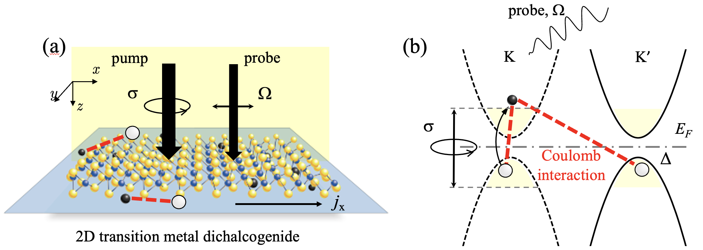
Figure 1: (a) System schematic: a 2D material exposed to a linearly polarized electromagnetic (EM) field with the frequency $\Omega$ and a circularly polarized light with the polarization $\sigma$. A circular-polarized EM field changes electron population at a given valley due to photoinduced interband transition, whereas a linearly polarized EM results in a valley photogalvanic effect (vPGE). (b) Reciprocal space of the 2D system, reflecting the multi-valley structure. Electrons scatter by holes in different valleys.

Interaction between charged particles can be repulsive or attractive, and it reveals different behavior in different temperature ranges. Indeed, in addition to the direct Coulomb repulsion between identical particles (e-e or h-h) and attraction of different particles (e-h in semiconductors), the other interaction channels may also strongly affect the conductivity of the material. In particular, strong particle-particle attraction in the Cooper channel leads to a renormalization of the Drude conductivity by superconducting fluctuations at sufficiently low temperatures (in the vicinity of the superconducting transition temperature). This constitutes the phenomenon referred to as the paraconductivity [4]. Furthermore, recent technological achievements open a way to creation of ultra-clean nanostructures, where the electron (and hole) mean free path, which is usually limited by the interaction with impurities, is comparable with or even exceeds the sample width [5, 6]. The system is in the hydrodynamic regime of electron transport [7, 8, 9]. In this regime, the particle momentum predominantly changes due to electron scattering off the sample boundaries. In some materials, the e-e and e-h interaction start to play a key role in the particle transport determining the viscosity of electron liquid.

This subject is especially timely for novel two-dimensional (2D) materials such as monolayers of graphene [10, 11] and transition-metal dichalcogenides (TMD) [12, 13, 14]. A key specifics of these materials is the two-valley structure of the dispersion of carriers of charge. Characteristic band structure results in the emergence of specific valley transport phenomena, such as the valley acoustoelectric effect and valley Hall effect [15, 16, 17, 18, 19, 20, 21]. Recently, both the diffusive and hydrodynamic regimes of valley Hall and anomalous Hall effects have been intensively studied theoretically [22, 23, 24]. One of the critical properties of electrons and holes in the valleys of TMD materials is the trigonal warping of valleys reflecting the trigonal symmetry of the crystal lattice. It results in the modification of the particle energy: $\epsilon_{\mathbf{p}}\approx p^{2}/2m+\eta w(p_{x}^{3}-3p_{x}p_{y}^{2})$, where $\mathbf{p}$ is the momentum of an electron or a hole, $m$ is the effective mass, $\eta=\pm 1$ is the valley index, and $w$ is the warping parameter. Thanks to that, in addition to the valley Hall effect, these materials reveal fascinating nonlinear transport phenomena such as the valley photogalvanic effect (vPGE) [25, 26, 27, 28]. From the mathematical point of view, the vPGE represents the second-order response of the stationary electric current density to the external alternating EM field with the frequency much smaller than the material bandgap.

There might exist various contributions to vPGE at small temperatures. For instance, attractive e-e interaction (the Cooper channel) can influence the magnitude of the vPGE [29]. Namely, the emergence of superconducting fluctuations strongly affect the vPGE in the vicinity of the superconducting transition temperature, obeying the law $(T-T_{c})^{-3}$ when $T\rightarrow T_{c}$ from above [29]. The goal of this paper is to examine the vPGE in TMDs due to particle-particle interaction in the Coulomb channel, when the temperature is high enough (or a particle density is low), thus the superconducting fluctuations do not play important role. In a previous work by some of the authors of this paper [26], bare vPGE in a non-degenerate electron gas was studied. Here, we will assume that the electron and hole gases are non-degenerate, satisfying the Boltzmann statistics, and apply the two-band model with the parabolic dispersion of electrons and holes with equal effective masses and accounting for the warping-related corrections to the parabolic dispersion. In an intrinsic MoS₂ at finite temperature, there can exist three channels of particle-particle interaction: e-e, h-h, and e-h ones. Our calculations show, that e-e and h-h contributions do not play role, despite small corrections to the warping and, consequently, to the parabolic dispersions of electrons and holes. Thus, we focus on e-h scattering as a dominating source of particle-particle interaction correction to the vPGE.

II General formalism

We will consider the diffusive regime, assuming that the temperature is low enough that particle-impurity collision rate exceeds the particle-particle one [1]. We will also assume that the frequency of external electromagnetic field producing the vPGE (the probe) does not exceed the temperature which determines the mean kinetic energies of electrons and holes. Such an approximation allows us to use the Boltzmann equations, considering the effect of particle-particle collision integral via successive approximations. The EM field falls normally to the 2D monolayer (see Fig. 1). Furthermore, we will use a two-band model with single valence and conduction bands disregarding the spin-orbit-splitting effects for simplicity. The main advantages of this model are that (i) it captures all the main physical effect and (ii) it can also be applied to a gapped monolayer graphene.

The second-order transport phenomena in general and particularly the vPGE are usually sensitive to the polarization of the EM field and the symmetry of the system under study, namely, the time reversal symmetry and the spatial inversion symmetry. The phenomenological relation connecting the photoinduced rectified electric current and the amplitude of external EM field reads $j_{\alpha}=\lambda_{\alpha\beta\gamma}E_{\beta}E^{*}_{\gamma}$, where $\lambda_{\alpha\beta\gamma}$ is the third-order tensor acquiring non-zero components in non-centrosymmetric materials. In non-gyrotropic semiconductor materials, the (rectified) photoinduced electric current occurs as a second-order response to linearly polarized external EM field. This constitutes the PGE. This effect does not directly relate to either light pressure, the photon-drag phenomena, or non-uniformity of either the sample or light field intensity, like the photoinduced Dember effect. Within the D_3h point symmetry group, which MoS₂ belongs to, the third-order conductivity (or transport coefficient) tensor possesses only one nonzero component. Thus, phenomenologically, the PGE current can be expressed as

$$j_{x}=\lambda(|E_{x}|^{2}-|E_{y}|^{2}),\,\,\,j_{y}=-\lambda(E_{x}E_{y}^{*}+E^{*}_{x}E_{y}).$$ (1)

Therefore, our main task comes down to calculation of the coefficient $\lambda$ taking into account the contribution of electron-hole interaction.

II.1 The Boltzmann equations

The Boltzmann equations, describing (i) the electron and hole scattering on impurities and (ii) the inter-particle scattering in the framework of the two-band model read:

$$\frac{\partial f_{\bf p}}{\partial t}-{\bf F}(t)\cdot\frac{\partial f_{\bf p}}{\partial{\bf p}}=Q_{ei}\{f_{\bf p}\}+Q_{eh}\{f_{\bf p}\},$$ (2)

$$\frac{\partial f_{\bf k}}{\partial t}+{\bf F}(t)\cdot\frac{\partial f_{\bf k}}{\partial{\bf k}}=Q_{hi}\{f_{\bf k}\}+Q_{he}\{f_{\bf k}\},$$ (3)

where ${\bf F}(t)={\bf F}e^{-i\Omega t}+{\bf F}^{*}e^{i\Omega t}$ is the time-dependent force acting on the mobility electrons and holes of the MoS₂ monolayer exposed to an external linearly polarized EM field $\textbf{E}=(E_{x},E_{y})$, thus ${\bf F}=e{\bf E}$, $e>0$. Throughout the text, the momenta ${\bf k}$ and ${\bf k}^{\prime}$ refer to holes, and ${\bf p}$ and ${\bf p}^{\prime}$ to electrons (for clarity and in order to avoid mistakes). The right-hand sides of these Boltzmann equations contain the collision integrals, describing the particle-impurity and inter-particle interactions. In general, the r.h.s. of Eq. (2) should also contain e-e and h-h interactions. However, an analysis shows, that in the framework of a two-band model with equal masses of electrons and holes, these contributions vanish [30]. Furthermore, let us limit ourselves to considering electron and hole scattering on short-range impurities, and assume the corresponding scattering times identical and independent on the electron and hole energies. In this case, it is easier to implement the relaxation time approximation for the particle-impurity scattering,

$$Q_{e(h)i}\{f_{{\bf p}({\bf k})}\}=-\frac{f_{{\bf p}({\bf k})}-n_{{\bf p}({\bf k})}}{\tau_{i}},$$ (4)

$$Q_{eh}\{f_{\bf p}\}=\frac{2\pi}{\hbar S^{3}}\sum_{{\bf p}^{\prime},{\bf k}^{\prime},{\bf k}}|U_{{\bf p}^{\prime}-{\bf p}}|^{2}\delta_{{\bf k}^{\prime}+{\bf p}^{\prime}-{\bf k}-{\bf p}}$$ (5)

$$\times[(1-f_{\bf k})(1-f_{\bf p})f_{{\bf k}^{\prime}}f_{{\bf p}^{\prime}}-(1-f_{{\bf k}^{\prime}})(1-f_{{\bf p}^{\prime}})f_{{\bf k}}f_{{\bf p}}]$$

$$~{}~{}~{}~{}~{}\times\delta(\epsilon_{{\bf k}^{\prime}}+\epsilon_{{\bf p}^{\prime}}-\epsilon_{{\bf k}}-\epsilon_{{\bf p}}),$$

where $n_{{\bf p}({\bf k})}$ are equilibrium distribution functions of electrons (holes). Expression (5) determines the electron-hole collision integral. Evidently, $Q_{eh}$ is a nonlinear function of the electron and hole distribution functions. Here, $U_{\bf p}$ is a Fourier-transform of electron-hole interaction potential. In what follows, we will set the sample area $S=1$ in front of the sums for brevity (in most of places). These factors cancel out in the derivations and do not appear in the final formulas. We also use $\hbar$$=$$k_{B}$$=$$1$ units and restore dimensionality in the final results.

In Eqs. (4) and (5), we account for trigonal warping of the electron and hole dispersion: $\epsilon_{\mathbf{p}}=\epsilon_{p}^{0}+w_{\mathbf{p}}$ with $\epsilon_{p}^{0}=p^{2}/(2m)$, and $w_{\mathbf{p}}=w_{e}(p_{x}^{3}-3p_{x}p_{y}^{2})$. Note, we include the valley index $\eta_{e}$ into the definition of the warping parameter: $\eta_{e}w_{e}\rightarrow w_{e}$, for brevity. Thus, ${\bf v}^{e}({\bf p})={\bf p}/m+w_{e}\left[3(p_{x}^{2}-p_{y}^{2})\mathbf{i}-6p_{x}p_{y}\mathbf{j}\right]$ or ${\bf v}^{e}({\bf p})=(p_{x}/m+3w_{e}(p_{x}^{2}-p_{y}^{2}),p_{y}/m-6w_{e}p_{x}p_{y})$. The relation for the holes is similar with the replacement $w_{e}\rightarrow w_{h}$.

The actual distribution functions entering Eqs. (4) and (5) can be expanded into the powers of external EM field as $f_{\textbf{p}(\textbf{k})}=n_{\textbf{p}(\textbf{k})}+\delta f^{(1)}_{\textbf{p}(\textbf{k})}(t)+\delta f^{(2)}_{\textbf{p}(\textbf{k})}$ with $\delta f^{(1)}_{\textbf{p}(\textbf{k})}(t)=\delta f^{(1)}_{\textbf{p}(\textbf{k})}e^{-i\Omega t}+f^{(1)\ast}_{\textbf{p}(\textbf{k})}e^{i\Omega t}$, thus $\delta f^{(1)}_{\textbf{p}(\textbf{k})}$ and $\delta f^{(2)}_{\textbf{p}(\textbf{k})}$ are the alternating first-order and the stationary second-order corrections to the equilibrium distribution function with respect to external EM field amplitude. The first-order corrections (to electron and hole distribution functions) satisfy the equations:

$$\frac{\partial\delta f^{(1)}_{\bf p}(t)}{\partial t}-{\bf F}(t)\cdot\frac{\partial n_{\bf p}}{\partial{\bf p}}+\frac{\delta f^{(1)}_{\bf p}(t)}{\tau_{i}}=Q^{I}_{eh}\{\delta f^{(1)}_{\bf p}(t)\},~{}~{}~{}$$ (6)

$$\frac{\partial\delta f^{(1)}_{\bf k}(t)}{\partial t}+{\bf F}(t)\cdot\frac{\partial n_{\bf k}}{\partial{\bf k}}+\frac{\delta f^{(1)}_{\bf k}(t)}{\tau_{i}}=Q^{I}_{he}\{\delta f^{(1)}_{\bf k}(t)\},~{}~{}~{}$$ (7)

$$Q^{I}_{eh}\{\delta f^{(1)}_{\bf p}\}=-2\pi\sum_{{\bf p}^{\prime},{\bf k}^{\prime},{\bf k}}|U_{{\bf p}^{\prime}-{\bf p}}|^{2}\delta(\epsilon_{{\bf k}^{\prime}}+\epsilon_{{\bf p}^{\prime}}-\epsilon_{{\bf k}}-\epsilon_{{\bf p}})\delta_{{\bf k}^{\prime}+{\bf p}^{\prime}-{\bf k}-{\bf p}}$$ (8)

$$~{}~{}~{}~{}~{}\times\Bigl{[}\delta f^{(1)}_{\bf p}[(1-n_{\bf k})n_{{\bf k}^{\prime}}n_{{\bf p}^{\prime}}+n_{\bf k}(1-n_{{\bf k}^{\prime}})(1-n_{{\bf p}^{\prime}})]-\delta f^{(1)}_{{\bf p}^{\prime}}[(1-n_{{\bf k}})(1-n_{{\bf p}})n_{{\bf k}^{\prime}}+n_{\bf k}n_{\bf p}(1-n_{{\bf k}^{\prime}})]$$

$$~{}~{}~{}~{}~{}~{}~{}+\delta f^{(1)}_{\bf k}[(1-n_{\bf p})n_{{\bf k}^{\prime}}n_{{\bf p}^{\prime}}+n_{\bf p}(1-n_{{\bf k}^{\prime}})(1-n_{{\bf p}^{\prime}})]-\delta f^{(1)}_{{\bf k}^{\prime}}[(1-n_{{\bf k}})(1-n_{{\bf p}})n_{{\bf p}^{\prime}}+n_{\bf k}n_{\bf p}(1-n_{{\bf p}^{\prime}})]\Bigr{]},$$

where $Q^{I}_{eh}\{\delta f^{(1)}_{\bf p}\}$ is a linearized collision integral with respect to the first-order correction to the electron distribution function; $Q^{I}_{he}\{\delta f^{(1)}_{\bf k}\}$ can be found analogously (see Supplemental Material for details [[SeeSupplementalMaterialat[URL], whichgivesthedetailsofthederivationsandrefersto~\cite[cite]{[\@@bibref{Number}{Zaitsev:2014aa, 34, Durnev:2018}{}{}]}]SMBG]).

The stationary vPGE current density is determined by the stationary part of the second-order correction to the particle distribution functions, which satisfy the equations:

$$-{\bf F}\cdot\frac{\partial\delta f^{(1)*}_{\bf p}}{\partial{\bf p}}-{\bf F}^{*}\cdot\frac{\partial\delta f^{(1)}_{\bf p}}{\partial{\bf p}}+\frac{\delta f^{(2)}_{\bf p}}{\tau_{i}}$$

$$~{}~{}~{}~{}~{}~{}~{}~{}~{}~{}~{}~{}~{}~{}~{}~{}~{}=Q^{I}_{eh}\{\delta f^{(2)}_{\bf p}\}+Q^{II}_{eh}\{\delta f^{(1)}_{\bf p}\},$$ (9)

$${\bf F}\cdot\frac{\partial\delta f^{(1)*}_{\bf k}}{\partial{\bf k}}+{\bf F}^{*}\cdot\frac{\partial\delta f^{(1)}_{\bf k}}{\partial{\bf k}}+\frac{\delta f^{(2)}_{\bf k}}{\tau_{i}}$$

$$~{}~{}~{}~{}~{}~{}~{}~{}~{}~{}~{}~{}~{}~{}~{}~{}~{}~{}=Q^{I}_{eh}\{\delta f^{(2)}_{\bf k}\}+Q^{II}_{eh}\{\delta f^{(1)}_{\bf k}\},$$ (10)

$$Q^{I}_{eh}\{\delta f^{(2)}_{\bf p}\}=-2\pi\sum_{{\bf p}^{\prime},{\bf k}^{\prime},{\bf k}}|U_{{\bf p}^{\prime}-{\bf p}}|^{2}\delta(\epsilon_{{\bf k}^{\prime}}+\epsilon_{{\bf p}^{\prime}}-\epsilon_{{\bf k}}-\epsilon_{{\bf p}})\delta_{{\bf k}^{\prime}+{\bf p}^{\prime}-{\bf k}-{\bf p}}$$ (11)

$$~{}~{}~{}~{}~{}~{}~{}~{}~{}~{}~{}~{}\times\Bigl{[}\delta f^{(2)}_{\bf p}[(1-n_{\bf k})n_{{\bf k}^{\prime}}n_{{\bf p}^{\prime}}+n_{\bf k}(1-n_{{\bf k}^{\prime}})(1-n_{{\bf p}^{\prime}})]-\delta f^{(2)}_{{\bf p}^{\prime}}[(1-n_{{\bf k}})(1-n_{{\bf p}})n_{{\bf k}^{\prime}}+n_{\bf k}n_{\bf p}(1-n_{{\bf k}^{\prime}})]$$

$$~{}~{}~{}~{}~{}~{}~{}~{}~{}~{}~{}~{}~{}~{}+\delta f^{(2)}_{\bf k}[(1-n_{\bf p})n_{{\bf k}^{\prime}}n_{{\bf p}^{\prime}}+n_{\bf p}(1-n_{{\bf k}^{\prime}})(1-n_{{\bf p}^{\prime}})]-\delta f^{(2)}_{{\bf k}^{\prime}}[(1-n_{{\bf k}})(1-n_{{\bf p}})n_{{\bf p}^{\prime}}+n_{\bf k}n_{\bf p}(1-n_{{\bf p}^{\prime}})]\Bigr{]},$$

$$Q^{II}_{eh}\{\delta f^{(1)}_{\bf p}\}=-2\pi\sum_{{\bf p}^{\prime},{\bf k}^{\prime},{\bf k}}|U_{{\bf p}^{\prime}-{\bf p}}|^{2}\delta(\epsilon_{{\bf k}^{\prime}}+\epsilon_{{\bf p}^{\prime}}-\epsilon_{{\bf k}}-\epsilon_{{\bf p}})\delta_{{\bf k}^{\prime}+{\bf p}^{\prime}-{\bf k}-{\bf p}}$$ (12)

$$~{}~{}~{}~{}~{}~{}~{}~{}~{}~{}~{}~{}~{}~{}~{}\times\Bigl{[}\overline{\delta f^{(1)}_{\bf p}(t)\delta f^{(1)}_{\bf k}(t)}[(1-n_{{\bf k}^{\prime}})(1-n_{{\bf p}^{\prime}})-n_{{\bf k}^{\prime}}n_{{\bf p}^{\prime}}]-\overline{\delta f^{(1)}_{{\bf p}^{\prime}}(t)\delta f^{(1)}_{{\bf k}^{\prime}}(t)}[(1-n_{{\bf k}})(1-n_{{\bf p}})-n_{{\bf k}}n_{{\bf p}}]\Bigr{]},$$

where $\overline{A(t)B(t)}$ stands for the time averaging; $Q^{II}$ conbines the second-order terms after the linearization of e-h collision integral. Solving Eqs. (6)-(II.1) by successive approximations with respect to the particle collision integrals, we come up with the Coulomb-induced corrections as $\delta f^{(2)}_{\bf p}=\delta_{0}f^{(2)}_{\bf p}+\delta_{C}f^{(2)}_{\bf p}$ and $\delta f^{(2)}_{\bf k}=\delta_{0}f^{(2)}_{\bf k}+\delta_{C}f^{(2)}_{\bf k}$, where

$$\delta_{0}f^{(2)}_{\bf p}=\tau_{i}\left({\bf F}\cdot\partial_{\bf p}\delta_{0}f^{(1)*}_{\bf p}+{\bf F}^{*}\cdot\partial_{\bf p}\delta_{0}f^{(1)}_{\bf p}\right),$$ (13)

$$\delta_{0}f^{(2)}_{\bf k}=-\tau_{i}\left({\bf F}\cdot\partial_{\bf k}\delta_{0}f^{(1)*}_{\bf k}+{\bf F}^{*}\cdot\partial_{\bf k}\delta_{0}f^{(1)}_{\bf k}\right),$$ (14)

and thus,

$$\delta_{C}f^{(2)}_{\bf p}=\tau_{i}\left({\bf F}\cdot\partial_{\bf p}\delta_{C}f^{(1)*}_{\bf p}+{\bf F}^{*}\cdot\partial_{\bf p}\delta_{C}f^{(1)}_{\bf p}\right)$$ (15)

$$~{}~{}~{}~{}~{}~{}~{}~{}~{}+\tau_{i}\left(Q^{I}_{eh}\{\delta_{0}f^{(2)}_{\bf p}\}+Q^{II}_{eh}\{\delta_{0}f^{(1)}_{\bf p}\}\right),$$

$$\delta_{C}f^{(2)}_{\bf k}=-\tau_{i}\left({\bf F}\cdot\partial_{\bf k}\delta_{C}f^{(1)*}_{\bf k}+{\bf F}^{*}\cdot\partial_{\bf p}\delta_{C}f^{(1)}_{\bf k}\right)$$ (16)

$$~{}~{}~{}~{}~{}~{}~{}~{}~{}+\tau_{i}\left(Q^{I}_{he}\{\delta_{0}f^{(2)}_{\bf k}\}+Q^{II}_{he}\{\delta_{0}f^{(1)}_{\bf k}\}\right).$$

Expressions (15) and (16) describe full e-h scattering corrections to the electric current density,

$$j_{\alpha}=e\sum_{\bf k}v^{h}_{\alpha}({\bf k})\delta_{C}f^{(2)}_{\bf k}-e\sum_{\bf p}v^{e}_{\alpha}({\bf p})\delta_{C}f^{(2)}_{\bf p},$$ (17)

which has the units A/m (as a 2D current density). Without the loss of generality, we can choose a particular direction of the force to make our derivations clear: $\mathbf{F}=(F_{x},0)$, and then,

$$j_{x}=e\sum_{\bf k}v^{h}_{x}({\bf k})\delta f^{(2)}_{\bf k}-e\sum_{\bf p}v^{e}_{x}({\bf p})\delta f^{(2)}_{\bf p}.$$ (18)

It is more convenient to split contributions (15) and (16) into several terms and consider them separately (see Supplemental Material [30] for a detailed derivation). Performing the calculations, we find

$$j_{x}\propto(w_{e}-w_{h})\frac{e}{\hbar}\frac{\tau_{i}^{3}F_{x}^{2}}{1+\Omega^{2}\tau_{i}^{2}}\frac{n_{e}n_{h}}{\sqrt{mT^{3}}}$$ (19)

$$~{}~{}~{}~{}~{}~{}~{}~{}~{}~{}~{}~{}~{}\times\frac{1}{\sqrt{\pi}}\int\limits_{0}^{\infty}dq|U_{q}|^{2}q^{2}e^{-\frac{q^{2}}{4mT}},$$

where $n_{e}$ and $n_{h}$ are electron and hole equilibrium densities at a given temperature and we restored the Planck’s and other constants. Formula (19) is a general expression for the Coulomb interaction-induced vPGE current. When applied to a TMD MoS₂ monolayer, $U_{q}$ takes the form of the Keldysh-Rytova potential [31, 32]: $U_{q}=2\pi e^{2}/q(1+2\pi\alpha_{\textrm{2D}}q)$, where $\alpha_{\textrm{2D}}$ is a polarizability of the monolayer. Introducing the dimensionless variable $x=q/\sqrt{4mT}$, we find electron-hole interaction-induced contribution to $\lambda$, describing vPGE current density:

$$\lambda=(w_{e}-w_{h})\frac{30}{4}\frac{e^{3}}{\hbar}\frac{\tau_{i}^{3}}{1+\Omega^{2}\tau_{i}^{2}}\frac{n_{e}n_{h}}{T}(2\pi e^{2})^{2}{\cal J},$$ (20)

$${\cal J}=\frac{1}{\sqrt{\pi}}\int\limits_{0}^{\infty}dx\left[\frac{1}{x(1+x\,2\pi\alpha_{\textrm{2D}}\sqrt{4mT})}\right]^{2}x^{2}e^{-x^{2}}.$$

Formula (20) is the central result of this paper. It should be mentioned, that the dimensionless integral ${\cal J}$ can be estimated numerically or even found analytically, but the resulting expression is rather complicated, and thus, we do not present it here.

III Results and discussion

Formula (20) potentially has two important limiting cases due to the presence of two effective distances: $\alpha_{\textrm{2D}}$ and $\hbar/\sqrt{4mT}$ (in the power of the exponence). The estimation shows that $\alpha_{\textrm{2D}}\sqrt{4mT}\ll 1$ up to the temperatures, when particle-phonon scattering starts to play the dominating role. Thus, we can safely disregard the term proportional to $\alpha_{\textrm{2D}}$. Then, the integral over $x$ turns into the Euler-Poisson integral, which gives

$$\lambda=(w_{e}-w_{h})\frac{15}{4}\frac{e^{3}}{\hbar}\frac{\tau_{i}^{3}}{1+\Omega^{2}\tau_{i}^{2}}(2\pi e^{2})^{2}\frac{n_{e}n_{h}}{T}.$$ (21)

Let us mention, that in (21), all the temperature dependence is in the fraction containing the concentrations $n_{e}$, $n_{h}$, and $T$.

Furthermore, let us compare Eq. (21) with the bare vPGE effect, reported elsewhere [26]. Combining together the bare vPGE current and the Coulomb-induced correction to the current yields

$$\tilde{\lambda}=12\frac{e^{3}\tau_{i}^{2}}{1+\Omega^{2}\tau_{i}^{2}}\left[(n_{h}w_{h}-n_{e}w_{e})\right.$$ (22)

$$~{}~{}~{}~{}\left.-(w_{h}-w_{e})\frac{15}{12}\frac{(2\pi)^{2}}{\hbar}\frac{e^{4}n_{e}n_{h}}{(2T)^{2}}(T\tau_{i})\right],$$

where we use $\tilde{\lambda}$ instead of $\lambda$ to distinguish between the Coulomb-related and full (bare plus Coulomb force-induced) vPGE currents. Evidently, the dependence on the particles densities of the first and the second terms here are different. The dependence on the product $n_{e}n_{h}$ of the second term is an attribute of the Coulomb-related contribution.

In order to clearly understand the physics of the Coulomb-induced term, let us take into account that the equilibrium densities in an intrinsic material equal $n_{e}=n_{h}=n_{i}$, where $n_{i}=(mT/2\pi)\exp(-\Delta/2T)$ is an intrinsic particle density with $\Delta$ the material bandgap. Thus, the square brackets in Eq. (22) read as

$$n_{i}(w_{h}-w_{e})\left[1-\frac{15}{12}\frac{(2\pi)^{2}}{\hbar}\left(\frac{e^{2}\sqrt{n_{i}}}{2T}\right)^{2}(T\tau_{i})\right].$$ (23)

We immediately conclude that the second term has an opposite to the bare vPGE contribution sign. It results in suppression of the vPGE due to Coulomb interaction between elecrtrons and holes. Qualitatively, such behavior can be explained by the following argument: electrons and holes experience friction (or a coulomb drag) since they move in the opposite directions. To qualitatively estimate the Coulomb contribution, an estimation of intensity is necessary. In the second term, the first factor, $e^{2}\sqrt{n_{i}}/2T\ll 1$, is the relation of the Coulomb interaction energy of the electron and the hole to their kinetic energy given by temperature for non-degenerate gas statistics. Such behavior is expected because we considered the Coulomb-related contribution to vPGE perturbatively.

The second factor, $T\tau_{i}$, reflects the relation between the kinetic energy of particles with their broadening due to the scattering on impurities. The latter should be weak in comparison with the particle energy, resulting in large factor $T\tau_{i}\gg 1$. This factor compensates the smallness of the first factor, and it can even result an essential suppression of the vPGE due to the electron-hole scattering.

Furthermore, the general result (22) only holds in the equilibrium. The net vPGE current should be summed over two non-equivalent valleys. Thus, it vanishes due to the time-reversal symmetry. Indeed, restoring the valleys indices $\eta_{e}=\pm 1$ and $\eta_{h}=\mp 1$ for electron and hole warping amplitudes, $w_{e}\rightarrow\eta_{e}w_{e}$, $\,w_{h}\rightarrow\eta_{h}w_{e}$, and summing up over $\eta_{e}=\pm 1$ and $\eta_{h}=\mp 1$ at equilibrium densities $n_{e}^{\eta_{e}}=n_{h}^{\eta_{h}}=n_{i}$ in both valleys, yields zero net vPGE current. In order to achieve a nonzero net current, the time reversal symmetry is to be destroyed. It can be done by sample illumination with circularly-polarized pump EM field with frequency producing interband transitions populating a given valley (at given circular polarization), see, e.g., [14], and leaving the other valley with equilibrium populations, $n_{i}$. Let the valley with $\eta_{e}=-\eta_{h}=1$ be pupulated with densities $n_{e}=n_{h}=n_{i}+\delta n_{ph}$, where $\delta n_{ph}$ is the photoinduced density correction. If electrons and holes in the other valley $\eta_{e}=-\eta_{h}=-1$ have equilibrium densities $n_{i}$, the net vPGE current is determined by the coefficient $\lambda$ in the form:

$$\lambda=-12\frac{e^{3}\tau_{i}^{2}}{1+\Omega^{2}\tau_{i}^{2}}(w_{h}+w_{e})$$ (24)

$$~{}~{}~{}~{}~{}~{}\times\left[1-\frac{15}{12}\frac{(2\pi)^{2}}{\hbar}\frac{e^{4}(2n_{i}+\delta n_{ph})}{T^{2}}(T\tau_{i})\right]\delta n_{ph}.$$

At low intensity of photogeneration, $n_{i}\gg\delta n_{ph}$, the total current increases linearly with the circular light intensity, $\delta n_{ph}\sim I$. With increasing the intensity when the density of non-equilibrium carries exceeds the density of equilibrium ones, $n_{i}\ll\delta n_{ph}$, the Coulomb-induced term increases as $I^{2}$, and it can totally suppress the vPGE effect.

Conclusions

We developed a theory of the Coulomb interaction-related contribution to the valley photogalvanic effet in two-dimensional non-centrosymmetric Dirac materials possessing nontrivial structure of valleys and exposed to an external electromagnetic field, taking MoS₂ as an example. The valley photogalvanic effect is the result of two factors: (i) the presence of the trigonal warping of electrons and holes’ bands and (ii) the Coulomb interaction between the carriers of charge. We considered the low-frequency limit of the external linearly-polarized probe field: the field frequency is smaller than the temperature $T$, and the electron-electron and electron-hole scattering times are much larger than the electron-impurity scattering time. using the Boltzmann transport equations, we demonstrated that the electron-hole scattering dominates electron-electron scattering in intrinsic semiconductors and it might be comparable with the bare valley photogalvanic effect. We found, that the Coulomb interaction-related contribution to the valley photogalvanic current is opposite to the bare valley photogalvanic current.