A Search for Classical Subsystems in Quantum Worlds

Abstract

Decoherence and einselection have been effective in explaining several features of an emergent classical world from an underlying quantum theory. However, the theory assumes a particular factorization of the global Hilbert space into constituent system and environment subsystems, as well as specially constructed Hamiltonians. In this work, we take a systematic approach to discover, given a fixed Hamiltonian, (potentially) several factorizations (or tensor product structures) of a global Hilbert space that admit a quasi-classical description of subsystems in the sense that certain states (the “pointer states”) are robust to entanglement. We show that every Hamiltonian admits a pointer basis in the factorization where the energy eigenvectors are separable. Furthermore, we implement an algorithm that allows us to discover a multitude of factorizations that admit pointer states and use it to explore these quasi-classical “realms” for both random and structured Hamiltonians. We also derive several analytical forms that the Hamiltonian may take in such factorizations, each with its unique set of features. Our approach has several implications: it enables us to derive the division into quasi-classical subsystems, demonstrates that decohering subsystems do not necessarily align with our classical notion of locality, and challenges ideas expressed by some authors that the propensity of a system to exhibit classical dynamics relies on minimizing the interaction between subsystems. From a quantum foundations perspective, these results lead to interesting ramifications for relative-state interpretations. From a quantum engineering perspective, these results may be useful in characterizing decoherence free subspaces and other passive error avoidance protocols.

I Introduction

To construct a physical theory we usually start with a statement of which physical systems we intend to describe. That choice, regardless of whether it is a harmonic oscillator, all known elementary particles, new hypothetical particles, or phonons in a condensed matter system, determines the mathematical scheme that describes the space of available states for the system. With the state space in hand, we then build a full physical theory describing, for example, the system’s evolution in time, its symmetries, etc. That is, we start with a notion of the relevant subsystems and then we use them to construct an appropriate Hamiltonian.

However, is this too provincial an approach, born out of our familiarity with certain macroscopic objects? One could instead take the reverse approach and, starting from the global Hamiltonian, ask if/what subsystems that system is composed of. This only entails choosing an energy spectrum and selecting associated eigenstates. Is it always possible, given an arbitrary Hamiltonian, to describe a system composed of various well-defined subsystems? Could more than one such composition coexist as separate interpretations of the same global picture? To start with, this change in perspective poses the question, what do we actually mean by a subsystem? That is, given a potential factorization of the total Hilbert space, what properties should that factorization satisfy to define good subsystems?

Such questions have been explored by a number of authors using several different approaches [1, 2, 3, 4, 5, 6, 7]. Here, we emphasize that these questions are related to the concepts of environment-induced superselection (einselection) and pointer states. Pointer states are states of a subsystem that stay robust to entanglement with the rest of the physical world, namely, ‘the environment’. Often, but not always, these pointer states coincide with localized solutions to the Schrödinger equation and correspond to the type of entities that one usually associates with subsystems. A paradigmatic example would be the coherent states of a quantum harmonic oscillator interacting with a large environment [8, 9]. Einselection is the dynamical selection of these pointer states due to the environmental monitoring of the system [10, 11].

Pointer states have a special role in understanding decoherence due to several features (see e.g. Refs. [12, 13] for pioneering work). First, while the environment essentially performs a quantum non-demolition measurement on a system that is in a pointer state, for systems in superpositions of pointer states, the environment acts as a “which-path” monitor and leads to the damping of interference terms [11]. This explains why we do not see interference for classical systems interacting with a large environment. But more than just playing the passive role of a reservoir, the environment actively “acts as a witness” by redundantly storing information about the state of a system. Since individual observers only probe limited fragments of the environment, this selective redundancy of the pointer states is what leads to the emergence of an “objective” classical reality. However, despite it’s success in explaining several features of the quantum-to-classical transition, the decoherence program is built on the assumption that there is a particular “splitting” of the world into a system and an environment such that there exist pointer states.

As pointed out by Zurek [17],

…one issue which has often been taken for granted is looming large, as a foundation of the whole decoherence programme. It is the question of what the ‘systems’ which play such a crucial role in all the discussions of the emergent classicality are… a compelling explanation of what the systems are – how to define them given, say, the overall Hamiltonian in some suitably large Hilbert space – would undoubtedly be most useful.

It is this question that we set out to answer in this paper. We take a deductive approach: we ask, given that we observe a Universe that is partitioned into subsystems, into what factors can the Hilbert space be split such that there exist pointer states? To understand this relation between pointer states and subsystems operationally, we introduce an algorithm which, given a Hamiltonian, $H$, as an input, seeks to find a system-environment split and its associated pointer states. We utilize a variational algorithm with a cost function that can be used to identify product states of a system which, when evolved under $H$, remain robust to entanglement. This operational perspective helps crystallize our identification of a subsystem with the ideas of einselection.

Analytical studies in conjunction with numerical work using our algorithm have enabled us to identify different classes of phenomena (i.e. different forms of interactions and different families of pointer states) that satisfy our definitions. We have found that any Hamiltonian can admit a certain class of pointer states and system-environment splits built in a straightforward way from the eigenstates of the Hamiltonian. This class is interesting in its own right, and serves as a useful reference point as we explore other ways our requirements can be realized. We systematically delineate these in Section IV. Some interesting special cases include solutions where a pointer state exists for some, but not all, environment states; or that a certain state stays robust to entanglement longer than the typical decoherence time but its corresponding orthogonal state does not share this behavior.

We have found that one can identify different system-environment splits that coexist within a given global system. This observation may be relevant for engineering quantum technologies (for example in identifying all the available decoherence-free subspaces of specific quantum systems). We also comment on interesting foundational implications that come up in the cosmological context where there is no external “observer”.

This paper is structured as follows. In Section II, we introduce the notion of subsystems and pointer states. In Section III, we introduce our algorithm for finding pointer states. In Section IV, we provide a detailed analysis of our numerical findings and further details of the algorithm. Section V explores the implications of our results for certain interpretational questions. (The reader who wishes to focus on these might try starting with Section V and follow references therein to other parts of this paper.) In Section VI we digest our results and discuss what conclusions can be drawn. Appendix A gives the details of a specific block-diagonal form for the Hamiltonian which we show is possible for any Hamiltonian given suitably chosen subsystems. Appendix B contains details regarding the implementation of the numerical algorithm. Appendix C gives details of the statistics that emerge from our numerical search algorithm. This work has a broad range of motivations, from understanding the emergence of fundamental laws of physics, to discovering technical results which may be relevant for quantum technologies. We gather these reflections in Section VI.

II What is a subsystem?

Typically, in order to frame a problem of interest, we assume a particular factorization in the underlying Hilbert space. Conventionally, one considers building a space as a tensor product of Hilbert space factors $\mathcal{H_{A}}$ and $\mathcal{H_{B}}$. One can thus form a basis $\{|k\rangle_{w}\}$ for “world” $w$ out of bases $\{|i\rangle_{\mathcal{A}}\}$ and $\{|j\rangle_{\mathcal{B}}\}$ (spanning $\mathcal{H_{A}}$ and $\mathcal{H_{B}}$ respectively) as

$$|k\rangle_{w}\equiv|i(k),j(k)\rangle_{w}\equiv|i\rangle_{\mathcal{A}}|j\rangle_{\mathcal{B}}$$ (1)

defined by the mappings $i(k)$ and $j(k)$.

For this work we consider the reverse process, starting with some basis $\{|k\rangle_{w}\}$ that spans ${w}$ and using Eq. (1) to define the tensor product structure (TPS). Operating in this way, we could alternatively insert

$$|k\rangle_{w}^{\prime}\equiv B|k\rangle_{w}$$ (2)

in the left side of Eq. (1), where $B$ is some unitary on ${w}$. This scheme generates a different TPS (or factorization) determined by $B$. In what follows we will use the set of all unitaries on ${w}$ to scan through different TPS’s. In this work we consider only finite systems.

Operationally, the TPS shows up in the various operators one constructs to do physics, such as observables and parts of the Hamiltonian that act on, say, subsystem $\mathcal{A}$ or subsystem $\mathcal{B}$, exclusively. Note that operators that are “local” in the $\mathcal{H_{A}}\otimes\mathcal{H_{B}}$ factorization need not stay local from the point of view of a different factorization $\mathcal{H_{A^{\prime}}}\otimes\mathcal{H_{B^{\prime}}}$. And though the eigenvalues of the global Hamiltonian $H_{w}$ are not changed by the operation of $B$, the eigenstates of $H_{w}$ can look very different when expressed in different bases reflecting different TPS’s.

Formally, using $\mathcal{H}$ to denote a Hilbert space, we write

$$\mathcal{H}_{w}\equiv\mathcal{H_{A}}\otimes\mathcal{H_{B}}.$$ (3)

This particular factorization can be related to another one by a unitary transformation $B$,

$$\mathcal{H_{A}}\otimes\mathcal{H_{B}}\xrightarrow{B}\mathcal{H_{A^{\prime}}}\otimes\mathcal{H_{B^{\prime}}}$$ (4)

When applied to the Hamiltonian, the transformation $BHB^{\dagger}$ rotates the eigenvectors but leaves the eigenvalues invariant.

This begs the question: why has the physicist chosen a particular factorization? Is it merely out of convenience? Or to represent obliviousness (perhaps lack of control) towards one of the subsystems? Or perhaps that, as classical macroscopic subsystems operating in a warm environment, we are accustomed to identifying other classical subsystems at the macroscopic scale and that we are exporting this classical intuition to the quantum scale?

Here, we explore a notion of subsystems associated with the processes of decoherence and einselection. We identify cases where the dynamics of the world (i.e. the system plus the environment) admit states in the system Hilbert space that stay robust to entanglement with the environment. Concretely, we ask: starting from only the total energy eigenvalues, can we arrive at a “preferred” factorization where the dynamics of the world (i.e. the system plus the environment) admit states in the system Hilbert space that stay robust to entanglement with the environment? For this work, we constrain our explorations to fixed sizes of the individual Hilbert space factors. Additionally, we wish to learn the properties of the global energy spectrum to which these factorizations owe their existence.

Some have argued that these preferred bipartite factorizations can be identified by their propensity to admit localized solutions [2]. While this certainly coincides with what we experience classically, this criterion is insufficient for identifying preferred factorizations though it is possible that these “localized” solutions emerge as by-products of other underlying physical mechanisms in certain settings. Consider, for example, the Adapted Caldeira-Leggett (ACL) model of Ref. [18] where a quantum simple harmonic oscillator (SHO) interacts with a random environment so that the Hamiltonian takes the form,

$$H_{w}=\alpha_{s}H_{\rm SHO}\otimes 1_{e}+\beta q_{\rm SHO}\otimes H_{e}^{\rm int}+\alpha_{e}1_{s}\otimes H_{e}^{\rm self}\,.$$ (5)

Then, in the strong interaction limit ($\alpha_{i}\ll\beta$), the eigenstates of the position operator serve as states that remain robust to entanglement with the environment; in the weak interaction limit, where the self-Hamiltonian dominates, the energy eigenstates of the SHO remain robust to entanglement; finally, in the intermediate case, the coherent states (eigenstates of the annihilation operator) emerge as the pointer states [9]. Of these, the second case, barring perhaps the ground state wavefunction, is explicitly non-local even though the Hamiltonian takes on a form that coincides with the typical classical description of a weakly coupled system. Thus, the admission of local states must be a consequence, not the underlying cause, of the emergence of preferred factorizations of the Hilbert space.

The so-called “pointer states” – states in the system space that stay robust to entanglement with the environment – are natural candidates to search for in characterizing various factorizations of the Hilbert space (as in Eq. (4)). Then, in certain settings, these pointer states may coincide with localized solutions to the Schrödinger equation. This is true in the ACL model discussed above where pointer states exist in all three regimes of coupling strengths, but they are “local” only in the strong and intermediate regime.

It is also worth mentioning that decoherence and einselection do not embody all the elements of the emergence of classical from quantum. Some of these points are made for example in Refs. [19, 20, 21, 22]. Still, decoherence phenomena play a critical role, and that is the focus of our work here.

III Algorithmic definition of subsystems

The search for preferred factorizations is, in principle, straightforward: wander in the space of unitaries $B$ each of which defines a new factorization for the Hilbert space; for each choice of $B$ iterate over the space of initial states $|\psi\rangle_{w}$; and for each choice of $|\psi\rangle_{w}$ evolve your system to late times and check if your reduced density matrix stably exhibits high values of purity. Thus, to identify whether an initial state $|\psi\rangle_{w}$ evolving under a Hamiltonian $H_{w}$ admits a well-defined subsystem, the question is whether we can identify some basis, mathematically denoted by the unitary rotation $B$ from the working basis, such that on rotating the composite system $\rho_{w}(t)$ by $B$ for all times $t\leq T$ the reduced state is pure. More concretely, we consider the linear entanglement entropy (henceforth simply referred to as the entropy),

$$S(|\psi\rangle_{w})\mathrel{\mathop{\mathchar 58\relax}}=1-\operatorname{Tr}_{s}\left(\operatorname{Tr}_{e}[\rho_{w}(0)]^{2}\right),$$ (6)

of an initially pure world state

$$\rho_{w}(0)\mathrel{\mathop{\mathchar 58\relax}}=|\psi\rangle\langle\psi|_{w}\,,$$ (7)

in the basis determined by $B$,

$$\rho_{w}^{B}(t)\mathrel{\mathop{\mathchar 58\relax}}=Be^{-iHt}\rho_{w}(0)e^{iHt}B^{\dagger}\,.$$ (8)

If the time averaged entropy of the world in basis $B$ over some time period $[0,T]$ (for some $T$ longer than the decoherence time) is small, i.e., if

$$\left\langle S\left(\rho_{w}^{B}(t)\right)\right\rangle\mathrel{\mathop{\mathchar 58\relax}}=\frac{1}{T}\int_{0}^{T}S\left(\rho_{w}^{B}(t)\right)\,dt\,\ll\,1\,,$$ (9)

we say that it is robust to entanglement. The initial state of the system, i.e. $\operatorname{Tr}_{e}[\rho_{w}^{B}(0)]$, which is robust to entanglement for a $B$, $H$ and $|\psi\rangle_{w}$ such that Eq. (9) holds, is known as a pointer state. Any system that admits pointer states we will say is a subsystem and the dynamical process which leads to pointer states is known as einselection [10].

Should one wish to measure Eq. (9), the continuous integral over all times is impractical. Therefore, we suggest that weak robustness to entanglement can be more practically evaluated through the discretized metric

$$C\mathrel{\mathop{\mathchar 58\relax}}=\frac{\Delta t}{T_{\rm train}}\sum_{k=0}^{T_{\rm train}/\Delta t}\left(1-\operatorname{Tr}[\rho_{s}^{B}(k\Delta t)^{2}]\right)\,,$$ (10)

where $\Delta T$ is a finite time interval and $T_{\rm train}$ is a maximum training time. Eq. (10) serves as a cost function that is to be minimized in our hunt for subsystems.

In order for the cost function to be faithful, the number of time-steps should be large (empirically, we find this to be $k\gtrsim 2d_{w}$ where $d_{w}\equiv\dim{(\mathcal{H}_{w}})$). This is because, for a small number of time steps, it is always possible to find specific states that minimize the cost at only the times on which the algorithm has been trained but that these states, unlike true pointer states, do not generalize to arbitrary times. This situation is explicitly depicted in Fig. 1. One can visualize this cost landscape as one that has many local minima for small values of $k$, but that many of these “evaporate” as $k$ increases, leaving behind solutions that generalize to times outside the training set. If the ansatz for the unitary $B$ is chosen with care and in correspondence to the structure of the Hamiltonian, it is plausible that much fewer training times can be used. Fully characterizing this algorithm is however not the focus of this work.

Furthermore, for the faithfulness of the cost function, the set of training times needs to contain points sufficiently beyond the characteristic decoherence time of the Hamiltonian. This is important since the reduced density matrix of a generic initial product state will remain pure for $t\lesssim t_{\rm dec}$ where the decoherence time, $t_{\rm dec}$, is determined by $\lambda_{\rm max}$, the largest eigenvalue of the Hamiltonian, i.e. $t_{\rm dec}\equiv 1/\lambda_{\rm max}$. This effect of varyig $T_{\rm train}$ on the generalizability of the solution can also be seen in Fig. 1.

In our investigations, we will consider only time-independent Hamiltonians and restrict ourselves to worlds consisting of two-state systems (qubits) so that $d_{w}\equiv\dim(\mathcal{H}_{w})=2^{n_{w}}$, where $n_{w}$ is the total number of qubits. This has the practical advantage that the Hamiltonian can be decomposed into a sum of Pauli strings which provides a convenient method of identifying interaction and self terms in the Hamiltonian in arbitrary factorizations. We also restrict our exploration to fixed sizes of the system and environment Hilbert space with dimensions $2^{n_{s}}$ and $2^{n_{e}}$ respectively.

We run the search algorithm multiple times, each time using a random starting guess for the factorization, $B$, and the initial state, $|\psi(0)\rangle_{w}$. Note that we always start with initial product states in the fiducial factorization. Since entanglement is factorization dependent, such a state will generally be entangled in another arbitrary factorization $B$. That is,

$$|\psi\rangle_{w}=\sum_{i,j}a_{i}|i\rangle_{\sigma}\otimes b_{j}|j\rangle_{\epsilon}=\sum_{i,j}\alpha_{ij}|i\rangle_{s}\otimes|j\rangle_{e}$$ (11)

where we imagine two bipartite factorizations of the Hilbert space that are related by a non-local unitary $B$ with $\mathcal{H}_{\sigma}\otimes\mathcal{H}_{\epsilon}\xrightarrow{B}\mathcal{H}_{s}\otimes\mathcal{H}_{e}$ . Thus, the basis $|i\rangle_{s}$ is, in general, not related by a unitary transformation to $|k\rangle_{\sigma}$ (and likewise for the environment bases) even though clearly the global bases in each representation of ${\cal H}$ are related by the global unitary $B$.

Finally, we stress that it may not always be possible to achieve a vanishing cost (in fact, numerically this will essentially never occur), in which case we adopt the “predictability sieve” criterion [23, 9] that is a weaker definition of subsystems: factorizations that admit approximate pointer states in the system space that are weakly, though not entirely, robust to entanglement with the environment.

For details regarding the computational implementation of the search algorithm, we refer the reader to Appendix B.

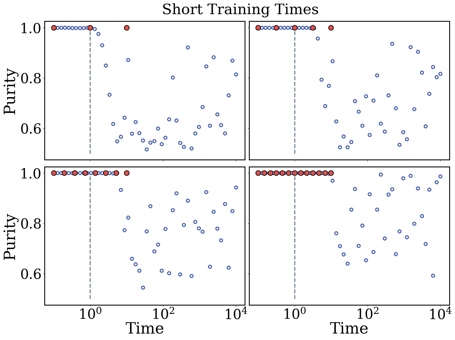
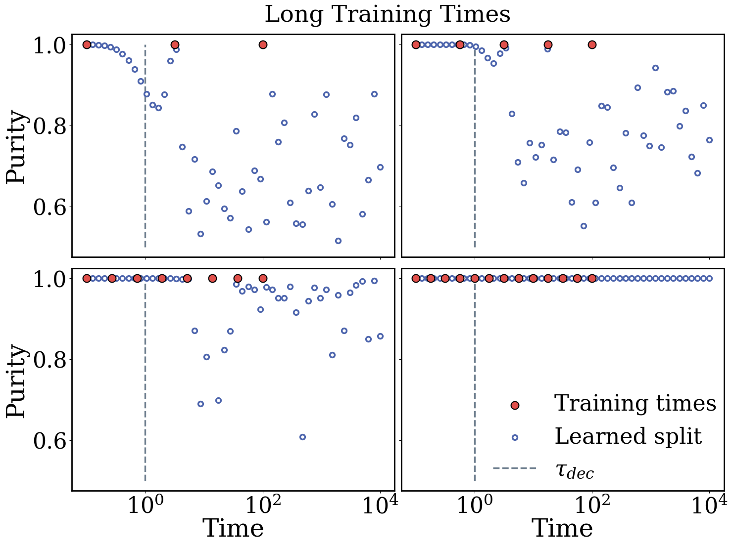
Figure 1: We illustrate the impact of different arrays of training times (solid red markers) on the full behavior of the solution found by our algorithm (open blue markers). For sets that extend sufficiently beyond the decoherence time (dashed line) and which are sufficiently dense, a well-behaved solution is found with unit purity (of the reduced density matrix) extending to late times (lower-rightmost panel). In other cases solutions are found which fluctuate away from the desired pure evolution in a variety of ways (other panels). The red training markers are separated by time $\Delta t$ and run to a maximum value $T_{\rm train}$ as per Eq. (10).

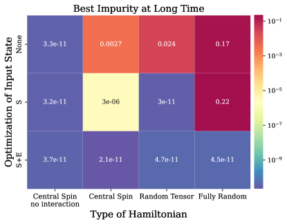
Figure 2: Best late time linear entropy achieved by the different optimization methods for various Hamiltonians. The columns correspond to the Hamiltonians described in Sec. IV.2. The rows correspond to the different initial state optimizations from Sec. IV.1; the unitary $B$ is optimized in each case.

IV Results

We numerically searched for factorizations using a number of different schemes. Each scheme draws from one of three approaches to initial conditions, and one of four types of Hamiltonian. In this section we present these technical findings. In what follows, it is important to remember that there are two factorizations of the Hilbert space that one must keep track of: the “fiducial” factorization, $\mathcal{H_{\sigma}}\otimes\mathcal{H_{\epsilon}}$ in which the Hamiltonian is first supplied, and the “destination” $\mathcal{H}_{s}\otimes\mathcal{H}_{e}$ which is the one our algorithm lands on. The two are related by the unitary $B$ as in Eq. (4).

IV.1 Approaches to initial conditions

While we are interested in finding the optimal factorization, parameterized by the unitary $B$, our cost, Eq. (10), is a function of both $B$ and the initial state $|\psi(0)\rangle_{w}$. Thus, while we always optimize over $B$, we explore various levels of optimizing the initial state which we outline below in increasing order of complexity.

No initial state optimization,

Here we fix our initial state to be a product state in the fiducial basis $|\psi(0)\rangle_{w}=|\xi\rangle_{\sigma}|\phi\rangle_{\epsilon}$ and optimize over just the factorization parameterized by $B$. This case corresponds to asking whether a set of dynamics, with a particular initial condition, can be viewed as corresponding to two approximately well-defined subsystems.

System state optimization.

In addition to optimizing over $B$, we also optimize over the initial state in the fiducial system Hilbert space, $\mathcal{H}_{\sigma}$, i.e. $|\psi(0)\rangle_{w}=A_{\sigma}\otimes 1_{\epsilon}(|\xi\rangle_{\sigma}|\phi\rangle_{\epsilon})$ where $A_{\sigma}\in U(d_{s})$ is to be optimized. This is typically the case encountered in the lab: the experimentalist can set the state of the system being studied, for example the spin of an electron, and not of the more disordered environment with which it interacts.

However, in the case of cosmology, it is not clear what such a bipartite factorization should look like. For example, in order to study the decoherence of the curvature perturbations that are setup during the inflationary epoch, some have defined the modes that leave the Hubble horizon (i.e. the ones that leave observable imprints on large-scale structure) as the “system” while modes that stay within the Hubble horizon as the “environment”, though this choice remains arbitrary [24, 25, 26, 27, 28]. One approach might be to make choices that reflect only quantities within the limits of what we actually measure, but the Universe as we usually model it behaves very classically even well outside those limits. Still, those limits are steadily receding in the face of new astronomical observations and new quantum phenomena, such as non-gaussianity or entanglement [29], could emerge as the new data comes in.

Global state optimization.

In this approach, in addition to optimizing over the factorization parameterized by $B$, we optimize the global initial state, i.e $|\psi(0)\rangle_{w}=A_{w}|\xi\rangle_{\sigma}|\phi\rangle_{\epsilon}$ where $A_{w}\in U(d_{w})$. By allowing ourselves freedom in the global initial state we can stay oblivious to any prior notion of a working basis and, in cases where a notion of a system-environment factorization is not defined a priori, allow us to define the factorization in which a random initial system state decoheres.

IV.2 Hamiltonians considered

The existence of a subsytem description depends on the dynamics governing the evolution of the global state. The discussion of the sort of dynamics that enable the existence of pointer states is deferred to Section IV.4; here we merely state our trial Hamiltonians. Note that a particular Hamiltonian is fundamentally characterized by its eigenvalues and any physical description is attributed to the choice of a fiducial factorization.

Central Spin.

Here we imagine that there is a central qubit in $\mathcal{H_{\sigma}}$ that interacts with a bath of environment qubits in $\mathcal{H_{\epsilon}}$, where the interaction with each environment qubit consists of a single Pauli string, in the presence of an external field. That is,

$$H=\alpha\sigma^{(Z)}_{s}+\alpha\sum_{i}^{n_{e}}\sigma_{e_{i}}^{(Z)}+\sum_{i}^{n_{e}}\beta_{i}\sigma_{s}^{(p_{i})}\otimes\sigma_{e_{i}}^{(q_{i})}$$ (12)

where $\sigma^{(.)}\in\{\sigma^{X},\sigma^{Y},\sigma^{Z}\}$ is a single qubit Pauli operator and we have suppressed the identity operators in each term. The central spin model is of interest to us because its parameters can be easily dialed to study various cases that appear in the decoherence literature. For example, setting $\beta_{i}=0$ gives a perfectly decoupled Hamiltonian or, by choosing each $p_{i}$ from $\{X,Y,Z\}$ such that $p_{i}\neq p_{j}$ (for $n_{e}\leq 3$) one can have a simple Hamiltonian which nonetheless contains several non-commuting terms. We ran both of these sub-categories through our algorithm.

Quantum Measurement Limit

This Hamiltonian takes the form $H=H_{\sigma}\otimes H_{\epsilon}$ in the fiducial factorization where $H_{\sigma/\epsilon}$ are random (traceless) Hermitian matrices. We use the term “quantum measurement limit” here, although the tensor product form is actually a (commonly studied) special case of this limit (which is discussed in more generality in [30])

Random Hamiltonian.

In this case $H_{w}$ is a randomly generated Hermitian matrix.

IV.3 Results for each of the twelve combinations of the above

We ran the four Hamiltonians in Sec. IV.2, for each of the three approaches to initial conditions in Sec. IV.1, $\mathcal{O}(100)$ times to explore the solution space obtained by our algorithm. For each iteration, we generate a starting guess randomly for the unitaries $B$ and $A$ (where applicable), as well as generating a new Hamiltonian for the random Hamiltonian and quantum measurement limit cases. We summarize our results in the tile plot of Fig. 2 where we select the run achieving the lowest cost in the late time limit for each of the categories. We take this late-time limit to be $t\approx 10^{5.5}$ due to numerical considerations (as discussed in Appendix C). Let us understand these statistics row-by-row.

The top row of Fig. 2 shows results for the case where there is no optimization over the unitary $A$ (defined only in the system and global state optimization cases). For that case the algorithm can find a satisfactorily low cost for only the decoupled Hamiltonian where any unitary of the form $B=B_{\sigma}\otimes B_{\epsilon}$ will form a solution (although this does not imply that all solutions to $B$ must be tensor products; consider a SWAP gate for a trivial counter-example). Unsurprisingly, we do not get low cost solutions for the other Hamiltonians with this initialization approach; even though the cost is $\mathcal{O}(10^{-4})$ for the non-commuting central spin (second column), the solution does not generalize to arbitrary times (i.e. other than the ones on which it was trained). While not shown here, this non-generalizability can be seen in Fig. 7 in Appendix C.

In the second row, we additionally find generalizable solutions to the random tensor Hamiltonian. This is because, for $H=H_{\sigma}\otimes H_{\epsilon}$, the cost vanishes when $B$ is any tensor product unitary and $A_{\sigma}|\xi\rangle_{\sigma}=|s_{i}\rangle_{\sigma}$, where $|s_{i}\rangle_{\sigma}$ is an eigenstate of $H_{s}$. The non-commuting central spin has an even lower cost than in the top row because there is more freedom in choosing the global initial state but this is still not sufficient to generate a solution that generalizes to arbitrary times.

Finally, the last row shows results for the case when we optimize over the global initial state. In this case, the algorithm is successful in finding generalizable solutions to all categories of Hamiltonians. There is a wide variety of solutions, each with a different physics interpretation, that are available to the algorithm in this scenario; we elaborate more on the details of this solution space in Sec. IV.4.

While Fig. 2 only shows the most optimal solution, the detailed statistics for each class of Hamiltonians is discussed in Appendix C and Fig. 7 therein.

IV.4 Analysis

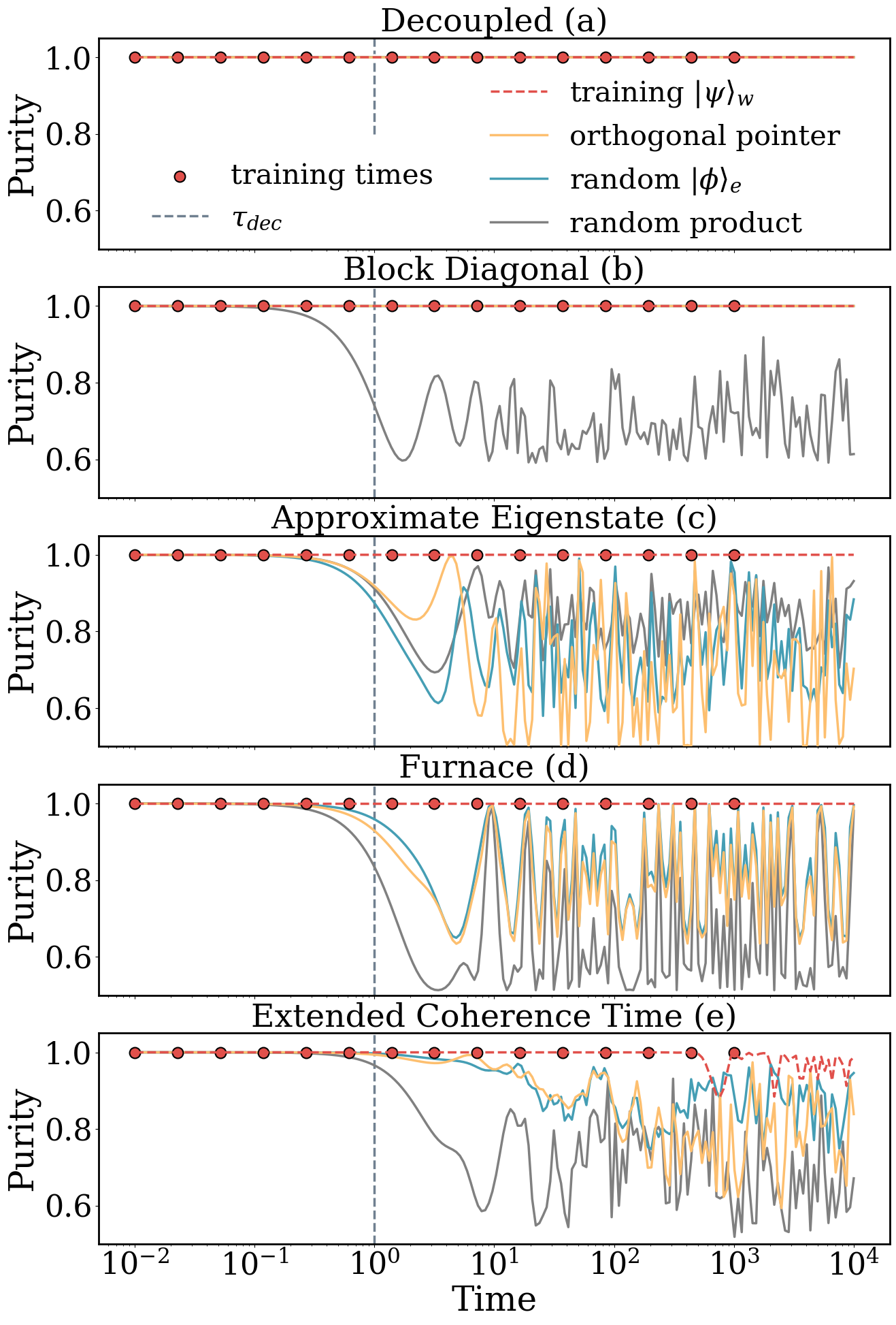
Figure 3: Time evolution of the purity of the reduced system density matrix for each of the categories of the “destination” Hamiltonians identified by our algorithm, as discussed in Sec. IV.4. When the purity is close to one, the training state is separable, i.e. $|\psi\rangle_{w}=|\chi\rangle_{s}|\phi_{e}\rangle$ in the destination factorization. Thus, we also show the effect on the purity resulting from substituting the system state for the orthogonal state, $|\chi\rangle_{s}\rightarrow|\chi^{\prime}\rangle_{s}$, and of randomizing the environment state $|\phi\rangle_{e}$. While in the decoupled case all initial product states remain unentangled for arbitrary times, the other destinations only allow very particular states to stay unentangled beyond the decoherence time. The furnace case is peculiar in that it admits a pointer state only for particular choices of the environment state, as elaborated on in Fig. 5.

There are a plethora of solutions that can satisfy the problem of identifying subsystems as we have posed it here (i.e. by the vanishing of the cost Eq. (9)). Below, we outline these categories and elaborate on the characteristics of each of the class of solutions. We are particularly interested in the dynamics that enable the existence of pointer states and here we adopt the “Heisenberg picture” where we study the Hamiltonian in the new factorization. The properties exhibited by these various “destination” Hamiltonians can also be inferred from the evolution of different kinds of initial states as shown in Fig. 3. In this section we discuss each type of destination Hamiltonian in turn, enumerated in order of the corresponding panel in Fig. 3

(a) Decoupled Hamiltonian.

Here the Hamiltonian takes the form,

$$H=H_{s}\otimes\mathbb{1}_{e}+\mathbb{1}_{s}\otimes H_{e}$$ (13)

so that the system and environment are totally decoupled. In this case, the entropy of the initial state remains constant and an initial product state remains unentangled. However, this is a vanishingly rare solution that is not expected for random Hamiltonians. This can be understood heuristically by a simple degrees-of-freedom counting argument: decomposing a generic Hamiltonian in the Pauli basis gives a total of $4^{n_{w}}$ terms (where $n_{w}$ is the total number of qubits) which can be arranged in a matrix of Pauli coefficients of dimensions ($4^{n_{s}}$, $4^{n_{e}}$) in such a way that the first column and row correspond to the system and environment self-interaction terms respectively. Thus, there are a total of $4^{n_{s}}-1$ terms that contribute to the system self-interaction and $4^{n_{e}}-1$ for the environment (the $-1$ occurs because there is a Pauli coefficient for the identity which only contributes a global phase and is not of physical significance). The rest of the $4^{n_{s}+n_{e}}-4^{n_{s}}-4^{n_{e}}+1$ terms contribute to the interaction Hamiltonian, $H_{\rm int}$. Thus, say for a 3-qubit world, expecting to find a factorization where the Hamiltonian is decoupled amounts to the expectation that the $45$ interaction coefficients can be regrouped into $20$ slots for the self-interaction terms .

It turns out that the algorithm finds this solution for the (interacting) central spin model. This may initially seem surprising, however, in fact this model passes the counting argument since, in the fiducial factorization, $H_{\rm int}$ contains only $n_{e}$ non-zero Pauli terms. We depict the result of evolving several product states in this decoupled factorization of the central spin model in Fig. 3; clearly they all remain product states throughout the evolution.

The transformation of an interacting Hamiltonian to a decoupled one is familiar from bosonization of interacting field theories [32, 33] or the Jordan-Wigner (JW) transformation. The latter is particularly pertinent for our central spin Hamiltonian since, for several classes of Hamiltonians that are quadratic in the spin operators, the JW transformation unitarily transforms the spin system to a set of free fermions [34, 35]. We comment on the interpretation of such non-local transformations in Section V. Some authors have argued that factorizations with quasi-classical subsystems can be identified as those that minimize the interaction Hamiltonian [3, 6]. While this decoupled case certainly passes that criterion, the requirement seems too restrictive. In the rest of this section, we show several destination Hamiltonians that admit pointer states, and thus a notion of quasi-classicality, despite having significant interactions between the subsystems. We refer the reader to Ref. [36] for an implementation of a quantum algorithm that can be used to search for factorizations in which the Hamiltonian is decoupled.

In looking at the second column of Fig. 2, one might wonder why, if such a decoupled Hamiltonian can be found for the central spin, the cost in the top row is considerably higher than in the bottom row. This is because, as mentioned in Sec. III, our initial state is a product state in the fiducial factorization where the Hamiltonian in Eq. (12) has interactions. Though there exists a unitary such that $BHB^{\dagger}$ is decoupled (the destination TPS), the algorithm has no direct knowledge of this fact. Instead, it is tasked with minimizing the cost Eq. (10) (in the Schrödinger picture). But since $B|\xi\rangle_{s}|\phi\rangle_{\epsilon}$ is entangled, without initial state optimization the algorithm is unable to access a product initial state in the destination TPS, which is required to achieve a low cost for the decoupled destination Hamiltonian. When we include initial state optimization (last row of Fig. 2) then, as expected, the algorithm succeeds in finding this solution. And not surprisingly the middle row, showing the partially optimized case, reflects a cost midway between the two extremes.

(b) Block Diagonal Hamiltonian.

For any Hamiltonian, there always exists a factorization, defined by the eigenstates of the Hamiltonian, that admits pointer states. Specifically, we show in Appendix A that for any Hamiltonian there always exists a factorization of the Hilbert space where the eigenstates are separable so that it may be written in the form

$$H=\sum_{i}|\chi_{i}\rangle\langle\chi_{i}|_{s}\otimes H_{e}^{(i)}$$ (14)

It is straightforward to verify, as shown in Appendix A, that $|\chi_{i}\rangle_{s}$ are the pointer states and that a generic state will evolve into a state whose system density matrix is diagonal in the pointer basis, i.e.

$$\rho_{s}\xrightarrow{U_{t}}\rho_{s}\approx\sum_{i}p_{i}(t)|\chi_{i}\rangle\langle\chi_{i}|_{s}$$ (15)

(for a sufficiently large and scrambling environment) as is characteristic of einselection. It is also manifest from the form of Eq. (14) that $H$ is block diagonal in the pointer basis and, furthermore, that the $|\chi_{i}\rangle_{s}$ are robust to entanglement independent of the choice of the environment state or the size or scrambling nature of the environment. This feature can be seen in Fig. 3 where we show that randomizing the environment state does not degrade the purity of the reduced density matrix. We also note that the pointer states are stationary, while an arbitrary environment state will evolve under the evolution generated by the $H_{e}^{(i)}$ operators. All these properties, as well as a general recipe for finding this factorization for an arbitrary Hamiltonian, are proved in Appendix A.

Such a mapping to a factorization where the energy eigenstates are separable has some similarity with the case of dynamical decoupling in superconducting qubits (see e.g. Appendix A in [37] for an overview) . There, the “logical” qubits (what we call the “destination” TPS) correspond to the energy eigenstates of a world described by interacting “physical” qubits (what we have called the “fiducial” TPS). Defining the logical qubits in this way can mitigate certain sources of noise[38].

In the decoherence literature authors often consider special Hamiltonians; such as those for which the system self-interaction commutes with the interaction, $[H_{s}\otimes 1_{e},H_{\rm int}]=0$ or a “quantum measurement limit” where the Hamiltonian is dominated by a single interaction term $H\approx H_{s}\otimes H_{e}$. These are both special cases of the more general block-diagonalization procedure outlined above where the $H_{e}^{(j)}$ operators in Eq. (14) have specific relationships. For example, in the quantum measurement limit all the $H_{e}^{(i)}$ operators are the same up to an overall scaling, $H_{e}^{(j)}\propto H_{e}^{(i)}$. A particularly interesting sub-case of the block diagonal Hamiltonian is when there exists a decoherence-free subspace (DFS) (a topic relevant for quantum computing [39, 40]). In this factorization some, but not all, eigenvectors have vanishing entropy and, as in the quantum measurement limit, their corresponding $H_{e}^{(i)}$ operators are proportional to each other. Writing out the Hamiltonian in the global eigenbasis, we can interpret it as a sum of a decoupled (i.e. DFS) and an entangling part:

$$\begin{gathered}H=\sum_{i}^{n_{w}}|i\rangle\langle i|_{w}\lambda_{i}=\sum_{i\in C_{\rm DFS}}|i\rangle\langle i|_{w}\lambda_{i}+\sum_{i\in C_{\rm rem}}|i\rangle\langle i|_{w}\lambda_{i}\\ \\ =H_{\rm DFS}+H_{\rm rem}\,.\end{gathered}$$ (16)

Here we have split up the eigendecomposition into a term containing only the zero entropy eigenvectors (labeled ‘DFS’) and a term containing the remainder (labeled ‘rem’). Thus, the disjoint set of indices satisfy the condition $C_{\rm DFS}\cup C_{\rm rem}=\{1,...,d_{w}\}$ and the operators $H_{\rm DFS}$ and $H_{\rm rem}$ are partial-rank. Now the reduced density matrix of any state composed of only the zero entropy eigenstates,

$$|\psi\rangle=\sum_{i\in C_{\rm DFS}}\alpha_{i}|i\rangle_{w}$$ (17)

will have constant purity (which may be vanishing for certain choices of $\alpha_{i}$) and have evolution generated under $H_{\rm DFS}$.

Such a DFS solution lies in the intermediate regime of the general block diagonal form in Eq. (14) and the decoupled Hamiltonian in Eq. (13). Since $H_{\rm DFS}$ is subject to the same constraints as those for the (fully) decoupled Hamiltonian (see footnote 7), we do not expect to find such a factorization for random Hamiltonians. However, the central spin model admits both the decoupled and the block diagonal destinations, and in that case our algorithm is indeed able to find this intermediate DFS solution.

(c) Approximate Eigenstates.

This class of solutions is particularly interesting because it exhibits dynamic pointer states, though it fails to provide a sufficiently distinguishable basis of such states. Here, there is a dominant contribution to $|\psi\rangle_{w}$ from a low entropy energy eigenstate and smaller but, crucially, non-negligible contributions from high entropy eigenstates. More precisely, in the language of Appendix A, the world energy eigenstates are of the form,

$$|1\rangle_{w}=|1\rangle_{s}|1\rangle_{e}$$ (18)

$$|i\rangle_{w}=\sum_{j}^{d_{s}}\beta_{j}^{(i)}|j^{(i)}\rangle_{s}|j^{(i)}\rangle_{e}$$

where the Schmidt coefficients $\beta_{j}^{(i)}$ are not all zero for $j>1$ $\forall i\in\{2,..,d_{w}\}$ (for convenience we choose to label the low entropy eigenstate $|1\rangle_{w}$). And the global state is of the form,

$$\begin{gathered}|\psi\rangle_{w}=\sum_{i=1}^{d_{w}}\alpha_{i}|i\rangle_{w}\\ \textrm{such that }\alpha_{1}\gg\ \alpha_{j}\textrm{ for }j>1.\end{gathered}$$ (19)

This decomposition of $|\psi\rangle_{w}$ into eigenstates $|i\rangle_{w}$ and their corresponding linear entropy of entanglement, Eq. (6), is shown in Fig. 4 for a world with one system and two environment qubits. We note that the correlation between the entropy and $|\alpha_{i}|^{2}$ for $i>2$ seems typical of these ‘approximate eigenstate’ solutions but that it is likely a feature of the search algorithm and not of inherent physical significance. We have checked numerically that, as long as the condition $\alpha_{1}\gg\alpha_{j>1}$ is satisfied, there is considerable freedom in distributing the weights amongst the other higher entropy eigenstates. In Fig. 3 c. we show the evolution of the purity of the redcued system density matrix of such a state (labeled ‘training $|\psi\rangle_{w}$’) compared to other states.

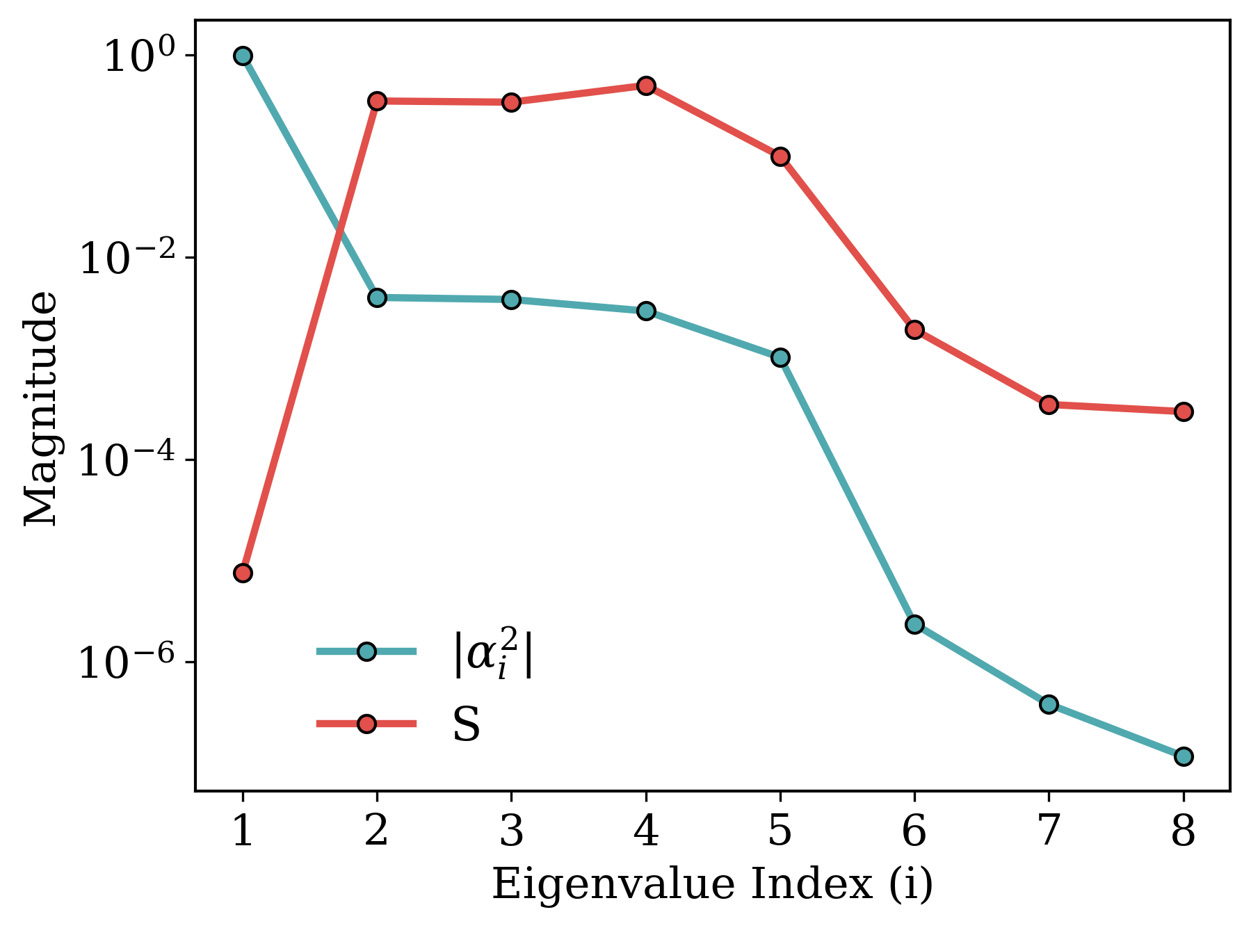
Figure 4: The decomposition of $|\psi\rangle_{w}$ in the energy eigenbasis for the case of the ‘approximate eigenstate” solutions discussed in Sec. IV.4 (see Eq. (19)) is shown in blue along with their corresponding linear entropy of each energy eigenstate (defined in Eq. (6)). These solutions are dominated by a single low entropy energy eigenstate, although high entropy eigenstates contribute to a small degree. The plot is arranged in order of decreasing $|\alpha_{i}|$.

The fact that the contribution to $|\psi\rangle_{w}$ from the high entropy eigenstates is small, but not negligible, is crucial as it leads to a pure $\rho_{s}$ for times several orders of magnitude greater than the decoherence time (see Fig. 3 c.), while allowing the state to be dynamic. These two behaviors resonate with our classical experience of subsystems. It appears, at first, that such solutions are exactly the ones that the author of [3] is in search of, i.e. those that have a high degree of predictability (as evidenced by the purity of the system state) as well as “autonomy” (that their dynamics are not trivial). However, while this class of solutions satisfactorily minimizes our cost function (Eq. (10)), it is not clear how to apply the decoherence framework to it since we do not have a multi-dimensional distinguishable basis of states of the form in Eq. (19). This should be contrasted with the TPS that leads to a block diagonal Hamiltonian in the pointer basis (c.f. part (b)) where we do have a complete pointer basis (such that the system density matrix follows Eq. (15)) but that the pointer states remain static.

(d) Furnace Hamiltonian.

In this scenario there exist pointer states when the environment state exists in a particular subspace of $\mathcal{H}_{e}$. Specifically, suppose

$$H=\sum_{i}^{d_{e}}H_{s}^{(i)}\otimes|i\rangle\langle i|_{e}$$ (20)

and pick, for simplicity, two particular but arbitrary indices $p$, $q$ such that $[H_{s}^{p},H_{s}^{q}]=0$ . Then, any initial state of the form $|\psi\rangle=|s_{i}\rangle(\alpha|p\rangle_{e}+\beta|q\rangle_{e})$ (where $|s_{i}\rangle$ is a mutual eigenstate of $H_{s}^{p/q}$) will remain unentangled. Of course, while we picked just two commuting $H_{s}^{(i)}$ terms for simplicity, the argument is quite general; all that is needed is for the environment state to project the total state into a subspace that admits a pointer state solution.

The form of the Hamiltonian in Eq. (20) also makes it clear that, for a fixed system size, the larger the environment the more such solutions will exist. This is because there are $d_{e}$ terms and if each of the $H_{s}^{(i)}$ operators is generated randomly the likelihood that any two operators will commute (or approximately commute) increases. As shown in Fig. 3 d., clearly the trained state remains unentangled throughout the evolution while the other states, including the state made from randomizing the environment state, generally do not. Although in this figure the ‘furnace’ solution appears to resemble the ‘approximate eigenstate’ solution, the distinguishing feature can be seen in Fig. 5 which shows that the purity of the reduced density matrix of the trained state is robust to arbitrary changes within a particular subspace.

Intuitively, this solution can be understood in the following physical sense: consider a pendulum in the lab that undergoes constant environment monitoring and thus stays in the pointer state as it oscillates (as is expected of a subsystem). But now the lab assistant turns up the temperature of the room, as in a furnace, so that the pendulum incinerates and its atoms are dispersed amongst the various degrees of freedom available in the room. Here, though the Hamiltonian has remained the same, changing the environment state has drastically altered the description of the system to one that no longer has a pointer state.

(e) Extended coherence time.

These solutions sustain a moderately high purity for $1-2$ orders of magnitude longer than the typical decoherence time. From the algorithm’s perspective such solutions can be thought of as a result of poor training or poor generalizability. In the former case, the algorithm finds a combination of initial state and factorization such that the solution only roughly approximates one of the other “perfect” solutions above. However, the convergence to such a solution is slow and the algorithm hits a time-wall before it can get sufficiently close to such a solution. Poor generalizability occurs when the algorithm is able to sufficiently minimize the cost for the training steps, but that the solution does not generalize well beyond those finite times. In this case, the situation resembles the purity plots shown in the left panel of Fig. 1. As mentioned in Section III, since we take our maximum training time to be $\approx 10^{2}t_{\rm dec}$, it makes sense that the failure to generalize manifests beyond this domain.

Such ‘extended coherence time’ solutions also occur in the case of fixed input state optimization (i.e. $A=\mathbb{1}$). This is because, in fixing $A$, the algorithm loses control over the degrees of freedom required to sufficiently minimize the cost and to ensure that the purity of the reduced density matrix remains high for times much greater than $t_{\rm dec}$. We find these solutions for all classes of Hamiltonians and they may be interpreted as short-lived subsystems. That is, as a set of dynamics which, a priori, appears highly entangling but can be viewed in another factorization as temporarily pertaining to subsystems. Ultimately, we lack an analytic understanding of these solutions and caution from reading too much into the numerics shown here. Firstly, the purities obtained in this case are substantially lower than in the case where we optimise over the initial state (see the right panel of Fig. 8). Secondly, it is unclear how these solutions generalize to larger systems. Thus, rather than highlighting new physics, perhaps the fleeting subsystems found here are akin to shapes found in the sky when cloud watching. On the other hand, these solutions might most closely reflect the fate of all subsystems in a dark energy dominated universe.

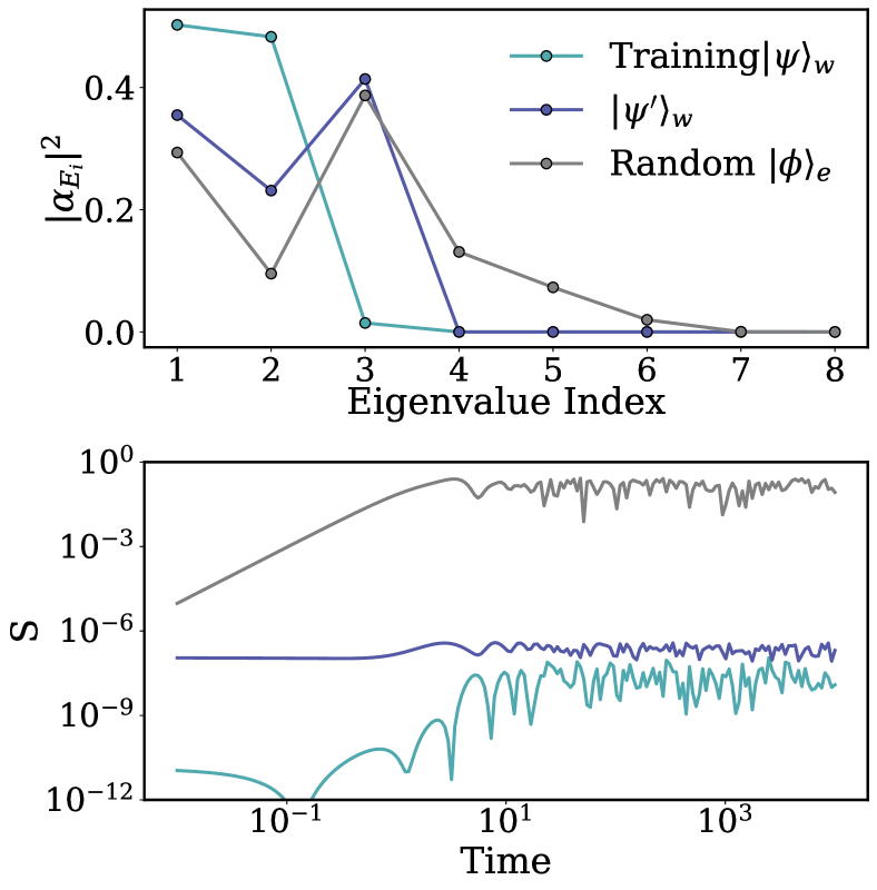
Figure 5: In the furnace Hamiltonian, a pointer state for the system exists only if the environment is in a particular subspace of $\mathcal{H}_{e}$ (unlike the Block diagonal case, c.f. Fig. 3b, where the pointer state is indifferent to the choice of $|\phi\rangle_{e}$). Here we depict this phenomenon by perturbing the trained state $|\psi\rangle_{w}$ (turquoise) such that the new state $|\psi^{\prime}\rangle_{w}$ (purple) has support from the same energy eigenvectors as those that contribute to the trained state (top panel). The bottom panel verifies that such a state indeed remains a product state at late times. Note that $|\psi\rangle$ and $|\psi^{\prime}\rangle$ share the same system state in $\mathcal{H}_{s}$ (up to an overall phase). We show, for comparison, another state where $|\phi\rangle_{e}$ is randomized leading to a large increase in the linear entropy in the typical decoherence time (the furnace “incinerates” in the analogy of the text in Section IV.4(d)).

V Many more worlds

Everett’s relative state interpretation of quantum mechanics [41, 42, 43] was meant to address the system-observer dichotomy, where the observer/apparatus is treated as a classical object (and many textbooks continue to present this dichotomous exposition). The relative state interpretation, and its various extensions in the many-minds, de Witt’s many-worlds [44], or Zurek’s existential [17] interpretations, posits a global wave function that evolves unitarily and definite perceived outcomes result from the state of the observer becoming correlated with the state of the system. It is in this sense that the relative state interpretation may be thought of as a literal reading of unitary quantum mechanics. For concreteness, consider a system in the state

$$|\psi\rangle_{s}=\frac{1}{\sqrt{2}}(|0\rangle+|1\rangle)$$ (21)

that interacts with an apparatus such that

$$\frac{1}{\sqrt{2}}(|0\rangle+|1\rangle)|a_{r}\rangle\xrightarrow{U_{t}}|\Psi_{f}\rangle=\frac{1}{\sqrt{2}}(|0\rangle|a_{0}\rangle+|1\rangle|a_{1}\rangle)$$ (22)

where $|a_{r}\rangle$ is the “ready” state of the apparatus. The relative state interpretation posits that no definite state can be ascribed to the system or the apparatus but, instead, the state of the apparatus (or the observer), say $|a_{1}\rangle$, should be understood as being correlated with the state $|1\rangle$ of the system. Then, each of the two terms of Eq. (22) correspond to the two “branches” of the wave-function. But why should the branches be described by the particular choice of basis used in Eq. (22)? Consider instead the system and apparatus bases,

$$|\pm\rangle_{s}=\frac{1}{\sqrt{2}}(|0\rangle\pm|1\rangle)\textrm{ and }|a_{\pm}\rangle=\frac{1}{\sqrt{2}}(|a_{0}\rangle\pm|a_{1}\rangle);,$$

so that the final global state in Eq 22 takes the form,

$$|\Psi_{f}\rangle=\frac{1}{\sqrt{2}}(|+\rangle|a_{+}\rangle+|-\rangle|a_{-}\rangle)\;.$$ (23)

This ambiguity in the choice of basis between Eq. (22) and Eq. (23) poses the questions: what exactly has the apparatus “measured”? In the language of the many worlds interpretation, which basis (that of Eq. (22) or 23) describes the post-measurement world? Einselection resolves this preferred basis problem [10] by considering the interaction of the apparatus with the environment which, depending on the details of the Hamiltonian, singles out a set of preferred basis so that it is, say, the $\{a_{0},a_{1}\}$ basis that remains robust to entanglement with the environment and that the state of the system should be inferred relative to this basis [12].

Thus, einselection provides a way to dynamically select the preferred basis of the subsystems. However, the presence of pointer states is crucial and requires specially constructed Hamiltonians (whether through the predictability sieve strategy [23] or by virtue of vanishing commutators in the self and interaction Hamiltonians [12]). In particular, it requires one to specify the individual subsystems that the Hamiltonian describes.

In this paper we set out to answer the question if the division into subsystems can be derived, as opposed to assumed, from the spectrum of the Hamiltonian. In Section IV.4, we have shown that there always exists at least one such factorization – that in which the global eigenbasis is separable, that admits pointer states and hence can exhibit einselection (in the sense of Eq. 22 above) and that for “real-world” Hamiltonians, several other choices also exist. But this introduces a new issue: the block diagonal factorization is available in addition to the other factorizations that also support einselection (such as the coherent state wavepackets of the ACL model discussed in Section II). What then favors one factorization over the other? We stumble upon a “global” analog of the preferred basis problem: if multiple TPS admit decoherent histories why should the world branch in one factorization over the other? Why should the physicist’s choice of global basis in writing down the state determine the branches of the worlds? Moreover, the resulting ambiguity is in a sense more unsettling than the preferred basis ambiguity of the system subspace. The various choices of TPS describe many “realms”: the set of worlds described by the fiducial factorization have a different ontology than the set of worlds in the realm described by the destination factorization. The harmonic oscillator of the ACL is far from an SHO in a different system-environment split. And while both realms share the same global energy spectrum, the scene described by a central spin surrounded by environment qubits in an external magnetic field is radically different than the fermionic degrees of freedom with hopping terms obtained by taking a Jordan-Wigner transform. Note also that all these realms exist at fixed system and environment size, which has been the focus of this work. Allowing additional freedom in the sizes of the individual Hilbert space factors, which in principle is unobjectionable for the global state since two Hilbert spaces of the same dimensions are isomorphic, will only add to the diversity of the realms. Furthermore, while we have focused on only bipartite factorizations, the case of multipartite subsystems may further add to this diversity, especially if one considers $\dim{(\mathcal{H}_{w})}$ to be highly factorizable as appears to be the case for our Universe [46].

This ontological ambiguity between the realms is unsettling but, while the authors of [47, 2] refer to the “physical” factorizations describing “real” and the other factorizations as “virtual” subsystems, we reserve judgment on the “reality” of eccentric realms . One might argue that the “physical” factorizations have some notion of locality either in the pointer state as in [2, 5], at the level of the Hamiltonian [4], or in the set of observables [1]. While there is some merit to this argument, we remain curious if the “local” factorizations are in some deeper sense preferred over the other ones and whether one can derive this preference from something fundamental rather than inflicting this classical prejudice onto the Hilbert space. Assuming locality is principally not much different than assuming a particular factorization of the Hamiltonian as is done implicitly in most formulations, and explicitly in Wallace’s three postulates [48, Chapter 1], of QM.

Similar prejudices enter into arguments that try to minimize $H_{\rm int}$ in an effort to look for a preferred factorization [3, 6]. But there is nothing in the einselection formalism (or the relative state interpretations) that presupposes a TPS that minimizes the interaction Hamiltonian. Attempts to search for such a preferred TPS by minimizing the interaction strength are misguided because important physical cases are described by a dominant $H_{\rm int}$ term and in those cases einselection occurs not inspite of but because of the strong interaction (see Quantum Measurement Limit in Section IV.2).

While others have put forth “in-principle” algorithms to search for quasi-classical factorizations [5, 7], we have been successful in practically implementing an algorithm to explore the many realms that coexist in worlds with a given global energy spectrum. What remains missing is some measure on the space of these realms serving much the same purpose as that served by the predictability sieve for the preferred basis problem, or by the Born rule for the many world branches (to suppress the “maverick” worlds [49]). As we explain in Appendix B, one such measure is induced by our algorithm based on the minimization of the cost Eq. (10). However it is unlikely that such a measure is of any physical significance.

The abundance of coexisting realms, and the absence of a physical measure to discriminate among them appears to be related to issues that have been explored in the context of the consistent histories formalism, where alternative sets of complete projectors lead to different coexisting narratives [50, 51, 52, 53] (“alternate facts”, in the language of [54]). However, those discussions typically do not explore as wide a range of tensor product structures as we consider in this paper.

The discussion in this section has taken a predominantly “cosmological” point of view, where care is taken not to refer to an external observer. From that point of view one can wonder if there ought to be some physical principle that allows us to choose a “correct” realm from the many offered up by the formalism. We note that one could instead take an “engineering” perspective and think of the systems we explore in this paper as actual sets of qubits sitting in the laboratory. In that case it is clear that each of the coexisting einselecting realms we’ve identified are equally physical, and could in fact be relevant to us if we are able to develop probes (from our larger world or just from another laboratory system of qubits) that can interact with the particular subsystem in question. We are intrigued by the sharp contrast this engineering perspective makes in comparison to the cosmological one.

VI Conclusions

In this work we have addressed the question: “Given a quantum world, determined by its energy spectrum, can we find factorizations of the global Hilbert space such that certain states of the system are robust to entanglement?”. The dynamical selection of such robust (pointer) states, known as einselection, has a key role in the emergence of classical from quantum allowing systems in pointer states to be tracked classically without consideration of various quantum processes. We have explored this question by constructing a cost function that is sensitive to the purity of the evolving subsystem quantum state. This gives us an operational tool to identify pointer states which we use to numerically explore systems comprised of several qubits. We support our numerical explorations with an analytic discussion of the various behaviors identified.

For a given global Hamiltonian (selected from one of four classes) we utilized a variety of optimization schemes for exploring possible tensor product structures and initial states. We have found that in all cases multiple tensor product structures can be found describing coexisting “realms” that exhibit features of classicality. This was so even for cases with randomly generated energy eigenvalues, and cases with a more structured energy spectrum allowed for a greater variety of classical behaviors. We note that the interactions in these quasi-classical realms need not be weak or local.

We have explored a variety of implications of our results. From a foundational point of view, our results compound interpretational questions that arise when multiple classical worlds coexist within a single quantum description of the Universe. At a more practical level, our results also hint towards new strategies for developing noise robust quantum technologies. The systems we have studied may be viewed as real laboratory objects, with each of the realms having a physical existence which could be examined if suitable probes could be developed. We call out in particular the possible relevance of our results for the engineering of decoherence-free subspaces.

We have not attached a lot of conceptual importance to the fine details of our algorithm (despite the apparent need, in the case of the foundational questions for some sort of measure with which to compare the different realms). However, we are curious if our algorithm (or a related one) might be relevant for practical applications where probes of the qubit systems need to be suitably engineered. In principle the algorithm might reflect some aspects of the engineering process.

VII Acknowledgements

Adil, Albrecht and Sornborger acknowledge support from the U.S. Department of Energy, Office of Science, Office of High Energy Physics QuantISED program under Contract No. KA2401032. ZH acknowledges support from the Sandoz Family Foundation-Monique de Meuron program for Academic Promotion.

A. Adil would like to thank the organizers and participants of the “Foundations Under the Midnight Sun 2023” workshop for several engaging discussions. We thank Lukasz Cincio for help with implementing the numerical algorithm and Michael Hartmann for helpful conversations about the application to superconducting qubits. We also thank M. Lyans for an editorial suggestion and P. Coles for helpful discussions at early stages of this work.

Appendix A Block Diagonal Hamiltonians

All Hamiltonians admit pointer states.

Here we describe how any Hamiltonian may be block-diagonalized to find a factorization that admits pointer states. Very simply, we define the factorization of the world Hilbert space such that the energy eigenstates are separable,

$$|1\rangle_{w}=|1\rangle_{s}|1\rangle_{e}$$

$$|2\rangle_{w}=|1\rangle_{s}|2\rangle_{e}$$

$$|3\rangle_{w}=|2\rangle_{s}|1\rangle_{e}$$

$$\vdots$$

$$|E_{k}\rangle_{w}=|i\rangle_{s}|j\rangle_{e}$$

where $k$ is an index from 1 to $d_{w}$ and $i$ and $j$ run from 1 to $d_{s}$ and $d_{e}$ respectively. Thus, the prescription is a trivial relabelling of the energy eigenstates which allows one to write the Hamiltonian in the following form,

$$H=\sum_{k=1}^{d_{w}}E_{k}|E_{k}\rangle\langle E_{k}| =\sum_{i=1}^{d_{s}}|i\rangle_{s}\langle i|\otimes\sum_{j=1}^{d_{e}}|j\rangle_{e}\langle j|E_{ij}$$ (24)

$$=\sum_{i=1}^{d_{s}}|i\rangle_{s}\langle i|\otimes\tilde{H}_{e}^{(i)}$$

where we have defined $\tilde{H}_{e}^{(i)}=\sum_{j}|j\rangle_{e}\langle j|E_{ij}$.

Recipe to find pointer states.

The argument above shows that any Hamiltonian admits pointer states. However, for a practitioner it might not be clear how one could use that argument to find and prepare pointer states. The claim that one can always find pointer states from this perspective is the claim that it is always possible to find a factorization, parameterized by the unitary $B$, and basis of system states $\{|i\rangle_{s}\}_{i=1}^{d_{s}}$ such that $|\phi(t)\rangle_{w}=Be^{-iHt}|i\rangle_{s}|\psi\rangle_{e}$ remains unentangled for all times. One construction to do so is as follows:

1. The first step is to diagonalize $H$. That is, find an arbitrary unitary $W$ and diagonal matrix $D$ such that $H=WDW^{\dagger}$.

2. The second step is to decompose $D$ into two subsystems. Given a $D$ of the form $D=\sum_{i}\lambda_{i}|i\rangle\langle i|_{w}$ we can introduce a bipartite splitting in the computation basis.
   

   For example, for two qubits we have,

   $$|0\rangle\rightarrow|00\rangle$$ (25)

   $$|1\rangle\rightarrow|01\rangle$$

   $$|2\rangle\rightarrow|10\rangle$$

   $$|3\rangle\rightarrow|11\rangle\,.$$

   Thus we can write $D$ as $D=|0\rangle\langle 0|_{s}\otimes H_{e}^{(0)}+|1\rangle\langle 1|_{s}\otimes H_{e}^{(1)}$ where $H_{e}^{(0)}\mathrel{\mathop{\mathchar 58\relax}}=\lambda_{0}|0\rangle\langle 0|_{e}+\lambda_{1}|1\rangle\langle 1|_{e}$ and $H_{e}^{(1)}\mathrel{\mathop{\mathchar 58\relax}}=\lambda_{2}|0\rangle\langle 0|_{e}+\lambda_{3}|1\rangle\langle 1|_{e}$.
   

3. The states that remain robust to entanglement in the factorization $B=W^{\dagger}$, are given by $W|i\rangle_{s}|\psi\rangle_{e}$ for any environment state $|\psi\rangle_{e}$.

To see that this construction works note that

$$Be^{-iHt}W|i\rangle_{s}|\psi\rangle_{e} =W^{\dagger}We^{-iDt}W^{\dagger}W|i\rangle_{s}|\psi\rangle_{e}$$ (26)

$$=e^{-iDt}|i\rangle_{s}|\psi\rangle_{s}$$

$$=|i\rangle_{s}e^{-iH_{e}^{(i)}t}|\psi\rangle_{e}$$

$$=|i\rangle_{s}|\psi^{(i)}(t)\rangle_{e}$$

where $|\psi(t)\rangle_{e}=e^{-iH_{e}^{(i)}t}|\psi\rangle_{e}$. This state clearly remains unentangled for all times.

Consequences of this construction.

From this form of the Hamiltonian, it is easy to verify some observations. First, that the system states $|j\rangle_{s}$ are pointer states – any initial product state where the system is in a pointer state remains a product state: $|j\rangle_{s}|\phi\rangle_{e}\xrightarrow{U_{t}}|j\rangle_{s}|\phi_{j}(t)\rangle_{e}$ where $|\phi_{j}(t)\rangle_{e}=e^{-i\tilde{H}_{e}^{(j)}t}|\phi_{j}(t)\rangle_{e}$. Note that the system state is not dynamic and, though the environment state evolves in time, the evolution is confined within the subspace of eigenvectors that is projected by the particular choice of pointer state, as shown in Fig. 6.

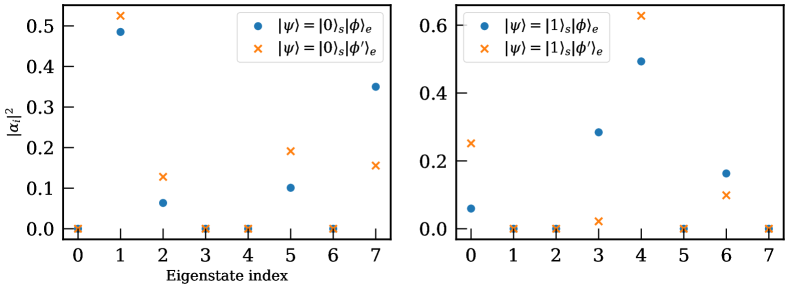
Figure 6: Here we depict the effect of varying the environment state for a particular pointer state in a 1-qubit system and 2-qubit environment world. The figure shows the amplitudes of the coefficients of a product state composed of the pointer state and a random environment state in the energy eigenbasis. As discussed in the text, varying the environment state varies only the components in the subspace of eigenvectors that is projected by the particular choice of pointer state.

Finally, for an arbitrary pure initial state, the reduced system density matrix becomes diagonal in the pointer basis. To see this, start with an arbitrary product state $|\psi(0)\rangle_{w}=\sum_{j}\alpha_{j}|j\rangle_{s}|\phi\rangle_{e}$, (the assumption of an initial product state simplifies the calculation; the argument proceeds similarly for an arbitrary initial state). This evolves as

$$e^{-iHt}|\psi(0)\rangle_{w}=\sum_{j}\alpha_{j}|j\rangle_{s}|\phi_{j}(t)\rangle_{e}$$ (27)

Thus the reduced state on the system is given by

$$\rho_{s}(t)=\sum_{jk}\alpha_{j}\alpha^{*}_{k}|j\rangle\langle k|_{s}c_{jk}(t)$$ (28)

where $c_{jk}(t)=\langle\phi_{k}(t)|\phi_{j}(t)\rangle_{e}$. In the case that the global evolution drives the environment into approximately orthogonal states we have that $c_{jk}(t)\approx\delta_{jk}$ at large $t$ and so the system perfectly decoheres in the pointer basis, i.e.,

$$\rho_{s}(t)\rightarrow\sum_{j}|\alpha_{j}|^{2}|j\rangle\langle j|_{s}\,.$$ (29)

Appendix B Numerical Implementation

The optimization algorithm we employ is commonly used in the tensor network community. Favorable updates of the unitaries $A$ and $B$ with respect to the cost function in Eq. (9) are calculated using common density matrix renormalization group (DMRG) techniques [55] and the so-called Singular Value Decomposition (SVD) “trick”, which is related to finding the closest unitary matrix to a general matrix [56].

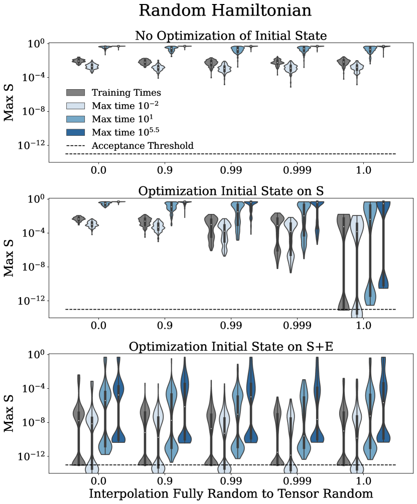
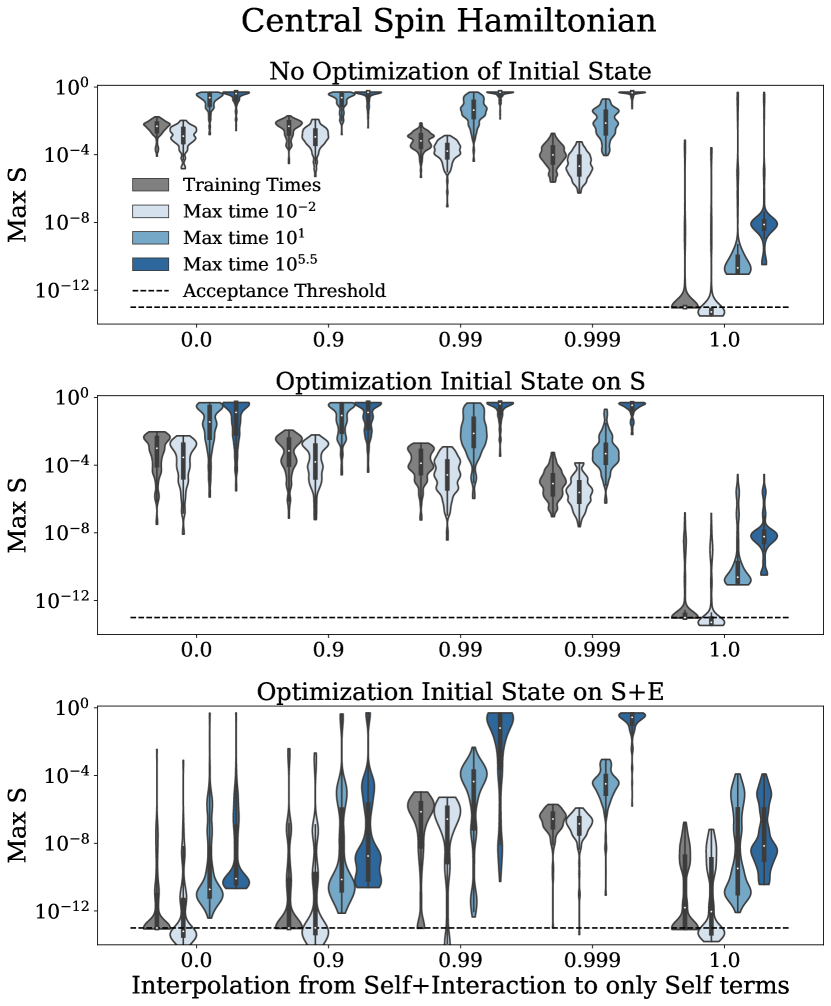
Figure 7: Violin plots capturing the statistics obtained by $100$ random initializations for each case. For each instance, the linear entropy of $\rho_{s}$ is evaluated for the set of training times (grey), as well as a set of times up to a maximum time (different shades of blue), and the highest entropy (i.e. worst-case) point from this set is collected. The various violins then depict the details of the statistics summarized in Fig. 2. Their interpretation is discussed extensively in Appendix C.

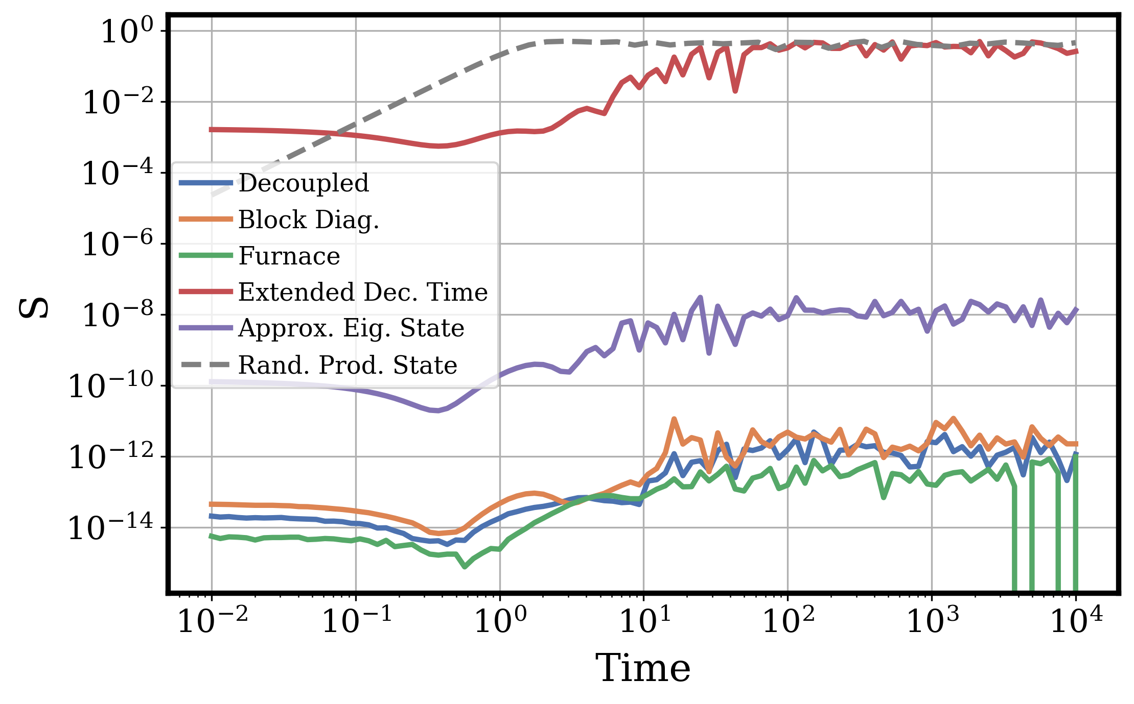
Figure 8: The figure depicts the linear entropy of the trained state (solid colors) for all of the classes of solutions discussed in Sec. IV.4. For comparison, we also show the evolution of the linear entropy of a random product state (dashed) in the fiducial factorization. All the solutions were obtained from the same fiducial Hamiltonian, the central spin (discussed in Sec. IV.2), with one central and three environment qubits. This figure describes the “quality” of each of the solutions (i.e. the depth of the minimum on which the algorithm converges) and should be compared with the last row of Fig. 7.

To demonstrate the approach, assume a hypothetical cost function $\tilde{C}=1-\langle\psi_{1}|U_{1}U_{2}|\psi_{2}\rangle$ with fixed states $\psi_{1},\psi_{2}$ and trainable unitaries $U_{1},U_{2}$. It is known that the optimal (non-unitary) operator $O^{*}_{1}$ in the position of $U_{1}$ relative to all other components being fixed can be calculated via $O^{*}_{1}=|\psi_{1}\rangle\langle\psi_{2}|U^{\dagger}_{2}$. In other words, this is the operator that maximizes $\langle\psi_{1}|O_{1}U_{2}|\psi_{2}\rangle$ for any operator $O_{1}$. $O^{*}_{1}$ is commonly referred to as the environment tensor of $U_{1}$ and is calculated by multiplying (in tensor network language called “contracting”) all remaining terms after “removing” the term of interest (here $U_{1}$). The closest unitary $U^{*}_{1}$ to the non-unitary operator $O^{*}_{1}$ in terms of the Frobenius norm [57] can be calculated via the SVD, i.e., $O^{*}_{1}=\mathcal{U}\mathcal{S}\mathcal{V}^{\dagger}$ and $U^{*}_{1}=\mathcal{U}\mathcal{V}^{\dagger}$, where $\mathcal{U},\mathcal{V}^{\dagger}$ are orthogonal matrices and $\mathcal{S}$ a diagonal matrix carrying the singular values. We can now do the same optimization step for $U_{2}$ and continuously iterate over both unitaries to minimize the cost $\tilde{C}$. Just as with any optimizer in non-convex landscapes, there is no guarantee that different initializations of $U_{1}$ and $U_{2}$ all converge to a global optimum where $\tilde{C}=0$.

Now consider the cost function in Eq. (10), which is not linear in the unitaries to be optimized, but is, in fact, quartic. In that case, the environment tensor that stems from removing one appearance of the unitaries denoted as $B$ is no longer the optimal operator in place of all appearances of $B$, but optimization can still be very successful in practice. The same approach can be taken for the unitary that prepares the initial input state (see Sec. IV.1). Optimization is usually improved by introducing a learning rate that interpolates between the former and proposed unitaries. We apply decaying learning rates for the unitaries, which add fractions of the current unitaries to the environment tensor before the SVD. This results in a smaller step in the space of unitaries into the direction of the approximately optimal unitary per iteration. We note that the particular optimization protocol may be fine-tuned to find global optima of the cost function more often, but this is not the focus of our work.

Appendix C Detailed Statistics

In this section, we provide the detailed numerical data behind Fig. 2 in the main text. The data is depicted in Fig. 7 in the form of violin plots, where the width of the shapes indicates the density of points that have a certain entropy (defined in Eq. 6). In the left panel of Fig. 7, we show the statistics obtained for the central spin model where the interaction term is slowly turned off (i.e. $\beta_{i}\rightarrow 0$ in Eq. (12)). The right side depicts the random Hamiltonian case, where the interpolation goes from globally random Hamiltonians to a tensor product with a random Hamiltonian per qubit.

The purpose of this numerical analysis is to inspect the distribution of solutions, i.e., how often we achieve solutions with certain properties with our particular optimization algorithm. We optimize 100 randomly initialized instances and record the maximum linear entropy of the reduced system density matrix until certain evolution times. We use two stopping criteria: either the instance achieves an “acceptance threshold” of $10^{-13}$ for the cost function Eq. (10), or runs for $10^{5}$ iterations, whichever comes first. This is why instances for which the former stopping criterion is invoked cluster around the $10^{-13}$ level (see the plots labeled ‘Training Times’ in e.g. the bottom row). These solutions also generalize well to late times. To see this, we show the maximum linear entropy until $t=10^{5.5}$. Note that we take $t=10^{5.5}$ as our “late time” limit, beyond which numerical instabilities can occur; if an instance performs well at this late time, we say that it “generalizes”. In Fig.8, we show that the decoupled, block diagonal, and furnace destination Hamiltonians discussed in Sec. IV.4 can be identified as these lowest entropy solutions.

In the third row of Fig. 7, there is a class of solutions for which the maximum training time entropy forms a “blob” away from the acceptance threshold at the $\mathcal{O}(10^{-7})$ level. Interestingly, these solutions continue to generalize well in the late time limit with linear entropy much less than one, though much greater than $\mathcal{O}(10^{-12})$. As shown in in Fig. 8, the “Approximate Eigenstate” destination discussed in Sec. IV.4 can be identified with this class of solution which appears to form a local minimum in the cost landscape. For the random Hamiltonian, it is also clear from the widths of these “blobs”, relative to the width of the instances that cluster at the bottom, that these local minima solutions are just as numerous as those solutions which reach the acceptance threshold for the training times. However, in the weakly interacting regime of the central spin (interpolation points $0.99,0.999$), there are many more of these “blob” solutions with training cost $\approx\mathcal{O}(10^{-7})$. Given the description of the quality of each of the solutions in Fig. 8, one might be tempted to conclude that all these mid-grade solutions fall in the “Approximate Eigenstate” category. However, because this is a numerical exploration, it is possible to have solutions that are close to one of the other destination Hamiltonians since the algorithm may trigger the maximum iteration stopping criterion before it can converge to the global minimum. Thus, some of these mid-grade solutions may be approximately block diagonal or decoupled etc. We remind the reader again that this counting of the solutions is a reflection on the cost landscape and not (necessarily) a statement about a measure of physical significance (see discussion in Sec. V). Thus, we interpret that the over-abundance of the “blob” solutions in the weakly interacting limit of the central spin occurs due to the cost landscape getting overwhelmed by many local minima which prevent the algorithm from converging to one of the (possible many) global minima.

As discussed in Sec. IV.4, there is also the “extended decoherence time” class of solutions for which the cost is much less than one for the training times but that they do not generalize well in the late time limit. These appear as the ‘neck” of the violins in the bottom row of Fig. 7 and their slow growth in entropy (relative to a random product state) is depicted in Fig. 8. Finally, a particularly intriguing case of the extended coherence time solutions can be seen in the middle row of Fig. 7. Here, the algorithm can achieve a low cost while optimizing the input state only on the fiducial system qubit. Such solutions are rare, and it is unclear whether this finding has a physical interpretation or whether identifying such behavior with a quasi-classical subsystem is like the case of “cloud watching” discussed at the end of Sec. IV.4.

References

- Zanardi et al. [2004] P. Zanardi, D. A. Lidar, and S. Lloyd, Quantum tensor product structures are observable induced, Physical review letters 92, 060402 (2004).
- Piazza [2010] F. Piazza, Glimmers of a pre-geometric perspective, Foundations of Physics 40, 239 (2010).
- Tegmark [2015] M. Tegmark, Consciousness as a state of matter, Chaos, Solitons & Fractals 76, 238 (2015).
- Cotler et al. [2019] J. S. Cotler, G. R. Penington, and D. H. Ranard, Locality from the Spectrum, Commun. Math. Phys. 368, 1267 (2019), arXiv:1702.06142 [quant-ph] .
- Carroll and Singh [2021] S. M. Carroll and A. Singh, Quantum mereology: Factorizing hilbert space into subsystems with quasiclassical dynamics, Physical Review A 103, 022213 (2021).
- Zanardi et al. [2022] P. Zanardi, E. Dallas, and S. Lloyd, Operational quantum mereology and minimal scrambling, arXiv preprint arXiv:2212.14340 (2022).
- Deutsch [1985] D. Deutsch, Quantum theory as a universal physical theory, International Journal of Theoretical Physics 24, 1 (1985).
- Paz et al. [1993] J. P. Paz, S. Habib, and W. H. Zurek, Reduction of the wave packet: Preferred observable and decoherence time scale, Physical Review D 47, 488 (1993).
- Zurek et al. [1993] W. H. Zurek, S. Habib, and J. P. Paz, Coherent states via decoherence, Physical Review Letters 70, 1187 (1993).
- Zurek [2003] W. H. Zurek, Decoherence, einselection, and the quantum origins of the classical, Reviews of modern physics 75, 715 (2003).
- Schlosshauer [2019] M. Schlosshauer, Quantum decoherence, Physics Reports 831, 1 (2019).
- Zurek [1981] W. H. Zurek, Pointer basis of quantum apparatus: Into what mixture does the wave packet collapse?, Physical review D 24, 1516 (1981).
- Joos and Zeh [1985] E. Joos and H. D. Zeh, The emergence of classical properties through interaction with the environment, Zeitschrift für Physik B Condensed Matter 59, 223 (1985).
- Zurek [2009] W. H. Zurek, Quantum darwinism, Nature physics 5, 181 (2009).
- Ollivier et al. [2004] H. Ollivier, D. Poulin, and W. H. Zurek, Objective properties from subjective quantum states: Environment as a witness, Physical review letters 93, 220401 (2004).
- Ollivier et al. [2005] H. Ollivier, D. Poulin, and W. H. Zurek, Environment as a witness: Selective proliferation of information and emergence of objectivity in a quantum universe, Physical review A 72, 042113 (2005).
- Zurek [1998] W. H. Zurek, Decoherence, einselection and the existential interpretation (the rough guide), Philosophical Transactions of the Royal Society of London. Series A: Mathematical, Physical and Engineering Sciences 356, 1793 (1998).
- Albrecht et al. [2023] A. Albrecht, R. Baunach, and A. Arrasmith, Adapted caldeira-leggett model, Physical Review Research 5, 023187 (2023).
- Albrecht et al. [1994] A. Albrecht, P. Ferreira, M. Joyce, and T. Prokopec, Inflation and squeezed quantum states, Physical Review D 50, 4807 (1994).
- Anglin et al. [1997] J. R. Anglin, J. P. Paz, and W. H. Zurek, Deconstructing decoherence, Phys. Rev. A 55, 4041 (1997), arXiv:quant-ph/9611045 .
- Polarski and Starobinsky [1996] D. Polarski and A. A. Starobinsky, Semiclassicality and decoherence of cosmological perturbations, Classical and Quantum Gravity 13, 377 (1996).
- Strasberg et al. [2023] P. Strasberg, T. E. Reinhard, and J. Schindler, Everything everywhere all at once: A first principles numerical demonstration of emergent decoherent histories, arXiv preprint arXiv:2304.10258 (2023).
- Zurek [1993] W. H. Zurek, Preferred states, predictability, classicality and the environment-induced decoherence, Progress of Theoretical Physics 89, 281 (1993).
- Burgess et al. [2006] C. Burgess, R. Holman, and D. Hoover, On the decoherence of primordial fluctuations during inflation, arXiv preprint astro-ph/0601646 (2006).
- Burgess et al. [2023] C. Burgess, R. Holman, G. Kaplanek, J. Martin, and V. Vennin, Minimal decoherence from inflation, Journal of Cosmology and Astroparticle Physics 2023 (07), 022.
- Martineau [2007] P. Martineau, On the decoherence of primordial fluctuations during inflation, Classical and quantum gravity 24, 5817 (2007).
- Kiefer and Polarski [1998] C. Kiefer and D. Polarski, Emergence of classicality for primordial fluctuations: Concepts and analogies, Annalen der Physik 510, 137 (1998).
- Sharman and Moore [2007] J. W. Sharman and G. D. Moore, Decoherence due to the horizon after inflation, Journal of Cosmology and Astroparticle Physics 2007 (11), 020.
- Adil et al. [2023] A. Adil, A. Albrecht, R. Baunach, R. Holman, R. H. Ribeiro, and B. J. Richard, Entanglement masquerading in the CMB, JCAP 06, 024, arXiv:2211.11079 [hep-th] .
- Schlosshauer [2007] M. Schlosshauer, Decoherence and the Quantum-To-Classical Transition, The Frontiers Collection (Springer, 2007).
- Knutson and Tao [2000] A. Knutson and T. Tao, Honeycombs and sums of hermitian matrices (2000), arXiv:math/0009048 [math.RT] .
- Coleman [1975] S. Coleman, Quantum sine-gordon equation as the massive thirring model, Physical Review D 11, 2088 (1975).
- Von Delft and Schoeller [1998] J. Von Delft and H. Schoeller, Bosonization for beginners—refermionization for experts, Annalen der Physik 510, 225 (1998).
- Lieb et al. [1961] E. Lieb, T. Schultz, and D. Mattis, Two soluble models of an antiferromagnetic chain, Annals of Physics 16, 407 (1961).
- Schultz et al. [1964] T. D. Schultz, D. C. Mattis, and E. H. Lieb, Two-dimensional ising model as a soluble problem of many fermions, Reviews of Modern Physics 36, 856 (1964).
- Mansuroglu et al. [2024] R. Mansuroglu, A. Adil, M. J. Hartmann, Z. Holmes, and A. T. Sornborger, Quantum tensor product decomposition from choi state tomography, arXiv preprint arXiv:2402.05018 (2024).
- Pokharel et al. [2018] B. Pokharel, N. Anand, B. Fortman, and D. A. Lidar, Demonstration of fidelity improvement using dynamical decoupling with superconducting qubits, Physical review letters 121, 220502 (2018).
- Heunisch et al. [2023] L. Heunisch, C. Eichler, and M. J. Hartmann, Tunable coupler to fully decouple superconducting qubits, arXiv preprint arXiv:2306.17007 (2023).
- Lidar and Birgitta Whaley [2003] D. A. Lidar and K. Birgitta Whaley, Decoherence-free subspaces and subsystems, in Lecture Notes in Physics (Springer Berlin Heidelberg, 2003) p. 83–120.
- Quiroz et al. [2024] G. Quiroz, B. Pokharel, J. Boen, L. Tewala, V. Tripathi, D. Williams, L.-A. Wu, P. Titum, K. Schultz, and D. Lidar, Dynamically generated decoherence-free subspaces and subsystems on superconducting qubits, arXiv preprint arXiv:2402.07278 (2024).
- Everett III [1957] H. Everett III, “relative state” formulation of quantum mechanics, Reviews of modern physics 29, 454 (1957).
- Everett [1956] H. Everett, III, The Theory of the Universal Wave Function, Ph.D. thesis, Princeton U. (1956).
- Wheeler [1957] J. A. Wheeler, Assessment of everett’s” relative state” formulation of quantum theory, Reviews of modern physics 29, 463 (1957).
- DeWitt [1973] B. S. DeWitt, The many-universes interpretation of quantum mechanics, The many-worlds interpretation of quantum mechanics , 167 (1973).
- Foster and Brown [1988] S. Foster and H. Brown, On a recent attempt to define the interpretation basis in the many worlds interpretation of quantum mechanics, International Journal of Theoretical Physics 27, 1507 (1988).
- Eakins and Jaroszkiewicz [2002] J. Eakins and G. Jaroszkiewicz, Factorization and entanglement in quantum systems, Journal of Physics A: Mathematical and General 36, 517 (2002).
- Zanardi [2001] P. Zanardi, Virtual quantum subsystems, Physical Review Letters 87, 077901 (2001).
- Wallace [2012] D. Wallace, The emergent multiverse: Quantum theory according to the Everett interpretation (Oxford University Press, USA, 2012).
- DeWitt [1970] B. S. DeWitt, Quantum mechanics and reality, Physics today 23, 30 (1970).
- Albrecht [1992] A. Albrecht, Investigating decoherence in a simple system, Phys. Rev. D 46, 5504 (1992).
- Albrecht [1993] A. Albrecht, Following a ’collapsing’ wave function, Phys. Rev. D 48, 3768 (1993), arXiv:hep-th/9309051 .
- Dowker and Kent [1995] F. Dowker and A. Kent, Properties of consistent histories, Phys. Rev. Lett. 75, 3038 (1995), arXiv:gr-qc/9409037 .
- Wallace [2002] D. Wallace, Worlds in the everett interpretation, Studies in History and Philosophy of Science Part B: Studies in History and Philosophy of Modern Physics 33, 637 (2002).
- Albrecht et al. [2022] A. Albrecht, R. Baunach, and A. Arrasmith, Einselection, equilibrium, and cosmology, Phys. Rev. D 106, 123507 (2022), arXiv:2105.14017 [hep-th] .
- Schollwöck [2005] U. Schollwöck, The density-matrix renormalization group, Reviews of modern physics 77, 259 (2005).
- Green [1952] B. F. Green, The orthogonal approximation of an oblique structure in factor analysis, Psychometrika 17, 429 (1952).
- Higham [1989] N. J. Higham, Matrix nearness problems and applications, Applications of matrix theory 22 (1989).