A simple and accurate method to determine fluid-crystal phase boundaries from direct coexistence simulations

Abstract

One method for computationally determining phase boundaries is to explicitly simulate a direct coexistence between the two phases of interest. Although this approach works very well for fluid-fluid coexistences, it is often considered to be less useful for fluid-crystal transitions, as additional care must be taken to prevent the simulation boundaries from imposing unwanted strains on the crystal phase. Here, we present a simple adaptation to the direct coexistence method that nonetheless allows us to obtain highly accurate predictions of fluid-crystal coexistence conditions. We test our approach on hard spheres, the screened Coulomb potential, and a 2D patchy-particle model. In all cases, we find excellent agreement between the direct coexistence approach and (much more cumbersome) free-energy calculation methods. Moreover, the method is sufficiently accurate to resolve the (tiny) free-energy difference between the face-centered cubic and hexagonally close-packed crystal of hard spheres in the thermodynamic limit. The simplicity of this method also ensures that it can be trivially implemented in essentially any simulation method or package. Hence, this approach provides an excellent alternative to free-energy based methods for the precise determination of phase boundaries.

I Introduction

Phase transitions between a disordered fluid phase and an ordered crystal are of paramount importance to a wide range of physical phenomena, including colloidal self-assembly, ice formation in water, and the melting, solidification, and interfacial behavior of a vast array of molecular and atomic substances. When studying these phenomena in computer simulations, a key first step is inevitably the determination of the phase boundary: under what conditions can the fluid and crystal phase coexist at the same temperature, pressure, and chemical potential?

A large number of methods have been introduced that use computer simulations to address this question Frenkel and Smit (2002); Chew and Reinhardt (2023). Although exceptions exist (e.g. Bruce et al. (2000); Wilding and Bruce (2000); Chen et al. (2001)), these methods can broadly be grouped in three different categories. The first category is to simply explore which phase emerges from a simulation performed at a specific state point. Since fluid-crystal transitions are nearly always first-order phase transitions, the effectiveness of this method is typically hindered by hysteresis: fluids can be supercooled and solids superheated. As a result, spontaneous phase transitions are rarely observed at the equilibrium melting or freezing point. Nonetheless, this approach can be extremely useful to obtain a rough impression of the phase behavior of a new system.

The second category consists of free-energy based methods, typically involving some form of thermodynamic integration Frenkel and Ladd (1984); Vega et al. (2008); Frenkel and Smit (2002). In many cases, this involves determining the free energy of each phase and then finding the state points where the temperatures, pressures, and chemical potentials of the two phases are equal. Calculating the free energy of a fluid is typically straightforward, and can be done via thermodynamic integration over the equation of state, using the ideal gas as a reference system Frenkel and Smit (2002). For the crystal phase, more advanced methods are needed, involving more complex integration pathways. Arguably the most standard approach is an integration from the Einstein crystal introduced by Frenkel and Ladd Frenkel and Ladd (1984). A large number of variations and extensions to this approach have been developed, both attempting to optimize the method and to extend it to different systems and phases (see e.g. Bolhuis and Frenkel (1997); Schilling and Schmid (2009); Polson et al. (2000); Vega and Noya (2007); Dijkstra (2013); Moir et al. (2021); Vega et al. (2008)). The advantage of this class of methods is that generally each individual simulation only samples a single phase, avoiding the need for explicit interfaces. Historically, this has been an important benefit as it allows obtaining accurate results from relatively small simulation sizes with short simulation times. As a downside, this approach requires integration over a (or usually multiple) series of simulation results, where the results can be influenced by e.g. the number of state points sampled and the chosen integration limits,. As a result, the barrier to actually performing a full free-energy calculation for a given system is significant, and hence their application is usually limited to fundamental models where the effort is deemed warranted.

The third category are direct coexistence simulations. Dating back to the 1970s Opitz (1974); Ladd and Woodcock (1977, 1978); Cape and Woodcock (1978), these are simulations which incorporate an explicit interface between the fluid and solid. In principle, the exchange of particles, volume, and energy between the two phases then directly imposes the conditions for coexistence. However, in the case of a fluid-crystal system, this approach is complicated by the fact that a crystal can sustain a strain, and is therefore sensitive to the shape and size of the simulation box that confines it. Clearly the equilibrium crystal should be unstrained, and multiple methods have been developed to ensure a strain-free crystal. The first attempts to do this simply required that the overall pressure tensor in the direct coexistence simulation was isotropic, an approach that has been applied in a variety of ensembles (see e.g. Morris and Song (2002); Morris et al. (1994); Yoo et al. (2004); Lanning et al. (2004); Wang et al. (2005); García Fernández et al. (2006)). Technically, this is not correct, since the presence of an interface also provides an anisotropic contribution to the overall pressure tensor. Instead, the goal should be to ensure that the pressure tensor inside the crystal phase is isotropic. One method to address this in the microcanonical ($NVE$) or canonical ($NVT$) ensemble is to measure the local pressure tensor inside the coexisting crystal phase and adjusting the simulation box to ensure that it is isotropic Davidchack and Laird (1998). Another, more commonly used, approach is to perform simulations in a thermodynamic ensemble where number of particles $N$ and temperature $T$ are fixed, and the size of the simulation box is only allowed to fluctuate in the direction perpendicular to the interfaces, controlled by a pressure $P_{z}$ Noya et al. (2008); Espinosa et al. (2013); Zykova-Timan et al. (2010). In this $NP_{z}T$ ensemble, the shape of the box along the other two directions is kept fixed in accordance with the lattice parameters of the crystal at an isotropic pressure $P=P_{z}$. The downside of a constant-pressure ensemble is the fact that the fluid-crystal interface is no longer stable: eventually, the crystal will either melt or fully fill the simulation box. The coexistence conditions must therefore be determined by finding the pressure where the crystal has an equal probability of growing or shrinking, which may require a large number of long simulations and introduces a stochastic complication to the process. A solution was proposed by Pedersen et al. Pedersen et al. (2013) in the form of interface pinning simulations, where the interface is pinned in place via a biasing potential based on the degree of crystalline order in the system. In this approach, coexistence conditions are determined by finding the pressure at which the effective force exerted by the biasing potential vanishes. Although this approach avoids the stochasticity and long simulation times of the direct $NP_{z}T$ approach, it also adds an additional complication in the form of a biasing potential and the need for a suitable order parameter to determining crystallinity.

Here, we propose an elegant, accurate, and efficient method to determine fluid-crystal coexistence conditions in the $NVT$ ensemble. It relies only on global measurements of standard thermodynamic quantities, without requiring any biasing, numerical integration, or reference states. We test this method by applying it to three model systems: the hard-sphere model, a point Yukawa model, and a two-dimension patchy-particle model. In all cases, we find excellent agreement between our proposed method and either literature values or our own predictions based on thermodynamic integration. For the hard-sphere model in particular, we show that the accuracy of our method is sufficiently high to resolve the small free-energy difference (approx. $0.001k_{B}T$ per particle) between the face-centered cubic and hexagonally close-packed phases of the hard-sphere model.

II Results and Discussion

II.1 Direct coexistence in the canonical ensemble

We consider a periodic simulation box elongated along the $z$-direction, containing a direct coexistence between a fluid and a crystal (see Fig. 1), in the $NVT$ ensemble. For simplicity, we first consider a monodisperse system for which the stable crystal phase has cubic symmetry (e.g. face-centered cubic). As a result, we can orient the crystal such that the $x$ and $y$ directions of our simulation are equivalent. To minimize the overall interfacial area and hence the free energy, the most stable configuration of the interfaces will be such that they are oriented perpendicular to the long $z$-axis of the box. Regardless of the simulation method used (e.g. Monte Carlo or molecular dynamics), standard methods exist to measure the overall pressure tensor $P_{ij}$ in the simulation box Frenkel and Smit (2002).

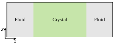
Figure 1: Sketch of the fluid-crystal coexistence in an elongated simulation box. Note that the simulation box is periodic in all directions.

Let us assume that we have already measured the bulk equation of state of the crystal phase. In other words, for any given number density $\rho^{X}$ near the melting density $\rho^{X}_{\mathrm{coex}}$, we know the pressure of the undeformed crystal $P^{\mathrm{ud}}(\rho^{X})$. We can then take a crystal of any density (near where we expect the melting density to be), and create a simulation box where it is in contact with a fluid as sketched in Fig. 1. We set the overall density $\rho^{\mathrm{global}}$ of the system such that it lies within the expected coexistence region of the system under consideration and check that a simulation at this point results in a (meta)stable two-phase coexistence can be simulated. In this geometry, the periodic boundary conditions allow deformation of the crystal in only one direction: it can elongate or compress along the $z$ direction. The $x$ and $y$ directions are fixed by the periodic boundaries, which also prevent shear deformations . If our choice of $\rho^{X}_{0}$ results in an unstrained crystal then the pressure tensor inside the crystal phase is isotropic, i.e.

$$P^{X}_{ij}=P^{\mathrm{ud}}(\rho^{X})\delta_{ij},$$ (1)

where $P^{X}_{ij}$ denotes the pressure of the crystal. In general, however, equilibration of the direct coexistence simulation will lead to a deformed crystal, where the lattice spacing along the $z$-axis is stretched by a factor $\epsilon_{zz}=\rho^{X}_{0}/\rho^{X}$, with $\rho^{X}_{0}$ and $\rho^{X}$ the initial and average values of the crystal density, respectively. The normal component of the pressure tensor $P^{\mathrm{X}}_{zz}$ inside the coexisting crystal phase can then be written as

$$P^{\mathrm{X}}_{zz}(\rho^{X}_{0},\epsilon_{zz})=P^{\mathrm{ud}}(\rho^{X}_{0})-B_{zzzz}(\rho^{X}_{0})\epsilon_{zz}+\mathcal{O}(\epsilon_{zz}^{2}),$$ (2)

where $B_{zzzz}$ is the effective elastic constant Ray (1989) of the crystal corresponding to a pure expansion along the $z$-axis. Mechanical equilibrium requires that the $P^{\mathrm{global}}_{zz}$ component of the pressure tensor is homogeneous throughout the system (see SI), and hence $P^{\mathrm{global}}_{zz}=P^{\mathrm{X}}_{zz}$. Hence, to determine the conditions where the crystal phase is undeformed ($\epsilon_{zz}=0)$ we simply have to find the choice of $\rho_{0}^{X}$ where

$$P^{\mathrm{global}}_{zz}(\rho_{0}^{X})=P^{\mathrm{ud}}(\rho_{0}^{X}).$$ (3)

In practice, this means that determining coexistence conditions requires that we find the crossing point between the functions $P^{\mathrm{global}}_{zz}(\rho_{0}^{X})$, measured in direct coexistence simulations, and $P^{\mathrm{ud}}(\rho_{0}^{X})$, measured in the bulk crystal phase.

To see how this works, we will work through this method in detail for the hard-sphere model, and then show extensions to other model systems.

II.2 Fluid-FCC crystal coexistence in hard spheres

An ideal model system for testing methods to determine phase boundaries is the hard-sphere model, as the phase behavior has been extensively studied using a variety of methods (see Ref. Royall et al., 2023 for an overview). The hard-sphere model consists of spheres of diameter $\sigma$ which are not allowed to overlap, but otherwise have no interaction. Its phase behavior consists of a fluid at densities below the freezing density $\rho_{\mathrm{coex}}^{F}\sigma^{3}\simeq 0.939$, a face-centered cubic crystal above the melting density $\rho_{\mathrm{coex}}^{X}\sigma^{3}\simeq 1.037$, and a coexistence region in between. The corresponding coexistence pressure is $\beta P\sigma^{3}\simeq 11.56$, where $\beta=1/k_{B}T$, with $k_{B}T$ the thermal energy.

We use the event-driven molecular dynamics (EDMD) simulation code from Ref. Smallenburg, 2022 to simulate both the bulk crystal phase and the direct coexistences and measure the pressure tensor. Note that for hard spheres, the $NVT$ ensemble and $NVE$ ensemble essentially coincide, since the particles do not have any energetic interactions.

We first determine the bulk equation of state $P^{\mathrm{global}}_{zz}(\rho_{0}^{X})$ in the vicinity of the melting point. Next, we construct initial configurations for a range of densities $\rho^{X}_{0}\in\{1.025,1.0275,1.030,\ldots,1.050\}$, by placing particles on an FCC lattice oriented with the square (100) face perpendicular to the interface in an elongated box chosen to be approximately three times longer in the $z$-direction than in the $x$ and $y$ directions. We then add additional empty space on one side of the crystal in the $z$-direction in order to reach an overall system density $\rho^{\mathrm{global}}=0.99$. After equilibration, the system reaches a stable fluid-crystal coexistence (see Fig. 2b for an example). During the simulation, we measure the global stress tensor $P^{\mathrm{global}}_{ij}$. In Fig. 2a, we plot both $P^{\mathrm{global}}_{zz}(\rho^{X}_{0})$ (blue line) and $P^{\mathrm{ud}}(\rho^{X}_{0})$ (red line) for a relatively small system size. The crossing point between these two lines then gives us the melting density $\rho_{\mathrm{coex}}^{X}\sigma^{3}=1.03749$ and coexistence pressure $\beta P_{\mathrm{coex}}\sigma^{3}=11.5524$ for this system size ($N\simeq 4000$ particles in the direct coexistence simulation).

Fig. 2a shows that the crossing point between $P^{\mathrm{global}}_{zz}$ and $P^{\mathrm{ud}}$ essentially coincides with a minimum in $P^{\mathrm{global}}_{zz}$. This can be understood when considering the fact that for each choice of $\rho^{X}_{0}$, the measured value of $P^{\mathrm{global}}_{zz}$ represents the pressure at which the fluid becomes metastable with respect to a crystal with this deformation. In equilibrium, the fluid will freeze as soon as there is any crystal phase more stable than the fluid. Hence, the realization of the crystal that corresponds to the lowest coexistence pressure must correspond to the true equilibrium phase transition.

In principle, this provides another avenue for estimating the coexistence pressure. However, in practice, it is much harder to accurately determine the minimum in $P^{\mathrm{global}}_{zz}$ than its crossing point with $P^{\mathrm{ud}}$. This is readily visible from Fig. 2a, as the steepness of the red line ($P^{\mathrm{ud}}$) indicates that small errors in the measurement of $P^{\mathrm{global}}_{zz}$ will not strongly affect the predicted coexistence pressure.

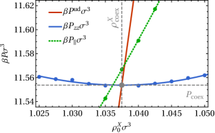
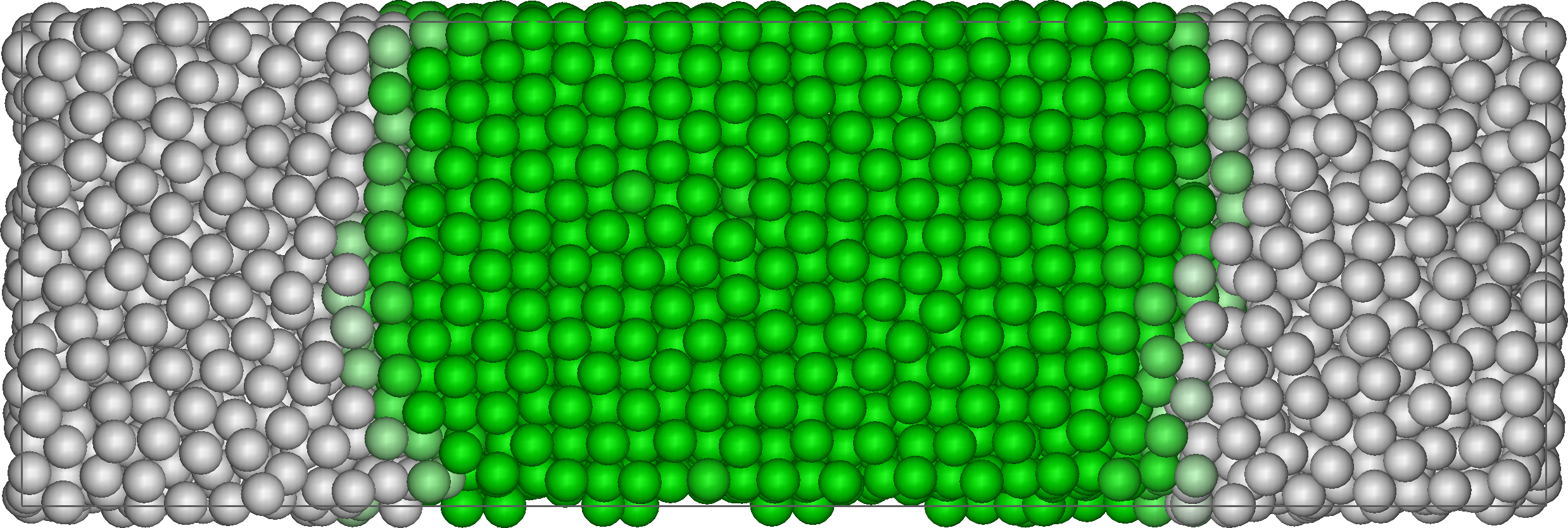
Figure 2: Direct coexistence approach for a hard-sphere system of $N=4116$ particles. The plot shows the behavior of the pressure $P^{\mathrm{global}}_{zz}$ normal to the interface as a function of the lattice spacing of the initial crystal $\rho^{X}_{0}$ (blue line). The coexistence point (gray dot) is determined as the crossing point of this line with the bulk equilibrium equation of state (red line). Note that at the point of equilibrium coexistence, the pressure component parallel to the interface ($P_{\parallel}$, green dashed line) is not the same as $P^{\mathrm{global}}_{zz}$, due to the stresses exerted by the interface. The snapshot shows a typical configuration from the direct coexistence simulation. As a guide to the eye, particles are colored based on the crystallinity of their local environment, using the averaged bond order parameter $\bar{q}_{6}$ Lechner and Dellago (2008).

a)     FCCA	FCCB	HCP

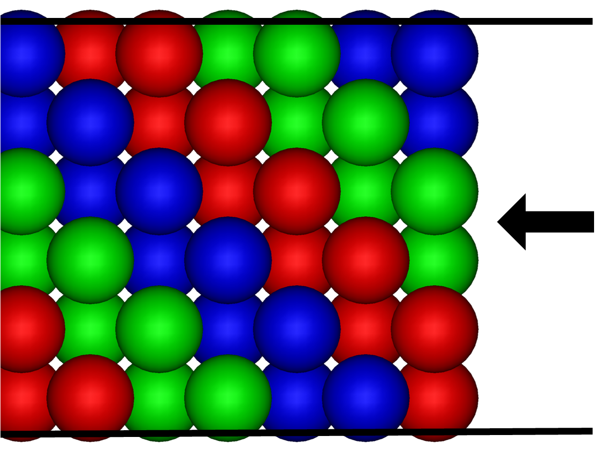
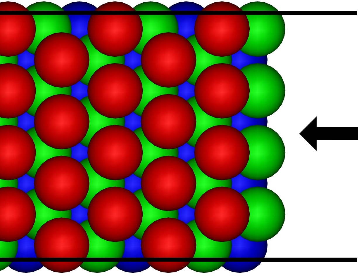
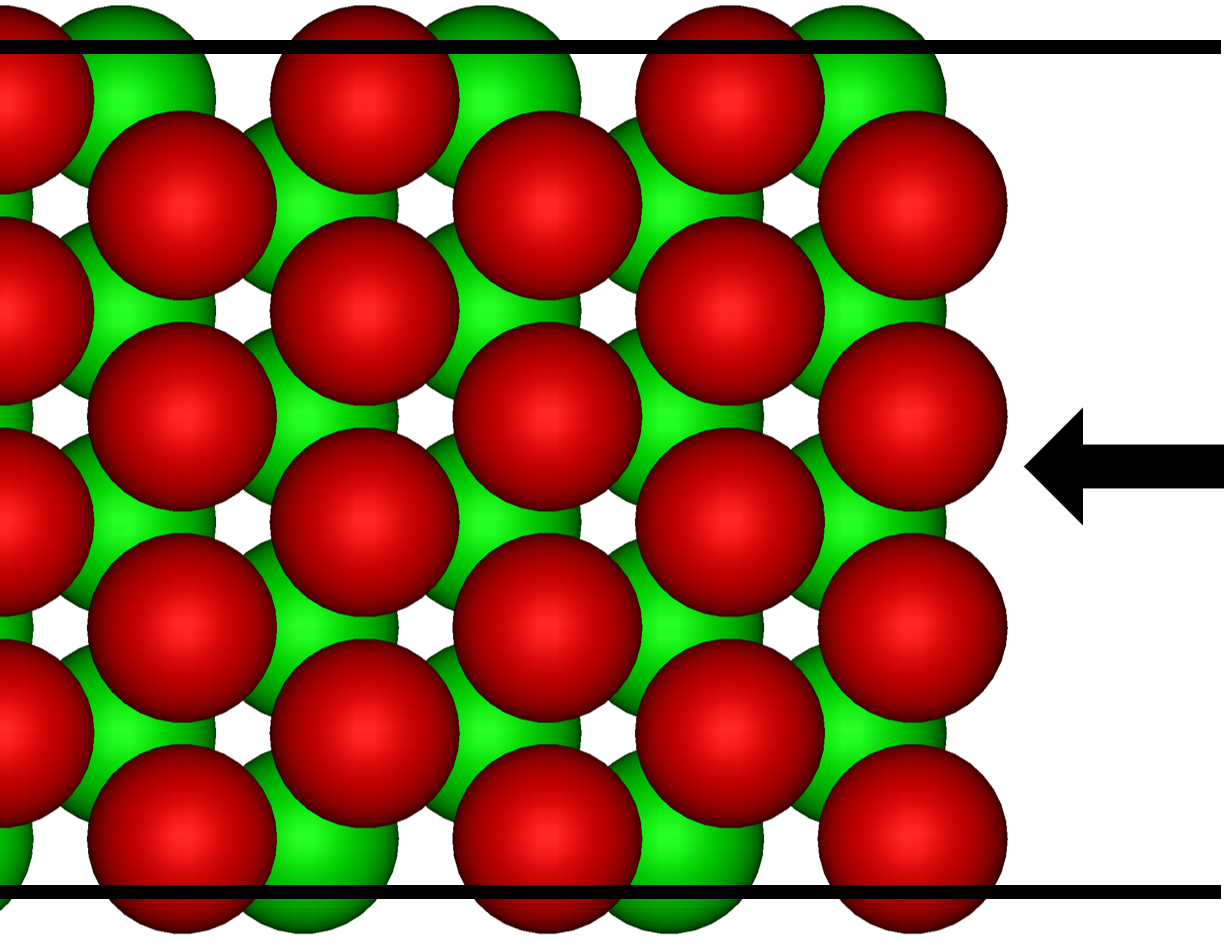
b)

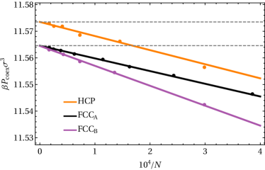
c)

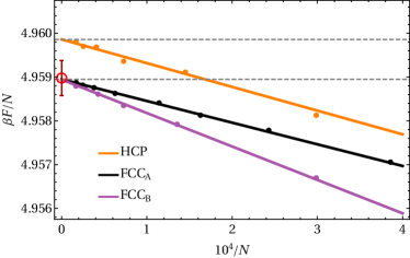
Figure 3: a) Schematic images of the crystal orientations. In each image, the arrow points at the interface facing the fluid. b) Coexistence pressure as a function of system size (characterized by the total number of particles $N$ in the direct coexistence simulations), for HCP and two different orientations of FCC. c) Helmholtz free energy of the crystal phase at density $\rho\sigma^{3}=1.0409$ (slightly above melting) as a function of system size. The red point represents the value obtained by Frenkel and Smit (2002) and its corresponding error bar. For both a) and b), the solid lines are linear fits to the data for $N\geq 5000$, and the dashed lines indicate the values obtained by extrapolating these fits to $N\to\infty$.

Also shown in Fig. 2a is the behavior of $P^{\mathrm{global}}_{\parallel}=(P^{\mathrm{global}}_{xx}+P^{\mathrm{global}}_{yy})/2$ as measured from our direct coexistence simulations. We emphasize the deviation between $P^{\mathrm{global}}_{zz}$ and $P^{\mathrm{global}}_{\parallel}$ at the point of equilibrium coexistence. This difference can be directly linked to the free-energy cost associated with ”stretching” the interface, also known as the surface stress $f$ Davidchack and Laird (1998). Although not important to the determination of the coexistence conditions, this further shows why the assumption or requirement that the global pressure is isotropic in the direct coexistence simulation is not technically correct. We note, however, that in the limit of infinite system sizes, this deviation vanishes.

The coexistence pressure and melting density obtained from Fig. 2a contain finite-size effects. To quantify these effects and obtain a prediction for the infinite-system coexistence conditions, we repeat the same calculation for system sizes ranging from $N^{\mathrm{global}}\simeq 1500$ to $6\cdot 10^{4}$ particles. We plot the resulting coexistence pressures in Fig. 3a as a function of the inverse system size (black line). Extrapolating the behavior to infinite system size, we obtain $\beta P_{\mathrm{coex}}\sigma^{3}=11.5646(5)$, which is in excellent agreement with the best known predictions in literature (see Table 1). Note that as expected, finite-size effects shift the observed coexistence pressure to lower values for smaller systems, as the periodic boundaries help stabilize the crystal phase.

Source	Method	$\rho_{\mathrm{f}}\sigma^{3}$	$\rho_{\mathrm{m}}\sigma^{3}$	$\beta P_{\mathrm{coex}}\sigma^{3}$	$N$
Davidchack and Laird (1998)	Direct coex. ($NVT$)	0.938	1.037	11.55(5)	10752
Frenkel and Smit (2002)	Free energy	0.9391	1.0376	11.567	$\infty$
Fortini and Dijkstra (2006)	Free energy	0.939(1)	1.037(1)	11.57(10)	-
Vega and Noya (2007)	Free energy	0.9387	1.0372	11.54(4)	$\infty$
Noya et al. (2008)	Direct coex. ($NP_{z}T$)	0.9375(14)	1.0369(33)	11.54(4)	5184
Zykova-Timan et al. (2010)	Direct coex. ($NP_{z}T$)	0.949	1.041	11.576(6)	$160000$
Moir et al. (2021)	Free energy	0.93890(7)	1.03715(9)	11.550(4)	$\infty$
This work	Direct coex. ($NVT$)	0.93918(1)	1.0375(3)	11.5646(5)	$\infty$

Table 1: Comparison of the predicted hard-sphere phase coexistence conditions to literature values. Note that all of these predictions neglect the effects of defects (see Discussion). In the last column, the dash(-) indicates that the treatment of system size was not reported.

In the above, we have made the choice to orient the FCC crystal with its square crystal plane facing the fluid. In principle, the coexistence conditions (in the thermodynamic limit) should be independent of the crystal orientation. To test this, we have repeated our calculation with the FCC crystal oriented such that the hexagonal planes in the crystal are aligned with the $xz$-plane of the box, as shown in Fig. 3a. As a result, the plane facing the fluid is perpendicular to these hexagonal planes. The resulting coexistence pressures are shown as the purple line in Fig. 3. As expected, for small systems the orientation matters, as the finite-size effects are different for different orientations of the crystal. However, in the limit of large systems, the two lines converge towards indistinguishable values.

II.3 Fluid-HCP coexistence in hard spheres

It is straightforward to extend our approach to crystals without cubic symmetry, for instance the hexagonal close packed (HCP) in hard spheres. For such non-cubic crystals, the lattice parameters of the stable crystal phase (i.e. the lengths and directions of the vectors spanning the unit cell) are generally dependent on the density. Hence, the determination of the equation of state should be done while taking into account the possibility of lattice deformations (e.g. in an isotension ensemble). This then also provides the shape of the crystal lattice as a function of the density. The obtained crystal lattice for each density can then be directly used in the direct coexistence simulation, by adapting the shape of the simulation box in the $xy$ plane.

To further test the sensitivity of our method, we explore the HCP-fluid coexistence in systems of hard spheres. The HCP crystal in hard spheres is known to be metastable with respect to the FCC crystal, but is extremely close in free energy. Hence, its coexistence pressure with the fluid is expected to be slightly higher than that of the FCC phase. As a first step to predicting this coexistence, we determine the pressure and lattice parameters of the HCP crystal as a function of density. Due to the hexagonal symmetry of the HCP lattice, the only parameter we have to determine is the ratio $c/a$ of the unit cell, where $a$ is lattice spacing inside the close-packed hexagonal layers and $c$ the height of the unit cell. For equilibrium hard-sphere crystals close to melting, this ratio is known to be close to the idealized value $\sqrt{8/3}$ Pronk and Frenkel (2003).

In order to continue using the same EDMD simulations in a constant-volume ensemble, we measure the lattice parameter $c/a$ by performing at each density simulations for several different values $\sqrt{8/3}-c/a\in\{0,2.5\cdot 10^{-4},...1.0\cdot 10^{-3}\}$, and identifying the deformation for which the pressure tensor is isotropic (see SI).

We then use the resulting lattice parameters as a function of density to initialize our direct coexistence simulations, where we orient the HCP crystal such that the hexagonal planes in the crystal are again aligned with the $xz$-plane of the box, as shown in Fig. 3. We plot the resulting coexistence pressures in Fig. 3 along with the FCC results. As expected, we observe that the coexistence pressure for HCP is higher than that of FCC, by approximately $0.009k_{B}T/\sigma^{3}$.

II.4 Calculating crystal free energies

Direct coexistence simulations also provide a straightforward avenue to determine the free energy of crystal phases. At coexistence, the chemical potentials of the fluid and crystal phase coincide. Hence, knowing the chemical of the fluid also implies that we know the chemical potential of the crystal. The chemical potential of the fluid can usually be straightforwardly obtained from its equation of state via thermodynamic integration (see Methods). The Helmholtz free energy of the crystal at coexistence is then given by

$$\frac{F^{X}(\rho_{\mathrm{coex}}^{X})}{N}=\mu_{\mathrm{coex}}-\frac{P_{\mathrm{coex}}}{\rho_{\mathrm{coex}}^{X}}.$$ (4)

Once this is known, we can obtain the free energy at any density inside the crystal regime via thermodynamic integration over the equation of state of the crystal Frenkel and Smit (2002):

$$\frac{\beta F^{X}(\rho)}{N}=\frac{\beta F^{X}(\rho_{\mathrm{coex}}^{X})}{N}+\int_{\rho_{\mathrm{coex}}^{X}}^{\rho}\mathrm{d}\rho^{\prime}\frac{\beta P^{\mathrm{ud}}(\rho^{\prime})}{(\rho^{\prime})^{2}}.$$ (5)

Using this approach, we calculate the free energy of the crystal at a density of $\rho\sigma^{3}=1.0409$, where we can compare to the result of Frenkel and Smit (2002) obtained using Einstein integration and finite-size scaling. We plot the results for both our FCC and HCP crystals in Fig. 3b for different system sizes, and include the extrapolated infinite-size result of Frenkel and Smit (2002) for FCC as a benchmark. Clearly, for both FCC orientations our free energies converge to the same free energy, while the HCP value is significantly higher. This allows us to calculate the free-energy difference between FCC and HCP, which we estimate to be $9.7\cdot 10^{-4}k_{B}T$ per particle at this density. This is in excellent agreement with past calculations using Einstein integration Frenkel and Ladd (1984); Bolhuis et al. (1997); Mau and Huse (1999), which estimate the difference to be approximately $0.001k_{B}T$ per particle near melting.

II.5 Yukawa particles

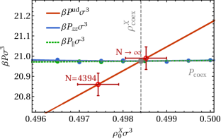
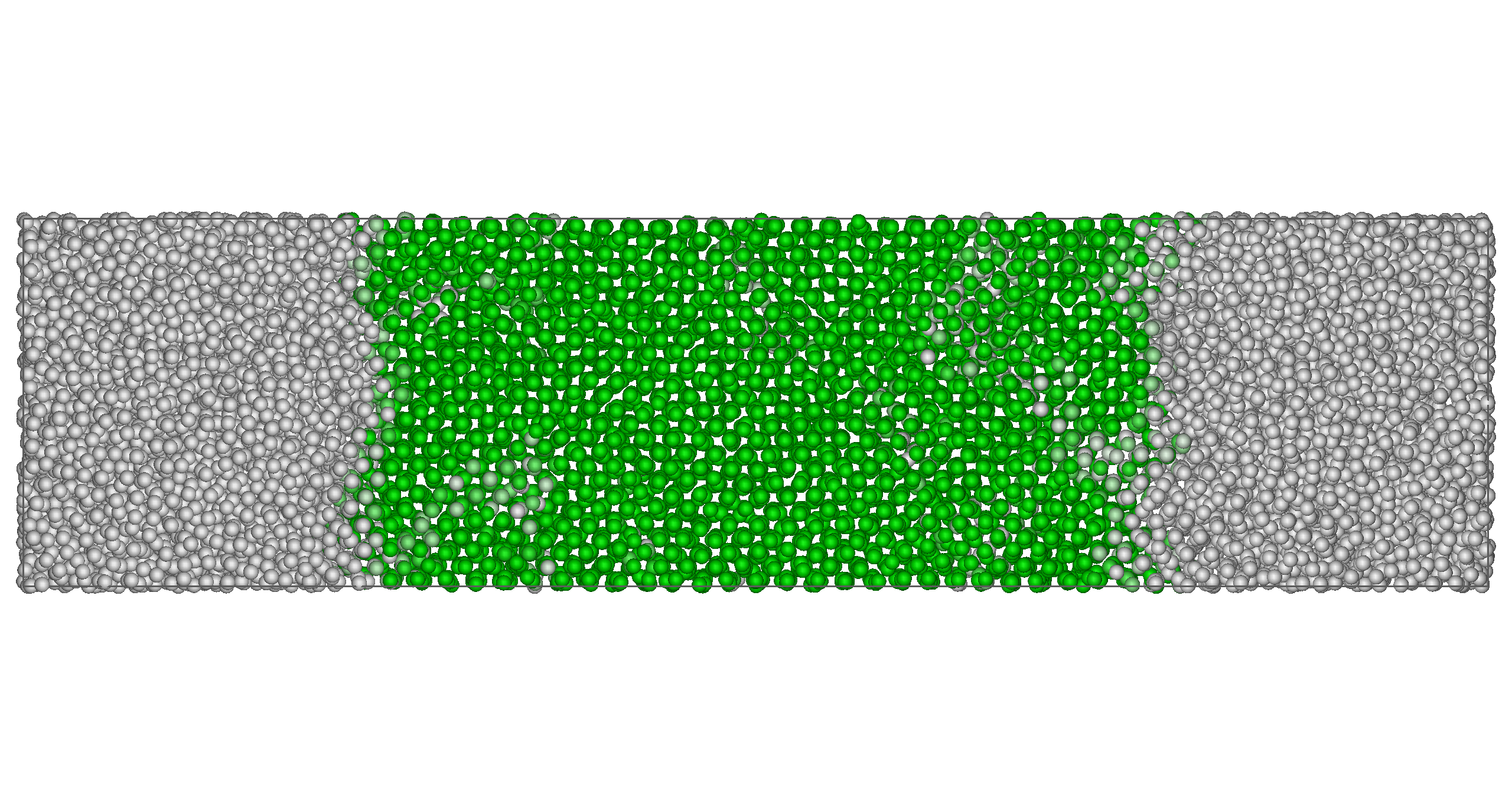
Figure 4: Direct coexistence simulation of the Yukawa model with inverse screening length $\kappa\sigma=4$, contact value $\beta\epsilon=20$, and cutoff range $r_{c}/\sigma=4.5$. The red circles indicates the predictions from free-energy calculations in the thermodynamic limit ($N\to\infty$) and for crystal system size $N=4394$. The latter corresponds to a crystal in a cubic box containing the same number of unit cells along each axis as used in the $x$ and $y$ directions of the long box simulations. As a guide to the eye, particles are colored based on the crystallinity of their local environment, using the averaged bond order parameter $\bar{q}_{6}$ Lechner and Dellago (2008).

In order to illustrate the general nature of our methodology, we now turn our attention to point particles interacting via the Yukawa (or screened Coulomb) potential, given by

$$V_{\mathrm{Yuk}}(r)=\epsilon\frac{\exp(-\kappa(r-\sigma))}{r/\sigma},$$ (6)

with $\sigma$ an effective particle size, $\epsilon$ the contact value of the potential at $r=\sigma$, and $\kappa$ the inverse screening length. In particular, we focus on a system with an inverse screening length $\kappa\sigma=4$, and a contact value $\epsilon/k_{B}T=20$, which is known to form a body-centered cubic (BCC) crystal phase upon freezing Hynninen and Dijkstra (2003). The interaction potential was truncated and shifted to zero at a cutoff distance $r_{c}=4.5\sigma$.

We note that the fluid-BCC coexistence region in this model is expected to be very narrow Hynninen and Dijkstra (2003): the predicted width of the coexistence region is less than a percent of the melting density. Fluctuations in the amount of crystal phase in the direct coexistence simulation will therefore only weakly impact the densities of the two phases, and hence their free energies. As a result, we expect (and observe) larger fluctuations in the amount of crystal in this system in comparison to the hard-sphere system, necessitating long simulations to obtain good statistical averages. Similarly, large system sizes are required in order to avoid full crystallization or melting of the system as a result of these fluctuations.

The results of the direct coexistence approach are shown in Fig. 4, where we again determine the crossing between the $P^{\mathrm{global}}_{zz}$ and $P^{\mathrm{ud}}$ as a function of the initial crystal density, for a total system size of $N=17453$ particles. The simulations were performed using the molecular dynamics simulation package LAMMPS Thompson et al. (2022), using a Nosé-Hoover thermostat to keep the temperature fixed.

To confirm our result, we also predict the phase coexistence using free-energy calculations (red circles in Fig. 4, see Methods), finding good agreement. Note that the narrow coexistence region also impacts the sensitivity of our free-energy-based predictions to statistical or systematic errors: a (reasonable) estimated error of $0.001k_{B}T$ in the crystal free energy would give rise to a shift of $\Delta P\approx 0.05k_{B}T/\sigma^{3}$ in the predicted coexistence pressure, giving rise to the large error bars in Fig. 4. This is approximately five times as large as the corresponding $\Delta P$ would be in the hard-sphere system. In other words, the narrow coexistence region makes it more cumbersome to obtain an accurate prediction for the coexistence conditions in both methodologies. Similarly, the coexistence pressure is rather sensitive to finite-size effects in the free-energy calculations. As shown in Fig. 4, the coexistence pressure shifts noticeably as we change the size of the crystal used in our free-energy calculations.

II.6 Patchy disks

Finally, to demonstrate the applicability of this method to systems of anisotropic particles, we examine a two-dimensional model consisting of hard disks decorated with equally spaced attractive patches. Depending on the number and size of the attractive patches, patchy particles in two dimensions can form a variety of (quasi)crystalline structures Doye et al. (2007); Doppelbauer et al. (2010); van der Linden et al. (2012). For simplicity, we focus on four-patch particles, modeled using the Kern-Frenkel model (see Methods for details). In this model, two particles can bond when their attractive patches align. Each bond contributes a fixed energy $\epsilon<0$ to the potential energy of the system. Since the 4 patches are evenly spaced around the perimeter of each particle at relative angles of $\pi/2$, the energetic ground state of the system trivially consists of a square lattice in which each particle is bonded to four neighbors.

We determine the fluid-crystal coexistence conditions for this model at bonding energy of $\epsilon/k_{B}T=-3.0$ using both free-energy calculations (see Methods) and the direct coexistence approach. The results are shown in Fig. 5a. The result is in close agreement with the prediction from the (significantly more cumbersome) free-energy calculations (red circle in Fig. 5a).

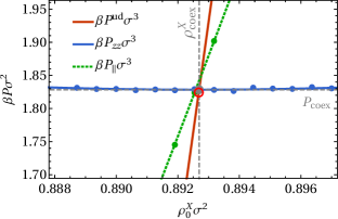
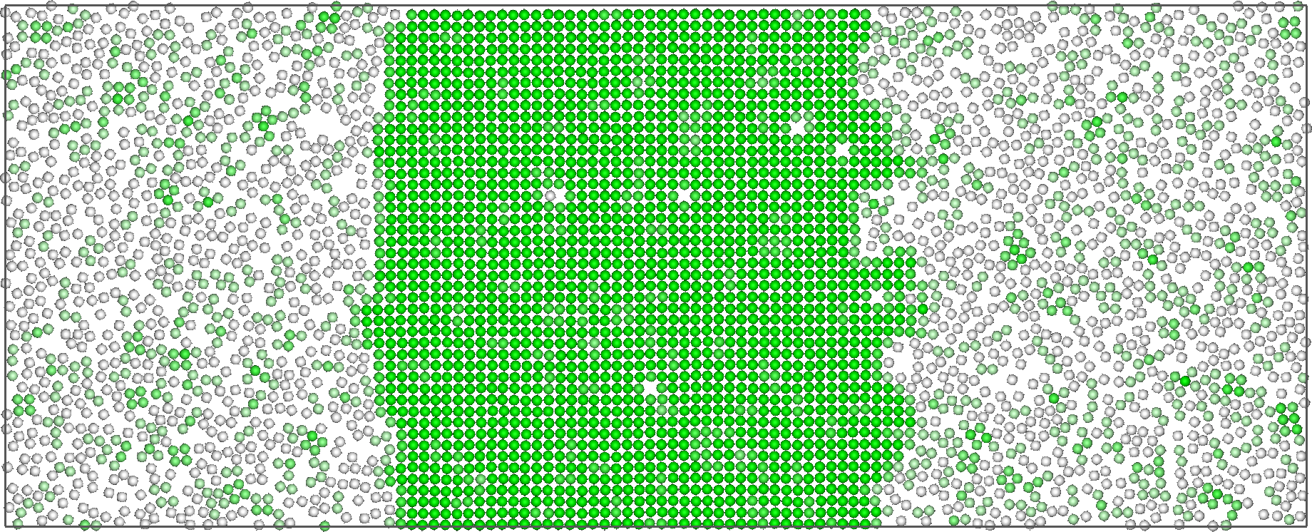
Figure 5: Direct coexistence simulation of the 4-patch Kern-Frenkel model at temperature $\epsilon/k_{B}T=-3.0$. In the plot on the left, the red circle indicates the result from free-energy calculations (statistical error bars are smaller than the point). The particles in the snapshot are colored based on the number of bonds formed by their patches.

III Discussion and Conclusions

We have presented a simple, accurate method to predict fluid-crystal coexistences based on direct coexistence simulations in the $NVT$ ensemble. As the algorithm is based on standard global pressure calculations, it can be used together with essentially any simulation method, and is hence compatible with any commonly used simulation package.

As a brief recap, to find the fluid-crystal coexistence conditions for a monodisperse system, we:

1. Determine the crystal equation of state $P^{\mathrm{ud}}(\rho^{X})$. This includes identifying the lattice parameters as a function of density.

2. Perform a series of direct coexistence simulations with different initial crystal densities $\rho^{X}_{0}$, and measure $P^{\mathrm{global}}_{zz}(\rho^{X}_{0})$.

3. Find the crossing point between $P^{\mathrm{global}}_{zz}(\rho^{X}_{0})$ and $P^{\mathrm{ud}}(\rho^{X}_{0})$. The density and pressure of the crossing point are the melting density $\rho_{\mathrm{coex}}^{X}$ and coexistence pressure $P_{\mathrm{coex}}$ respectively.

4. To obtain the freezing density, we can additionally measure the fluid equation of state $P^{F}(\rho)$, and find the density $\rho_{\mathrm{coex}}^{F}$ at which the fluid pressure equals $P_{\mathrm{coex}}$.

This method avoids the stochastic nature of the $NP_{z}T$ approach of e.g. Refs. Noya et al. (2008); Espinosa et al. (2013), and therefore the need to run multiple simulations at the same state point to determine a melting probability. It is also significantly simpler than the interface pinning method Pedersen et al. (2013), which requires the introduction of a biasing potential and an order parameter to track the overall crystallinity of the system. Finally, in comparison to the approach of Davidchack and Laird Davidchack and Laird (1998), our method avoids the need to measure local stress profiles and manual adjustments of the simulation box to these measurements.

In comparison to free-energy calculations using e.g. the Frenkel-Ladd method Frenkel and Ladd (1984), the direct-coexistence approach we propose here is much easier to implement. Most importantly, the direct coexistence approach allows for the determination of the coexistence densities and pressures without requiring a numerical integration over a series of simulation results. As such integrations can easily introduce numerical errors (due to a finite integration step size, the need to carefully choose integration limits, etc.) this immediately makes the direct coexistence approach significantly less error-prone. Additionally, free-energy calculations can present a number of pitfalls that can introduce errors in the result, which may be difficult to detect. For instance, in the Yukawa model studied here, simulations of the crystal close to melting allow for the spontaneous diffusion of particles within the lattice. If this occurs in the simulations associated with the Frenkel-Ladd integration (typically at low spring constants), special care must be taken to avoid a systematic error in the resulting free energy. Free-energy calculations also must explicitly take into account any configurational entropy associated with the crystal phase, as may occur in e.g. ice Berg et al. (2007), crystals of dumbbell-shaped particles Marechal and Dijkstra (2008), or quasicrystals Fayen et al. (2024). In contrast, this configurational entropy is inherently taken into account by the direct coexistence approach.

It is important to note that the direct coexistence method also comes with a few caveats. First, defects are not accurately taken into account in the methodology described above. In the direct coexistence simulations, point defects such as vacancies and interstitials are free to diffuse into and out of the crystal phase (as is visible in Fig. 5), and hence for sufficiently long simulation times we would expect these simulations to correctly incorporate them. However, this may require long simulation times in practice. Moreover, we neglected the effects of defects on the bulk equation of state. In principle, this could be addressed with some additional effort, e.g. by measuring the defect concentration in the direct coexistence simulation (assuming it is large enough to be measurable), and checking the effect of these defects on the equation of state. We note, however, that taking into account defects in free-energy calculations also requires significant additional effort Pronk and Frenkel (2001); De Jager et al. (2021); van Der Meer et al. (2020) and is rarely done.

Secondly, it should be noted that the direct coexistence approach is generally more computationally expensive than free-energy calculations. Equilibrating the explicit interface between the two coexisting phases and sampling its fluctuations over time requires simulations over longer time scales than sampling the behavior of the single-phase simulations required for a prediction of phase coexistence based on free energies. Moreover, the system sizes required to maintain a stable coexistence are significantly larger than those required to simulate a pure fluid or crystal in a reasonable approximation of the the thermodynamic limit. This downside is partially addressed by the simplicity of the method, which means that the simulations can be performed by existing simulation codes that have already been well-optimized or adapted for parallel or GPU computing. However, if the model of interest has interactions that are computationally expensive, or requires very large system sizes to realize a stable interface, the computational cost may become prohibitive.

Finally, we point out that direct coexistence methods are not suitable for solid-solid transitions, as two unstrained crystals can typically not occupy the same simulation box Frenkel and Smit (2002). Nonetheless, in some cases, such as the case of hard-sphere HCP presented here, direct coexistence can still be useful if a metastable fluid-crystal coexistence can be simulated. The resulting crystal free energy at melting can then be used as a reference point for thermodynamic integration to other state points. However, for crystal phases that cannot form a metastable coexistence with a fluid, other methods would be required.

Despite these caveats, the $NVT$ direct coexistence method presented here is a highly accurate and convenient method for the prediction of fluid-crystal phase coexistences. As shown by our hard-sphere example, it is at least as accurate as free-energy calculations. Moreover, as we show with the Yukawa and patchy systems, the method is directly applicable to any fluid-crystal phase boundary. In short, $NVT$ direct coexistence is a powerful method that we expect to become a staple technique for the determination of crystal phase boundaries.

IV Methods

IV.1 Hard spheres

We simulate systems of $N$ hard spheres of identical mass $m$ and diameter $\sigma$ in a volume $V$, using a the EDMD simulation code of Ref. Smallenburg, 2022, adapted to measure the pressure tensor. We do not make use of a thermostat, and hence the total energy of the system (which consists only of the kinetic energy) is fixed. This in turn also fixes the temperature $T$. During the simulation, we measure the pressure tensor $P_{ij}$ by keeping track of the momentum transfer during each collision:

$$P_{ij}=\rho k_{B}T\delta_{ij}-\frac{1}{V}\frac{\sum_{k}m\,\delta v_{i}^{(k)}\,\delta r_{j}^{(k)}}{t_{\mathrm{end}}-t_{\mathrm{start}}},$$ (7)

where $\delta_{ij}$ is the Kronecker delta, $\rho=N/V$ the number density, and $k_{B}$ Boltzmann’s constant. The sum runs over all collisions $k$ occurring between times $t_{\mathrm{start}}$ and $t_{\mathrm{end}}$. For each collision, $\delta\mathbf{r}^{(k)}$ and $\delta\mathbf{v}^{(k)}$ denote the relative position and velocity of the two particles involved in the collision, respectively.

To determine the equation of state, we simulate bulk crystals for a range of different system sizes and in different orientations in order to make the size of the system similar to that of the direct coexistence simulation. However, in practice the finite size effects on the equation of state have a negligible effect on the overall determination of the coexistence conditions: repeating our calculations with the $Z_{S2}$ hard-sphere crystal equation of state by Pieprzyk et al. (2019) yields essentially indistinguishable results, especially for larger system sizes.

For the direct coexistence simulations, we use system sizes ranging from $N\simeq 1500$ particles to $N\simeq 60\,000$ particles, depending on the chosen crystal orientation. The simulations were typically run for simulation times of at least $10^{5}\tau$, where $\tau=\sqrt{\beta m\sigma^{2}}$ is the time unit of our simulation. This is typically enough to obtain a good estimate of the coexistence conditions, especially for larger system sizes. However, some simulations were run for up to 10 times longer to decrease noise.

After obtaining the coexistence pressure, we determine the freezing density $\rho_{\mathrm{coex}}^{F}$ using the mKLM hard-sphere fluid equation of state of Ref. Pieprzyk et al. (2019). Using the same equation of state, we calculate the chemical potential via thermodynamic integration from an ideal gas:

$$\mu_{\mathrm{coex}} = \frac{F^{F}_{\mathrm{coex}}}{N}+\frac{P_{\mathrm{coex}}}{\rho_{\mathrm{coex}}^{F}}$$ (8)

$$\frac{\beta F^{F}_{\mathrm{coex}}}{N} = \log(\rho_{\mathrm{coex}}^{F}\Lambda^{3})-1+\int_{0}^{\rho_{\mathrm{coex}}^{F}}\mathrm{d}\rho^{\prime}\frac{\beta P(\rho^{\prime})-\rho^{\prime}}{(\rho^{\prime})^{2}},$$

with $\Lambda^{3}$ the thermal wavelength which we set equal to $\sigma$. Note that the value of $\Lambda$ does not affect the phase behavior, as it only results in a constant shift of the free energy in all phases. Hence, we choose to set it equal to $\sigma$ as is commonly done in free-energy calculations of hard spheres.

IV.2 Yukawa particles

We perform the direct coexistence simulations for the Yukawa system using the LAMMPS simulation packageThompson et al. (2022); Brown et al. (2011). An example script is provided in the SI. The system consists of $N=17453$ atoms placed within a simulation box whose $z$-axis was approximately four times longer than the $x$ and $y$ axes, at total density $\rho^{\mathrm{global}}\sigma^{3}=0.4962$, for which the system is approximately evenly distributed among the two phases. Note that due to the large fluctuations in crystal size occurring in these simulations, smaller system sizes often resulted in complete melting or freezing of the system. In the initial configuration, half of the particles are placed on a BCC lattice with the $(100)$ crystallographic direction lying along the $z$-axis and 13 unit cells along the short sides. The other half are placed randomly in the remaining volume of the box. We perform a short energy minimization before the start of the run to reduce the initial forces between particles in the starting configuration. Additional configurations at different values of $\rho_{0}^{X}$ are then generated by rescaling of the simulation box. We carry out the $NVT$ simulations for a time of $2.5\cdot 10^{6}\tau$ with an integration time step $dt=5\cdot 10^{-3}\tau$. As a thermostat, we use Nosé-Hoover chains with 30 oscillators in the chain and a damping parameter $\tau_{d}=2.0\tau$. However, other reasonable choices of thermostatting parameters (e.g. changes in damping parameter or using only a simple Nosé-Hoover thermostat without chaining) do not noticeably affect our results.

In order to verify the coexistence values obtained from the direct coexistence simulations in the Yukawa system, we additionally determine the coexistence conditions via a free-energy route.

We determine the equation of state of the bulk fluid and crystal phases using Monte Carlo (MC) simulations in the $NVT$ ensemble. These simulations are all initialized as a perfect BCC crystal of 2000 particles. Additionally, we use MC simulations in the $NPT$ ensemble of a fluid of 2000 particles to determine the equation of state of the metastable fluid.

To determine the free energy of the fluid phase, we use thermodynamic integration of the equation of state to obtain the free energies as a function of density, using the ideal gas as a reference system Frenkel and Smit (2002):

$$\frac{\beta F}{N}=\log(\rho\Lambda^{3})-1+\int_{0}^{\rho}\frac{\beta P(\rho^{\prime})-\rho^{\prime}}{{\rho^{\prime}}^{2}}\mathrm{d}\rho^{\prime}.$$ (9)

Here, $\Lambda$ is the thermal De Broglie wavelength, which we again set equal to $\sigma$. To perform the integral, we fit the equation of state of the fluid using the virial expansion up to 10th order, for which we calculated $B_{2}$ analytically.

For the crystal, we again use thermodynamic integration (analogous to Eq. 5), using a 6th order polynomial fit to the equation of state and starting from a reference free energy at effective packing fraction $\eta=\pi\rho\sigma^{3}/6=0.29$. We obtain this reference free energy using Einstein integration Frenkel and Ladd (1984) and correct for finite-size effects by considering systems of 686, 1024, 1458, 2000, 2662, 3456, and 4394 particles Polson et al. (2000). In this approach, the absolute free energy of the crystal is determined as a thermodynamic integration between a reference system and the crystal of interest. The reference system consists of an Einstein crystal of non-interacting particles, which are tied to their lattice sites via harmonic springs with a spring constant $\alpha$. To this end, we perform a series of MC simulations with an effective Hamiltonian given by

$$H(\lambda)=(1-\lambda)U_{\mathrm{Yuk}}(\mathbf{r}^{N})+\lambda U_{\mathrm{Ein}}^{r}(\mathbf{r}^{N}),$$ (10)

where $\lambda$ is a parameter that tunes between the Yukawa crystal ($\lambda=0$) and the Einstein crystal ($\lambda=1$), and $U_{\mathrm{Yuk}}$ is the total interaction energy of the system resulting from the Yukawa pair interactions. $U_{\mathrm{Ein}}^{r}$ is the energy resulting from the springs binding the particles to their lattice sites, given by

$$U^{r}_{\text{Ein}}=\frac{\alpha}{\sigma^{2}}\sum_{i}(\mathbf{r}_{i}-\mathbf{R}^{(i)}_{0})^{2},$$ (11)

where $\mathbf{R}^{(i)}_{0}$ are the equilibrium positions in the ideal lattice. During the simulations, the center of mass is kept fixed Frenkel and Smit (2002).

The free energy of the interacting Yukawa crystal is then determined as Frenkel and Smit (2002)

$$\frac{\beta F}{N}=3\log\frac{\Lambda}{d_{\alpha}}+\frac{1}{N}\log\frac{\rho d_{\alpha}^{3}}{N^{3/2}}-\beta\int_{0}^{1}\mathrm{d}{\lambda}\left\langle\frac{\partial H}{\partial\lambda}\right\rangle_{\lambda},$$ (12)

with $d_{\alpha}=\sqrt{\pi\sigma^{2}/\beta\alpha}$ the typical displacement of a particle in the Einstein crystal. Here, the first term represents the free energy of the Einstein crystal, the second term incorporates corrections due to the fixing of the center of mass Frenkel and Smit (2002), and the integral term represents the free-energy difference between the Einstein and Yukawa crystals (with fixed centers of mass). The subscript $\lambda$ in the integrand indicates that the measurement of $\frac{\partial H}{\partial\lambda}$ is done in a simulation where the parameter in Eq. 10 is set to $\lambda$.

We use a spring constant of $\beta\alpha=34$ for the Einstein crystal, and, for each system size, perform the numerical integration using a 10-point Gauss-Legendre quadrature Frenkel and Smit (2002) and estimate the error using an additional 11 points from the Gauss-Kronrod rule.

Using the fluid and crystal free energies, we finally find the equilibrium coexistence point by determining the conditions where the two phases have equal pressures and chemical potentials via a common-tangent construction.

IV.3 Patchy disks

We simulate systems of two-dimensional identical patchy particles of diameter $\sigma$. They interact through the Kern-Frenkel potential Kern and Frenkel (2003), involving a hard core repulsion and 4 directional attractive patches, whose angular position is evenly spaced. Specifically, the interaction potential is given by:

$$V_{KF}(\mathbf{r}_{ij},\theta_{i},\theta_{j})=V^{\textsc{HS}}(r_{ij})+V^{\textsc{SW}}({r}_{ij})f(\mathbf{r}_{ij},\theta_{i},\theta_{j})),$$ (13)

where $r_{ij}=|\mathbf{r}_{ij}|$ is the center-to-center distance between particles $i$ and $j$, and $\theta_{i}$ denotes the orientation of particle $i$. Additionally, $V^{\textsc{HS}}$ is the hard-disk potential with diameter $\sigma$, and $V^{\textsc{SW}}$ is a square-well potential, given by

$$V^{\textsc{SW}}(r)=\begin{cases}\epsilon&r\leq\lambda_{p}\\ 0&r>\lambda_{p},\end{cases}$$ (14)

where we choose the interaction range $\lambda_{p}=1.12\sigma$ and attractive strength $\epsilon=-3k_{B}T$. Finally, $f(\mathbf{r}_{ij},\theta_{i},\theta_{j})$ specifies the directionality of the interactions:

$$f(\mathbf{r}_{ij},\theta_{i},\theta_{j})=\begin{cases}1&\begin{cases}\hat{\mathbf{n}}_{\alpha}^{(i)}\cdot\hat{\mathbf{r}}_{ij}>\cos\theta\text{\,\,and}\\ \hat{\mathbf{n}}_{\beta}^{(j)}\cdot\hat{\mathbf{r}}_{ji}>\cos\theta,\\ \text{for any two patches $\alpha$ and $\beta$}\end{cases}\\ 0\end{cases}$$ (15)

where $\hat{\mathbf{n}}_{\alpha}^{(i)}$ is a unit vector in the direction of patch $\alpha$ on particle $i$, and $\hat{\mathbf{r}}_{ij}=\mathbf{r}_{ij}/r_{ij}$. The angle $\theta=7\degree$ controls the size of the patches.

The direct coexistence simulations were performed using EDMD simulations Hernández de la Peña et al. (2007); Smallenburg and Sciortino (2013), where we again measure the pressure tensor (Eq. 7). During these simulations, the temperature is kept fixed via an Andersen thermostat Frenkel and Smit (2002). In particular, we simulate systems of $N=4232$ particles, at global densities $\rho^{\text{global}}\sigma^{2}\simeq 0.714$ (at which the system is roughly evenly split into the two phases), in a simulation box whose $z$-axis is approximately 2.5 times longer than the $x$-axis, for a simulation time $10^{6}\tau$. Measurements of the pressure tensor, and relative statistical errors, were obtained over 10 independent runs per point.

We also calculate the coexistence conditions using a free-energy route. For the equation of state of the fluid we perform EDMD simulations of $N=2116$ particles for a time of $2\cdot 10^{5}\tau$ after equilibrating the system for $2\cdot 10^{4}\tau$. At low densities we perform longer simulations, to ensure sufficient statistics. Pressure values at each state point are averaged over 10 independent runs, and statistical error is also estimated. The fluid free energy is again calculated using Eq. 9, using a weighted fit on the integrand function using a 19-th order polynomial on 75 points, constraining the constant term to the analytically known second virial coefficient

$$B_{2}=\pi\sigma^{2}/2\left\{1-\left(\exp{\beta\epsilon}-1\right)n_{\text{p}}^{2}\frac{\delta^{2}}{\pi^{2}}\left[\left(\frac{\lambda_{\text{p}}}{\sigma}\right)^{2}-1\right]\right\},$$ (16)

adapted from Ref. Dorsaz et al., 2012 to the case of two-dimensional particles.

For the square crystal phase we calculate the free energy at packing fractions $\eta=0.70,0.72,0.73$ with the Frenkel-Ladd method, using Monte Carlo simulations. For these anisotropic particles, in the Einstein crystal both the position and the orientation of each particles are tied to a reference point. In addition to the positional springs of Eq. 11, we now additionally include a constraining potential for the orientations:

$$U^{\theta}_{\text{Ein}} = \sum_{i}\alpha\sin^{2}\left(\frac{n_{\text{p}}(\theta_{i}-\theta^{(i)}_{0})}{2}\right)$$ (17)

where $\theta_{i}$ is the orientation of particle $i$, and $\theta^{(i)}_{0}$ is its current orientation in the ideal lattice. We then perform a series of simulations with $\alpha$ varying from $0$ to $\alpha_{\mathrm{max}}=10^{4}$ and measure the mean values of both of the above expressions during each simulation, in a system interacting through the total potential $U_{\text{KF}}+U^{r}_{\text{Ein}}+U^{\theta}_{\text{Ein}}$. The free energy of the patchy square crystal (with $n_{p}=4$) is then given by:

$$\frac{\beta F}{N} = \log\frac{(\beta\alpha_{\mathrm{max}})^{3/2}\Lambda^{2}}{\sigma^{2}\sqrt{\pi}}+\frac{1}{N}\log\frac{\pi\rho\sigma^{2}}{N\beta\alpha_{\mathrm{max}}}$$ (18)

$$+ 2\beta\epsilon-\beta\int_{0}^{\alpha_{\text{max}}}d\alpha\left\langle\frac{U^{r}_{\text{Ein}}+U^{\theta}_{\text{Ein}}}{\alpha}\right\rangle_{\alpha},$$

where we have assumed that $\alpha_{\mathrm{max}}$ is large enough to ensure that when $\alpha=\alpha_{\mathrm{max}}$ all particles remain bonded to their four neighbors throughout the simulation, and the deviations of particles from their lattice sites are small enough that $V^{\theta}_{\mathrm{Ein}}$ is effectively harmonic.

We perform the integration from the Einstein crystal by using a 50-point Gauss-Legendre quadrature, estimating and propagating the statistical error over 10 independent runs per each point. We performed Monte Carlo (MC) NVT simulations of $N=2116$ particles for $10^{6}$ cycles, with a constrained center of mass. Finally, analogously to the Yukawa system, we obtain the free energy as a function of the density by integrating along the equation of state (Eq. 5), starting from the point at $\eta=0.70$. We then obtain the coexistence conditions via a common tangent construction, using both the fluid and crystal free energies. The error is estimated by considering the statistical error on the free energies and the numerical error on its derivative.

We did not perform finite-size analysis for the patchy system.

Data availability statement

The authors declare that the data supporting the findings of this study are available within the article and supplemental material, as well as a data package which will be published on Zenodo.

Author contributions

F.S. and L.F. designed and supervised the project. F.S. performed the hard-sphere simulations and supplied the EDMD simulation codes. G.D.M. performed the patchy and Yukawa direct coexistence simulations and the patchy free-energy calculations. M.d.J. performed the Yukawa free-energy calculations. All authors contributed to the manuscript.

References

- Frenkel and Smit (2002) D. Frenkel and B. Smit, Understanding Molecular Simulation: From Algorithms to Applications, 3rd ed., Computational Science Series No. 1 (Academic Press, San Diego, 2002).
- Chew and Reinhardt (2023) P. Y. Chew and A. Reinhardt, J. Chem. Phys. 158, 030902 (2023).
- Bruce et al. (2000) A. Bruce, A. Jackson, G. Ackland, and N. Wilding, Phys. Rev. E 61, 906 (2000).
- Wilding and Bruce (2000) N. Wilding and A. Bruce, Phys. Rev. Lett. 85, 5138 (2000).
- Chen et al. (2001) B. Chen, J. I. Siepmann, and M. L. Klein, J. Phys. Chem. B 105, 9840 (2001).
- Frenkel and Ladd (1984) D. Frenkel and A. J. Ladd, J. Chem. Phys. 81, 3188 (1984).
- Vega et al. (2008) C. Vega, E. Sanz, J. Abascal, and E. Noya, J. Phys. Condens. Matter 20, 153101 (2008).
- Bolhuis and Frenkel (1997) P. Bolhuis and D. Frenkel, J. Chem. Phys. 106, 666 (1997).
- Schilling and Schmid (2009) T. Schilling and F. Schmid, J. Chem. Phys. 131, 231102 (2009).
- Polson et al. (2000) J. M. Polson, E. Trizac, S. Pronk, and D. Frenkel, J. Chem. Phys. 112, 5339 (2000).
- Vega and Noya (2007) C. Vega and E. G. Noya, J. Chem. Phys. 127, 154113 (2007).
- Dijkstra (2013) M. Dijkstra, “Physics of complex colloids,” in Proceedings of the International School of Physics Enrico Fermi, Vol. 184 (IOS Press, 2013) p. 229.
- Moir et al. (2021) C. Moir, L. Lue, and M. N. Bannerman, J. Chem. Phys. 155, 064504 (2021).
- Opitz (1974) A. Opitz, Phys. Lett. A 47, 439 (1974).
- Ladd and Woodcock (1977) A. Ladd and L. Woodcock, Chem. Phys. Lett. 51, 155 (1977).
- Ladd and Woodcock (1978) A. Ladd and L. Woodcock, Mol. Phys. 36, 611 (1978).
- Cape and Woodcock (1978) J. N. Cape and L. V. Woodcock, Chem. Phys. Lett. 59, 271 (1978).
- Morris and Song (2002) J. R. Morris and X. Song, J. Chem. Phys. 116, 9352 (2002).
- Morris et al. (1994) J. R. Morris, C. Wang, K. Ho, and C. T. Chan, Phys. Rev. B 49, 3109 (1994).
- Yoo et al. (2004) S. Yoo, X. C. Zeng, and J. R. Morris, J. Chem. Phys. 120, 1654 (2004).
- Lanning et al. (2004) O. J. Lanning, S. Shellswell, and P. A. Madden*, Mol. Phys. 102, 839 (2004).
- Wang et al. (2005) J. Wang, S. Yoo, J. Bai, J. R. Morris, and X. C. Zeng, J. Chem. Phys. 123, 036101 (2005).
- García Fernández et al. (2006) R. García Fernández, J. L. Abascal, and C. Vega, J. Chem. Phys. 124, 144506 (2006).