Abstract

In this study, the parameter space of the Lepton Specific Two Higgs Doublet Model (LS-2HDM) is investigated to align the W-boson mass reported by the CDF experiment with recent theoretical and experimental findings. The Lepton Specific Two Higgs Doublet Model, a distinguished category within Two Higgs Doublet Models, contains two CP-even, one CP-odd, and two charged scalar bosons, which play crucial role in estimating W boson mass. First, constraints from diverse experimental data, including ATLAS 13 TeV analyses, rare B-meson decays, and Lepton Flavor Universality in tau-lepton and Z-boson decays, are determined and imposed on the parameter space of the model. These constraints are subsequently applied to potential solutions generated through random scans using SARAH 4.13.0 and analyzed using SPheno 4.0.3. The analysis indicates the possibility of realizing the CDF-reported W-boson mass up to $1\sigma$ within the low $\tan\beta$ regime ($2.5\lesssim\tan\beta\lesssim 8.0$). Furthermore, it establishes mass limits for the additional scalar boson as $164\lesssim m_{h_{2}}\lesssim 195$ GeV, $330\lesssim m_{A}\lesssim 575$ GeV, and $345\lesssim m_{H^{\pm}}\lesssim 685$ GeV. Moreover, it is observed that instead of the masses, mass differences of the new scalars of the model are more constrained to assure the CDF reported value of the W boson. Finally, all potential solutions estimating the W-boson mass within a $1\sigma$ vicinity are rigorously tested using the HiggsTools package. Remarkably, only one solution remains valid, estimating $M_{W}=80.4103$ GeV within a $2.44\sigma$ vicinity of the CDF-reported value.

I Introduction

The Standard Model (SM) has withstood rigorous testing, successfully been explaining various phenomena in particle physics. However, recent measurements of the W-boson mass at the Collider Detector at Fermilab (CDF) have revealed substantial discrepancies between experimental observations and theoretical predictions within the SM framework. The CDF reported a precise measurement of the W-boson mass using the $8.8fb^{-1}$ dataset from $p\bar{p}$ collisions with a center-of-mass energy of 1.96 TeV as [1]

$$M_{W}^{\rm CDF}=80.4335\pm 0.0094\ \text{GeV},$$ (1)

which deviates from the SM prediction $M_{W}^{\rm SM}=80.357\pm 0.006{\rm GeV}$ by $7\sigma$ [2, 3, 4, 5, 6, 7, 8, 9, 10, 11, 12, 13]. Such a notable discrepancy suggests the potential existence of new physics phenomena, necessitating a comprehensive exploration of physics Beyond the Standard Model (BSM). The inclusion of BSM particles might induce quantum corrections accountable for the deviation observed in the W-boson mass, hence they have sparked a growing interest in exploring new physics BSM, mostly by altering the oblique parameters, $S$, $T$, and $U$. These approaches include a broad range of theoretical frameworks, including effective field theory methods [14, 15, 16, 17, 18, 19, 20], supersymmetric (SUSY) models [21, 22, 23, 24, 25, 26, 27] , leptoquark models [28, 29, 30], gravitational approaches [31, 32], Little Higgs models [33], and extensions of the SM involving additional scalar singlets [34, 35, 36, 37] or triplets [38, 39, 40] . Additionally, models featuring vector-like leptons have been explored [41, 42, 43, 44, 45, 46], alongside investigations from the point of view of neutrino masses and seesaw mechanisms [47, 48], and other therotical approaches [49, 50, 51, 52, 53, 54, 55, 56, 57, 58]. Furthermore, Two Higgs Doublet Models (2HDM) have been attracting a considerable interest by providing a simple extension of SM [59, 60, 61, 62, 63, 64, 65, 66, 67, 68, 69, 70, 71, 72, 73, 74, 75, 76, 77, 78], while the Higgs bosons in its spectrum can interfere with the SM particle they can yield some deviations in W-boson mass, Lepton Flavor Universality (LFU) [79, 80, 81] , muon g-2 [82, 83, 84] through their radiative contributions. Among these efforts, certain studies specifically target the W boson mass discrepancy while also addressing the dark matter problem by choosing a focused approach on both issues within their framework [59, 33, 34, 41, 44, 58, 52, 54]. It appears that this anomaly attracts a lot of attention from several theoretical approaches, among which 2HDMs is an important one. However, while 2HDMs are widely used in understanding the W boson mass anomaly, their parameter space is limited by experimental data from several experiments [79, 80, 85, 80, 81, 86, 87, 88, 89, 90, 91]. Therefore, in this study, motivated by these theoretical and experimental efforts within 2HDM frameworks, an exploratory investigation aimed at reconciling the W boson mass discrepancy by scanning possible solutions within the 2HDM parameter space.

This study focuses on investigating the impact of the parameter space of 2HDM on the W-boson mass. Two crucial considerations are taken into account in our analyses: theoretical limitations and compatibility with the current experimental data. Theoretical limitations arise from constraints related to stability of the scalar potential and perturbativity. The predictions of 2HDMs must also align with the outcomes of various experiments, such as those involving rare decays of B-meson, Z-boson decay, tau-lepton decay, and observations from the Large Hadron Collider (LHC). To explore the implications of different types of 2HDMs within these theoretical and experimental limitations, the HiggsTools framework was utilized [92]. Among several types of 2HDMs, the Lepton Specific 2HDM (LS-2HDM) has emerged as the most promising model, providing numerous solutions that meet the experimental constraints for additional Higgs bosons. This model also enables to avoid from the current strong limits determined by recent CMS findings on scalar masses of the 2HDM, where a Generalized 2HDM was chosen [91]. The following steps are followed in this work. Firstly, the mass spectra of the scalar sector consistent with both theoretical and experimental constraints are obtained. After identifying these solutions, an analysis of the implications for Lepton Flavor Universality is conducted, particularly by taking into account the processes involving the tau-lepton and Z-boson. These analyses further constrain the parameter space of the LS-2HDM. Subsequently, the compatibility of the LS-2HDM with the observed W-boson mass by CDF is considered together with of theoretical and experimental restrictions. Finally, it is obtained that the CDF reported W-boson mass can be successfully accommodated within the framework of the LS-2HDM, and the remaining parameter space of the model is also determined.

This work is structured as follows: The second section summarizes LS-2HDM, focusing on its Higgs sector and Yukawa interactions. The third section outlines the theoretical and experimental constraints used in this analysis, along with a detailed discussion of their impacts on the parameter space. In the fourth section, the parameter space of the LS-2HDM is systematically explored, and potential solutions are provided. Finally, the last section offers discussions and concluding remarks.

II Lepton Specific 2HDM

2HDMs are obtained by extending the scalar sector of the SM with the addition of a second scalar doublet possessing the same quantum numbers as the SM Higgs Doublet. The gauge group of the 2HDMs is identical to that of the SM. In 2HDMs, eight scalar fields are introduced and following a spontaneous symmetry breaking process akin to that of the SM, three of these fields confer masses of the gauge bosons, while the remaining five fields undergo mixing, resulting in five distinct physical scalar bosons. These additional degrees of freedom present in the 2HDM have far-reaching implications for Higgs boson phenomenology. The scalar doublets of 2HDMs are given as

$$\Phi_{1}=\left(\begin{array}[]{c}\phi_{1}+i\phi_{2}\\ \phi_{3}+i\phi_{4}\end{array}\right)\qquad\text{and}\qquad\Phi_{2}=\left(\begin{array}[]{c}\phi_{5}+i\phi_{6}\\ \phi_{7}+i\phi_{8}\end{array}\right),$$ (2)

where $\phi_{3}$ and $\phi_{7}$ develop non-zero vacuum expectation values (VEVs) as $<\phi_{3}>=v_{1}/\sqrt{2}$ and $<\phi_{7}>=v_{2}/\sqrt{2}$ satistfying $v_{SM}=\sqrt{v_{1}^{2}+v_{2}^{2}}$. The particle content of 2HDMs in the scalar sector are two CP-even Higgs ($h_{1,2}$), one CP-odd Higgs ($A$), and two charged Higgs ($H^{\pm}$). For a comprehensive review of 2HDMs, please refer to Ref. [93] and the citations within there.

In 2HDMs, the addition of a second scalar doublet in the Yukawa sector leads to Yukawa couplings that lack of flavor-diagonal properties, thereby resulting in the emergence of tree-level FCNC processes which are severely constrained from experiments. To resolve this issue, a viable approach is to introduce a discrete symmetry to the scalar and Yukawa potentials [94]. The application of this symmetry limits the interactions between the additional scalar doublet and fermions, suppresses flavor-changing neutral currents at tree-level, and establishes the model as a viable approach for satisfying experimental constraints. One important example of this discrete symmetry is the Z2 symmetry [94, 95, 96, 97], which is described as

$$\Phi_{1}\rightarrow-\Phi_{1}\;\;\text{and\ \ }\Phi_{2}\rightarrow\Phi_{2}~{},$$ (3)

$$D_{j}\rightarrow D_{j},\;\;U_{j}\rightarrow U_{j}\;\;\text{and \ \ }E_{j}\rightarrow-E_{j}~{},$$

where $E_{j}$ denotes right-handed leptons, $U_{j}$ and $D_{j}$ denote right-handed up-type and down-type quarks. The 2HDMs with this choice of $Z_{2}$ symmetry are often called as Lepton Specific 2HDM (LS-2HDM). Under $Z_{2}$ symmetry, the tree level potential of the LS-2HDM becomes

$$V_{\rm tree}= m_{1}^{2}|\Phi_{1}|^{2}+m_{2}^{2}|\Phi_{2}|^{2}-\left(m_{3}^{2}\Phi_{1}^{\dagger}\Phi_{2}+h.c.\right)+\frac{\lambda_{1}}{2}|\Phi_{1}|^{4}+\frac{\lambda_{2}}{2}|\Phi_{2}|^{4}$$ (4)

$$+\lambda_{3}|\Phi_{1}|^{2}|\Phi_{2}|^{2}+\lambda_{4}|\Phi_{1}^{\dagger}\Phi_{2}|^{2}+\frac{\lambda_{5}}{2}\left[(\Phi_{1}^{\dagger}\Phi_{2})^{2}+h.c.\right],$$

where $m_{1,2}$ correspond to the mass terms of the scalar potentials, and $\lambda_{1,..,5}$ refer to self-couplings. In Eqn. 4, the term involving $m_{3}^{2}$ arises from a combination of scalar doublets and violates the $Z_{2}$ symmetry, resulting in soft symmetry breaking. The expressions for the masses of extra scalar bosons at tree level are obtained from Eqn. 4 as

$$m_{H^{\pm}}^{2}=\frac{1}{2}\left(m_{3}^{2}\frac{1}{\sin\beta\cos\beta}-\lambda_{3}v_{\text{SM}}^{2}\right),$$ (5)

$$m_{h_{1,2}}^{2}=\frac{1}{4}m_{3}^{2}\left(\tan\beta+\cot\beta\mp\frac{2}{\sin 2\alpha}\right)+\lambda_{1}\cos^{2}\beta v_{\text{SM}}^{2}+\lambda_{2}\sin^{2}\beta v_{\text{SM}}^{2}\mp\frac{\lambda_{3}\sin\beta\cos\beta v_{\text{SM}}^{2}}{\sin 2\alpha}\mp\frac{\lambda_{5}\sin\beta\cos\beta v_{\text{SM}}^{2}}{\sin 2\alpha},$$

$$m_{A}^{2}=\frac{1}{2}\left(m_{3}^{2}\frac{1}{\sin\beta\cos\beta}-\lambda_{3}v_{\text{SM}}^{2}+\lambda_{4}v_{\text{SM}}^{2}\right).$$

where $\sin\alpha$ is the mixing angle of CP-even Higgs bosons and $\tan\beta=v_{2}/v_{1}$ is the ratio of VEVs of doublets. In addition to these expressions in tree-level, radiative corrections to scalar masses must be taken into account. These corrections can be calculated through one-loop improved scalar potential described as [98, 99]

$$V=V_{\rm tree}+V_{\rm loop},$$ (6)

where the loop potential is described as

$$V_{\rm loop}=\dfrac{1}{64\pi^{2}}\displaystyle\sum_{\alpha}n_{\alpha}m_{\alpha}^{4}\left[\log\left(\dfrac{m_{\alpha}^{2}}{\mu^{2}}\right)-\dfrac{3}{2}\right].$$ (7)

with

$$n_{\alpha}=(-1)^{2s_{\alpha}}Q_{\alpha}C_{\alpha}(2s_{\alpha}+1),$$ (8)

where $\mu$ is the renormalization scale, $m_{\alpha}$ denote the masses of particles contributing at loop-level, $s_{\alpha}$ are the spin of the particles, $Q_{\alpha}=1(2)$ for neutral (charged) particles and $C_{\alpha}=3(1)$ for quarks (leptons), and $\alpha$ runs over all the particles that couple to the scalars at tree-level. Furthermore, The Yukawa Lagrangian under $Z_{2}$ symmetry can be written as [99]

$$\mathcal{L}_{\mathit{Y}}=-Y_{e}^{ij}\bar{L}_{i}\Phi_{1}E_{j}-Y_{u}^{ij}\bar{Q}_{i}\Phi_{2}^{C}U_{j}-Y_{d}^{ij}\bar{Q}_{i}\Phi_{2}D_{j}+h.c.~{},$$ (9)

where $Y_{e,u,d}^{ij}$ are the Yukawa couplings, and $L_{i}$ and $Q_{i}$ denote the $SU(2)_{L}$ doublets for leptons and quarks, respectively. Similar to the Yukawa couplings in the SM, the effective Yukawa couplings for the LS-2HDM are obtained as shown in Table 1. Since the mass of the heavy top quark is primarily determined by $\Phi_{2}$, the value of $\tan\beta$ is constrained as $v_{2}>v_{1}$. If $v_{2}\gg v_{1}$ and $\tan\beta\gg 1$, the Yukawa coupling of the CP-odd Higgs boson with quarks becomes negligibly small, while its coupling with leptons increases.

$Y_{u}^{h_{1}},Y_{d}^{h_{1}},Y_{l}^{h_{1}}$	$\cos\alpha/\sin\beta$	$\cos\alpha/\sin\beta$	$-\sin\alpha/\cos\beta$
$Y_{u}^{h_{2}},Y_{d}^{h_{2}},Y_{l}^{h_{2}}$	$\sin\alpha/\sin\beta$	$\sin\alpha/\sin\beta$	$\cos\alpha/\cos\beta$
$Y_{u}^{A},Y_{d}^{A},Y_{l}^{A}$	$\cot\beta$	$-\cot\beta$	$\tan\beta$

Table 1: Effective Yukawa couplings for LS-2HDM

III Theoretical and Experimental Constraints

In this section, theoretical and experimental constraints on the parameter space of the LS-2HDM are investigated to determine the allowed parameter regions for our analysis. First, theroretical limitations on the scalar potential of the LS-2HDM are considered. The scalar potential given in 4 and 7 should adhere to the vacuum stability and perturbativity conditions which limits the self couplings as [100]

$$\lambda_{i}<4\pi(i=1,\ldots,5).$$ (10)

In order to provide unitarity at tree level, self couplings must satisfy the relations given by

$$3(\lambda_{1}+\lambda_{2})\pm\sqrt{9(\lambda_{1}-\lambda_{2})^{2}+4(2\lambda_{3}+\lambda_{4}|)^{2}}<16\pi,$$ (11)

$$\lambda_{1}+\lambda_{2}\pm\sqrt{(\lambda_{1}-\lambda_{2})^{2}+4|\lambda_{5}|^{2}}<16\pi,$$

$$\lambda_{1}+\lambda_{2}\pm\sqrt{(\lambda_{1}-\lambda_{2})^{2}+4|\lambda_{5}|^{2}}<16\pi,$$

$$\lambda_{3}+2\lambda_{4}\pm 3|\lambda_{5}|<8\pi,$$

$$\lambda_{3}\pm\lambda_{4}<8\pi,$$

$$\lambda_{3}\pm|\lambda_{5}|<8\pi.$$

Furthermore to ensure that the scalar potential of the LS-2HDM is finite, free of flat directions, and stable at large field values, following conditions

$$\lambda_{1,2}>0,$$ (12)

$$\lambda_{3}>-\sqrt{\lambda_{1}\lambda_{2}},$$

$$\lambda_{3}+\lambda_{4}-|\lambda_{5}|>-\sqrt{\lambda_{1}\lambda_{2}},$$

are imposed.

Besides the aforementioned theoretical constraints, the LS-2HDM is subject to stringent experimental constraints, as well. It is evident that the predictions of LS-2HDM should align with a wide range of experimental observations, including precision measurements of the electroweak sector and collider searches for new particles and phenomena. First, the constraint on the charged scalar boson mass was determined from the Large Electron-Positron Collider (LEP) data as $m_{H^{\pm}}>80$ GeV [101]. As discussed in the previous section, due to the significant influence of $m_{h_{1}}$ on $m_{t}$, ${h_{1}}$ is identified as the SM Higgs boson, and its mass is fixed at $m_{h_{1}}\simeq 125\pm 2$ GeV [102, 103], since the theoretical calculations of the Higgs boson mass involve about 2 GeV uncertainty [104, 105]. Moreover, experimental data from electroweak precision measurements to the W-boson mass in BSM models are used to determine the oblique parameters $S$, $T$ and $U$, and they are constrained as [106],

$$S=-0.02\pm 0.10,$$ (13)

$$T=0.03\pm 0.12,$$

$$U=0.01\pm 0.11,$$

where the expressions of these parameters will be given in Section IV.4.

In addition, limitations from rare B-meson decays, such as $B_{s}\rightarrow\mu^{+}\mu^{-}$ and $B_{s}\rightarrow X_{s}\gamma$ should be considered, since they are sensitive probes for extra scalars of BSM. In the LS-2HDM framework, these decay processes receive contributions from scalar states via loops, which limits models parameter space. Therefore, the following bounds on the rare B-meson decay branching ratios

$$1.95\times 10^{-9}\leq BR(B_{s}\rightarrow\mu^{+}\mu^{-})\leq 3.43\times 10^{-9}\;(2\sigma)$$ (14)

$$2.99\times 10^{-4}\leq BR(B_{s}\rightarrow X_{s}\gamma)\leq 3.87\times 10^{-4}\;(2\sigma)$$

are applied to the parameter space [107, 108, 86]. Finally, parameters of LS-2HDM which estimate $m_{W}$ within 3$\sigma$ vicinity CDF result given in Eqn. (1) are considered in this work.

Following these considerations, constraints on the parameters of LS-2HDM can be summarized in the following four groups.

G1

Theoretical constraints:

• The self couplings should satisfy the ranges given in Eqns. 10, 11, and 12.

G2

Experimental constraints:

• $m_{H^{\pm}}\geq 80$ GeV,

• $-0.12\leq S\leq 0.08$, $-0.09\leq T\leq 0.15$, $-0.1\leq U\ 0.12$, $(1\sigma)$,

• $1.95\times 10^{-9}\leq BR(B_{s}\rightarrow\mu^{+}\mu^{-})\leq 3.43\times 10^{-9}(2\sigma)$,

• $2.99\times 10^{-4}\leq BR(B_{s}\rightarrow X_{s}\gamma)\leq 3.87\times 10^{-4}(2\sigma)$.

G3

$h_{1}$ is chosen to be SM Higgs boson with

• $m_{h_{1}}=125.0\pm 2$ GeV.

G4

Constraint on W-boson mass reads

• $80.4053\leq M_{W}^{\rm LS-2HDM}\leq 80.4617$ GeV ($3\sigma$).

Labeling of constraints are chosen for brevity in further discussions.

IV EXPLORING THE PARAMETER SPACE

In this section, the parameter space of the LS-2HDM is explored by performing a random scan of potential parameters using SPheno 4.0.3, generated via SARAH 4.13.0 [109, 110]. In these scans, solutions which satisfy the electroweak symmetry breaking condition, $(v_{1}^{2}+v_{2}^{2}\simeq v_{\rm SM}^{2})$ are accepted. To ensure that the results of our random parameter scans are consistent with current measurements of the W-boson mass, the range of the self couplings are chosen as

$$0 \leq\lambda_{1,2}\leq\pi,$$ (15)

$$0 \leq\lambda_{3}\leq 4\pi,$$

$$-2\pi \leq\lambda_{4,5}\leq 0,$$

$$-5 \leq m_{3}^{2}\leq 5\;{\rm TeV}^{2},$$

$$1.2 \leq\tan\beta\leq 40.0\;.$$

After successively applying the constraints listed in the previous section, the resulting number of solutions and their respective color coding in plots, which will be used throughout the rest of this work, are as follows:

• The green points represent the solutions satisfying G1, and $N_{green}=275346$.

• The blue points correspond to a subset of green points, representing solutions satisfy G1 and G2, and $N_{blue}=221017$.

• The yellow points are a further subset of blue points, corresponding to solutions that satisfy G1, G2 and G3, and $N_{yellow}=2591$.

• The red points represent a subset of the yellow points, corresponding to solutions that satisfy G1, G2, G3 and G4, and $N_{red}=119$.

IV.1 Mass Spectrum of LS-2HDM

In this section, the mass spectrum of the LS-2HDM will be analyzed by imposing the aforementioned groups of constraints from theoretical and experimental considerations.

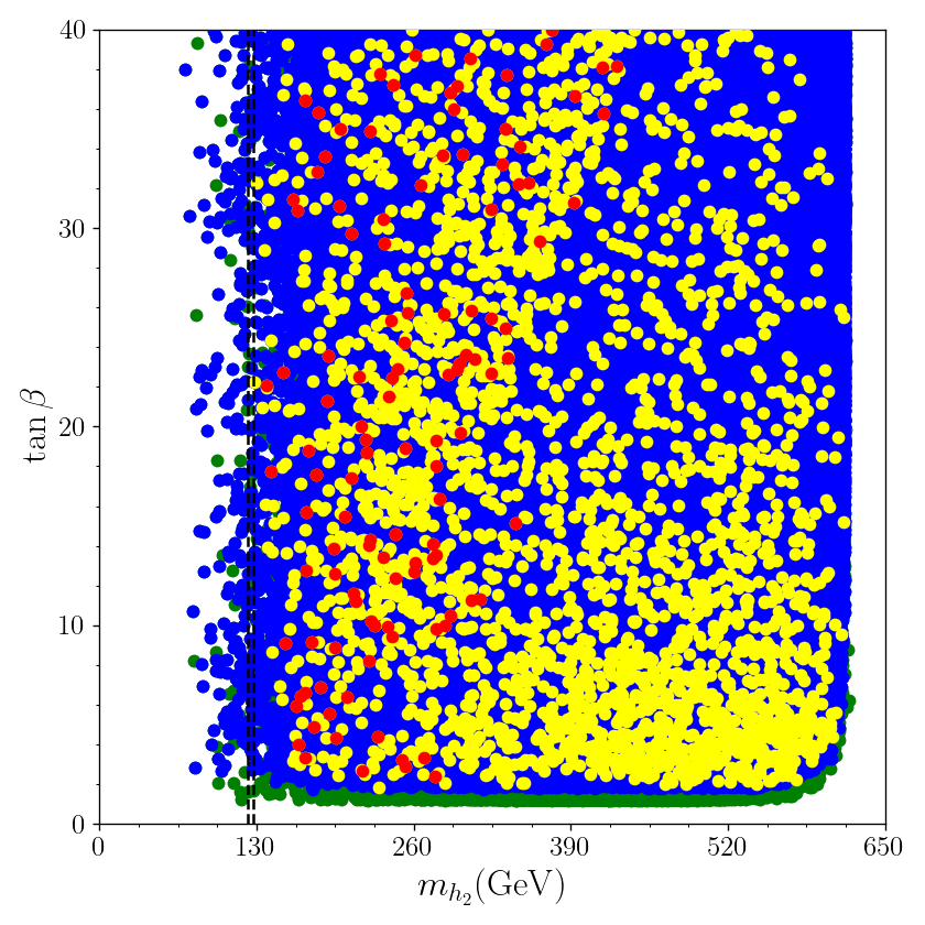
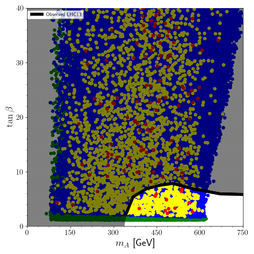
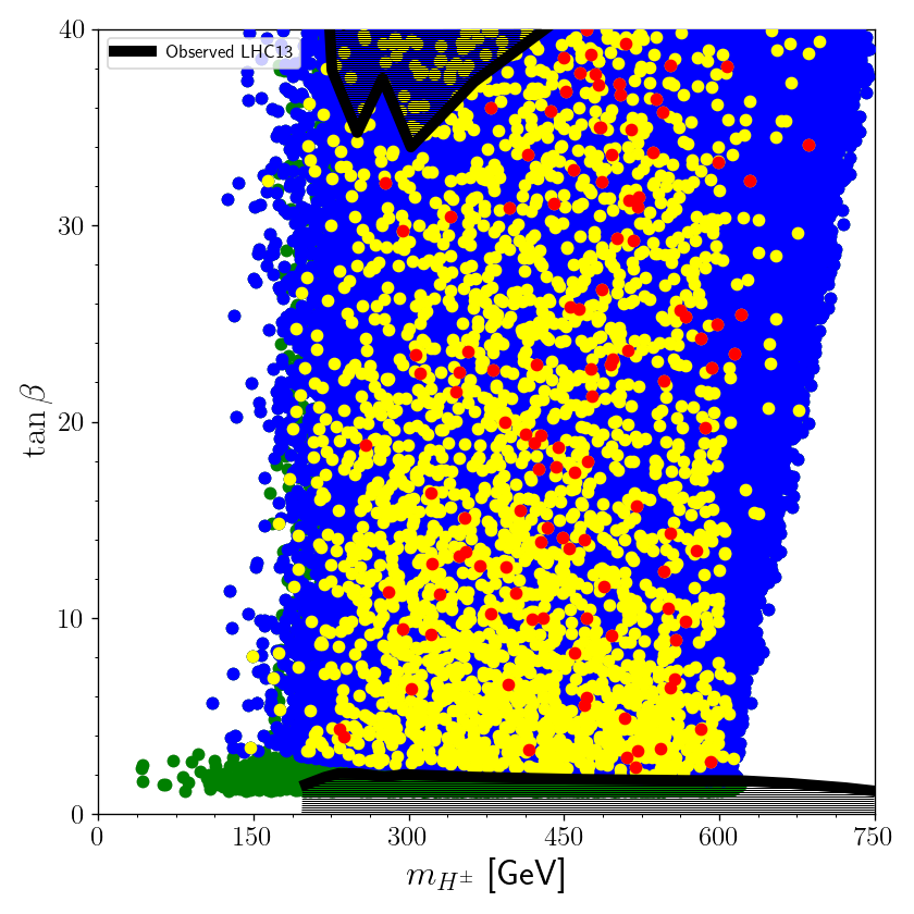
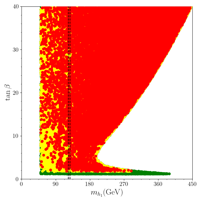
Figure 1: The relation between $\tan\beta$ and the mass of the LS-2HDM scalars, for $m_{h_{2}}$ (top-left), $m_{A}$ (top-right), $m_{H^{\pm}}$ (bottom-left) and $m_{h_{1}}$ (bottom-right). Color coding of solutions are described in detail in previous text and summarized as: Green points satisfy conditions G1, blue points satisfy conditions G1 and G2, yellow points satisfy conditions G1, G2 and G3, and red points satisfy conditions G1, G2, G3 and G4. Solid black lines indicate ATLAS 13 TeV analysis observation limits and gray shaded areas are excluded by these analysis [87, 88]. In $\tan\beta$ vs $m_{h_{1}}$ plot (bottom-right), condition G3 is not applied. Dashed vertical lines represent the SM Higgs mass.

First, the correlation between the masses of the LS-2HDM scalars and $\tan\beta$ are illustrated in Fig. 1. It is seen from Fig. 1 (top-left) that solutions satisfying the theoretical constraints specified by G1 do not introduce further limitations on $m_{h_{2}}$. The blue points in this plot represent solutions that meet both theoretical and experimental constraints specified in groups G1 and G2 within the ranges of $1.6\lesssim\tan\beta\lesssim 40.0$ and $70\lesssim m_{h_{2}}\lesssim 620$ GeV. It’s evident that the application of G2 does not result in a significant reduction of the parameter space. The yellow points signify solutions that additionally fulfill the condition $m_{h_{1}}=125\pm 2$ GeV (G1, G2, and G3). While the application of G3 does not restrict the range of $\tan\beta$, it does reduce the number of solutions in the parameter space, and imposes the condition $m_{h_{2}}\gtrsim 126$ GeV. The solutions indicated by the red points in Fig.1 (top-left) depict the parameter space that fulfills all four constraints outlined by groups G1, G2, G3, and G4, i.e. additionally satisfying restrictions coming from $M_{W}$, which limits the mass of the CP-even scalar boson as $135\lesssim m_{h_{2}}\lesssim 430$ GeV. The region between the vertical dashed lines in Fig. 1 (top-left) corresponds to the case where $h_{2}$ is the SM Higgs boson, which does not satisfy G4, i.e. W-boson mass condition. Therefore, the selection of $h_{1}$ as the SM Higgs boson, as specified in constraint G3, is clarified.

Additionally, the relationship between $m_{A}$ and $\tan\beta$ is depicted in Fig. 1 (top-right), together with the experimental constraints from ATLAS 13 TeV results, where $m_{A}$ span the full $60\lesssim m_{A}\lesssim 750$ GeV range. It is observed that the application of constraints G1 and G2 imposes limitations as $80\lesssim m_{A}\lesssim 600+4.1\tan\beta$ GeV. Moreover, adding the condition outlined as G3 reduces the number of solutions within the aforementioned regions. However, imposing W-mass constraints described as G4 require $100\lesssim m_{A}\lesssim 650$ GeV. The black line indicates the upper exclusion limit from ATLAS 13 TeV analysis [87], and it eliminates the majority of the solutions in the parameter space. Consequently, the solutions satisfying all constraints outlined as G1, G2, G3 and G4, and also imposing limits from ATLAS 13 TeV model independent scalar mass analysis, the mass of the CP-odd scalar boson and $\tan\beta$ are restricted as $330\;\text{GeV}\lesssim m_{A}\lesssim 600\;\text{GeV}~{}\text{and}\ \ \tan\beta\lesssim 8.0$. Based on these findings, low $\tan\beta$ region described here will be focused in the rest of this study. For the charged scalars of LS-2HDM, the variation of $m_{H^{\pm}}$ on the $\tan\beta-m_{H^{\pm}}$ plane is given in Fig. 1 (bottom-left). After applying constraints G1 and G2, the remaining solutions bounded as $110\ \text{GeV}\lesssim m_{H^{\pm}}\lesssim\ 605+3.8\tan\beta\ \text{GeV}$. However, after applying G3, the lower bound on $m_{H^{\pm}}$ increases to 150 GeV. After adding cuts from G4, the acceptable solutions satisfy $230\lesssim m_{H^{\pm}}\lesssim 685$ GeV, and number of valid solutions are reduced. The exculusion limits from ATLAS 13 TeV [88] requires $\tan\beta\geq 2.5$.

Until now, the CP-even scalar boson $h_{1}$ has been identified as the SM Higgs boson, and this requirement was described as condition G3. In order to explore the behavior of $m_{h_{1}}$, we remove condition G3, allowing $m_{h_{1}}$ to vary without constraints. The relationship between $\tan\beta$ and $m_{h_{1}}$, in this case, is presented in Fig. 1 (bottom-right). It is observed that $m_{h_{1}}$ exhibits distinct behavior in two specific regions of $\tan\beta$. For $\tan\beta\lesssim 5$, $m_{h_{1}}$ shows an inverse proportionality to $\tan\beta$, ranging from $50\lesssim m_{h_{1}}\lesssim 288$ GeV, where upper limit arises from condition G4. Conversely, for $\tan\beta\geq 5$, $m_{h_{1}}$ demonstrates a direct proportionality to $\tan\beta$, with values ranging as $50\lesssim m_{h_{1}}\lesssim 450$ GeV. This contrasting behavior in the low and high $\tan\beta$ regions is evident from Eqn. 5.

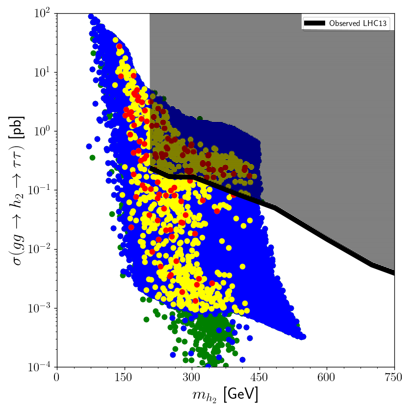
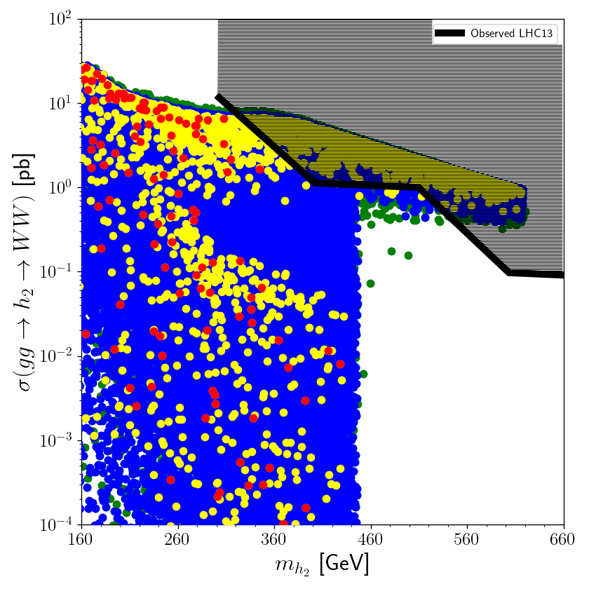
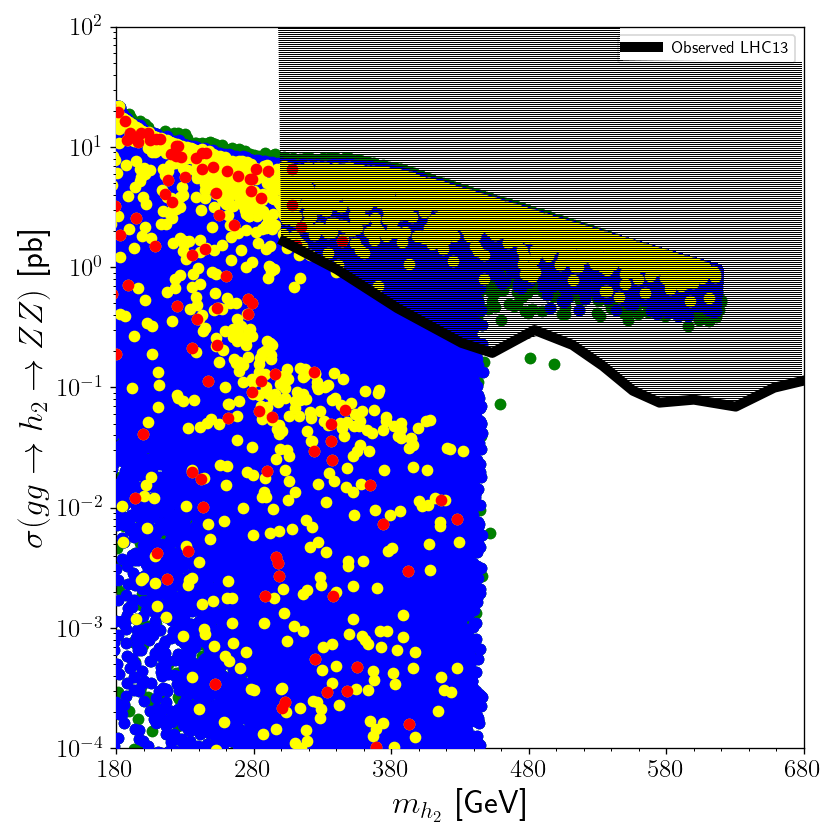
Figure 2: The variation of the cross-sections $\sigma(gg\rightarrow h_{2}\rightarrow\tau\tau)$ (top-left), $\sigma(gg\rightarrow h_{2}\rightarrow WW)$ (top-right) and $\sigma(gg\rightarrow h_{2}\rightarrow ZZ)$ (bottom) with respect to $m_{h_{2}}$. The color scheme is same as Fig. 1, and black shaded areas are excluded by Refs. [87, 89, 90]

Moreover, an analysis conducted by ATLAS at 13 TeV has established an upper limit on $m_{h_{2}}$ through various channels, including the decay modes of $h_{2}$ into two tau-leptons, two W-bosons, or two Z-bosons [87, 89, 90]. To investigate these limitations, the variation of the cross-sections $\sigma(gg\rightarrow h_{2}\rightarrow\tau\tau)$, $\sigma(gg\rightarrow h_{2}\rightarrow WW)$ and $\sigma(gg\rightarrow h_{2}\rightarrow ZZ)$ with respect to $m_{h_{2}}$ are depicted in Fig. 2. It is observed from Fig. 2 (top-left) that as $m_{h_{2}}$ increases, the production cross-section in channel $\sigma(gg\rightarrow h_{2}\rightarrow\tau\tau)$ decreases exponentially. According to the restrictions outlined in Ref. [87], nearly half of the solutions that satisfy criteria G4 are excluded, and the allowed parameter range necessitates $m_{h_{2}}\gtrsim 200$ GeV, along with $\sigma(gg\rightarrow h_{2}\rightarrow\tau\tau)\lesssim 2\times 10^{-1}$ pb. Observing Fig. 2 (top-right), it’s easily seen that the $\sigma(gg\rightarrow h_{2}\rightarrow WW)$ value decreases as $m_{h_{2}}$ increases, as expected. Importantly, the solutions that satisfy G4 remain unaffected by the constraint reported in Ref. [89]. For $m_{h_{2}}\gtrsim 450$ GeV, solutions with $\sigma(gg\rightarrow h_{2})\simeq 1.0$ pb and $BR(h_{2}\rightarrow WW)\simeq 1.0$ can be obtained. A similar behavior can be seen in Fig. 2 (bottom) where the dependence of $\sigma(gg\rightarrow h_{2}\rightarrow WW)$ on $m_{h_{2}}$ is plotted, the production cross-section decreases as $m_{h_{2}}$ increases. Although some solutions satisfying G4 are excluded by the constraints outlined in Ref. [90], it’s worth noting that for $m_{h_{2}}$ exceeding 450 GeV, the cross-section for the decay channel $\sigma(gg\rightarrow h_{2}\rightarrow ZZ)$ remains above 1 pb. After considering these findings from Fig.2, the mass of the heavier CP-even scalar boson is restricted as $164\lesssim m_{h_{2}}\lesssim 195$ GeV.

IV.2 Lepton Flavor Universality in Z-Boson Decay

The LS-2HDM makes a notable contribution to lepton universality through the inclusion of extra scalar bosons in the leptonic Yukawa couplings. Electroweak precision measurements conducted by LEP experiments, utilizing data from Z-boson resonances, estimate the ratio of decay widths as [79, 80]

$${\Gamma_{Z\to\mu^{+}\mu^{-}}\over\Gamma_{Z\to e^{+}e^{-}}} = 1.0009\pm 0.0028\,,$$ (16)

$${\Gamma_{Z\to\tau^{+}\tau^{-}}\over\Gamma_{Z\to e^{+}e^{-}}} = 1.0019\pm 0.0032\,.$$

Following this result, the contributions to the leptonic decays of the Z boson can be given as

$$\delta_{\mu\mu} = {\Gamma_{Z\to\mu^{+}\mu^{-}}\over\Gamma_{Z\to e^{+}e^{-}}}-1=(9\pm 28)\times 10^{-4},$$ (17)

$$\delta_{\tau\tau} = {\Gamma_{Z\to\tau^{+}\tau^{-}}\over\Gamma_{Z\to e^{+}e^{-}}}-1=(19\pm 32)\times 10^{-4},$$

where $\delta_{\mu\mu}$ and $\delta_{\tau\tau}$ are the parameters defined to measure the deviation from SM. The couplings of the Z-boson with fermions and extra scalar bosons are given as [80]

$$-{\cal L} ={g\over\cos\theta_{W}}Z^{\mu}\big{\{}\bar{f}\gamma_{\mu}(((T_{3}(f_{L})-Q(f_{L})\sin\theta_{W}^{2})\delta g_{L}^{\rm LS-2HDM})P_{L}+((T_{3}(f_{R})Q(f_{R})\sin\theta_{W}^{2})+\delta g_{R}^{\rm LS-2HDM})P_{R})f$$ (18)

$$+i(-{1\over 2}+\sin\theta_{W}^{2})H^{+}\overleftrightarrow{\partial_{\mu}}H^{-}+A\overleftrightarrow{\partial_{\mu}}H\big{\}}.$$

where, the contributions from LS-2HDM arise through $\delta g_{R,L}^{LS-2HDM}$. In the LS-2HDM, the loop contributions to the Z boson decay widths are expressed in terms of these parameters, and they are defined as

$$\delta g_{L}^{\rm 2HDM} =k\left[-\dfrac{1}{2}B_{Z}\left(r_{A}\right)-\dfrac{1}{2}B_{Z}\left(r_{h_{2}}\right)-2C_{Z}\left(r_{A},r_{h_{2}}\right)+\sin^{2}\theta_{W}\left(B_{Z}\left(r_{A}\right)+B_{Z}\left(r_{h_{2}}\right)+\tilde{C}_{Z}(r_{A})+\tilde{C}_{Z}(r_{h_{2}})\right)\right],$$ (19)

$$\delta g_{R}^{\rm 2HDM} =k\left[2C_{Z}\left(r_{A},r_{h_{2}}\right)-2C_{Z}\left(r_{H^{\pm}},r_{H^{\pm}}\right)+\tilde{C}_{Z}(r_{H^{\pm}})-\dfrac{1}{2}\tilde{C}_{Z}(r_{A})-\dfrac{1}{2}\tilde{C}_{Z}(r_{h_{2}})\right.,$$

$$+\left.\sin^{2}\theta_{W}\left(B_{Z}\left(r_{A}\right)+B_{Z}\left(r_{h_{2}}\right)+2B_{Z}\left(r_{H^{\pm}}\right)+\tilde{C}_{Z}(r_{A})+C_{Z}\left(r_{H^{\pm}},r_{H^{\pm}}\right)\right)\right],$$

where, $k=m_{f}^{2}\tan^{2}\beta/16\pi^{2}v^{2}$, $m_{f}$ are fermion masses, $\Lambda$ is the cut-off scale, $\mu$ is the renormalization scale, and $r_{\phi}=m_{\phi}^{2}/m_{Z}^{2}$ ($\phi=A,h_{2},H^{\pm}$). The loop functions employed in Eqn. 19 are calculated as

$$B_{Z}(r) =-\dfrac{1}{2}\left(\ln\Lambda^{2}+\log(4\pi)\right)-\dfrac{1}{4}+\dfrac{1}{2}\log r,$$ (20)

$$\tilde{C}_{Z}(r) =-\dfrac{1}{2}\left(\ln\Lambda^{2}+\log(4\pi)\right)-\dfrac{1}{2}-r\left(1+\log r\right)+r^{2}\left(\log r\log(1+r^{-1})-{\rm dilog}(-r^{-1})\right)$$

$$-\dfrac{i\pi}{2}\left(1-2r+2r^{2}\log\left(1+r^{-1}\right)\right),$$

$$C_{Z}\left(r_{1},r_{2}\right) =C_{Z}(\dfrac{m_{\phi_{1}}^{2}}{m_{Z}^{2}},\dfrac{m_{\phi_{2}}^{2}}{m_{Z}^{2}})=C_{00}(0,0,m_{Z}^{2},m_{\phi_{1}}^{2},m_{\phi_{2}}^{2}),$$

$$C_{00} =\dfrac{1}{4}\left(\ln\Lambda^{2}+\log(4\pi)-\ln(\dfrac{m_{Z}^{2}}{\mu^{2}})\right)+\dfrac{3}{8}-\dfrac{r_{1}^{2}\ln r_{1}}{4(r_{1}-1)(r_{1}-r_{2})}+\dfrac{r_{2}^{2}\ln r_{2}}{4(r_{2}-1)(r_{1}-r_{2})}.$$

The parameters defined in Eqn. 17 can be related to $\delta g_{R,L}^{LS-2HDM}$ appearing in Eqn. 18 as

$$\delta_{ll}={2g_{L}^{e}{\rm Re}(\delta g^{\rm LS-2HDM}_{L})+2g_{R}^{e}{\rm Re}(\delta g^{\rm LS-2HDM}_{R})\over{g_{L}^{e}}^{2}+{g_{R}^{e}}^{2}},$$ (21)

where $l=\mu,\tau$. Throughout this analysis, lepton universality in the Z-boson decay are investigated through parameters given in Eqn. 21.

In order to understand the impact of LS-2HDM on lepton universality, such as the loop-induced contributions to the Z boson decay widths, it’s essential to explore the precise measurements of lepton universality ratios provided in Eqn. 16 within the framework of LS-2HDM. To this end, the distribution of solutions that satisfy the constraints outlined as G1, G2, G3 and G4 are plotted on $\delta_{ll}$ and $\tan\beta$ plane in left for $\delta_{\mu\mu}$ and in right for $\delta_{\tau\tau}$, in Figure 3.

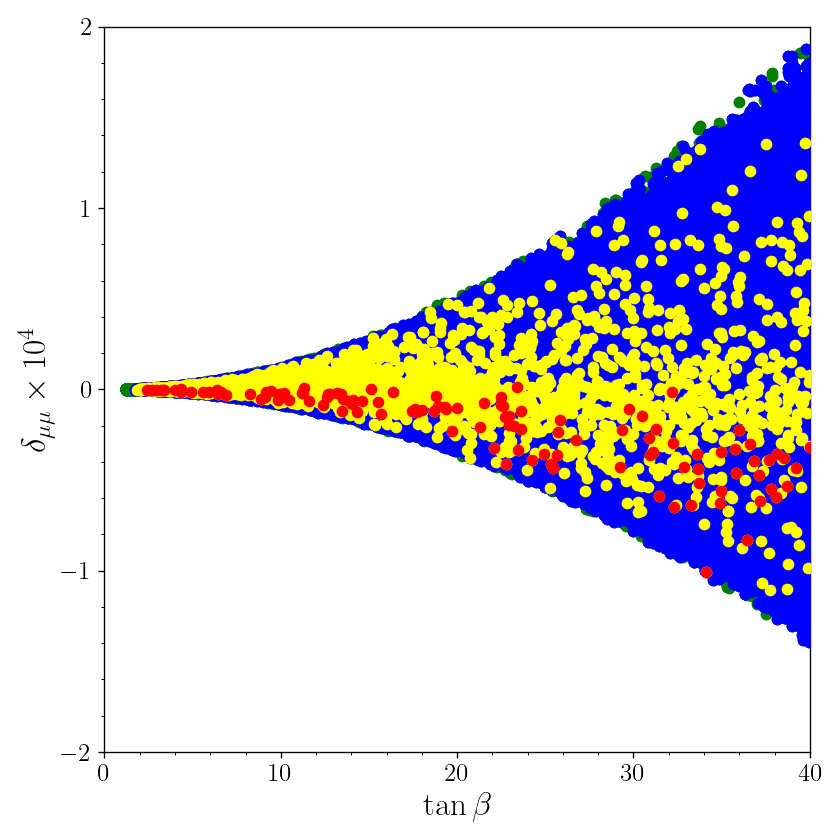
Figure 3: The variation of $\delta_{\mu\mu}$ with respect to $\tan\beta$ (left) and $\delta_{\tau\tau}$ with respect to $\tan\beta$ (right). Color coding of the plots is the same as Fig. 1. The dashed, dotted and solid lines indicate deviations from the current limits by Eqn. 17 within $1\sigma$, $2\sigma$, and $3\sigma$, respectively. For $\delta_{\mu\mu}$ (left), all solutions lie within 1$\sigma$ vicinity.

It is seen from Fig. 3 that the dependence of $\delta_{ll}$ on $\tan\beta$ is quadratic as indicated in Eqn. 19, in both positive or negative directions depending on the scalar masses of the LS-2HDM. Moreover, Fig. 3 (left) demonstrates that the deviation of $\delta_{\mu\mu}$ from the SM prediction lies within $1\sigma$ level and increases with the $\tan\beta$. Notably, to satisfy the W-boson mass constraint given by G4, the value of $\delta_{\mu\mu}$ must be negative. Furthermore, Fig. 3 (right) demonstrates that $\delta_{\tau\tau}$ displays a greater sensitivity to $\tan\beta$, due to the contribution of $m_{\tau}^{2}$. It is important to note that the contribution can be either positive or negative, but if the parameter space is restricted by G4, $\delta_{\tau\tau}$ is typically negative with a few exceptions. The majority of solutions satisfying all constraints—G1, G2, G3, and G4—are observed to fall within a $3\sigma$ deviation from the observed value of $\delta_{\tau\tau}=1.0019$.

To understand the behavior of $\delta_{\tau\tau}$, three solutions represented by the red points from the $\delta_{\tau\tau}$ - $\tan\beta$ plane in Fig. 3(right), satisfying all the constraints, are selected. Corresponding scalar masses, alongside $\Delta M_{W}=M_{W}^{\rm LS-2HDM}-M_{W}^{\rm SM}$ —representing the deviation of the W-boson mass in LS-2HDM from its SM value— are detailed in Table 2. As can be seen from the Table 2 that $m_{h_{2}}$ and $m_{H^{\pm}}$ increase with $\delta_{\tau\tau}$. Although there isn’t an explicit linear correlation between $m_{A}$ and $\delta_{\tau\tau}$, an increase in $\delta_{\tau\tau}$ can result in higher values of $m_{A}$. It can also be seen from Eqn. 5 that, when $m_{3}^{2}$ and $\lambda_{3}$ are negative, $m_{A}$ and $m_{H^{\pm}}$ increase with $\tan\beta$. In Table 2, the value of $\Delta M_{W}$ at chosen solutions are also given, which does not exhibit significant dependence on alterations within the parameter space.

$\delta_{\tau\tau}$	$-0.9929\times 10^{-4}\;(1\sigma)$	$-26.1088\times 10^{-4}\;(2\sigma)$	$-61.6004\times 10^{-4}\;(3\sigma)$
$\tan\beta$	$3.3094$	$18.903$	$23.623$
$m_{h_{1}}$	$125.164$	$123.095$	$124.39$
$m_{h_{2}}$	$169.964$	$253.095$	$303.058$
$m_{A}$	$388.266$	$382.756$	$479.669$
$m_{H^{\pm}}$	$416.205$	$421.037$	$511.855$
$\Delta M_{W}$	$0.0533$	$0.0539$	$0.0536$

Table 2: Properties of solutions which are selected from Fig. 3 (right). All masses and $\Delta M_{W}^{\prime}$ are given in GeV unit. $1\sigma,2\sigma,3\sigma$ are the deviations from value of $\delta_{\tau\tau}$ (1.0019).

IV.3 Lepton Flavor Universality in Tau Decay

Following the analysis in previous section, the behaviour of LFU in tau decays within LS-2HDM is also investigated. At the loop-level, the LFU in tau decay gets contributions from the LS-2HDM scalars, and these contributions bring additional constraints on the parameter space of the LS-2HDM. The ratio of these couplings are defined as

$$\left(g_{\tau}\over g_{\mu}\right)=1+\delta_{\rm loop},\qquad\left(g_{\tau}\over g_{e}\right)=1+\delta_{\rm tree}+\delta_{\rm loop},\qquad\left(g_{\mu}\over g_{e}\right)=1+\delta_{\rm tree},$$ (22)

where $\delta_{\rm loop}$ and $\delta_{\rm tree}$ are the contributions to SM value from loop and tree level processes. In LS-2HDM, these contributions are calculated as [85, 80, 81]

$$\delta_{\rm tree} ={m_{\tau}^{2}m_{\mu}^{2}\over 8m^{4}_{H^{\pm}}}t^{4}_{\beta}-{m_{\mu}^{2}\over m^{2}_{H^{\pm}}}t^{2}_{\beta}{g(m_{\mu}^{2}/m^{2}_{\tau})\over f(m_{\mu}^{2}/m_{\tau}^{2})},$$ (23)

$$\delta_{\rm loop} ={1\over 16\pi^{2}}{m_{\tau}^{2}\over v^{2}}t^{2}_{\beta}\left[1+{1\over 4}\left(H(m_{A}^{2}/m_{H^{\pm}}^{2})+s^{2}_{\beta-\alpha}H(m_{h_{2}}^{2}/m_{H^{\pm}}^{2})+c^{2}_{\beta-\alpha}H(m_{h_{1}}^{2}/m_{H^{\pm}}^{2}\right)\right],$$

where

$$f(x) \equiv 1-8x+8x^{3}-x^{4}-12x^{2}\ln(x),$$

$$g(x) \equiv 1+9x-9x^{2}-x^{3}+6x(1+x)\ln(x),$$ (24)

$$H(x) \equiv\ln(x)(1+x)/(1-x),$$

and $t_{\beta}=\tan\beta$, $s_{\beta-\alpha}=\sin(\beta-\alpha)$, $c_{\beta-\alpha}=\cos(\beta-\alpha)$ are defined for brevity. Using pure leptonic processes, HFLAV collaboration obtained the values of the ratios given in Eqn. 23 as [86]

$$\left(g_{\tau}\over g_{\mu}\right)=1.0009\pm 0.0014,\qquad\left(g_{\tau}\over g_{e}\right)=1.0027\pm 0.0014,\qquad\left(g_{\mu}\over g_{e}\right)=1.0019\pm 0.0014.$$ (25)

These averages define the ranges for loop and tree-level contributions as

$$\delta_{loop}=0.0009\pm 0.0014~{}\ \ \text{and}\ \ \ \ \delta_{tree}=0.0019\pm 0.0014~{},$$ (26)

and these limits will be considered for further analysis.

Figure 4: $\delta_{loop}$ vs $\tan\beta$ (left), and $\delta_{tree}$ vs $\tan\beta$ (right). Color coding is the same as Fig. 1. All solutions lay within the $1\sigma$ vicinity of HFLAV results.

To examine the relationship between solutions satisfying all four constraints, they are plotted in the $\delta_{loop}$ and $\delta_{tree}$ versus $\tan\beta$ planes in Fig. 4 (left and right), respectively. It is observed from Fig. 4 that applying constraints reduces the number of solutions, and restricts them in negative plane. Furthermore, all solutions shown in red in Fig. 4 (left) lie within $2\sigma$ vicinity of the HFVAL average value of $\delta_{loop}$ given in Eqn. 26. Remarkably, for solutions with $\tan\beta<20$, this proximity is confined within the 1$\sigma$ range. On the other hand, concerning $\delta_{tree}$, solutions meeting all constraints are clustered just below zero, confined within a $1\sigma$ to $2\sigma$ window of the average value, as observed in Fig. 4 (right). Finally, it is also apparent from Fig. 4 that with increasing $\tan\beta$, loop contributions to the ratios from LS-2HDM become more significant in comparison to those at the tree level.

IV.4 W-Boson Mass in LS-2HDM

As previously noted, the CDF collaboration has recently reported a new measurement of the W-boson mass, deviating by 7$\sigma$ from the prediction of the SM, as given in Eqn.1. This section aims to investigate whether the LS-2HDM framework can provide solutions compatible with both experimental and theoretical limitations outlined as G1 and G2, while allowing for a deviation of $3\sigma$ from the reported W-boson mass by CDF. Specifically, the behavior of the W-boson mass within the framework of LS-2HDM will be investigated.

In the context of the LS-2HDM, the W-boson mass can be calculated as

[111]

$$M_{W}^{2}={M_{W}^{\rm SM}}^{2}\left(1+\frac{s_{W}^{2}}{c_{W}^{2}-s_{W}^{2}}\Delta r^{\prime}\right)\ ,$$ (27)

where

$$\Delta r^{\prime}=\frac{\alpha}{s_{W}^{2}}\left(-\frac{1}{2}S+c_{W}^{2}T+\frac{c_{W}^{2}-s_{W}^{2}}{4s_{W}^{2}}U\right)\ ,$$ (28)

represents the measure of deviations from SM, and where $s_{W}=\sin\theta_{W}$ and $c_{W}=\cos\theta_{W}$ with $\theta_{W}$ is being the weak angle. In Eqn. 28, $S$, $T$, and $U$ represent the oblique parameters, containing the effects of incorporation of additional scalar bosons contributions through loops within the LS-2HDM framework to $M_{W}$. These parameters are defined based on precision measurements in electroweak physics, and in SM, $S=T=U=0$ serves as the reference point. The explicit form of the $S$, $T$, $U$ parameters are given as [112]

$$S= \frac{1}{\pi m_{Z}^{2}}\left\{-\mathcal{B}_{22}\left(m_{Z}^{2};m_{H^{\pm}}^{2},m_{H^{\pm}}^{2}\right)+\sin^{2}(\beta-\alpha)\mathcal{B}_{22}\left(m_{Z}^{2};m_{h_{2}}^{2},m_{A}^{2}\right)\right.$$ (29)

$$+\cos^{2}(\beta-\alpha)\left[\mathcal{B}_{22}\left(m_{Z}^{2};m_{h_{1}}^{2},m_{A}^{2}\right)+\mathcal{B}_{22}\left(m_{Z}^{2};m_{Z}^{2},m_{h_{2}}^{2}\right)-\mathcal{B}_{22}\left(m_{Z}^{2};m_{Z}^{2},m_{h_{1}}^{2}\right)\right.$$

$$\left.\left.-m_{Z}^{2}\mathcal{B}_{0}\left(m_{Z}^{2};m_{Z}^{2},m_{h_{2}}^{2}\right)+m_{Z}^{2}\mathcal{B}_{0}\left(m_{Z}^{2};m_{Z}^{2},m_{h_{1}}^{2}\right)\right]\right\},$$

$$T= \frac{1}{16\pi s_{W}^{2}m_{W}^{2}}\left\{\mathcal{F}\left(m_{H^{\pm}}^{2},m_{A}^{2}\right)+\sin^{2}(\beta-\alpha)\left[\mathcal{F}\left(m_{H^{\pm}}^{2},m_{h_{2}}^{2}\right)-\mathcal{F}\left(m_{A}^{2},m_{h_{2}}^{2}\right)\right]\right.$$ (30)

$$+\cos^{2}(\beta-\alpha)\left[\mathcal{F}\left(m_{H^{\pm}}^{2},m_{h_{1}}^{2}\right)-\mathcal{F}\left(m_{A}^{2},m_{h_{1}}^{2}\right)+\mathcal{F}\left(m_{W}^{2},m_{h_{2}}^{2}\right)-\mathcal{F}\left(m_{W}^{2},m_{h_{1}}^{2}\right)\right.$$

$$-\mathcal{F}\left(m_{Z}^{2},m_{h_{2}}^{2}\right)+\mathcal{F}\left(m_{Z}^{2},m_{h_{1}}^{2}\right)+4m_{Z}^{2}B_{0}\left(0;m_{Z}^{2},m_{h_{2}}^{2}\right)-4m_{Z}^{2}B_{0}\left(0;m_{Z}^{2},m_{h_{1}}^{2}\right)$$

$$\left.\left.-4m_{W}^{2}B_{0}\left(0;m_{W}^{2},m_{h_{2}}^{2}\right)+4m_{W}^{2}B_{0}\left(0;m_{W}^{2},m_{h_{1}}^{2}\right)\right]\right\},$$

$$S+U= \frac{1}{\pi m_{W}^{2}}\left\{\mathcal{B}_{22}\left(m_{W}^{2};m_{H^{\pm}}^{2},m_{A}^{2}\right)-2\mathcal{B}_{22}\left(m_{W}^{2};m_{H^{\pm}}^{2},m_{H^{\pm}}^{2}\right)+\sin^{2}(\beta-\alpha)\mathcal{B}_{22}\left(m_{W}^{2};m_{H^{\pm}}^{2},m_{h_{2}}^{2}\right)\right.$$ (31)

$$+\cos^{2}(\beta-\alpha)\left[\mathcal{B}_{22}\left(m_{W}^{2};m_{h_{1}}^{2},m_{H^{\pm}}^{2}\right)+\mathcal{B}_{22}\left(m_{W}^{2};m_{W}^{2},m_{h_{2}}^{2}\right)-\mathcal{B}_{22}\left(m_{W}^{2};m_{W}^{2},m_{h_{1}}^{2}\right)\right.$$

$$\left.\left.+m_{W}^{2}\mathcal{B}_{0}\left(m_{W}^{2};m_{W}^{2},m_{h_{2}}^{2}\right)-m_{W}^{2}\mathcal{B}_{0}\left(m_{W}^{2};m_{W}^{2},m_{h_{1}}^{2}\right)\right]\right\},$$

where

$$\mathcal{B}_{22}\left(q^{2};m_{1}^{2},m_{2}^{2}\right)\equiv\mathcal{B}_{22}\left(q^{2};m_{1}^{2},m_{2}^{2}\right)-\mathcal{B}_{22}\left(0;m_{1}^{2},m_{2}^{2}\right),$$ (32)

$$\mathcal{B}_{0}\left(q^{2};m_{1}^{2},m_{2}^{2}\right)\equiv\mathcal{B}_{0}\left(q^{2};m_{1}^{2},m_{2}^{2}\right)-\mathcal{B}_{0}\left(0;m_{1}^{2},m_{2}^{2}\right),$$

are the loop functions arising from two-point loop integrals given as

$$B_{22}\left(q^{2};m_{1}^{2},m_{2}^{2}\right)=\frac{1}{4}(\Delta+1)\left[m_{1}^{2}+m_{2}^{2}-\frac{1}{3}q^{2}\right]-\frac{1}{2}\int_{0}^{1}dxX\ln(X-i\epsilon),$$ (33)

$$B_{0}\left(q^{2};m_{1}^{2},m_{2}^{2}\right)=\Delta-\int_{0}^{1}dx\ln(X-i\epsilon),$$

where

$$X\equiv m_{1}^{2}x+m_{2}^{2}(1-x)-q^{2}x(1-x),\quad\Delta\equiv\frac{2}{4-d}+\ln 4\pi-\gamma.$$ (34)

Shorthand notation $\mathcal{F}$ in Eqn. 30 is defined as

$$\mathcal{F}\left(m_{1}^{2},m_{2}^{2}\right)\equiv\dfrac{1}{2}\left(m_{1}^{2}+m_{2}^{2}\right)-\dfrac{m_{1}^{2}m_{2}^{2}}{m_{1}^{2}-m_{2}^{2}}\ln\left(\dfrac{m_{1}^{2}}{m_{2}^{2}}\right),$$ (35)

satisfying the following relations

$$\mathcal{F}\left(m_{1}^{2},m_{2}^{2}\right)=\mathcal{F}\left(m_{2}^{2},m_{1}^{2}\right)\;{\rm and}\;\mathcal{F}\left(m^{2},m^{2}\right)=0.$$ (36)

To this end, one-loop contributions to both the oblique parameters and the W-boson mass in LS-2HDM are computed. To constrain the solutions, $M_{W}^{\rm LS-2HDM}$ is restricted to fall within a $3\sigma$ range of $M_{W}^{\rm CDF}$, namely $M_{W}^{\rm LS-2HDM}=80.4335\pm 3\times 0.0094$ GeV, resulting in the value of $\Delta M_{W}$ as

$$\Delta M_{W} =80.4335{\rm GeV}-80.357{\rm GeV}=0.0765\;{\rm GeV},$$ (37)

which provides the intervals given in Table 3.

	$\Delta M_{\rm W}^{\rm min}$	$\Delta M_{\rm W}^{\rm max}$
$1\sigma$	0.0671	0.0859
$2\sigma$	0.0577	0.0953
$3\sigma$	0.0483	0.1047

Table 3: Limits on $\Delta M_{W}$. All masses are in GeV.

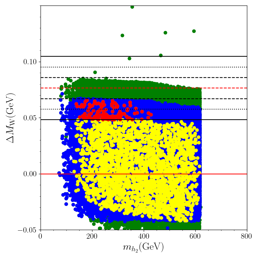
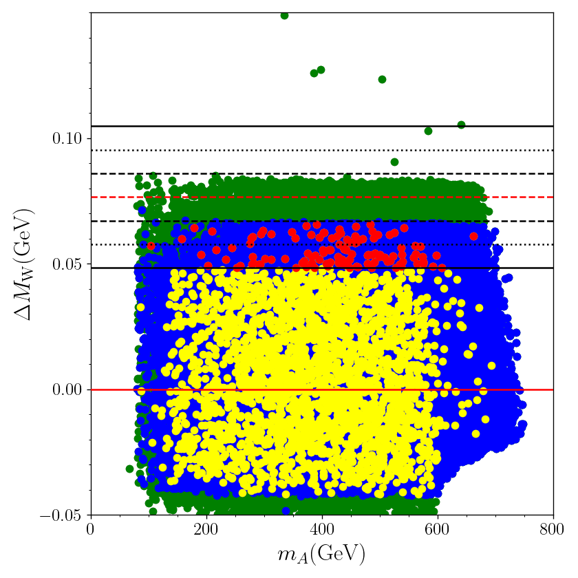
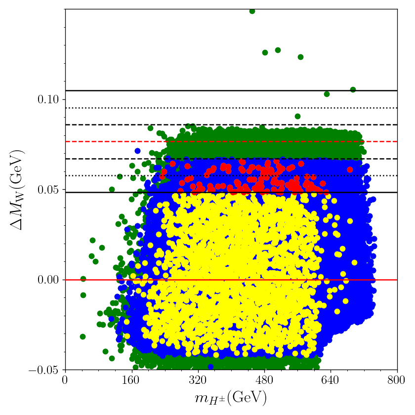
Figure 5: Solutions satisfying conditions G1, G2, G3 and G4 plotted in the $\Delta M_{W}$ versus $m_{h_{1}}$ (top-left), $m_{h_{2}}$ (top-right), $m_{A}$ (bottom-left), and $m_{H^{\pm}}$ (bottom-right). Color coding of the points is the same as Fig. 1. The solid and dashed red lines represent the deviations from SM and CDF-reported value, respectively. The dashed, dotted and solid lines indicate deviations from $M_{W}^{CDF}$ given in Table 3 within $1\sigma$, $2\sigma$, and $3\sigma$, respectively. In $\Delta M_{W}$ vs $m_{h_{1}}$ plot (top-left), constraint G3 is not applied.

Following these considerations, a thorough analysis of the parameters within the LS-2HDM that meet both the theoretical and experimental constraints outlined as G1, G2, and G3 is performed. The relations between the masses of LS-2HDM scalars and $\Delta M_{W}$ are depicted in Fig. 5. In the top-left panel of Fig. 5, the plot illustrates the relation between $\Delta M_{W}$ and $m_{h_{1}}$, where $m_{h_{1}}$ is not restricted to be SM for these solutions. For the new scalars in LS-2HDM, the solutions are plotted on the $\Delta M_{W}$ vs $m_{h_{2}}$, $m_{A}$, and $m_{H^{\pm}}$ planes in Fig. 5. From these plots, it can be concluded that assuming $h_{1}$ as SM Higgs boson predicts $\Delta M_{W}$ within $1\sigma$ to $3\sigma$ uncertainity, hence it is viable, and the masses of new scalars are restricted to be $140\lesssim m_{h_{2}}\lesssim 430$ GeV, $230\lesssim m_{H^{\pm}}\lesssim 685$ GeV, and $105\lesssim m_{A}\lesssim 665$ GeV.

Fig. 6 display the solutions for $\Delta M_{W}$ in correlation with $\tan\beta$, $m_{h_{2}}-m_{h_{1}}$, $m_{A}-m_{h_{2}}$, and $m_{H^{\pm}}-m_{A}$ planes. Observing Fig. 6 (top-left), it is seen that the viable solutions do not limit $\tan\beta$, and the contributions from LS-THDM to the W-boson mass generally exhibit positivity. However, the imposition of constraints grouped under G1 necessitates that $\tan\beta$ must exceed 2. Furthermore, it is noticeable that the W-boson mass aligns with predictions within the framework of the model. However, imposing condition G3, which assumes $h_{1}$ as the SM Higgs boson, restricts the deviation of $\Delta M_{W}$ to within the $1\sigma$ to $3\sigma$ range of the CDF-reported value but fails to predict results closer to it. This discrepancy might suggest a potential tension between $h_{1}$ being SM-like and $M_{W}^{\rm CDF}$ in the LS-2HDM framework. Furthermore, it is observed from Fig. 6 (top-right) that the W-boson mass can be obtained in LS-2HDM by imposing the constriant for the mass difference between the CP-even scalar bosons as $20\lesssim m_{h_{2}}-m_{h_{1}}\lesssim 300$ GeV. Similarly, the mass difference between pseudoscalar and heavy scalar bosons can take values in between the range $-125\lesssim M_{A}-m_{h_{2}}\lesssim 425$ GeV. Finally, in Fig. 6 (bottom-right), it is observed that the restricted range for the mass difference between charged scalars and pseudoscalar states is $15\lesssim m_{H^{\pm}}-m_{A}\lesssim 127$ GeV. Notably, the relationship between $\Delta M_{W}$ and $m_{H^{\pm}}-m_{A}$ differs due to the dependence of $m_{H^{\pm}}-m_{A}$ on the oblique parameters $S$, $T$ and $U$.

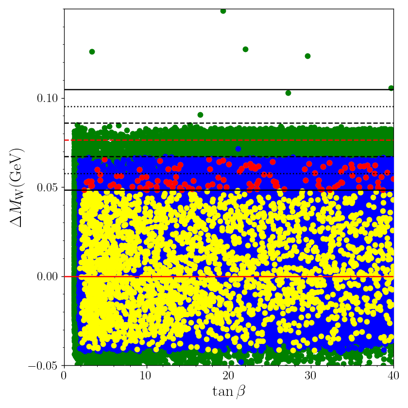
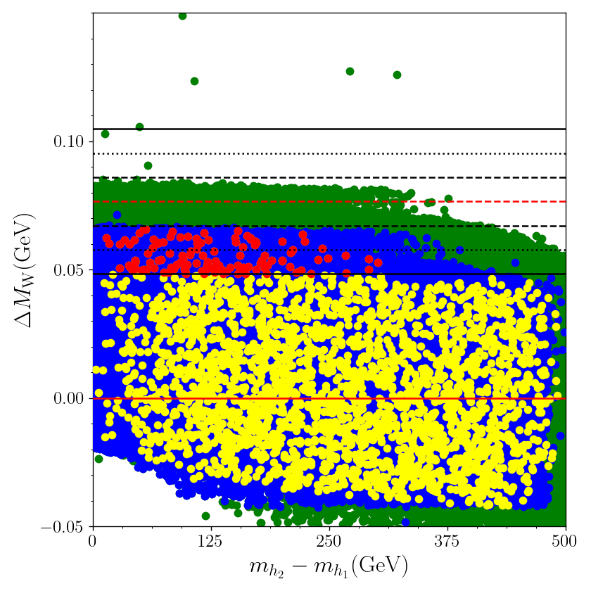
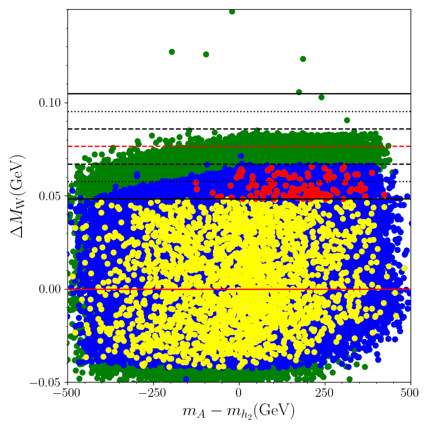
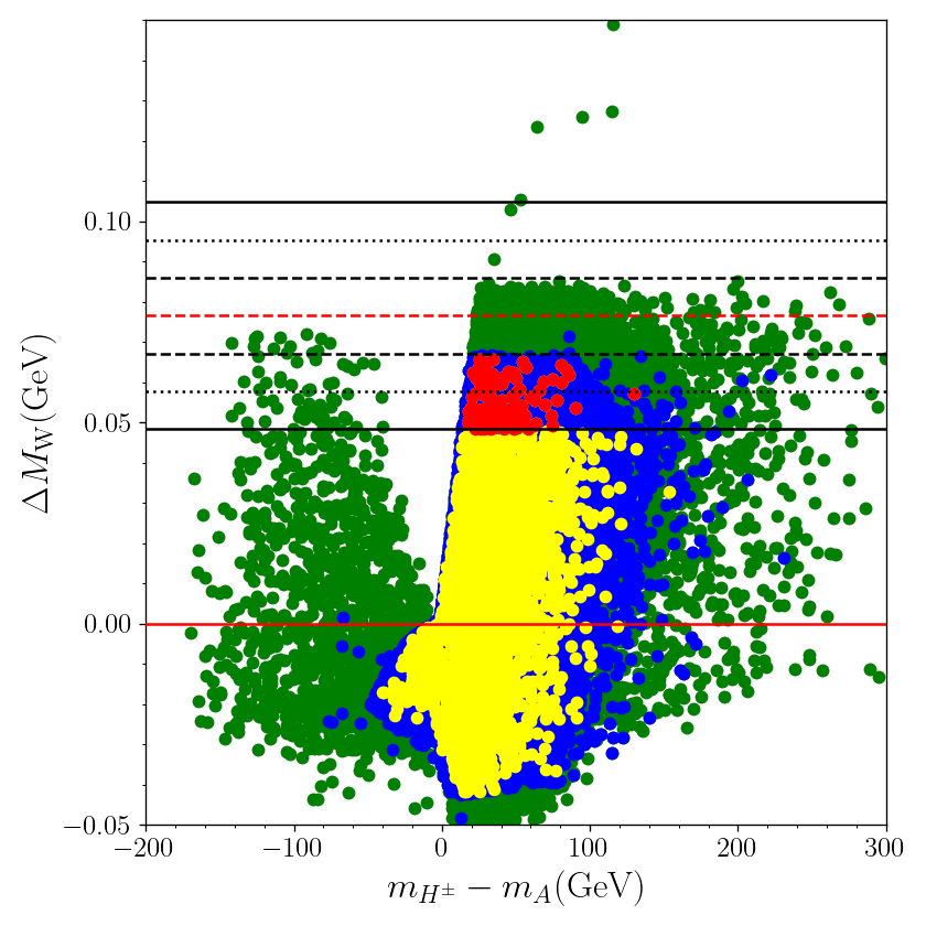
Figure 6: Solutions satisfying conditions G1, G2, G3 and G4 plotted in the $\Delta M_{W}$ versus $\tan\beta$ (top-left), $m_{h_{2}}-m_{h_{1}}$ (top-right), $m_{A}-m_{h_{2}}$ (bottom-left), and $m_{H^{\pm}}-m_{A}$ (bottom-right). Color coding of the points is the same as Fig. 1. The solid and dashed red lines represent the deviations from SM and CDF-reported value, respectively. The dashed, dotted and solid lines indicate deviations from $M_{W}^{CDF}$ given in Table 3 within $1\sigma$, $2\sigma$, and $3\sigma$, respectively.

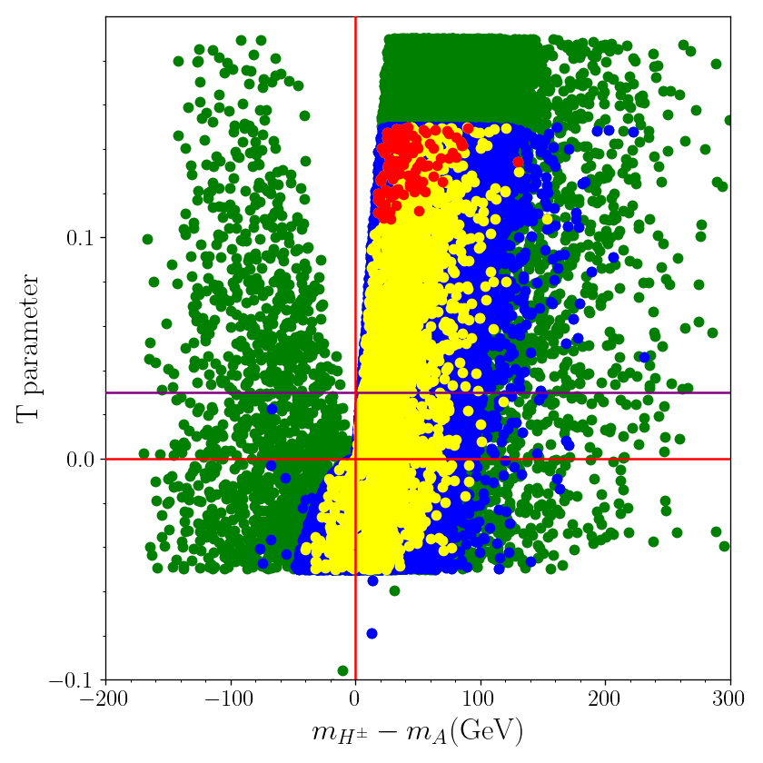
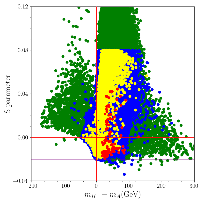
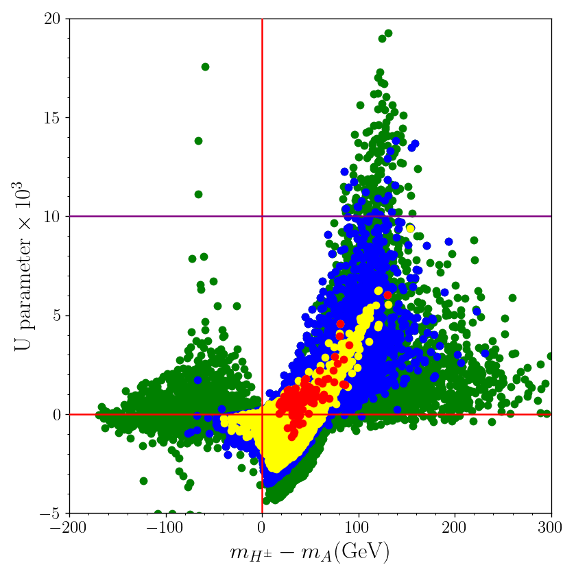
Figure 7: Solutions satisfying all four limitations plotted in $T$ vs $m_{H^{\pm}}-m_{A}$ (top-left), $S$ vs $m_{H^{\pm}}-m_{A}$ (top-right), and $U$ vs $m_{H^{\pm}}-m_{A}$ (bottom). Color coding of the points is the same as Fig. 1. Solid purple lines indicates the values given in Eq. 13. Vertical and horizontal solid red lines represent zero values.

Fig. 7 illustrates the impacts of the oblique parameters in correlation with the mass difference in $T$ vs $m_{H^{\pm}}-m_{A}$ (top-left), $S$ vs $m_{H^{\pm}}-m_{A}$ (top-right), and $U$ vs $m_{H^{\pm}}-m_{A}$ (bottom). Solutions that satisfy all four sets of constraints estimate the $T$, $S$, and $U$ oblique parameters within the $1\sigma$ vicinity, as described by Eqn. 13. Notably, Fig. 7 (right) demonstrates a similar trend to the plots depicting the behavior of the $S$, $T$, and $U$ parameters. However, the influence of parameter $T$ on $\Delta M_{W}$ appears to be predominant. Finally, these solutions specify the following ranges

$$0.1\; \lesssim\;T\;\lesssim 0.15\ ,$$

$$-0.02\; \lesssim\;S\;\lesssim 0.045\ ,$$

$$-1.10\times 10^{-3}\; \lesssim\;U\;\lesssim 6.05\times 10^{-3}\ ,$$ (38)

within which $M_{W}^{CDF}$ can be obtained within the $1\sigma$ to $3\sigma$ vicinity.

IV.5 Further Analysis

In this section, all results discussed in previous sections will be summarized. In addition, benchmark points and their properties will be given. Finally, all obtained solutions will be tested in HiggsTools package [92].

Parameter	Minimum Value	Maximum Value
$m_{h_{2}}-m_{h_{1}}$	$20$	$300$
$m_{H^{\pm}}-m_{A}$	$15$	$127$
$m_{A}-m_{h_{2}}$	$-125$	$425$
$m_{h_{2}}$	$164$	$195$
$m_{A}$	$330$	$575$
$m_{H^{\pm}}$	$345$	$685$
$\tan\beta$	$2.5$	$8.0$
$T$	$0.1$	$0.15$
$S$	$-0.02$	$0.045$
$U$	$-1.1\times 10^{-3}$	$6.05\times 10^{-3}$

Table 4: The constraints on the model parameters which satisfy all four aforementioned group of limitations. All masses are given in GeV unit.

The properties of solutions satisfying all for constraints listed before as G1, G2, G3 and G4, are given in Table 4. Within these ranges, $0.0483\lesssim\Delta M_{W}\lesssim 0.0671$ GeV, i.e. LS-2HDM can estimate the mass of the W boson as

$$80.4053\lesssim M_{W}^{LS-2HDM}\lesssim 80.4147\ \text{GeV}.$$ (39)

Among these solutions, three points closely estimating $M_{W}^{LS-2HDM}$ around the Standard Model value, and an additional three points estimating $M_{W}^{LS-2HDM}$ around the CDF-reported value, have been selected as benchmarks. Their respective properties are detailed in Table 5.

Parameter	1. Point	2. Point	3. Point	4. Point	5. Point	6. Point
$M_{W}^{\rm LS-2HDM}$	$80.3569$	$80.3589$	$80.3514$	$80.4240$	$80.4236$	$80.4234$
Deviation from $M_{W}^{\rm CDF}$	$8.06\sigma$	$7.85\sigma$	$8.64\sigma$	$1.01\sigma$	$1.04\sigma$	$1.05\sigma$
$m_{h_{1}}$	$126.708$	$125.883$	$123.418$	$124.079$	$124.096$	$124.902$
$m_{h_{2}}$	$176.646$	$497.022$	$595.514$	$281.157$	$372.323$	$250.747$
$m_{A}$	$426.245$	$292.904$	$136.475$	$208.244$	$190496$	$530.388$
$m_{H^{\pm}}$	$426.245$	$343.396$	$234.652$	$293.41$	$290.731$	$563.959$
$\tan\beta$	$22.284$	$36.243$	$33.786$	$9.07$	$8.23$	$5.53$

Table 5: Properties of solutions which are selected as benchmark. All masses are given in GeV unit.

Finally, to assess the feasibility of the regions outlined in Table 4, all solutions passing these constraints are tested in the HiggsTools package, with only one solution, whose properties are listed in Table 6, remaining viable. This unique solution estimates $M_{W}^{LS-2HDM}=80.4103$ GeV, within $2.44\sigma$ vicinity of CDF-reported value. It is important to mention that these solution is unique among the ones that are survived from the solutions provided and filtered within this work, and additional points might appear with more data.

${\lambda_{1}}_{\rm input}$	${\lambda_{2}}_{\rm input}$	${\lambda_{3}}_{\rm input}$	${\lambda_{4}}_{\rm input}$
$1.6203$	$1.3252\times 10^{-1}$	$5.5846$	$-3.0072$
${\lambda_{5}}_{\rm input}$	$m^{2}_{3\rm input}$	$\tan\beta$	$\cos(\beta-\alpha)$
$-2.2657$	$-3.7084\times 10^{3}$	$3.3094$	$0.398$
$m_{h_{1}}$	$m_{h_{2}}$	$m_{A}$	$m_{H^{\pm}}$
$125.16$	$169.96$	$388.27$	$416.20$
$m_{h_{2}}-m_{h_{1}}$	$m_{H^{\pm}}-m_{A}$	$m_{A}-m_{h_{2}}$	$m_{H^{\pm}}-m_{h_{1}}$
$44.8$	$27.93$	$219.31$	$291.04$
$B_{s}\rightarrow\mu^{+}\mu^{-}$	$B_{s}\rightarrow X_{s}\gamma$	$\delta_{\mu\mu}$	$\delta_{\tau\tau}$
$3.145\times 10^{-9}$	$3.084\times 10^{-4}$	$-3.512\times 10^{-7}$	$-9.929\times 10^{-5}$
$g_{\tau}/g_{\mu}$	$g_{\tau}/g_{e}$	$g_{\mu}/g_{e}$	S
$0.999993$	$0.999992$	$0.999999$	$-1.4809\times 10^{-2}$
T	U	$M_{W}^{\rm LS-2HDM}$	$\Delta a_{\mu}$
$1.1913\times 10^{-1}$	$1.096\times 10^{-3}$	$80.4103\;(2.44\sigma)$	$1.204\times 10^{-13}$

Table 6: Properties of the solution which is not excluded by HiggsTools. All mass values are given in GeV units.

V Conclusions

In this work, the LS-2HDM parameter space is investigated with the aim of obtaining a parameter space where the W-boson mass measured by CDF experiment is confronted within the framework of LS-2HDM. To this end, both theoretical and experimental constraints are applied to the parameter space. Consequently, only a limited range of parameter values remains viable within the LS-2HDM framework, most of which are found to be compatible with the reported measurements of LFU tau-lepton and Z-boson decay. Moreover, the charged Higgs boson mass, oblique parameters, and constraints from rare B-meson decays were found to have a weak effect on the parameter space. Furthermore, assuming $h_{1}$ to be the SM Higgs boson reduced the number of solutions considerably. Additionally, the primary restriction imposed was that the LS-2HDM estimates had to align with the CDF-reported value of the W boson mass within a $3\sigma$ range, among other imposed restrictions. Within the viable solutions, it is evident that the LS-2HDM can estimate the CDF-reported value of the W boson mass within a range of $1\sigma$ to $3\sigma$. As a result of this analysis, the available parameter space of LS-2HDM is summarized in Table 4. Within these ranges, LS-2HDM can be effectively utilized for making predictions.

It is important to note that imposing the $\Delta M_{W}$ condition directly on the masses may not always be convenient for determining restrictions on parameters. Using additional parameters related to masses, such as the mass differences employed in this analysis, results in stronger limits. Another important point to note is that within the framework of the LS-2HDM analysis conducted in this study, $M_{W}^{CDF}$ could not be achieved closer than $1\sigma$. This limitation arises from assuming $m_{h_{1}}$ as the SM Higgs boson. This discrepancy between $h_{1}$ being SM-like and $M_{W}^{\rm CDF}$ might be a sign of an inconsistency that requires further investigations.

To ensure a comprehensive analysis, six solutions were selected, with three estimating $M_{W}^{SM}$ and the remaining three estimating $M_{W}^{CDF}$ within a $1\sigma$ proximity. These chosen solutions were used as benchmarks, and their predictions were provided. It is observed that $\tan\beta$ plays a crucial role in estimating W boson mass within LS-2HDM. For higher values of $\tan\beta$, LS-2HDM successfully predicts $M_{W}^{SM}$, while for lower values of $\tan\beta$, it predicts $M_{W}^{CDF}$. To comprehensively conclude this analysis, all solutions satisfying the conditions outlined in Table 4 were tested using the HiggsTools package, which incorporates the most recent constraints. Among all solutions, only one, whose properties are presented in Table 6, has survived. It estimates $M_{W}^{LS-2HDM}=80.4103$ GeV, with a deviation of $\Delta M_{W}=0.0232$. This result indicates that LS-2HDM can predict the CDF-reported value of the W boson mass within approximately $\sim 2.44\sigma$ proximity, a much closer estimation than that of SM. The most important feature of this solution is that it has passed the theoretical, experimental and W-boson-related limitations outlined as G1, G2, G3 and G4, and finally passed through HiggsTools which imposes the strictest bounds. It is noteworthy that this solution provides an interesting possibility to test the LS-2HDM framework and study its potential consequences. However, given the narrowness of the allowed region and the complexity of the model, it is still challenging to draw strong conclusions. Further experimental data, as well as advanced theoretical calculations, will be required to fully explore the implications of this solution and the LS-2HDM model as a whole.

References

References

- [1] CDF collaboration, High-precision measurement of the boson mass with the CDF II detector, Science 376 (2022) 170.
- [2] T. Blum, A. Denig, I. Logashenko, E. de Rafael, B.L. Roberts, T. Teubner et al., The Muon (g-2) Theory Value: Present and Future, 1311.2198.
- [3] RBC, UKQCD collaboration, Calculation of the hadronic vacuum polarization contribution to the muon anomalous magnetic moment, Phys. Rev. Lett. 121 (2018) 022003 [1801.07224].
- [4] A. Keshavarzi, D. Nomura and T. Teubner, Muon and : a new data-based analysis, Phys. Rev. D 97 (2018) 114025 [1802.02995].
- [5] M. Davier, A. Hoecker, B. Malaescu and Z. Zhang, A new evaluation of the hadronic vacuum polarisation contributions to the muon anomalous magnetic moment and to , Eur. Phys. J. C 80 (2020) 241 [1908.00921].
- [6] T. Aoyama et al., The anomalous magnetic moment of the muon in the Standard Model, Phys. Rept. 887 (2020) 1 [2006.04822].
- [7] G. Colangelo, M. Hoferichter and P. Stoffer, Two-pion contribution to hadronic vacuum polarization, JHEP 02 (2019) 006 [1810.00007].
- [8] M. Hoferichter, B.-L. Hoid and B. Kubis, Three-pion contribution to hadronic vacuum polarization, JHEP 08 (2019) 137 [1907.01556].
- [9] K. Melnikov and A. Vainshtein, Hadronic light-by-light scattering contribution to the muon anomalous magnetic moment revisited, Phys. Rev. D 70 (2004) 113006 [hep-ph/0312226].
- [10] M. Hoferichter, B.-L. Hoid, B. Kubis, S. Leupold and S.P. Schneider, Dispersion relation for hadronic light-by-light scattering: pion pole, JHEP 10 (2018) 141 [1808.04823].
- [11] T. Blum, N. Christ, M. Hayakawa, T. Izubuchi, L. Jin, C. Jung et al., Hadronic Light-by-Light Scattering Contribution to the Muon Anomalous Magnetic Moment from Lattice QCD, Phys. Rev. Lett. 124 (2020) 132002 [1911.08123].
- [12] Particle Data Group collaboration, Review of Particle Physics, PTEP 2020 (2020) 083C01.
- [13] ATLAS collaboration, Measurement of the -boson mass in pp collisions at TeV with the ATLAS detector, Eur. Phys. J. C 78 (2018) 110 [1701.07240].
- [14] J. de Blas, M. Pierini, L. Reina and L. Silvestrini, Impact of the Recent Measurements of the Top-Quark and W-Boson Masses on Electroweak Precision Fits, Phys. Rev. Lett. 129 (2022) 271801 [2204.04204].
- [15] L. Di Luzio, R. Gröber and P. Paradisi, Higgs physics confronts the anomaly, Phys. Lett. B 832 (2022) 137250 [2204.05284].
- [16] A. Paul and M. Valli, Violation of custodial symmetry from W-boson mass measurements, Phys. Rev. D 106 (2022) 013008 [2204.05267].
- [17] R. Balkin, E. Madge, T. Menzo, G. Perez, Y. Soreq and J. Zupan, On the implications of positive W mass shift, JHEP 05 (2022) 133 [2204.05992].
- [18] M. Endo and S. Mishima, New physics interpretation of W-boson mass anomaly, Phys. Rev. D 106 (2022) 115005 [2204.05965].
- [19] V. Cirigliano, W. Dekens, J. de Vries, E. Mereghetti and T. Tong, Beta-decay implications for the W-boson mass anomaly, Phys. Rev. D 106 (2022) 075001 [2204.08440].
- [20] R.S. Gupta, Running away from the T-parameter solution to the W mass anomaly, 2204.13690.
- [21] X.K. Du, Z. Li, F. Wang and Y.K. Zhang, The muon g-2 anomaly in EOGM with adjoint messengers, Nucl. Phys. B 989 (2023) 116151 [2204.04286].
- [22] J.M. Yang and Y. Zhang, Low energy SUSY confronted with new measurements of W-boson mass and muon g-2, Sci. Bull. 67 (2022) 1430 [2204.04202].
- [23] P. Athron, M. Bach, D.H.J. Jacob, W. Kotlarski, D. Stöckinger and A. Voigt, Precise calculation of the W boson pole mass beyond the standard model with FlexibleSUSY, Phys. Rev. D 106 (2022) 095023 [2204.05285].
- [24] L. Di Luzio, M. Nardecchia and C. Toni, Light vectors coupled to anomalous currents with harmless Wess-Zumino terms, Phys. Rev. D 105 (2022) 115042 [2204.05945].
- [25] M.-D. Zheng, F.-Z. Chen and H.-H. Zhang, The -vertex corrections to W-boson mass in the R-parity violating MSSM, AAPPS Bull. 33 (2023) 16 [2204.06541].
- [26] A. Ghoshal, N. Okada, S. Okada, D. Raut, Q. Shafi and A. Thapa, Type III seesaw with R-parity violation in light of mW (CDF), Nucl. Phys. B 989 (2023) 116099 [2204.07138].
- [27] Z. Péli and Z. Trócsányi, Vacuum stability and scalar masses in the superweak extension of the standard model, Phys. Rev. D 106 (2022) 055045 [2204.07100].
- [28] P. Athron, A. Fowlie, C.-T. Lu, L. Wu, Y. Wu and B. Zhu, Hadronic uncertainties versus new physics for the W boson mass and Muon g 2 anomalies, Nature Commun. 14 (2023) 659 [2204.03996].
- [29] K. Cheung, W.-Y. Keung and P.-Y. Tseng, Isodoublet vector leptoquark solution to the muon g-2, RK,K*, RD,D*, and W-mass anomalies, Phys. Rev. D 106 (2022) 015029 [2204.05942].
- [30] A. Bhaskar, A.A. Madathil, T. Mandal and S. Mitra, Combined explanation of W-mass, muon g-2, RK(*) and RD(*) anomalies in a singlet-triplet scalar leptoquark model, Phys. Rev. D 106 (2022) 115009 [2204.09031].
- [31] X. Liu, S.-Y. Guo, B. Zhu and Y. Li, Correlating Gravitational Waves with -boson Mass, FIMP Dark Matter, and Majorana Seesaw Mechanism, Sci. Bull. 67 (2022) 1437 [2204.04834].
- [32] A. Addazi, A. Marciano, A.P. Morais, R. Pasechnik and H. Yang, CDF II W-mass anomaly faces first-order electroweak phase transition, Eur. Phys. J. C 83 (2023) 207 [2204.10315].
- [33] A. Strumia, Interpreting electroweak precision data including the W-mass CDF anomaly, JHEP 08 (2022) 248 [2204.04191].
- [34] K. Sakurai, F. Takahashi and W. Yin, Singlet extensions and W boson mass in light of the CDF II result, Phys. Lett. B 833 (2022) 137324 [2204.04770].
- [35] Y. Cheng, X.-G. He, F. Huang, J. Sun and Z.-P. Xing, Dark photon kinetic mixing effects for the CDF W-mass measurement, Phys. Rev. D 106 (2022) 055011 [2204.10156].
- [36] A.E. Faraggi and M. Guzzi, s and sterile neutrinos from heterotic string models: exploring mass exclusion limits, Eur. Phys. J. C 82 (2022) 590 [2204.11974].
- [37] C. Cai, D. Qiu, Y.-L. Tang, Z.-H. Yu and H.-H. Zhang, Corrections to electroweak precision observables from mixings of an exotic vector boson in light of the CDF W-mass anomaly, Phys. Rev. D 106 (2022) 095003 [2204.11570].
- [38] P. Asadi, C. Cesarotti, K. Fraser, S. Homiller and A. Parikh, Oblique lessons from the W-mass measurement at CDF II, Phys. Rev. D 108 (2023) 055026 [2204.05283].
- [39] P. Fileviez Perez, H.H. Patel and A.D. Plascencia, On the W mass and new Higgs bosons, Phys. Lett. B 833 (2022) 137371 [2204.07144].
- [40] S. Kanemura and K. Yagyu, Implication of the W boson mass anomaly at CDF II in the Higgs triplet model with a mass difference, Phys. Lett. B 831 (2022) 137217 [2204.07511].
- [41] H.M. Lee and K. Yamashita, A model of vector-like leptons for the muon and the W boson mass, Eur. Phys. J. C 82 (2022) 661 [2204.05024].
- [42] J. Gu, Z. Liu, T. Ma and J. Shu, Speculations on the W-mass measurement at CDF*, Chin. Phys. C 46 (2022) 123107 [2204.05296].
- [43] A. Crivellin, M. Kirk, T. Kitahara and F. Mescia, Large t→cZ as a sign of vectorlike quarks in light of the W mass, Phys. Rev. D 106 (2022) L031704 [2204.05962].
- [44] J. Kawamura, S. Okawa and Y. Omura, W boson mass and muon g-2 in a lepton portal dark matter model, Phys. Rev. D 106 (2022) 015005 [2204.07022].
- [45] K.I. Nagao, T. Nomura and H. Okada, A model explaining the new CDF II W boson mass linking to muon and dark matter, Eur. Phys. J. Plus 138 (2023) 365 [2204.07411].
- [46] O. Popov and R. Srivastava, The triplet Dirac seesaw in the view of the recent CDF-II W mass anomaly, Phys. Lett. B 840 (2023) 137837 [2204.08568].
- [47] Y. Cheng, X.-G. He, Z.-L. Huang and M.-W. Li, Type-II seesaw triplet scalar effects on neutrino trident scattering, Phys. Lett. B 831 (2022) 137218 [2204.05031].
- [48] D. Borah, S. Mahapatra, D. Nanda and N. Sahu, Type II Dirac seesaw with observable Neff in the light of W-mass anomaly, Phys. Lett. B 833 (2022) 137297 [2204.08266].
- [49] X.K. Du, Z. Li, F. Wang and Y.K. Zhang, Explaining the CDF-II W-boson mass anomaly in the Georgi–Machacek extension models, Eur. Phys. J. C 83 (2023) 139 [2204.05760].
- [50] P. Mondal, Enhancement of the W boson mass in the Georgi-Machacek model, Phys. Lett. B 833 (2022) 137357 [2204.07844].
- [51] L.M. Carpenter, T. Murphy and M.J. Smylie, Changing patterns in electroweak precision fits with new color-charged states: Oblique corrections and the W-boson mass, Phys. Rev. D 106 (2022) 055005 [2204.08546].
- [52] Y.-P. Zeng, C. Cai, Y.-H. Su and H.-H. Zhang, Z boson mixing and the mass of the W boson, Phys. Rev. D 107 (2023) 056004 [2204.09487].
- [53] M. Du, Z. Liu and P. Nath, CDF W mass anomaly with a Stueckelberg-Higgs portal, Phys. Lett. B 834 (2022) 137454 [2204.09024].
- [54] D. Borah, S. Mahapatra and N. Sahu, Singlet-doublet fermion origin of dark matter, neutrino mass and W-mass anomaly, Phys. Lett. B 831 (2022) 137196 [2204.09671].
- [55] T.-K. Chen, C.-W. Chiang and K. Yagyu, Explanation of the W mass shift at CDF II in the extended Georgi-Machacek model, Phys. Rev. D 106 (2022) 055035 [2204.12898].
- [56] H.B. Tran Tan and A. Derevianko, Implications of W-Boson Mass Anomaly for Atomic Parity Violation, Atoms 10 (2022) 149 [2204.11991].
- [57] A. Batra, S.K. A, S. Mandal, H. Prajapati and R. Srivastava, CDF-II Boson Mass Anomaly in the Canonical Scotogenic Neutrino-Dark Matter Model, 2204.11945.
- [58] K.-Y. Zhang and W.-Z. Feng, Explaining the W boson mass anomaly and dark matter with a U(1) dark sector*, Chin. Phys. C 47 (2023) 023107 [2204.08067].
- [59] C.-R. Zhu, M.-Y. Cui, Z.-Q. Xia, Z.-H. Yu, X. Huang, Q. Yuan et al., Explaining the GeV Antiproton Excess, GeV -Ray Excess, and W-Boson Mass Anomaly in an Inert Two Higgs Doublet Model, Phys. Rev. Lett. 129 (2022) 231101 [2204.03767].
- [60] C.-T. Lu, L. Wu, Y. Wu and B. Zhu, Electroweak precision fit and new physics in light of the W boson mass, Phys. Rev. D 106 (2022) 035034 [2204.03796].
- [61] H. Song, W. Su and M. Zhang, Electroweak phase transition in 2HDM under Higgs, Z-pole, and W precision measurements, JHEP 10 (2022) 048 [2204.05085].
- [62] H. Bahl, J. Braathen and G. Weiglein, New physics effects on the W-boson mass from a doublet extension of the SM Higgs sector, Phys. Lett. B 833 (2022) 137295 [2204.05269].
- [63] K.S. Babu, S. Jana and V.P. K., Correlating W-Boson Mass Shift with Muon g-2 in the Two Higgs Doublet Model, Phys. Rev. Lett. 129 (2022) 121803 [2204.05303].
- [64] T. Biekötter, S. Heinemeyer and G. Weiglein, Excesses in the low-mass Higgs-boson search and the -boson mass measurement, Eur. Phys. J. C 83 (2023) 450 [2204.05975].
- [65] Y. Heo, D.-W. Jung and J.S. Lee, Impact of the CDF W-mass anomaly on two Higgs doublet model, Phys. Lett. B 833 (2022) 137274 [2204.05728].
- [66] Y.H. Ahn, S.K. Kang and R. Ramos, Implications of New CDF-II Boson Mass on Two Higgs Doublet Model, Phys. Rev. D 106 (2022) 055038 [2204.06485].
- [67] G. Arcadi and A. Djouadi, 2HD plus light pseudoscalar model for a combined explanation of the possible excesses in the CDF MW measurement and (g-2) with dark matter, Phys. Rev. D 106 (2022) 095008 [2204.08406].
- [68] T.A. Chowdhury, J. Heeck, A. Thapa and S. Saad, W boson mass shift and muon magnetic moment in the Zee model, Phys. Rev. D 106 (2022) 035004 [2204.08390].
- [69] S. Lee, K. Cheung, J. Kim, C.-T. Lu and J. Song, Status of the two-Higgs-doublet model in light of the CDF mW measurement, Phys. Rev. D 106 (2022) 075013 [2204.10338].
- [70] H. Abouabid, A. Arhrib, R. Benbrik, M. Krab and M. Ouchemhou, Is the new CDF MW measurement consistent with the two-Higgs doublet model?, Nucl. Phys. B 989 (2023) 116143 [2204.12018].
- [71] R. Benbrik, M. Boukidi and B. Manaut, Interpreting the -Mass and Muon Anomalies within a 2-Higgs Doublet Model, 2204.11755.
- [72] J. Kim, Compatibility of muon g-2, W mass anomaly in type-X 2HDM, Phys. Lett. B 832 (2022) 137220 [2205.01437].
- [73] M. Hashemi and M. Molanaei, Heavy neutral 2HDM Higgs boson pair production at CLIC energies, Phys. Rev. D 108 (2023) 035012 [2306.16116].
- [74] D. Azevedo, T. Biekötter and P.M. Ferreira, 2HDM interpretations of the CMS diphoton excess at 95 GeV, JHEP 11 (2023) 017 [2305.19716].
- [75] L. Bellinato Giacomelli, Extended Higgs sector explored at a Muon Collider, Master’s thesis, Vienna, Tech. U., 2023, 10.34726/hss.2023.113825.
- [76] N. Chakrabarty and I. Chakraborty, Muon g-2 in a type-X 2HDM assisted by inert scalars: A test at the ILC, Phys. Rev. D 107 (2023) 075013 [2211.09863].
- [77] O. Atkinson, M. Black, C. Englert, A. Lenz and A. Rusov, MUonE, muon g-2 and electroweak precision constraints within 2HDMs, Phys. Rev. D 106 (2022) 115031 [2207.02789].
- [78] L. Wang, J.M. Yang and Y. Zhang, Two-Higgs-doublet models in light of current experiments: a brief review, Commun. Theor. Phys. 74 (2022) 097202 [2203.07244].
- [79] P.W. Angel, Y. Cai, N.L. Rodd, M.A. Schmidt and R.R. Volkas, Testable two-loop radiative neutrino mass model based on an effective operator, JHEP 10 (2013) 118 [1308.0463].
- [80] E.J. Chun and J. Kim, Leptonic Precision Test of Leptophilic Two-Higgs-Doublet Model, JHEP 07 (2016) 110 [1605.06298].
- [81] L. Wang, J.M. Yang, M. Zhang and Y. Zhang, Revisiting lepton-specific 2HDM in light of muon g-2 anomaly, Phys. Lett. B 788 (2019) 519 [1809.05857].
- [82] M. Davier, A. Hoecker, B. Malaescu and Z. Zhang, Reevaluation of the Hadronic Contributions to the Muon g-2 and to alpha(MZ), Eur. Phys. J. C 71 (2011) 1515 [1010.4180].
- [83] K. Hagiwara, R. Liao, A.D. Martin, D. Nomura and T. Teubner, and re-evaluated using new precise data, J. Phys. G 38 (2011) 085003 [1105.3149].
- [84] S. Borsanyi et al., Leading hadronic contribution to the muon magnetic moment from lattice QCD, Nature 593 (2021) 51 [2002.12347].
- [85] T. Abe, R. Sato and K. Yagyu, Lepton-specific two Higgs doublet model as a solution of muon g 2 anomaly, JHEP 07 (2015) 064 [1504.07059].
- [86] HFLAV collaboration, Averages of b-hadron, c-hadron, and -lepton properties as of 2021, Phys. Rev. D 107 (2023) 052008 [2206.07501].
- [87] ATLAS collaboration, Search for heavy Higgs bosons decaying into two tau leptons with the ATLAS detector using collisions at TeV, Phys. Rev. Lett. 125 (2020) 051801 [2002.12223].
- [88] ATLAS collaboration, Search for charged Higgs bosons decaying into a top quark and a bottom quark at = 13 TeV with the ATLAS detector, JHEP 06 (2021) 145 [2102.10076].
- [89] ATLAS collaboration, Search for resonance production in final states in collisions at 13 TeV with the ATLAS detector, JHEP 03 (2018) 042 [1710.07235].
- [90] ATLAS collaboration, Searches for heavy and resonances in the and final states in collisions at TeV with the ATLAS detector, JHEP 03 (2018) 009 [1708.09638].
- [91] CMS collaboration, Search for new Higgs bosons through same-sign top quark pair production in association with a jet in proton-proton collisions at , .
- [92] H. Bahl, T. Biekötter, S. Heinemeyer, C. Li, S. Paasch, G. Weiglein et al., HiggsTools: BSM scalar phenomenology with new versions of HiggsBounds and HiggsSignals, Comput. Phys. Commun. 291 (2023) 108803 [2210.09332].
- [93] R.A. Diaz, Phenomenological analysis of the two Higgs doublet model, other thesis, 12, 2002, [hep-ph/0212237].
- [94] P. Ko, Y. Omura and C. Yu, A Resolution of the Flavor Problem of Two Higgs Doublet Models with an Extra Symmetry for Higgs Flavor, Phys. Lett. B 717 (2012) 202 [1204.4588].
- [95] M. Hashemi, Possibility of observing Higgs bosons at the ILC in the lepton-specific 2HDM, Phys. Rev. D 98 (2018) 115004 [1805.10513].
- [96] X.-F. Han, T. Li, L. Wang and Y. Zhang, Simple interpretations of lepton anomalies in the lepton-specific inert two-Higgs-doublet model, Phys. Rev. D 99 (2019) 095034 [1812.02449].
- [97] T. Nomura and P. Sanyal, Lepton specific two-Higgs-doublet model based on a gauge symmetry with dark matter, Phys. Rev. D 100 (2019) 115036 [1907.02718].
- [98] P.M. Ferreira and B. Swiezewska, One-loop contributions to neutral minima in the inert doublet model, JHEP 04 (2016) 099 [1511.02879].
- [99] A. Cici, S. Khalil, B. Niş and C.S. Un, The 28 GeV dimuon excess in lepton specific THDM, Nucl. Phys. B 977 (2022) 115728 [1909.02588].
- [100] J. Cao, P. Wan, L. Wu and J.M. Yang, Lepton-Specific Two-Higgs Doublet Model: Experimental Constraints and Implication on Higgs Phenomenology, Phys. Rev. D 80 (2009) 071701 [0909.5148].
- [101] LEP Higgs Working Group for Higgs boson searches, ALEPH, DELPHI, L3, OPAL collaboration, Search for charged Higgs bosons: Preliminary combined results using LEP data collected at energies up to 209-GeV, in 2001 Europhysics Conference on High Energy Physics, 7, 2001 [hep-ex/0107031].
- [102] ATLAS collaboration, Observation of a new particle in the search for the Standard Model Higgs boson with the ATLAS detector at the LHC, Phys. Lett. B 716 (2012) 1 [1207.7214].
- [103] CMS collaboration, Observation of a New Boson at a Mass of 125 GeV with the CMS Experiment at the LHC, Phys. Lett. B 716 (2012) 30 [1207.7235].
- [104] M. Adeel Ajaib, I. Gogoladze, Q. Shafi and C.S. Un, A Predictive Yukawa Unified SO(10) Model: Higgs and Sparticle Masses, JHEP 07 (2013) 139 [1303.6964].
- [105] I. Gogoladze, R. Khalid, S. Raza and Q. Shafi, Top Quark and Higgs Boson Masses in Supersymmetric Models, JHEP 04 (2014) 109 [1402.2924].
- [106] Particle Data Group collaboration, Review of Particle Physics, PTEP 2022 (2022) 083C01.
- [107] CMS collaboration, Combination of the ATLAS, CMS and LHCb results on the decays, .
- [108] Belle-II collaboration, Measurement of the photon-energy spectrum in inclusive decays identified using hadronic decays of the recoil meson in 2019-2021 Belle II data, 2210.10220.
- [109] F. Staub, SARAH 4 : A tool for (not only SUSY) model builders, Comput. Phys. Commun. 185 (2014) 1773 [1309.7223].
- [110] W. Porod and F. Staub, SPheno 3.1: Extensions including flavour, CP-phases and models beyond the MSSM, Comput. Phys. Commun. 183 (2012) 2458 [1104.1573].
- [111] S. Heinemeyer, CDF Measurement of : Theory implications, in 20th Conference on Flavor Physics and CP Violation , 7, 2022 [2207.14809].
- [112] H.E. Haber and D. O’Neil, Basis-independent methods for the two-Higgs-doublet model III: The CP-conserving limit, custodial symmetry, and the oblique parameters S, T, U, Phys. Rev. D 83 (2011) 055017 [1011.6188].