CSI Transfer From Sub-6G to mmWave: Reduced-Overhead Multi-User Hybrid Beamforming

Abstract

Hybrid beamforming is vital in modern wireless systems, especially for massive MIMO and millimeter-wave deployments, offering efficient directional transmission with reduced hardware complexity. However, effective beamforming in multi-user scenarios relies heavily on accurate channel state information, the acquisition of which often incurs excessive pilot overhead, degrading system performance. To address this and inspired by the spatial congruence between sub-6GHz (sub-6G) and mmWave channels, we propose a Sub-6G information Aided Multi-User Hybrid Beamforming (SA-MUHBF) framework, avoiding excessive use of pilots. SA-MUHBF employs a convolutional neural network to predict mmWave beamspace from sub-6G channel estimate, followed by a novel multi-layer graph neural network for analog beam selection and a linear minimum mean-square error algorithm for digital beamforming. Numerical results demonstrate that SA-MUHBF efficiently predicts the mmWave beamspace representation and achieves superior spectrum efficiency over state-of-the-art benchmarks. Moreover, SA-MUHBF demonstrates robust performance across varied sub-6G system configurations and exhibits strong generalization to unseen scenarios.

I Introduction

Millimeter-wave (mmWave) communication has emerged as a promising technology for high-speed wireless systems, particularly in multi-user environments. With its abundant bandwidth, mmWave enables high data rates to meet the increasing demand for multi-user applications [1]. However, mmWave communication faces challenges such as path loss and blockages caused by obstacles. To address these challenges and improve system performance, the massive multiple input multiple output (MIMO) technology is widely applied in mmWave communication systems due to its ability to provide sufficient array gain, and thus beamforming techniques have become increasingly important.

Among various beamforming architectures, the hybrid beamforming architecture garners considerable attention owing to its balanced performance in complexity and power consumption [2, 3]. The authors in [4] demonstrated that if the number of RF chains is twice the total number of data streams, the hybrid beamforming structure can realize any fully digital beamformer exactly. A significant number of works [4, 5, 6] investigated hybrid beamforming in single user scenarios and proposed a range of solutions based on both optimization [4, 5] and deep learning [6]. Moreover, in multi-user scenario, reference [7] developed a two-stage hybrid beamforming algorithm by separating analog and digital beamforming design based on limited feedback of channel state information (CSI). Reference [8] extended the two-stage method and proposed a beam pairing algorithm to reduce inter-beam interference by exploring partial interfering beam feedback. Reference [9] employed a deep neural network to learn the optimal analog beam selection labels generated through an exhaustive method. Reference [10] investigated the hybrid beamforming problem in a multi-user MIMO (MU-MIMO) system and proposed a model-driven deep learning algorithm. Nevertheless, it is noted that the aforementioned methods only leverage channel measurements in the mmWave band and may fail to achieve good performance with limited pilot budget or with low signal-to-noise ratio (SNR), particularly in multi-user scenarios.

More recently, researchers have explored the potential of using sub-6 GHz (sub-6G) channel data to enhance mmWave communication, supported by multiple channel measurement campaigns [11, 12, 13, 14]. In [11], the result of indoor channel measurement shows that the angle power profiles of 5.8GHz, 14.8GHz, and 58.7GHz channels share the same scatters that result in similar spatial information, and the similarity was furthur verified in an outdoor scenario reported in [12]. Reference [13] presented an extensive simultaneous multi-band measurement campaign in an industrial hall covering the sub-6 GHz, 30 GHz and 60 GHz bands, and the results demonstrated that sub-6G and mmWave channels share similar geometric properties. Furthermore, the point cloud ray-tracing and propagation measurement results on 4, 15, 28, 60, and 86 GHz in [14] also demonstrated the feasibility of ultilizing low-frequency radio channel information for high-frequency beam search.

Motivated by the aforementioned spatial congruence characteristic, an increasing amount of works have been dedicated to enhancing mmWave communication with sub-6G channel information. Specifically, reference [15] proposed to ultilize the 2.4/5 GHz channel information for directional mmWave link establishment and demonstrated its effectiveness by constructing a practical system. Reference [16] provided both non-parametric and parametric approaches to obtain mmWave channel covariance matrix from sub-6G channel information. Reference [17] further developed a covariance translation approach and presented an out-of-band (OOB) aided compressed covariance estimation approach. Reference [18] proposed a classical logit weighted orthogonal matching pursuit (LW-OMP) algorithm that utilizes sub-6G channel information to assist mmWave beam selection. Besides, inspired by the success of deep learning in wireless communications, many works verified the feasibility of applying deep learning techniques in OOB-aided mmWave communication systems and proposed a series of data-driven methods to facilitate beam selection [19, 20], beamforming design [21], beam tracking [22], and blockage prediction [19] using sub-6G information. Nevertheless, most of the above works only focused on the single user scenario without inter-user interference system and only the fully analog beamforming architecture was considered, thereby restricting their potential application in multi-user scenarios.

Different from the single user scenario where the spatial congruence between sub-6G and mmWave channels is utilized to determine the dominant path direction, the application of sub-6G channel information in mmWave multi-user scenarios necessitates a more comprehensive consideration of interference coordination and resource allocation among users. The authors in [23] investigated the utilization of sub-6G channel information in multi-user mmWave hybrid beamforming and developed both uncoordinated and coordinated methods to select analog beams based on sub-6G channel estimates. Reference [24] extended the uncoordinated method by considering a more efficient Grassmannian training codebook. References [23] and [24] both performed beam selection directly based on sub-6G channel estimates, but this approach might be affected by the variation between sub-6G and mmWave channels. Recent work [25] investigated the resource allocation and precoding problem in the dual-mode network and proposed a rapid frequency band allocation and precoding algorithm that leverages the spatial similarity between sub-6G and mmWave channels. However, the interference among UEs is not considered in [25] as the UEs are assigned to different sub-frequency bands. It must be noted that the above works are lack of dedicated preprocessing of sub-6G information and perform only simple interference coordination among UEs, or in some instances, no coordination at all.

Recently, graph neural networks (GNNs) have garnered significant attention in the wireless communication field due to their superior capability in processing non-Euclidean data, e.g., CSI. In particular, a significant number of works have appied GNNs to solve resource allocation and interference coordination problems [26, 27, 28, 29, 30]. Reference [27] demonstrated that radio resource management problems can be formulated as graph optimization problems and developed a family of neural networks, named MPGNNs, to solve them. In [28], the authors investigated the link scheduling problem in device-to-device (D2D) networks and developed a graph embedding based method to extract the interference pattern for each D2D pair to perform link scheduling. Reference [29] further considered the joint beam selection and link activation problem in ultra-dense D2D mmWave communication networks and designed a deep learning architecture based on GNN, named GBLinks. The more recent work [30] studied the joint user association and beam selection problem for mmWave-integrated heterogeneous networks and developed a GNN-aided algorithm using a primal-dual learning framework. In the above works, GNNs are constructed with multi-layer perceptrons (MLPs) or 1D convolutional neural networks (CNNs), which neglect the cluster characteristic of MIMO beamspace channels and thus may degrade the feature extraction efficiency. Besides, the above GNNs operate directly on the graph constructed based on the CSI data, lacking a dedicated pre-processing phase for the inputs to further enhance the overall performance.

In this paper, we study the problem of utilizing sub-6G channel information to facilitate mmWave multi-user hybrid beamforming in a dual-band communication system. To address this, we explore the correlation between different frequency bands, particularly the spatial congruence between sub-6G and mmWave frequencies. Then, combining the aforementioned spatial congruence and the multi-user hybrid beamforming characteristic, we proposes a sub-6G information-aided multi-user hybrid beamforming (SA-MUHBF) framework with the help of CNNs and GNNs. The main contributions of this paper are summarized as follows:

1. We propose a three-stage SA-MUHBF framework that consists of a mmWave beamspace representation prediction stage, an analog beam selection stage, and a digital beamforming stage. The proposed framework first predicts the mmWave beamspace representation from sub-6G channel estimates, and then applies a decoupled beamforming design, where the predicted mmWave beamspace representation is used for analog beam selection, and a linear minimum mean squared error (LMMSE) algorithm is adopted for digital beamforming design.

2. We propose a 2D CNN architecture in the mmWave beamspace representation prediction stage, which is able to effectively leverage the cluster characteristic of MIMO beamspace channels, thereby facilitating the feature extraction from sub-6G channel information.

3. Taking the inter-user interference coordination into account, we design a multi-layer GNN architecture to iteratively improve the quality of beam selection. In particular, we propose a novel graph convolution layer that consists of a preprocessing phase and a 2D CNN-based graph convolution. The preprocessing phase explicitly captures the effective signals and interference among links, and then the 2D CNNs in graph convolution effectively extract the messages from them and perform beam selection strategy update.

4. Comprehensive numerical simulations are performed to validate the efficiency of the proposed SA-MUHBF framework, as compared to the existing contemporary benchmarks. The scalability of the SA-MUHBF is also verified under various sub-6G system configurations. Additionally, the generalization capabilities of the SA-MUHBF are also demonstrated with test datasets generated from previously unexplored regions.

The remainder of this paper is organized as follows. In Section II, we begin by introducing the considered system model, and then proceed to formulate the considered sub-6G aided mmWave multi-user hybrid beamforming problem. In Section III, we discuss and summarize the key challenges to solve this problem and propose the overall design of SA-MUHBF framework. Subsequently, the detialed architecture and implementation of SA-MUHBF are provided in Section IV. Following that, Section V presents the detailed numerical results that demonstrate the effectiveness of the proposed SA-MUHBF. Finally, the conclusion is drawn in Section VI.

Notation

Scalars, vectors and matrices are respectively denoted by lower/upper case, boldface lower case and boldface upper case letters. Notation ${\mathbf{I}}_{m}$ represents an $m\times m$ identify matrix. Superscripts $(\cdot)^{*}$, $(\cdot)^{T}$, $(\cdot)^{H}$, $(\cdot)^{-1}$, and $(\cdot)^{\dagger}$ are used to denote the conjugate, transpose, conjugate transpose, inverse, and pseudo-inverse operations, respectively. Operators $\odot$, ${\mathbb{E}}(\cdot)$, $|.|$, $\left\lVert.\right\lVert_{\ell_{0}}$, $\left\lVert.\right\lVert_{\ell_{1}}$ and $\left\lVert.\right\lVert_{\ell_{2}}$ represent the dot product, expectation, absolute value, $\ell_{0}$-norm, $\ell_{1}$-norm, and $\ell_{2}$-norm, respectively. $\mathcal{CN}(0,\sigma^{2})$ is a zero-mean complex Gaussian variable with variance $\sigma^{2}$. Moreover, to distinguish between the sub-6G system and mmWave system, we use $\underline{(\cdot)}$ to indicate parameters corresponding to the sub-6G system, as exemplified by $\underline{x}$.

II System Model and Problem Formulation

(a)

(b)

Figure 1: Illustration of (a) the dual-band communication system and (b) the beamforming architectures of mmWave system and sub-6G system.

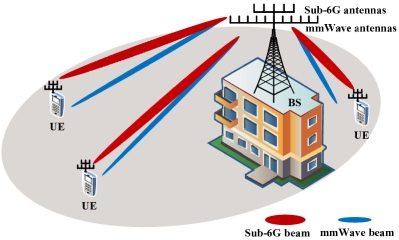
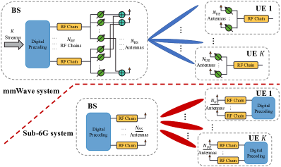
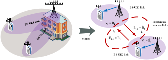
As depicted in Fig. 1a, we consider a dual-band system comprising one BS and $K$ UEs. Both the BS and UEs are assumed to employ two transceivers similar to [18, 19, 25]: one works at sub-6G frequency, and the other operates at mmWave frequency. Specifically, in the mmWave system, the BS adopts a hybrid beamforming architecture, where each of the $N_{\text{BS}}$ mmWave antennas is connected to $N_{\text{RF}}$ RF chains. Each UE adopts an analog beamforming architecture, where $N_{\text{UE}}$ mmWave antennas are fully connected with one RF chain. As for the sub-6G system, both the BS and UEs adopt the fully digital beamforming architecture and are equipped with $\underline{N_{\text{BS}}}$ and $\underline{N_{\text{UE}}}$ antennas, respectively. These beamforming architectures are illustrated in Fig. 1b.

II-A Channel Model and mmWave Downlink Communication

Due to the limited diffraction ability of mmWave signals, we adopt a geometric mmWave channel model that consists of $C$ clusters, and each cluster contributes $L$ paths. Let $\theta_{c,l}$, $\phi_{c,l}$ and $\alpha_{c,l}$ denote the angle of departure (AoD), angle of arrival (AoA), and complex gain of the $l$-th path in the $c$-th cluster, respectively. Then, the mmWave channel coefficients of the $u$-th UE, represented by $\mathbf{H}_{u}$, can be given by

$$\mathbf{H}_{u}=\sqrt{N_{\text{BS}}N_{\text{UE}}}\sum_{c=1}^{C}\sum_{l=1}^{L}\alpha_{c,l}\mathbf{a}_{\text{UE}}(\phi_{c,l})\mathbf{a}_{\text{BS}}^{H}(\theta_{c,l}),$$ (1)

where

$$\mathbf{a}_{\text{BS}}(\theta_{c,l})=\frac{1}{\sqrt{N_{BS}}}[1,e^{j\pi\sin(\theta_{c,l})},\dots,e^{j\pi(N_{BS}-1)\sin(\theta_{c,l})}]^{T},$$

$$\mathbf{a}_{\text{UE}}(\phi_{c,l})=\frac{1}{\sqrt{N_{UE}}}[1,e^{j\pi\sin(\phi_{c,l})},\dots,e^{j\pi(N_{UE}-1)\sin(\phi_{c,l})}]^{T},$$

are the steering vectors corresponding to the AoD $\theta_{c,l}$ and AoA $\phi_{c,l}$, respectively.

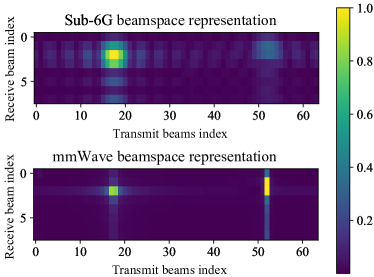
As for the sub-6G channel $\underline{{\mathbf{H}}_{u}}$, a similar geometric channel model with limited clusters is adopted. As depicted in Fig. 2, the dominant paths of the sub-6G and mmWave channels partially overlap in the angular domain, however, their total number of clusters/paths, channel gain of each path and other parameters are different [18]. In the numerical simulations later, we adopt the DeepMIMO dataset [31, 32] for network training, which is generated by running ray-tracing in sub-6G and mmWave frequencies.

Figure 2: Normalized beamspace representation of sub-6G channel and mmWave channel.

For mmWave downlink communication, denote the transmit signal vector of at the BS by $\mathbf{s}\triangleq[s_{1},\dots,s_{K}]^{T}$, where $s_{u}$ is the transmit signal to the $u$-th UE. After transmit precoding, channel propagation and receive combining, the received signal at the $u$-th UE, represented by $y_{u}$, is given by

$$y_{u}=\mathbf{v}_{u}^{H}\mathbf{H}_{u}\mathbf{F}_{\text{RF}}\sum_{i=1}^{K}{\mathbf{F}_{\text{BB}}}{[:,i]}s_{i}+\mathbf{v}_{u}^{H}\mathbf{n}_{u},$$ (2)

where $\mathbb{E}[\mathbf{s}\mathbf{s}^{H}]=\frac{P_{\text{t}}}{K}\mathbf{I}_{K}$ and $P_{\text{t}}$ denotes the total transmit power of the BS, $\mathbf{n}_{u}\in\mathcal{C}\mathcal{N}(0,\sigma_{n}^{2}\mathbf{I}_{N_{\text{UE}}})$ is the noise vector of the $u$-th UE with $\sigma_{n}^{2}$ being the noise power, $\mathbf{F}_{\text{RF}}\in\mathbb{C}^{N_{\text{BS}}\times N_{\text{RF}}}$ and $\mathbf{F}_{\text{BB}}\in\mathbb{C}^{N_{\text{RF}}\times N_{\text{RF}}}$ denote the analog beamforming matrix and digital beamforming matrix at the BS, respectively, and satisfy the power constraint $\left\lVert\mathbf{F}_{\text{RF}}\mathbf{F}_{\text{BB}}\right\rVert_{\ell_{2}}^{2}=K$, ${\mathbf{v}}_{u}\in{\mathbb{C}}^{N_{\text{UE}}\times 1}$ denotes the receive combiner of the $u$-th UE. Specially, ${\mathbf{v}}_{u}$ and each column of the analog beamforming matrix ${\mathbf{F}}_{\text{RF}}$ are selected from predefined DFT codebooks ${\mathbf{Z}}\in\mathbb{C}^{N_{\text{UE}}\times N_{\mathbf{Z}}}\triangleq[{\mathbf{z}}_{1},\dots,{\mathbf{z}}_{N_{\text{Z}}}]$ and ${\mathbf{W}}\in\mathbb{C}^{N_{\text{BS}}\times N_{\mathbf{W}}}\triangleq[{\mathbf{w}}_{1},\dots,{\mathbf{w}}_{N_{\text{W}}}]$, respectively, where $N_{\mathbf{Z}}$ and $N_{\mathbf{W}}$ denote the corresponding numbers of codewords. Without loss of generality, we assume $N_{\mathbf{Z}}=N_{\text{UE}}$ and $N_{\mathbf{W}}=N_{\text{BS}}$. Furthermore, we define ${\mathbf{h}}_{u,\text{eff}}^{H}=\mathbf{v}_{u}^{H}\mathbf{H}_{u}\mathbf{F}_{\text{RF}}\in\mathbb{C}^{1\times N_{\text{RF}}}$ as the effective channel between the $u$-th UE and BS. Accordingly, the received signal model in (2) can be rewritten as

$$y_{u}={\mathbf{h}}_{u,\text{eff}}^{H}\sum_{i=1}^{K}{\mathbf{F}_{\text{BB}}}{[:,i]}s_{i}+\mathbf{v}_{u}^{H}\mathbf{n}_{u},$$ (3)

As a result, the signal-to-interference-plus-noise ratio (SINR) of $y_{u}$, represented by $\gamma_{u}$, can be written as follows:

$$\gamma_{u}=\frac{\left\lvert\mathbf{h}_{u,\text{eff}}^{H}{\mathbf{F}_{\text{BB}}}{[:,u]}s_{u}\right\rvert^{2}}{\sum_{i\neq u}\left\lvert\mathbf{h}_{u,\text{eff}}^{H}{\mathbf{F}_{\text{BB}}}{[:,i]}s_{i}\right\rvert^{2}+\sigma_{n}^{2}\left\lVert\mathbf{v}_{u}\right\rVert^{2}_{\ell_{2}}}.$$ (4)

Given $\gamma_{u}$, the spectrum efficiency of the $u$-th UE, denoted by $R_{u}$, is given by

$$R_{u}=\log_{2}(1+\gamma_{u}).$$ (5)

Then, the overall spectrum efficiency of the considered dual-band mmWave communication system, represented by $R_{\rm{sum}}$, is

$$R_{\rm{sum}}=\sum_{u=1}^{K}R_{u}.$$ (6)

II-B Problem formulation

Our goal is to optimize the hybrid beamforming matrices at the BS $\{\mathbf{F}_{\text{BB}},\mathbf{F}_{\text{RF}}\}$ as well as the analog combiners at all the UEs $\{{\mathbf{v}}_{1},\dots,{\mathbf{v}}_{K}\}$ to maximize the sum spectrum efficiency $R_{\text{sum}}$ for the system considered. Mathematically, the following problem is considered:

$$\max_{\mathbf{F}_{\text{BB}},\mathbf{F}_{\text{RF}},\{{\mathbf{v}}_{1},\dots,{\mathbf{v}}_{K}\}} ~{}R_{\rm{sum}},$$ (7)

s.t $$~{}\mathbf{v}_{i}\in{\mathcal{Z}},\forall i\in\{1,\dots,K\},$$ (7a)

$$~{}{\mathbf{F}_{\text{RF}}}[:,j]\in{\mathcal{W}},\forall j\in\{1,\dots,N_{\text{RF}}\},$$ (7b)

$$\left\lVert\mathbf{F}_{\text{RF}}\mathbf{F}_{\text{BB}}\right\rVert_{\ell_{2}}^{2}=K.,$$ (7c)

where ${\mathcal{Z}}\triangleq\{{\mathbf{z}}_{1},\dots,{\mathbf{z}}_{N_{\text{Z}}}\}$ and ${\mathcal{W}}\triangleq\{{\mathbf{w}}_{1},\dots,{\mathbf{w}}_{N_{\text{W}}}\}$.

Traditionally, based on perfect mmWave CSI, a variety of optimization-based algorithms [9, 10] have been proposed to solve problem (7). However, the acquisition of accurate mmWave CSI requires a substantial number of pilots owing to the large number of antennas, even when using compressed sensing based algorithms [2, 33]. Furthermore, some decoupled hybrid beamforming methods have been developed for mmWave systems with limited feedback [7, 5], but these methods require extensive beam training, particularly when the number of UEs is large.

Fortunately, in the dual-band system considered, the correlation between sub-6G and mmWave frequencies have been widely investigated and demonstrated in numerous works [11, 12]. This correlation arises due to the presence of shared scatterers in the propagation environment, and thus the sub-6G channel and mmWave channel exhibit significant similarity in both time and spatial domains. Capitalizing on the spatial congruence between sub-6G and mmWave frequencies presents a promising avenue to reduce the pilot signal overhead. Motivated by these insights, our objective is to incorporate sub-6G channel information to support mmWave hybrid beamforming. Additionally, we take a pragmatic approach by considering the imperfect sub-6G channel estimate in the design.

In particular, to estimate the sub-6G channels, each UE transmits uplink training pilot sequences to the BS. Let $\underline{L_{\text{p}}}$ denote the training sequence length, and $\underline{{\mathbf{S}}_{\text{u,p}}}\in{\mathbb{C}}^{\underline{N_{\text{UE}}}\times\underline{L_{\text{p}}}}$ denote a pilot matrix with each row corresponding to a pilot sequence sent from a particular antenna of the $u$-th UE. Then, the received training signals at the BS is given by

$$\underline{{\mathbf{Y}}_{\text{p}}}=\sum\limits_{u=1}^{K}\underline{{\mathbf{H}}_{u}}^{T}\underline{{\mathbf{S}}_{\text{u,p}}}+\underline{{\mathbf{N}}_{\text{p}}},$$ (8)

where $\underline{{\mathbf{N}}_{\text{p}}}\sim{\mathcal{CN}}(0,\underline{\sigma_{n}^{2}})$ is the noise matrix with independent and identically distributed (i.i.d.) noise elements, and $\underline{\sigma_{n}^{2}}$ denotes the noise power during pilot transmission. In general, we should have $\underline{L_{\text{p}}}\geqslant K\underline{N_{\text{UE}}}$, to ensure the orthogonality between any two pilot sequences sent from different antennas of each user and from different users. Here, we simply assume that $\underline{L_{\text{p}}}=K\underline{N_{\text{UE}}}$. With this assumption and defining $\underline{{\mathbf{S}}_{\text{p}}}=[\underline{{\mathbf{S}}_{\text{1,p}}}^{T},\dots,\underline{{\mathbf{S}}_{\text{K,p}}}^{T}]^{T}\in{\mathbb{C}}^{{K\underline{N_{\text{UE}}}}\times\underline{L_{\text{p}}}}$, we can rewrite (9) as

$$\underline{{\mathbf{Y}}_{\text{p}}}=[\underline{\widehat{\mathbf{H}}_{1}}^{T},\dots,\underline{\widehat{\mathbf{H}}_{K}}^{T}]\underline{{\mathbf{S}}_{\text{p}}}+\underline{{\mathbf{N}}_{\text{p}}},$$ (9)

where $\underline{{\mathbf{S}}_{\text{p}}}$ satisfies $\underline{{\mathbf{S}}_{\text{p}}}^{H}\underline{{\mathbf{S}}_{\text{p}}}=\sqrt{\underline{P_{\text{s}}}}{\mathbf{I}}_{\underline{L_{\text{p}}}}$ with $\underline{P_{\text{s}}}$ denoting the sub-6G pilot signal power. Subsequently, the sub-6G channels can be obtained by resorting to the low-complexity least square estimation as

$$[\underline{\widehat{\mathbf{H}}_{1}}^{T},\dots,\underline{\widehat{\mathbf{H}}_{K}}^{T}]=\underline{{\mathbf{Y}}_{u,\text{p}}}~{}\underline{{\mathbf{S}}_{\text{p}}}^{-1},$$ (10)

In the subsequent sections, we shall focus on developing a framework to leverage such sub-6G channel estimate to facilitate mmWave hybrid beamforming.

III Sub-6G Information Aided Multi-User Hybrid Beamforming: Overall Design

In this section, we first discuss the key issues of utilizing sub-6G information for mmWave hybrid beamforming and then present the overall design of the proposed SA-MUHBF framework.

To effectively integrate the sub-6G channel estimates into mmWave hybrid beamforming, two main issues arise: (1) identifying the relevant sub-6G channel information for mmWave beamforming, and (2) designing an efficient hybrid beamforming scheme based on the sub-6G channel information.

To address the first issue, we need to analyze the spatial congruence between sub-6G and mmWave channels. As illustrated in Fig. 2, although there is a discrepancy in the number of paths between sub-6G and mmWave channels, their dominant path angles exhibit a strong correlation, and the normalized gains of these paths are similar. Consequently, although directly reconstructing the complete mmWave channel from sub-6G channel information is challenging, it remains possible to predict its beamspace representation by capturing the key angular and path gain features.

To tackle the second issue, decoupling the optimization of analog and digital beamforming might be an effective solution. This is because the extracted beamspace information is more useful for analog beam selection at each user, to perform user separation in the spatial domain. While digital beamforming might be more reliably designed if additional limited in-band measurements could be obtained.

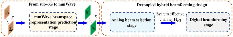
In light of the above discussions, we propose to construct the SA-MUHBF framework via three stages (illustrated in Fig. 3), as follows:

Figure 3: The overall design of SA-MUHBF framework.

• mmWave beamspace representation prediction stage: Extract the spatial information from sub-6G channel estimates and then predict mmWave beamspace representations;

• Analog beam selection stage: Select the proper analog beams based on the predicted mmWave beamspace representations while accounting for inter-user interference coordination;

• Digital beamforming stage: Obtain an effective multi-user channel ${\mathbf{H}}_{\text{eff}}$ in the digital domain after applying the analog beams selected from the previous stage, and then design an optimized digital beamforming based on ${\mathbf{H}}_{\text{eff}}$.

IV Sub-6G Information-Aided Multi-User Hybrid Beamforming: Deep-Learning Assisted Implementation

We now proceed to present a deep-learning assisted implementation of the SA-MUHBF framework. We first provide the detailed description of each stage, and then present the training procedure for the overall design.

IV-A mmWave Beamspace Representation Prediction Stage

Figure 4: An illustration of the mmWave beamspace representation prediction stage.

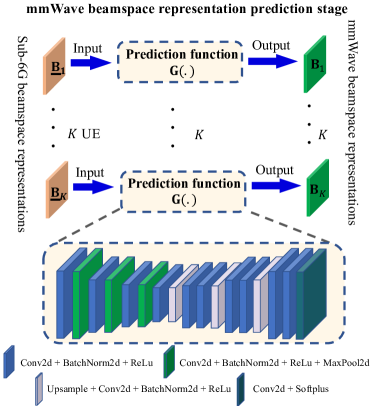
This stage is aimed at extracting the mmWave spatial information from the sub-6G channel and then predicting the mmWave beamspace representation. Taking the $u$-th UE as an example, to facilitate this extraction, we first convert the sub-6G channel estimate $\underline{\widehat{\mathbf{H}}_{u}}$ into a sub-6G beamspace representation $\underline{\widehat{\mathbf{B}}_{u}}$. This conversion is achieved by utilizing two oversampled DFT codebooks, denoted by $\underline{\mathbf{Z}}\in{\mathbb{C}}^{\underline{N_{\text{UE}}}\times N_{\text{Z}}}$ and $\underline{\mathbf{W}}\in{\mathbb{C}}^{\underline{N_{\text{BS}}}\times N_{\text{W}}}$, and the resultant $\underline{\widehat{\mathbf{B}}_{u}}$ is given by

$$\underline{\widehat{\mathbf{B}}_{u}}={|\underline{\mathbf{Z}}^{H}\underline{\widehat{\mathbf{H}}_{u}}~{}\underline{\mathbf{W}}|}.$$ (11)

Note that each element of $\underline{\widehat{\mathbf{B}}_{u}}$ indicates the likelihood of a strong path’s presence in the corresponding beamspace bin.

Subsequently, a prediction function, represented by ${\mathbf{G}}(\cdot)$, is designed to map $\underline{\widehat{\mathbf{B}}_{u}}$ into a beamspace representation of the mmWave channel, i.e.,

$$\widehat{\mathbf{B}}_{u}={\mathbf{G}}(\underline{\widehat{\mathbf{B}}_{u}}).$$ (12)

Note that the predicted $\widehat{\mathbf{B}}_{u}\in{\mathbb{R}}_{+}^{N_{\text{Z}}\times N_{\text{W}}}$ is expected to match well with the true mmWave beamspace representation ${\mathbf{B}}_{u}$, which satisfies ${\mathbf{B}}_{u}={|{\mathbf{Z}}^{H}{\mathbf{H}}_{u}{\mathbf{W}}|}$.

Towards this end and motivated by the recent success of CNNs in featrue learning, generative and reconstruction tasks [34], we propose to construct ${\mathbf{G}}(\cdot)$ based on 2D CNNs. As illustrated in Fig. 4, we adopt a stack structure of 2D CNN blocks, each of which consists of Conv2d, BatchNorm2d, ReLu, MaxPool2d and Upsample layers. Specifically, the input $\widehat{\mathbf{B}}_{u}$ is first compressed via a group of 2D CNN blocks to generate essential features, which are then used to predict the mmWave beamspace representation through a second group of 2D CNN blocks. Moreover, to ensure that each element in the output $\widehat{\mathbf{B}}_{u}$ is nonnegative, a Softplus activation function, i.e., $\text{Softplus}(x)=\log(1+e^{x})$, is adopted in the end.

IV-B Analog Beam Selection Stage

Figure 5: Illustration of the interference graph.

Given the predicted mmWave beamspace representations $\{\widehat{\mathbf{B}}_{1},\dots,\widehat{\mathbf{B}}_{K}\}$, this stage aims to perform analog beam selection for the BS and all UEs by assuming that ${\mathbf{F}}_{\text{BB}}={\mathbf{I}}_{K}$. Mathematically, we introduce a $N_{\text{Z}}\times N_{\text{W}}$ binary matrix $\tilde{\mathbf{L}}_{u}$ to represent the beam selection strategy for the $u$-th BS-UE pair, where $\|\tilde{\mathbf{L}}_{u}\|_{\ell_{0}}=1$, and $\tilde{\mathbf{L}}_{u}[i,j]=1$ indicates that the $u$-th BS-UE link adopts ${\mathbf{z}}_{i}$ and ${\mathbf{w}}_{j}$ as the combiner and analog precoder, respectively. Then, we will design an efficient mapping function from $\{\widehat{\mathbf{B}}_{1},\dots,\widehat{\mathbf{B}}_{K}\}$ to $\{\tilde{\mathbf{L}}_{1},\dots,\tilde{\mathbf{L}}_{K}\}$.

To cope with the multi-user interference, we propose a novel GNN-aided analog beam selection method. In particular, we first construct a low-complexity interference graph based on $\{\widehat{\mathbf{B}}_{1},\dots,\widehat{\mathbf{B}}_{K}\}$. Then, we design a multi-layer GNN based beam selection model where a novel graph convolution layer is proposed to update the beam selection strategies under by taking interference coordination into consideration.

IV-B1 Graph Modeling of the Multi-User mmWave System

Denote the interference graph by ${\mathcal{G}}({\mathcal{V}},{\mathcal{E}})$, where ${\mathcal{V}}$ and ${\mathcal{E}}$ represent the vertex set and edge set, respectively. In ${\mathcal{G}}({\mathcal{V}},{\mathcal{E}})$, the $u$-th vertex is used to model the $u$-th BS-UE link, and the attribute of the $u$-th vertex, represented by ${\mathbf{V}}_{u}$, is defined as the effective channel strength of the $u$-th BS-UE link. Additionally, the directed edge $(u,v)$ denotes the interference from the $u$-th link to the $v$-th link, and the attribute of the edge $(u,v)$, represented by ${\mathbf{E}}_{u,v}$, is defined as the effective interference channel strength from the $u$-th link to the $v$-th link. In the considered multi-user system, due to the absence of perfect mmWave channel knowledge, we propose to construct ${\mathcal{G}}$ based on the obtained mmWave beamspace representation estimates $\{\widehat{\mathbf{B}}_{1},\dots,\widehat{\mathbf{B}}_{K}\}$. Taking the $u$-th vertex as an example, we set ${\mathbf{V}}_{u}=\widehat{\mathbf{B}}_{u}$ and ${\mathbf{E}}_{u,v}=\widehat{\mathbf{B}}_{v}$. The resultant interference graph is shown in the right of Fig. 5. Moreover, due that the attribute of edge $(u,v)$ coincides with the attribute of the $v$-th vertex, i.e., ${\mathbf{E}}_{u,v}={\mathbf{V}}_{v}=\widehat{\mathbf{B}}_{v}$, we can only store the vertex attribute when representing the graph in the processing.

IV-B2 Multi-layer GNN Based Beam Selection Model

With the constructed interference graph ${\mathcal{G}}$, we now propose a multi-layer GNN based beam selection model, represented by ${\mathbf{S}}(\cdot)$, to produce the analog beam selection strategies of all the BS-UE links. Specifically, ${\mathbf{S}}(\cdot)$ is constructed by cascading $T$ graph convolution layers, as illustrated in Fig. 6. The inputs of each layer include the interference graph ${\mathcal{G}}$ and a set of beam selection probability matrices generated from the previous layer. Let ${\mathbf{s}}_{t}(\cdot)$ denote the $t$-th layer, and let ${\mathbf{L}}_{u}^{t}$ represent the beam selection probability matrix for the $u$-th BS-UE pair that satisfies $\|{\mathbf{L}}^{t}_{u}\|_{\ell_{1}}=1$. Then, we have

$$\{{\mathbf{L}}_{1}^{t},\dots,{\mathbf{L}}_{K}^{t}\}={\mathbf{s}}_{t}(\{{\mathbf{L}}_{1}^{t-1},\dots,{\mathbf{L}}_{K}^{t-1}\},{\mathcal{G}}).$$ (13)

Note that when $t=1$, ${\mathbf{L}}_{0}^{t}$ is initialized by a normalized version of $\widehat{\mathbf{B}}_{u}$ from the beamspace prediction stage, i.e.,

$${\mathbf{L}}_{u}^{0}=\frac{\widehat{\mathbf{B}}_{u}}{\|\widehat{\mathbf{B}}_{u}\|_{\ell_{1}}},~{}\forall~{}u\in\{1,\dots,K\}.$$ (14)

After the processing of $T$ graph convolution layers (or equivalently $T$ iterations), the produced beam selection probability matrix ${\mathbf{L}}_{u}^{T}$ is further mapped into a binary matrix $\tilde{{\mathbf{L}}}_{u}$ according to the following rule:

$$\tilde{\mathbf{L}}_{u}[i,j]=\begin{cases}1,~{}i=i_{u}^{\star},~{}j=j_{u}^{\star},\\ 0,~{}\text{otherwise}\end{cases},~{}\forall u\in\{1,\dots,K\},$$ (15)

where $(i_{u}^{\star},j_{u}^{\star})=\arg\max_{i,j}{\mathbf{L}}_{u}^{T}[i,j]$ contains the row and column indices correspond to the largest element in $\tilde{\mathbf{L}}_{u}$. Then, the analog beamforming vectors for the $u$-th BS-UE link are set as

$${\mathbf{F}}_{\text{RF}}[:,u]={\mathbf{w}}_{j_{u}^{\star}},~{}{\mathbf{v}}_{u}={\mathbf{z}}_{i_{u}^{\star}},~{}\forall~{}u\in\{1,\dots,K\}.$$ (16)

Next, we present the architecture of the graph convolution layer in details.

IV-B3 Architecture of the Graph Convolution Layer

Figure 6: Illustration of our proposed multi-layer GNN model.

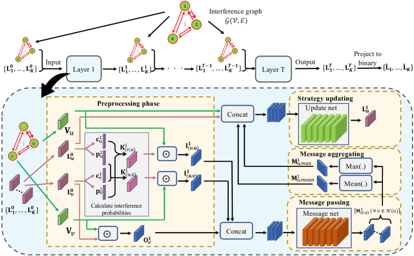
Aiming to improve the analog beam selection quality, we propose a novel graph convolution layer, which incorporates a preprocessing phase for the inputs and a 2D CNN based graph convolution for the preprocessed features, as illustrated in Fig. 6. In the preprocessing phase, both the effective signal strength and interference strength among different BS-UE links are explicitly modeled. Specifically, taking the $t$-th layer as an example, we first calculate the probabilities of different analog combiners at the UEs and different analog beamformers at the BS, represented by $\{{\mathbf{c}}_{1}^{t},\dots,{\mathbf{c}}_{K}^{t}\}$ and $\{{\mathbf{p}}_{1}^{t},\dots,{\mathbf{p}}_{K}^{t}\}$, respectively, by taking $\{{\mathbf{L}}^{t-1}_{1},\dots,{\mathbf{L}}^{t-1}_{K}\}$ and ${\mathcal{G}}$ as inputs, i.e.,

$${\mathbf{c}}_{u}^{t}[i] =\sum_{j=1}^{N_{\mathbf{Z}}}{\mathbf{L}}_{u}^{t}[i,j],~{}\forall~{}i\in\{1,\dots,N_{\mathbf{Z}}\},~{}\forall~{}u\in\{1,\dots,K\},$$

$${\mathbf{p}}_{u}^{t}[j] =\sum_{i=1}^{N_{\mathbf{W}}}{\mathbf{L}}_{u}^{t}[i,j],~{}\forall~{}j\in\{1,\dots,N_{\mathbf{W}}\},~{}\forall~{}u\in\{1,\dots,K\},$$

where ${\mathbf{c}}_{u}^{t}[i]$ and ${\mathbf{p}}_{u}^{t}[j]$ represent the probabilities of the $u$-th link selecting ${\mathbf{z}}_{i}$ and ${\mathbf{w}}_{j}$ as the combiner and analog beamformer, respectively. Subsequently, with $\{{\mathbf{c}}_{1}^{t},\dots,{\mathbf{c}}_{K}^{t}\}$ and $\{{\mathbf{p}}_{1}^{t},\dots,{\mathbf{p}}_{K}^{t}\}$, we obtain the interference probabilities among different links, represented by ${\mathbf{K}}_{(u,v)}^{t}$, as follows:

$${\mathbf{K}}_{(u,v)}^{t}={\mathbf{c}}_{v}^{t}{{\mathbf{p}}_{u}^{t}}^{T},~{}\forall~{}u,~{}v\in\{1,\dots,K\},~{}u\neq v,$$ (17)

where ${\mathbf{K}}_{(u,v)}^{t}\in{\mathbb{R}}_{+}^{N_{\text{Z}}\times N_{\text{W}}}$ and $\|{\mathbf{K}}_{(u,v)}^{t}\|_{\ell_{1}}=1$. Then, ${\mathbf{K}}_{(u,v)}^{t}$ is further converted to a matrix ${\mathbf{I}}^{t}(u,v)\in{\mathbb{R}}_{+}^{N_{\text{Z}}\times N_{\text{W}}}$ to capture the potential interference strength of the $u$-th link to the $v$-th link, via

$${\mathbf{I}}_{(u,v)}^{t}={\mathbf{K}}_{(u,v)}^{t}\odot{\mathbf{V}}_{v},~{}\forall~{}u,~{}v\in\{1,\dots,K\},~{}u\neq v.$$ (18)

Additionally, the potential effective signal strength of the $u$-th BS-UE link, denoted by ${\mathbf{O}}_{u}^{t}\in{\mathbb{R}}_{+}^{N_{\text{Z}}\times N_{\text{W}}}$ can be obtained as

$${\mathbf{O}}_{u}^{t}={\mathbf{L}}_{u}^{t-1}\odot{\mathbf{V}}_{u},~{}\forall~{}u\in\{1,\dots,K\}.$$ (19)

The above preprocessing effectively fuses the predicted beamspace representation and beam selection probabilities generated from the previous graph convolution layer.

Next, the obtained 2D matrices $\{{\mathbf{O}}_{u}^{t}|\forall u\in\{1,\dots,K\}\}$ and $\{{\mathbf{I}}_{(u,v)}^{t}|~{}\forall~{}u,~{}v\in\{1,\dots,K\},~{}u\neq v\}$ are further processed by graph convolution, which involves three phases, i.e., message passing, message aggregation and strategy updating.

Message Passing Phase

Specifically, taking the $u$-th vertex and its neighboring vertex $v$ as an example, we employ a 2D CNN structure, denoted by $\text{CNN1}(\cdot)$, to extract features from the mutual potential interference strength $\{{\mathbf{I}}_{(u,v)}^{t},{\mathbf{I}}_{(v,u)}^{t}\}$ and the effective signal strength of the $u$-th link ${\mathbf{O}}_{u}^{t}$ as the message. In particular, the message from the $u$-th vertex to the $v$-th vertex is denoted by ${\mathbf{M}}_{(u,v)}^{t}\in{\mathbb{R}}_{+}^{N_{\text{Z}}\times N_{\text{W}}}$ and is calculated as

$${\mathbf{M}}_{(u,v)}^{t}=\text{CNN1}\left(\text{CONCAT}({\mathbf{O}}_{u}^{t},{\mathbf{I}}_{(u,v)}^{t},{\mathbf{I}}_{(v,u)}^{t})\right),$$ (20)

where $\text{CONCAT}(\cdot)$ concatenates the input matrices in the $0$-th dimension. Each vertex adopts the same operation as in (20) to produce its messages and subsequently sends them to its neighboring vertices along the directed edges.

Message Aggregating Phase

In this phase, each vertex conducts message aggregation over its received messages. For instance, denoting the received messages of the $u$-th vertex by $\{{\mathbf{M}}_{(u,v)}~{}|~{}\forall~{}v\in{\mathcal{N}}(u)\}$, then the message aggregation is implemented through

$${\mathbf{M}}_{u,\text{max}}^{t} =\text{MAX}(\{{\mathbf{M}}_{(v,u)}^{t}~{}|~{}\forall~{}v\in{\mathcal{N}}(u)\}),$$

$${\mathbf{M}}_{u,\text{mean}}^{t} =\text{MEAN}(\{{\mathbf{M}}_{(v,u)}^{t}~{}|~{}\forall~{}v\in{\mathcal{N}}(u)\}),$$ (21)

where $\text{MAX}(\cdot)$ selects the maximum value of the input matrices in an element-wise manner, i.e.,

$${\mathbf{M}}_{u,\text{max}}^{t}[i,j]=\max\left(\{{\mathbf{M}}_{(v,u)}^{t}[i,j]~{}|~{}\forall~{}v\in{\mathcal{N}}(u)\}\right),$$

$$\forall~{}i\in\{1,\dots,N_{\mathbf{Z}}\},\forall~{}j\in\{1,\dots,N_{\mathbf{W}}\}.$$ (22)

Similarly, the operation $\text{MEAN}(\cdot)$ returns the mean value of the input matrices in an element-wise manner, i.e.,

$${\mathbf{M}}_{u,\text{mean}}^{t}[i,j]=\frac{1}{\text{card}({\mathcal{N}}(u))}\sum\limits_{v\in{\mathcal{N}}(u)}{\mathbf{M}}_{(v,u)}^{t}[i,j],$$

$$\forall~{}i\in\{1,\dots,N_{\mathbf{Z}}\},\forall~{}j\in\{1,\dots,N_{\mathbf{W}}\}.$$ (23)

Strategy Updating Phase

With ${\mathbf{M}}_{u,\text{max}}^{t}$, ${\mathbf{M}}_{u,\text{mean}}^{t}$, ${\mathbf{L}}_{u}^{t-1}$, and ${\mathbf{V}}_{u}$, we employ a 2D CNN structure again to combine them and then produce the updated beam pair selection probability ${\mathbf{L}}_{u}^{t}$ as

$${\mathbf{L}}_{u}^{t}=\text{CNN2}\left(\text{CONCAT}({\mathbf{M}}_{u,\text{max}}^{t},{\mathbf{M}}_{u,\text{mean}}^{t},{\mathbf{L}}_{u}^{t-1},{\mathbf{V}}_{u})\right).$$

Overall, it can be seen that the proposed analog beam selection network design follows the “learning and optimization” paradigm [26], i.e., we construct neural networks by cascading several learnable layers to iterative refine the beam selection strategy. An efficient preprocessing phase within ${\mathbf{S}}(\cdot)$ is introduced to capture the effective signal and interference strengths by integrating the beamspace representation and beam selection strategy. Such customized design is different from several state-of-the-art GNNs, such as the TransformerConv GNN [35] and the GNN in GBLinks [29], which do not preprocess the inputs and utilize either 1D CNNs or MLPs for graph convolution. Therefore, ${\mathbf{S}}(\cdot)$ is envisioned to exhibit superior interpretability and more robust performance, as will be validated in Section V.

IV-C Digital Beamforming Stage

Upon obtaining the analog beamforming vectors at BS and UEs from the previous stage, the digital beamforming vectors at the BS are then optimized in this stage. To this end, we propose to first estimate the effective BS-UE channel ${\mathbf{H}}_{\text{eff}}$ in the digital domain with given analog beams and then optimize the digital beamforming vectors based on the estimated $\widehat{\mathbf{H}}_{\text{eff}}$.

Specifically, to obtain $\widehat{\mathbf{H}}_{\text{eff}}$, each UE transmits uplink training pilot sequences to the BS. Let $L_{\text{p}}$ represent the training pilot sequence length, and let ${\mathbf{s}}_{\text{u,p}}^{T}\in{\mathbb{C}}^{1\times L_{\text{p}}}$ denote the pilot vector of the $u$-th UE. Then, the received training signals at the BS is given by

$${\mathbf{Y}}_{\text{p}} =\sum\limits_{u=1}^{K}{\mathbf{F}}_{\text{RF}}^{T}{\mathbf{H}}_{u}^{T}{\mathbf{v}}_{u}^{*}{\mathbf{s}}_{\text{u,p}}^{T}+{\mathbf{F}}_{\text{RF}}^{T}{\mathbf{N}}_{\text{p}},$$

$$=\sum\limits_{u=1}^{K}{\mathbf{h}}_{\text{u,eff}}{\mathbf{s}}_{\text{u,p}}^{T}+{\mathbf{F}}_{\text{RF}}^{T}{\mathbf{N}}_{\text{p}},$$ (24)

where ${\mathbf{N}}_{\text{p}}\sim\mathcal{CN}(0,\sigma_{n}^{2})$ is the noise matrix with i.i.d. noise elements, and $\sigma_{n}^{2}$ denotes the channel noise power. In general, we should have $L_{\text{p}}\geqslant K$ to ensure the orthogonality of any two pilot sequences of different UEs, and here we assume that $L_{\text{p}}=K$. With this assumption and by defining ${\mathbf{S}}_{\text{p}}=[{\mathbf{s}}_{\text{u,p}}^{T},\dots,{\mathbf{s}}_{\text{u,p}}^{T}]^{T}\in{\mathbb{C}}^{K\times L_{\text{p}}}$, we can rewrite (24) as

$${\mathbf{Y}}_{\text{p}} =[{\mathbf{h}}_{\text{1,eff}},\dots,{\mathbf{h}}_{\text{K,eff}}]{\mathbf{S}}_{\text{p}}+{\mathbf{F}}_{\text{RF}}^{T}{\mathbf{N}}_{\text{p}},$$

$$={\mathbf{H}}_{\text{eff}}^{T}{\mathbf{S}}_{\text{p}}+{\mathbf{F}}_{\text{RF}}^{T}{\mathbf{N}}_{\text{p}},$$ (25)

where ${\mathbf{S}}_{\text{p}}$ satisfies ${\mathbf{S}}_{\text{p}}^{H}{\mathbf{S}}_{\text{p}}=P_{\text{s}}{\mathbf{I}}_{L_{\text{p}}}$, and $P_{\text{s}}$ represents the mmWave training pilot signal power. As a result, the effective channel ${\mathbf{H}}_{\text{eff}}$ can be estimated as

$$\widehat{\mathbf{H}}_{\text{eff}}=({\mathbf{Y}}_{\text{p}}{\mathbf{S}}_{\text{p}}^{-1})^{T}.$$ (26)

Based on $\widehat{\mathbf{H}}_{\text{eff}}\triangleq[\hat{\mathbf{h}}_{\text{1,eff}}^{*},\dots,\hat{\mathbf{h}}_{\text{K,eff}}^{*}]$, the LMMSE digital beamforming scheme proposed in [36] is adopted for inter-user interference coordination in the digital domain. The resultant beamformer ${\mathbf{F}}_{\text{BB}}$ is given by

$${\mathbf{F}}_{\text{BB}}=\frac{\sqrt{K}\tilde{\mathbf{F}}_{\text{BB}}}{\lVert\mathbf{F}_{\text{RF}}\tilde{\mathbf{F}}_{\text{BB}}\lVert_{\ell_{2}}},$$ (27)

where $\tilde{\mathbf{F}}_{\text{BB}}$ is computed as

$${\tilde{\mathbf{F}}_{\text{BB}}}=\widehat{\mathbf{H}}_{\text{eff}}^{H}\left(\widehat{\mathbf{H}}_{\text{eff}}\widehat{\mathbf{H}}_{\text{eff}}^{H}+\frac{K\sigma_{n}^{2}}{P_{t}}\mathbf{I}_{\text{K}}\right)^{-1}\mathbf{G},$$ (28)

with $\mathbf{G}=\text{diag}\left\{\|\hat{\mathbf{h}}_{1,\text{eff}}\|_{\ell_{2}},\dots,\|\hat{\mathbf{h}}_{K,\text{eff}}\|_{\ell_{2}}\right\}$.

IV-D Training of SA-MUHBF

To train the proposed SA-MUHBF, a two-step approach is employed, where we first train the prediction network ${\mathbf{G}}(\cdot)$, and then train the GNN ${\mathbf{S}}(\cdot)$ by freezing the parameters of ${\mathbf{G}}(\cdot)$.

IV-D1 Training of the Prediction Network ${\mathbf{G}}(\cdot)$

The training process of ${\mathbf{G}}(\cdot)$ is conducted in a supervised manner. The loss function is defined as the normalized mean square error (NMSE) between the predicted mmWave beamspace representation $\widehat{\mathbf{B}}$ and the true mmWave beamspace representation ${\mathbf{B}}$, i.e.,

$$l_{1}=\frac{\|\widehat{\mathbf{B}}-{\mathbf{B}}\|_{\ell_{2}}}{\left\lVert{\mathbf{B}}\right\lVert_{\ell_{2}}}.$$ (29)

Minimizing $l_{1}$ encourages the convergence of the predicted $\widehat{\mathbf{B}}$ towards the true ${\mathbf{B}}$.

IV-D2 Training of the Multi-Layer GNN Model ${\mathbf{S}}(\cdot)$

Once ${\mathbf{G}}(\cdot)$ is trained, we proceed to train the GNN model ${\mathbf{S}}(\cdot)$ in an unsupervised manner by fixing the parameters of ${\mathbf{G}}(\cdot)$. The goal of training ${\mathbf{S}}(\cdot)$ is to generate beam pair selection strategies $\{{\mathbf{L}}_{1},\dots,{\mathbf{L}}_{K}\}$ that maximizes the sum spectrum efficiency defined in (6). However, it is noted that the projection operation at the end of ${\mathbf{S}}(\cdot)$ is not differentiable, which prevents the back propagation in the training. To tackle this problem, we propose a novel beam selection probability based loss function. To improve the convergence of the multi-layer GNN, instead of only using the beam selection probabilities generated by the last layer, we propose to aggregate the beam selection probabilities at all the layers, i.e.,

$$\bar{\mathbf{L}}_{u}=\alpha_{1}{\mathbf{L}}_{u}^{1}+\dots+\alpha_{T}{\mathbf{L}}_{u}^{T},~{}\forall~{}u\in\{1,\dots,K\},$$ (30)

where $\alpha_{1},\dots,\alpha_{T}$ denote the combining weights that satisfy $\sum\nolimits_{t=1}^{T}\alpha_{t}=1$ and $\alpha_{1}<\dots<\alpha_{T}$. Moreover, based on $\{\bar{\mathbf{L}}_{1},\dots,\bar{\mathbf{L}}_{K}\}$, we can obtain the aggregated interference probability, represented by $\{\bar{\mathbf{K}}_{(u,v)}|~{}\forall~{}u,~{}v\in\{1,\dots,K\},~{}u\neq v\}$, as follows:

$$\bar{\mathbf{K}}_{(u,v)}=\bar{\mathbf{c}}_{v}{\bar{\mathbf{p}}_{u}}^{T},~{}\forall~{}u,~{}v\in\{1,\dots,K\},~{}u\neq v,$$

$$\bar{\mathbf{c}}_{v}[i]=\sum_{j=1}^{N_{\mathbf{Z}}}\bar{\mathbf{L}}_{v}[i,j],\forall i\in\{1,\dots,N_{\mathbf{Z}}\},\forall v\in\{1,\dots,K\},$$

$$\bar{\mathbf{p}}_{u}[j]=\sum_{i=1}^{N_{\mathbf{W}}}\bar{\mathbf{L}}_{u}[i,j],\forall j\in\{1,\dots,N_{\mathbf{W}}\},\forall u\in\{1,\dots,K\}.$$

In this way, we can construct a surrogate function of the original spectrum efficiency in (6) as

$$\bar{R}_{u}=\log_{2}\left(\frac{\sum\limits_{i=1}^{N_{\text{Z}}}\sum\limits_{j=1}^{N_{\text{Z}}}\bar{\mathbf{L}}_{u}[i,j]|{\mathbf{z}}_{i}^{H}{\mathbf{H}}_{u}{\mathbf{w}}_{j}s_{u}|^{2}}{\sum\limits_{v\neq u}\sum\limits_{i=1}^{N_{\text{Z}}}\sum\limits_{j=1}^{N_{\text{W}}}\bar{\mathbf{K}}_{(v,u)}[i,j]\left\rvert{\mathbf{z}}_{i}^{H}{\mathbf{H}}_{u}{\mathbf{w}}_{j}s_{i}\right\rvert^{2}+\sigma_{n}^{2}}\right),$$

$$\forall~{}u\in\{1,\dots,K\},$$ (31)

and form the following loss function for training ${\mathbf{S}}(\cdot)$:

$$l_{2}=-\sum_{u=1}^{K}\bar{R}_{u}.$$ (32)

V Numerical Results

In this section, we conduct extensive numerical simulations to evaluate the proposed SA-MUHBF based on the DeepMIMO dataset [31, 32]. We first introduce the simulation setup and training parameters. Subsequently, we compare the performance of SA-MUHBF with various baselines, verifying its performance gain and generalization capability under various system configurations.

V-A Simulation Setup and Training Parameters

Figure 7: Top view of the “O1” scenario and the regions used in our simulation.

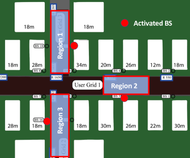
Consider the outdoor “O1” scenario of the DeepMIMO dataset, the top view of which is depicted in Fig. 7. Three regions, i.e., BS 17 (R4000-R5200), BS 3 (R750-R1300), and BS 15 (R3300-R3800), as depicted in Fig. 7, are selected for the subsequent simulation. The heights of the three activated BSs are 15m, while the UEs in these regions are at the height of 1.5m and are uniformly distributed. The relevant parameters for the dual-band system considered are provided in Table I.

TABLE I: Simulation Parameters

Notations	Parameters	Values
$f_{c}$, $\underline{f_{c}}$	Operating frequency of mmWave/sub-6G system (GHz)	28, 3.5
$W$, $\underline{W}$	Bandwidth of mmWave/sub-6G system (GHz)	0.5, 0.02
$N_{\text{BS}}$, $\underline{N_{\text{BS}}}$	Number of mmWave/sub-6G antennas at the BS	64, 16
$N_{\text{UE}}$, $\underline{N_{\text{UE}}}$	Number of mmWave/sub-6G antennas at each UE	8, 4
$P_{\text{t}}$	Total power of mmWave downlink (dBm)	40
$P_{\text{s}}$, $\underline{P_{\text{s}}}$	Power of mmWave/sub-6G pilot signals (dBm)	30, 20
$\sigma_{n}^{2}$, $\underline{\sigma_{n}^{2}}$	Noise power of mmWave/sub-6G system (dBm)	$-173.8+90+10\log_{10}(W)$ $-173.8+90+10\log_{10}(\underline{W})$

Besides, the network parameters of the beamspace representation prediction network ${\mathbf{G}}(\cdot)$ are provided in the left column of Table II. To train ${\mathbf{G}}(\cdot)$, we first collect samples from region 1. Specifically, after running ray-tracing in the sub-6G and mmWave frequencies, we obtain a total number of 200,000 samples, each of which is represented by $\{\widehat{\underline{\mathbf{H}}},{\mathbf{H}}\}$. Then, they are randomly divided into a training dataset, a validation dataset, and a testing dataset with a partition ratio of 0.4:0.1:0.5, and the batchsize $b_{\text{G}}$ is fixed at 128. The initial learning rate of ${\mathbf{G}}(\cdot)$, denoted by $\delta_{\text{G}}$, is set to $1\times 10^{-4}$, and is scheduled via the “ReduceLROnPlateau” learning rate scheduler [37], which automatically reduces the learning rate when the model’s performance on the validation set ceases to improve or demonstrates only marginal improvements over a specified number of training epochs.

As for the analog beam selection network ${\mathbf{S}}(\cdot)$, we consider a GNN model consisting of $T=3$ graph convolution layers, and the corresponding combining weights $\alpha_{1}$, $\alpha_{2}$, and $\alpha_{3}$ are set to 0.1, 0.2, and 0.7, respectively. Each layer of ${\mathbf{S}}(\cdot)$ has the same network architecture, and the detailed parameters are provided in Table II. To train ${\mathbf{S}}(\cdot)$, we first collect a total number of 24,000 multi-user samples from region 1, each of which includes the sub-6G channel estimates and mmWave channels of all the $K$ UEs, i.e., $\{\underline{\widehat{\mathbf{H}}_{1}},{\mathbf{H}}_{1},\dots,\underline{\widehat{\mathbf{H}}_{K}},{\mathbf{H}}_{K}\}$. These samples are fed into the trained ${\mathbf{G}}(\cdot)$ to generate the predicted mmWave beamspace representations as new data samples for ${\mathbf{S}}(\cdot)$, which is represented by $\{\underline{\widehat{\mathbf{B}}_{1}},{\mathbf{H}}_{1},\dots,\underline{\widehat{\mathbf{B}}_{K}},{\mathbf{H}}_{K}\}$.

The obtained data samples are further divided into a training dataset, a validation dataset, and a testing dataset with a partition ratio of 0.4:0.1:0.5, and the batchsize $b_{\text{S}}$ is also fixed at 128. The initial learning rate of ${\mathbf{S}}(\cdot)$, denoted by $\delta_{\text{S}}$, is also set to $1\times 10^{-4}$, which will be automatically adjusted through the “ReduceLROnPlateau” learning rate scheduler, similar to the training of ${\mathbf{G}}(\cdot)$.

TABLE II: Input/Output Channels of Each Block in
${\mathbf{G}}(\cdot)$, $\text{CNN1}(\cdot)$ and $\text{CNN2}(\cdot)$

${\mathbf{G}}(\cdot)$	$\text{CNN1}(\cdot)$	$\text{CNN2}(\cdot)$
(1, 64)	(3, 12)	(4, 12)
(64, 64)	(12, 24)	(12, 24)
(64, 128)	(24, 12)	(24, 12)
(128, 128)	(12, 6)	(12, 6)
(128, 256)	(6, 1)	(6, 1)
(256, 256)$\times 3$
(256, 128)
(128, 128)$\times 2$
(128, 64)
(64, 64)$\times 4$
(64, 1)

V-B Baselines

For performance comparison, we first introduce two baselines from [23] as follows:

• Uncoordinated method: This method performs mmWave analog beam selection directly based on the oversampled beamspace representation of sub-6G channel estimate $\underline{\widehat{\mathbf{B}}_{u}}={|\underline{\mathbf{Z}}^{H}\underline{\widehat{\mathbf{H}}_{u}}~{}\underline{\mathbf{W}}|}\in{\mathbb{R}}_{+}^{N_{\text{Z}}\times N_{\text{W}}}$. Specifically, supposing $(i_{u}^{\star},j_{u}^{\star})=\arg\max_{i,j}|\underline{\widehat{\mathbf{B}}_{u}}[i,j]|$, beam pair $(\mathbf{z}_{i_{u}^{\star}},\mathbf{w}_{j_{u}^{\star}})$ is then selected as the analog precoder at BS and combiner at the $u$-th UE, respectively. As for digital beamforming, LMMSE precoder is formed based on estimate of effective channel in digital domain after applying the analog beams selected for each BS-UE pair, as that in SA-MUHBF.

• Coordinated method: This method involves sequential mmWave analog beam selection directly based on the oversampled beamspace representation of sub-6G channel estimate. In each iteration, a subset of candidate mmWave beams is identified and an exhaustive search beam training is performed over such a subset to determine the best analog beam pair for the BS-UE considered. Specifically, define $b_{\text{r}}=\frac{N_{\text{UE}}}{\underline{N_{\text{UE}}}}$ and $b_{\text{c}}=\frac{N_{\text{BS}}}{\underline{N_{\text{BS}}}}$ to account for the angular resolution difference between sub-6G and mmWave channels. Then the candidate beam subset constructed for the $u$-th BS-UE pair is defined as ${\mathcal{C}}_{u}=\{(\mathbf{z}_{i},\mathbf{w}_{j})|r_{u}^{\star}\leqslant i\leqslant r_{u}^{\star}+b_{\text{r}}-1,c_{1}^{\star}\leqslant j\leqslant c_{1}^{\star}+b_{\text{c}}-1\}$ with

  $$(r_{u}^{\star},c_{u}^{\star})=\arg\max_{r,c}\frac{1}{b_{\text{r}}b_{\text{c}}}\sum\limits_{i=r}^{r+b_{\text{r}}-1}\sum\limits_{j=c}^{c+b_{\text{c}}-1}|\underline{\widehat{\mathbf{B}}_{u}}[i,j]|,$$ (33)

  where the rows $\{\underline{\widehat{\mathbf{B}}_{u}}[:,j_{1}^{\star}],\dots,\underline{\widehat{\mathbf{B}}_{u}}[:,j_{u-1}^{\star}]\}$ have been set to zeros for interference coordination purpose, once $(i_{1}^{\star},j_{1}^{\star}),\dots,(i_{u-1}^{\star},j_{u-1}^{\star})$ beam-pairs are selected for the previous $(u-1)$ BS-UE pairs. As for digital beamforming, LMMSE precoder is formed based on estimate of effective channel in digital domain as before.

In addition, we also consider the integration of mmWave beamspace prediction network ${\mathbf{G}}(\cdot)$ with the above two baselines for comparison:

• ${\mathbf{G}}(\cdot)$+uncoordinated method: This method uses ${\mathbf{G}}(\cdot)$ proposed to generate predicted mmWave beamspace representation $\widehat{\mathbf{B}}_{u}$ and then replace $\underline{\widehat{\mathbf{B}}_{u}}$ in the previous uncoordinated method with $\widehat{\mathbf{B}}_{u}$ for analog beam selection, and the other steps remain the same.

• ${\mathbf{G}}(\cdot)$+coordinated method: This method combines ${\mathbf{G}}(\cdot)$ for generating predicted mmWave beamspace representation $\widehat{\mathbf{B}}_{u}$, followed by a sequential mmWave analog beam selection process based on $\widehat{\mathbf{B}}_{u}$. Initially, the method selects the beam pair $(\mathbf{z}_{i_{1}^{\star}},\mathbf{w}_{j_{1}^{\star}})$ as the analog precoder at the BS and combiner at the first UE, respectively, where $(i_{1}^{\star},j_{1}^{\star})=\arg\max_{i,j}|\widehat{{\mathbf{B}}}_{1}[i,j]|$. For subsequent iterations with $u\geq 2$, once $(i_{1}^{\star},j_{1}^{\star}),\dots,(i_{u-1}^{\star},j_{u-1}^{\star})$ mmWave beam pairs have been selected for the previous $(u-1)$ BS-UE pairs, the rows ${{\widehat{\mathbf{B}}_{u}}[:,j_{1}^{\star}],\dots,{\widehat{\mathbf{B}}_{u}}[:,j_{u-1}^{\star}]}$ are zeroed out. Then, the beam pair with indices $(i_{u}^{\star},j_{u}^{\star})=\arg\max_{i,j}|\widehat{{\mathbf{B}}}_{u}[i,j]|$ is chosen for the $u$-th BS-UE pair. Regarding digital beamforming, LMMSE precoder is formed based on the estimate of the effective channel in the digital domain, as in previous methods.

Table III highlights the differences between the baselines and the SA-MUHBF proposed.

V-C Performance Evaluation and Comparison

TABLE III: Comparison of Different Methods

Method	mmWave beamspace prediction	Analog beam selection	Digital beamforming
Uncoordinated method	✗	uncoordinated beam selection based on sub-6G $\underline{\widehat{\mathbf{B}}}$	LMMSE precoder
Coordinated method	✗	sequential beam selection based on sub-6G $\underline{\widehat{\mathbf{B}}}$	LMMSE precoder
${\mathbf{G}}(\cdot)$+uncoordinated method	CNN-aided: ${\widehat{\mathbf{B}}}={\mathbf{G}}(\underline{\widehat{\mathbf{B}}})$	uncoordinated beam selection based on predicted mmWave ${\widehat{\mathbf{B}}}$	LMMSE precoder
${\mathbf{G}}(\cdot)$+coordinated method	CNN-aided: ${\widehat{\mathbf{B}}}={\mathbf{G}}(\underline{\widehat{\mathbf{B}}})$	sequential beam selection based on predicted mmWave ${\widehat{\mathbf{B}}}$	LMMSE precoder
Our proposed SA-MUHBF	CNN-aided: ${\widehat{\mathbf{B}}}={\mathbf{G}}(\underline{\widehat{\mathbf{B}}})$	GNN-aided: $\{\tilde{\mathbf{L}}_{1},\dots,\tilde{\mathbf{L}}_{K}\}={\mathbf{S}}(\widehat{{\mathbf{B}}}_{1}\dots,\widehat{{\mathbf{B}}}_{K})$	LMMSE precoder

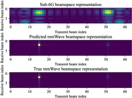
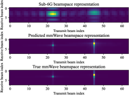
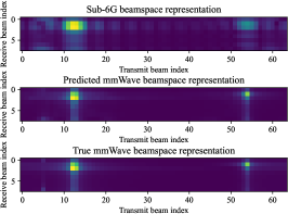
We first show the effectiveness of mmWave beamspace prediction network ${\mathbf{G}}(\cdot)$ and demonstrate the overall performance superiority of SA-MUHBF over the aforementioned baselines.

Specifically, in Fig. 8, we present the beamspace representations of the sub-6G channel estimate $\underline{\widehat{\mathbf{B}}}_{u}$, the predicted mmWave channel beamspace $\widehat{{\mathbf{B}}}_{u}$, and the actual mmWave channel beamspace ${\mathbf{B}}_{u}$ for three instances, with a sub-6G pilot signal power $\underline{P_{\text{s}}}=20~{}\text{dBm}$. It is evident that the prediction network ${\mathbf{G}}(\cdot)$ adeptly extracts spatial information from the sub-6G channel estimate, producing accurate predictions of ${\mathbf{B}}$, encompassing both the angles and gains of dominant paths. Moreover, we assess the NMSE between $\widehat{{\mathbf{B}}}_{u}$ and ${\mathbf{B}}_{u}$, as defined in (29), averaged across all samples in the testing dataset. The resulting NMSE is merely 0.0894, further substantiating the effectiveness of ${\mathbf{G}}(\cdot)$.

(a) Instance 1

(b) Instance 2

(c) Instance 3

Figure 8: Comparison between sub-6G beamspace representation $\underline{\widehat{\mathbf{B}}}_{u}$, predicted mmWave beamspace representation $\widehat{\mathbf{B}}_{u}$, and ture mmWave beamspace representation ${\mathbf{B}}_{u}$.

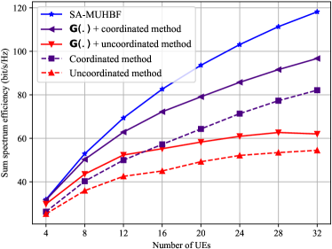
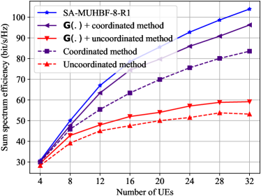
After fine-tuning ${\mathbf{G}}(\cdot)$, we next evaluate the performance of SA-MUHBF and compare against the baselines. Fig. 9 plots the sum spectrum efficiency of different methods across different number of UEs $K$. It can be seen that “${\mathbf{G}}(\cdot)$+uncoordinated method” and “${\mathbf{G}}(\cdot)$+coordinated method” outperform their respective counterparts, “uncoordinated method” and “coordinated method”. This underscores the importance of translating sub-6G channel estimates into mmWave beam space representation for effective mmWave beam selection. Moreover, our proposed SA-MUHBF consistently outperforms all baselines. Specifically, we observe performance gains of 0.5% at 4 UEs, 5.2% at 8 UEs, 14.4% at 16 UEs, and 22.2% at 32 UEs over the best-performing baseline. Notably, this improvement becomes more pronounced with increasing $K$, suggesting that the GNN-based network ${\mathbf{S}}(\cdot)$ in SA-MUHBF is highly effective in optimizing analog beam selection through learned graph convolutions, as opposed to the lack of interference coordination or heuristic interference coordination present in the baseline methods.

Figure 9: Performance comparison between SA-MUHBF and four baselines as the number of UEs increases.

(a)

(b)

Figure 10: Performance comparison as $\underline{P_{\text{s}}}$ varies, the number of UEs $K$ is fixed at 16, and the number of sub-6G antennas is fixed at $(4,16)$: (a) the prediction NMSE of ${\mathbf{G}}(\cdot)$ under different $\underline{P_{\text{s}}}$ values, (b) the sum spectrum efficiency achieved by different methods.

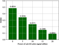
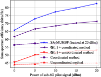
Next, we adopt the ${\mathbf{G}}(\cdot)$ and ${\mathbf{S}}(\cdot)$ models, trained with pilot signal power $\underline{P_{s}}=20~{}\text{dBm}$ as above, to assess the performance of SA-MUHBF across various $\underline{P_{\text{s}}}$ values that directly impact the quality of sub-6G channel estimate. Fig. 10a shows the NMSE of ${\mathbf{G}}(\cdot)$ versus $\underline{P_{s}}$ for SA-MUHBF, while Fig. 10b illustrates the achievable spectrum efficiency versus $\underline{P_{s}}$ under different methods with $K=16$ UEs. It is evident that SA-MUHBF consistently outperforms all considered baselines and maintains significant gain over the best-performing baseline. These results confirm the robustness of SA-MUHBF across varying qualities of sub-6G channel estimates for optimizing mmWave beamforming.

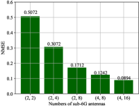
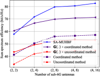
Furthermore, we investigate the performance of SA-MUHBF under various sub-6G antenna configurations $(\underline{N_{\text{r}}},\underline{N_{\text{t}}})$. It is important to note that different antenna setups impact the angular resolution of the sub-6G channel estimate and the dimension of the sub-6G beamspace representation. Hence, we train separate ${\mathbf{G}}(\cdot)$ and ${\mathbf{S}}(\cdot)$ models for each considered configuration. Fig. 11 displays the results for $(\underline{N_{\text{r}}},\underline{N_{\text{t}}})$ combinations including $(2,~{}2)$, $(2,~{}4)$, $(2,~{}8)$, $(4,~{}8)$, and $(4,~{}16)$. With small values for $\underline{N_{\text{r}}}$ or $\underline{N_{\text{t}}}$, the angular resolution in the sub-6G channel estimate is limited, making it relatively challenging to extract mmWave spatial information, as indicated by the high NMSE of ${\mathbf{G}}(\cdot)$ shown in Fig. 11a when $(\underline{N_{\text{r}}},\underline{N_{\text{t}}})=(2,2)$. However, with slight increases in $\underline{N_{\text{r}}}$ or $\underline{N_{\text{t}}}$, the NMSE of mmWave beamspace prediction decreases. This improvement is attributed to the remarkable capability of CNNs in representation learning within the ${\mathbf{G}}(\cdot)$ model. Fig. 11b illustrates the achieved spectrum efficiency under different $(\underline{N_{\text{r}}},\underline{N_{\text{t}}})$ settings. The superiority of SA-MUHBF is again confirmed in most settings, despite a slight loss when $(\underline{N_{\text{r}}},\underline{N_{\text{t}}})=(2,2)$ due to ineffective mmWave beamspace prediction in such case.

(a)

(b)

Figure 11: Performance comparison as $(\underline{N_{\text{r}}},~{}\underline{N_{\text{t}}})$ varies, the number of UEs $K$ is fixed at 16, and the power of sub-6G pilot signal power is fixed at 20 dBm: (a) the prediction NMSE of ${\mathbf{G}}(\cdot)$ under different sub-6G antenna setups, (b) the sum spectrum efficiency achieved by different methods.

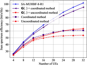
Finally, we showcase the generalization capability of SA-MUHBF by utilizing samples from region 2 and region 3 (see Fig. 7 for illustration) as testing samples. Notably, for the generalization test, SA-MUHBF is trained for the 8 UEs setup in region 1, denoted as SA-MUHBF-8-R1. The prediction NMSEs of ${\mathbf{G}}(\cdot)$ for SA-MUHBF-8-R1 on the samples from region 2 and region 3 are $0.1843$ and $0.1612$, respectively. Furthermore, Fig. 12 illustrates the sum spectrum efficiency of SA-MUHBF, along with the aforementioned baseline algorithms, on the testing samples from regions 2 and 3. As depicted, SA-MUHBF surpasses all baseline algorithms, demonstrating gains of 1.6% at 4 UEs, 4.9% at 8 UEs, 5.5% at 8 UEs, and 8.0% at 32 UEs on the testing samples from region 2, and gains of 2.5% at 4 UEs, 3.7% at 8 UEs, 5.1% at 16 UEs, and 6.7% at 32 UEs on the testing samples from region 3, over the best performing baseline. These results indicate that SA-MUHBF possesses considerable generalization capacity to unseen communication scenarios, which can be attributed to the structuring and training of ${\mathbf{S}}(\cdot)$ under a ”learning and optimization” paradigm, as discussed in Sec. IV-B3.

(a)

(b)

Figure 12: Performance of SA-MUHBF for unseen regions: (a) evaluation with testing samples generated from BS 3 and region 2, (b) evaluation with testing samples generated from BS 16 and region 3.

VI Conclusion

In this work, we have exploited the spatial congruence between sub-6G channel and mmWave channel to facilitate the multi-user mmWave hybrid beamforming. A deep learning based framework, named SA-MUHBF, has been developed to achieve this end. SA-MUHBF utilizes a convolutional neural network to predict mmWave beamspace from sub-6G channel estimate, followed by a customized multi-layer graph neural network for analog beam selection and a LMMSE precoder for digital beamforming. Extensive numerical experiments validate the effectiveness of SA-MUHBF, demonstrating its superiority over several state-of-the-art benchmarks. Notably, SA-MUHBF requires minimal pilot overhead and exhibits robust performance across various system configurations and unseen scenarios.

References

- [1] C. Liu, M. Li, S. V. Hanly, P. Whiting, and I. B. Collings, “Millimeter-wave small cells: Base station discovery, beam alignment, and system design challenges,” IEEE Wireless Communications, vol. 25, no. 4, pp. 40–46, 2018.
- [2] A. Alkhateeb, O. El Ayach, G. Leus, and R. W. Heath, “Channel estimation and hybrid precoding for millimeter wave cellular systems,” IEEE Journal of Selected Topics in Signal Processing, vol. 8, no. 5, pp. 831–846, 2014.
- [3] R. W. Heath, N. González-Prelcic, S. Rangan, W. Roh, and A. M. Sayeed, “An overview of signal processing techniques for millimeter wave mimo systems,” IEEE Journal of Selected Topics in Signal Processing, vol. 10, no. 3, pp. 436–453, 2016.
- [4] F. Sohrabi and W. Yu, “Hybrid Digital and Analog Beamforming Design for Large-Scale Antenna Arrays,” IEEE Journal of Selected Topics in Signal Processing, vol. 10, no. 3, pp. 501–513, Apr. 2016.
- [5] A. Alkhateeb and R. W. Heath, “Frequency selective hybrid precoding for limited feedback millimeter wave systems,” IEEE Transactions on Communications, vol. 64, no. 5, pp. 1801–1818, 2016.
- [6] Q. Hu, Y. Cai, K. Kang, G. Yu, J. Hoydis, and Y. C. Eldar, “Two-Timescale End-to-End Learning for Channel Acquisition and Hybrid Precoding,” IEEE Journal on Selected Areas in Communications, vol. 40, no. 1, pp. 163–181, Jan. 2022.
- [7] A. Alkhateeb, G. Leus, and R. W. Heath, “Limited feedback hybrid precoding for multi-user millimeter wave systems,” IEEE transactions on wireless communications, vol. 14, no. 11, pp. 6481–6494, 2015.
- [8] S. S. Nair and S. Bhashyam, “Hybrid beamforming in mu-mimo using partial interfering beam feedback,” IEEE Communications Letters, vol. 24, no. 7, pp. 1548–1552, 2020.
- [9] A. M. Elbir and A. K. Papazafeiropoulos, “Hybrid precoding for multiuser millimeter wave massive mimo systems: A deep learning approach,” IEEE Transactions on Vehicular Technology, vol. 69, no. 1, pp. 552–563, 2019.
- [10] W. Jin, J. Zhang, C.-K. Wen, and S. Jin, “Model-driven deep learning for hybrid precoding in millimeter wave mu-mimo system,” IEEE Transactions on Communications, vol. 71, no. 10, pp. 5862–5876, 2023.
- [11] M. Peter, K. Sakaguchi, S. Jaeckel, S. Wu, M. Nekovee, J. Medbo, K. Haneda, S. Nguyen, R. Naderpour, J. Vehmas et al., “Measurement campaigns and initial channel models for preferred suitable frequency ranges,” Deliverable D2, vol. 1, p. 160, 2016.
- [12] M. K. Samimi and T. S. Rappaport, “3-d millimeter-wave statistical channel model for 5g wireless system design,” IEEE Transactions on Microwave Theory and Techniques, vol. 64, no. 7, pp. 2207–2225, 2016.
- [13] D. Dupleich, N. Han, A. Ebert, R. Müller, S. Ludwig, A. Artemenko, J. Eichinger, T. Geiss, G. Del Galdo, and R. Thomä, “From sub-6 ghz to mm-wave: Simultaneous multi-band characterization of propagation from measurements in industry scenarios,” in 2022 16th European Conference on Antennas and Propagation (EuCAP), 2022, pp. 1–5.
- [14] P. Kyösti, P. Zhang, A. Pärssinen, K. Haneda, P. Koivumäki, and W. Fan, “On the feasibility of out-of-band spatial channel information for millimeter-wave beam search,” IEEE Transactions on Antennas and Propagation, vol. 71, no. 5, pp. 4433–4443, 2023.
- [15] T. Nitsche, A. B. Flores, E. W. Knightly, and J. Widmer, “Steering with eyes closed: mm-wave beam steering without in-band measurement,” in 2015 IEEE Conference on Computer Communications (INFOCOM), 2015, pp. 2416–2424.
- [16] A. Ali, N. González-Prelcic, and R. W. Heath, “Estimating millimeter wave channels using out-of-band measurements,” in 2016 Information Theory and Applications Workshop (ITA), 2016, pp. 1–6.
- [17] A. Ali, N. González-Prelcic, and R. W. Heath, “Spatial covariance estimation for millimeter wave hybrid systems using out-of-band information,” IEEE Transactions on Wireless Communications, vol. 18, no. 12, pp. 5471–5485, 2019.
- [18] A. Ali, N. González-Prelcic, and R. W. Heath, “Millimeter wave beam-selection using out-of-band spatial information,” IEEE Transactions on Wireless Communications, vol. 17, no. 2, pp. 1038–1052, 2017.
- [19] M. Alrabeiah and A. Alkhateeb, “Deep learning for mmwave beam and blockage prediction using sub-6 ghz channels,” IEEE Transactions on Communications, vol. 68, no. 9, pp. 5504–5518, 2020.
- [20] W. Deng, M. Li, Y. Liu, M.-M. Zhao, and M. Lei, “Enhancing mmwave beam prediction through deep learning with sub-6 ghz channel estimate,” in 2024 IEEE Wireless Communications and Networking Conference (WCNC2024), 2024, pp. 1–6, accepted.
- [21] I. Chafaa, R. Negrel, E. V. Belmega, and M. Debbah, “Federated channel-beam mapping: from sub-6ghz to mmwave,” in 2021 IEEE Wireless Communications and Networking Conference Workshops (WCNCW), 2021, pp. 1–6.
- [22] K. Ma, D. He, H. Sun, and Z. Wang, “Deep learning assisted mmwave beam prediction with prior low-frequency information,” in ICC 2021-IEEE International Conference on Communications, 2021, pp. 1–6.
- [23] F. Maschietti, D. Gesbert, and P. de Kerret, “Coordinated Beam Selection in Millimeter Wave Multi-User MIMO using Out-of-Band Information,” in ICC 2019 - 2019 IEEE International Conference on Communications (ICC), 2019, pp. 1–6.
- [24] Z. Li, C. Zhang, I.-T. Lu, and X. Jia, “Hybrid Precoding Using Out-of-Band Spatial Information for Multi-User Multi-RF-Chain Millimeter Wave Systems,” IEEE Access, vol. 8, pp. 50 872–50 883, 2020.
- [25] J. Liu, X. Li, T. Fan, S. Lv, and M. Shi, “Collaborative management of resource allocation and precoding for dual-mode networks,” IEEE Transactions on Vehicular Technology, vol. 72, no. 8, pp. 10 879–10 893, 2023.
- [26] S. He, S. Xiong, Y. Ou, J. Zhang, J. Wang, Y. Huang, and Y. Zhang, “An overview on the application of graph neural networks in wireless networks,” IEEE Open Journal of the Communications Society, vol. 2, pp. 2547–2565, 2021.
- [27] Y. Shen, Y. Shi, J. Zhang, and K. B. Letaief, “Graph neural networks for scalable radio resource management: Architecture design and theoretical analysis,” IEEE Journal on Selected Areas in Communications, vol. 39, no. 1, pp. 101–115, 2020.
- [28] M. Lee, G. Yu, and G. Y. Li, “Graph embedding-based wireless link scheduling with few training samples,” IEEE Transactions on Wireless Communications, vol. 20, no. 4, pp. 2282–2294, 2020.
- [29] S. He, S. Xiong, W. Zhang, Y. Yang, J. Ren, and Y. Huang, “Gblinks: Gnn-based beam selection and link activation for ultra-dense d2d mmwave networks,” IEEE Transactions on Communications, vol. 70, no. 5, pp. 3451–3466, 2022.
- [30] W. Deng, Y. Liu, M. Li, and M. Lei, “Gnn-aided user association and beam selection for mmwave-integrated heterogeneous networks,” IEEE Wireless Communications Letters, vol. 12, no. 11, pp. 1836–1840, 2023.
- [31] A. Alkhateeb, “DeepMIMO: A generic deep learning dataset for millimeter wave and massive MIMO applications,” in Proc. of Information Theory and Applications Workshop (ITA), San Diego, CA, Feb 2019, pp. 1–8.
- [32] Remcom, “Wireless InSite,” http://www.remcom.com/wireless-insite.
- [33] A. Alkhateeb, G. Leus, and R. W. Heath, “Compressed sensing based multi-user millimeter wave systems: How many measurements are needed?” in 2015 IEEE international conference on acoustics, speech and signal processing (ICASSP), 2015, pp. 2909–2913.
- [34] Y. Bengio, A. Courville, and P. Vincent, “Representation learning: A review and new perspectives,” IEEE Transactions on Pattern Analysis and Machine Intelligence, vol. 35, no. 8, pp. 1798–1828, 2013.
- [35] Y. Shi, Z. Huang, S. Feng, H. Zhong, W. Wang, and Y. Sun, “Masked Label Prediction: Unified Message Passing Model for Semi-Supervised Classification,” in Proceedings of the Thirtieth International Joint Conference on Artificial Intelligence. Montreal, Canada: International Joint Conferences on Artificial Intelligence Organization, Aug. 2021, pp. 1548–1554.
- [36] D. H. Nguyen and T. Le-Ngoc, “Mmse precoding for multiuser miso downlink transmission with non-homogeneous user snr conditions,” EURASIP Journal on Advances in Signal Processing, vol. 2014, no. 1, pp. 1–12, 2014.
- [37] “ReduceLROnPlateau — PyTorch 2.1 documentation.” [Online]. Available: https://pytorch.org/docs/stable/generated/torch.optim.lr_scheduler.ReduceLROnPlateau.html