stMCDI: Masked Conditional Diffusion Model with Graph Neural Network for Spatial Transcriptomics Data Imputation

Abstract

Spatially resolved transcriptomics represents a significant advancement in single-cell analysis by offering both gene expression data and their corresponding physical locations. However, this high degree of spatial resolution entails a drawback, as the resulting spatial transcriptomic data at the cellular level is notably plagued by a high incidence of missing values. Furthermore, most existing imputation methods either overlook the spatial information between spots or compromise the overall gene expression data distribution. To address these challenges, our primary focus is on effectively utilizing the spatial location information within spatial transcriptomic data to impute missing values, while preserving the overall data distribution. We introduce stMCDI, a novel conditional diffusion model for spatial transcriptomics data imputation, which employs a denoising network trained using randomly masked data portions as guidance, with the unmasked data serving as conditions. Additionally, it utilizes a GNN encoder to integrate the spatial position information, thereby enhancing model performance. The results obtained from spatial transcriptomics datasets elucidate the performance of our methods relative to existing approaches.

1 Introduction

Spatial transcriptomics has revolutionized our understanding of cellular communication and functionality within specific microenvironments. This technology facilitates the precise localization of cells within tissues, crucial for elucidating tissue structure and function, and has significantly advanced single-cell biomics analysis Buenrostro et al. (2015); Burgess (2019). However, the high resolution inherent in spatial transcriptomics also introduces certain limitations Moses and Pachter (2022). The low RNA capture rate of this sequencing method potentially limits its ability to detect a wide range of genes, often resulting in data with numerous missing values. Consequently, researchers have developed imputation methods to accurately estimate missing data values, thereby enhancing data quality Figueroa-García et al. (2023); Sousa da Mota et al. (2023); Telyatnikov and Scardapane (2023). In recent years, there has been a significant surge in the development of imputation techniques for spatial transcriptomics data. These techniques primarily encompass generative probabilistic models, matrix factorization, and deep learning models Eraslan et al. (2019); Huang et al. (2018); Li and Li (2018).

Advancements in the field of missing data imputation are particularly notable in computer vision and natural language processing. However, accurately imputing spatial transcriptomics data continues to pose significant challenges. Traditional methods are inadequate, as they frequently overlook crucial spatial information, merely reconstructing gene expression matrices Talwar et al. (2018). To address this issue, recent research has shifted towards a graph-based approach Wang et al. (2021); Deng et al. (2023), leveraging spatial location information in spatial transcriptomics data. This methodology Kong et al. (2023); Gao et al. (2023) constructs a graph using spatial location data and employs a graph neural network for processing. While this approach incorporates spatial information, it can potentially distort data distribution, leading to suboptimal imputation results. Furthermore, the absence of true labels for spatial transcriptomics data complicates the assessment of imputation accuracy. In the fields of computer vision and natural language processing, self-supervised learning is frequently employed to compensate for the lack of real labels. Consequently, developing an effective imputation method to manage missing spatial transcriptomics data represents a critical challenge that requires resolution.

In this paper, we introduce a novel method for spatial transcriptomics data imputation, stMCDI. Our method leverages spatial position information to construct a graph about the spot. This graph is then used by a graph neural network to learn a latent representation, incorporating spatial position information. To address the challenge of working without labels, our approach is inspired by techniques from related research He et al. (2022); Hou et al. (2022). We mask a portion of the original data values, rendering them invisible to the GNN encoder. This masking step is crucial for our training process. We then apply a re-masking technique to the latent representation and employ a conditional score-based diffusion model for training the denoising network. The unmasked part of the data serves as a prior condition during this training phase. Additionally, the re-masked part undergoes processing by our training diffusion model.

We highlight the main contribution as follows:

• We employ a graph encoder to integrate gene expression matrices with spatial location information from spatial transcriptomic data.

• Employing a masked strategy, our model can predict unknown segments based on known data segments, thereby enhancing imputation performance. Simultaneously, it functions as a self-supervised learning method, providing corresponding labels for the model.

• Utilizing the conditional diffusion model, the known segment of the data is incorporated as a priori conditions into the diffusion model, thereby enhancing the model’s ability to align with the data’s distribution and improving imputation performance.

2 Related Work

2.1 Self-supervised Learning for Data Imputation

Self-supervised learning, which effectively utilizes large amounts of unlabeled data, has gained tremendous attention across various fields. In NLP field, for instance, self-supervised models have shown remarkable capability in learning rich data representations without relying on labeled data Kenton and Toutanova (2019); Brown et al. (2020). In time series imputation and prediction, this method involves masking or modifying data segments. Models are trained to predict or reconstruct this missing data, thereby learning the underlying data distribution. Tipirneni and Reddy (2022); Fortuin et al. (2020a); Luo et al. (2018). In image processing, self-supervised learning is vital for tasks like denoising and repairing images. A typical method involves masking parts of an image, with the model learning to fill these gaps, thereby improving its understanding of spatial context and image representation. Huang et al. (2021); Xie et al. (2020).

2.2 Imputation Data via Generative Model

Deep generative models, such as GANs and VAEs, are increasingly central in research for imputing missing data. The GAIN framework, a novel approach utilizing adversarial training, capitalizes on the capability of GANs to generate realistic data distributions Yoon et al. (2018). This enables GAIN to effectively impute missing data, ensuring consistency with the observed data. Similarly, VAEs, with their probabilistic foundations and ability to handle complex distributions, are adept at learning the data’s underlying representation, making them vital for data imputation Fortuin et al. (2020b). Utilizing generative models for data imputation poses challenges, including potential bias in cases of extensive missing data and interpretability issues due to their complexity, especially in sensitive areas like medical data handling Liu et al. (2023); Sun et al. (2023).

2.3 Spatial Transcriptomics Data Imputation

Spatial transcriptomics technology, known for providing both RNA expression patterns and their spatial information, has garnered significant interest Fang et al. (2023); Yarlagadda et al. (2023). Despite the rapid development of improved techniques in this field, those that aim to offer comprehensive spatial transcriptome-level profiles face challenges, notably dropout problems stemming from high rates of missing data. Addressing this, the strategy of data imputation has emerged as a key method to mitigate these technical issues. There are currently several common imputation methods, such as SpaGE Abdelaal et al. (2020), stPlus Shengquan et al. (2021), gimVI Lopez et al. (2019), Tangram Biancalani et al. (2021). However, the performance of several common methods was lower than expected, indicating that there is still a gap in imputation tools for handling missing events in spatially resolved transcriptomics.

3 Proposed Method: stMCDI

We propose a conditional diffusion model, stMCDI, for spatial transcriptomic data imputation (Figure 1). The model is able to perform accurate imputation using the spatial position information of the idling data as well as the information available in the observations.

3.1 Problem formulation

In our problem, we work with two types of input data: the gene expression matrix $X=\{x_{i}\}_{i}^{n}\in\mathbb{R}^{n\times p}$ and the spatial location information of spots $C\in\mathbb{R}^{n\times 2}$. Here, $n$ represents the number of spots and $p$ represents the number of gene features. In the gene expression matrix $X$, some gene expressions are incomplete due to limitations in sequencing technology. To address this, we define $X$ as $X=X^{c}\cup X^{*}$, where $X^{c}$ represents the known part of the data and $X^{*}$ represents the missing part. Our objective is to develop an imputation function $\mathcal{F}:X\rightarrow\bar{X}$, which transforms $X$ with its missing values into a complete matrix $\bar{X}$ without any missing values. This function, $\mathcal{F}$, aims to accurately estimate and replace the missing values. In contrast to traditional diffusion model applications where vast amounts of data are typically available, our research field often deals with limited datasets. Consequently, we treat each spot as an individual sample. The strategy is to predict the missing parts of each spot by understanding and utilizing the unique data distribution characteristics of each spot.

To evaluate the performance of $\mathcal{F}$, we use four key evaluation metrics: Pearson Correlation Coefficient (PCC), Cosine Similarity (CS), Root Mean Square Error (RMSE), and Mean Absolute Error (MAE). For more details about the evaluation indicators, please refer to the Appendix D.

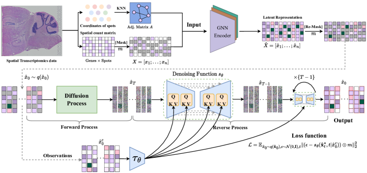
Figure 1: The network architecture of the proposed stMCDI model. Our model input has two parts: spot gene expression matrix and spot spatial location information. Build a graph based on the location information of each adjacent spot. Then the diffusion model is used to restore the masked representation to achieve the purpose of imputation.

3.2 Mask and re-mask strategy in stMCDI

Since spatial transcriptomic data lacks labels, we adopt a self-supervised learning approach. This method involves initially masking a portion of the original data for two key purposes: i) The masked part of the data serves as a pseudo label for subsequent use, allowing for the calculation of various evaluation indicators. ii) Masking a portion of the data enables the GNN encoder to better fit the deep distribution and semantic structure during the training process, as the model learns to predict the missing information. Inspired by how large language models comprehend context, we apply a re-masking technique to the latent representation reconstructed by the GNN encoder. This is done for two primary reasons: i) To improve the model’s ability to predict data gradient distribution. ii) To use the unmasked part as a prior condition, guiding the diffusion model in restoring the masked portion and thus enhancing the model’s overall performance.

3.3 GNN Encoder in stMCDI for integrating ST location information

3.3.1 Constructing adjacency matrices

Since spatial transcriptomic data lacks inherent graph structure, we manually construct an adjacency matrix to better utilize its spatial location information. In this matrix, the spatial position of each spot is represented in two dimensions. To determine the connections between spots, we calculate the Euclidean distance between each pair of spots, $p_{i}=(x_{i},y_{i})$ and $p_{j}=(x_{j},y_{j})$. The distance $d$ between them is given by:

$$d_{ij}=\sqrt{(x_{i}-x_{j})^{2}+(y_{i}-y_{j})^{2}}.$$ (1)

This distance calculation helps us in constructing the adjacency matrix. We establish adjacency edges between each spot and its five closest neighbors, resulting in the adjacency matrix $\mathbf{A}$. In $\mathbf{A}$, the elements $\mathbf{A}_{ij}$ are defined as follows:

$$A_{ij}=\begin{cases}1,&\text{if there is an edge between }\text{spot}~{}i\text{ and }j\\ 0,&\text{otherwise}\end{cases}$$ (2)

3.3.2 Constructing latent representation with GCN

In spatial transcriptomic data analysis, effectively utilizing spatial location information is crucial. To achieve this, we implement a graph convolutional network (GCN) as an encoder. The GCN encoder integrates information from neighboring spots. This ensures that the gene expression characteristics of each spot are not considered in isolation but are blended with those of its adjacent neighbors. Through this integration, we achieve multi-scale fusion of gene expression data, thereby enhancing the richness and semantic depth of gene expression information. As a result, it produces an enriched overall representation of the data, characterized by enhanced informational content and greater biological significance. The building of latent representations in the GCN encoder is defined as follows:

$$\begin{split}&\hat{X}=GCN(X,\mathbf{A}),\\ &\hat{X}=(\hat{x}_{1},\dots,\hat{x}_{n}),~{}X=(x_{1},\dots,x_{n}).\end{split}$$ (3)

Among them, $\mathbf{X}$ represents the gene expression matrix, $\mathbf{\hat{X}}$ represents the reconstructed latent representation matrix, and $\mathbf{A}$ is the constructed adjacency matrix.

3.4 Conditional score-based diffusion model in stMCDI

3.4.1 Denoising diffusion probabilistic model and Score-based diffusion model

In the realm of denoising diffusion probabilistic models Sohl-Dickstein et al. (2015); Ho et al. (2020), consider the task of learning a model distribution $p_{\theta}(\mathbf{x}_{0})$ that closely approximates a given data distribution $q(\mathbf{x}_{0})$. Suppose we have a sequence of latent variables $\mathbf{x}_{t}$ for $t=1,\ldots,T$, existing within the same sample space as $\mathbf{x}_{0}$, which is denoted as $\mathcal{X}$. DDPMs are latent variable models that are composed of two primary processes: the forward process and the reverse process. The forward process is defined by a Markov chain, described as follows:

$$\begin{split}&q(\mathbf{x}_{1:T}|\mathbf{x}_{0}):=\prod_{t=1}^{T}q(\mathbf{x}_{t}|\mathbf{x}_{t-1}),\\ \text{where }&q(\mathbf{x}_{t}|\mathbf{x}_{t-1}):=\mathcal{N}(\sqrt{1-\beta_{t}}\mathbf{x}_{t-1},\beta_{t}\mathbf{I}).\end{split}$$ (4)

and the variable $\beta_{t}$ is a small positive constant indicative of a noise level. The sampling of $x_{t}$ can be described by the closed-form expression $q(x_{t}|x_{0})=\mathcal{N}(x_{t};\sqrt{\alpha_{t}}x_{0},(1-\alpha_{t})\mathbf{I})$, where $\hat{\alpha}_{t}:=1-\beta_{t}$ and $\alpha_{t}$ is the cumulative product $\alpha_{t}:=\prod_{i=1}^{t}\hat{\alpha}_{i}$. Consequently, $x_{t}$ is given by the equation $x_{t}=\sqrt{\alpha_{t}}x_{0}+(1-\alpha_{t})\epsilon$, with $\epsilon\sim\mathcal{N}(0,\mathbf{I})$. In contrast, the reverse process aims to denoise $x_{t}$ to retrieve $x_{0}$, a process which is characterized by the ensuing Markov chain:

$$p_{\theta}(\mathbf{x}_{0:T}):=p(\mathbf{x}_{T})\prod_{t=1}^{T}p_{\theta}(\mathbf{x}_{t-1}|\mathbf{x}_{t}),\quad\mathbf{x}_{T}\sim\mathcal{N}(0,\mathbf{I}),$$ (5)

$$p_{\theta}(\mathbf{x}_{t-1}|\mathbf{x}_{t}):=\mathcal{N}(\mathbf{x}_{t-1};\mu_{\theta}(\mathbf{x}_{t},t),\sigma^{2}_{\theta}(\mathbf{x}_{t},t)\mathbf{I}),$$

$$\mu_{\theta}(\mathbf{x}_{t},t)=\frac{1}{\alpha_{t}}\left(\mathbf{x}_{t}-\frac{\beta_{t}}{\sqrt{1-\alpha_{t}}}\epsilon_{\theta}(\mathbf{x}_{t},t)\right),$$

$$\sigma_{\theta}(\mathbf{x}_{t},t)=\beta_{t}^{1/2},$$

$$\text{where }\beta_{t}=\begin{cases}\frac{1-\bar{\alpha}_{t-1}}{1-\bar{\alpha}_{t}}\beta_{1},&\text{for }t>1,\\ \beta_{1},&\text{for }t=1,\end{cases}$$

$$\text{and }\epsilon_{\theta}(\mathbf{x}_{t},t)\text{ is a trainable denoising function.}$$

In our proposed method, we use a score-based diffusion model, whose main difference from the traditional DDPM is the different coefficients in the sampling stage. Due to space limitations, specific derivation can be found in Appendix A.1.

3.4.2 Conditioning mechanisms in stMCDI

The method we propose aims to estimate the entire dataset by using the known data as a priori conditions. This approach is designed to effectively achieve the purpose of data imputation in spatial transcriptomic analysis. By leveraging the existing known data, our model can infer the missing values, thereby reconstructing a complete and accurate representation of the entire dataset. We denote the observed (unmasked) data as $x_{j,0}^{c}=m\odot x_{j,0}$, where $x_{j,0}$ mean the $j^{\text{th}}$ sample in 0 step, and $\odot$ denotes matrix element-wise multiplication and $m\in\{0,1\}^{n\times 1}$ is the elemen-wise indicator with ones be observed and zeros be masked. So, our goal is to estimate the posterior $p((E_{n,1}-m)\odot x|M\odot x)$, where $E_{n,1}$ is all-ones matrix of dimensions $n\times 1$. We also denote the imputation data as $x_{j,t}^{*}$, where t is time step. Therefore, our conditional mechanisms in stMCDI’s objective is to estimate the probabilistic:

$$p_{\theta}(x_{j,t-1}^{*}|x_{j,t}^{*},x_{j,0}^{c}).$$ (6)

In order to better use the observed values as a priori conditions for the diffusion model to perform missing value imputation, we transform the Eq. (4) and Eq. (5) into:

$$\small\begin{split}&p_{\theta}(x_{j,0:T}^{*}|x_{j,0}^{c}):=p(x_{j,T}^{*})\prod_{t=1}^{T}p_{\theta}(x_{j,t-1}^{*}|x_{j,t}^{*},x_{j,0}^{c}),x_{j,T}^{*}\sim\mathcal{N}(0,\mathbf{I}).\\ &p_{\theta}(x_{j,t-1}^{*}|x_{j,t}^{*},x_{j,0}^{c}):=\mathcal{N}(x_{j,t-1}^{*};\mu_{\theta}(x_{j,t}^{*},t|x_{j,0}^{c}),\sigma_{\theta}(x_{j,t}^{*},t|x_{j,0}^{c})\mathbf{I}).\end{split}$$ (7)

We can optimize the Eq. (7) parameters by minimizing the variational lower bound:

$$\small\mathbb{E}_{q}\left[-\log p_{\theta}(x_{j,0}\mid x_{j,0}^{c})\right]\leq\mathbb{E}_{q}\left[-\log\frac{p_{\theta}(x_{j,0:T}\mid x_{j,0}^{c})}{q(x_{j,1:T}\mid x_{j,0})}\right].$$ (8)

Also we can get a simplified training objective:

$$\mathbb{E}_{x_{j,0}\sim q(\mathbf{x}_{j,0}),\epsilon\sim\mathcal{N}(0,\mathbf{I}),t}\|(\epsilon-s_{\theta}(\mathbf{x}_{j,t}^{*},t|x_{j,0}^{c}))\|^{2}_{2}.$$ (9)

The goal of conditioner $\tau_{\theta}$ is a multilayer perceptron (MLP) that converts unmasked part of data as an input condition $\tau_{\theta}(x_{j,0}^{c})$. Inspired by other generative models, the diffusion model essentially models a conditional distribution of the form $p(z|y)$, where $y$ is a prior condition. This can be achieved by training a conditional denoising function $s_{\theta}(x_{j,t},t,y)$, and controlling the generation of the final target by inputting the condition $y$. We enhance the underlying UNet’s Backbone through the cross-attention mechanism, turning SDM into a more flexible conditional diffusion model, allowing us to better learn the gradient distribution of data, thereby restoring a data distribution without missing. We introduce a specific encoder $\tau_{\theta}$, which projects the representation except the mask part to the intermediate representation $\tau_{\theta}(x_{j,0}^{c})$, and then maps it to the intermediate layers of the UNet through the cross attention layer:

$$\begin{split}&\text{Attenntion}(Q,K,V)=\text{softmax}\left(\frac{QK^{T}}{\sqrt{d}}\right)\cdot V,\text{with}\\ &Q=W_{Q}^{(i)}\cdot\varphi_{i}(x_{j,T}^{*}),K=W_{K}^{(i)}\cdot\tau_{\theta}(x_{j,0}^{c}),V=W_{V}^{(i)}\cdot\tau_{\theta}(x_{j,0}^{c})\end{split}$$ (10)

In this place equation, $\varphi_{i}(x_{j,T}^{*})$ denotes a intermediate representation of the UNet implementing $\epsilon_{\theta}$ and $W_{Q}^{(i)},W_{K}^{(i)},W_{V}^{(i)}$ are learnable projection metrices.

3.4.3 Imputation with stMCDI

We focus on refining the conditional diffusion model characterized by the reverse process described in Eq. (7). Our goal is to accurately model the conditional distribution $p\left(x_{j,t-1}^{*}|x_{j,t}^{*},x_{j,0}^{c}\right)$ without resorting to approximations. To achieve this, we adapt the parameterization of DDPM from Eq. (5) for the conditional setting. We introduce a conditional denoising function $s_{\theta}:\left(\mathcal{X}^{*}\times\mathbb{R}\mid\mathcal{X}^{c}\right)\rightarrow\mathcal{X}^{*}$ that accepts the conditional observations $x_{j,0}^{c}$ as input parameters. Building on this, we employ the parameterization with $\epsilon_{\theta}$ as follows:

$$\begin{split}\mu_{\theta}(x_{j,t}^{*},t|x_{j,0}^{c})&=\mu^{\text{Score-based}}\left(x_{j,t}^{*},t,s_{\theta}\left(x_{j,t}^{*},t|x_{j,0}^{c}\right)\right),\\ \sigma_{\theta}(x_{j,t}^{*},t|x_{j,0}^{c})&=\sigma^{\text{Score-based}}\left(x_{j,t}^{*},t\right),\end{split}$$ (11)

where $\mu^{\text{Score-based}}$ and $\sigma^{\text{Score-based}}$ are defined in Section 3.4.1. Utilizing the function $\epsilon_{\theta}$ and the data $x_{0}$, we can simulate samples of $x_{j,0}^{*}$ by employing the reverse process outlined in Eq. (7). During sampling, we treat the known values of $x_{j,0}$ as the conditional observations $x_{j,0}^{c}$ and the unknown values as the targets for imputation $x_{j,0}^{*}$.

3.5 Loss function of stMCDI

Specifically, in the presence of conditional observations $x_{j,0}^{c}$ and imputation targets $x_{j,0}^{*}$, we generate noisy targets $x_{j,t}^{*}=\sqrt{\alpha_{t}}x_{j,0}^{*}+\sqrt{(1-\alpha_{t})}\epsilon$, and proceed to refine $s_{\theta}$ by minimizing the ensuing loss function:

$$\mathcal{L}=\mathbb{E}_{x_{j,0}\sim q(\mathbf{x}_{j,0}),\epsilon\sim\mathcal{N}(0,\mathbf{I}),t}\|(\epsilon-s_{\theta}(\mathbf{x}_{j,t}^{*},t|x_{j,0}^{c}))\odot M\|^{2}_{2}.$$ (12)

The stMCDI algorithm framework can be found in the Appendix B.

4 Experiment

4.1 Data sources and data preprocessing

We compared the performance of our model with other baseline methods on 6 real-world spatial transcriptomic datasets from several representative sequencing platforms. The real-world spatial transcriptomics datasets, including: Mouse Olfactory Bulb (MOB), Human Breast Cancer (HBC), Human Prostate (HP), Human Osteosarcoma (HO), Mouse Liver (ML), Mouse Kidney (MK), used in our experiments were derived from recently published papers on spatial transcriptomics experiments, and our data preprocessing method is consistent with this paper Li et al. (2022). All datasets come from different species, including mice and humans, and different organs, such as liver and kidneys. Specifically, the number of spots ranges from 278 to 6000, and the gene range ranges from 14192 to 28601. Detailed information about the dataset can be found in the Appendix E.

Method	Dataset_1: Mouse Olfactory Bulb (MOB)				Dataset_2: Human Breast Cancer (HBC)				Dataset_3: Human Prostate (HP)
	PCC$\uparrow$	Cosine$\uparrow$	RMSE$\downarrow$	MAE$\downarrow$	PCC$\uparrow$	Cosine$\uparrow$	RMSE$\downarrow$	MAE$\downarrow$	PCC$\uparrow$	Cosine$\uparrow$	RMSE$\downarrow$	MAE$\downarrow$
Mean	-0.005±0	0.037±0	1.334±0	1.013±0	-0.223±0	-0.476±0	0.973±0	0.884±0	-0.632±0	-0.237±0	1.731±0	1.603±0
KNN	-0.063±0.0012	0.094±0.0018	1.103±0.0357	0.953±0.0027	-0.371±0.0001	0.148±0.0001	0.812±0.0002	0.741±0.0001	-0.0034±0.0017	0.223±0.0022	0.971±0.0005	0.843±0.0007
gimVI	0.513±0.0013	0.477±0.0011	0.346±0.0022	0.241±0.0005	0.538±0.0006	0.461±0.0006	0.460±0.0004	0.406±0.0012	0.615±0.0002	0.619±0.0007	0.461±0.0019	0.437±0.0022
SpaGE	0.436±0.0026	0.503±0.0007	0.289±0.0003	0.256±0.0012	0.578±0.0004	0.513±0.0004	0.413±0.0011	0.389±0.0007	0.634±0.0013	0.603±0.0024	0.423±0.0021	0.488±0.0007
Tangram	0.603±0.0002	0.526±0.0004	0.203±0.0002	0.301±0.00021	0.603±0.0014	0.525±0.0001	0.396±0.0021	0.351±0.0002	0.657±0.0022	0.611±0.0017	0.401±0.0005	0.396±0.0006
stPlus	0.611±0.0003	0.518±0.0002	0.301±0.0004	0.212±0.0016	0.651±0.0002	0.534±0.0004	0.387±0.0012	0.404±0.0005	0.587±0.001	0.663±0.0021	0.469±0.0007	0.357±0.0221
STAGATE	0.626±0.0021	0.536±0.0034	0.242±0.0014	0.196±0.0026	0.626±0.0004	0.503±0.0002	0.401±0.0002	0.363±0.0004	0.626±0.0002	0.653±0.0002	0.403±0.0017	0.326±0.0004
DCA	0.465±0.0029	0.491±0.0047	0.338±0.0009	0.289±0.0013	0.460±0.0009	0.437±0.0011	0.483±0.0024	0.461±0.0024	0.559±0.0003	0.572±0.0006	0.509±0.0004	0.496±0.0004
GraphSCI	0.408±0.0026	0.509±0.0006	0.355±0.0009	0.329±0.0006	0.481±0.0006	0.437±0.0002	0.504±0.0005	0.476±0.0011	0.565±0.0014	0.551±0.0003	0.479±0.0003	0.453±0.0005
SpaFormer	0.385±0.0013	0.336±0.0016	0.505±0.0077	0.343±0.0004	0.375±0.0002	0.381±0.0004	0.632±0.0009	0.515±0.0003	0.537±0.0031	0.453±0.0006	0.607±0.0028	0.598±0.0025
CpG	0.627±0.0017	0.511±0.0004	0.321±0.0015	0.248±0.0004	0.475±0.0003	0.440±0.0009	0.460±0.0001	0.413±0.0001	0.589±0.0014	0.445±0.0061	0.587±0.0024	0.563±0.0019
GraphCpG	0.557±0.0003	0.539±0.0009	0.288±0.0002	0.243±0.0003	0.501±0.0001	0.443±0.0017	0.436±0.0016	0.403±0.0022	0.629±0.0003	0.459±0.0041	0.531±0.0013	0.518±0.0005
scGNN	0.548±0.0005	0.532±0.0007	0.307±0.0009	0.244±0.0011	0.502±0.0015	0.455±0.0019	0.437±0.0083	0.389±0.0015	0.602±0.0007	0.468±0.0033	0.479±0.0007	0.502±0.0004
CSDI	0.555±0.0008	0.529±0.0008	0.293±0.0002	0.216±0.0018	0.495±0.0004	0.481±0.0079	0.395±0.0004	0.379±0.0006	0.624±0.0005	0.569±0.0014	0.497±0.0051	0.484±0.0043
stMCDI (Ours)	0.645±0.0004	0.557±0.0018	0.188±0.0002	0.147±0.0012	0.703±0.0003	0.623±0.0012	0.304±0.0017	0.332±0.0027	0.714±0.0018	0.726±0.0022	0.367±0.0023	0.316±0.0007
Method	Dataset_4: Human Osteosarcoma (HO)				Dataset_5: Mouse Liver (ML)				Dataset_6: Mouse Kidney (MK)
	PCC$\uparrow$	Cosine$\uparrow$	RMSE$\downarrow$	MAE$\downarrow$	PCC$\uparrow$	Cosine$\uparrow$	RMSE$\downarrow$	MAE$\downarrow$	PCC$\uparrow$	Cosine$\uparrow$	RMSE$\downarrow$	MAE$\downarrow$
Mean	0.136±0	-0.469±0	1.264±0	1.033±0	0.047±0	0.024±0	1.337±0	1.454±0	0.047±0	0.024±0	1.337±0	1.454±0
KNN	0.157±0.0004	0.147±0.0081	1.081±0.0081	0.958±0.0018	0.227±0.0017	0.117±0.0041	0.947±0.0005	1.013±0.0032	0.227±0.0017	0.117±0.0041	0.947±0.0005	1.013±0.0032
gimVI	0.454±0.0005	0.642±0.0011	0.487±0.0011	0.436±0.0009	0.379±0.0043	0.219±0.0055	0.412±0.0003	0.467±0.0022	0.459±0.0004	0.344±0.0054	0.546±0.0018	0.526±0.0026
SpaGE	0.489±0.0005	0.613±0.0028	0.433±0.0004	0.389±0.0004	0.315±0.0026	0.289±0.0037	0.403±0.0079	0.496±0.0047	0.503±0.0007	0.447±0.0001	0.567±0.0011	0.515±0.0007
Tangram	0.396±0.0127	0.637±0.0017	0.467±0.0121	0.403±0.0002	0.403±0.0017	0.361±0.0051	0.379±0.0021	0.422±0.0031	0.489±0.0022	0.473±0.0003	0.476±0.0006	0.489±0.0013
stPlus	0.481±0.0056	0.625±0.0026	0.489±0.0025	0.357±0.0001	0.511±0.0022	0.401±0.0004	0.401±0.0007	0.378±0.0003	0.522±0.0031	0.563±0.0013	0.516±0.0081	0.441±0.0079
STAGATE	0.591±0.0013	0.676±0.0027	0.466±0.0022	0.401±0.0003	0.536±0.0013	0.489±0.0107	0.467±0.0026	0.439±0.0011	0.679±0.0028	0.611±0.0023	0.361±0.0002	0.379±0.0004
DCA	0.401±0.0032	0.571±0.0018	0.467±0.0018	0.441±0.0014	0.488±0.0029	0.463±0.0061	0.432±0.0079	0.504±0.0078	0.537±0.0016	0.638±0.0084	0.413±0.0008	0.363±0.0006
GraphSCI	0.371±0.0061	0.605±0.0002	0.543±0.0014	0.524±0.0003	0.503±0.0011	0.537±0.0027	0.377±0.0025	0.412±0.0034	0.567±0.0004	0.604±0.0009	0.354±0.0004	0.323±0.0005
SpaFormer	0.374±0.0044	0.567±0.0048	0.558±0.0008	0.538±0.0009	0.575±0.0009	0.537±0.0016	0.411±0.0031	0.464±0.0007	0.426±0.0007	0.513±0.0009	0.503±0.0017	0.469±0.0053
CpG	0.425±0.0002	0.632±0.0004	0.564±0.0013	0.521±0.0005	0.603±0.0003	0.571±0.0072	0.481±0.0001	0.412±0.0009	0.517±0.0008	0.564±0.0006	0.431±0.0053	0.412±0.0007
GraphCpG	0.431±0.0016	0.619±0.0051	0.524±0.0031	0.558±0.0004	0.566±0.0003	0.467±0.0004	0.437±0.0053	0.423±0.0028	0.587±0.0056	0.729±0.0037	0.356±0.0076	0.388±0.0009
scGNN	0.431±0.0016	0.534±0.0004	0.524±0.0031	0.534±0.0004	0.423±0.0004	0.459±0.0001	0.397±0.0002	0.388±0.0017	0.439±0.0027	0.693±0.0018	0.347±0.0036	0.331±0.0051
CSDI	0.519±0.0007	0.642±0.0007	0.519±0.0003	0.478±0.0021	0.466±0.0005	0.465±0.0008	0.423±0.0007	0.401±0.0013	0.624±0.0015	0.743±0.0055	0.327±0.0016	0.304±0.0029
stMCDI (Ours)	0.689±0.0007	0.734±0.0028	0.401±0.0022	0.353±0.0013	0.632±0.0047	0.596±0.0004	0.389±0.0124	0.301±0.0004	0.737±0.0004	0.803±0.0019	0.312±0.0027	0.288±0.0042

Table 1: Performance comparison between various baselines on the spatial transcriptomic datasets using four evaluation metrics. Among them, the black bold part represents the best performance. It should be noted that KNN means to fill missing values using the nearest spot values. Mean means using the mean value of each spot to fill in missing values.

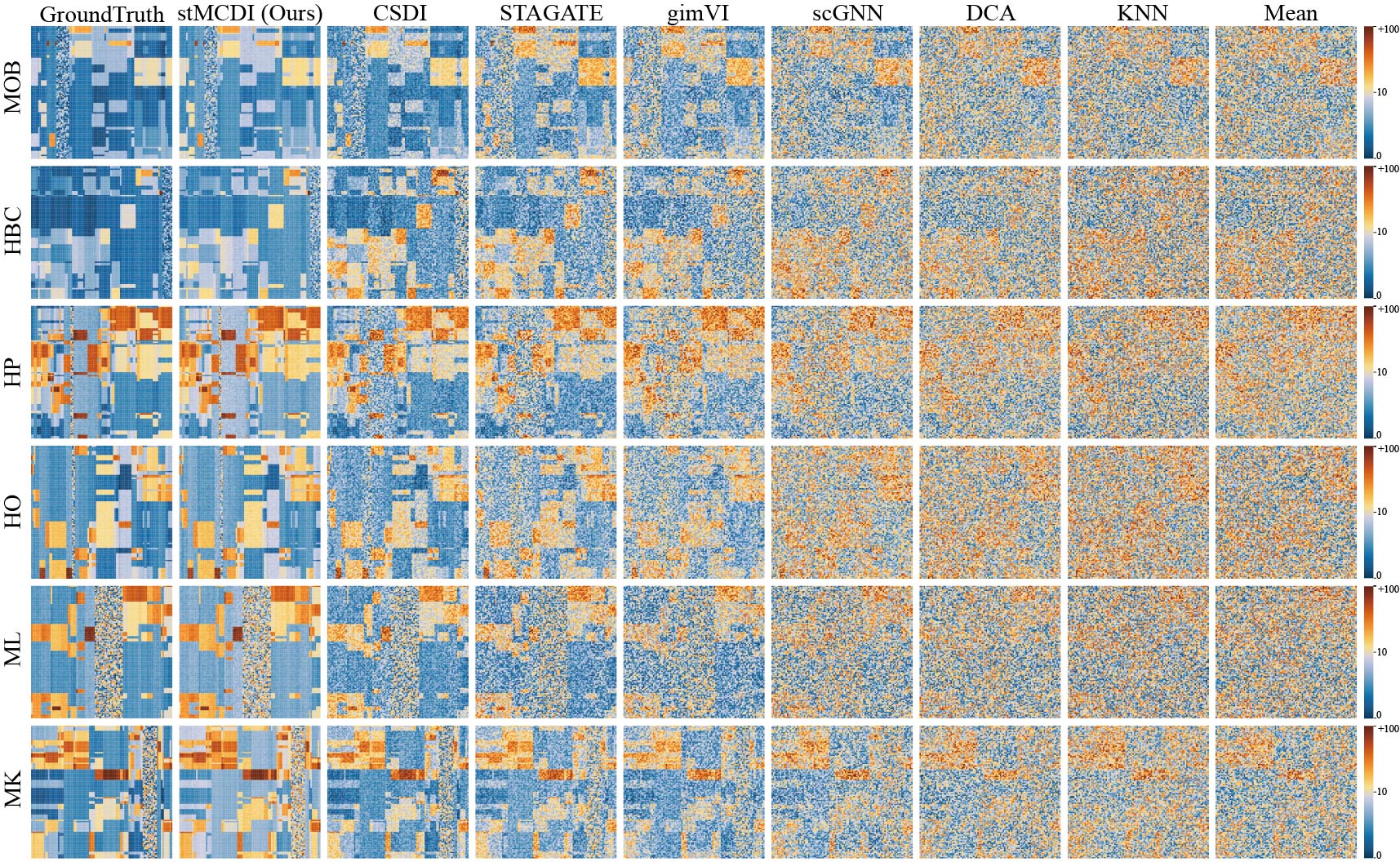
Figure 2: Visualization of the imputation performance of various baseline methods. In this figure, we only show several baselines: CSDI, STAGATE, gimVI, scGNN, DCA, KNN, Mean, etc. For the remaining Baslines, please refer to Appendix F.2.

4.2 Baselines

The performance of stMCDI was first compared with two regular imputation methods, including KNN imputation and mean imputation, as well as several state-of-the-art imputation methods for single-cell data and spatial transcriptomic data. Finally, we selected fourteen state-of-the-art methods for comparison:

• gimVI (Lopez et al. (2019)):It is a deep generative model for integrating spatial transcriptomics data and scRNA-seq data which can be used to impute missing genes.

• SpaGE (Abdelaal et al. (2020)):It is a method that integrates spatial and scRNA-seq datasets to predict whole-transcriptome expressions in their spatial configuration.

• Tangram (Biancalani et al. (2021)):It is a method that can map any type of sc/snRNA-seq data, including multimodal data such as those from SHARE-seq, which can be used to reveal spatial patterns of chromatin accessibility.

• stPlus (Shengquan et al. (2021)):It is a reference-based method that leverages information in scRNA-seq data to enhance spatial transcriptomics.

• STAGATE (Dong and Zhang (2022)):It is a method that adopts an attention mechanism to adaptively learn the similarity of neighboring spots, and an optional cell type-aware module through integrating the pre-clustering of gene expressions.

• DCA (Eraslan et al. (2019)):It is a deep count autoencoder network (DCA) to denoise scRNA-seq datasets.

• GraphSCI (Rao et al. (2021)):It is an imputation method (GraphSCI) to impute the dropout events in scRNA-seq data based on the graph convolution networks.

• SpaFormer (Wen et al. (2023)):It is a transformer-based imputation framework for cellular-level spatial transcriptomic data.

• CpG (De Waele et al. (2022)):It is a transformer-based imputation method to operate on methylation matrices through combining axial attention with sliding window self-attention.

• GraphCpG (Rao et al. (2021)):It is a novel graph-based deep learning approach to impute methylation matrices based on locus-aware neighboring subgraphs with locus-aware encoding orienting on one cell type.

• scGNN (Wang et al. (2021)):It is a hypothesis-free deep learning framework for scRNA-Seq imputations.

• CSDI (Tashiro et al. (2021)):It is a novel time series imputation method that utilizes score-based diffusion models conditioned on observed data.

4.3 Implementation Details

The hyperparameters of stMCDI are defined as follows: Graph encoder layers to 3 GCN layers; diffusion steps to 2000; learning rate to 6e-6; batch size to 64. The noise variances were in the range of 10-6 to 0.05. An exponential moving average (EMA) over model parameters with a rate of 0.926 emploved. The model is trained on 1 NVIDIA RTX 4090, 24 GB with Adamw optimizer on PyTorch. Specific details of each parameter can be found in the Appendix  C.

4.4 Results

We carry out multiple experiments on six real-world ST datasets with different the number of spots (Table 1). The experimental results demonstrate that our proposed method outperforms fourteen baseline methods, achieving the best performance across all four indicators.

To better demonstrate that our proposed method achieves state-of-the-art performance compared to other methods, we use a heatmap of gene expression to visualize the imputation results of stMCDI (as shown in Figure 2). We splice the mask part of each sample to form the real label, and we apply the same method to the imputation results of each baseline method. To enhance the visualization effect, we perform hierarchical clustering on the spliced mask gene expression matrix, making it exhibit more pronounced pattern-like features, thereby highlighting the effectiveness of the interpolation method. Due to space limitations, we only show part of the Baseline methods. More results can be found in the Appendix F.2.

4.5 Ablation studies

We conduct ablation experiment to verify the modules of stMCDI in these aspects: 1) Different Mask strategies and different Mask phase. 2) The impact of different Graph Encoder on model performance. 3) Different Mask ratios.

4.5.1 Different mask strategy and different mask phase

In our proposed method stMCDI, we randomly mask the gene expression matrix according to a certain proportion. We apply this masking process twice: once on the original input data and again on the intermediate latent representation. To demonstrate the effectiveness of our strategy, we conducted five controlled experiments. These experiments encompass two distinct Mask strategies: Mask Spot and Mask Gene, along with three different Mask phases: OR Mask (masking only the original data), LR Mask (masking only the latent representation), and NO Mask. The experimental results (Table 2) indicate that our approach is the most effective across six datasets. It also achieves superior performance in four key evaluation metrics compared to other methods.

Metrics	Dataset
PCC$\uparrow$	MOB	HBC	HP	HO	ML	MK
stMCDI (Ours)	0.645	0.703	0.714	0.689	0.632	0.737
w/ mask Spot	0.573	0.603	0.617	0.549	0.581	0.627
w/ mask Gene	0.588	0.612	0.626	0.567	0.593	0.643
w/o OR mask	0.624	0.656	0.677	0.626	0.611	0.639
w/o LR mask	0.602	0.633	0.659	0.587	0.628	0.614
w/o mask	0.569	0.527	0.496	0.533	0.588	0.601
Cosine$\uparrow$	MOB	HBC	HP	HO	ML	MK
stMCDI (Ours)	0.577	0.623	0.726	0.734	0.596	0.803
w/ mask Spot	0.511	0.561	0.641	0.681	0.503	0.731
w/ mask Gene	0.507	0.557	0.622	0.673	0.531	0.743
w/o OR mask	0.543	0.489	0.704	0.688	0.567	0.729
w/o LR mask	0.525	0.579	0.693	0.694	0.559	0.759
w/o mask	0.513	0.416	0.589	0.587	0.497	0.721
RMSE$\downarrow$	MOB	HBC	HP	HO	ML	MK
stMCDI (Ours)	0.188	0.304	0.367	0.401	0.389	0.312
w/ mask Spot	0.213	0.366	0.427	0.497	0.403	0.379
w/ mask Gene	0.224	0.372	0.438	0.503	0.411	0.406
w/o OR mask	0.215	0.403	0.363	0.459	0.464	0.413
w/o LR mask	0.202	0.358	0.422	0.445	0.451	0.439
w/o mask	0.307	0.402	0.379	0.488	0.426	0.415
MAE$\downarrow$	MOB	HBC	HP	HO	ML	MK
stMCDI (Ours)	0.147	0.332	0.316	0.353	0.301	0.288
w/ mask Spot	0.204	0.403	0.411	0.426	0.388	0.369
w/ mask Gene	0.211	0.397	0.423	0.437	0.426	0.403
w/o OR mask	0.164	0.384	0.386	0.439	0.453	0.366
w/o LR mask	0.195	0.362	0.398	0.415	0.437	0.482
w/o mask	0.288	0.401	0.417	0.441	0.449	0.467

Table 2: Ablation experiments on different masked strategy and different masked phase in stMCDI.

Metrics	Dataset
PCC$\uparrow$	MOB	HBC	HP	HO	ML	MK
stMCDI (Ours)	0.645	0.703	0.714	0.689	0.632	0.737
w/ GAT	0.597	0.501	0.655	0.578	0.607	0.688
w/ GIN	0.51	0.537	0.569	0.511	0.601	0.671
w/ MLP	0.505	0.517	0.526	0.488	0.579	0.665
w/o GNN	0.464	0.481	0.509	0.447	0.566	0.639
Cosine$\uparrow$	MOB	HBC	HP	HO	ML	MK
stMCDI (Ours)	0.557	0.623	0.726	0.734	0.596	0.803
w/ GAT	0.532	0.526	0.664	0.646	0.513	0.734
w/ GIN	0.514	0.507	0.613	0.598	0.501	0.705
w/ MLP	0.503	0.485	0.586	0.557	0.489	0.689
w/o GNN	0.489	0.426	0.537	0.521	0.457	0.655
RMSE$\downarrow$	MOB	HBC	HP	HO	ML	MK
stMCDI (Ours)	0.188	0.304	0.367	0.401	0.389	0.312
w/ GAT	0.308	0.398	0.411	0.452	0.402	0.374
w/ GIN	0.379	0.451	0.436	0.467	0.411	0.388
w/ MLP	0.431	0.512	0.565	0.493	0.423	0.404
w/o GNN	0.447	0.569	0.587	0.537	0.436	0.476
MAE$\downarrow$	MOB	HBC	HP	HO	ML	MK
stMCDI (Ours)	0.147	0.332	0.316	0.353	0.301	0.288
w/ GAT	0.188	0.367	0.413	0.413	0.359	0.326
w/ GIN	0.224	0.381	0.426	0.451	0.428	0.377
w/ MLP	0.289	0.405	0.435	0.467	0.446	0.389
w/o GNN	0.346	0.455	0.473	0.503	0.461	0.429

Table 3: Ablation experiments on different encoders of GNN. We tried different types of graph neural networks and found that GCN was the best graph encoder for our task.

4.5.2 Graph embedding with different graph neural network

Our stMCDI method includes a Graph embedding layer to enhance the processing of spatial position information in spatial transcriptomics data. This layer merges spatial data into the gene expression matrix, creating a graph with spatial characteristics. As a result, gene expression’s latent representation is augmented with adjacent position details, improving the data representation. To evaluate the efficiency of GNN in integrating spatial location information, we conducted a series of comparative studies. Our experimental results (Table 3) reveal that the GCN exhibits superior performance in our specific tasks. However, this finding does not diminish the effectiveness of other GNNs. Instead, it suggests that GCN is particularly well-suited for the specific requirements of our tasks.

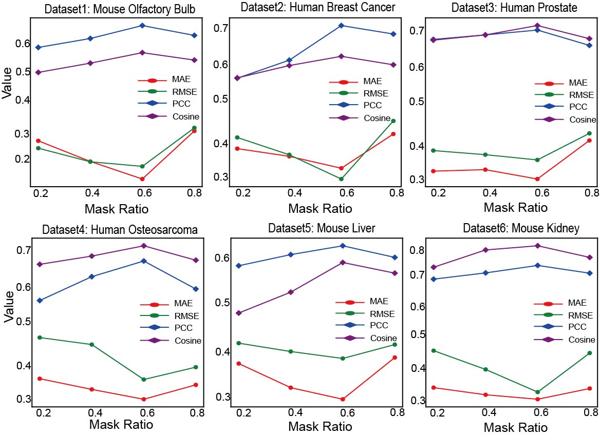
Figure 3: Different mask ratio of imputation performance in four metrics. We adopt different mask proportions for each sample, and we find that the performance of stMCDI reaches its best when the mask proportion is around 60%.

4.5.3 The impact of Mask ratio on model performance

In our method, the ratio of our mask is 60%, and we want to explore the impact of different mask ratios on the imputation performance of the model. We give the comparison of using different masking ratios in Figure 3. Therefore, we change the parameter mask ratio and observed the changes in model performance under different mask ratios. We found that as the mask ratio increases, the interpolation performance of the model decreases. The possible reason is that the model does not learn relevant representations from limited data.

5 Conclusion

In this paper, we propose a novel method: stMCDI, masked conditional diffusion model with graph neural network for spatial transcriptomics data imputation. By masking the latent representation and using the non-mask part as a condition, the diffusion model is well guided and controllable during reverse process, ensuring the quality of imputation. Experiments on the real spatial transcriptomic datasets show that our proposed method stMCDI achieves the best performance compared with other baselines. Moreover, ablation experiments demonstrate the effectiveness and reliability of our method. Although the stMCDI experimental results are promising, there is still a lot of scope for improvement. We can try multi-modal imputation methods, such as introducing single-cell data into the diffusion model as a priori conditions. Secondly, how the imputation data improves the performance of downstream analysis is still a question we consider.

Appendix

APPENDIX

Appendix A Details of denoising diffusion probabilistic models

A.1 Overview of DDPM and score-based model

In the realm of denoising diffusion probabilistic models Sohl-Dickstein et al. [2015]; Ho et al. [2020], consider the task of learning a model distribution $p_{\theta}(\mathbf{x}_{0})$ that closely approximates a given data distribution $q(\mathbf{x}_{0})$. Suppose we have a sequence of latent variables $\mathbf{x}_{t}$ for $t=1,\ldots,T$, existing within the same sample space as $\mathbf{x}_{0}$, which is denoted as $\mathcal{X}$. DDPMs are latent variable models that are composed of two primary processes: the forward process and the reverse process. The forward process is defined by a Markov chain, described as follows:

$$\begin{split}&q(\mathbf{x}_{1:T}|\mathbf{x}_{0}):=\prod_{t=1}^{T}q(\mathbf{x}_{t}|\mathbf{x}_{t-1}),\\ \text{where }&q(\mathbf{x}_{t}|\mathbf{x}_{t-1}):=\mathcal{N}(\sqrt{1-\beta_{t}}\mathbf{x}_{t-1},\beta_{t}\mathbf{I}),\end{split}$$ (13)

and the variable $\beta_{t}$ is a small positive constant indicative of a noise level. The sampling of $x_{t}$ can be described by the closed-form expression $q(x_{t}|x_{0})=\mathcal{N}(x_{t};\sqrt{\alpha_{t}}x_{0},(1-\alpha_{t})\mathbf{I})$, where $\hat{\alpha}_{t}:=1-\beta_{t}$ and $\alpha_{t}$ is the cumulative product $\alpha_{t}:=\prod_{i=1}^{t}\hat{\alpha}_{i}$. Consequently, $x_{t}$ is given by the equation $x_{t}=\sqrt{\alpha_{t}}x_{0}+(1-\alpha_{t})\epsilon$, with $\epsilon\sim\mathcal{N}(0,\mathbf{I})$. In contrast, the reverse process aims to denoise $x_{t}$ to retrieve $x_{0}$, a process which is characterized by the ensuing Markov chain:

$$p_{\theta}(\mathbf{x}_{0:T}):=p(\mathbf{x}_{T})\prod_{t=1}^{T}p_{\theta}(\mathbf{x}_{t-1}|\mathbf{x}_{t}),\quad\mathbf{x}_{T}\sim\mathcal{N}(0,\mathbf{I}),$$ (14)

$$p_{\theta}(\mathbf{x}_{t-1}|\mathbf{x}_{t}):=\mathcal{N}(\mathbf{x}_{t-1};\mu_{\theta}(\mathbf{x}_{t},t),\sigma^{2}_{\theta}(\mathbf{x}_{t},t)\mathbf{I}),$$

$$\mu_{\theta}(\mathbf{x}_{t},t)=\frac{1}{\alpha_{t}}\left(\mathbf{x}_{t}-\frac{\beta_{t}}{\sqrt{1-\alpha_{t}}}\epsilon_{\theta}(\mathbf{x}_{t},t)\right),$$ (15)

$$\sigma_{\theta}(\mathbf{x}_{t},t)=\beta_{t}^{1/2},$$

$$\text{where }\beta_{t}=\begin{cases}\frac{1-\bar{\alpha}_{t-1}}{1-\bar{\alpha}_{t}}\beta_{1},&\text{for }t>1,\\ \beta_{1},&\text{for }t=1,\end{cases}$$

$$\text{and }\epsilon_{\theta}(\mathbf{x}_{t},t)\text{ is a trainable denoising function}$$

But in the score-based model, it is slightly different from DDPM. Its forward process is based on a forward stochastic differential equation (SDE), $x(t)$ with $t\in[0,T]$, defined as:

$$\text{d}x(t)=f(x(t),t)\text{d}t+g(t)\text{d}w,$$ (16)

where $w$ is the standard Wiener process (Brownian motion), $f(\cdot,t):\mathbb{R}^{d}\rightarrow\mathbb{R}^{d}$ is a vector-valued function called the drift coefficient of $x(t)$. The reverse process is performed via the reverse SDE, first sampling data $x_{t}$ from $p(x_{t})$ and the generate $x_{0}$ through the reverse of Eq. (16) as:

$$\text{d}x(t)=[f(x(t),t)-g(t)^{2}\nabla_{x}\text{log}p(x_{t})]\text{d}t+g(t)\text{d}\bar{w},$$ (17)

where $\bar{w}$ is the standard Wiener process when time flows backwards from $T$ to 0, and d$t$ is an infinitesimal negative timestep.

The biggest difference between DDPM and score-based model is the estimation of noise equation. In the DDPM and score-based models, the estimation of the noise function is defined as $\epsilon_{\theta}\left(x_{t},t\right)\ \text{and}~{}s_{\theta}\left(x_{t},t\right)$:

$$\begin{split}s_{\theta}\left(x_{t},t\right)&=\nabla_{x}\log p_{t}(x)=-\frac{x_{t}-\sqrt{\alpha_{t}}x_{0}}{1-\alpha_{t}},\\ \epsilon_{\theta}\left(x_{t},t\right)&=\frac{x_{t}-\sqrt{\alpha_{t}}x_{0}}{\sqrt{1-\alpha_{t}}},\\ s_{\theta}\left(x_{t},t\right)&=-\frac{1}{\sqrt{1-\alpha_{t}}}\epsilon_{\theta}\left(x_{t},t\right),\end{split}$$ (18)

So we get how to convert DDPM to Score-based model in the sampling stage: $s_{\theta}\left(x_{t},t\right)=-\frac{1}{\sqrt{1-\bar{\alpha}_{t}}}\epsilon_{\theta}\left(x_{t},t\right)$.

In the DDPM Ho et al. [2020], considering the following specific parameterization of $p_{\theta}(\mathbf{x}_{t-1}|\mathbf{x}_{t})$ are learned from the data by optimizing a variational lower bound:

$$\begin{split}&\log q(x_{0})\geq\mathbb{E}_{q(x_{0})}[\underbrace{\log p_{\theta}(x_{0}|x_{1})}_{\mathcal{L}_{0}}-\underbrace{KL\left(q(x_{T}|x_{0})||q(x_{T})\right)}_{\mathcal{L}_{T}}\\ &-\sum_{t=2}^{T}\underbrace{KL\left(q(x_{t-1}|x_{t},x_{0})||p_{\theta}(x_{t-1}|x_{t})\right)}_{\mathcal{L}_{t}}],\\ \end{split}$$ (19)

where $\mathcal{L}_{0}$ is that given slightly noisy data $x_{1}$, correctly reconstruct the original data probability of $x_{0}$, $\mathcal{L}_{T}$ measures the discrepancy between the model distribution $q(x_{T}|x_{0})$ and the prior noise distribution $q(x_{T})$ at the last noise level $T$, $\mathcal{L}_{t}$ measures how the model handles the denoising process from $x_{t}$ to $x_{t-1}$ at each time step, encouraging the model to learn how to remove noise at each step. In practice, Eq. (19) can be simplified to the following form:

$$\min_{\theta}\mathcal{L}(\theta):=\mathbb{E}_{q(\mathbf{x}_{0}),\epsilon\sim\mathcal{N}(0,\mathbf{I})}\|\epsilon-\epsilon_{\theta}(\mathbf{x}_{t},t)\|^{2}_{2},$$ (20)

where $\mathbf{x}_{t}=\sqrt{\alpha_{t}}\mathbf{x}_{0}+(1-\alpha_{t})\epsilon$. The denoising function $\epsilon_{\theta}$ is designed to estimate the noise vectior $\epsilon$ originally added to the noisy input $x_{t}$. Additionally, this training objective also be interpreted as a weighted combination of denoising and score matching, which are techniques commonly employed in the training of score-based generative models.

A.2 Forward diffusion process

Given a data point sampled from a real data distribution $x_{o}\sim q(x)$, let us define a forward diffusion process in which we add small amount of Gaussian noise to the sample in $T$ steps, producing a sequence of noisy samples $x_{1},\dots,x_{T}$. The step sizes are controlled by a variance schedule $\{\beta_{t}\in(0,1)\}_{t=1}^{T}$.

$$\begin{split}&q(x_{t}|x_{t-1})=\mathcal{N}(x_{t};\sqrt{1-\beta_{t-1}}x_{t-1},\beta_{t-1}\mathbf{I})\\ &q(x_{1:T}|x_{0})=\prod_{t=1}^{T}q(x_{t}|x_{t-1})\end{split}$$ (21)

The data sample $x_{0}$ gradually loss its distinguishable features as the step $t$ becomes larger. Eventually when $T\rightarrow\infty,\ x_{T}$ is equivalent to an isotropic Gaussian distribution. A nice property of the above process is that we can sample $x_{t}$ at any arbitrary time step $t$ in a closed form using reparameterization trick. Let $\alpha_{t}=1-\beta_{t}$ and $\bar{\alpha}_{t}=\prod_{i=1}^{t}\alpha_{i}$:

$$\begin{split}x_{t}&=\sqrt{\alpha_{t}}x_{t-1}+\sqrt{1-\alpha_{t}}\epsilon_{t-1}\\ &=\sqrt{\alpha_{t}\alpha_{t-1}}x_{t-2}+\sqrt{1-\alpha_{t}\alpha_{t-1}}\bar{\epsilon}_{t-2}\\ &\quad\vdots\\ &=\sqrt{\overline{\alpha}_{t}}x_{0}+\sqrt{1-\overline{\alpha}_{t}}\epsilon\\ q(x_{t}|x_{0})&=\mathcal{N}(x_{t};\sqrt{\overline{\alpha}_{t}}x_{0},(1-\overline{\alpha}_{t})I)\end{split}$$ (22)

where$\epsilon_{t-1},\epsilon_{t-2},\ldots\sim\mathcal{N}(0,I)$; where$\bar{\epsilon}_{t-2}$merges two Gaussians(*). (*) Recall that when we merge two Gaussians with different variance, $\mathcal{N}(0,\sigma_{1}^{2}\text{I})$ and $\mathcal{N}(0,\sigma_{2}^{2}\text{I})$, the new distribution is $\mathcal{N}(0,(\sigma_{1}^{2}+\sigma_{2}^{2})\text{I})$. Here the merged standard deviation is $\sqrt{(1-\alpha_{t})+\alpha_{t}(1-\alpha_{t-1})}=\sqrt{1-\alpha_{t}\alpha_{t-1}}$. Usually, we can afford a larger update step when the sample gets noisier, so $\beta_{1}<\beta_{2}<\ldots<\beta_{T}$ and therefore $\bar{\alpha}_{1}>\ldots>\bar{\alpha}_{T}$

A.3 Connection with stochastic gradient Langevin dynamics in score-base model

Langevin dynamics is a concept from physics, developed for statistically modeling molecular systems. Combined with stochastic gradient descent, stochastic gradient Langevin dynamics can produce samples from a probability density $p(x)$ using only the gradients $\nabla_{x}\text{log}p(x)$ in a Markov chain of updates:

$$x_{t}=x_{t-1}+\frac{\delta}{2}\nabla_{x}\log p(x_{t-1})+\sqrt{\delta}\epsilon_{t},\quad\text{where }\epsilon_{t}\sim\mathcal{N}(0,I)$$ (23)

where $\delta$ is the stpe size. When $T\rightarrow\infty,\epsilon\rightarrow 0,x_{T}$ equals to the true probability density $p(x)$. Compared to standard SGD, stochastic gradient Langevin dynamics injects Gaussian noise into the parameter updates to avoid collapses into local minima.

A.4 Reverse diffusion process

If we can reverse the above process and sample from $q(x_{t-1}|x_{t})$, we we will be able to recreate the true sample from a Gaussian noise input, $x_{T}\sim\mathcal{N}(0,\text{I})$. Note that if $\beta_{t}$ is small enough, $q(x_{t-1}|x_{t})$ will also be Gaussian. Unfortunately, we cannot easily estimate $q(x_{t-1}|x_{t})$ because it needs to use the entire dataset and therefore we need to learn a model $p_{\theta}$ to approximate these conditional probabilities in order to run the reverse diffusion process.

$$\begin{split}&p_{\theta}(x_{0}:T)=p_{\theta}(x_{T})\prod_{t=1}^{T}p_{\theta}(x_{t-1}|x_{t})\\ &p_{\theta}(x_{t-1}|x_{t})=\mathcal{N}(x_{t-1};\mu_{\theta}(x_{t},t),\Sigma_{\theta}(x_{t},t))\end{split}$$ (24)

It is noteworthy that the reverse conditional probability is tractable when conditioned on $x_{0}$:

$$q(x_{t-1}|x_{t},x_{0})=\mathcal{N}(x_{t-1};\mu(x_{t},x_{0}),\beta I)$$ (25)

Using Bayes’ rule, we have:

$$\small\begin{split}&q(x_{t-1}|x_{t},x_{0})=\frac{q(x_{t-1},x_{t})}{q(x_{t}|x_{0})}\\ &\propto\exp\left(-\frac{1}{2}\Bigg{(}\frac{(x_{t}-\sqrt{\alpha_{t}}x_{t-1})^{2}}{\beta_{t}}\right.\\ &\quad+\left.\frac{(x_{t-1}-\sqrt{\overline{\alpha}_{t-1}}x_{0})^{2}}{1-\overline{\alpha}_{t-1}}-\frac{(x_{t}-\sqrt{\overline{\alpha}_{t}}x_{0})^{2}}{1-\overline{\alpha}_{t}}\Bigg{)}\right)\\ &=\exp\left(-\frac{1}{2}\Bigg{(}\frac{x_{t}^{2}}{\beta_{t}}-2\frac{\sqrt{\alpha_{t}}x_{t-1}x_{t}}{\beta_{t}}\right.\\ &\quad+\left.\frac{\alpha_{t}x_{t-1}^{2}}{\beta_{t}}-2\frac{\sqrt{\overline{\alpha}_{t-1}}x_{t-1}x_{0}}{1-\overline{\alpha}_{t-1}}+\frac{x_{t-1}^{2}}{1-\overline{\alpha}_{t-1}}+C(x_{t},x_{0})\Bigg{)}\right)\\ &=\exp\left(-\frac{1}{2}\Bigg{(}\left(\frac{\alpha_{t}}{\beta_{t}}+\frac{1}{1-\overline{\alpha}_{t-1}}\right)x_{t-1}^{2}\right.\\ &\quad-2\left(\frac{\sqrt{\alpha_{t}}}{\beta_{t}}+\frac{\sqrt{\overline{\alpha}_{t-1}}}{1-\overline{\alpha}_{t-1}}\right)x_{t-1}x_{t}\\ &\quad\left.+C(x_{t},x_{0})\Bigg{)}\right)\end{split}$$ (26)

where $C(x_{t},x_{0})$ is some function not involving $x_{t-1}$ and details are omitted. Following the standard Gaussian density function, the mean and variance can be parameterized as follows (recall that $\alpha_{t}=1-\beta_{t}$ and $\bar{\alpha}_{t}=\prod_{i=1}^{t}\alpha_{i}$):

$$\begin{split}\hat{\beta}_{t}&=\frac{1}{\left(\frac{\alpha_{t}}{\beta_{t}}+\frac{1}{1-\overline{\alpha}_{t-1}}\right)}=\frac{1}{\left(\frac{\alpha_{t}-\overline{\alpha}_{t}+\beta_{t}}{\beta_{t}(1-\overline{\alpha}_{t-1})}\right)}\\ &=\frac{1-\overline{\alpha}_{t-1}}{\alpha_{t}-\overline{\alpha}_{t}+\beta_{t}}=\frac{1-\overline{\alpha}_{t-1}}{1-\overline{\alpha}_{t}}\cdot\beta_{t},\\ \hat{\mu}(x_{t},x_{0})&=\left(\frac{\sqrt{\overline{\alpha}_{t}}x_{t}}{\beta_{t}}+\frac{\sqrt{1-\overline{\alpha}_{t-1}}x_{0}}{1-\overline{\alpha}_{t-1}}\right)\left/\left(\frac{\alpha_{t}}{\beta_{t}}+\frac{1}{1-\overline{\alpha}_{t-1}}\right)\right.\\ &=\left(\frac{\sqrt{\overline{\alpha}_{t}}x_{t}}{\beta_{t}}+\frac{\sqrt{1-\overline{\alpha}_{t-1}}x_{0}}{1-\overline{\alpha}_{t-1}}\right)\cdot\frac{1-\overline{\alpha}_{t-1}}{1-\overline{\alpha}_{t}}\cdot\beta_{t}\\ &=\frac{\sqrt{\overline{\alpha}_{t}(1-\overline{\alpha}_{t-1})}x_{t}+\sqrt{\overline{\alpha}_{t-1}\beta_{t}}x_{0}}{1-\overline{\alpha}_{t}}.\end{split}$$ (27)

We can represent $x_{0}=\frac{1}{\sqrt{\overline{\alpha}_{t}}}\left(x_{t}-\sqrt{1-\overline{\alpha}_{t}}\epsilon_{t}\right)$ and plug into the above equation and obtain:

$$\begin{split}\hat{\mu}_{t}&=\frac{\sqrt{\overline{\alpha}_{t}(1-\overline{\alpha}_{t-1})}}{1-\overline{\alpha}_{t}}x_{t}+\frac{\sqrt{\overline{\alpha}_{t-1}\beta_{t}}}{1-\overline{\alpha}_{t}}\frac{1}{\sqrt{\overline{\alpha}_{t}}}\left(x_{t}-\sqrt{1-\overline{\alpha}_{t}}\epsilon_{t}\right)\\ &=\frac{1}{\sqrt{{\alpha}_{t}}}\left(x_{t}-\frac{1-{\alpha}_{t}}{\sqrt{1-\overline{\alpha}_{t}}}\epsilon_{t}\right)\end{split}$$ (28)

such a setup is very similar to VAE and thus we can use the variational lower bound to optimize the negative log-likelihood.

$$\tiny\begin{split}-\log p_{\theta}(x_{0})&\leq-\log p_{\theta}(x_{0})+D_{KL}(q(x_{1:T}|x_{0})\|p_{\theta}(x_{1:T}|x_{0}))\\ &=-\log p_{\theta}(x_{0})+\mathbb{E}_{x_{1:T}\sim q(x_{1:T}|x_{0})}\left[\log\frac{q(x_{1:T}|x_{0})}{p_{\theta}(x_{0:T})\ /p_{\theta}(x_{0})}\right]\\ &=-\log p_{\theta}(x_{0})+\mathbb{E}_{q}\left[\log\frac{q(x_{1:T}|x_{0})}{p_{\theta}(x_{0:T})}+\log p_{\theta}(x_{0})\right]\\ &=\mathbb{E}_{q}\left[\log\frac{q(x_{1:T}|x_{0})}{p_{\theta}(x_{0:T})}\right]\\ \text{Let }L_{VLB}&=\mathbb{E}_{q(x_{0:T})}\left[\log\frac{q(x_{1:T}|x_{0})}{p_{\theta}(x_{0:T})}\right]\geq-\mathbb{E}_{q(x_{0})}\log p_{\theta}(x_{0})\end{split}$$ (29)

It is also straightforward to get the same result using Jensen’s inequality. Say we want to minimize the cross entropy as the learning objective,

$$\begin{split}L_{CE}&=-\mathbb{E}_{q(x_{0})}\log p_{\theta}(x_{0})\\ &=-\mathbb{E}_{q(x_{0})}\log\left(\int p_{\theta}(x_{0}:T)\,dx_{1}:T\right)\\ &=-\mathbb{E}_{q(x_{0})}\log\left(\int\frac{q(x_{1}:T|x_{0})p_{\theta}(x_{0}:T)}{q(x_{1}:T|x_{0})}\,dx_{1}:T\right)\\ &=-\mathbb{E}_{q(x_{0})}\log\left(\mathbb{E}_{q(x_{1}:T|x_{0})}\left[\frac{p_{\theta}(x_{0}:T)}{q(x_{1}:T|x_{0})}\right]\right)\\ &\leq-\mathbb{E}_{q(x_{0}:T)}\log\frac{p_{\theta}(x_{0}:T)}{q(x_{1}:T|x_{0})}\\ &=\mathbb{E}_{q(x_{0}:T)}\log\frac{q(x_{1}:T|x_{0})}{p_{\theta}(x_{0}:T)}\\ &=L_{VLB}\end{split}$$ (30)

To convert each term in the equation to be analytically computable, the objective can be further rewritten to be a combination of several KL-divergence and entropy terms:

$$L_{VLB}=\mathbb{E}_{q(x_{0}:T)}\left[\log\frac{q(x_{1}:T|x_{0})}{p_{\theta}(x_{0}:T)}\right]$$ (31)

$$=\mathbb{E}_{q}\left[\log\frac{q(x_{T}|x_{0})}{p_{\theta}(x_{T})}\prod_{t=1}^{T}\frac{q(x_{t-1}|x_{t})}{p_{\theta}(x_{t-1}|x_{t})}\right]$$

$$=\mathbb{E}_{q}\left[-\log p_{\theta}(x_{T})+\sum_{t=1}^{T}\log\frac{q(x_{t-1}|x_{t})}{p_{\theta}(x_{t-1}|x_{t})}\right]$$

$$=\mathbb{E}_{q}\left[-\log p_{\theta}(x_{T})+\log\frac{q(x_{T-1}|x_{T})}{p_{\theta}(x_{T-1}|x_{T})}+\log\frac{q(x_{1}|x_{2})}{p_{\theta}(x_{1}|x_{2})}\right]$$

$$=\mathbb{E}_{q}\left[-\log p_{\theta}(x_{T})+\sum_{t=2}^{T}\log\frac{q(x_{t-1}|x_{t},x_{0})}{p_{\theta}(x_{t-1}|x_{t})}+\log\frac{q(x_{1}|x_{0})}{p_{\theta}(x_{1}|x_{0})}\right]$$

$$=\mathbb{E}_{q}\left[-\log p_{\theta}(x_{T})+\sum_{t=2}^{T}\log\frac{q(x_{t-1}|x_{t},x_{0})}{p_{\theta}(x_{t-1}|x_{t})}\right]+\mathbb{E}_{q}\left[\log\frac{q(x_{1}|x_{0})}{p_{\theta}(x_{1}|x_{0})}\right]$$

$$=\mathbb{E}_{q}\left[-\log p_{\theta}(x_{T})+\sum_{t=2}^{T}\log\frac{q(x_{t-1}|x_{t},x_{0})}{p_{\theta}(x_{t-1}|x_{t})}\right]-\mathbb{E}_{q(x_{0})}\log p_{\theta}(x_{0}|x_{1})$$

$$=\mathbb{E}_{q}\underbrace{\left[\log\frac{q(x_{T}|x_{0})}{p_{\theta}(x_{T})}\right]}_{L_{T}}+\sum_{t=2}^{T}\mathbb{E}_{q}\underbrace{\left[D_{KL}(q(x_{t-1}|x_{t},x_{0})||p_{\theta}(x_{t-1}|x_{t}))\right]}_{L_{t-1}}-$$

$$~{}~{}~{}~{}~{}~{}\mathbb{E}_{q(x_{0})}\underbrace{\log p_{\theta}(x_{0}|x_{1})}_{L_{0}}$$

Let’s label each component in the variational lower bound loss separately:

$$L_{VLB} =L_{T}+L_{T-1}+\cdots+L_{0}$$ (32)

$$\text{where}\quad L_{T} =D_{KL}(q(x_{T}|x_{0})\|p_{\theta}(x_{T})),$$

$$L_{t} =D_{KL}(q(x_{t}|x_{t+1},x_{0})\|p_{\theta}(x_{t}|x_{t+1}))\quad$$

$$\text{for }1<t<T,$$

$$L_{0} =-\log p_{\theta}(x_{0}|x_{1}).$$

Every KL term in $L_{VLB}$ (except for $L_{0}$) compares two Gaussian distributions and therefore they can be computed in closed form. $L_{T}$ is constant and can be ignored during training because $q$ has no learnable parameters and $x_{T}$is a Gaussian noise. The DDPM models $L_{0}$ using a separate discrete decoder derived from $\mathcal{N}(\mathbf{x_{0}};\mu_{\theta}(\mathbf{x_{1}},1),\Sigma_{\theta}(\mathbf{x_{1}},1)).$

A.5 Parameterization of $L_{t}$ for Training Loss

Recall that we need to learn a neural network to approximate the conditioned probability distributions in the reverse diffusion process, $p_{\theta}(x_{t-1}|x_{t})=\mathcal{N}(\mathbf{x_{t-1}};\mu_{\theta}(\mathbf{x_{t}},t),\Sigma_{\theta}(\mathbf{x_{t}},t)).$ We would like to train $\mu_{\theta}$ to predict $\hat{\mu}_{t}=\frac{1}{\sqrt{{\alpha}_{t}}}\left(x_{t}-\frac{1-{\alpha}_{t}}{\sqrt{1-\overline{\alpha}_{t}}}\epsilon_{t}\right).$ Because $x_{t}$ is available as input at training time, we can reparameterize the Gaussian noise term instead to make it predict $\epsilon_{t}$ from the input $x_{t}$ at time step $t$:

$$\small\begin{split}\mu_{\theta}(x_{t},t)&=\frac{1}{\sqrt{\alpha_{t}}}\left(x_{t}-\frac{1-\alpha_{t}}{\sqrt{1-\alpha_{t}}}\epsilon_{\theta}(x_{t},t)\right)\\ \text{Thus }x_{t-1}&\sim\mathcal{N}\left(x_{t-1};\frac{1}{\sqrt{\alpha_{t}}}\left(x_{t}-\frac{1-\alpha_{t}}{\sqrt{1-\alpha_{t}}}\epsilon_{\theta}(x_{t},t)\right),\Sigma_{\theta}(x_{t},t)\right)\end{split}$$ (33)

The loss term $L_{t}$ is parameterized to minimize the difference from $\hat{\mu}$:

$$\begin{split}L_{t}&=\mathbb{E}_{x_{0},\epsilon_{t}}\left[\frac{1}{2}\frac{\|\mu_{\theta}(x_{t},x_{0})-\mu_{\theta}(x_{t},t)\|^{2}}{\|\Sigma_{\theta}(x_{t},t)\|_{2}^{2}}\right]\\ &=\mathbb{E}_{x_{0},\epsilon_{t}}\Bigg{[}\frac{1}{2}\frac{1}{\|\Sigma_{\theta}(x_{t},t)\|_{2}^{2}}\Bigg{\|}\frac{1}{\sqrt{\alpha_{t}}}(x_{t}-\frac{1-\alpha_{t}}{\sqrt{1-\alpha_{t}}}\epsilon_{t})\\ &\quad-\frac{1}{\sqrt{\alpha_{t}}}(x_{t}-\frac{1-\alpha_{t}}{\sqrt{1-\alpha_{t}}}\epsilon_{\theta}(x_{t},t))\Bigg{\|}^{2}\Bigg{]}\\ &=\mathbb{E}_{x_{0},\epsilon_{t}}\left[\frac{1}{2\alpha_{t}(1-\alpha_{t})}\frac{1}{\|\Sigma_{\theta}(x_{t},t)\|_{2}^{2}}\|\epsilon_{t}-\epsilon_{\theta}(x_{t},t)\|^{2}\right]\\ &=\mathbb{E}_{x_{0},\epsilon_{t}}\Bigg{[}\frac{1}{2\alpha_{t}(1-\alpha_{t})}\frac{1}{\|\Sigma_{\theta}(x_{t},t)\|_{2}^{2}}\\ &\quad\times\|\epsilon_{t}-\epsilon_{\theta}(\sqrt{\alpha_{t}}x_{0}+\sqrt{1-\alpha_{t}}\epsilon_{t},t)\|^{2}\Bigg{]}\end{split}$$ (34)

A.6 Connection with noise-conditioned score networks (NCSN) in score-based model

Song & Ermon (2019) proposed a score-based generative modeling method where samples are produced via Langevin dynamics using gradients of the data distribution estimated with score matching. The score of each sample $\mathbf{x}$’s density probability is defined as its gradient $\nabla_{\mathbf{x}}\log q(\mathbf{x})$. A score network $s_{\theta}:\mathbb{R}^{D}\rightarrow\mathbb{R}^{D}$ is trained to estimate it, $s_{\theta}(\mathbf{x})\approx\nabla_{\mathbf{x}}\log q(\mathbf{x})$.

To make it scalable with high-dimensional data in the deep learning setting, they proposed to use either denoising score matching (Vincent, 2011) or sliced score matching (use random projections; Song et al., 2019). Denoising score matching adds a pre-specified small noise to the data $\tilde{q}(\mathbf{x})$ and estimates $q(\mathbf{x})$ with score matching.

Recall that Langevin dynamics can sample data points from a probability density distribution using only the score $\nabla_{\mathbf{x}}\log q(\mathbf{x})$ in an iterative process.

However, according to the manifold hypothesis, most of the data is expected to concentrate in a low dimensional manifold, even though the observed data might look only arbitrarily high-dimensional. It brings a negative effect on score estimation since the data points cannot cover the whole space. In regions where data density is low, the score estimation is less reliable. After adding a small Gaussian noise to make the perturbed data distribution cover the full space $\mathbb{R}^{D}$, the training of the score estimator network becomes more stable. Song & Ermon (2019) improved it by perturbing the data with the noise of different levels and train a noise-conditioned score network to jointly estimate the scores of all the perturbed data at different noise levels.

The schedule of increasing noise levels resembles the forward diffusion process. If we use the diffusion process annotation, the score approximates $s_{\theta}(x_{t},t)\approx\nabla_{\mathbf{x}}\log q(\mathbf{x})$. Given a Gaussian distribution $\mathcal{N}(\mu,\sigma^{2})$, we can write the derivative of the logarithm of its density function as $\nabla_{\mathbf{x}}\log p(\mathbf{x})=\nabla_{\mathbf{x}}\left(-\frac{(\mathbf{x}-\mu)^{2}}{2\sigma^{2}}\right)=-\frac{\mathbf{x}-\mu}{\sigma^{2}}=-\frac{\mathbf{x}-\mu}{\sigma^{2}}-\mathbf{\epsilon}$ where $\mathbf{\epsilon}\sim\mathcal{N}(0,I).$Recall that$q(\mathbf{x}_{t})\sim\mathcal{N}\left(\sqrt{\alpha_{t}}\mathbf{x}_{0},(1-\alpha_{t})I\right)$ and therefore,

$$\begin{split}s_{\theta}(\mathbf{x}_{t},t)&\approx\nabla_{\mathbf{x}}\log q(\mathbf{x})=\mathbb{E}_{q(\mathbf{x}_{0})}\left[\nabla_{\mathbf{x}}\log q(\mathbf{x}_{t}|\mathbf{x}_{0})\right]\\ &=\mathbb{E}_{q(\mathbf{x}_{0})}\left[-\frac{\mathbf{\epsilon}_{t}(\mathbf{x}_{t},t)}{\sqrt{1-\alpha_{t}}}\right]=-\frac{\mathbf{\epsilon}_{t}(\mathbf{x}_{t},t)}{\sqrt{1-\alpha_{t}}}.\end{split}$$ (35)

Appendix B stMCDI algorithm

We provide the training procedure of stMCDI in Algorithm 1 and the imputation (sampling) procedure with stMCDI in Algorithm 2. It should be noted that each of our samples is a spot, written as $x_{j,t}$ in the algorithm, where $j=1,\dots,n$, $t$ represents the time step in diffusion.

Input: ST data $X=\{x_{j}\}_{j=1}^{n}$, Adjacency matrices $A$, Number of iteration $N_{\text{iter}}$, $\{\alpha_{t}\}_{t=1}^{T}$, $T$ .

Output: Trained denoising function $s_{\theta}$

1

2for $i=1$ to $N_{\text{iter}}$ do

3       $x_{j}\sim X$,

4       $\hat{x}_{j}=GCN(x_{j},A)$,

5       $t\sim\text{Uniform}(\{1,\ldots,T\})$,

6       Separate observed values of $\hat{x}_{j,0}$ into conditional information $\hat{x}_{j,0}^{c}$ and imputation targets $\hat{x}_{j,0}^{*}$,

7       $\epsilon\sim\mathcal{N}(0,I)$,

8       Take gradient step on

9       $\nabla_{\theta}\|(\epsilon-s_{\theta}(\sqrt{\alpha_{t}}\hat{x}_{j,0}^{*}+\sqrt{(1-\alpha_{t})}\epsilon,t|\hat{x}_{j,0}^{c}))\odot M\|^{2}_{2}$,

10 end for

Algorithm 1 Training of stMCDI

Input: Data sample $x_{j,0}$, Denoising function $s_{\theta}$

Output: Imputed missing values $x_{j,0}^{*}$

1

2for $t=T$ to 1 do

3       Sample $\epsilon_{t}\sim\mathcal{N}(0,I)$;

4       $x_{j,t-1}=\frac{1}{\sqrt{\alpha_{t}}}\left(x_{j,t}-\frac{1-\alpha_{t}}{\sqrt{1-\bar{\alpha}_{t}}}s_{\theta}(x_{j,t},t)\right)+\sqrt{\beta_{t}}\epsilon_{t}$, $t=t-1$,

5 end for

Algorithm 2 Training of stMCDI

Appendix C Details of experiment settings

In this section, we provide the details of the experiment settings in our model. When we evaluate baseline methods, we use their original hyperparameters and model sizes. As for hyperparameters, we set the batch size as 64 and the number of epochs as 2000. We used Adam optimizer with learning rate 6e-6 that is decayed to 3e-7 and 6e-9 at 50% and 75% of the total epochs, respectively. As for the model, we set the number of residual layers as 4, residual channels as 32, and attention heads as 16. We followed Kong et al. [2020] for the number of channels and decided the number of layers based on the validation loss and the parameter size. The number of the parameter in the model is about 826,471.

We also provide hyperparameters for the diffusion model as follows. We set the number of the diffusion step $T=2000$, the minimum noise level $\beta_{1}=10e-6$, and the maximum noise level $\beta_{T}=0.05$. Since recent studies Song et al. [2020]; Nichol and Dhariwal [2021] reported that gentle decay of $\alpha_{t}$ could improve the sample quality, we adopted the following quadratic schedule for other noise levels:

$$\beta_{t}=\left(\frac{T-t}{T-1}\sqrt{\beta_{1}}+\frac{t-1}{T-1}\sqrt{\beta_{T}}\right)^{2}$$ (36)

Appendix D Details of Metrics

To evaluate the performance of stMCDI, we use four key evaluation metrics: Pearson Correlation Coefficient (PCC), Cosine Similarity (CS), Root Mean Square Error (RMSE), and Mean Absolute Error (MAE). Given the nature of spatial transcriptomic data, which lacks real labels, we utilize the masked part values as surrogate ground truths. Consequently, the calculation of these four evaluation metrics is confined exclusively to the masked portions, providing a standardized basis for gauging model performance.

The definitions of the four evaluation indicators are as follows:

$$PCC=\frac{\sum{(x_{i}-\bar{x})(y_{i}-\bar{y})}}{\sqrt{\sum{(x_{i}-\bar{x})^{2}}\sum{(y_{i}-\bar{y})^{2}}}},$$ (37)

$$CS=\frac{\sum_{i=1}^{n}x_{i}y_{i}}{\sqrt{\sum_{i=1}^{n}x_{i}^{2}}\times\sqrt{\sum_{i=1}^{n}y_{i}^{2}}},$$ (38)

$$RMSE=\sqrt{\frac{1}{n}\sum_{i=1}^{n}(x_{i}-y_{i})^{2}},$$ (39)

$$MAE=\frac{1}{n}\sum_{i=1}^{n}|x_{i}-y_{i}|,$$ (40)

where $x_{i}$ means the prediction values and $\bar{x}$ is its mean values, $y_{i}$ is the mask part of the data and $\bar{y}$ s its mean values.

Appendix E Details of datasets

E.1 Data sources and data preprocessing

We compared the performance of our model with other baseline methods on 6 real-world spatial transcriptomic datasets from several representative sequencing platforms. The 6 real-world spatial transcriptomics datasets used in our experiments were derived from recently published papers on spatial transcriptomics experiments, and details are shown in Li et al. [2022]. All six datasets come from different species, including mice and humans, and different organs, such as brain, lungs and kidneys. Specifically, the number of spots ranges from 278 to 6000, and the gene range ranges from 14192 to 28601. We preprocess each dataset through the following steps. (1) Normalization of expression matrix. For spatial transcriptomics datasets, we tested unnormalized and normalized expression matrices input to each integration method. To normalize the expression matrix, we use the following equation:

$$D_{ij}=\log(N\times\frac{C_{ij}}{\sum\limits_{j=1}^{M}C_{ij}}+1)$$ (41)

where $C_{ij}$ represents the raw read count of gene $i$ at spot $j$, $D_{ij}$ represents the normalized read count of gene $i$ at spot $j$, $N$ is the median number of transcripts detected per spot. (2)Selection of highly variable genes. For spatial transcriptome datasets with more than 1,000 detected genes, we calculated the coefficient of variation of each gene using the following equation:

$$CV_{i}=\frac{\sigma_{i}}{u_{i}}$$ (42)

where $CV_{i}$ is the coefficient of variation of gene $i$; $\sigma_{i}$ is s.d. of the spatial distribution of gene $i$ at all spots; $u_{i}$ is the average expression of gene $i$ at all sites. We used this method to screen and obtain 1,000 gene features. Specific details for each dataset are shown in the Table. 4

Dataset	Tissue Section	GEO ID	Number of spots	Download Link
MOB	Mouse Olfactory Bulb	GSE121891	6225	https://www.ncbi.nlm.nih.gov/geo/query/acc.cgi?acc=GSE121891
HBC	Human Breast Cancer	GSE176078	4785	https://www.ncbi.nlm.nih.gov/geo/query/acc.cgi?acc=GSE176078
HP	Human Prostate	GSE142489	2278	https://www.ncbi.nlm.nih.gov/geo/query/acc.cgi?acc=GSE142489
HO	Human Osteosarcoma	GSE152048	1646	https://www.ncbi.nlm.nih.gov/geo/query/acc.cgi?acc=GSE152048
ML	Mouse Liver	GSE109774	2178	https://www.ncbi.nlm.nih.gov/geo/query/acc.cgi?acc=GSE109774
MK	Mouse Kidney	GSE154107	1889	https://www.ncbi.nlm.nih.gov/geo/query/acc.cgi?acc=GSE154107

Table 4: The detail of each datasets.

Appendix F Additional examples of stMCDI imputation

F.1 Imputation performance of different generative models

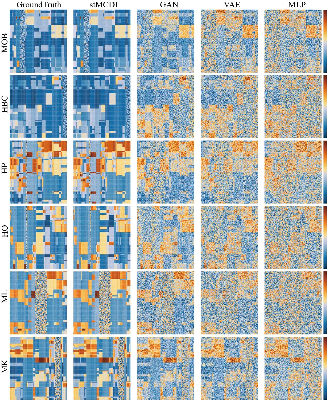
Figure 4: Visualization of the imputation performance of various generative methods across six distinct spatial transcriptomic datasets.

In order to better verify the effectiveness of our proposed method, we also compared stMCDI with several common generative models. To maintain experimental consistency, we still perform diffusion and reduction on the latent representation constructed by the graph encoder. As before, we use the mask part data as the real label, and visualize the prediction part of each model through clustering, as shown in the Fig. 4. We used GAN Yoon et al. [2018], VAE Qiu et al. [2020], and a three-layer MLP. Experimental results show that our proposed method achieves the best performance in the imputation of missing values.

F.2 More results in Basline comparison

Due to the limited length of the text, some baseline comparisons are placed in the supplementary materials, as shown in the Fig. 5.

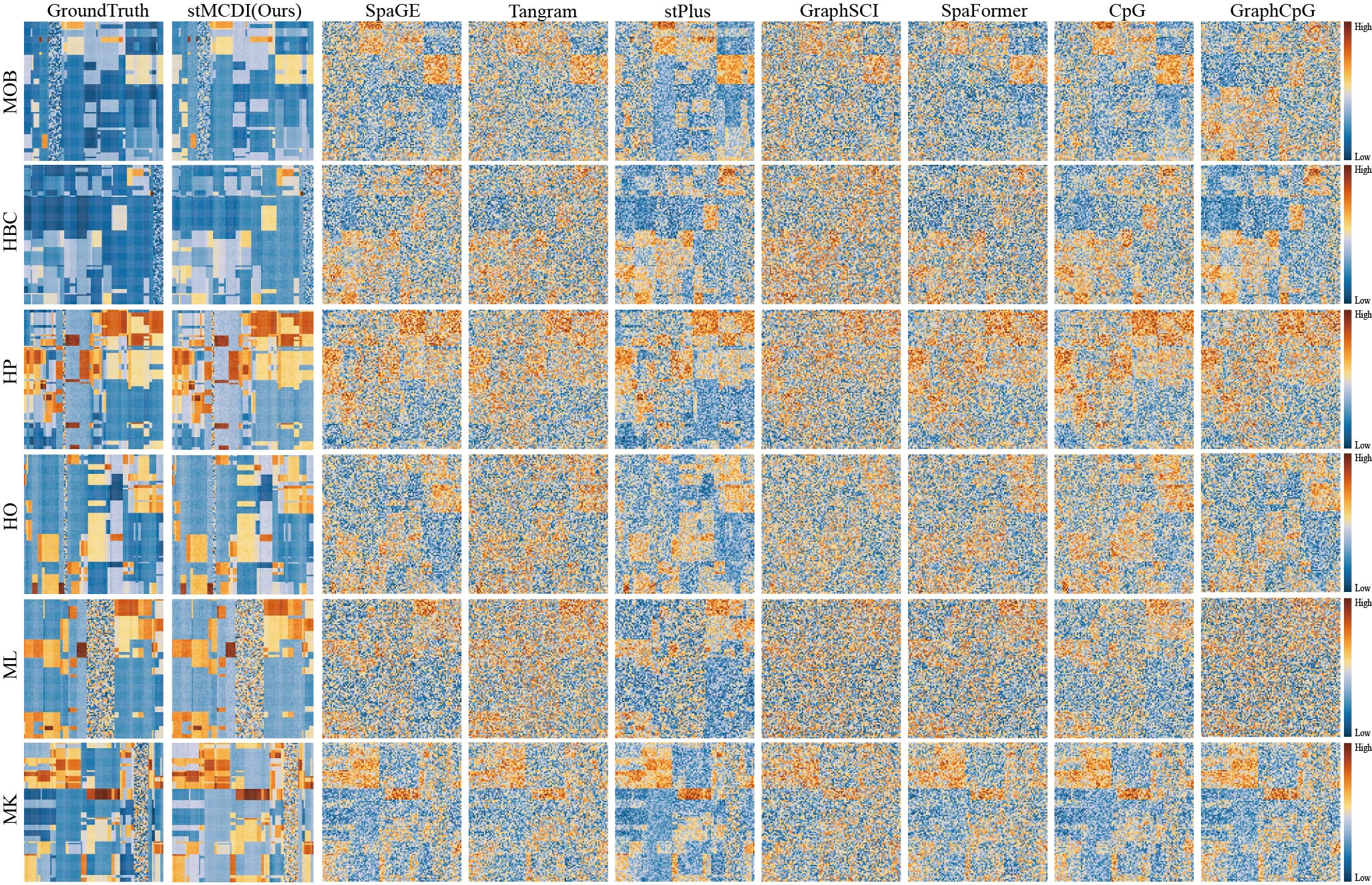
Figure 5: Visualization of the imputation performance of various baseline methods across six distinct spatial transcriptomic datasets.

References

- Abdelaal et al. [2020] Tamim Abdelaal, Soufiane Mourragui, Ahmed Mahfouz, and Marcel JT Reinders. Spage: spatial gene enhancement using scrna-seq. Nucleic acids research, 48(18):e107–e107, 2020.
- Biancalani et al. [2021] Tommaso Biancalani, Gabriele Scalia, Lorenzo Buffoni, Raghav Avasthi, Ziqing Lu, Aman Sanger, Neriman Tokcan, Charles R Vanderburg, Åsa Segerstolpe, Meng Zhang, et al. Deep learning and alignment of spatially resolved single-cell transcriptomes with tangram. Nature Methods, 18(11):1352–1362, 2021.
- Brown et al. [2020] Tom Brown, Benjamin Mann, Nick Ryder, Melanie Subbiah, Jared D Kaplan, Prafulla Dhariwal, Arvind Neelakantan, Pranav Shyam, Girish Sastry, Amanda Askell, et al. Language models are few-shot learners. Advances in neural information processing systems, 33:1877–1901, 2020.
- Buenrostro et al. [2015] Jason D Buenrostro, Beijing Wu, Ulrike M Litzenburger, Dave Ruff, Michael L Gonzales, Michael P Snyder, Howard Y Chang, and William J Greenleaf. Single-cell chromatin accessibility reveals principles of regulatory variation. Nature, 523(7561):486–490, 2015.
- Burgess [2019] Darren J Burgess. Spatial transcriptomics coming of age. Nature Reviews Genetics, 20(6):317–317, 2019.
- De Waele et al. [2022] Gaetan De Waele, Jim Clauwaert, Gerben Menschaert, and Willem Waegeman. Cpg transformer for imputation of single-cell methylomes. Bioinformatics, 38(3):597–603, 2022.
- Deng et al. [2023] Yuzhong Deng, Jianxiong Tang, Jiyang Zhang, Jianxiao Zou, Que Zhu, and Shicai Fan. Graphcpg: imputation of single-cell methylomes based on locus-aware neighboring subgraphs. Bioinformatics, 39(9):btad533, 2023.
- Dong and Zhang [2022] Kangning Dong and Shihua Zhang. Deciphering spatial domains from spatially resolved transcriptomics with an adaptive graph attention auto-encoder. Nature communications, 13(1):1739, 2022.
- Eraslan et al. [2019] Gökcen Eraslan, Lukas M Simon, Maria Mircea, Nikola S Mueller, and Fabian J Theis. Single-cell rna-seq denoising using a deep count autoencoder. Nature communications, 10(1):390, 2019.
- Fang et al. [2023] Shuangsang Fang, Bichao Chen, Yong Zhang, Haixi Sun, Longqi Liu, Shiping Liu, Yuxiang Li, and Xun Xu. Computational approaches and challenges in spatial transcriptomics. Genomics, Proteomics and Bioinformatics, 21(1):24–47, 2023.
- Figueroa-García et al. [2023] Juan Carlos Figueroa-García, Roman Neruda, and German Hernandez-Pérez. A genetic algorithm for multivariate missing data imputation. Information Sciences, 619:947–967, 2023.
- Fortuin et al. [2020a] Vincent Fortuin, Dmitry Baranchuk, Gunnar Rätsch, and Stephan Mandt. Gp-vae: Deep probabilistic time series imputation. In International conference on artificial intelligence and statistics, pages 1651–1661. PMLR, 2020.
- Fortuin et al. [2020b] Vincent Fortuin, Dmitry Baranchuk, Gunnar Rätsch, and Stephan Mandt. Gp-vae: Deep probabilistic time series imputation. In International conference on artificial intelligence and statistics, pages 1651–1661. PMLR, 2020.
- Gao et al. [2023] Ziqi Gao, Yifan Niu, Jiashun Cheng, Jianheng Tang, Lanqing Li, Tingyang Xu, Peilin Zhao, Fugee Tsung, and Jia Li. Handling missing data via max-entropy regularized graph autoencoder. In Proceedings of the AAAI Conference on Artificial Intelligence, volume 37, pages 7651–7659, 2023.
- He et al. [2022] Kaiming He, Xinlei Chen, Saining Xie, Yanghao Li, Piotr Dollár, and Ross Girshick. Masked autoencoders are scalable vision learners. In Proceedings of the IEEE/CVF conference on computer vision and pattern recognition, pages 16000–16009, 2022.
- Ho et al. [2020] Jonathan Ho, Ajay Jain, and Pieter Abbeel. Denoising diffusion probabilistic models. Advances in neural information processing systems, 33:6840–6851, 2020.
- Hou et al. [2022] Zhenyu Hou, Xiao Liu, Yukuo Cen, Yuxiao Dong, Hongxia Yang, Chunjie Wang, and Jie Tang. Graphmae: Self-supervised masked graph autoencoders. In Proceedings of the 28th ACM SIGKDD Conference on Knowledge Discovery and Data Mining, pages 594–604, 2022.
- Huang et al. [2018] Mo Huang, Jingshu Wang, Eduardo Torre, Hannah Dueck, Sydney Shaffer, Roberto Bonasio, John I Murray, Arjun Raj, Mingyao Li, and Nancy R Zhang. Saver: gene expression recovery for single-cell rna sequencing. Nature methods, 15(7):539–542, 2018.
- Huang et al. [2021] Tao Huang, Songjiang Li, Xu Jia, Huchuan Lu, and Jianzhuang Liu. Neighbor2neighbor: Self-supervised denoising from single noisy images. In Proceedings of the IEEE/CVF conference on computer vision and pattern recognition, pages 14781–14790, 2021.
- Kenton and Toutanova [2019] Jacob Devlin Ming-Wei Chang Kenton and Lee Kristina Toutanova. Bert: Pre-training of deep bidirectional transformers for language understanding. In Proceedings of naacL-HLT, volume 1, page 2, 2019.
- Kong et al. [2020] Zhifeng Kong, Wei Ping, Jiaji Huang, Kexin Zhao, and Bryan Catanzaro. Diffwave: A versatile diffusion model for audio synthesis. arXiv preprint arXiv:2009.09761, 2020.
- Kong et al. [2023] Xiangjie Kong, Wenfeng Zhou, Guojiang Shen, Wenyi Zhang, Nali Liu, and Yao Yang. Dynamic graph convolutional recurrent imputation network for spatiotemporal traffic missing data. Knowledge-Based Systems, 261:110188, 2023.
- Li and Li [2018] Wei Vivian Li and Jingyi Jessica Li. An accurate and robust imputation method scimpute for single-cell rna-seq data. Nature communications, 9(1):997, 2018.
- Li et al. [2022] Bin Li, Wen Zhang, Chuang Guo, Hao Xu, Longfei Li, Minghao Fang, Yinlei Hu, Xinye Zhang, Xinfeng Yao, Meifang Tang, et al. Benchmarking spatial and single-cell transcriptomics integration methods for transcript distribution prediction and cell type deconvolution. Nature methods, 19(6):662–670, 2022.
- Liu et al. [2023] Qiao Liu, Wanwen Zeng, Wei Zhang, Sicheng Wang, Hongyang Chen, Rui Jiang, Mu Zhou, and Shaoting Zhang. Deep generative modeling and clustering of single cell hi-c data. Briefings in Bioinformatics, 24(1):bbac494, 2023.
- Lopez et al. [2019] Romain Lopez, Achille Nazaret, Maxime Langevin, Jules Samaran, Jeffrey Regier, Michael I Jordan, and Nir Yosef. A joint model of unpaired data from scrna-seq and spatial transcriptomics for imputing missing gene expression measurements. arXiv preprint arXiv:1905.02269, 2019.
- Luo et al. [2018] Yonghong Luo, Xiangrui Cai, Ying Zhang, Jun Xu, et al. Multivariate time series imputation with generative adversarial networks. Advances in neural information processing systems, 31, 2018.
- Moses and Pachter [2022] Lambda Moses and Lior Pachter. Museum of spatial transcriptomics. Nature Methods, 19(5):534–546, 2022.
- Nichol and Dhariwal [2021] Alexander Quinn Nichol and Prafulla Dhariwal. Improved denoising diffusion probabilistic models. In International Conference on Machine Learning, pages 8162–8171. PMLR, 2021.
- Qiu et al. [2020] Yeping Lina Qiu, Hong Zheng, and Olivier Gevaert. Genomic data imputation with variational auto-encoders. GigaScience, 9(8):giaa082, 2020.
- Rao et al. [2021] Jiahua Rao, Xiang Zhou, Yutong Lu, Huiying Zhao, and Yuedong Yang. Imputing single-cell rna-seq data by combining graph convolution and autoencoder neural networks. Iscience, 24(5), 2021.
- Shengquan et al. [2021] Chen Shengquan, Zhang Boheng, Chen Xiaoyang, Zhang Xuegong, and Jiang Rui. stplus: a reference-based method for the accurate enhancement of spatial transcriptomics. Bioinformatics, 37(Supplement_1):i299–i307, 2021.
- Sohl-Dickstein et al. [2015] Jascha Sohl-Dickstein, Eric Weiss, Niru Maheswaranathan, and Surya Ganguli. Deep unsupervised learning using nonequilibrium thermodynamics. In International conference on machine learning, pages 2256–2265. PMLR, 2015.
- Song et al. [2020] Jiaming Song, Chenlin Meng, and Stefano Ermon. Denoising diffusion implicit models. arXiv preprint arXiv:2010.02502, 2020.
- Sousa da Mota et al. [2023] Bárbara Sousa da Mota, Simone Rubinacci, Diana Ivette Cruz Dávalos, Carlos Eduardo G. Amorim, Martin Sikora, Niels N Johannsen, Marzena H Szmyt, Piotr Włodarczak, Anita Szczepanek, Marcin M Przybyła, et al. Imputation of ancient human genomes. Nature Communications, 14(1):3660, 2023.
- Sun et al. [2023] Yige Sun, Jing Li, Yifan Xu, Tingting Zhang, and Xiaofeng Wang. Deep learning versus conventional methods for missing data imputation: A review and comparative study. Expert Systems with Applications, page 120201, 2023.
- Talwar et al. [2018] Divyanshu Talwar, Aanchal Mongia, Debarka Sengupta, and Angshul Majumdar. Autoimpute: Autoencoder based imputation of single-cell rna-seq data. Scientific reports, 8(1):16329, 2018.
- Tashiro et al. [2021] Yusuke Tashiro, Jiaming Song, Yang Song, and Stefano Ermon. Csdi: Conditional score-based diffusion models for probabilistic time series imputation. Advances in Neural Information Processing Systems, 34:24804–24816, 2021.
- Telyatnikov and Scardapane [2023] Lev Telyatnikov and Simone Scardapane. Egg-gae: scalable graph neural networks for tabular data imputation. In International Conference on Artificial Intelligence and Statistics, pages 2661–2676. PMLR, 2023.
- Tipirneni and Reddy [2022] Sindhu Tipirneni and Chandan K Reddy. Self-supervised transformer for sparse and irregularly sampled multivariate clinical time-series. ACM Transactions on Knowledge Discovery from Data (TKDD), 16(6):1–17, 2022.
- Wang et al. [2021] Juexin Wang, Anjun Ma, Yuzhou Chang, Jianting Gong, Yuexu Jiang, Ren Qi, Cankun Wang, Hongjun Fu, Qin Ma, and Dong Xu. scgnn is a novel graph neural network framework for single-cell rna-seq analyses. Nature communications, 12(1):1882, 2021.
- Wen et al. [2023] Hongzhi Wen, Wenzhuo Tang, Wei Jin, Jiayuan Ding, Renming Liu, Feng Shi, Yuying Xie, and Jiliang Tang. Single cells are spatial tokens: Transformers for spatial transcriptomic data imputation. arXiv preprint arXiv:2302.03038, 2023.
- Xie et al. [2020] Yaochen Xie, Zhengyang Wang, and Shuiwang Ji. Noise2same: Optimizing a self-supervised bound for image denoising. Advances in neural information processing systems, 33:20320–20330, 2020.
- Yarlagadda et al. [2023] Dig Vijay Kumar Yarlagadda, Joan Massagué, and Christina Leslie. Discrete representation learning for modeling imaging-based spatial transcriptomics data. In Proceedings of the IEEE/CVF International Conference on Computer Vision, pages 3846–3855, 2023.
- Yoon et al. [2018] Jinsung Yoon, James Jordon, and Mihaela Schaar. Gain: Missing data imputation using generative adversarial nets. In International conference on machine learning, pages 5689–5698. PMLR, 2018.