Neural-Kernel Conditional Mean Embeddings

Abstract

Kernel conditional mean embeddings (CMEs) offer a powerful framework for representing conditional distribution, but they often face scalability and expressiveness challenges. In this work, we propose a new method that effectively combines the strengths of deep learning with CMEs in order to address these challenges. Specifically, our approach leverages the end-to-end neural network (NN) optimization framework using a kernel-based objective. This design circumvents the computationally expensive Gram matrix inversion required by current CME methods. To further enhance performance, we provide efficient strategies to optimize the remaining kernel hyperparameters. In conditional density estimation tasks, our NN-CME hybrid achieves competitive performance and often surpasses existing deep learning-based methods. Lastly, we showcase its remarkable versatility by seamlessly integrating it into reinforcement learning (RL) contexts. Building on Q-learning, our approach naturally leads to a new variant of distributional RL methods, which demonstrates consistent effectiveness across different environments.

1 Introduction

When conditional distributions present complexities such as multimodality, skewness, or heteroscedastic noise, simply capturing the conditional mean no longer suffices. Kernel conditional mean embeddings (CMEs) (Song et al., 2009; Muandet et al., 2017) represent conditional distributions as elements within a reproducing kernel Hilbert space (RKHS), a space associated to a positive definite kernel. Given both input and output variables, CMEs map these variables into a high-dimensional (often infinite) feature space using kernels, enabling nonparametric and flexible characterization of conditional distributions. Indeed, CMEs have been successfully employed in settings such as probabilistic inference tasks (Fukumizu et al., 2013; Song et al., 2013) and causal inference tasks (Singh et al., 2019; Muandet et al., 2021; Chau et al., 2021; Park et al., 2021).

However, CMEs possess several limitations. First, Gram matrix inversion, needed for standard CME estimation, can become prohibitively expensive when the dataset grows large. Second, the pre-specified nature of RKHS features can lead to poor performance when dealing with high-dimensional variables exhibiting highly nonlinear structures. Lastly, standard hyperparameter tuning procedures such as cross-validation are not applicable for selecting hyperparameters of the kernel on output variables. This last limitation arises because the objective function is defined in terms of the RKHS norm associated to this kernel, and any change in kernel parameters fundamentally alters the objective function itself.

To address these challenges, we propose a method that effectively blends deep learning with CMEs. The central concept involves replacing computationally demanding matrix inversion with a neural network (NN) model, while simultaneously leveraging the feature learning capabilities of deep learning. Our method integrates seamlessly with standard NN training procedures, differing only in its use of an RKHS-based loss function. Additionally, we propose using a specific type of kernel on the output variable, and introduce supplementary objective functions tailored to optimize the kernel parameters. Notably, we offer two flexible options for the hyperparameter optimization: iterative or joint optimization with the NN training process.

The true potential of CMEs lies in their applicability beyond standard density estimation tasks. Namely, CME representations can be employed to define metrics over the space of conditional probability distributions (Gretton et al., 2012). This powerful property, coupled with the efficient incorporation of NNs within our approach, paves the way for effortless adoption within deep reinforcement learning (RL) contexts. By modeling discounted sum of rewards using our NN-based CME representation, we naturally arrive at a new variant of distributional RL (Bellemare et al., 2017, 2023) methods. Our approach shares traits with two existing methods, CDQN (Bellemare et al., 2017) and MMDQN (Nguyen-Tang et al., 2021), while demonstrating consistent efficacy across three benchmark environments.

The paper is organized as follows: Section 2 introduces kernel mean embeddings and CMEs, including a NN-parameterized deep feature approach. Section 3 presents our NN-CME hybrid approach and two hyperparameter optimization strategies. Section 4 demonstrates the performance of our method on both synthetic and real-world datasets. Section 5 delves into RL, introducing our new distributional RL method and assessing its performance in three classic control environments.

2 Background and Preliminaries

Notations: We consider random variables $X$ and $Y$, residing in domains $\mathcal{X}\subseteq\mathbb{R}^{d_{x}}$ and $\mathcal{Y}\subseteq\mathbb{R}^{d_{y}}$, respectively, with realizations $x$ and $y$, joint distribution $P$, and density function $p(x,y)$. Measurable positive definite kernels $k_{\mathcal{X}}:\mathcal{X}\times\mathcal{X}\to\mathbb{R}$ and $k_{\mathcal{Y}}:\mathcal{Y}\times\mathcal{Y}\to\mathbb{R}$, associated with RKHSs $\mathcal{H}_{\mathcal{X}}$ and $\mathcal{H}_{\mathcal{Y}}$, induce features $\psi(x)=k_{\mathcal{X}}(x,\cdot)$ and $\phi(y)=k_{\mathcal{Y}}(y,\cdot)$. The Inner product is denoted by $\left\langle\cdot,\cdot\right\rangle_{\mathcal{H}}$ and the RKHS norm by $\|\cdot\|_{\mathcal{H}}$.

2.1 Kernel Mean Embeddings

For a given marginal distribution $P(X)$, the kernel mean embedding (KME) $\mu_{P(X)}$ is defined as the expectation of the feature $\psi(X)$:

$$\mu_{P(X)}=\mathbb{E}_{X}\left[\psi(X)\right]\in\mathcal{H}_{\mathcal{X}},$$

and always exists for bounded kernels. The reproducing property of RKHSs equips KMEs with the useful ability to estimate function expectations: $\left\langle f,\mu_{P(X)}\right\rangle_{\mathcal{H}_{\mathcal{X}}}=\mathbb{E}_{X}\left[f(X)\right]$ for any $f\in\mathcal{H}_{\mathcal{X}}$. Furthermore, for characteristic kernels, these embeddings are injective, uniquely defining the probability distribution (Fukumizu et al., 2008; Sriperumbudur et al., 2010). For instance, popular kernels such as Gaussian and Laplace kernels possess this property.

The second order mean embeddings, also known as covariance operators (Fukumizu et al., 2004), are defined as the expectation of tensor products between features, for instance:

$$C_{XY}\!=\!\mathbb{E}_{XY}\left[\psi(X)\!\otimes\!\phi(Y)\right],$$

where $\otimes$ is the tensor product, and always exist for bounded kernels. Covariance operators generalize the familiar notion covariance matrices to accommodate infinite-dimensional feature spaces.

2.2 Kernel Conditional Mean Embeddings

With the aforementioned building blocks in place, we now extend KMEs to to the case of conditional distributions, defining kernel conditional mean embeddings (CMEs) (Song et al., 2009; Muandet et al., 2017) as follows:

$$\mu_{P(Y|X)}(x)=\mathbb{E}_{Y|x}\left[\phi(Y)|X=x\right]\in\mathcal{H}_{\mathcal{Y}},$$

requiring an operator $C_{Y|X}:\mathcal{H}_{\mathcal{X}}\rightarrow\mathcal{H}_{\mathcal{Y}}$ that satisfies: (a) $\mu_{P(Y|X)}(x)=C_{Y|X}\psi(x)$ and (b) $\left\langle g,\mu_{P(Y|X)}(x)\right\rangle_{\mathcal{H}_{\mathcal{Y}}}=\mathbb{E}_{Y|x}\left[g(Y)|X=x\right]$ for $g\in\mathcal{H}_{\mathcal{Y}}$. Assuming $\mathbb{E}_{Y|x}\left[g(Y)|X=\cdot\right]\in\mathcal{H}_{\mathcal{X}}$, the following operator satisfies the requirements:

$$C_{Y|X}=(C_{XX})^{-1}C_{XY}.$$

Given i.i.d samples $\{(x_{i},y_{i})\}_{i=1}^{n}\sim P$, an empirical estimate of the operator can be obtained as follows:

$$\hat{C}_{Y|X} =(\hat{C}_{XX}+\lambda I)^{-1}\hat{C}_{XY}$$

$$=\Phi(K_{X}+\lambda I)^{-1}\Psi^{\top},$$

where $\lambda>0$ is a regularization parameter, $K_{X}$ is the Gram matrix $(K_{X})_{ij}=k_{\mathcal{X}}(x_{i},x_{j})$, and $\Psi$ and $\Phi$ are the feature matrices stacked by columns: $\Psi=[\psi(x_{1}),\dots,\psi(x_{n})]$ and $\Phi=[\phi(y_{1}),\dots,\phi(y_{n})]$. Alternatively, this empirical estimate can be obtained by solving following function-valued regression problem (Grünewälder et al., 2012):

$$\operatorname*{arg\,min}_{C:\mathcal{H}_{\mathcal{X}}\rightarrow\mathcal{H}_{\mathcal{Y}}}\frac{1}{n}\sum_{i=1}^{n}\left\|\phi(y_{i})-C\psi(x_{i})\right\|_{\mathcal{H}_{\mathcal{Y}}}^{2}+\lambda\left\|C\right\|_{HS}^{2},$$ (1)

where $\|C\|_{HS}$ is the Hilbert-Schmidt norm. Putting together these elements, we arrive at the empirical estimator:

$$\hat{\mu}_{P(Y|X)}(x)=\hat{C}\psi(x)=\sum_{i=1}^{n}\beta_{i}(x)\phi(y_{i})=\Phi\bm{\beta}(x),$$ (2)

where:

$$\bm{\beta}(x)=(K_{X}+\lambda I)^{-1}\bm{k}_{X},$$

with $\bm{k}_{X}=[k_{\mathcal{X}}(x_{1},x),\dots,k_{\mathcal{X}}(x_{n},x)]^{\top}$. In contrast to KMEs for marginal distributions, CMEs employ non-uniform weights $\beta_{i}(x)$, which are not constrained to be positive or sum up to one.

2.3 Deep Feature Approach

Instead of relying on pre-specified RKHS feature maps, the Deep Feature approach (DF) (Xu et al., 2021) harnesses the adaptive capabilities of deep learning to learn tailored feature representations. This approach has demonstrated its efficacy in settings such as causal inference (Xu et al., 2021) and kernelized Bayes’ rule (Xu et al., 2022), often outperforming classical CME methods.

By replacing $\psi$ with a $d$-dimensional NN-parameterized feature map $\psi_{\theta}:\mathcal{X}\to\mathbb{R}^{d}$ (where $\theta$ denotes the NN’s parameters) in (1), we can jointly optimize both the feature representation and the conditional operator $C$. This is achieved by optimizing $\theta$ with the following loss function:

$$\hat{\mathcal{L}}(\theta)=\mathrm{tr}\left(K_{Y}(I-\Psi^{\top}_{\theta}(\Psi_{\theta}\Psi_{\theta}^{\top}+\lambda I)^{-1}\Psi_{\theta})\right),$$

where $K_{Y}$ is the Gram matrix with elements $(K_{Y})_{ij}=k_{\mathcal{Y}}(y_{i},y_{j})$, and gradient-based optimization methods can be applied. Given the learned parameter $\hat{\theta}=\operatorname*{arg\,min}_{\theta}\hat{\mathcal{L}}(\theta)$, we can express $\bm{\beta}(x)$ in (2) as follows:

$$\bm{\beta}(x)=\Psi^{\top}_{\hat{\theta}}\left(\Psi_{\hat{\theta}}\Psi^{\top}_{\hat{\theta}}+\lambda I\right)^{-1}\psi_{\hat{\theta}}(x).$$

This DF approach offers a partial solution to scalability challenges as well. Its computational complexity of $O(nd^{2}+d^{3})$ is typically smaller than the $O(n^{3})$ complexity of classical approaches. During the training, mini-batch optimization can be be applied for further acceleration. However, the regularization parameter $\lambda$ plays a vital role in both performance and numerical stability, and its selection often necessitates computationally expensive cross-validation procedures involving multiple NN optimizations. Additionally, this approach on its own does not address the remaining hyperparameter selection issue for $k_{\mathcal{Y}}$.

3 Neural Network Based CME

3.1 Model and Objective Function

While DF approach of Xu et al. (2021) partially addresses computational challenges of CME, it still restricts $\bm{\beta}(x)$ to a specific functional form involving matrix inversion. The core idea of our approach is to replace $\bm{\beta}(x)$ in (2) with $f(x;\theta):\mathcal{X}\to\mathbb{R}^{M}$, a NN parameterized by $\theta$. We propose the CME estimator of the following form:

$$\hat{\mu}_{P(Y|X)}(x)=\sum_{a=1}^{M}\phi(\eta_{a})f_{a}(x;\theta),$$

where $\eta_{a}\in\mathcal{Y}$ are $M$ location parameters. These parameters can be optimized together with the NN parameter $\theta$, or can be fixed to reduce the number of parameters. In this paper, we opt for fixing them throughout for easiness of optimization. Analogous to (1) but without $\|C\|^{2}_{HS}$, $\theta$ is optimized through:

$$\min_{\theta}\frac{1}{n}\sum_{i=1}^{n}\left\|\phi(y_{i})-\sum_{i=1}^{M}\phi(\eta_{a})f_{a}(x_{i};\theta)\right\|_{\mathcal{H}_{\mathcal{Y}}}^{2}.$$

We denote this as $\min_{\theta}\frac{1}{n}\sum_{i=1}^{n}\hat{\ell}(\theta)$, where $\hat{\ell}(\theta)$ can be further expressed as:

$$\hat{\ell}(\theta)=-2\sum_{a}k_{\mathcal{Y}}(y_{i},\eta_{a})w_{a}+\sum_{a,b}k_{\mathcal{Y}}(\eta_{a},\eta_{b})w_{a}w_{b},$$ (3)

with $w_{a}=f_{a}(x_{i};\theta)$ and $w_{b}=f_{b}(x_{i};\theta)$. The term $\sum_{i=1}^{n}k_{\mathcal{Y}}(y_{i},y_{i})$ is omitted, assuming fixed hyperparameters for $k_{\mathcal{Y}}$, for now. In contrast to DF, the whole process of calculating $\bm{\beta}(x)$ with explicit features is effectively amortized with $f(x;\theta)$. This eliminates the need for both Gram matrix inversion and regularization parameter selection.

However, selecting hyperparameters for $k_{\mathcal{Y}}$ remains a challenge due to the dependence of the objective values on the RKHS norm $\|\cdot\|_{\mathcal{H}}$; they are not comparable for different hyperparameters. While downstream tasks can sometimes guide tuning (e.g., in IV regression: Xu et al. (2021)), one typically resorts to heuristic methods like the median heuristic (Gretton et al., 2005). Our aim in the following sections is to construct a criterion that can serve as a supplementary objective function for optimizing the $k_{\mathcal{Y}}$ parameter, offering a more effective approach to its selection.

3.2 Choice of Kernel $k_{\mathcal{Y}}$

Our initial step is to employ a positive definite kernel $k$ that satisfies: $k(\cdot,\cdot)\geq 0$ and $\int k(y,\cdot)dy=1$. Thus, the kernels we consider are both reproducing kernels and smoothing kernels for densities, two often confused, but distinct notions of kernel functions. In the following, we adopt what we call the Gaussian density kernel for $k_{\mathcal{Y}}$:

$$k_{\sigma}(y,y^{\prime})=\left(\frac{1}{\sqrt{2\pi\sigma^{2}}}\right)^{d_{y}}\exp\left(-\frac{\|y-y^{\prime}\|^{2}}{2\sigma^{2}}\right).$$

We will denote the associated RKHS by $\mathcal{H}_{\sigma}$. This type of kernel has seen previous use in Kim & Scott (2012); Hsu & Ramos (2019), and variants corresponding to other kernels, such as Laplace and Student kernels, are also available. Because Gaussian density kernel is also a smoothing kernel, CME estimator also gives an estimator $\hat{p}(y|x)$ of the conditional probability density, obtained through the inner product $\left\langle k_{\sigma}(y,\cdot),\hat{\mu}_{P(Y|X)}(x)\right\rangle_{\mathcal{H}_{\sigma}}$ as

$$\hat{\mathbb{E}}_{Y|x}[k_{\sigma}(y,Y)|X=x]=\sum_{a=1}^{M}k_{\sigma}(y,\eta_{a})f_{a}(x;\theta).$$ (4)

This form of density estimate has been theoretically discussed in Kanagawa & Fukumizu (2014). It is also worth noting that with similar probability estimate, Hsu & Ramos (2019) constructed a marginal likelihood-like objective for hyperparameter selection of CMEs, within the context of likelihood-free inference. While they prove that this objective provides an asymptotically correct likelihood surrogate, it is not guaranteed to be positive or normalized for finite data. Consequently, we treat it solely as a proxy for conditional probability, limiting its use to hyperparameter selection criteria.

We emphasize that our focus is on CMEs, i.e. on representing conditional distributions as mean elements within the RKHS. This enables two key advantages: first, we can represent distributions even without constraining the NN output, and second, it opens up applications beyond standard density estimation tasks, as showcased by the unique properties of KMEs explored in Section 5.

3.2.1 Approach 1: Iterative Optimization

Based on the conditional probability estimate (4), we propose optimizing the bandwidth parameter $\sigma$ to minimize an objective function based on $L^{2}$ norm. Accordingly, we adopt the following squared (SQ) error loss:

$$\mathcal{L}_{SQ}=\frac{1}{2}\iint\left(\hat{p}(y|x)-p(y|x)\right)^{2}p(x)dxdy.$$

This objective function has been used in the density-ratio-based conditional density estimation method (Sugiyama et al., 2010). In our case, by plugging in $\hat{p}(y|x)=\sum_{a=1}^{M}k_{\sigma}(y,\eta_{a})f_{a}(x;\theta)$, we obtain the following empirical loss $\frac{1}{n}\sum_{i=1}^{n}\hat{\ell}_{SQ}(\sigma)$, where:

$$\hat{\ell}_{SQ}(\sigma)=-2\sum_{a}k_{\sigma}(y_{i},\eta_{a})w_{a}+\sum_{a,b}k_{\sqrt{2}\sigma}(\eta_{a},\eta_{b})w_{a}w_{b}.$$

The derivation is given in Appendix A. In practice, we iteratively optimize $\theta$ and $\sigma$, through $\min_{\theta}\frac{1}{n}\sum_{i=1}^{n}\hat{\ell}(\theta)$ and $\min_{\sigma}\frac{1}{n}\sum_{i=1}^{n}\hat{\ell}_{SQ}(\sigma)$, every step. Since $\eta_{a}$ within $k_{\sigma}(\cdot,\eta_{a})$ are model parameters, and not randomly sampled during optimization, $\sigma$ can be optimized stably using minibatch optimization, with minimal gradient variance. Complemented with regularization techniques such as weight decay (Loshchilov & Hutter, 2019), we observe that the optimization can generally be carried out without encountering severe overfitting.

3.2.2 Approach 2: Joint Optimization

Interestingly, the only distinction between (3) and $\hat{\ell}_{SQ}(\sigma)$ lies in their second terms, representing the squared functional norms on $\mathcal{H}_{\sigma}$ and $\mathcal{H}_{\sqrt{2}\sigma}$, respectively. This close resemblance hints at the potential for joint optimization of $\theta$ and $\sigma$ using the objective function given in (3), expressed as $\min_{\theta,\sigma}\frac{1}{n}\sum_{i=1}^{n}\hat{\ell}(\theta,\sigma)$. The following theorem provides a key justification for this approach by establishing an inequality that connects these two norms:

Theorem 3.1.

Let $f=\sum_{a=1}^{M}k_{\sqrt{2}\sigma}(\cdot,\eta_{a})w_{a}\in\mathcal{H}_{\sqrt{2}\sigma}$ and $g=\sum_{a=1}^{M}k_{\sigma}(\cdot,\eta_{a})w_{a}\in\mathcal{H}_{\sigma}$. Then the following inequality holds:

$$\|f\|_{\mathcal{H}_{\sqrt{2}\sigma}}\leq\|g\|_{\mathcal{H}_{\sigma}}.$$

The proof, provided in Appendix B, leverages the Fourier transform expression of RKHS for translation invariant kernels. By replacing the second term of $\hat{\ell}_{SQ}(\sigma)$ with this upper bound, we observe a coincidence with the original objective function (3). This result validates our proposal for joint optimization of $\theta$ and $\sigma$ using (3), since it simultaneously optimizes an upper bound of $\hat{\ell}_{SQ}(\sigma)$ for $\sigma$, while optimizing the original loss function for $\theta$. Joint optimization not only simplifies the procedure but also, as a valuable byproduct, mitigates overfitting in hyperparameter optimization due to the utilization of an upper bound. Indeed, we observe that joint optimization, with its combined advantages, yields stable performance across various datasets.

3.3 Related Work

Mixture Density Networks (MDNs) (Bishop, 1994) model conditional probability distributions as a mixture of (typically) Gaussian components, where the NN directly predicts means, variances, and mixing weights. Due to their simplicity, MDNs have been used in diverse tasks (Papamakarios & Murray, 2016; Makansi et al., 2019).

Normalizing Flows (NFs) (Rezende & Mohamed, 2015; Papamakarios et al., 2021) transform a simple base distribution using invertible mappings parameterized by NNs, ultimately yielding the desired distribution. Particularly, conditional version of NFs that utilize monotonic rational-quadratic splines for the transformation (Durkan et al., 2019), have found extensive use in simulation-based inference settings (Lueckmann et al., 2021).

Also, Han et al. (2022) recently proposed CARD, a conditional density estimator (and classifier) based on diffusion models. CARD combines a denoising diffusion-based conditional generative model with a pre-trained conditional mean estimator, achieving strong performance in diverse practical settings.

We will compare these methods with our proposed approaches in the following experimental sections.

4 Experiments on Density Estimation

To investigate the effectiveness of our approach, we conduct experiments on both toy and real-world datasets. We focus on conditional density estimation tasks where the dimension of the output variable is one ($d_{y}=1$). Note that the input variable can be multi-dimensional, and we conduct experiments on such settings using UCI datasets (Dua & Graff, 2017), where $d_{x}$ can be up to 90.

We denote our approach proposed in Subsections 3.2.1 and 3.2.2 as Proposal-Iterative and Proposal-Joint, respectively. We compare with DF, MDN, NF, and CARD. For DF, we tested two models: DF used with the median heuristic for bandwidth selection (DF-med) and DF with bandwidth fixed to 0.1 (DF-0.1). For NF, we use the conditional version of autoregressive Neural Spline Flow (Durkan et al., 2019).

Both evaluation metrics employed in these settings require samples from the learned model. To sample points from CME-based approaches, we employ kernel herding (Chen et al., 2010), a deterministic sampling method that yields super-samples.

Table 1: WAS1 for toy datasets. Values are multiplied by $100$.

Dataset			WAS1 $\downarrow$
	Proposal-Iterative	Proposal-Joint	DF-med	DF-0.1	MDN	NF	CARD
Bimodal	$5.88\pm 0.28$	$\bm{5.67\pm 0.28}$	$10.87\pm 0.23$	$5.93\pm 0.23$	$6.23\pm 0.27$	$6.83\pm 0.50$	$6.59\pm 0.46$
Skewed	$4.86\pm 0.23$	$\bm{4.68\pm 0.22}$	$6.07\pm 0.19$	$5.26\pm 0.19$	$5.76\pm 0.18$	$6.56\pm 0.29$	$5.93\pm 0.26$
Ring	$\bm{21.13\pm 0.99}$	$\bm{21.10\pm 1.14}$	$26.17\pm 1.16$	$22.16\pm 1.25$	$26.66\pm 0.80$	$27.99\pm 1.74$	$29.91\pm 0.97$

Table 2: QICE (in ${\%}$) for UCI datasets.

Dataset			QICE $\downarrow$
	Proposal-Iterative	Proposal-Joint	DF-med	DF-0.1	MDN	NF	CARD
Boston	$\bm{3.15\pm 0.92}$	$\bm{3.09\pm 0.53}$	$5.74\pm 1.17$	$3.88\pm 0.82$	$4.85\pm 1.19$	$4.09\pm 0.95$	$3.45\pm 0.83$
Concrete	$3.06\pm 0.82$	$3.21\pm 0.72$	$4.05\pm 0.95$	$4.11\pm 0.66$	$3.21\pm 0.79$	$2.90\pm 0.79$	$\bm{2.30\pm 0.66}$
Energy	$\bm{2.89\pm 0.69}$	$3.29\pm 0.73$	$7.14\pm 0.88$	$3.23\pm 0.90$	$3.54\pm 0.85$	$3.62\pm 1.23$	$4.91\pm 0.94$
Kin8nm	$0.98\pm 0.29$	$\bm{0.91\pm 0.19}$	$4.70\pm 0.32$	$2.60\pm 0.41$	$2.42\pm 0.32$	$1.75\pm 0.87$	$\bm{0.92\pm 0.25}$
Naval	$10.88\pm 1.09$	$6.81\pm 1.07$	$7.09\pm 1.04$	$8.71\pm 0.37$	$8.34\pm 3.41$	$4.41\pm 1.54$	$\bm{0.80\pm 0.21}$
Power	$0.88\pm 0.24$	$\bm{0.84\pm 0.18}$	$4.81\pm 0.33$	$2.91\pm 0.18$	$1.34\pm 0.35$	$1.35\pm 0.59$	$0.92\pm 0.21$
Protein	$\bm{0.48\pm 0.05}$	$0.55\pm 0.17$	$1.83\pm 0.19$	$0.80\pm 0.07$	$1.09\pm 0.35$	$0.80\pm 0.38$	$0.71\pm 0.11$
Year	$0.71\pm$ NA	$\bm{0.53\pm}$ NA	$1.80\pm$ NA	$0.56\pm$ NA	$0.74\pm$ NA	$1.02\pm$ NA	$\bm{0.53\pm}$ NA

4.1 Toy Data

Set Up:

We conduct experiments on three distinct toy datasets: Bimodal, Skewed, and Ring. Each dataset features a one-dimensional input variable and comprises 5000 data points for training.

These datasets are designed to challenge models with diverse distributional characteristics: Bimodal dataset comprised of two Gaussian distributions, but the degree of bimodality and noise levels vary depending on the value of $x$. Skewed dataset are sampled from a skew-normal distribution, but distribution parameters, such as skewness, change as a function of $x$. Ring dataset features a ring-shaped distribution with an embedded box-shaped distribution. The detailed generation process as well as a figure for each dataset is provided in Appendix C.

Evaluation Metric:

We evaluate models using a metric based on the Wasserstein-1 distance (WAS1), defined by

$$W_{1}(\mu,\nu)=\inf_{\pi\in\Gamma(\mu,\nu)}\int_{\mathbb{R}\times\mathbb{R}}|x-y|d\pi(x,y),$$

where $\Gamma(\mu,\nu)$ is the set of probability distributions whose marginals are $\mu$ and $\nu$. In the one-dimensional case, this metric can be readily calculated using packages like SciPy (Virtanen et al., 2020).

The evaluation process involves the following steps: we first draw 50 samples from the learned models for each 200 equally spaced evaluation points $x_{\text{test}}$. We then, compute the WAS1s between these samples and 50 points sampled from the true generating process (for each $x_{\text{test}}$). We average the WAS1 values for all evaluation points and report the mean and standard deviation across 10 independent runs.

Results:

The overall results are presented in Table 1, demonstrating that our proposed approaches outperform competitors including NF and CARD. Crucially for DF, the median heuristic fails to achieve optimal performance. It only becomes competitive with our approaches when the parameter is set to 0.1, which was identified through empirical trials. This highlights the general challenge of hyperparameter selection for the output variable kernel in CME-based methods, where both our iterative and joint approaches demonstrably lead to more effective parameter selection.

4.2 UCI Datasets

Set Up:

To further investigate our approaches, we conduct experiments on 8 real-world regression benchmark datasets from the UCI repository. Details of the datasets are provided in Appendix D.

We follow experimental protocols of Han et al. (2022): (a) we employ the same train-test splits with a $90\%/10\%$ ratio, and use 20 folds for all datasets except Protein (5 folds) and Year (1 fold), (b) we standardize both input and output variables for training and remove standardization for evaluation, and (c) for each test data point $x_{\text{test}}$, we sample 1000 points from learned models, conditioned on $x_{\text{test}}$, and calculate the metric described below.

Evaluation Metric:

Since UCI datasets do not have “true generating process”, we adopt the Quantile Interval Coverage Error (QICE) metric proposed also by Han et al. (2022). To compute QICE, we first generate sufficient number of samples for each conditional values $x_{i}$. We then divide the generated samples into $L$ equally spaced bins, resulting in $L$ quantile intervals with boundaries denoted as $\hat{y}_{i}^{\text{low}_{j}}$ and $\hat{y}_{i}^{\text{high}_{j}}$. Then compute the following quantity:

$$\text{QICE}\coloneqq\frac{1}{L}\sum_{j=1}^{L}\bigg{|}r_{j}-\frac{1}{L}\bigg{|},\text{ where }$$

$$r_{j}=\frac{1}{n}\sum_{i=1}^{n}{1}_{y_{i}\geq\hat{y}_{i}^{\text{low}_{j}}}\cdot{1}_{y_{i}\leq\hat{y}_{i}^{\text{high}_{j}}}.$$

When the learned conditional distribution perfectly matches the true distribution, we expect approximately $1/L$ of the true data to fall within each of the $L$ quantile intervals, resulting in a QICE value of 0. In this experiment, we follow Han et al. (2022) and set $L=10$. We report mean and standard deviation of the QICE metric across all splits.

Results:

The overall results are presented in Table 2. It can be seen that our proposed approaches frequently outperform existing methods such as DF, MDN, and NF, and often prove competitive with CARD in terms of the QICE metric. This is particularly impressive considering CARD requires two separate NN optimization procedures: 1. Conditional mean estimator optimization, and 2. Denoising diffusion model optimization, guided by the optimized conditional mean estimator. In contrast, our approaches achieve a comparable level of high-quality density estimation as diffusion-based CARD, while only using a single NN. The Proposal-Joint approach stands out with its exceptional efficiency, requiring only a standard NN training procedure.

It is also worth noting that in the UCI experiments, DF-0.1 clearly underperforms compared to our approaches, crucially demonstrating the importance of tailoring bandwidth $\sigma$ to each dataset for optimal performance. This suggests that a fixed $\sigma$ value, as used in DF-0.1, is typically insufficient for achieving good results across diverse datasets.

5 Applications to Reinforcement Learning

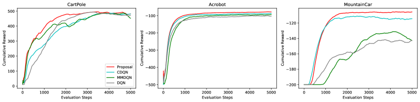
Figure 1: Performance comparison on three environments. We report the mean of cumulative rewards across 10 independent runs.

5.1 Backgrounds

We consider a classical setting in RL, where the framework of a Markov Decision Process (MDP) (Puterman, 2014) governs the agent-environment interactions. MDP is defined by the tuple $(\mathcal{S},\mathcal{A},R,P,\gamma)$, where $\mathcal{S}$ denotes the state space, $\mathcal{A}$ the action space, $P(\cdot|s,a)$ the transition probabilities, $R(s,a)$ the reward dependent on the state and action, and $\gamma\in\left(0,1\right]$ the discount factor. We represent the discounted sum of rewards received by an agent under a policy $\pi$ as a random variable $Z^{\pi}(s,a)=\sum_{t=0}^{\infty}\gamma^{t}R(s_{t},a_{t})$ on space $\mathcal{Z}$, where $s_{0}=s$, $a_{0}=a$, $s_{t+1}\sim P(\cdot|s_{t},a_{t})$, and $a_{t}\sim\pi(\cdot|s_{t})$.

The state-action value, also known as Q-value, is defined as $Q^{\pi}(s,a)=\mathbb{E}\left[Z^{\pi}(s,a)\right]$. In Q-learning (Watkins & Dayan, 1992), the goal is to learn the optimal Q-value, $Q^{\star}(s,a)=\max_{\pi}Q^{\pi}(s,a)$, which is the fixed point of the Bellman optimality operator $\mathcal{T}$:

$$(\mathcal{T}Q)(s,a)\equiv\mathbb{E}\left[R(s,a)\right]+\gamma\mathbb{E}_{P}\left[\max_{a^{\prime}}Q(s^{\prime},a^{\prime})\right],$$

with $s^{\prime}\sim P(\cdot|s,a)$. Deep Q-Network (DQN) (Mnih et al., 2015) represents Q-values with NNs, parameterized by $\theta$, and optimizes them based on the following loss function:

$$\hat{\ell}(\theta)=\left(r+\gamma\max_{a^{\prime}}Q_{\theta^{-}}(s^{\prime},a^{\prime})-Q_{\theta}(s,a)\right)^{2},$$

where $\theta^{-}$ corresponds to the fixed target network, periodically copied from and synchronized with $Q_{\theta}$. A large replay buffer stores experienced transitions $(s,a,r,s^{\prime})$, and batches are sampled for mini-batch optimization, consistent with standard NN training practice.

Instead of only learning the expectation of $Z(s,a)$, distributional RL (DRL) (Bellemare et al., 2017, 2023) aims to approximate its entire distribution. Accordingly, distributional Bellman optimality operator can be defined:

$$(\mathcal{T}Z)(s,a)\overset{D}{\equiv}R(s,a)+\gamma Z\left(s^{\prime},\operatorname*{arg\,max}_{a^{\prime}}\mathbb{E}_{P}\left[Z(s^{\prime},a^{\prime})\right]\right)$$

where, $X\overset{D}{\equiv}Y$ indicates that random variables $X$ and $Y$ follow the same distribution.

Several DRL approaches have significantly advanced the field of RL, achieving performance gains beyond standard DQN. One such approach, Categorical DQN (CDQN) (Bellemare et al., 2017), models distributions as categorical distribution represented by $\sum_{a=1}^{M}\theta_{a}\delta_{a}$, where $\theta_{a}$ are learnable parameters and $\delta_{a}$ represent fixed discrete atoms on a pre-defined grid. Alternatively, some approaches utilize quantile regression for distribution modeling (Dabney et al., 2018). More recently, Nguyen-Tang et al. (2021) proposed Moment Matching DQN (MMDQN), which represents distributions in RKHS. While Nguyen-Tang et al. (2021) did not explicitly formulate their approach based on CMEs, their formulation can be interpreted as a CME variant with uniform weights. We compare and contrast these approaches with our proposed method in Section 5.4.

5.2 Proposed Model for DRL

We propose modeling the (conditional) distribution of $Z(s,a)$ using our NN-CME hybrid approach. This approach leverages a kernel $k_{\mathcal{Z}}(\cdot,z)\in\mathcal{H}_{\mathcal{Z}}$ and represents distributions as:

$$\mu_{P(Z|S,A)}(x)=\sum_{a=1}^{M}k_{\mathcal{Z}}(\cdot,\eta_{a})f_{a}(x;\theta),$$

where $x$ is a tuple of state and action. Here, $\eta_{a}$ are chosen analogously to atoms $\delta_{a}$ in CDQN, effectively covering anticipated support of the distribution. Importantly, our CME parameterization excels by bypassing the need for matrix inversion, enabling efficient action selection. In contrast, applying existing CME approaches (such as DF) in this setting would necessitate evaluating $\bm{\beta}(x)$ in (2) by accessing the entire replay buffer and performing matrix inversion on this data. This can be prohibitively expensive, especially when performed repeatedly.

To construct a loss function in the context of deep Q-learning, we define a metric between the distribution of $R(s,a)+\gamma Z\left(s^{\prime},a^{\prime}\right)$ and that of $Z(s,a)$. Maximum Mean Discrepancy (MMD) (Gretton et al., 2012) provides a principled way to measure the discrepancy between these distributions in the RKHS:

$$\hat{d}_{k_{\mathcal{Z}}}=\left\|\sum_{a=1}^{M}k_{\mathcal{Z}}(\cdot,\tau_{a})v_{a}-\sum_{a=1}^{M}k_{\mathcal{Z}}(\cdot,\eta_{a})w_{a}\right\|_{\mathcal{H}_{\mathcal{Z}}},$$

where $\tau_{a}=r+\gamma\eta_{a}$ and $v_{a}=f_{a}(x;\theta^{-})$. Squaring this MMD leads to our DRL-specific loss function $\hat{d}_{k_{\mathcal{Z}}}^{2}(\theta)$:

$$\hat{d}^{2}_{k_{\mathcal{Z}}}(\theta) =\sum_{a,b}k_{\mathcal{Z}}(\tau_{a},\tau_{b})v_{a}v_{b}-2\sum_{a,b}k_{\mathcal{Z}}(\tau_{a},\eta_{b})v_{a}w_{b}$$

$$+\sum_{a,b}k_{\mathcal{Z}}(\eta_{a},\eta_{b})w_{a}w_{b}.$$

Thus, we have retained the CME parametrization from Section 3, but crucially adopted an MMD-based loss function to suit RL tasks. This flexible adaptation is enabled by both representing distributions as mean elements in the RKHS and exploiting the unique property of KMEs.

5.3 Fusing Kernels

Selecting the hyperparameters for $k_{\mathcal{Z}}$ is an important issue, also in RL settings. Corollary 4.1 of Killingberg & Langseth (2023) implies that careful selection of the bandwidth parameter is crucial for ensuring theoretical convergence in moment matching-based DRL, when used with the Gaussian kernel. Inspired by MMD-FUSE (Biggs et al., 2023), an MMD-based two-sample testing approach, we propose using a distribution over kernels, $k\in\mathcal{K}$. Our approach employs the following log-sum-exp type loss function:

$$\text{FUSE}=\log\left(\mathbb{E}_{k\sim\omega}\left[\exp({\hat{d}^{2}_{k_{\mathcal{Z}}}(\theta)})\right]\right)$$

where $\omega$ is an element of $\mathcal{M}(\mathcal{K})$, the set of distributions over the kernels. For instance, we can define $\omega$ as a uniform distribution over collections of Gaussian kernels with various bandwidths $\sigma>0$, where $\sigma$ are chosen from a uniformly discretized interval. The Donsker-Varadhan equality (Donsker & Varadhan, 1975), as stated in Biggs et al. (2023), offers the following interpretation: $\text{FUSE}=\sup_{\rho}\mathbb{E}_{k\sim\rho}\left[\hat{d}_{k}(\theta)\right]-\text{KL}[\rho\|\omega]$, where KL denotes the Kullback-Leibler divergence, $\rho\in\mathcal{M}(\mathcal{K})$ can be loosely interpreted as the “posterior” over kernels, and $\omega$ as a “prior”. While a theoretical analysis of this approach within the DRL context remains important future work, empirical results suggest its performance advantages compared to using a single fixed kernel.

5.4 Discussions

Both our approach and MMDQN utilize CMEs to model the distributions of $Z(s,a)$. However, they differ in what their NNs parameterize. MMDQN directly learns atoms through its network and assigns them uniform weights, resulting in the representation: $\mu_{P(Z|S,A)}(x)=\frac{1}{M}\sum_{a=1}^{M}k_{\mathcal{Z}}(g_{a}(x;\theta),\cdot)$. While this eliminates the need for manual atom specification, its reliance on uniform weights might hinder its ability to accurately model complex distributions exhibiting multimodality or skewness.

When the predefined atoms $\eta_{a}$ in our approach coincide with the fixed atoms $\delta_{a}$ in CDQN, the parameterizations closely resemble each other. However, a key difference arises in the loss functions: CDQN employs cross-entropy loss, treating the distribution as categorical, whereas we leverage an MMD-based loss function. In essence, while our CME-based representation and MMD-based loss share similarities with MMDQN, our approach aligns more closely with CDQN in its atom structure and NN parameterization, but employs a distinct loss function.

5.5 Experimental Results

Set Up:

To investigate the unique aspects of our method and gain insights into DRL design choices, we tested it on three classic control environments from Gymnasium (Towers et al., 2023): CartPole, Acrobot, and MountainCar. While our approach does not inherently constrain the output of $f(x;\theta)$ to be positive or sum to one, we applied a softmax function in the last layer, analogous to CDQN, making the NN architecture identical to that of CDQN.

We note that while DRL algorithms are often evaluated on complex Atari2600 games, such experiments require extensive computational resources. For instance, the work by Obando-Ceron & Castro (2021) required approximately 5 days to run each agent on each Atari environment using a GPU. As Obando-Ceron & Castro (2021) demonstrated through comprehensive benchmark evaluations, valuable scientific insights can still be drawn from smaller-scale environments. Therefore, our focus in this experiment is on understanding how different parameterizations and loss functions impact various aspects of learning and control effectiveness.

Results:

Figure 1 presents the overall results, demonstrating the consistent effectiveness of our approach across three environments. In CartPole, all methods achieve near-optimal performance, attaining approximately 500 cumulative reward. However, our method demonstrates faster and more stable convergence. In Acrobot, while all methods exhibit stability, ours achieves the highest cumulative reward. On MountainCar, our approach clearly outperforms the others.

Importantly, despite identical distribution parameterization to CDQN, our approach consistently achieves superior performance. This suggests that the MMD-based loss function combined with our fusion strategy contributes to the improved performance. Investigating theoretical justification for this improvement may present a potentially fruitful research direction.

Despite improved performance reported by Nguyen-Tang et al. (2021) on Atari tasks, MMDQN displayed instability in classic control environments. We hypothesize that this disparity arises from the inherent differences in reward structures. Sparse rewards in Atari environments potentially favor MMDQN’s direct particle placement learning, while predetermined atom structure might be more effective in classic control environments with denser rewards. This suggests that the choice of distribution parameterization may depend on the reward structure of environments, highlighting the influence of inductive bias.

6 Conclusion

This paper introduced a new NN-CME hybrid that effectively addresses the key challenges of existing CME methods in terms of scalability, expressiveness, and hyperparameter selection. We proposed to replace the Gram matrix inversion needed for CME estimation with an expressive NN, and presented strategies for optimizing the hyperparameter of $k_{y}$ by leveraging the Gaussian density kernel. We demonstrated its effectiveness in representing conditional distributions: in density estimation tasks, it achieves competitive results, and in RL applications, the proposed method outperforms competing approaches in terms of cumulative reward.

Our approach seamlessly lends itself to diverse other settings, including causal inference tasks where using CMEs offers distinct advantages (Singh et al., 2019; Muandet et al., 2021; Chau et al., 2021; Park et al., 2021). Furthermore, while our approach effectively handled one-dimensional outputs, verifying the effectiveness with more challenging multidimensional settings presents an important area for future investigation. Drawing inspiration from inducing points approaches in Gaussian Process literature (Hensman et al., 2013), optimizing the location parameters $\eta_{a}$ could prove key to achieving effective performance in these broader landscapes.

Impact Statements

This paper makes a contribution to general purpose machine learning methodology, by improving the practicability of models for representing conditional distributions. Such models have a broad applicability and a potential for impact as they are important ingredients in a wide range of learning tasks. When applying the proposed methodology, it is crucial to consider its potential limitations. For instance, our approach, similar to existing density estimation methods, does not readily capture inherent causal relationships between input and output variables, which could be critical for informed decision-making. We encourage practitioners to consider these limitations and use our approach carefully for making reliable decisions in relevant scenarios.

Appendix A Derivation of the Empirical SQ Loss

The SQ loss can be further expanded as follows:

$$\mathcal{L}_{SQ} =\frac{1}{2}\iint\left(\hat{p}(y|x)-p(y|x)\right)^{2}p(x)dxdy.$$

$$=\frac{1}{2}\iint(\hat{p}(y|x))^{2}p(x)dxdy-\iint\hat{p}(y|x)p(x,y)dxdy+C,$$

where $C$ is the constant term. By plugging in $\hat{p}(y|x)=\sum_{a=1}^{M}k_{\sigma}(y,\eta_{a})f_{a}(x;\theta)$, the empirical estimate can be written as:

$$\hat{\mathcal{L}}_{SQ}=\frac{1}{2}\sum_{i}\sum_{a,b}\left(\int k_{\sigma}(\eta_{a},y)k_{\sigma}(y,\eta_{b})dy\right)f_{a}(x_{i};\theta)f_{b}(x_{i};\theta)-\sum_{i}\sum_{a}k_{\sigma}(y_{i},\eta_{a})f_{a}(x_{i};\theta).$$

The second term corresponds to the first term in $\hat{\ell}_{SQ}(\sigma)$. For the first term, we have an integral $\int k_{\sigma}(\eta_{a},y)k_{\sigma}(y,\eta_{b})dy$. With $k_{\sigma}$ having the form of Gaussian density, this can be calculated analytically:

$$\int k(\eta_{a},y)k(y,\eta_{b})dy =\left(\frac{1}{2\pi\sigma^{2}}\right)^{d_{y}}\int\exp\left(-\frac{1}{2\sigma^{2}}(|\eta_{a}-y|^{2}+|y-\eta_{b}|^{2})\right)dy$$

$$=\left(\frac{1}{2\pi\sigma^{2}}\right)^{d_{y}}\int\exp\left(-\frac{1}{4\sigma^{2}}\left(4\left|y-\frac{\eta_{a}+\eta_{b}}{2}\right|^{2}+|\eta_{a}-\eta_{b}|^{2}\right)\right)dy$$

$$=\left(\frac{1}{2\pi\sigma^{2}}\right)^{d_{y}}\int\exp\left(-\frac{1}{\sigma^{2}}\left|y-\frac{\eta_{a}+\eta_{b}}{2}\right|^{2}\right)dy\exp\left(-\frac{1}{4\sigma^{2}}|\eta_{a}-\eta_{b}|^{2}\right)$$

$$=\left(\frac{1}{2\pi(\sqrt{2}\sigma)^{2}}\right)^{d_{y}}\exp\left(-\frac{|\eta_{a}-\eta_{b}|^{2}}{2(\sqrt{2}\sigma)^{2}}\right)$$

$$=k_{\sqrt{2}\sigma}(\eta_{a},\eta_{b}).$$

combining these elements, we obtain:

$$\hat{\mathcal{L}}_{SQ}=\sum_{i=1}^{n}\left(-2\sum_{a}k_{\sigma}(y_{i},\eta_{a})f_{a}(x_{i};\theta)+\sum_{a,b}k_{\sqrt{2}\sigma}(\eta_{a},\eta_{b})f_{a}(x_{i};\theta)f_{b}(x_{i};\theta)\right).$$

Appendix B Proof of Theorem 3.1

We first introduce the Fourier expression of RKHS given by a shift invariant integrable kernel $k(x-y)$ on ${\rm I\!R}^{d}$. Let $\hat{k}$ denote the Fourier transform of $k(z)$:

$$\hat{k}(\omega)=\frac{1}{(2\pi)^{d/2}}\int k(z)e^{-\sqrt{-1}\omega^{T}z}dz.$$

It is known (e.g. Girosi et al., 1995; Saitoh, 1997) that a function $g$ on ${\rm I\!R}^{d}$ is in the corresponding RKHS $\mathcal{H}_{k}$ if and only if

$$\int\frac{|\hat{g}(\omega)|^{2}}{\hat{k}(\omega)}d\omega<\infty$$

and its squared RKHS norm is given by

$$\|g\|_{\mathcal{H}_{k}}^{2}=\int\frac{|\hat{g}(\omega)|^{2}}{\hat{k}(\omega)}d\omega.$$

Note that by Bochner’s theorem, the Fourier transform $\hat{k}(\omega)$ takes non-negative values.

It is well known that, the Fourier transform of Gaussian density kernel $k_{\sigma}(z)=\frac{1}{(2\pi\sigma^{2})^{d/2}}\exp(-\frac{\|z\|^{2}}{2\sigma^{2}})$ is given by

$$\hat{k}_{\sigma}(\omega)=\frac{1}{(2\pi)^{d/2}}e^{-\frac{\sigma^{2}\|\omega\|^{2}}{2}}.$$ (5)

Let

$$g=\sum_{a=1}^{M}k_{\sigma}(\cdot,\eta_{a})w_{a}\in\mathcal{H}_{\sigma}\quad\text{and}\quad f=\sum_{a=1}^{M}k_{\sqrt{2}\sigma}(\cdot,\eta_{a})w_{a}\in\mathcal{H}_{\sqrt{2}\sigma}$$

be the two functions in Theorem 3.1. It is easy to see from the general Fourier formulas that

$$\hat{g}(\omega)=\sum_{a}w_{a}e^{-\sqrt{-1}\eta_{a}^{T}\omega}\hat{k}_{\sigma}(\omega)$$

and thus we obtain from (5)

$$\|g\|_{\mathcal{H}_{\sigma}}^{2}=\frac{1}{(2\pi)^{d/2}}\int\Bigl{|}\sum_{a}w_{a}e^{-\sqrt{-1}\eta_{a}^{T}\omega}\Bigr{|}^{2}\exp\Bigl{(}-\frac{\sigma^{2}\|\omega\|^{2}}{2}\Bigr{)}d\omega.$$

Similarly, by replacing $\sigma$ with $\sqrt{2}\sigma$, we have

$$\|f\|_{\mathcal{H}_{\sqrt{2}\sigma}}^{2}=\frac{1}{(2\pi)^{d/2}}\int\Bigl{|}\sum_{a}w_{a}e^{-\sqrt{-1}\eta_{a}^{T}\omega}\Bigr{|}^{2}\exp\bigl{(}-\sigma^{2}\|\omega\|^{2}\bigr{)}d\omega.$$

It follows from $\exp\bigl{(}-\sigma^{2}\|\omega\|^{2}\bigr{)}\leq\exp\Bigl{(}-\frac{\sigma^{2}\|\omega\|^{2}}{2}\Bigr{)}$ for any $\omega$ that

$$\|f\|_{\mathcal{H}_{\sqrt{2}\sigma}}^{2}\leq\|g\|_{\mathcal{H}_{\sigma}}^{2},$$

which completes the proof.

Appendix C Details on Experiments in Section 4.1

C.1 Data Generating Process

The visualization of the toy datasets used in the experiment is shown in Figure 2. The generating process is provided in the following:

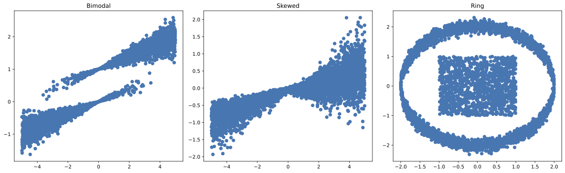
Figure 2: Visualization of toy datasets

Bimodal:

$y=0.2x+P+\epsilon$, where $x\sim U(-5,5)$, $P\sim Binomial\left(\frac{1}{1+\exp(-1.5x)}\right)$, and $\epsilon\sim N(0,(0.05x)^{2})$.

Skewed:

$y\sim SkewNormal(\xi(x),\omega(x),\alpha(x))$, where $x\sim U(-5,5)$, $\xi(x)=0.1x$, $\omega(x)=0.1|x|+0.05$, and $\alpha(x)=-8+8\cdot\left(\frac{1}{1+\exp(-x)}\right)$. Here, $\xi(x)$ corresponds to location, $\omega(x)$ to scale, and $\alpha(x)$ to skewness.

Ring:

$$y=\begin{cases}\begin{cases}U(-1,1)&P_{1}=1/2\\ Ring(x)&P_{1}=1/2\end{cases}&|x|\leq 1\\ Ring(x)&|x|>1\end{cases},$$

and

$$Ring(x)=\begin{cases}2\cdot\sin(\arccos(x/2))+\epsilon&P_{2}=1/2\\ 2\cdot\sin(-\arccos(x/2))+\epsilon&P_{2}=1/2\end{cases},$$

where $x\sim U(-2,2)$ and $\epsilon\sim N(0,0.1^{2})$.

C.2 Architecture and Hyperparameter Choices

We used NNs with two fully-connected hidden layers, each containing 50 ReLU activation units. For the optimizer, we used AdamW (Loshchilov & Hutter, 2019). Other architectural and hyperparameter choices for each model are provided below:

Proposals: We set the number of location points $M=100$, and $\eta_{a}$ were chosen as uniformly spaced grid points within the closed interval bounded by the minimum and maximum values observed in the training data. The learning rate was set to 1e-4, the batch size was set to 50, and the number of training epochs was set to 1000, and $\sigma$ was initialize to 1.0. For Proposals, we have a final layer that outputs the weights on the location points.

DFs: The regularization parameter $\lambda$ was set to 0.1, the learning rate was set to 1e-4, the batch size was set to 50, and the number of training epochs was set to 1000. For the kernel, we used Gaussian kernel. For DFs, the second hidden layer also corresponds to the final layer that outputs the features.

MDN: The number of mixing component was set to 10, the learning rate was set to 1e-4, the batch size was set to 50, and the number of training epochs was set to 1000. For MDN, we have three final layers that output means, variances and mixing weights.

NF: We used the conditional version of the autoregressive Neural Spline Flow (Durkan et al., 2019) implementation by Stimper et al. (2023). The number of flows were set to 5, the learning rate was set to 1e-3, the batch size was set to 256, and the number of training epochs was set to 100. For NF, the number of NNs mirrors the number of flows, resulting in 5 NNs in this case.

CARD: We used the implementation provided by Han et al. (2022), and a GitHub repository https://github.com/lightning-uq-box/lightning-uq-box. For the conditional mean estimator, we applied the same NN architecture as other methods, and the learning rate was set to 1e-3, the batch size was set to 256, and the number of training epochs was set to 100. For denoising diffusion model, we used the same architecture used in the toy data experiments in Han et al. (2022): NN based on three fully-connected hidden layers with 128 units. The learning rate was set to 1e-3, the batch size was set to 256, the number of time steps was set to 1000, and the number of training epochs was set to 5000. Note that for CARD, we first optimize the conditional mean estimator, and then use this to guide the next optimization procedure for the denoising diffusion model.

Appendix D Details on Experiments in Section 4.2

D.1 UCI Datasets

We report the number of data points and input features for each dataset in Table 3. We excluded the Yacht dataset due to its limited size of only 308 data points, and the Wine dataset because its output variable consists of only 5 discrete values and exhibits near-linear relationships.

Table 3: (number of data points , number of input features) for each dataset

Dataset	Boston	Concrete	Energy	Kin8nm	Naval	Power	Protein	Year
	$(506,13)$	$(1030,8)$	$(768,8)$	$(8192,8)$	$(11934,16)$	$(9568,4)$	$(45730,9)$	$(515345,90)$

D.2 Architecture and Hyperparameter Choices

For Boston, Concrete, Energy and Kin8nm, we used NNs with three fully-connected hidden layers, each containing 50 ReLU activation units. For Naval, Power, Protein and Year, we used NNs with three fully-connected hidden layers, each containing 100 ReLU activation units. For the optimizer, we used AdamW (Loshchilov & Hutter, 2019). We report the learning rate, the batch size and the number of training epochs in Table 4, Table 5, and Table 6, respectively. Other architectural and hyperparameter choices for each model are provided below:

Proposals: We used Spectral Normalization (SN) (Miyato et al., 2018) in the second hidden layer and the final output layer. We set the number of location points $M=100$, and $\eta_{a}$ were chosen as uniformly spaced grid points within the closed interval bounded by the minimum and maximum values observed in the training data. The bandwidth $\sigma$ was initialized to 1.0. For Year dataset, when iteratively optimizing kernel parameter (Proposal-Iterative), we opted to update $\sigma$ every 4 steps.

DFs: We used SN in the third hidden layer (which also corresponds to the final output layer). The regularization parameter $\lambda$ was set to 0.1, and for the kernel we used Gaussian kernel.

MDN: We used SN in the third hidden layer. The number of mixing components was set to 10, except for Protein and Year where it was set to 5.

NF: We used the conditional version of the autoregressive Neural Spline Flow (Durkan et al., 2019) implementation by Stimper et al. (2023). For NF, we found that the model can easily overfit, and so we used slightly different NN architectures from the others: For Boston, Concrete, Energy and Kin8nm, we used NNs with two fully-connected hidden layers, each containing 50 ReLU activation units. For Naval, Power, Protein and Year, we used NNs with three fully-connected hidden layers, each containing 50 ReLU activation units. The number of flows were set to 5, and the number of training epoch was set as 10 to mitigate overfitting.

CARD: We directly adopt the results presented in Han et al. (2022).

Table 4: Learning rates

	Proposals	DFs	MDN	NF
Boston	$0.0005$	$0.0005$	$0.0005$	$0.001$
Concrete	$0.0005$	$0.0005$	$0.0005$	$0.001$
Energy	$0.0005$	$0.0005$	$0.0005$	$0.001$
Kin8nm	$0.0005$	$0.0005$	$0.0005$	$0.001$
Naval	$0.001$	$0.001$	$0.001$	$0.001$
Power	$0.001$	$0.001$	$0.001$	$0.001$
Protein	$0.001$	$0.001$	$0.001$	$0.001$
Year	$0.001$	$0.001$	$0.001$	$0.001$

Table 5: Batch sizes

	Proposals	DFs	MDN	NF
Boston	$32$	$32$	$32$	$50$
Concrete	$32$	$32$	$32$	$50$
Energy	$32$	$32$	$32$	$50$
Kin8nm	$100$	$100$	$100$	$100$
Naval	$256$	$100$	$100$	$256$
Power	$100$	$100$	$100$	$256$
Protein	$256$	$100$	$256$	$256$
Year	$512$	$256$	$512$	$256$

Table 6: Training epochs

	Proposals	DFs	MDN	NF
Boston	$500$	$500$	$250$	$10$
Concrete	$500$	$500$	$250$	$10$
Energy	$500$	$500$	$250$	$10$
Kin8nm	$500$	$500$	$250$	$10$
Naval	$500$	$500$	$250$	$10$
Power	$500$	$500$	$250$	$10$
Protein	$500$	$500$	$250$	$10$
Year	$50$	$50$	$50$	$10$

D.3 Additional Results: RMSE

Table 7 presents the RMSE values for each dataset. RMSE was computed using the same samples employed for QICE metric evaluation. Results show that CARD outperforms other methods in most cases. This aligns with expectations, as the initial step of CARD involves training a conditional mean estimator. Notably, other methods do not include explicit conditional mean estimation during training or within their objective functions. Consequently, we interpret comparable RMSE values to CARD as evidence that the generated samples avoids any pathological behaviors that may potentially exploit the QICE metric.

Table 7: RMSE for UCI datasets. For Kin8nm and Naval dataset, values are multiplied by $100$.

Dataset			RMSE $\downarrow$
	Proposal-Iterative	Proposal-Joint	DF-med	DF-0.1	MDN	NF	CARD
Boston	$3.56\pm 1.02$	$3.45\pm 1.08$	$3.40\pm 0.92$	$4.01\pm 1.08$	$3.36\pm 1.14$	$4.14\pm 1.18$	$\bm{2.61\pm 0.63}$
Concrete	$6.40\pm 0.83$	$5.98\pm 0.63$	$5.84\pm 0.54$	$7.74\pm 0.76$	$5.62\pm 0.58$	$7.22\pm 0.62$	$\bm{4.77\pm 0.46}$
Energy	$1.19\pm 0.21$	$0.99\pm 0.16$	$0.69\pm 0.13$	$2.67\pm 0.25$	$2.24\pm 0.43$	$2.88\pm 0.30$	$\bm{0.52\pm 0.07}$
Kin8nm	$8.19\pm 0.23$	$8.11\pm 0.29$	$7.11\pm 0.21$	$9.52\pm 0.27$	$6.95\pm 0.22$	$7.98\pm 0.32$	$\bm{6.32\pm 0.18}$
Naval	$0.09\pm 0.02$	$0.17\pm 0.03$	$\bm{0.01\pm 0.00}$	$0.21\pm 0.02$	$0.08\pm 0.05$	$0.36\pm 0.08$	$0.02\pm 0.00$
Power	$3.96\pm 0.20$	$3.89\pm 0.19$	$4.08\pm 0.16$	$4.56\pm 0.17$	$\bm{3.79\pm 0.17}$	$4.19\pm 0.18$	$3.93\pm 0.17$
Protein	$3.97\pm 0.05$	$3.93\pm 0.03$	$4.77\pm 0.05$	$4.83\pm 0.04$	$3.79\pm 0.04$	$4.38\pm 0.04$	$\bm{3.73\pm 0.01}$
Year	$8.82\pm$ NA	$8.82\pm$ NA	$8.88\pm$ NA	$8.92\pm$ NA	$8.79\pm$ NA	$8.80\pm$ NA	$\bm{8.70\pm}$ NA

Appendix E Details on RL Experiments

E.1 Environmnets

We briefly describe environments used in our experiments:

CartPole-v1: An agent controls a cart on a frictionless track, aiming to balance a pole. The state space is four-dimensional, encompassing cart position, velocity, pole angle, and pole tip velocity. The agent can choose to push the cart left or right, receiving a $+1$ reward per balanced time step. Episodes terminate when the pole angle exceeds $\pm 12$, the cart reaches the track edge, or the episode exceeds 500 steps.

Acrobot-v1: This environment features a two-linked pendulum with a controllable joint. The agent aims to swing the outer link’s end to a specific height. The six-dimensional state describes joint angles and velocities, and the agent can apply no torque, torque left, or torque right. It receives a -1 reward per step before reaching the goal, and episodes end upon reaching the goal or exceeding 500 steps.

MountainCar-v0: This environment challenges an agent to drive an under-powered car up the mountain to the right. The agent must gain momentum by moving back and forth to achieve this goal. The state comprises the car’s position and velocity, and the agent can push left, do nothing, or push right. Each step incurs a -1 reward until reaching the goal position, and episodes end upon reaching the goal or exceeding 200 steps.

E.2 Architecture and Hyperparameter Choices

We first describe architecture and hyperparameter choices shared across all methods: The NN architecture comprised two fully-connected hidden layers, each containing 50 ReLU activation units. For the optimizer, we used Adam (Kingma & Ba, 2015), and learning rates were adjusted for each environment: 1e-4 for CartPole and 1e-3 for Acrobot and MountainCar. A discount factor $\gamma$ of 0.99 and batch size of 32 were used consistently. The replay buffer held 10,000 experiences, with parameter updates occurring every 2 steps and target network updates every 100 steps (except where noted). For exploration, an $\epsilon$-greedy policy with linear decay was implemented, starting $\epsilon$ with 1.0 and decaying to 0.01 over 10,000 steps. Finally, agents interact with the environment for a total of 500,000 steps, and were evaluated on an independent test episode every 100 steps with $\epsilon=0.001$. Also note that to isolate the influence of our method’s design choices, we refrained from employing common RL techniques such as double Q-learning (van Hasselt et al., 2016) and prioritized experience replay (Schaul et al., 2016). Other architectural and hyperparameter choices for each model are provided below:

Proposal: We set $\eta_{a}$ as uniform grid of 51 points, ranging from -100 to 100. Consequently, the final output layer dimension of NN becomes $51\times|A|$ where $|A|$ represents the action space size. We also apply softmax fuction to normalize these 51 points associate with each action, which we find to result in improved performance. For kernel, we used Gaussian kernel. Following Biggs et al. (2023), the distribution over kernels $\omega$ was defined as a uniform distribution over collections of Gaussian kernels with 10 different bandwidths $\sigma>0$. These bandwidths were selected from a uniform grid spanning the interval between half the 5th percentile and half the 95th percentile of the distance values $\left\{\|\eta_{a}-\eta^{\prime}_{a}\|\right\}$.

CDQN: We set $\delta_{a}$ as uniform grid of 51 atoms, ranging from -100 to 100. Consequently, the final output layer dimension of NN becomes $51\times|A|$. Softmax fuction is applied to normalize these 51 atoms associate with each action. For CartPole, we set the target update period to 1000, as this led to improved performance.

MMDQN: We set the number of particles learned by NN to 51. Consequently, the final output layer dimension of NN becomes $51\times|A|$. For CartPole and MountainCar, we set the target update period to 1000, and also scale the reward by 0.1 (aiding particle learning by NN), as this led to improved performance. For kernel, we followed Nguyen-Tang et al. (2021) and used (uniform) mixture of 10 Gaussian kernels, with bandwidths set as uniformly spaced values between 1 and 100. When the reward was scaled by 0.1, this bandwidth range was adjusted to 1 to 10.

DQN: Final output layer dimension of the NN is $|A|$.

E.3 Additional Results on Proposed Model

To investigate the impact of our fusing strategy (Proposal-Fuse), we conducted a comparative analysis with a variant of our proposal that employs a single bandwidth parameter (Proposal-Single). We used the same architecture and hyperparameter as CDQN, and we set the bandwidth to 10. The result shown in Figure 3 demonstrates a significant performance improvement when using the fusing strategy. Without the fusing, Proposal-Single is slightly worse than CDQN on CartPole and MountainCar. This highlights both the efficacy of the fusing approach and the critical role of kernel hyperparameter selection in DRL contexts.

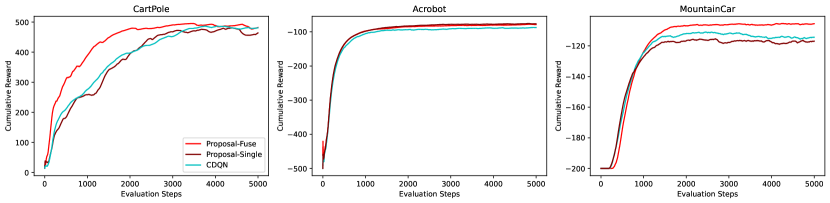
Figure 3: Comparison of our proposed methods using single and fused kernels. We report the mean of cumulative rewards across 10 independent runs.

References

- Bellemare et al. (2017) Bellemare, M. G., Dabney, W., and Munos, R. A distributional perspective on reinforcement learning. In International Conference on Machine Learning, pp. 449–458. PMLR, 2017.
- Bellemare et al. (2023) Bellemare, M. G., Dabney, W., and Rowland, M. Distributional Reinforcement Learning. MIT Press, 2023. http://www.distributional-rl.org.
- Biggs et al. (2023) Biggs, F., Schrab, A., and Gretton, A. MMD-FUSE: Learning and combining kernels for two-sample testing without data splitting. 2023. URL https://arxiv.org/abs/2306.08777.
- Bishop (1994) Bishop, C. M. Mixture density networks. Report NCRG/94/004, 1994.
- Chau et al. (2021) Chau, S. L., Ton, J.-F., Gonzalez, J., Teh, Y. W., and Sejdinovic, D. BayesIMP: Uncertainty Quantification for Causal Data Fusion. In Advances in Neural Information Processing Systems (NeurIPS), volume 34, pp. 3466–3477, 2021.
- Chen et al. (2010) Chen, Y., Welling, M., and Smola, A. Super-samples from kernel herding. In Proceedings of the 26th Conference on Uncertainty in Artificial Intelligence, pp. 109–116. AUAI Press, 2010.
- Dabney et al. (2018) Dabney, W., Rowland, M., Bellemare, M., and Munos, R. Distributional reinforcement learning with quantile regression. In Proceedings of the AAAI Conference on Artificial Intelligence, volume 32, 2018.
- Donsker & Varadhan (1975) Donsker, M. D. and Varadhan, S. R. S. Asymptotic evaluation of certain markov process expectations for large time. Communications on Pure and Applied Mathematics, 28(1):1–47, 1975.
- Dua & Graff (2017) Dua, D. and Graff, C. Uci machine learning repository, 2017. URL http://archive.ics.uci.edu/ml.
- Durkan et al. (2019) Durkan, C., Bekasov, A., Murray, I., and Papamakarios, G. Neural spline flows. In Advances in Neural Information Processing Systems, pp. 7509–7520, 2019.
- Fukumizu et al. (2004) Fukumizu, K., Bach, F. R., and Jordan, M. I. Dimensionality reduction for supervised learning with reproducing kernel hilbert spaces. In Journal of Machine Learning Research, volume 5, pp. 73–99, 2004.
- Fukumizu et al. (2008) Fukumizu, K., Gretton, A., Sun, X., and Schölkopf, B. Kernel measures of conditional dependence. In Advances in Neural Information Processing Systems, pp. 489–496, 2008.
- Fukumizu et al. (2013) Fukumizu, K., Song, L., and Gretton, A. Kernel Bayes’ rule: Bayesian inference with positive definite kernels. Journal of Machine Learning Research, 14(82):3753–3783, 2013.
- Girosi et al. (1995) Girosi, F., Jones, M., and Poggio, T. Regularization theory and neural networks architectures. Neural Computation, 7(2):219–269, 1995. doi: 10.1162/neco.1995.7.2.219.
- Gretton et al. (2005) Gretton, A., Herbrich, R., Smola, A., Schölkopf, B., and Hyvärinen, A. Kernel methods for measuring independence. In Journal of Machine Learning Research, volume 6, pp. 2075–2129, 2005.
- Gretton et al. (2012) Gretton, A., Borgwardt, K. M., Rasch, M. J., Schölkopf, B., and Smola, A. A kernel two-sample test. Journal of Machine Learning Research, 13(25):723–773, 2012.
- Grünewälder et al. (2012) Grünewälder, S., Lever, G., Baldassarre, L., Patterson, S., Gretton, A., and Pontil, M. Conditional mean embeddings as regressors. In Proceedings of the 29th International Conference on Machine Learning, pp. 1823–1830. Omnipress, 2012.
- Han et al. (2022) Han, X., Zheng, H., and Zhou, M. CARD: Classification and regression diffusion models. In Advances in Neural Information Processing Systems, 2022.
- Hensman et al. (2013) Hensman, J., Fusi, N., and Lawrence, N. D. Gaussian processes for big data. In Proceedings of the Conference on Uncertainty in Artificial Intelligence, pp. 282–290, 2013.
- Hsu & Ramos (2019) Hsu, K. and Ramos, F. Bayesian learning of conditional kernel mean embeddings for automatic likelihood-free inference. In Proceedings of the Twenty-Second International Conference on Artificial Intelligence and Statistics, volume 89 of Proceedings of Machine Learning Research, pp. 2631–2640. PMLR, 2019.
- Kanagawa & Fukumizu (2014) Kanagawa, M. and Fukumizu, K. Recovering Distributions from Gaussian RKHS Embeddings. In Kaski, S. and Corander, J. (eds.), Proceedings of the Seventeenth International Conference on Artificial Intelligence and Statistics, volume 33 of Proceedings of Machine Learning Research, pp. 457–465, Reykjavik, Iceland, 2014. PMLR.
- Killingberg & Langseth (2023) Killingberg, L. and Langseth, H. The multiquadric kernel for moment-matching distributional reinforcement learning. Transactions on Machine Learning Research, 2023. ISSN 2835-8856.
- Kim & Scott (2012) Kim, J. and Scott, C. D. Robust kernel density estimation. Journal of Machine Learning Research, 13(82):2529–2565, 2012.
- Kingma & Ba (2015) Kingma, D. P. and Ba, J. Adam: A method for stochastic optimization. In International Conference on Learning Representations, 2015.
- Loshchilov & Hutter (2019) Loshchilov, I. and Hutter, F. Decoupled weight decay regularization. In International Conference on Learning Representations, 2019.
- Lueckmann et al. (2021) Lueckmann, J.-M., Boelts, J., Greenberg, D., Goncalves, P., and Macke, J. Benchmarking simulation-based inference. In Proceedings of The 24th International Conference on Artificial Intelligence and Statistics, volume 130 of Proceedings of Machine Learning Research, pp. 343–351. PMLR, 2021.
- Makansi et al. (2019) Makansi, O., Ilg, E., Çiçek, Ö., and Brox, T. Overcoming limitations of mixture density networks: A sampling and fitting framework for multimodal future prediction. In IEEE International Conference on Computer Vision and Pattern Recognition, 2019.
- Miyato et al. (2018) Miyato, T., Kataoka, T., Koyama, M., and Yoshida, Y. Spectral normalization for generative adversarial networks. In International Conference on Learning Representations, 2018.
- Mnih et al. (2015) Mnih, V., Kavukcuoglu, K., Silver, D., Rusu, A. A., Veness, J., Bellemare, M. G., Graves, A., Riedmiller, M., Fidjeland, A. K., Ostrovski, G., et al. Human-level control through deep reinforcement learning. Nature, 518(7540):529–533, 2015.
- Muandet et al. (2017) Muandet, K., Fukumizu, K., Sriperumbudur, B., Schölkopf, B., and Gretton, A. Kernel mean embedding of distributions: A review and beyond. Foundations and Trends® in Machine Learning, 10(1-2):1–141, 2017.
- Muandet et al. (2021) Muandet, K., Kanagawa, M., Saengkyongam, S., and Marukatat, S. Counterfactual mean embeddings. Journal of Machine Learning Research, 22(162):1–71, 2021.
- Nguyen-Tang et al. (2021) Nguyen-Tang, T., Gupta, S., and Venkatesh, S. Distributional reinforcement learning via moment matching. Proceedings of the AAAI Conference on Artificial Intelligence, 35(10):9144–9152, 2021.
- Obando-Ceron & Castro (2021) Obando-Ceron, J. S. and Castro, P. S. Revisiting rainbow: Promoting more insightful and inclusive deep reinforcement learning research. In Proceedings of the 38th International Conference on Machine Learning, Proceedings of Machine Learning Research. PMLR, 2021.
- Papamakarios & Murray (2016) Papamakarios, G. and Murray, I. Fast -free inference of simulation models with bayesian conditional density estimation. In Advances in Neural Information Processing Systems, volume 29, pp. 1028–1036, 2016.
- Papamakarios et al. (2021) Papamakarios, G., Nalisnick, E., Rezende, D. J., Mohamed, S., and Lakshminarayanan, B. Normalizing flows for modeling and inference. Journal of Machine Learning Research, 22(57):1–64, 2021.
- Park et al. (2021) Park, J., Shalit, U., Schölkopf, B., and Muandet, K. Conditional distributional treatment effect with kernel conditional mean embeddings and u-statistic regression. In Proceedings of 38th International Conference on Machine Learning, volume 139 of Proceedings of Machine Learning Research, pp. 8401–8412. PMLR, 2021.
- Puterman (2014) Puterman, M. L. Markov decision processes: Discrete stochastic dynamic programming. John Wiley & Sons, 2014.
- Rezende & Mohamed (2015) Rezende, D. J. and Mohamed, S. Variational inference with normalizing flows. In Proceedings of The 32nd International Conference on Machine Learning, volume 37, pp. 1530–1538. PMLR, 2015.
- Saitoh (1997) Saitoh, S. Integral transforms, reproducing kernels and their applications. Pitman research notes in mathematics series ; 369. Chapman and Hall/CRC, 1997.
- Schaul et al. (2016) Schaul, T., Quan, J., Antonoglou, I., and Silver, D. Prioritized experience replay. In International Conference on Learning Representations, 2016.
- Singh et al. (2019) Singh, R., Sahani, M., and Gretton, A. Kernel instrumental variable regression. In Advances in Neural Information Processing Systems, volume 32, pp. 4595–4607, 2019.
- Song et al. (2009) Song, L., Huang, J., Smola, A., and Fukumizu, K. Hilbert space embeddings of conditional distributions with applications to dynamical systems. In International Conference on Machine Learning, pp. 961–968, 2009.
- Song et al. (2013) Song, L., Fukumizu, K., and Gretton, A. Kernel embeddings of conditional distributions: A unified kernel framework for nonparametric inference in graphical models. IEEE Signal Processing Magazine, 30(4):98–111, 2013.
- Sriperumbudur et al. (2010) Sriperumbudur, B. K., Gretton, A., Fukumizu, K., Schölkopf, B., and Lanckriet, G. R. Hilbert space embeddings and metrics on probability measures. Journal of Machine Learning Research, 11:1517–1561, 2010.
- Stimper et al. (2023) Stimper, V., Liu, D., Campbell, A., Berenz, V., Ryll, L., Schölkopf, B., and Hernández-Lobato, J. M. normflows: A pytorch package for normalizing flows. Journal of Open Source Software, 8(86):5361, 2023.
- Sugiyama et al. (2010) Sugiyama, M., Takeuchi, I., Suzuki, T., Kanamori, T., Hachiya, H., and Okanohara, D. Conditional density estimation via least-squares density ratio estimation. In Proceedings of the Thirteenth International Conference on Artificial Intelligence and Statistics, volume 9 of Proceedings of Machine Learning Research, pp. 781–788. PMLR, 2010.
- Towers et al. (2023) Towers, M., Terry, J. K., Kwiatkowski, A., Balis, J. U., Cola, G. d., Deleu, T., Goulão, M., Kallinteris, A., KG, A., Krimmel, M., Perez-Vicente, R., Pierré, A., Schulhoff, S., Tai, J. J., Shen, A. T. J., and Younis, O. G. Gymnasium, 2023. URL https://zenodo.org/record/8127025.
- van Hasselt et al. (2016) van Hasselt, H., Guez, A., and Silver, D. Deep reinforcement learning with double q-learning. In Proceedings of the Thirtieth AAAI Conference on Artificial Intelligence, pp. 2094–2100. AAAI Press, 2016.
- Virtanen et al. (2020) Virtanen, P., Gommers, R., Oliphant, T. E., Haberland, M., Reddy, T., Cournapeau, D., Burovski, E., Peterson, P., Weckesser, W., Bright, J., van der Walt, S. J., Brett, M., Wilson, J., Millman, K. J., Mayorov, N., Nelson, A. R. J., Jones, E., Kern, R., Larson, E., Carey, C. J., Polat, İ., Feng, Y., Moore, E. W., VanderPlas, J., Laxalde, D., Perktold, J., Cimrman, R., Henriksen, I., Quintero, E. A., Harris, C. R., Archibald, A. M., Ribeiro, A. H., Pedregosa, F., van Mulbregt, P., and SciPy 1.0 Contributors. SciPy 1.0: Fundamental Algorithms for Scientific Computing in Python. Nature Methods, 17:261–272, 2020.
- Watkins & Dayan (1992) Watkins, C. J. and Dayan, P. Q-learning. Machine learning, 8(3-4):279–292, 1992.
- Xu et al. (2021) Xu, L., Chen, Y., Srinivasan, S., de Freitas, N., Doucet, A., and Gretton, A. Learning deep features in instrumental variable regression. In International Conference on Learning Representations, 2021.
- Xu et al. (2022) Xu, L., Chen, Y., Doucet, A., and Gretton, A. Importance weighted kernel Bayes’ rule. In Proceedings of the 39th International Conference on Machine Learning, volume 162 of Proceedings of Machine Learning Research, pp. 24524–24538. PMLR, 2022.