Abstract

The current thesis aims to explore the reinforcement learning field and build on existing methods to produce improved ones to tackle the problem of learning in high-dimensional and complex environments. It addresses such goals by decomposing learning tasks in a hierarchical fashion known as Hierarchical Reinforcement Learning.

We start in the first chapter by getting familiar with the Markov Decision Process framework and presenting some of its recent techniques that the following chapters use. We then proceed to build our Hierarchical Policy learning as an answer to the limitations of a single primitive policy. The hierarchy is composed of a manager agent at the top and employee agents at the lower level.

In the last chapter, which is the core of this thesis, we attempt to learn lower-level elements of the hierarchy independently of the manager level in what is known as the ”Eigenoption”. Based on the graph structure of the environment, Eigenoptions allow us to build agents that are aware of the geometric and dynamic properties of the environment. Their decision-making has a special property: it is invariant to symmetric transformations of the environment, allowing as a consequence to greatly reduce the complexity of the learning task.

Contents

1. Acknowledgments
2. 1 Reinforcement Learning Framework
3. 1 Markov Decision Process
   1. 1.1 Value Functions
   2. 1.2 MDP Properties
4. 2 Dynamic Programming
   1. 2.1 Bellman Equations
   2. 2.2 Iterative Learning
      1. 2.2.1 Value Functions Iteration
      2. 2.2.2 Policy Iteration
      3. 2.2.3 Temporal Difference
5. 3 Gradient Methods
   1. 3.1 Regularization functions
   2. 3.2 Convex optimization perspective
   3. 3.3 Trust Region Policy Optimization
      1. 3.3.1 TRPO recipe
      2. 3.3.2 TRPO Algorithm:
   4. 3.4 Experiment
6. 2 Hierarchical Reinforcement Learning
   1. 4 Hierarchical Reinforcement Learning Methods
      1. 4.1 Hierarchical RL models
      2. 4.2 Related work
   2. 5 Hierarchical Reinforcement Learning via Information Maximization
      1. 5.1 Regularized Information Maximization
      2. 5.2 Objective function
      3. 5.3 On-Policy HRL:
      4. 5.4 Hierarchical Kullback-Leibler bound
      5. 5.5 Algorithm and Experiments
7. 3 Spectral Framework for options discovery
   1. 6 Proto-Value Functions and Spectral Clustering
      1. 6.1 Laplacian Operator and Spectral Clustering
         1. 6.1.1 Graph cut and Laplacians
         2. 6.1.2 Graph Laplacians
         3. 6.1.3 Cuts optimization
   2. 7 Eigenoption Discovery
      1. 7.1 Optimization on Matrix Manifold
      2. 7.2 Neural Network for Eigenvectors learning
         1. 7.2.1 Spectral Net
         2. 7.2.2 Spectral Inference Networks
      3. 7.3 Proposed Spectral Network
   3. 8 Evaluating the Spectral Network
      1. 8.1 Eigenvectors of the 4-rooms environment
      2. 8.2 Clustering
8. Conclusion

Chapter 1 Reinforcement Learning Framework

Abstract

We introduce the Markov Decision Process paradigm, some approximate Dynamic Programming methods, their counterparts in continuous space states, and lay their fundamentals, which will be used in the next chapters.

Abstract

We introduce HRL as a way to tackle the learning scaling problem and sparsity. We review some recent approaches used to learn decision hierarchies, and conclude with an on-policy hierarchical reinforcement learning method based on the work of Osa and Sugiyama [11] for an off-policy .

Abstract

After working on temporal action abstractions, we tackle the problem of state space abstraction to learn options on basis functions induced from the graph of the environment. We use spectral basis functions to learn representations that reflect the geometric dynamics of the environment.

Introduction

Reinforcement Learning (Sutton and Barto [1]) is a mathematical framework for active learning from experience. The concept is based on developing agents capable of learning in an environment through trial-and-error. The environment consists of a set of states $S$ and actions $A$. The agent interacts with the environment by moving from one state to another and receives feedback about its decisions through rewards. The goal of the agent is to learn a decision-making process, also called a policy, that maximizes the expected accumulated reward.

Based on this definition, we can already distinguish between two different types of Reinforcement Learning, depending on the prior knowledge about the environment: model-based and model-free. In the first type of RL, the dynamics of the environment are known prior to the learning process, and the agent incorporates the knowledge of the transition process between states (the laws of physics in a robotics task, for example). In contrast, in the second type, the agent has no prior knowledge about the environment dynamics and needs to acquire it while learning the best policy. In this work, we address model-free RL.

In this chapter, we introduce the Markov Decision Process paradigm (MDP) and summarize its fundamentals.

1 Markov Decision Process

In standard RL models, the agent is represented as a time-homogeneous Markov Decision Process (MDP). An MDP is a tuple $\Omega=(\mathcal{S},\mathcal{A},\mathcal{R},\mathcal{P})$ where $\mathcal{S}$, $\mathcal{A}$ are respectively the state and action spaces, $\mathcal{P}$ is the transition kernel where $P(s_{t+1}|s_{t},a_{t})$ represents the probability of transition from state $s_{t}$ to a new state $s_{t+1}$ when taking the action $a_{t}$. Each decision of taking action $a_{t}$ at state $s_{t}$ can yield a certain reward $R(s_{t},a_{t})$ which we assume is bounded and deterministic given $s_{t}$ and $a_{t}$. In the case of an infinite horizon, future rewards can be discounted with a factor $\gamma$ and the MDP becomes $\Omega=(\mathcal{S},\mathcal{A},\mathcal{R},\mathcal{P},\gamma)$, which will be our MDP of interest in this work.

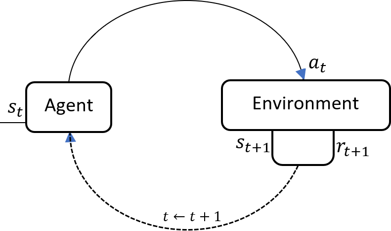
Figure 1: MDP structure

The goal in Reinforcement Learning (RL) is to permit the agent to learn autonomously, through trial and error, a policy $\pi:\mathcal{S}\times\mathcal{A}\rightarrow[0,1]$ that allows to maximize the expected accumulated rewards $\eta(\pi)$ defined as:

$$\eta(\pi)=\mathbb{E}^{\pi}\left[\sum_{t=0}^{\infty}\gamma^{t}r(s_{t})\right]\text{,}$$ (1)

where $\mathbb{E}^{\pi}$ means:

• $s_{0}\sim\rho_{0}$, $\rho_{0}$ is the initial distribution over the state space

• The action is then distributed following $a_{t}\sim\pi(.|s_{t})$.

• The next states follow $s_{t+1}\sim P(.|s_{t},a_{t})$

The time homogeneity implies that at any time $t$ we have:

$$P(s_{t+1}=s^{\prime}|s_{t}=s,a_{t}=a)=P(s^{\prime}|s,a)$$

1.1 Value Functions

Value functions measure the expected return conditioned on starting state and/or actions: the state-action value function $Q_{\pi}:\mathcal{S}\times\mathcal{A}\rightarrow\mathbb{R}$, and state value function $V_{\pi}:\mathcal{S}\rightarrow\mathbb{R}$ both defined with respect to policy $\pi$:

$$Q_{\pi}(s,a) =\mathbb{E}_{s_{t},a_{t},\dots}\left[\sum_{t=0}^{\infty}\gamma^{t}r(s_{t})|s_{0}=s,a_{0}=a\right]\text{,}$$ (2)

$$V_{\pi}(s) =\mathbb{E}_{a_{t},s_{t},\dots}\left[\sum_{t=0}^{\infty}\gamma^{t}r(s_{t})|s_{0}=s\right]\text{,}$$ (3)

and define the advantage function:

$$A_{\pi}(s,a)=Q_{\pi}(s,a)-V_{\pi}(s)$$

The value $Q_{\pi}(s,a)$ is the expected accumulated reward when taking the action $a$ at state $s$. When we sample this action $a$ following the policy $\pi(.|s)$, then we expect to accumulate $V_{\pi}(s)$. The advantage $A_{\pi}(s,a)$, on the other hand, translates the gain of taking the action $a$ in state $s$ instead of following the policy $\pi$. Consequently, the policy is optimal if the advantage is non-positive at each state for any adversary action $a$.

1.2 MDP Properties

Each policy induces a distribution over the state space which is proportional to the ”unnormalized” state density $\rho_{\pi}$ defined as

$$\rho_{\pi}(s) =\mathbb{E}^{\pi}\left[\sum_{t=0}^{\infty}\gamma^{t}\mathbbm{1}_{s_{t}=s}\right]$$

$$=\mathbb{E}_{s_{0}\sim\rho_{0},a_{t}\sim\pi(.|s_{t})}{\sum_{i=0}^{\infty}\gamma^{t}P(s_{t+1}=s|s_{t},a_{t})}\text{.}$$ (4)

Using $\rho_{\pi}$, the expected return $\eta(\pi)$ can be formulated as:

$$\eta(\pi)=\int_{\mathcal{S}}\int_{\mathcal{A}}\rho_{\pi}(s)\pi(a|s)r(s,a)dsda$$ (5)

We can also simplify $V_{\pi}$ using the initial density $\rho_{0}$:

$$\eta(\pi)=\mathbb{E}_{s_{0}\sim\rho_{0}}{V_{\pi}(s_{0})}\text{,}$$ (6)

This simple property can be used to prove the following important lemma, which links the discounted density with and the expected return of two policies (see [2] for proof):

Lemma 1.1.

Let $\pi$ and $\tilde{\pi}$ be two policies over the states space $\mathcal{S}$, we have the following

$$\eta(\pi)=\eta(\tilde{\pi})+\mathbb{E}^{\tilde{\pi}}\left[\sum_{t}\gamma^{t}A_{\pi}(s_{t},a_{t})\right],$$ (7)

and using the density $\rho_{\pi}$ :

$$\eta(\pi)=\eta(\tilde{\pi})+{\int_{\mathcal{S}}}{\int_{\mathcal{A}}}\rho_{\tilde{\pi}}(s)\tilde{\pi}(a|s)A_{\pi}(s_{t},a_{t})$$ (8)

This lemma, as discussed in subsection 1.1, implies that a policy update $\pi\leftarrow\tilde{\pi}$ with non-negative expected advantage over $\pi$ at every state will increases $\eta(\pi)$.

Remarks

In the remaining study, we restrict our interest to the following MDP s

• $r:\mathcal{S}\times\mathcal{A}\rightarrow\mathbb{R}$ is deterministic given the state and action

• The transition mechanism from $s_{t}$ to $s_{t+1}$ given $a_{t}$ is deterministic

While deterministic rewards apply to a large set of environments, using a prior distribution on the reward has recently been proven to improve many of the reinforcement learning models, even when the reward is deterministic [3]. It has also been proven that in distributional RL, some of the properties of MDP change, such as the contraction property of the Bellman operator, which we’ll define in the following section.

2 Dynamic Programming

Dynamic Programming (DP) [4] is mathematical optimization paradigm developed by Richard Bellman in the 1950s. It mainly specializes in optimization problems where the sub-problems can be nested recursively inside the general one. Using Bellman equations with specific assumptions on the objective function, we are guaranteed to have a link between the general solution and the sub-problems solutions. In our case, we can notice that for two consecutive states $s_{t},s_{t+1}$, if a policy $\pi$ maximizes $V_{\pi}(s_{t})$ then it necessarily maximizes $V_{\pi}(s_{t+1})$.

2.1 Bellman Equations

The Bellman equations applied to the value functions can be written as follows:

$$V_{\pi}(s) =\mathbb{E}_{a\sim\pi(.|s)}\left[r(s,a)+\gamma\mathbb{E}_{s^{\prime}\sim P(.|s,a)}\left[V_{\pi}(s^{\prime})\right]\right]$$ (9)

$$Q_{\pi}(s,a) =r(s,a)+\gamma\mathbb{E}_{s^{\prime}\sim P(.|s,a)}\left[V_{\pi}(s^{\prime})\right].$$ (10)

We define the Bellman operators $\mathcal{T}_{\pi}:\mathbb{R}^{\mathcal{S}}\rightarrow\mathbb{R}^{\mathcal{S}}$ as:

$$\mathcal{T}_{\pi}(f)(s)=\mathbb{E}_{a\sim\pi(.|s)}\left[r(s,a)+\gamma\mathbb{E}_{s^{\prime}\sim P(.|s,a)}\left[f(s^{\prime})\right]\right],$$ (11)

and the optimal Bellman operator $\mathcal{T^{*}}:\mathbb{R}^{\mathcal{S}\times\mathcal{A}}\rightarrow\mathbb{R}^{\mathcal{S}\times\mathcal{A}}$ as:

$$\mathcal{T^{*}}(f)(s)=\max_{a}\left[r(s,a)+\gamma\mathbb{E}_{s^{\prime}\sim P(.|s,a)}\left[f(s^{\prime})\right]\right]$$ (12)

Both $\mathcal{T}_{\pi}$ and $\mathcal{T^{*}}$ are contractions with Lipschitz constant $\gamma$. Hence, both admit unique fixed points and we can conclude that:

• Every policy $\pi$ defines unique value functions $V_{\pi}$ and $Q_{\pi}$

• There is unique optimal value function $V^{*}$, the fixed point of $\mathcal{T^{*}}$, which verifies:

  $$V^{*}(s)=\max_{a}\mathbb{E}_{\pi(.|s)}\left[r(s,a)+\gamma\mathbb{E}_{s^{\prime}\sim P(.|s,a)}\left[V^{*}(s^{\prime})\right]\right]$$

The optimal action value function $Q^{*}$ can be induced:

$$Q^{*}(s,a) =r(s,a)+\gamma V^{*}(s)$$

$$=r(s,a)+\gamma\max_{a}\mathbb{E}_{s^{\prime}\sim P(.|s,a)}\left[\max_{a^{\prime}}Q^{*}(s^{\prime},a^{\prime})\right]$$

These properties, however, do not imply the uniqueness of the optimal/greedy policy $\pi^{*}$ associated with the optimal functions:

$$\pi^{*}(a|s)=\mathbbm{1}_{\operatorname*{arg\,max}_{a}Q_{\pi^{*}}(s,a)}$$

Based on the advantage function $A^{*}$, if two actions $a_{1}$ and $a_{2}$ at a certain state $s$ verify $A^{*}(s,a_{1})=0$ and $A^{*}(s,a_{2})=0$, then we are indifferent between the two as they both have the same future accumulated discounted rewards.

2.2 Iterative Learning

Based on the Bellman equations and the properties of the operators, we introduce in this section different methods used to learn the optimal value functions and/or the optimal policies. The iterative learning is used for finite MDP, but they share many fundamentals with their counterparts in continuous state MDP. It is important to note that the presented methods belong to the approximate Dynamic Programming, where we attempt to approximate value functions and policies. The approximation quality depends on the richness of the family of functions on which we optimize (least-square, neural networks…).

As noted in subsection 2.1, since the Bellman operators are contraction mappings, we have the following result:

Theorem 1.1 (Contraction mapping theorem).

Let $\mathcal{X}$ be a complete metric space, and $F:\mathcal{X}\rightarrow\mathcal{X}$ be a contraction. Then $F$ has a unique fixed point, and under the action of iterates of $F$, all points converge with exponential speed to it.

Using Bellman operators, by starting from any random function $f_{0}:\mathcal{S}\rightarrow\mathbb{R}$ and defining $f_{n}=\mathcal{T}^{n}(f_{0})$, then $(f_{n})_{n}$ converges to the fixed point of $\mathcal{T}$. While this applies to both V and Q functions, it is generally preferable to learn the action value $Q$ (or the advantage $A$) function since they allow inducing the optimal action at each state. Learning only $V$, however, requires knowledge of either the reward or the temporal difference $V(s_{t+1})-V(s_{t})$, implying prior knowledge about the transition mechanism to predict the next state.

2.2.1 Value Functions Iteration

Using the contraction mapping property, we can iteratively approximate the value function $V$ in a discrete infinite time horizon MDP:

Algorithm 1 Value Iteration Algorithm

An initial value function $V:\mathcal{S}\rightarrow\mathbb{R}$

for $t\leftarrow 1\textrm{ to }T$ do

     $s_{0}\sim\rho_{0}$

     Sample a trajectory $\tau=(a_{0},s_{1},s_{2}...s_{n})$

     Estimate $V_{t+1}\leftarrow T^{*}(V_{t})$ based on $\tau$

end for

Return: The greedy policy associated with $V_{T}$

The same algorithm can be applied to the state-action function $Q_{t}$. The updates can be performed in an asynchronous fashion by updating the value function at each step of the trajectory. The trajectory sampling can be done in an on-policy manner by using the greedy policy $\pi_{t}$ at iteration $t$, or in an off-policy way. The on-policy method can imply a risk of staying in a local domain of the state space. The common practice is to add stochasticity with an $\epsilon-$greedy method by choosing random actions with probability $\epsilon$. The contraction mapping property guarantees convergence only if all states can be visited infinitely often. This is known as the exploitation-exploration dilemma in RL, since we want to exploit the learned knowledge while being able to explore new states once in a while.

2.2.2 Policy Iteration

In a similar way to Value Iteration (VI), Policy Iteration (PI) starts with an initial policy $\pi_{0}$ then alternates between learning $V_{\pi}$ and $\pi$.

Algorithm 2 Policy Iteration Algorithm

An initial value policy $\pi_{0}$

for $t\leftarrow 1\textrm{ to }T$ do

     Sample a trajectory $\tau=(s_{0},a_{0},s_{1},s_{2}...s_{n})$

     Evaluate ${V_{\pi}}_{t}$

     $\pi_{t+1}\leftarrow{\pi^{*}}_{t}$ with ${\pi^{*}}_{t}$ the greedy policy of ${V_{\pi}}_{t}$

     Estimate $V_{t+1}\leftarrow T^{*}(V_{t})$ based on $\tau$

end for

Return: The learned policy $\pi_{T+1}$

The same thing about exploration-exploitation applies to PI. The PI and VI methods assume that we can efficiently estimate $V_{\pi,t}$ and $\pi_{t}$, which are practically challenging, since the value functions are formulated as the expectations of the policy and initial distribution. Practically, we sample one or several trajectories and estimate the expectation over the trajectories and incrementally update the previous quantities.

2.2.3 Temporal Difference

When starting from a state $s_{t}$ and taking action $a_{t}$ to observe $s_{t+1}$, the one-step temporal difference error is defined as:

$$\Delta_{t}\vcentcolon=r(s_{t},a_{t})+\gamma{V_{\pi}}^{(n)}(s_{t+1})-{V_{\pi}}^{(n)}(s_{t}),$$ (13)

with ${V_{\pi}}^{(n)}$ being the value function estimation at iteration $n$ and $r(s_{t},a_{t})+\gamma{V_{\pi}}^{(n)}(s_{t+1})$ the TD target.

For $\lambda\in[0,1]$, the $\lambda$-temporal difference TD($\lambda$) is used to update the estimated function:

$${V_{\pi}}_{n+1}(s_{t})\leftarrow{V_{\pi}}_{n}+\alpha_{n}\sum_{s=0}\lambda^{s}\Delta_{s}.$$

The parameter $\lambda\in[0,1]$ is called the trace decay. A higher $\lambda$ reflects lasting reward traces, with $\lambda=1$ the value function update is performed at the end of the trajectory, while for $\lambda=0$ the update is performed after each decision step. The update rate $(\alpha_{i})$ is generally chosen to satisfy the Robbins-Monro condition:

$$\sum_{i}\alpha_{i} =\infty$$ (14)

$$\sum_{i}\alpha_{i}^{2} <\infty$$ (15)

Given enough samples, the Robbins-Monro condition guarantees that the approximations $({V_{\pi}}^{(n)})_{n}$ converge almost surely to the true $V_{\pi}$.

The temporal difference error plays an important role in continuous and large space state MDP, and it is largely used for $Q$ and $V$ function learning (SARSA[5], Q-learning[1]). Its main advantage is that it can be applied in high-dimensional state space MDP using differentiable approximations. In the following section, we will be exposing some of these methods.

3 Gradient Methods

In continuous and high-dimensional state space MDP, Temporal Difference is the core of several approximate DP models. The most basic methods use parameterized functions (Least Squares, Neural Networks) and attempt to update the parameters to minimize $TD(\lambda)$ using closed-form solutions or gradients depending on the parameterization. Neural Networks have gained popularity for their ease of use in gradient descent methods and their ability to scale RL techniques to high-dimensional state space.

In this section, we go beyond the simple applications of $TD(\lambda)$ to briefly present a particular class of gradient methods: policy gradient methods. We summarize the work of Neu et al.. In their work on unifying policy gradient methods, they reintroduce 3 popular policy gradient methods from a convex optimization point of view:

• Relative Entropy Search (REPS) (2010)

• Trust Region Policy Optimization (TRPO) (2015)

• Asynchronous Actor-Critic Agents (A3C) (2016)

They demonstrate that these methods aim to solve the same objective using different constraints.

3.1 Regularization functions

We define the Shannon entropy $E_{S}$ for a policy $\pi$ as

$$E_{S}(\pi)\vcentcolon=\sum_{s,a}\pi(x,a)\log\pi(x,a),$$ (16)

and the negative conditional entropy $E_{c}$ :

$$E_{C}(\pi)\vcentcolon=\sum_{s,a}\pi(s,a)\log\dfrac{\pi(s,a)}{\sum_{b}\pi(s,b)}.$$ (17)

To constrain the policy updates, we use the Bregman divergences $D_{S}$ and $D_{C}$ associated with the entropies $E_{S}$ and $E_{D}$, respectively, defined as:

$$D_{S}(\pi\|\tilde{\pi})\vcentcolon=\sum_{s,a}\pi(s,a)\log\dfrac{\pi(s,a)}{\tilde{\pi}(s,a)}$$ (18)

$$D_{C}(\pi\|\tilde{\pi})\vcentcolon=\sum_{s}\pi(s)\sum_{a}\pi(a|s)\log\dfrac{\pi(a|s)}{\tilde{\pi}(a|s)}$$ (19)

$E_{S}$ and $E_{C}$ are two strictly convex functions over the space of distributions on the $\mathcal{S}\times\mathcal{A}$. $D_{S}$ is in fact the Kullback-Leibler divergence while $D_{C}$ is known as the conditional KL divergence over the state space.

3.2 Convex optimization perspective

With regularization functions defined above, Neu et al. proved that at the $t$ gradient update of the policy, all the three methods attempts to solve the following objective :

$$\pi_{t+1}=\operatorname*{arg\,max}_{\pi}\Bigl{(}\eta(\pi)-\alpha.D(\pi\|\pi_{t})\Bigr{)},$$ (20)

where D being the divergence associated with the method.

REPS

uses mirror descent with Bregman divergence $D_{S}$ in 20.

$$\pi_{t+1}=\operatorname*{arg\,max}_{\pi}\Bigl{(}\eta(\pi)-\alpha.D_{S}(\pi\|\pi_{t})\Bigr{)}.$$

In each update $t$, the trajectories are sampled using the current policy $\pi_{t}$. Using Lagrangian strong duality and the strict convexity of the entropy $E_{S}$, REPS is equivalent to the mirror descent algorithm using the Bregman divergence $D_{S}$. Consequently, REPS converges to the optimal policy. However, as is the case for all other methods, the optimality is relative to the class of parameterized functions on which we optimize the objective in (20).

TRPO

solves 20 using the Bregman divergence $D_{C}$. TRPO formulates the problem as:

$$\begin{aligned} &\underset{x}{\text{maximize}}&&\eta(\pi)\\ &\text{subject to}&&D_{C}(\pi\|\pi_{t})\leq\delta,\end{aligned}$$ (21)

where $\delta$ is a hyper-parameter controlling the update step. TRPO determines the trust region update using conjugate gradient to bound the divergence.

A3C

accumulates gradients of the objective (20) with regularization $D_{C}$. The gradients are provided asynchronously from several agents. Instead of using mirror descent, it uses the dual averaging method by incorporating updates provided by the agents. However, in their unified framework, Neu et al. argue that A3C does not present any convergence guarantees. The interesting result is that the optimal update in the case of A3C has a closed form:

$$\pi_{t+1}\propto\exp{\frac{A_{\pi_{k}}}{\beta_{k}}},$$ (22)

where ($\beta_{k}$) an increasing sequence to insure convergence.

3.3 Trust Region Policy Optimization

TRPO optimizes the objective (21) by first replacing the discounted state density $\rho_{\tilde{\pi}}$ in Equation 8 with $\rho_{\pi}$. The obtained the quantity is:

$$L_{\pi}(\tilde{\pi})=\eta(\pi)+\sum_{s}\rho_{\pi}(s)\sum_{a}\tilde{\pi}(a|s)A_{\pi}(s,a).$$ (23)

$L_{\pi}(\tilde{\pi})$ is a first-order approximation of $\eta(\tilde{\pi})$. At this stage, we consider parameterized policies $(\pi_{\theta})_{\theta\in\mathbb{R}^{n}}$ and we use $\theta$ to design $\pi_{\theta}$. Schulman et al. proved the following inequality, analogous to the Conservative Policy Iteration (CPI):

Lemma 1.2.

$$\eta(\theta)\geq L_{\theta_{\mathrm{old}}}(\theta)-C{D^{\rm max}_{\rm KL}}(\theta_{\mathrm{old}},\theta).$$ (24)

Maximizing the right side of the inequality improves (remains constant in the worst case) the surrogate. TRPO proceeds by relaxing the bound based on $D_{KL}^{max}$ and the objective becomes:

$$\operatorname*{maximize}_{\theta}L_{\theta_{\mathrm{old}}}(\theta)$$ (25)

$$\text{\ \ subject to }{\overline{D}_{\rm KL}^{\rho_{\theta_{\mathrm{old}}}}}(\theta_{\mathrm{old}},\theta)\leq\delta.$$

${D^{\rm max}_{\rm KL}}$ is the maximum KL divergence between policies over the sampled states, while ${\overline{D}_{\rm KL}}$ is the mean KL divergence.

3.3.1 TRPO recipe

By simulating trajectories following the current policy, we estimate the objective and the bound:

• Expand $L_{\theta_{\mathrm{old}}}$ in Equation (25), we replace $\sum_{s}\rho_{\theta_{\mathrm{old}}}(s)\left[\dots\right]$ in the objective by the expectation $\frac{1}{1-\gamma}\mathbb{E}_{s\sim\rho_{\theta_{\mathrm{old}}}}\left[\dots\right]$

• Replace $A_{\theta_{\mathrm{old}}}$ by the $Q$-values $Q_{\theta_{\mathrm{old}}}$ in Equation (23),

• replace the sum over the actions by an importance sampling estimator based on ${\pi_{\theta}}_{old}$.

TRPO problem is hence equivalent to the following one:

$$\operatorname*{maximize}_{\theta}\mathbb{E}_{s\sim\rho_{\theta_{\mathrm{old}}},a\sim q}\left[\frac{\pi_{\theta}(a|s)}{{\pi_{\theta}}_{old}(a|s)}Q_{\theta_{\mathrm{old}}}(s,a)\right]$$ (26)

$$\text{\ \ subject to }\mathbb{E}_{s\sim\rho_{\theta_{\mathrm{old}}}}\left[D_{\rm KL}(\pi_{\theta_{\mathrm{old}}}(\cdot|s)\ \|\ \pi_{\theta}(\cdot|s))\right]\leq\delta.$$

3.3.2 TRPO Algorithm:

Algorithm 3 Trust Region Policy Optimization

A parameterized policy $\pi_{\theta}$ and $\theta$=$\theta_{0}$

for $i\leftarrow 1\textrm{ to }T$ do

     Run policy for N trajectories

     Estimate advantage function at all time steps

     Compute objective gradient $g_{\theta}$

     Compute A

     Use Conjugate Gradient to compute $\beta$ and $s$

     Compute the rescaled update line search

     Apply update to $\theta$

end for

We denote by $g_{\theta}$ the gradient of the objective with respect to $\theta$. We write the quadratic approximation of the constraint function :

$${\overline{D}_{\rm KL}}(\theta_{\mathrm{old}},\theta)\approx\frac{1}{2}(\theta-\theta_{\mathrm{old}})^{T}A(\theta-\theta_{\mathrm{old}}),$$

where

$$A_{ij}=\frac{\partial}{\partial\theta_{i}}\frac{\partial}{\partial\theta_{j}}{\overline{D}_{\rm KL}}(\theta_{\mathrm{old}},\theta).$$

Since $A$ is symmetric semi-definite, we use the conjugate gradient method to solve $s=Ag_{\theta}$. The solution $s$ is the search direction. We then obtain the maximal step scale $\beta=\sqrt{2\delta/s^{T}As}$ that verifies $\delta={\overline{D}_{\rm KL}}\approx\frac{1}{2}(\beta s)^{T}A(\beta s)=\frac{1}{2}\beta^{2}s^{T}As$. The last step is the line search, which allows us to shrink the step exponentially until the objective improves.

3.4 Experiment

We test the TRPO algorithm in the ”4-room” environment. The motivation for such a choice of environment is the ability to compare results between continuous space, where we use the raw RGB screen as input, and the exact solutions in the tabular case. The agent (white square) goal is to reach the red square to receive a $+1$ reward, in the minimal number of steps. The horizon is virtually infinite, but practically sufficient to explore all states before episodes end. We can also expand the state space by expanding the grid’s size. For a size: $n=36$ and randomly located white and red squares, the total number of states is of the order of $10^{6}$. We can also control the sparsity by varying the number of red squares.

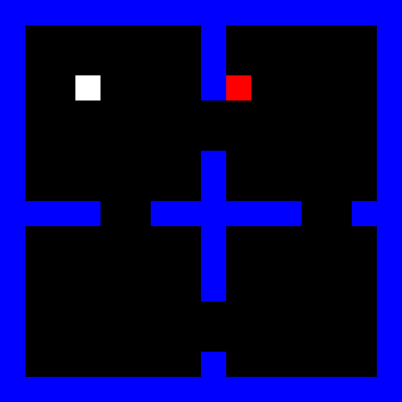
(a) $n=16$

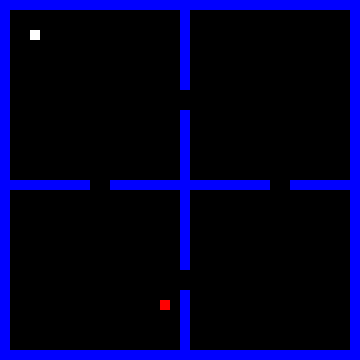
(b) $n=36$

Figure 2: 4-room environment for different sizes

Our implementation of the TRPO agent is a PyTorch adaptation of the official TensorFlow implementation from OpenAI baselines [10]. We’ve tested the implementation on some of the Atari Games, and the scores were similar to the ones reported in [8]. However, for the 4-room environment with a large size in the stochastic framework (the target red square is randomly located), the TRPO fails to improve the policy. When reaching the goal, it quickly forgets the experience. This is mainly due to the sparsity of the rewards.

We plot below the mean time to the goal for each room size. We start from the uniform policy. The plots are moving averages of 5 runs. We’ve also run the algorithm stagnates at the maximum episode length.

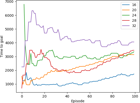
Figure 3: TRPO in 4 Rooms

Conclusion

After presenting the fundamentals of Reinforcement Learning in a multi-state space, we summarized Neu et al.’s unifying framework for entropy-regularized policy gradient methods. We tested the TRPO algorithm on a few environments and demonstrated some of its limitations in a sparse environment.

In the following chapter, we attempt to tackle these limitations in the framework of the Hierarchical Reinforcement Learning (HRL) by extending the TRPO to incorporate task hierarchies.

Chapter 2 Hierarchical Reinforcement Learning

Introduction

As is the case with human learning, biological organisms can master tasks from extremely small samples. The fact that a child can acquire a visual object concept from a single unlabeled example is evidence for preexisting cortical mechanisms that facilitate such efficient learning [12]. While reinforcement learning is rooted in Neuroscience and Psychology [13], Hierarchical Reinforcement Learning was developed in the machine learning field based on the abstraction of either the states or the actions.

State abstraction [14, 15] is based on learning a state representation concentrating on features relevant to the decision process and excluding the irrelevant ones; hence, behaviorally similar states should induce the same representation. On the other hand, action abstraction is based on using temporally extended policies [16] to scale the learning task. Once a temporally abstract action is initiated, the execution of its associated policy continues until a set of specified termination states is reached. Thus, the selection of a temporally abstract action ultimately results in the execution of a sequence of actions.

In this chapter, we focus on temporal action abstraction for a continuous state MDP. We start with an overview of related work on which we proceed to build our method.

4 Hierarchical Reinforcement Learning Methods

While Hierarchical Learning is based on a features hierarchy, hierarchical RL is based on a hierarchy of tasks. At the top of the structure, a manager designates an employee with an assigned goal. The employee attempts to accomplish the goal to get the reward before a termination condition is met (it gets fired). Employees can be their own managers for other sub-employees, which is known as ”Feudal Reinforcement Learning” [17] with the ”manager” (Lord) policy at the top and ”sub-managers” at lower levels of the hierarchy receiving sub-goals from their ”super-managers”.

Some of the earlier work on HRL used the terms ”primitive actions” and ”macro-actions”. In [18], Hauskrecht et al. introduced the macro-actions as local policies that act in certain regions of the state space. The ”primitive action” policy then clusters the state space and assigns each macro-action to a specific state space domain.

In this thesis, we will use the terms gate or gating policy for the primitive actions, and ”option” policies for the macro-actions.

4.1 Hierarchical RL models

An option is a tuple $(I_{o},\pi_{o},T_{o})$, where $I_{o}\subset\mathcal{S}$ is the initiation set, $\pi_{o}$ is the option’s policy, and $T_{o}\subset\mathcal{S}$ is the termination set (stopping time). The gating policy, in a similar way to the primitive policies from the first chapter, is a mapping $\pi_{g}:\mathcal{S}\times\mathcal{O}\rightarrow[0,1]$ from the state space to the distributions over the option set $\mathcal{O}=\{o_{i}|i\in I\}$, the set of options. Following the same notations of the first chapter, we denote the gating policy by $\pi_{g}$ and $\pi(.|s,o)$ the policy of the option $o$.

We define the hierarchical policy as:

$$\pi(a|s)=\sum_{o\in\mathcal{O}}\pi_{g}(o|s)\pi(a|s,o).$$ (27)

Using the discounted state distribution $\rho_{\pi}$ as in equation ( 5), the objective becomes:

$$\eta(\pi)=\int_{\mathcal{S}}\int_{\mathcal{A}}\rho_{\pi}(s)\sum_{o\in\mathcal{O}}\pi_{g}(o|s)\pi(a|s,o)r(s,a)dsda$$ (28)

Several methods used this structure as in the [19] and [11], where, besides the raw state, the gate provides the option with a latent variable $o$ called ”goal” or ”sub-goal”. In the case of a sub-goal, the options maximize the expected accumulated intrinsic reward returned from an internal critic.

In a more general framework, the hierarchical policy picks an option at times $S_{t}=\sum_{l=1}^{t}T_{o_{l}}$, where $o_{l}$ is the option drawn at round $l$. Between $S_{t}$ and $S_{t+1}$, the actions are chosen following option $o_{t}$. We can write the objective $\eta(\pi)$ as:

$$\eta(\pi)=\mathbb{E}^{\pi}\left[\sum_{t=1}^{\infty}\gamma^{S_{t-1}}\sum_{u=0}^{T_{t}}\gamma^{u}r(s_{t},a_{t})\right].$$

Ultimately, the HRL model should also learn the stopping time for each option.

4.2 Related work

In their hierarchical adaptation of the DQN [20], Kulkarni et al. used a gate (meta-controller) and options (controllers) to attain handcrafted goals. While the gate tries to maximize the accumulated reward from the environment (extrinsic reward), the options maximize an intrinsic reward from the internal critic by achieving the assigned goals. The abstract action terminates when the episode ends or the goal is reached. Their method succeeded in solving the ”MontezumaRevenge Atari” game, in which the non-hierarchical methods fail to score. However, the hDQN goals were handcrafted and hence needed input that can be expensive.

For an on-policy variant, Daniel et al. [19] introduced several Hierarchical REPS variants (see section 3 in chapter 1). The option policies in Hierarchical Relative Entropy Search (HREPS) were allowed to share experiences (inter-option learning), the chosen option was a hidden latent representation that the model tries to infer using Expectation-Maximization. The inference is based on a sampled trajectory, in which each policy $o_{i}$ attempts to ”claim” its responsibility $p(o_{i}|s,a)$ for action $a$ at state $s$. To avoid concurrence between policies, HREPS constrains the entropy of options’ responsibilities.

Among the recent research on HRL, Harutyunyan et al. in [21] addressed the learning of the option’s stopping time $T_{o}$. In the call-and-return HRL model, as in h-DQN, an option is run until completion. In their paper, they argued for the efficiency of shorter option policies and derived a method to learn the termination condition in an off-policy. In our work, however, this aspect is not treated, and we restrict our study to fixed option duration.

As pointed out in [18], the gating policy performs a clustering of the state space domain. While in HREPS [19], option policies could achieve the same performance on some domains of the state space. This indicates that the choice of the optimal gating policy $\pi_{g}$, if achievable, isn’t unique. Since we treat $o$ as a latent variable, in analogy with HREPS, we need to impose additional constraints to obtain a preferable solution. For the choice of the constraint, we opt for Regularization via Information Maximization (RIMs).

5 Hierarchical Reinforcement Learning via Information Maximization

To learn the hierarchical policy, we impose a regularization on the latent variable $o$. The hierarchical policy $\pi$ then attempts to optimize the objective:

$$\mathcal{L}(\pi)=\eta(\pi)+\mathcal{R}(\pi),$$ (29)

where $\eta(\pi)$ was defined in Equation 28.

We choose to impose a mutual information constraint on the gating policy. In the Regularised Information Maximization (RIM) framework, $\eta(\pi)$ is considered the regularization term of $\pi$.

5.1 Regularized Information Maximization

In Unsupervised Learning, Mutual Information measures have been shown to produce interpretable latent representations, especially in the clustering task ([22], [23], [24]). Following the previously discussed models, learning the gating policy in our model is similar to performing a clustering of the state space and assigning each option to a specific domain. It is hence justified to leverage Mutual Information (MI) performance in the HRL task.

The gating policy, a discrete distribution over $\mathcal{O}$, is the representation $O$ and $X=(s_{i},a_{i})_{i}$ the observed variable. We define the empirical mutual information:

$$\hat{I}(O,X)=\hat{H}(O)-\hat{H}(O|X),$$ (30)

where $\hat{H}(O)$ is the empirical estimate of entropy $H(O)=\int p(o)\text{log}(p(o))=\mathbb{E}\left[\text{log}(p(O))\right]$ using the empirical distribution:

$$\hat{p}(o)={\frac{1}{n}}\sum_{i=1}^{n}p(o|s_{i},a_{i}),$$

and $\hat{H}(O|X)$ is the empirical estimate of $H(O|X)$

$$\hat{H}(O|X)={\frac{1}{n}}\sum_{i=1}^{n}p(o_{i}|s_{i},a_{i})\text{log}(p(o_{i}|s_{i},a_{i})),$$

with: $p(o|s,a)=\frac{\pi(a|s,o)\pi_{g}(o|s)}{p(a|s)}$, and $p(a|s)=\sum_{o\in\mathcal{O}}\pi_{g}(o|s)\pi(a|s,o)$

Adding the regularizing quantity $\hat{\mathcal{R}}(\pi)$ to the objective $\eta_{\pi}$ incentivizes the gating policy to uniformly sample option policies by increasing $H(O)$, while at the same time, clearly distinguishing between each option’s domain by decreasing $H(O,X)$.

5.2 Objective function

We fix the number of options policies $|O|=k$ and we consider a deterministic termination set $\mathcal{T_{o}}=\tau$. We consider the hierarchical policy as in (27). The hierarchical policy’s objective :

$$\eta(\pi)=\int_{\mathcal{S}}\int_{\mathcal{A}}\rho_{\pi}(s)\sum_{o\in\mathcal{O}}\pi_{g}(o|s)\pi_{o}(a|s,o)r(s,a)dsda-\lambda I(O,S),$$ (31)

for a given parameter $\lambda$.

Since we will be using parametric approximation, we note $\pi_{\theta}$ the policy with parameter $\theta$. In a similar way to TRPO notations, we use $\theta$ indices to refer to quantities defined using $\pi_{\theta}$.

5.3 On-Policy HRL:

The TRPO model incorporates an estimation of the advantage function $A_{\pi}$, which can be used to model the gating policy using the softmax probabilities. Then the probability of choosing the option $i$:

$$\pi(o|s,a)=\frac{exp[A(s,\pi_{i}(s)|o_{i})]}{\sum_{j}exp[A(s,\pi_{j}(s)|o_{j})]}$$ (32)

This would allow to decouple the learning of the latent variable o and the gating policy, since the distribution on options only depend on their estimation advantages. From the HREPS and hierarchical Deep Q Learning (h-DQN) methods introduced, we can either

• In a similar way to REPS, allow inter-option learning

• Make each policies value estimation hidden from the gating policy. This implies that the gating policy should estimate its own value function as well. This similar to the h-DQN method.

In this work, we present a different method where each option learns only from its own experience while the gating policy is oblivious to the advantages estimation (we won’t use softmax Q).

5.4 Hierarchical Kullback-Leibler bound

To extend the TRPO to hierarchical policies, we use the following lemma (see proof Chapter 2 proofs in Appendix).

Lemma 2.1.

Let $n\geq 1$ be the number of option policies, and $\pi_{g}$ the gating policy (distribution over the options set). If $\pi$ and $\tilde{\pi}$ are two hierarchical policies such that $\tilde{\pi}$ is absolutely continuous with respect to $\pi$, then at any state $s$, we have:

$$\text{D}_{\text{KL}}(\pi(.|s)|\tilde{\pi}(.|s)\leq\text{D}_{\text{KL}}(\pi_{g}(.|s),\tilde{\pi}_{g}(.|s))+\sum_{o\in\mathcal{O}}\pi_{g}(o|s)\text{D}_{\text{KL}}(\pi(.|s,o)|\tilde{\pi}(.|s,o))).$$ (33)

The right side’s second term is, in fact, the Bregman divergence for the conditional entropy but with an expectation over the options set instead of the state space as seen in Chapter 1.

In a similar work [25], Michalewski used a hierarchy of parameters. Instead of drawing an option, the gating policy chooses the subspace for the option’s parameters. The options then belong to the family of multivariate Gaussians. This choice of structure turns the inequality in 33 into an equality, as the divergence between two hierarchies over the same option vanishes.

Based on 33, to bound the KL divergence, it’s sufficient to bound both the gate and the options. We can also use adaptive bounds for the options by bounding $\pi_{g}(o|s)\text{D}_{\text{KL}}(\pi(.|s,o)|\tilde{\pi}(.|s,o)))$ instead of $\text{D}_{\text{KL}}(\pi(.|s,o)|\tilde{\pi}(.|s,o)))$.

5.5 Algorithm and Experiments

Algorithm 4 Trust Region Hierarchical Policy Optimization

A parameterized gate policy $\pi_{\theta}$ and option policies $(\pi_{o_{i},\theta})$

for $i\leftarrow 1\textrm{ to }T$ do

     Run policy for N trajectories

     Estimate the advantage

     Calculate the Mutual Information Measure

     Use Trust Region method to get the update step wrt to the gate

     Update Step

     for  each option i do

         Get the Objective after last update

         Use the trust region method for the option i

         Apply update

     end for

end for

The trust region method mentioned in the algorithm is the same one used in standard TRPO, by using a quadratic approximation of the KL divergence, then exploiting the Fisher vector product and using conjugate gradient. The objective needs to be calculated after each update and also incorporate gradient graphs for each policy when using neural networks. In practical terms, it requires large GPU memory when naively implemented. A trickier way would imply stopping the gradient from policies uninvolved in the optimization step.

We compare the performance of the TRHPO method with the TRPO in the 4 rooms environment. We use the same neural network architectures for the gating and option policies and the TRPO policy with the same KL bounds.

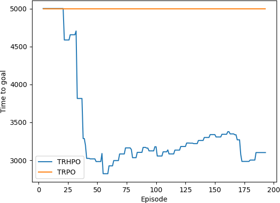
Figure 4: TRHPO vs TRPO in 4 Rooms

While the TRPO performance is far from optimal, it outperforms the TRPO method in MDPs with sparse rewards, a known advantage of hierarchical methods.

We also plot the exploited options during the learning process:

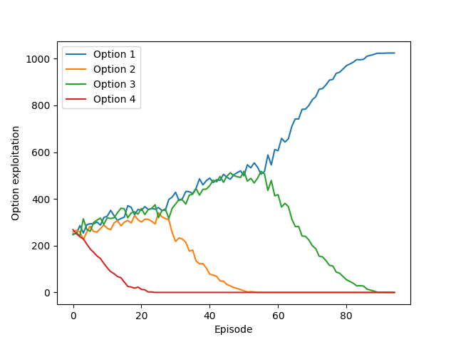
Figure 5: TRHPO exploited options

Conclusion

Despite outperforming simple TRPO, the TRHPO gradually excludes option policies to only exploit one option policy around the 90th episode. At the end of the first 100 episodes, the algorithm reaches a local optimum. In our tests, convergence to local optima limits the TRHPO performance in a range of environments, especially where the reward isn’t sparse.

After building the hierarchical policy learning method, we aim next to incorporate options that can be learned independently of the top-level policies. We aim to achieve such a goal by generalizing the Proto-Value Function (PVF) concept to solve the MDP on specific basis functions.

Chapter 3 Spectral Framework for options discovery

Introduction

Another way of learning the value functions or policies is to approximate them on a certain basis functions. This approach has several applications in Machine Learning[26] (Fourier Wavelets, Laplacian) and Quantum Physics (Hamiltonian)[27] and yields good results when the right basis is used. The most recent one perhaps is the $100\%$ accuracy on MNIST using complex neural networks built on the frequency domain features[28]

In the context of RL, the concept of Proto-Value Function (PVF) introduced by Mahadevan[29] uses the eigenvectors of the graph Laplacian as basis to learn the optimal policy for a discrete state space MDP. The idea is to exploit the geometry of the environment since spatially close states can be ”dynamically” far or even separate. In the 4-room environment in the examples, $state_{1}$ is visually closer to $state_{2}$ than $state_{3}$, but dynamically further than it.

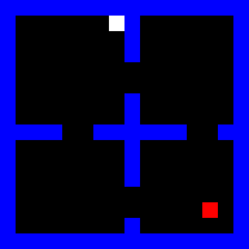
(a) $state_{1}$

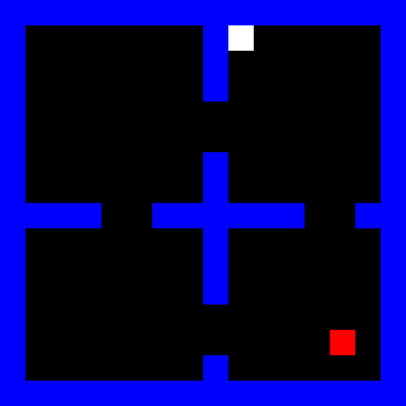
(b) $state_{2}$

(c) $state_{3}$

Figure 6: Euclidian distance and geodesic distance

In this chapter, we will introduce the Proto-Value Function (PVF) paradigm, present the Laplacian operator and its use in Spectral Clustering before integrating it into our study of RL. Since we are interested in applications for high-dimensional state space, we will present and evaluate our model for scaling the introduced techniques.

6 Proto-Value Functions and Spectral Clustering

The PVF [29] introduced a spectral framework for approximate dynamic programming. It mainly addressed a finite state space MDP setting in model-free RL. The overall framework can be summarized as follows: the agent constructs the adjacency matrix of the state space graph where the similarity $W_{i,j}=1$ if the agent could move from state $s_{i}$ to state $s_{j}$. The diffusion model is defined using the normalized symmetric graph Laplacian $L_{sym}$. Then the basis functions are simply the smoothest eigenvectors of the Laplacian (associated with the lowest eigenvalues). To learn the optimal policy, PVF uses ”Representation Policy Iteration,” a policy iteration that takes the projection on the smoothest eigenvectors as states.

To illustrate the concept, we use a 4-room environment with a size of $16\times 16$ (177 accessible states). We consider the fixed starting point with an absorbing goal state. We have 176 states, for which we plot in ( 7) the optimal value function $V*$ and its approximation on the first 5 and the full Laplacian basis, learned using Least Square Policy Iteration (LSPI). Contrary to what we might conclude visually from (7(b)), using the smoothest 5 eigenvectors doesn’t solve the problem. In fact, the approximated policy has absorbing states different from the target state. Solving this issue requires using more eigenvectors which in turn creates new modes in the approximated function, hence the need for a sufficiently large basis to nullify the discontinuity. Several works address this problem by using a smoother basis as in Sugiyama et al. where the geodesic Gaussian kernels are used to build similarities based on the shortest path distance.

In an entirely different perspective, with the concept of ”Eigenoptions”, Machado et al. learns options that maximize intrinsic rewards induced by the eigenvectors. This allows creating options that reflect the geometric properties translated by each eigenvector separately. Afterwards, a policy over the Eigenoptions is used to associate each eigenoption with a certain domain of the state space, similar to hierarchical RL.

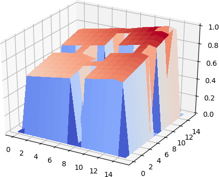
(a) Optimal $V^{*}$

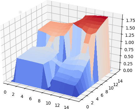
(b) Using 5 eigenvectors

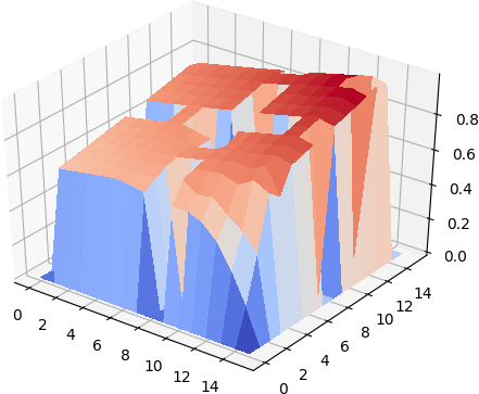
(c) using 177 eigenvectors

Figure 7: Optimal $V$ and approximations

In the subsequent section, we delve into fundamental properties of the graph Laplacian that will be utilized subsequently to introduce eigenoptions.

6.1 Laplacian Operator and Spectral Clustering

Spectral clustering[32] addresses the problem of partitioning an undirected weighted graph $G=(V,E)$ under specific constraints, where $V$ represents the set of vertices and $E$ the set of edges.

Let $V=\{{v_{1},...,v_{n}}\}$, and $W$ the $n\times n$ adjacency matrix where $W_{i,j}$ is the non-negative weight of the edge linking $v_{i}$ and $v_{j}$, and $W_{i,j}=0$ means that the vertices $v_{i}$ and $v_{j}$ are not linked. The undirected nature of the $G$ means that $W$ is symmetric. We define the degree of the vertex $v_{i}$ as $d_{i}=\sum_{j}W_{i,j}$ and the degree matrix $D=\operatorname{diag}{(d_{1},....,d_{n})}$.

Let $A\subset V$, we define the indicator vector $1_{A}=(f_{1},.....f_{n})$ as: $f_{i}=1_{v_{i}\in A}$. Similarly, we can measure the similarity between two subsets $A$ and $B$ by the sum of the ”similarity” between their vertices:

$$W(A,B):=\sum_{i\in A,j\in B}w_{i,j}=1_{A}^{T}W1_{B}\text{ ,}$$

and to measure the size of the set $A$, we can either use:

• The cardinality measure :

  $$\text{vol}_{\text{c}}(A)\vcentcolon=|A|=1_{A}^{T}1_{A}$$

  .

• Total of its elements degrees:

  $$\text{vol}_{\text{d}}(A)\vcentcolon=\sum_{i\in A}d_{i}=1_{A}^{T}D1_{A}$$

  .

6.1.1 Graph cut and Laplacians

To partition the graph $G$ into two separate sets $A$ and $\overline{A}$, Spectral Clustering searches for the least ”similar” sets $A$ and $B$. We can use two types of similarity measures:

$$\text{Ratiocut}(A,\overline{A})\vcentcolon=\frac{W(A,\overline{A})}{|A|}$$ (34)

$$\text{Ncut}(A,\overline{A})\vcentcolon=\frac{W(A,\overline{A})}{\text{vol}_{\text{d}}(A)}$$ (35)

We can prove the following properties:

$$\text{Ratiocut}(A,\overline{A}) =\frac{{\mathbbm{1}_{A}}^{T}(D-W)\mathbbm{1}_{A}}{{\mathbbm{1}_{A}}^{T}\mathbbm{1}_{A}}$$ (36)

$$\text{Ncut}(A,\overline{A}) =\frac{{\mathbbm{1}_{A}}^{T}(D-W){\mathbbm{1}_{A}}}{{\mathbbm{1}_{A}}^{T}D\mathbbm{1}_{A}}$$ (37)

Since we are interested in finding the set $A$, distinct from $V$, the partitioning problem is then formulated as finding the vector of $\mathbb{R}^{n}$ with $\{0,1\}$ elements that minimizes the Rayleigh quotient in Equation Equation 36 or Equation 37.

6.1.2 Graph Laplacians

Unnormalized/Combinatorial Laplacian:

The combinatorial Laplacian, appearing in the Ratiocut, is defined as $L\vcentcolon=D-W$, which has the following properties:

• for $f$ in $\mathbb{R}^{n}$

  $$f^{T}Lf=\sum w_{i,j}(f_{i}-f_{j})^{2}$$

• L is symmetric semi definite

• The smallest eigenvector is $1$ for the eigen value $\lambda_{0}=0$

• In particular, self-edges in a graph do not change the corresponding graph Laplacian

Normalized Laplacians:

Spectral Clustering literature uses two types of normalized Laplacians:

• Random Walk $L_{rw}=I-D^{-1}W$

• Symmetric, appearing in the Ncut, $L_{sym}=I-D^{-{\frac{1}{2}}}WD^{-{\frac{1}{2}}}$

The matrix $T=D^{-1}W$ can be viewed as a transition matrix. Although $L_{rw}$ is not symmetric, all its eigenvalues are real, non-negative, and upper-bounded by $1$. The normalized Laplacians exhibit the following properties:

• For $f\in\mathbb{R}^{n}$:

  $$f^{T}L_{sym}f={\frac{1}{2}}\sum_{i,j}(\frac{f_{i}}{\sqrt{d_{i}}}-\frac{f_{j}}{\sqrt{d_{j}}})^{2}$$ (38)

• $u$ is an eigenvector of $L_{r}w$ with eigen value $\lambda$ iif $W=D^{{\frac{1}{2}}}u$ is an eigenvector of $L_{s}ym$ for the same eigen value.

6.1.3 Cuts optimization

Solving Equation 36 and Equation 37 on the set $\{0,1\}^{n}$ is an NP-hard problem. To address this challenge, we relax the constraint such that the unknown function $f$ is dense with a specific norm. Minimizing the Ratiocut involves identifying the minimizer $f$ of the Rayleigh quotient for the matrix $L$, subject to the conditions $f^{T}f=\sqrt{n}I$ and $f^{T}\mathbbm{1}_{V}=0$.

For the Ncut, the objective is to determine $g=D^{{\frac{1}{2}}}\mathbbm{1}_{A}$, which is the minimizer of the Rayleigh quotient for $L_{sym}$. This is achieved under the constraints $g^{T}g=\sqrt{n}I$ and $g^{T}D^{{\frac{1}{2}}}\mathbbm{1}_{V}=0$. The minimizer of the Rayleigh quotient, subject to these specified constraints, corresponds to the smoothest eigenvector of the matrices (excluding the first eigenvector).

Consequently, vertices within the same subset are anticipated to exhibit similar projections onto the solutions of the relaxed problem. As we ascend the Laplacian spectrum, the projections onto the eigenvectors are inclined to capture more distinct (higher frequency) variations. Therefore, possessing knowledge of the complete spectrum is expected to yield representations that effectively differentiate all vertices.

7 Eigenoption Discovery

Eigenoptions[31] are based on a simple property of the eigenvectors. Plotting the first 3 eigenvectors below, the agent starts at position $(3,3)$ and has to reach $(33,33)$. Let $\phi_{i}$ be the $i-th$ eigenvector, and we define the intrinsic reward $r_{i}$ for taking action $a$ to transition $s\rightarrow^{\prime}$

$$r_{i}(s,a)=\phi_{i}(s^{\prime})-\phi_{i}(s)$$

The $i$-th Eigenoption is the policy that maximizes the expected accumulated intrinsic reward $r_{i}$. In Figure 8, the first Eigenoption would lead the agent to the corner of the first room an and exit the third room. For the third Eigenoption, the agent would have to exit the second and fourth room to reach the absorbing state in the corners of the first and third room. So if the task is to exit the first room, we should follow the second eigenoption.

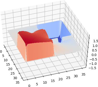
(a) $1^{st}$ eigenvector

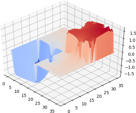
(b) $2^{nd}$ eigenvector

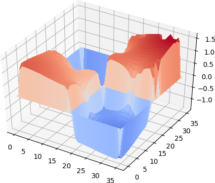
(c) $3^{rd}$ eigenvector

Figure 8: Eigenvectors of $L_{sym}$

Extending the concept of Eigenoptions to large and continuous state space MDP requires to be able to learn eigen vectors of large, and virtually infinite, graph Laplacian. In this section we go through two recent methods and in the last section we present our own.

7.1 Optimization on Matrix Manifold

For problems involving orthogonality or low-rank constraints, these characteristics are expressed naturally using the Grassmann manifold. There has been growing interest in studying the Grassmann manifold and exploiting its structure, especially in computer vision. However, the manifold structure was usually used to model either the input or the parameters of parametric functions. It is only recently that we’ve started to see works where neural networks are used to output representations on the manifold. More specifically, given a batch sample $(X_{i})_{i\leq n}$ in $\mathbb{R}^{d}$, we want to learn a mapping $F:\mathbb{R}^{d}\rightarrow\mathbb{R}^{k}$ that solves:

$$\begin{aligned} &\underset{F}{\text{minimize}}&&\mathcal{L}((X_{i})_{i},F)=\sum_{i,j\leq n}K(X_{i},X_{j})F(X_{i})^{T}F(X_{j})\\ &\text{subject to}&&{\frac{1}{n}}\sum_{i}F(X_{i})^{T}F(X_{i})=I_{k},\end{aligned}$$ (39)

with K a similarity kernel on $\mathbb{R}^{d}\times\mathbb{R}^{d}$.

In other words, the $n\times k$ matrix $Y$ with rows $Y_{i}={\frac{1}{\sqrt{n}}}F(X_{i})$ should be on the Stiefel manifold defined as:

$$V_{n,k}\vcentcolon=\{A\in\mathbb{R}^{n}\times\mathbb{R}^{k}|A^{T}A=I_{k}\}$$

However, the problem doesn’t have a unique solution. Given an optimal mapping F and taking a matrix $Q\in\mathcal{O}_{k}$ to define ${F^{\prime}}(X)=F(X)^{T}Q$, then ${F^{\prime}}$ is also optimal.

To correctly define the problem, the optimization set should identify elements of $V_{n,k}$ whose columns span the same subspace: the Grassmann manifold $G_{n,k}$.

When $n$ is large, evaluating whether $F$’s outputs are on the Grassmann manifold can be only approximated. Informally, if the input X has distribution P, then $F$ is simply transforming X into a latent representation such that:

$$\begin{aligned} &\underset{F}{\text{minimize}}&&\mathbb{E}^{P}[K(X,X^{\prime})F(X)^{T}F(X^{\prime})]\\ &\text{subject to}&&\mathbb{E}^{P}[F(X)^{T}F(X)]=I_{k},\end{aligned}$$ (40)

To evaluate if the output of batch of size $n$ is on the manifold, we use the distance:

$$d_{g}(A)=\underset{B\in G_{n,p}}{inf}{||A-B||_{2}^{2}}$$

Lemma 3.1.

For a matrix $A\in\mathbb{R}^{n}\times\mathbb{R}^{k}$:

$$d_{g}(A)=\sum_{i=1}^{k}(\sigma_{i}-1)^{2}$$ (41)

where $S=\operatorname{diag}(\sigma_{1},...\sigma_{k})$ such that $A=USV^{T}$ is the SVD decomposition of A.

Consequently, the projection of $A$ on Grassmann manifold is $B=UV^{T}$.

7.2 Neural Network for Eigenvectors learning

7.2.1 Spectral Net

In [33], Shaham et al. used neural networks to learn an approximation of Laplacian eigenvectors for large-scale applications. Their ’SpectralNet’ $f_{\theta}:\mathbb{R}^{n}\rightarrow\mathbb{R}_{k}$ tries to minimize the ”spectral loss” defined as:

$$L_{SpectralNet}(\theta,(x_{i})_{i})={\frac{1}{m^{2}}}\sum_{i,j=1}^{m}W_{i,j}\left\lVert f_{\theta}(x_{i})-f_{\theta}(x_{j})\right\rVert^{2},$$

under the constraint:

$${\frac{1}{m}}\sum_{i,j=1}f_{\theta}(x_{i})^{T}f_{\theta}(x_{j})=I_{k}.$$

The minimization is done with batches, and $m$ is the size of the batch. To impose the orthogonality constraint, a ”Cholesky” decomposition layer is added on top of the neural network.

Cholesky Layer:

Let $Y$ be the neural network’s output for a sample $X$ of size $m$. If we take the Cholesky decomposition $L$ of $S:={\frac{1}{m}}Y^{T}Y=LL^{T}$, where $L$ is a lower triangular matrix, then $Y^{*}=\sqrt{m}YL^{-1}$ is on the Grassmann manifold.

The paper’s main contribution, however, is establishing a theoretical result for the minimum number of units required to be able to learn the eigenvectors.

Lemma 3.2.

$$VCdim(F^{spectralclustering}_{n})\geq\frac{n}{10}.$$ (42)

This implies that to learn representation separating $n$ points, the number of weights in the neural net should be in the same order as the number of points $n$.

They have also demonstrated the convergence to real eigenvectors for some cases. On the other hand, the methods used for learning are based on simple back-propagation. At each iteration, the Cholesky layer weights are frozen to minimize the Spectral loss. Since the minimizer of such loss is the zero matrix, the output approaches zero while the Cholesky layer weight, the inverse of $L$ for $Y$ approaching $0$, can explode if the learning rate isn’t carefully controlled. Furthermore, the SpectralNet methods don’t address the overlapping of eigenvectors; hence, the representation learned is, in fact, a noisy combination of the smoothest eigenvector.

7.2.2 Spectral Inference Networks

Inspired by applications for the Hamiltonian in quantum mechanics, Pfau et al. addresses the general problem of maximizing the Rayleigh quotient for an ”infinite” matrix whose elements are defined by a certain similarity kernel.

$$\begin{aligned} &\underset{x}{\text{maximize}}&&\text{Tr}((Y^{T}Y)^{-1}Y^{T}AY)\\ &\text{subject to}&&Y^{T}Y=I_{k},\end{aligned}$$ (43)

where $A\in\mathbb{R}^{n,n}$ and $Y\in\mathbb{R}^{n,k}$.

Given an input data $(x_{i})_{i\leq n}$ and $(y_{i})_{i\leq n}$, their output using Spectral Inference Network (SpIn), and $A$ as their similarity matrix, we define $\Pi$ and $\Sigma$ in $\mathbb{R}^{k,k}$ as:

$$\Pi \vcentcolon={\frac{1}{n}}\sum_{i,j}a_{i,j}x_{i}{x_{j}}^{T}$$ (44)

$$\Sigma \vcentcolon={\frac{1}{n}}\sum_{i,i}x_{i}{x_{i}}^{T}$$ (45)

Using these notations, $\Sigma$ and $\Pi$ depend on the network parameter $\theta$, and the gradient of the objective can be written as:

$$\text{Tr}(\Sigma\nabla_{\theta}\Pi)-\text{Tr}(\Sigma^{-1}\Pi\Sigma^{-1}\nabla_{\theta}\Sigma)$$

To solve the objective, Pfau et al. proceeds by accumulating an empirical estimate of $\Sigma$ and $\nabla_{\theta}\Sigma$, which requires calculating $k^{2}$ gradients and storing $k^{2}$ times the number of network parameters. Based on the theoretical result of SpectralNet, approximating eigenvectors requires a large neural network. Therefore, calculating and storing $\nabla_{\theta}\Sigma$ is expensive.

On the other hand, SpIn addresses the question of overlapping eigenvectors and modifies the gradient in a way to make the update sequentially independent: the first eigenvectors’ gradient is independent of the gradient coming from eigenvectors of higher eigenvalues. In our implementation of the SpIn, modifying the gradient reduces the update step and hence renders the objective increments extremely slow. Furthermore, we believe that the sparsity constraints used in their neural network and the separation of weights of eigenvectors have an important impact on the performance demonstrated in their paper, which was considered a technical detail in their work.

7.3 Proposed Spectral Network

We build on SpectralNet and SpIn to derive a new method that produces separated eigenvectors, with fewer gradient backpropagations and memory requirements. Using the same notation in the previous subsection, we aim to minimize the ”Sequential” Rayleigh quotient. Let

$$R_{j}(A,Y)=\text{Tr}((Y_{j}^{T}Y_{j})^{-1}Y_{j}^{T}A_{:j,:j}Y_{j})$$

Where $Y_{j}$ is the matrix of the first $j$ vectors of $Y$ and $A_{:j,:j}$ is the first $j\times j$ block of matrix $A$.

Then our objective is:

$$\begin{aligned} &\underset{Y}{\text{minimizer}}&&\sum_{j}R_{j}(A,Y)\\ &\text{subject to}&&Y^{T}Y=I_{k},\end{aligned}$$ (46)

If the eigenvalues of $A$ are distinct, then the columns of the global optimum are guaranteed to be orthogonal.

From this point, the key idea is to take update directions for which the gradient $\nabla_{\theta}\Sigma$ is small and update the network parameters to minimize the Grassmann distance. This is similar in a way to the sub-gradient method. However, the set on which we incrementally project (Grassmann Manifold) is not convex in our case.

Furthermore, we use large samples to estimate the sequential Rayleigh quotient. Alternatively, we can use the learned covariance matrix as in the SpIn.

At iteration $t$, where the parameter of the network is $\theta_{t}$:

$$\begin{aligned} &\underset{\theta}{\text{minimize}}&&\sum_{j}R_{j}(A,Y_{\theta})\\ &\text{subject to}&&||Y_{\theta}^{T}Y_{\theta}-Y_{\theta_{t}}^{T}Y_{\theta_{t}}||_{2}^{2}=\delta.\end{aligned}$$ (47)

We note that $||Y_{\theta}^{T}Y_{\theta}-Y_{\theta_{t}}^{T}Y_{\theta_{t}}||_{2}^{2}$ is approximately quadratic in $\theta$ for $\theta$ sufficiently close to $\theta_{t}$. For a small $\delta$, the update step ensures staying approximately on the same Stiefel manifold as the covariance doesn’t change. After each step minimizing the objective, we take an orthogonal update towards the Grassmann manifold under the constraint of keeping the gained improvement. The learned covariance matrix is used to update the weight of the output Cholesky layer. The update is done gradually using a learning step instead of the brutal update as in SpectralNet. Ultimately, the Cholesky layer allows the network to output the centered eigenvectors based on the learned covariance matrix $\Sigma$.

Algorithm 5 Spectral Network

A parameterized network $F_{\theta}$, Learning rate $\alpha$ for $\Sigma$, Learning rate $\beta<1$ for gradient updates

for $i\leftarrow 1\textrm{ to }T$ do

     Sample $(x_{i})_{i}$ and get the output $(y_{i})_{i}$

      Calculate $\hat{\Sigma}$ and update the Cholesky layer weights with rate $\alpha$

      Get gradient of the Sequential Rayleigh quotient

      Use quadratic approximation of the constraint, calculate fisher information matrix

      Use Conjugate Gradient to find a search direction $g$

      Get the Grassmann distance gradient $p$ and project it on the normal on $g$

      Use Armijo line search using $g$

      Use a simple line search using $p$ while keeping approximately the gained improvement from previous step

     If Rayleigh Quotient doesn’t improve after 10 iterations, reduce update rate

end for

8 Evaluating the Spectral Network

We use our network to learn eigenvectors of the combinatorial Laplacian for the 4 rooms environment of size 36. Since the eigenvector associated with the first eigenvalue is the vector $1$, we can fix the first component of the output.

8.1 Eigenvectors of the 4-rooms environment

Two states are similar if the agent transitions from one to another. We consider the grid with size $36$ with random locations for the agent and the target point, which sums up to $1202312$ possible states. We use the combinatorial Laplacian in our experiment, since all positions have nearly the same degrees, except positions near the walls. Furthermore, using normalized Laplacians requires estimating the degree of vertices, which is prohibitively difficult in batch learning. To avoid sampling the same state multiple times, we use a graph builder that hashes the states and identifies states using the hash dictionary.

We visualize the finite set of states for the deterministic 4-room environment. The eigenvectors, however, have been learned for the stochastic 4-room environment, which has a space of over $10^{6}$ states. We display in the figures below the 3rd and the 5th learned eigenvectors for the deterministic environment and a second environment which is a 180 degrees rotation of the initial one.

The obtained functions display similar invariance characteristics with spectral eigenvectors. More importantly, learning eigenoptions using these ”eigenfunctions” will ensure that the learned options will lead to the same relative states. In our work, we attempted to use the TRPO model used in the first 2 chapters to learn eigenoptions, but without success. We believe it is due to the necessary large size of the network.

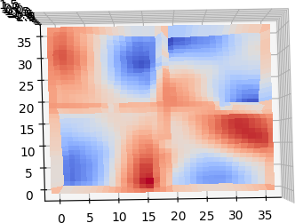
(a) Initial Environment

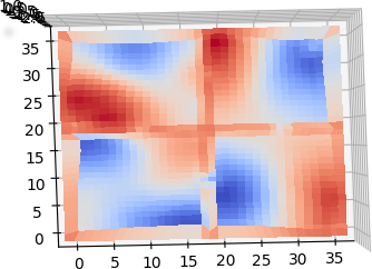
(b) Rotated Environment

Figure 9: 3rd Eigenvector

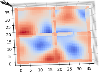
(a) Initial Environment

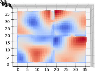
(b) Rotated Environment

Figure 10: 5th Eigenvector

8.2 Clustering

We also compare our method’s performance with the baseline in SpectralNet, which uses the spectral network without learning Siamese similarities or using the variational embedding of the dataset.

We define similarities between data points using nearest neighbors for $n=5$. To reduce the similarity variance between samples, we store the learned distances and keep the closest $1024$ neighbors from each point. This allows us to stabilize the similarities between data points once enough points are browsed. Using this method, it is unclear what number of eigenvectors to use, since there is no guarantee of having a fully connected graph or avoiding creating unnecessary cliques.

MNIST

For MNIST, we report have the following performance:

Number of eigenvectors	Accuracy	SpectralNet Score
10	69.27%	62.3%
11	71.08%	-
15	74.17%	-
20	67.85%	-

Reuters

For the Reuters dataset, we learn the first 4 eigenvectors. We train on $6.10^{5}$ data points and evaluate on a testing set of size $10^{4}$. We report a test accuracy of $76.18\%$ after 72 iterations, which drops to around $69\%$ afterwards. The training accuracy stabilizes around $67.24\%$. Since the training set is large, the reported training accuracy is evaluated between distant iterations. This is to be compared with the $64.5\%$ accuracy achieved by SpectralNet. Hence, we believe that using embedding or Siamese networks, as was done by Shaham et al., would outperform SpectralNet.

Conclusion

After building the HRL model, we attempted to learn options directly without going through the full HRL method. We used the PVF concept and built on recent work to approximate eigenvectors using neural networks for large datasets. We demonstrated that the learned functions present similar invariance characteristics as the Spectral eigenvectors and showed that our method outperforms the recent SpectralNet in the clustering task when used without Siamese distances nor the variational embedding.

On the other hand, we encountered difficulties when learning eigenoptions using the TRPO method. Therefore, we envision continuing to improve and build on the current achievements and to extend it to the standard use of eigenfunctions: Successor Features estimation.

Conclusion

Starting with the goal of building improved Reinforcement Learning methods, we showed that clustering the state space is an efficient strategy to master complex and large state spaces. First, using action abstraction by building the Hierarchical TRPO method. In the second part, we build on the Eigenoption method, which can be seen as a state abstraction, to learn the embedding of the state space incorporating the knowledge about environment dynamics.

We perform extensive tests for our method for learning the eigenvectors for clustering and for Eigenoptions estimation. Our next step was supposed to combine the Hierarchical model with Eigenoptions. As we have demonstrated, learning eigenfunctions requires large neural networks. Similarly, when learning an eigenoption, the option policy should be as rich as the spectral network to have a good approximation of the policy. This has hindered our testing of the HTRPO and limited our reported results for the RL task.

To tackle this problem, the model can be improved by incorporating more sophisticated parameterization as the sparse weight block used in [34]. In the immediate term, we will pursue more extensive tests of the developed model with more theoretical examination of the optimization heuristic.

Glossary

Acronyms

A3C

Asynchronous Actor-Critic Agents

CPI

Conservative Policy Iteration

DP

Dynamic Programming

h-DQN

hierarchical Deep Q Learning

HREPS

Hierarchical Relative Entropy Search

HRL

Hierarchical Reinforcement Learning

LSPI

Least Square Policy Iteration

MDP

Markov Decision Process

MI

Mutual Information

PI

Policy Iteration

PVF

Proto-Value Function

REPS

Relative Entropy Search

RIM

Regularised Information Maximization

RIMs

Regularization via Information Maximization

RL

Reinforcement Learning

SpIn

Spectral Inference Network

TRPO

Trust Region Policy Optimization

VI

Value Iteration

TRPO Implementation Parameters

Chapter 2 proofs

Lemma 3.3.

Let $n\geq 1$ be the number of option policies, and $\pi_{g}$ the gating policy (distribution over the options set). If $\pi$ and $\tilde{\pi}$ are two hierarchical policies such that $\tilde{\pi}$ is absolutely continuous w.r.t $\pi$, then at any state $s$, we have

$$\text{D}_{\text{KL}}\left[\tilde{\pi}(.|s)||\pi(.|s)\right]\leq\text{D}_{\text{KL}}\left[\tilde{\pi}_{g}(.|s)||\pi_{g}(.|s)\right]+\sum_{k=1}^{n}\pi_{g}(o|s)\text{D}_{\text{KL}}\left[\tilde{\pi}(.|s,o))||\pi(.|s,o)\right]$$ (48)

Proof.

We fix a state $s$, and we consider the two distributions p and q:

$$\begin{split}p(a,o)\vcentcolon=\pi(a,o|s)=\pi_{g}(o|s)\pi(a|s,o),\\ q(a,o)\vcentcolon=\tilde{\pi}(a,o|s)=\tilde{\pi}_{g}(o|s)\tilde{\pi}(a|s,o)\end{split}$$ (49)

and we denote $p_{A}$ and $q_{A}$, $p_{O}$ and $q_{O}$, respectively, the marginal distributions.

Using the conditional KL-divergence, we have th following two identities

$$\text{D}_{\text{KL}}\left[q||p\right]=\text{D}_{\text{KL}}\left[q_{A}||p_{A}\right]+\sum_{a}q_{A}(a)\text{D}_{\text{KL}}\left[q(.|a)||p(.|a)\right]$$ (50)

$$\text{D}_{\text{KL}}\left[q||p\right]=\text{D}_{\text{KL}}\left[q_{O}||p_{O}\right]+\sum_{o}q_{O}(o)\text{D}_{\text{KL}}\left[q(.|o)||p(.|o)\right]$$ (51)

Substracting Equation 51 from Equation 50, we obtain:

$$\text{D}_{\text{KL}}\left[q_{A}||p_{A}\right]=\text{D}_{\text{KL}}\left[q_{O}||p_{O}\right]+\sum_{o}q_{O}(o)\text{D}_{\text{KL}}\left[q(.|o)||p(.|o)\right]-\sum_{a}q_{A}(a)\text{D}_{\text{KL}}\left[q(.|a)||p(.|a)\right]$$ (52)

Since $\text{D}_{\text{KL}}\left[q(.|a)||p(.|a)\right]\geq 0$for all $a\in\mathcal{A}$, we have:

$$\text{D}_{\text{KL}}\left[q_{A}||p_{A}\right]\leq\text{D}_{\text{KL}}\left[q_{O}||p_{O}\right]+\sum_{o}q_{O}(o)\text{D}_{\text{KL}}\left[q(.|o)||p(.|o)\right]$$ (53)

All is left is to notice that :

$$p {}_{A}=\pi(.|s),\text{ }q_{A}=\tilde{\pi}(.|s)$$

$$p {}_{o}=\pi_{g}(.|s),\text{ }q_{o}=\tilde{\pi}_{g}(.|s)$$

$$p (.|o)=\pi(.|s,o),\text{ }q(.|o)=\tilde{\pi}(.|s,o).$$

Hence :

$$\text{D}_{\text{KL}}\left[\tilde{\pi}(.|s)||\pi(.|s)\right]\leq\text{D}_{\text{KL}}\left[\tilde{\pi}_{g}(.|s)||\pi_{g}(.|s)\right]+\sum_{o}\tilde{\pi}_{g}(o|s)\text{D}_{\text{KL}}\left[\tilde{\pi}(.|s,o)||\pi(.|s,o)\right]$$ (54)

∎

References

- Sutton and Barto [2017] Richard S. Sutton and Andrew G. Barto. Reinforcement Learning: An Introduction, Second Edition. The MIT Press, 2017. [View].
- Kakade and Langford [2002] Sham Kakade and John Langford. Approximately optimal approximate reinforcement learning. In In Proceedings of 19th International Conference on Machine Learning, pages 267–274, 2002. [View].
- Bellemare et al. [2017] Marc G. Bellemare, Will Dabney, and Rémi Munos. A distributional perspective on reinforcement learning. CoRR, abs/1707.06887, 2017. [View].
- Bellman [1954] Richard Bellman. The theory of dynamic programming. Bulletin of the American Mathematical Society, 60, 1954. [View].
- Rummery and Niranjan [1994] G. A. Rummery and M. Niranjan. On-line q-learning using connectionist systems. ., 1994. [View].
- Neu et al. [2017] Gergely Neu, Anders Jonsson, and Vicenç Gómez. A unified view of entropy-regularized markov decision processes. CoRR, abs/1705.07798, 2017. [View].
- Peters et al. [2010] J. Peters, K. Mülling, and Y. Altun. Relative entropy policy search. Proceedings of the Twenty-Fourth National Conference on Artificial Intelligence, pages 1607–1612, 2010. [View].
- Schulman et al. [2015] John Schulman, Sergey Levine, Philipp Moritz, Michael I. Jordan, and Pieter Abbeel. Trust region policy optimization. CoRR, abs/1502.05477, 2015. [View].
- Mnih et al. [2016] Volodymyr Mnih, Adrià Puigdomènech Badia, Mehdi Mirza, Alex Graves, Timothy P. Lillicrap, Tim Harley, David Silver, and Koray Kavukcuoglu. Asynchronous methods for deep reinforcement learning. CoRR, abs/1602.01783, 2016. [View].
- Dhariwal et al. [2017] Prafulla Dhariwal, Christopher Hesse, Oleg Klimov, Alex Nichol, Matthias Plappert, Alec Radford, John Schulman, Szymon Sidor, Yuhuai Wu, and Peter Zhokhov. Openai baselines. GitHub repository, 2017. [View].
- Osa and Sugiyama [2017] Takayuki Osa and Masashi Sugiyama. Hierarchical policy search via return-weighted density estimation. CoRR, abs/1711.10173, 2017. [View].
- Bouvrie [2003] Jacob V. Bouvrie. Hierarchical learning: Theory with application in speech and vision. Massachusetts Institute of Technology, 2003. [View].
- Botvinick et al. [2009] Matthew M. Botvinick, Yael Niv, and Andrew C. Barto. Hierarchically organized behavior and its neural foundations: A reinforcement learning perspective. Cognition, 113(3), 2009. [View].
- Andre and Russell [2002] David Andre and Stuart J. Russell. State abstraction for programmable reinforcement learning agents. In Eighteenth National Conference on Artificial Intelligence. American Association for Artificial Intelligence, 2002. [View].
- Abel et al. [2018] David Abel, Dilip Arumugam, Lucas Lehnert, and Michael Littman. State abstractions for lifelong reinforcement learning. In Proceedings of the 35th International Conference on Machine Learning. PMLR, 2018. [View].
- S.Sutton et al. [1999] Richard S.Sutton, Doina Precupb, and Satinderv Singh. Between mdps and semi-mdps: A framework for temporal abstraction in reinforcement learning. Artificial intelligence, 1999. [View].
- Dayan and Hinton [1993] Peter Dayan and Geoffrey Hinton. Feudal reinforcement learning. In S. J. Hanson, J. D. Cowan, and C. L. Giles, editors, Advances in Neural Information Processing Systems 5, pages 271–278. Morgan-Kaufmann, 1993. [View].
- Hauskrecht et al. [1998] Milos Hauskrecht, Nicolas Meuleau, Leslie Pack Kaelbling, Thomas L. Dean, and Craig Boutilier. Hierarchical solution of markov decision processes using macro-actions. CoRR, abs/1301.7381, 1998. [View].
- Daniel et al. [2016] Christian Daniel, Gerhard Neumann, Oliver Kroemer, and Jan Peters. Hierarchical relative entropy policy search. Journal of Machine Learning Research, 17(93):1–50, 2016. [View].
- Kulkarni et al. [2016] Tejas D. Kulkarni, Karthik Narasimhan, Ardavan Saeedi, and Joshua B. Tenenbaum. Hierarchical deep reinforcement learning: Integrating temporal abstraction and intrinsic motivation. CoRR, abs/1604.06057, 2016. [View].
- Harutyunyan et al. [2017] Anna Harutyunyan, Peter Vrancx, Pierre-Luc Bacon, Doina Precup, and Ann Nowé. Learning with options that terminate off-policy. CoRR, abs/1711.03817, 2017. [View].
- Hu et al. [2017] Weihua Hu, Takeru Miyato, Seiya Tokui, Eiichi Matsumoto, and Masashi Sugiyama. Learning discrete representations via information maximizing self augmented training. In ICML, 2017.
- Sugiyama et al. [2011] Masashi Sugiyama, Makoto Yamada, Manabu Kimura, and Hirotaka Hachiya. Information-maximization clustering based on squared-loss mutual information. In Neural Computation, 2011.
- Calandriello et al. [2013] Daniele Calandriello, Gang Niu, and Masashi Sugiyama. Semi-supervised information-maximization clustering. CoRR, 2013. [View].
- Michalewski [2017] Maciej Klimek Piotr Miło Henryk Michalewski. Hierarchical reinforcement learning with parameters. MLR, 2017. [View].
- Mallat [2008] Stéphane Mallat. A Wavelet Tour of Signal Processing, Third Edition: The Sparse Way. Academic Press, Inc., 3rd edition, 2008. [View].
- Basdevant et al. [2006] Jean-Louis Basdevant, Jean Dalibard, and Manuel Joffre. Quantum Mechanics. Ecole Polytechnique, 2006.
- Aizenberg and Gonzalez [2018] Igor Aizenberg and Alexander Gonzalez. Image recognition using mlmvn and frequency domain features. Private, 2018. [View].
- Sridhar and Maggioni [2005] Mahadevan Sridhar and Mauro Maggioni. Proto-value functions: Developmental reinforcement learning. In Proceedings of the 22Nd International Conference on Machine Learning, ICML ’05. ACM, 2005. 10.1145/1102351.1102421. [View].
- Sugiyama et al. [2008] Masashi Sugiyama, Hirotaka Hachiya, Christopher Towell, and Sethu Vijayakumar. Geodesic gaussian kernels for value function approximation. Autonomous Robots, 2008. [View].
- Machado et al. [2017] Marlos C. Machado, Clemens Rosenbaum, Xiaoxiao Guo, Miao Liu, Gerald Tesauro, and Murray Campbell. Eigenoption discovery through the deep successor representation. CoRR, 2017. [View].
- von Luxburg [2007] Ulrike von Luxburg. A tutorial on spectral clustering. CoRR, abs/0711.0189, 2007. [View].
- Shaham et al. [2018] Uri Shaham, Kelly Stanton, Henry Li, Ronen Basri, Boaz Nadler, and Yuval Kluger. Spectralnet: Spectral clustering using deep neural networks. In International Conference on Learning Representations, 2018. [View].
- Pfau et al. [2018] David Pfau, Stig Petersen, Ashish Agarwal, David Barrett, and Kim Stachenfeld. Spectral inference networks: Unifying spectral methods with deep learning. CoRR, 2018. [View].