Just Say the Name: Online Continual Learning with Category Names Only via Data Generation

Abstract

In real-world scenarios, extensive manual annotation for continual learning is impractical due to prohibitive costs. Although prior arts, influenced by large-scale webly supervised training, suggest leveraging web-scraped data in continual learning, this poses challenges such as data imbalance, usage restrictions, and privacy concerns. Addressing the risks of continual webly supervised training, we present an online continual learning framework—‘Generative Name only Continual Learning’ (G-NoCL). The proposed G-NoCL uses a set of generators ${{\mathcal{G}}}$ along with the learner $f_{\theta}$. When encountering new concepts (i.e., classes), G-NoCL employs the novel sample complexity-guided data ensembling technique DIverSity and COmplexity enhancing ensemBlER (DISCOBER) to optimally sample training data from generated data. Through extensive experimentation, we demonstrate DISCOBER’s superior performance in G-NoCL online CL benchmarks, covering both In-Distribution (ID) and Out-of-Distribution (OOD) generalization evaluations, compared to naive generator-ensembling, web-supervised, and manually annotated data.

1 Introduction

In the real-world scenario of continual learning (CL), data arrive in a streaming manner [3, 64], contrary to the offline setup where data are presented in substantial chunks corresponding to tasks or datasets. Despite the gradual improvement in the performance of online CL methods, existing studies often make the assumption of having abundant curated and annotated data. However, acquiring high-quality data is challenging; online streaming brings both requisite and non-requisite unlabeled data. Annotations are essential but expensive; for example, in the McQueen dataset [138], label annotation cost 6,000 USD over 10 weeks. Despite recent unsupervised CL approaches [77], which do not require labeled data, they often assume exclusively relevant unlabeled data for the targeted learning concepts.

As an alternative to human-annotated data, recent studies [93, 105] advocate online training with web-scraped data. Despite the fact that web data offers advantages such as abundance [134], diversity [1], and easy accessibility [119], challenges arise from inherent noise [70, 86, 83], as well as privacy and copyright issues [140]. To incorporate web data judiciously, human annotators are necessary, akin to labeled data requirements. This poses challenges for real-time training with Web data, coupled with substantial associated costs. For example, DomainNet [83], a prominent benchmark in domain generalization, utilized web-scraped data, involving 20 human annotators who collaboratively dedicated a total of 2500 hours.

To overcome the limitations of both manual annotations and web-scraped data, we propose integrating a text-to-image (T2I) generative model with the online continual learner. T2I models provide controllability [85] and unlimited image generation capabilities [73], as illustrated in Fig. 1. However, T2I models suffer from finite diversity [123, 14, 39]. To improve intra-diversity, the diversity of images generated from a generator, we generate a diverse set of text prompts, leveraging the in-context learning capability of Language Models (LLMs). Furthermore, we enhance the inter-diversity of the generated images by ensembling the outputs of multiple T2I models, guided by a novel complexity-guided data ensembling. We name our method DIverSity and COmplexity enhancing ensemBlER (DISCOBER). Please refer to the supplementary material for details about the terms used in Fig. 1.

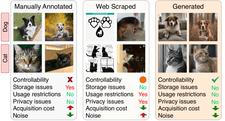
Figure 1: Generated data addresses various constraints associated with web scraping or manually annotated data, effectively mitigating privacy concerns and usage restrictions, which refers to whether images can be used for learning. Simultaneously, it maintains controllability, which encompasses the ability to generate or acquire images with various contexts (e.g., background, color) as desired. Generated data is less noisy than web-scrapped data and proves to be a more cost-effective acquisition method than manually annotated data which requires human annotation.

In CL evaluation, the prevalent assumption is that training and test data adhere to independent and identically distributed (i.i.d.) principles. However, this assumption may not hold in real-world scenarios. In the case of training a model for autonomous driving, the available data may not cover all operational domains, leading to disparities between the trained and encountered domains post-deployment [80, 126]. Therefore, we suggest evaluating performance not only within the in-distribution (ID) domain (i.e., the seen domain) but also across the out-of-distribution (OOD) domain (i.e., the unseen domain).

To this end, encompassing the integration of generated data within the online CL framework, we aim to address the following specific research questions, thereby succinctly summarizing our core contributions.

1. Is it possible for generated data to substitute manually annotated (MA) or web-crawled data in continual learning environments? To demonstrate the effectiveness of generated data, we compared the performance of G-NoCL against the training with web-scraped or MA data. This assessment spans the in-distribution (ID) and out-of-distribution (OOD) domains in online CL, using domain generalization benchmarks. E.g., employing DISCOBER results in a 9% and 10% improvement in $A_{\text{AUC}}$ on the PACS [144] OOD domain compared to the use of MA and web-scraped data for training, respectively.

2. How to ensure high-quality and diverse generated images? Within the G-NoCL framework, we incorporate a prompt refinement module $\psi$ that leverages Language Models (LLMs) to generate a diverse array of fine-grained prompts. These prompts are subsequently employed for data generation in diverse settings and contexts. We illustrate the advantages of this approach by contrasting it with the use of a single base prompt for the entire volume of data generation across online continual learning benchmarks.

3. What is the most effective approach for ensembling sampled data from various generators? We introduce a novel ensembling technique guided by data complexity, denoted as DISCOBER. This technique assesses the difficulty of samples for each concept generated by individual generators, determining appropriate weights for their contributions to the ensemble. Our investigation yields two notable findings on sample hardness and previously unexplored aspects of generators.

   • Varying generators generate samples of distinct hardness even when presented with identical prompts for a fixed concept.

   • Leveraging concept-wise harder generated samples, determined by the relative Mahalanobis distance (RMD) score [30], yields superior performance in both the ID and the OOD domains.

2 Related Work

2.0.1 Continual learning methods.

To prevent catastrophic forgetting, various continual learning methods have been proposed, and they can be categorized as follows: regularization-based, architecture-based, and replay-based methods.

Regularization-based methods [62, 139, 2, 69] prevent forgetting past tasks by regularizing important parameters to adapt to changes in subsequent tasks. Although these methods perform well in task incremental learning, they often fail to achieve good performance in more challenging setups, such as class incremental learning [4].

Architecture-based methods [143, 71, 137, 28] involve expanding parameters when learning new tasks, effectively preventing forgetting by preserving the model parameters learned for previous tasks. However, a drawback emerges as the number of parameters increases with each new task, leading to an increase in the costs of memory and computation for training [143, 81].

Replay-based methods [99, 11, 64, 125, 136, 46] store a portion of the data from previous tasks in episodic memory and are used for future tasks training to avoid forgetting previous tasks. The replay-based method demonstrates superior performance compared to alternative approaches, but causes data privacy problems due to data storage [110, 114, 130, 3, 21]. To address this problem, several studies [110, 94, 145] propose the use of generative models for replay. However, they assume that the incoming stream data are well-curated annotated data.

2.0.2 Domain generalization.

In contrast to domain adaptation, which aims to alleviate domain shift between target domains and a source domain using data from the target domain, domain generalization focuses on improving the generalizability of the model in entirely new target domains [127]. Although domain adaptation and incremental learning methods [101, 61, 128, 89] have been proposed to adapt to new domains and achieve high performance, they often involve long periods of adaptation [74].

Since long periods of adaptation are not suitable for scenarios with sudden domain shifts [74], such as autonomous driving,  [113] focus on improving the generalization performance of the unseen domain with a class-incremental setup. However, they assume the use of well-curated annotated data for new classes from various domains to enhance domain generalization abilities. Meanwhile, in the real world, there are limitations in obtaining high-quality real-time data when the concept to be learned is given.

2.0.3 Learning from models.

With the accessibility of robust generative models [100, 33, 98, 142, 13, 52, 55, 42, 56, 51, 120, 58, 92], several recent studies have investigated the potential of leveraging synthetic data for training purposes [123, 7, 36, 67, 141, 124, 78, 79]. In particular, [123] recently showcased the positive influence of employing diffusion model-generated datasets on ImageNet [32] scale for training.

Leveraging Large Language Models (LLMs) like ChatGPT [17] for CLIP [96]-based training significantly improves performance [123], suggesting generative models improve model training workflows.[141] introduces a framework to augment small datasets through conditional guided data generation using image-generative models, yet the focus remains on supervised learning, overlooking exploration in a sequential training regime where distribution shift is common.

3 Generated vs. Web-scraped Data

In modern deep learning, the trajectory of advancement is heavily influenced by the exponential growth of training data and the corresponding models trained on these vast datasets. Foundation models are typically exposed to datasets in the order of billions during training, obtained predominantly through web scraping [19, 106, 135, 146, 40, 63, 8]. Although web scraping is a cost-effective method to produce high-quality datasets, studies underscore issues such as potential biases [38, 88, 22], copyright, privacy, and license concerns [95, 116], and the risks of data contamination [31, 72] or data leakage from evaluation [9].

Previous works [117, 131, 116, 76] have emphasized the existence of sensitive individual-specific data in web-scraped or online-collected datasets, particularly in consent-driven domains such as facial images [87, 82]. Legal scrutiny and concerns about the use of such data in model training have been subject to investigation [59]. The practice of training models on large-scale web-scraped datasets has drawn attention due to potential explicit samples [132, 122] and instances of demonstrated data poisoning [23].

Recognizing the numerous issues associated with the use of web-scraped datasets, efforts have been made to ensure the fair development and utilization of foundation models [48] trained on such datasets. However, persistent challenges remain, posing substantial risks on both the legal and privacy fronts.

Generative foundation models trained on extensive web data gain efficacy when subsequent models leverage data generated by them. This approach helps overcome challenges of direct webly-supervised training. Specifically, the use of generated facial images [54, 25] has been shown to be effective for facial attribute recognition, adhering to consent and privacy terms. Harnessing the compositional generation of these models facilitates diverse dataset creation, as illustrated in Fig. 3. For fine-grained concepts and data imbalance in web queries, generative models offer a solution, as seen in prior studies [43, 53, 111, 129]. Despite the challenges in generative models, including quality concerns and social impact [57], their advantages outweigh webly-supervised drawbacks.

4 Approach

In contrast to previous works that assumed the abundance of well-curated annotated data, we explore the problem setup of online continual learning in which only new concepts are streamed to the learner $f_{\theta}$ without any data. Our aim is to address the absence of data by proposing an online, name-only continual learning framework, named G-NoCL. The G-NoCL framework is composed of four integral components: (i) the Prompt Refiner Module $\psi$ (Sec. 4.1), (ii) a set of Generators $\mathcal{G}$ (Sec. 4.2), (iii) a Ensembler represented by $\Delta$ (Sec. 4.3), and (iv) the learner $f_{\theta}$.

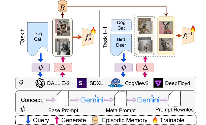
Figure 2: G-NoCL framework: In an online CL setting, the learner $f_{\theta}$ receives new concepts which is passed through a prompt refiner module $\psi$ to obtain fine-grained prompts. These prompts are subsequently used to generate data from the set of generators $\mathcal{G}$ which is used for training of $f_{\theta}$. In addition, we maintain a episodic memory with finite size $B$.

When a new concept is introduced, for which $f_{\theta}$ needs to be learned, a generator $g\in\mathcal{G}$ generates images related to the given concept. However, generative models have limitations in terms of the finite diversity of their output [75, 104]. Therefore, we try to maximize the output diversity of the generative model through the Prompt Refiner Module $\psi$. Furthermore, to enhance the diversity of generated images, we employ an ensemble approach by combining the outputs of a set of generators ${\mathcal{G}}$ through a complexity-aware ensembler $\Delta$.

As the images are generated, they are promptly streamed in real-time to the learner $f_{\theta}$. Simultaneously, a finite episodic memory is maintained to replay previously encountered data. One thing to note here is that, unlike real data, such as web-scraped data, the method of storing samples in episodic memory is free from data privacy issues. While it is possible to generate data for past concepts in real-time without using memory, we use it for efficiency, as it allows for reducing computational costs without privacy concerns.

4.1 Prompt Refiner Module $\psi$

Given new concepts, we pass them through the prompt refiner module $\psi$. The pipeline $\psi$, as indicated in Fig. 2, takes the new concept as input and then constructs the base prompt. For the base prompt, we use the template: "This is an image of the [concept]", following [112, 108]. While this base prompt can serve as input for generators $\mathcal{G}$, generating a large number of images using the same prompt may result in limited diversity in terms of style, texture, and background elements in the generated images. So, we feed the base prompt into a language model (LLM), namely the Gemini model [121], to generate a series of meta-prompts, taking advantage of the in-context learning capability inherent in LLMs [17, 123].

We initially generate 10 meta-prompts based on different variations of style, background, and tone. For example, within the style category, one of the meta-prompts that we obtained was: "A minimalist image of [concept] using clean lines and muted colors". After obtaining the meta-prompts, we prompt Gemini [121] again to rewrite each of the meta-prompts in four different ways, thus creating a total set of 50 prompts. An example prompt-rewrite for the prompt provided above was "Minimalist composition of [concept] with clean lines and a subdued color palette". Note that we use the rewritten prompt without any selection and do not include domain-specific information in the prompt. Please refer to the supplementary material for more details on the meta-prompts used and the subsequent prompt rewrites generated.

4.2 Generators $\mathcal{G}$

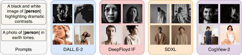
Figure 3: Examples of PACS [144] generated samples from various generators using two of the prompt rewrites. Illustrations from the concept "Person" are showcased.

We augmented the diversity of generated samples by a single model through the utilization of a range of diversified prompts, denoted as intra-diversity. Additionally, we sought to amplify the inter-diversity by incorporating various text-to-image (T2I) generative models. Concretely, we establish a set of generators ${\mathcal{G}}$ predominantly based on four distinct T2I generators: (i) Stable Diffusion XL [92], (ii) DALL.E-2 [13], (iii) CogView2 [33], and (iv) DeepFloyd IF. As illustrated in Figure 3, different generators produce varied samples when prompted with identical prompts conditioned on the same concept.

4.3 Ensembler $\Delta$

We increase the inter-diversity of generated images by using various T2I models together. Here, a question arises: When ensembling images generated by different T2I models, which images should be included? One of the naive yet intuitive ensemble methods is to mix images generated by each generator with equal weights. However, considering the potential existence of similar images among those generated by each generative model, it is better to mix them in a way that minimizes overlap rather than to ensemble them with the same ratio to increase inter-diversity.

Therefore, we focus on ensembling samples positioned far from the class prototype in the feature space, indicating those that are challenging to classify, rather than close to the prototype, which are easily identifiable. To identify such samples, we use the relative Mahalanobis distance (RMD) [30] score, which measures the difficulty of classifying a sample into a corresponding class by comparing the distance from the class prototype to the distance from the global prototype. The RMD score for a sample $(x_{i},y_{i})$ is given by the following:

$$\mathcal{RMD}(x_{i},y_{i})=\mathcal{M}(x_{i},y_{i})-\mathcal{M_{\mathrm{agn}}}(x_{i}),$$ (1)

where $\mathcal{M}(x_{i},y_{i})$ refers to the Mahalanobis distance [68] between a sample $x_{i}$ and its class prototype, while $\mathcal{M_{\mathrm{agn}}}(x_{i})$ refers to the distance to the global prototype. The class prototype is obtained from the average features within a class, computed using a frozen CLIP [96] image encoder, representing its most representative features. On the contrary, the global prototype is computed from the average features across all classes.

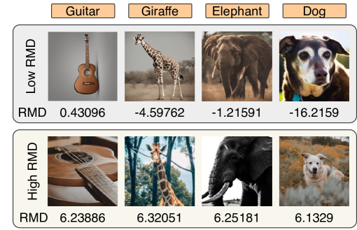
(a)

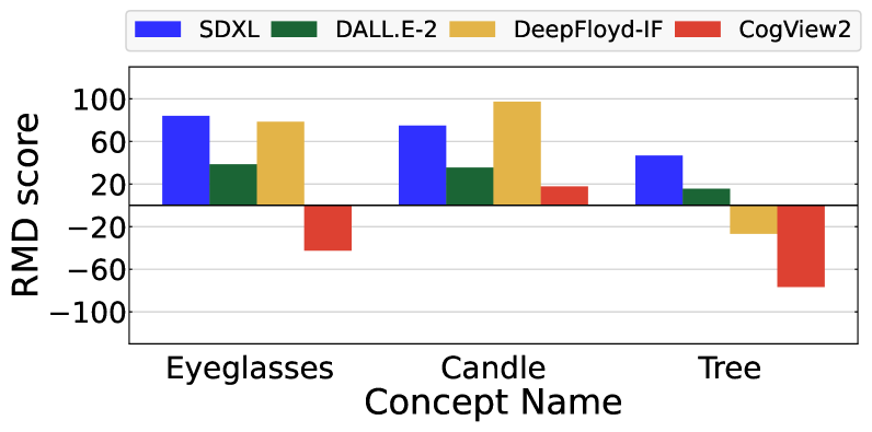
(b)

Figure 4: (a) - Examples of samples with a high RMD score and a low RMD score, (b)-Concept-wise RMD score distributions for generated images by each generative model

If the distance from the class prototype is close and the distance from the global prototype is far, leading to a low RMD score, the sample can be considered to be easy to classify into the ground truth class. Conversely, if the distance from the class prototype is far and close to the global prototype, resulting in a high RMD score, it is more likely to be classified not only as the ground truth class but also as another class, i.e., the sample can be considered difficult. We show samples with low RMD scores and samples with high RMD scores in Fig. 4-(a).

In online CL, where data encounters in a streaming manner, we continuously update class and global prototypes using a simple moving average and a simple moving variance [6]. For more details on the calculation of the RMD score in the online CL setup, please refer to the supplementary material.

By using the RMD score, we can ensemble images that are difficult to classify, which are expected to exhibit a widespread dispersion from the class prototype. However, in the coreset, which is a representative subset of an entire dataset [5], it is necessary to include not only samples near the decision boundary, but also class-representative samples [11, 45].

Therefore, we use a probabilistic approach to ensemble selection, rather than just selecting images with the $k$-highest RMD scores. Since the diversity of generated images varies across generators for each individual class, as shown in Fig. 4-(b), we calculate a class-specific selection probability for each generator $g\in\mathcal{G}$, denoted as $p_{g|c}$ as follows:

$$p_{g|c}=\frac{e^{\overline{RMD}_{g|c}/T}}{\sum_{h\in\mathcal{G}}e^{\overline{RMD}_{h|c}/T}},$$ (2)

where $\overline{RMD}_{g|c}$ is the average RMD score of the samples generated by the generator $g$ for class $c$. By adjusting model selection based on class-specific RMD scores, we enhance the diversity of the ensemble, ensuring that the ensemble includes samples that are difficult to classify.

We substantiate our hypothesis through empirical validation in a comparative study using various RMD-based ensembles, as presented in Table 1. The table reveals that, with the exception of DISCOBER, all ensemble methods exhibit a decrease in performance compared to the scenario where no ensembling is applied. DISCOBER demonstrates a notable performance advantage over the others in both In-Distribution (ID) and Out-of-Distribution (OOD) evaluations. The $k$-highest RMD ensemble, which excludes easy samples, leads to insufficient learning in the class-representative region, while the $k$-lowest RMD concentrates solely on easy samples, resulting in limited diversity. Inverse DISCOBER employs the inverse of the probabilities utilized in DISCOBER. Similar to the $k$-lowest RMD ensemble, it tends to prioritize easy samples, leading to a decline in performance.

Table 1: Comparison of ensemble methods in PACS [144], using DER [18] for all ensemble methods. The proposed ensemble method outperforms other ensemble methods.

Ensemble Method $\Delta$	ID		OOD
	$A_{\text{AUC}}\ \uparrow$	$A_{last}\ \uparrow$	$A_{\text{AUC}}\ \uparrow$	$A_{last}\ \uparrow$
None (Baseline)	47.34$\pm$2.64	44.64$\pm$3.08	31.33$\pm$1.71	25.36$\pm$1.31
Equal weight ensemble	43.39$\pm$2.01	36.32$\pm$2.76	29.77$\pm$1.74	21.47$\pm$1.73
$k$-highest RMD ensemble	50.13$\pm$1.99	41.60$\pm$3.79	31.28$\pm$1.23	26.66$\pm$1.46
$k$-lowest RMD ensemble	31.16$\pm$0.87	21.60$\pm$2.66	25.45$\pm$1.56	11.95$\pm$1.33
Inverse Prob	40.48$\pm$1.72	23.74$\pm$0.97	27.98$\pm$0.91	20.13$\pm$1.37
DISCOBER (Ours)	50.22$\pm$2.41	45.10$\pm$1.69	32.77$\pm$1.62	28.78$\pm$1.49

5 Experiments

5.1 Baselines

To investigate the effectiveness of using generative models in the name-only CL setup, we performed experiments using various CL methods, and these methods can be broadly categorized into three categories: Replay-based method (ER [99], DER [18], ASER [109], MIR [3], and X-DER [16]), Regularization-based method (LiDER [15]), and Architecture-based method (MEMO [143]). For more details about the baselines, please refer to the supplementary material.

5.2 Experimental Setup

5.2.1 Datasets.

Table 2: Split of in-distribution (ID) domain and out-of-distribution (OOD) domain for each domain generalization benchmark.

Dataset	ID domain	OOD domain
PACS [144]	Photo	Art, Cartoon, Sketch
DomainNet [83]	Real	Clipart, Painting, Sketch
CIFAR-10-W [118]	-	CIFAR-10-W [118]
CCT [12]	10 locations	10 other locations

To measure domain generalization performance, we used widely used domain generalization benchmarks: PACS [144] and DomainNet [83]. For each benchmark, only the training set of one domain was used as manually anotated (MA) data, and the other domain data were used as out-of-distribution (OOD) test domain. The performance of the in-distribution (ID) domain was evaluated using the test set of the domain used for training, while the OOD performance was evaluated using data from the remaining domains (i.e., domains not used for training). We also used CIFAR-10-W [118] and CCT [12] to evaluate the performance of domain generalization. CIFAR-10-W is a dataset collected by scraping data from the Web, covering the same classes as the well-known CIFAR-10 dataset [66], and is composed of instances from cartoon and non-cartoon domains. Since it consists of only two domains, both are used to evaluate the out-of-distribution (OOD) domain. As CIFAR-10-W is a web-scraped dataset, the domain of CIFAR-10-W and the web-scraped data are the same. Therefore, we excluded web-scraped data in experiments on CIFAR-10-W. CCT [12] is a subsampled dataset from Terra Incognita [12], a collection that captures images of animals in various fixed locations. The CCT dataset comprises data collected from a total of 20 locations. For more details on the experiment setup, please refer to the supplementary material. We summarize the ID and OOD domain for each dataset in Tab. 2.

5.2.2 Metrics.

We addressed a name-only online Continual Learning (CL) scenario where, upon presenting a given concept for learning, the model is trained using the generated data streamed in real time. In such an online CL setup, the model is used for inference at every moment rather than the predefined time point (e.g., end of the task) [64, 20, 10, 91]. Therefore, to measure the inference performance at any time, we evaluated the model at regular intervals during a specified evaluation period and then calculated the area under the accuracy curve, denoted $A_{\text{AUC}}$ [64, 20, 65]. Furthermore, we used $A_{last}$ to evaluate the performance of the model at the end of the training.

Table 3: In distribution (ID) domain and out-of-distribution (OOD) domain accuracy of CL methods when the names of PACS and DomainNet data are given incrementally. We use ResNet-18 as the backbone architecture. We followed the ID and OOD domains as described in the Tab. 2. As detailed in Sec. 4.1, we use "An image of [concept name]" as our base prompt. The term Gen. Ensemble denotes the generator ensemble, which encompasses the Diversified Prompt, i.e., the result of Gen. Ensemble corresponds to the result of DISCOBER.

Method	Training Data	PACS				DomainNet
		ID		OOD		ID		OOD
		$A_{\text{AUC}}\ \uparrow$	$A_{last}\ \uparrow$	$A_{\text{AUC}}\ \uparrow$	$A_{last}\ \uparrow$	$A_{\text{AUC}}\ \uparrow$	$A_{last}\ \uparrow$	$A_{\text{AUC}}\ \uparrow$	$A_{last}\ \uparrow$
ER [99]	Web-scraped	53.08$\pm$2.73	50.91$\pm$2.57	29.01$\pm$2.17	24.70$\pm$0.83	31.98$\pm$0.38	23.29$\pm$0.22	9.97$\pm$0.23	6.97$\pm$0.13
	Base Prompt	46.33$\pm$1.75	45.34$\pm$3.60	27.96$\pm$1.69	20.47$\pm$1.39	25.13$\pm$0.38	21.38$\pm$0.71	7.28$\pm$0.15	5.29$\pm$0.13
	(+) Diversified Prompt	47.95$\pm$2.20	45.58$\pm$3.00	34.11$\pm$1.33	27.13$\pm$1.69	25.23$\pm$0.31	20.72$\pm$0.35	9.15$\pm$0.26	7.35$\pm$0.04
	(+) Gen. Ensemble	53.83$\pm$2.96	51.68$\pm$2.68	35.69$\pm$1.62	30.09$\pm$1.42	28.52$\pm$0.07	24.02$\pm$0.86	11.42$\pm$0.04	9.67$\pm$0.47
	Manually Annotated	70.21$\pm$3.71	72.11$\pm$1.57	28.53$\pm$1.81	22.08$\pm$1.31	48.56$\pm$0.23	40.22$\pm$0.55	12.68$\pm$0.10	10.19$\pm$0.18
ER-MIR [3]	Web-scraped	47.45$\pm$4.47	44.57$\pm$5.26	27.97$\pm$2.20	18.17$\pm$1.55	32.39$\pm$0.31	23.36$\pm$0.32	10.25$\pm$0.23	7.26$\pm$0.07
	Base Prompt	49.34$\pm$2.11	46.71$\pm$0.83	28.24$\pm$1.56	21.00$\pm$2.16	24.81$\pm$0.43	21.17$\pm$0.32	7.23$\pm$0.22	5.73$\pm$0.15
	(+) Diversified Prompt	50.46$\pm$2.18	49.62$\pm$3.43	34.36$\pm$1.82	28.02$\pm$1.16	24.82$\pm$0.20	20.56$\pm$0.35	9.10$\pm$0.20	7.51$\pm$0.15
	(+) Gen. Ensemble	54.28$\pm$3.84	55.31$\pm$1.05	37.42$\pm$1.80	33.90$\pm$0.93	28.36$\pm$0.13	23.74$\pm$0.37	11.43$\pm$0.10	9.59$\pm$0.19
	Manually Annotated	68.15$\pm$5.06	70.98$\pm$1.98	28.78$\pm$2.26	21.14$\pm$1.04	49.20$\pm$0.10	40.54$\pm$0.46	12.96$\pm$0.03	10.33$\pm$0.25
DER++ [18]	Web-scraped	48.39$\pm$3.17	36.50$\pm$4.24	26.89$\pm$1.86	18.88$\pm$1.00	32.09$\pm$0.36	22.37$\pm$0.42	9.92$\pm$0.20	6.42$\pm$0.04
	Base Prompt	41.47$\pm$2.26	39.41$\pm$2.90	27.74$\pm$1.41	18.82$\pm$1.57	26.64$\pm$0.39	22.04$\pm$0.37	7.91$\pm$0.24	5.85$\pm$0.05
	(+) Diversified Prompt	47.34$\pm$2.64	41.60$\pm$4.08	32.33$\pm$1.71	25.36$\pm$1.31	25.61$\pm$0.36	20.06$\pm$0.38	9.40$\pm$0.13	7.20$\pm$0.17
	(+) Gen. Ensemble	49.02$\pm$2.41	45.10$\pm$1.69	33.07$\pm$1.62	28.78$\pm$1.49	29.67$\pm$0.06	23.37$\pm$0.38	11.89$\pm$0.02	9.41$\pm$0.16
	Manually Annotated	63.90$\pm$5.04	61.19$\pm$2.92	27.49$\pm$1.77	19.75$\pm$1.58	49.35$\pm$0.33	39.40$\pm$0.20	12.62$\pm$0.13	9.27$\pm$0.18
ASER [109]	Web-scraped	49.12$\pm$3.32	42.49$\pm$4.06	27.50$\pm$1.92	19.04$\pm$1.48	33.80$\pm$0.38	23.09$\pm$0.84	9.80$\pm$0.51	6.43$\pm$0.69
	Base Prompt	40.35$\pm$1.25	38.04$\pm$2.79	26.64$\pm$1.28	18.06$\pm$0.80	25.42$\pm$0.24	22.93$\pm$0.19	7.71$\pm$0.64	5.13$\pm$0.76
	(+) Diversified Prompt	48.28$\pm$0.67	45.40$\pm$2.95	33.76$\pm$1.20	25.48$\pm$1.94	25.94$\pm$0.26	20.93$\pm$0.31	9.87$\pm$0.02	5.64$\pm$0.44
	(+) Gen. Ensemble	48.38$\pm$1.95	47.24$\pm$2.07	35.07$\pm$1.46	31.58$\pm$2.09	32.01$\pm$0.85	24.28$\pm$0.70	11.56$\pm$0.62	8.25$\pm$0.98
	Manually Annotated	68.00$\pm$4.95	70.33$\pm$2.58	26.81$\pm$1.72	19.21$\pm$1.16	48.92$\pm$0.43	40.93$\pm$0.12	10.51$\pm$1.27	6.43$\pm$0.12
MEMO [143]	Web-scraped	49.27$\pm$2.52	39.88$\pm$4.93	28.00$\pm$1.53	19.19$\pm$1.36	30.17$\pm$0.25	21.40$\pm$0.24	9.29$\pm$0.27	6.28$\pm$0.03
	Base Prompt	43.67$\pm$0.90	39.76$\pm$4.72	27.22$\pm$1.09	17.00$\pm$0.67	23.54$\pm$0.32	19.45$\pm$0.22	6.82$\pm$0.16	4.98$\pm$0.05
	(+) Diversified Prompt	48.80$\pm$1.69	46.59$\pm$2.50	32.21$\pm$1.55	24.56$\pm$0.47	23.59$\pm$0.22	19.30$\pm$0.30	8.63$\pm$0.11	6.83$\pm$0.11
	(+) Gen. Ensemble	50.20$\pm$2.37	48.72$\pm$0.91	33.50$\pm$1.36	29.43$\pm$2.79	26.88$\pm$0.35	21.67$\pm$0.20	10.61$\pm$0.13	8.58$\pm$0.19
	Manually Annotated	67.37$\pm$4.67	66.94$\pm$2.26	27.73$\pm$1.59	20.63$\pm$0.71	47.04$\pm$0.43	38.25$\pm$0.45	11.77$\pm$0.20	8.99$\pm$0.26
X-DER [16]	Web-scraped	50.44$\pm$2.93	41.96$\pm$2.11	27.57$\pm$1.78	20.73$\pm$1.06	31.68$\pm$0.21	23.00$\pm$0.95	10.93$\pm$0.44	8.54$\pm$0.10
	Base Prompt	44.78$\pm$2.77	46.59$\pm$2.62	29.86$\pm$1.63	22.86$\pm$0.99	27.41$\pm$0.23	24.11$\pm$0.85	7.91$\pm$0.65	6.65$\pm$0.12
	(+) Diversified Prompt	49.68$\pm$2.97	46.94$\pm$3.53	33.61$\pm$2.07	24.74$\pm$2.70	26.72$\pm$0.75	21.71$\pm$0.43	9.28$\pm$0.86	7.65$\pm$0.39
	(+) Gen. Ensemble	50.52$\pm$1.57	48.19$\pm$2.47	33.69$\pm$1.36	26.73$\pm$0.54	32.14$\pm$0.52	25.48$\pm$0.16	12.39$\pm$0.74	10.04$\pm$0.54
	Manually Annotated	66.19$\pm$4.78	68.49$\pm$1.85	28.61$\pm$1.92	20.54$\pm$0.81	50.35$\pm$0.20	42.41$\pm$0.14	12.99$\pm$0.29	10.68$\pm$0.83
LiDER [15]	Web-scraped	51.07$\pm$3.06	44.69$\pm$2.22	27.95$\pm$1.60	22.16$\pm$1.22	30.95$\pm$0.34	23.55$\pm$0.28	9.93$\pm$0.20	7.25$\pm$0.08
	Base Prompt	45.73$\pm$2.65	43.26$\pm$4.86	29.24$\pm$1.30	22.12$\pm$1.07	24.27$\pm$0.20	21.29$\pm$0.45	7.05$\pm$0.08	5.55$\pm$0.06
	(+) Diversified Prompt	51.74$\pm$2.48	51.40$\pm$2.79	34.04$\pm$1.90	27.10$\pm$1.41	24.55$\pm$0.10	20.78$\pm$0.39	9.05$\pm$0.16	7.56$\pm$0.14
	(+) Gen. Ensemble	52.46$\pm$3.11	52.35$\pm$3.26	36.18$\pm$1.44	30.94$\pm$1.24	30.09$\pm$0.41	24.04$\pm$0.32	11.42$\pm$0.34	9.26$\pm$0.29
	Manually Annotated	66.31$\pm$5.69	66.59$\pm$2.60	29.11$\pm$2.19	21.21$\pm$1.03	47.75$\pm$0.16	40.06$\pm$0.35	12.34$\pm$0.09	10.06$\pm$0.08

5.2.3 Implementation Details.

We used ResNet-18 [47] and Vision Transformer (ViT) [34] as network architectures for all datasets. Due to the large number of parameters in ViT, training it from scratch in an online setup resulted in lower performance. Therefore, we used the weights of a model pre-trained on ImageNet-1K [102] as initial weights for ViT. For data augmentation, we consistently applied RandAugment [29] across all datasets and CL methods.

Following [64, 65, 60], we conduct batch training for each incoming sample. Specifically, for PACS, CCT, CIFAR-10-W, and DomainNet, the number of batch iterations per incoming sample is set to 2, 2, 2, and 3, respectively, with batch sizes of 16, 16, 16, and 64. Episodic memory sizes are configured as 200, 400, 1000, and 8000 for PACS, CCT, CIFAR-10-W, and DomainNet, respectively. To ensure a fair comparison among manually annotated data, generated data, and web-scraped data, we used an equal number of samples in all experiments. Regarding the web-scraped data, we obtained 20% more samples than necessary for batch training with the aim of filtering out noisy data. To achieve this, we utilized pre-trained CLIP [96] for filtering, which excludes the most noisy bottom samples, resulting in a cleaned subset used for training, following [106].

In all experiments, we run five different random seeds and report the average and standard error mean. For the class-incremental setup, we adopt a disjoint configuration, where tasks do not share classes [90]. We employ the Gemini model [121], a Large Language Model, to generate diverse meta-prompts. On manual inspection, Gemini exhibits superior performance in producing well-structured meta-prompts compared to ChatGPT [17].

5.3 Results

Table 4: Comparison of Manually Annotated (MA) data and DISCOBER on CIFAR-10-W. We use ResNet-18 as the backbone.

Method	Training Data	$A_{\text{AUC}}\ \uparrow$	$A_{last}\ \uparrow$
ER	DISCOBER	60.93$\pm$3.92	48.20$\pm$0.27
	MA	48.97$\pm$0.56	31.27$\pm$2.31
ER-MIR	DISCOBER	58.19$\pm$0.86	46.01$\pm$0.34
	MA	44.77$\pm$0.86	35.01$\pm$2.50
DER++	DISCOBER	53.88$\pm$1.22	39.53$\pm$1.42
	MA	45.25$\pm$0.07	28.75$\pm$1.44
ASER	DISCOBER	54.34$\pm$0.66	41.88$\pm$1.00
	MA	50.00$\pm$0.59	34.86$\pm$1.17
MEMO	DISCOBER	53.59$\pm$0.67	41.69$\pm$0.67
	MA	45.40$\pm$0.56	30.97$\pm$2.13
X-DER	DISCOBER	57.56$\pm$0.75	45.97$\pm$0.17
	MA	47.14$\pm$0.82	33.41$\pm$1.34
LiDER	DISCOBER	57.13$\pm$0.29	45.41$\pm$2.58
	MA	46.97$\pm$0.42	28.79$\pm$4.27

To assess whether our proposed method works well in a setup where only class names are provided without data, we compare it with the scraped data from the Web. Additionally, we compare the performance when manually annotated data are provided as an ideal case. We summarize the results not only in the ID domain but also in the OOD domain in Tab. LABEL:tab:cct_pacs_resnet, Tab. 4, and Tab. LABEL:tab:cct_pacs_vit.

In-distribution (ID) domain evaluation uses the test set of manually annotated (MA) data. Hence, we anticipate that the model trained using manually annotated (MA) data will establish an upper performance bound, showcasing superior results in comparison. However, interestingly, in the out-of-distribution (OOD) domain of PACS, DISCOBER outperforms not only MA data but also web-scraped data. We believe that we achieve better generalization performance by generating a more diverse set of images through a diversified set of prompts and an ensemble of generators. One thing to note here is that DomainNet is a benchmark created through web scraping, resulting in a domain overlap with web data. Despite this, DISCOBER outperforms the web-scraped data in DomainNet.

CCT is a domain-specific benchmark captured by fixing cameras at various locations in the wild, including photos taken at night or obscured by natural elements such as trees or rocks. Therefore, although photos taken at different locations are categorized as OOD in CCT, OOD data include a substantial number of images resembling the ID domain, in contrast to web-scraped or generated data. Due to these domain-specific characteristics, models trained on MA data in CCT exhibit superior performance across both ID and OOD domains compared to models trained on web-scraped or generated data. When evaluating the performance of models trained on web-scraped data against data generated using DISCOBER in CCT, DISCOBER demonstrates superior performance in both ID and OOD domains.

In summary, we explore the G-NoCL setup where only the concept names that learners need to learn are provided. When exclusively trained on images generated using DISCOBER, without relying on any human-annotated MA data, we achieved the best performance in the OOD domains of all benchmarks (i.e., PACS, CCT, CIFAR-10-W, and DomainNet) with which we experimented. Additionally, compared to web-scraped data, our approach outperforms ID domain accuracy in the majority of benchmarks, excluding some ID domains, and consistently outperforms OOD domain accuracy across all benchmarks we used.

Table 5: In distribution (ID) domain and out-of-distribution (OOD) domain accuracy of CL methods when the names of PACS and CCT data are given incrementally. We use ViT [103] as the backbone architecture. We followed the ID and OOD domains as described in the Tab. 2. MA denotes manual annotations.

Method	Training Data	PACS				CCT
		ID		OOD		ID		OOD
		$A_{\text{AUC}}\ \uparrow$	$A_{last}\ \uparrow$	$A_{\text{AUC}}\ \uparrow$	$A_{last}\ \uparrow$	$A_{\text{AUC}}\ \uparrow$	$A_{last}\ \uparrow$	$A_{\text{AUC}}\ \uparrow$	$A_{last}\ \uparrow$
ER [99]	Web-scraped	47.12$\pm$4.67	30.51$\pm$5.98	29.78$\pm$1.90	15.71$\pm$1.94	24.98$\pm$1.02	11.00$\pm$0.90	21.71$\pm$0.75	9.93$\pm$0.78
	DISCOBER	55.25$\pm$4.11	48.84$\pm$3.95	33.24$\pm$1.62	23.14$\pm$1.21	25.50$\pm$0.99	12.03$\pm$0.81	25.16$\pm$0.56	14.13$\pm$0.95
	Manually Annotated	72.93$\pm$5.29	70.51$\pm$1.75	30.68$\pm$1.95	20.85$\pm$0.84	52.20$\pm$2.52	$34.07\pm$3.41	42.29$\pm$1.55	22.10$\pm$2.13
ER-MIR [3]	Web-scraped	48.78$\pm$5.96	40.95$\pm$5.92	28.71$\pm$2.24	20.03$\pm$3.24	23.07$\pm$3.31	12.37$\pm$2.78	22.64$\pm$2.43	12.20$\pm$4.23
	DISCOBER	50.74$\pm$4.09	51.51$\pm$1.83	31.84$\pm$1.93	25.17$\pm$1.05	23.72$\pm$0.18	12.59$\pm$0.65	24.82$\pm$0.34	14.01$\pm$4.83
	Manually Annotated	68.21$\pm$6.44	73.29$\pm$1.90	28.69$\pm$1.96	23.03$\pm$0.85	37.75$\pm$1.36	18.99$\pm$1.43	33.38$\pm$0.70	15.31$\pm$1.27
DER++ [18]	Web-scraped	53.61$\pm$3.39	45.71$\pm$4.20	27.66$\pm$1.46	18.75$\pm$1.63	23.19$\pm$0.51	9.17$\pm$1.11	22.17$\pm$0.60	8.93$\pm$0.66
	DISCOBER	50.44$\pm$4.32	43.96$\pm$3.32	30.30$\pm$1.81	20.91$\pm$0.86	25.24$\pm$1.28	10.63$\pm$0.85	24.39$\pm$0.92	10.17$\pm$0.73
	Manually Annotated	64.81$\pm$6.75	61.36$\pm$2.37	28.94$\pm$2.03	19.95$\pm$1.64	44.05$\pm$2.67	19.50$\pm$2.78	38.02$\pm$1.18	17.10$\pm$2.21
ASER [109]	Web-scraped	56.32$\pm$5.10	49.55$\pm$4.53	30.67$\pm$2.58	21.82$\pm$2.04	25.48$\pm$1.05	12.84$\pm$1.40	22.33$\pm$0.85	12.23$\pm$0.99
	DISCOBER	56.06$\pm$4.60	52.04$\pm$3.85	33.99$\pm$2.02	25.81$\pm$0.92	26.15$\pm$1.74	13.97$\pm$1.04	24.85$\pm$1.13	12.73$\pm$1.36
	Manually Annotated	77.83$\pm$7.77	76.48$\pm$9.23	43.37$\pm$4.28	35.87$\pm$7.47	54.28$\pm$1.71	47.67$\pm$1.85	45.07$\pm$1.56	28.07$\pm$0.72

5.4 Ablation Study

We conduct an ablation study on two components of DISCOBER, namely the diversified prompt and generator ensemble, and summarize the results in Tab. LABEL:tab:cct_pacs_resnet. Our observations indicate that both the diversified prompt and generator ensemble play a significant role in enhancing not only the ID domain performance but also the OOD domain performance.

5.5 Scaling behavior

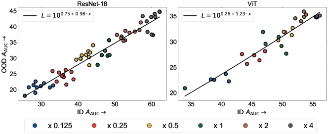
Figure 5: Ensemble scaling behavior of (a) ResNet-18 [47] and (b) ViT [34] for ID $A_{\text{AUC}}$ vs. OOD $A_{\text{AUC}}$ on the PACS dataset [144] using ER [99]. (x 1) denotes the ensemble volume in primary experiments, the default data budget.

Recent scaling law studies [49, 50] offer predictive insight into model performance by scaling computation, data, and model capacity. Despite the limited exploration of scaling in continual learning settings [97], and particularly with synthetic data [35] being confined to static frameworks, our empirical analysis in Fig. 5 delves into scaling dynamics with varying generated data proportions for training online continual learners.

For ResNet-18 [47] and ViT [34], we observe a consistent linear improvement trend in both ID and OOD $A_{\text{AUC}}$ as the volume of generated data increases in the PACS [144] dataset. This scaling behavior underscores the positive correlation between performance improvement and larger, optimally curated generated data ensembles in online continual learning, reinforcing the rationale for the use of generators in the absence of annotated data.

6 Conclusion

Online continual learning represents a practical and real-world-aligned learning paradigm. However, assumptions regarding the availability of high-quality, diverse and annotated data in such scenarios lack a solid foundation. In addressing the challenges associated with training on web-crawled and manually annotated data, we introduce a unified name-only online continual learning framework that integrates generators with the continual learner, termed "Generative Name only Continual Learning" (G-NoCL).

Within the G-NoCL framework, we propose an inaugural method for prompt diversification ($\psi$) and sample complexity-guided ensembling ($\Delta$), denoted as DISCOBER. Extensive experimental evaluations demonstrate the performance improvements achieved by DISCOBER within the G-NoCL framework, showcasing its effectiveness in both in-distribution (ID) and out-of-distribution (OOD) settings compared to webly-supervised and manually annotated approaches.

6.0.1 Limitations and future work.

While DISCOBER provides a foundational strategy for optimal generator ensembling, we acknowledge limitations arising from the use of curated prompt rewrites without incorporating feedback from the continual learner. In addition, we acknowledge limitations associated with the fact that the generative model cannot produce high-quality images in all domains without fine-tuning.

In future endeavors, our aim is to expand the G-NoCL framework into multi-concept settings, leveraging and enhancing the compositional generation capabilities of T2I models. This extension encompasses broadening the proposed framework to dense prediction tasks such as semantic segmentation and object detection, and tasks in other modalities such as code generation.

Appendix 0.A Details about Experiment Setup

To set a domain generalization benchmark for a class incremental learning (class-IL) setup, we divide it into multiple disjoint tasks. Tasks do not share classes, since we assume a disjoint setup. We summarize the total number of classes per dataset, the number of classes per task, and the number of tasks in Table 6. Within each dataset, all tasks have the same size, except PACS, which has a total of 7 classes. For PACS, the first task includes 3 classes, while the subsequent tasks include data for 2 classes each.

Table 6: Task configurations for class-IL setup on each domain generalization dataset.

Dataset	total $\#$ of classes	$\#$ of tasks	$\#$ of classes / task
PACS [144]	7	3	2 (only initial task: 3)
DomainNet [83]	345	5	69
CIFAR-10-W [118]	10	5	2
CCT [12]	12	4	3

Appendix 0.B Details of Baselines

0.B.0.1 Replay-based method.

ER [99], DER [18], ASER [109], MIR [3], and X-DER [16] are methods that store previously encountered data in episodic memory and use them during future training to prevent forgetting. Since replay-based methods achieve strong performance, we chose many of them as baselines. ER, despite its simplicity, exhibits robust performance, as demonstrated in later studies[41, 107]. DER stores not only images and labels, but also logits in the form of triplets, distilling information about previous tasks through stored logits. X-DER is an extended version of DER, which addresses the logit outdated problem of DER through logit updates and future preparation. ASER and MIR retrieve training batches from episodic memory using adversarial shapely value and degree of interference, respectively, instead of random retrieval.

0.B.0.2 Regularization-based method.

LiDER [15] addresses the challenge of poor generalization in online CL due to the instability of decision boundaries, using layer-wise Lipschitz constants. LiDER is a plug-and-play method that can be combined with other CL baselines. Given that the paper that introduced LiDER demonstrated that it achieved the best performance when integrated with X-DER [16], we presented the combined results of LiDER and X-DER as the performance of LiDER.

0.B.0.3 Architecture-based method.

MEMO [143] is a network expansion approach in which the back-end layers are task-specific for each task, while the front-end layers are shared across tasks.

Appendix 0.C Manual Annotation vs. Web-Scraping vs. Generative data

As demonstrated in Fig. 1, we highlight the key differences between Manually Annotated (MA), Web scraped, and Generated data on six different axes: (a) Controllability, (b) Storage issues, (c) Usage restrictions, (d) Privacy issues, (e) Acquisition cost, and (f) Noise. In this section, we aim to provide the definition of each of these axes and their corresponding implications on each type of data source.

0.C.0.1 Controllability

encompasses the ability to generate or acquire images with various contexts, backgrounds, settings, and themes as desired. It pertains to the ability to obtain images depicting different concepts in compositions not commonly found in natural environments, as well as in domains relevant to the task at hand. Under this definition, we assert that the MA data exhibit low controllability. This limitation arises from its reliance on data captured from a finite set of scenarios or sensors, which inherently restricts the breadth of diverse settings where the concept can be observed. Web-scrapped data also suffer from low controllability for the same reasons. In contrast, the generated data have high controllability due to the ability of foundation text-to-image (T2I) generators to produce diverse images for each concept through varied prompting.

0.C.0.2 Storage issues.

Storing extensive data, locally or in the cloud, imposes additional costs, which can become impractical in environments constrained by limited total storage capacity. In addition, transmitting large, substantial data samples in a federated setup can face challenges arising from bandwidth and latency bottlenecks. In such contexts, depending on a large corpus of MA data becomes counterintuitive. On the other hand, both web-scraped and generated data present themselves as cost-effective alternatives for accessing substantial data volumes without necessitating explicit storage expenditures.

0.C.0.3 Usage restrictions

encompass limitations imposed on the utilization of images for training machine/deep learning models, typically due to copyright or licensing protections. These restrictions arise from various legal frameworks across different demographics, regulating and sometimes prohibiting the training of models on protected data for commercial deployment. This challenge is particularly prevalent in web-scraped data, where the abundance of protected data may not be adequately filtered out. On the contrary, MA data bypass this issue, as it is presumed that the data are filtered or obtained from a proprietary source with appropriate permissions during annotation. Notably, generated data offer a more advantageous position, as they do not necessitate such filtering and encounter limited or no usage restrictions, thereby providing a readily available solution to issues arising from data protection concerns.

0.C.0.4 Privacy issues

may arise when data samples inadvertently leak or explicitly contain sensitive, confidential, or private user information. Examples of such images could include those featuring people’s faces or personal objects that disclose identity-related details, such as addresses or financial assets. Once again, web data emerge as the primary source vulnerable to issues stemming from the use of private data, a topic extensively discussed in Sec. 3 of the main paper. As discussed above, MA data are expected to be protected from privacy concerns due to prior filtering or explicit agreement on data usage before annotation. In comparison, generated data should ideally not contain private data. Furthermore, several recent works [26, 27, 24, 133] have explored methods to enforce fairness and differential privacy in data synthesis, offering solutions for identity protection.

0.C.0.5 Acquisition cost

refers to the total expenses incurred in obtaining a specific number of data samples necessary to train or evaluate the learner $f_{\theta}$ for a particular task. As emphasized in 1, MA data entail a substantial acquisition cost, primarily due to the expenses associated with densely annotating the data through human workers. This, coupled with the rigorous filtering process, makes MA data prohibitively expensive to acquire at scale. Although web data do not require such significant financial outlay for annotation, they do require intensive filtering, which contributes to an elevated cost and poses a barrier to constructing large datasets solely from web sources. On the contrary, due to the advantages in controllability, generated data boast a notably low acquisition cost for generating large and diverse datasets.

0.C.0.6 Noise

pertains to instances where data that are not related to a concept are erroneously labeled as belonging to that concept. It may also mean discrepancies between the context of the data and the associated concept. As highlighted in Sec. 0.H, web data often exhibit a high degree of noise, necessitating extensive filtering or label correction processes. In contrast, both MA data and generated data are less susceptible to such noise. In the case of MA data, the presumption of prior filtering serves as a primary solution to mitigate noisy data. Meanwhile, for generated data, the advantages of controllability enable the mitigation of noise resulting from inconsistencies in concept-image alignment. Despite the drawback of requiring GPU usage, T2I model inference incurs lower costs compared to MA due to its ability to generate pure images, making it a more cost-effective option.

Appendix 0.D Details of RMD Score Calculation

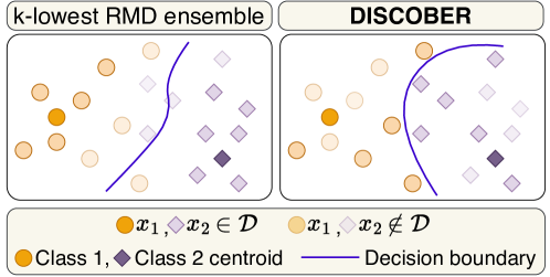
Figure 6: DISCOBER helps in finding a tighter decision boundary due to having a higher probability of including high RMD scored samples in the ensemble of generated data $\mathcal{D}$. Intuitively, high RMD scored samples are farther away from their class prototype but closer to other class samples in comparison to low RMD scored samples which are concentrated closer around the class prototype. Note that DISCOBER includes not only high RMD samples but also some low RMD (i.e., class-representative) samples.

The RMD [30] score of a sample $(x_{i},y_{i})$ is defined as follows:

$$\begin{gathered}\mathcal{RMD}(x_{i},y_{i})=\mathcal{M}_{cls}(x_{i},y_{i})-\mathcal{M}_{\mathrm{agn}}(x_{i}),\\ \mathcal{M}_{cls}(x_{i},y_{i})=-\left(G(x_{i})-\mu_{y_{i}}\right)^{T}\Sigma^{-1}\left(G(x_{i})-\mu_{y_{i}}\right),\\ \mathcal{M}_{\mathrm{agn}}(x_{i})=-\left(G(x_{i})-\mu_{agn}\right)^{T}\Sigma^{-1}_{agn}\left(G(x_{i})-\mu_{agn}\right),\end{gathered}$$ (3)

where $G$ represents the feature extractor, $\mathcal{M}_{cls}(x_{i},y_{i})$ denotes the Mahalanobis distance from $G(x_{i})$ to the corresponding class mean vector $\mu_{y_{i}}=\frac{1}{N_{i}}\sum_{y_{j}=y_{i}}G(x_{j})$, with $N_{i}$ being the count of samples labeled as $y_{i}$, $\Sigma^{-1}$ denotes the inverse of the averaged covariance matrix across classes. Furthermore, $\mathcal{M}_{\mathrm{agn}}(x_{i})$ represents the class-agnostic Mahalanobis distance, where $\mu_{\mathrm{agn}}$ denotes the overall sample mean, and $\Sigma^{-1}_{\mathrm{agn}}$ denotes the inverse covariance for the class-agnostic case.

In the online CL setup, where data arrive in a continuous stream, it is not feasible to calculate $\mu$ and $\Sigma$ of the entire dataset. Instead, a necessity arises to continuously update these statistical parameters to accommodate the dynamic nature of the incoming data stream.

Starting with the initially computed mean vector $\mu_{y_{i}}$ and covariance matrix $\Sigma$ from $N$ samples, the arrival of a new sample $x_{N+1}$ triggers an update. The updated mean vector $\mu_{\text{new}}$ is computed incrementally using a simple moving average (SMA), as follows:

$$\mu_{\text{new}}=\frac{N\mu_{\text{old}}+x_{N+1}}{N+1}.$$ (4)

Similarly, we calculate $\Sigma$ using a simple moving variance. Specifically, the update for the new covariance matrix $\Sigma_{\text{new}}$ is calculated using the deviation of the new sample from the old mean $\Delta=x_{N+1}-\mu_{\text{old}}$, and its deviation from the new mean $\Delta_{\text{new}}=x_{N+1}-\mu_{\text{new}}$.

Formally, we formulate the update process as follows:

$$\Sigma_{\text{new}}=\frac{1}{N+1}\left(N\Sigma_{\text{old}}+\Delta\Delta_{\text{new}}^{T}\right).$$ (5)

The update process for the class-agnostic mean vector $\mu_{\mathrm{agn}}$ and covariance $\Sigma_{\mathrm{agn}}$ follows the same incremental approach as described for the class-specific components.

DISCOBER includes a significant number of samples with high RMD scores in the ensemble dataset. Not only does it include samples with the highest RMD scores, but it also probabilistically incorporates samples with low RMD scores. This approach ensures a core-set ensemble, and we illustrate the effect of DISCOBER in Fig. 6

Appendix 0.E RMD Ablation

We calculate the RMD score for each meta-prompt and summarize the results in Tab. 7. Based on the varied distribution of RMD scores for each meta-prompt, it can be observed that using a diversified set of prompts, rather than a single prompt, allows for the generation of samples ranging from easy to difficult. In other words, it ensures a broader coverage of the sample difficulty spectrum, capturing a more comprehensive representation of the underlying data characteristics.

In addition, we illustrate samples generated from prompts for low RMD samples and high RMD samples in Fig. 7.

Table 7: Average RMD score for meta prompts. For each meta prompt, we generate four prompt rewrites. The average RMD score refers to the average of RMD scores obtained from all images generated using each meta prompt and its corresponding rewritten prompts.

Meta prompt	Average RMD score
A black and white image of [concept] highlighting dramatic contrasts.	-3.471
A minimalist image of [concept] using clean lines and muted colors.	-1.153
A photo of [concept] in analogous colors.	-0.618
A photo of [concept] in complementary colors.	-1.216
A photo of [concept] in earth tones.	1.568
A photo of [concept] in neutral tones.	1.779
This is an image of the [concept].	0.492
A realistic image of [concept].	1.203
A vintage photograph of [concept] with a warm, faded aesthetic.	2.425
A high-resolution photo of [concept] capturing fine details.	-0.446

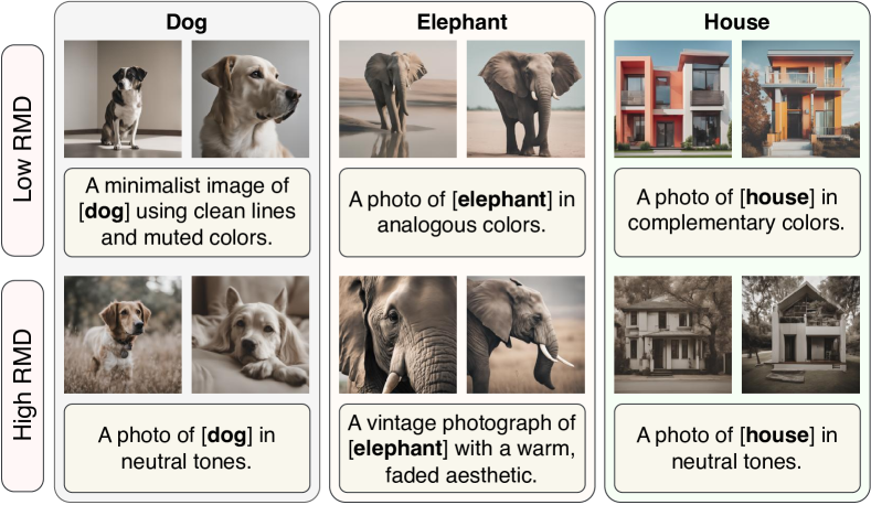
Figure 7: Examples of generated images representing the concepts "Dog," "Elephant," and "House" from the PACS dataset [144]. The images in the top row are generated from meta-prompts with low RMD scores, while the images in the bottom row are generated from meta-prompts with high RMD scores.

Appendix 0.F Scaling behavior

As examining the behavior of in-distribution (ID) accuracy and out-of-distribution (OOD) accuracy with respect to the volume of PACS generated data in Sec. 5.5, we also empirically analyze the scaling behavior in the CCT dataset in Fig. 8. When using both ResNet-18 and ViT as the backbone architecture, the OOD and ID performance increases linearly with the volume of generated data. It shows that with sufficient computational resources to generate more data, it is possible to achieve good performance without any manually annotated data.

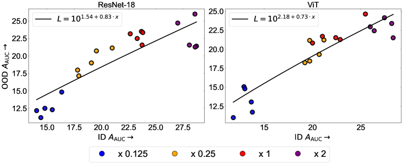
Figure 8: Ensemble scaling behavior of (a) ResNet-18 [47] and (b) ViT [103] for ID $A_{\text{AUC}}$ vs. OOD $A_{\text{AUC}}$ on the CCT dataset [12] using ER [99]. (x 1) denotes the ensemble volume in primary experiments, the default data budget.

Appendix 0.G Experimental Results on CIFAR-10-W using ViT

We compared manually annotated (MA) data and generated data using DISCOBER with Vision Transformer (ViT) [103] as the backbone architecture on CIFAR-10-W [118]. As mentioned in Sec. 5.2, since CIFAR-10-W consists of only two domains, both are used to evaluate the out-of-distribution (OOD) domain. Additionally, since CIFAR-10-W is a web-scraped dataset, the domain of CIFAR-10-W and the web-scraped data are the same. Therefore, we excluded web-scraped data in experiments on CIFAR-10-W and only evaluated OOD performance. We summarize the results in Tab. 8.

Table 8: Comparison of Manually Annotated (MA) data and DISCOBER on CIFAR-10-W. We use ViT as the backbone.

Method	Training Data	$A_{\text{AUC}}\ \uparrow$	$A_{last}\ \uparrow$
ER	DISCOBER	43.70$\pm$0.60	26.55$\pm$1.01
	MA	42.31$\pm$1.15	24.81$\pm$1.20
ER-MIR	DISCOBER	38.30$\pm$0.82	17.79$\pm$1.13
	MA	32.69$\pm$1.39	16.06$\pm$1.73
DER++	DISCOBER	38.31$\pm$0.82	17.80$\pm$1.13
	MA	36.54$\pm$1.15	16.91$\pm$1.02
ASER	DISCOBER	43.67$\pm$0.49	25.83$\pm$1.19
	MA	42.48$\pm$1.14	24.24$\pm$1.23
MEMO	DISCOBER	36.60$\pm$1.09	16.24$\pm$0.65
	MA	34.15$\pm$0.35	14.20$\pm$0.62

Appendix 0.H Details about Web-Scrapping

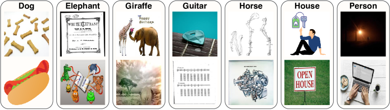
Figure 9: Examples of noisy raw data obtained via web-scraping for the classes in the PACS [144] dataset.

For the collection of our web dataset, we use three search engines: Flickr, Google, and Bing. To ensure a stable collection, we separate the process into querying (collecting URLs) and downloading. Specifically, for Flickr, we use its official API to collect URLs. However, since Google and Bing do not offer official image search APIs, utilize the publicly available querying tool to collect URLs, following [93]. Taking into account the possible errors in the URLs or the download process, we gather URLs corresponding to 1.4 times larger than we need. After collecting the URLs from each search engine, we use a multi-threaded downloader to quickly download the images, following [93].

For Flickr, we are able to download approximately 500 images per minute due to the rapid URL collection facilitated by the official API. Meanwhile, for Google and Bing, the download rate is slower, at approximately 100 images per minute on a single CPU machine. However, the download rate depends on network conditions, as well as the status of the API and the search engine.

Raw images downloaded from search engines might contain uncurated (i.e., noisy) data, as shown in Fig. 9. To address this issue, a previous study [93] addressed the ambiguity of queries through manual query design, such as appending an auxiliary suffix to refine queries. However, in an online CL scenario, where new concepts stream in real-time, such handcrafted query designs for each concept are limited.

In summary, data noise, network dependency, and the need for manual query design specific to each concept restrict the use of web-scrapped data in real-world scenarios where new concepts are encountered in real-time.

Appendix 0.I Prompt Refiner Module $\psi$

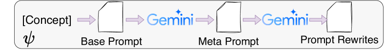
Figure 10: Prompt Refiner Module ($\psi$): Given a [concept], $\psi$ utilizes a pretrained frozen LLM to generate fine-grained prompt-rewrites in a two-step process.

The prompt refiner module ($\psi$) is a crucial component within our proposed G-NoCL framework. With the observed limited diversity in images generated from the same base prompt using a Text-to-Image (T2I) generator, the primary objective of $\psi$ is to facilitate fine-grained prompt rewrites, thereby enhancing the diversity of the generated images. These prompt rewrites aim to cover a broad spectrum of the [concept] by considering various settings, backgrounds, and texture details.

As mentioned in 4.1, a novel concept is conveyed as a stream input to $\psi$. This [concept] is then transformed into the base prompt following the template: "This is an image of the [concept]", a prompt widely used in existing studies [108, 112]. Subsequently, we rewrite 10 different prompts, named meta-prompts, using the base prompt and the Gemini [121] Language Model (LLM). Next, we generate four rewritten prompts per each meta-prompt using the Gemini, resulting in a total set of 50 prompts. These 50 prompts serve as queries for the T2I generators $\mathcal{G}$. It is important to note that our proposed end-to-end framework operates in a zero-shot manner i.e., it does not involve gradient-based training. Furthermore, the prompts, which have been rewritten using the Gemini, are used as-is without any manually selection process.

When designing $\psi$, two key aspects need to be considered: (i) choosing the appropriate Language Model (LLM) and (ii) deciding on the number of stages for prompt rewrite generation.

0.I.1 LLM selection

0.I.1.1 Meta-prompts

We consider two prominent Large Language Models (LLMs) for integration into the $\psi$ module: (i) GPT-3.5 [17], and (ii) Gemini [121]. To select the appropriate LLM, we compare the quality, diversity, and applicability of the meta-prompts generated from the same base prompt using both LLMs.

The meta-prompts generated by GPT-3.5 are as follows:

1. "Generate an image representing [concept]."

2. "This is an image of what? - [concept]"

3. "Show me a visual depiction of [concept]."

4. "Create an artistic representation for [concept]."

5. "Generate an image that encapsulates the essence of [concept]."

6. "Produce a visual interpretation corresponding to [concept]."

7. "Illustrate [concept] in the form of an image."

8. "What does an image portraying [concept] look like?"

9. "Create a visual concept for [concept]."

10. "Generate an artistic rendering reflective of [concept]."

Unlike GPT-3.5, Gemini generates more diversified prompts, since it supports a wide range of background & setting. The meta-prompts generated by Gemini are as follows:

1. Style & Detail:

   1. High-resolution photo: A high-resolution photo of [concept] capturing fine details.

   2. Photorealistic: A realistic image of [concept].

   3. Vintage: A vintage photograph of [concept] with a warm, faded aesthetic.

   4. Black and White: A black and white image of [concept] highlighting dramatic contrasts.

   5. Minimalist: A minimalist image of [concept] using clean lines and muted colors.

2. Color & Pattern:

   1. Analogous colors: A photo of [concept] in analogous colors.

   2. Complementary colors: A photo of [concept] in complementary colors.

   3. Earth tones: A photo of [concept] in earth tones.

   4. Neutral tones: A photo of [concept] in neutral tones.

Table 9: Average cosine similarity of normalized embeddings of the meta-prompts generated via GPT-3.5 [17] and Gemini [121] evaluated using standard sentence embedding models [115, 84, 37, 44]. Lower similarity score indicates higher diversity in the meta-prompts.

LLM	GISTEmbed-L [115]	mxbai-embed-L	Sentence-T5-B [84]	LaBSE [37]	Jina-v2 [44]
GPT-3.5 [17]	0.8552	0.8811	0.944	0.7602	0.9089
Gemini [121]	0.8088	0.8544	0.9137	0.7187	0.8987

We observe that Gemini provides a more diverse set of meta-prompts in comparison to the ones provided by GPT-3.5, which appear to be rather rephrasing of the original base-prompt excluding a few like "Generate an artistic rendering reflective of [concept]." Furthermore, we assess the intra-similarity of the meta-prompts generated by GPT-3.5 and Gemini by calculating the average cosine similarity using normalized embeddings generated by state-of-the-art sentence embedding models, and summarize the results in Table 9. The results show that Gemini consistently achieves a lower average cosine similarity compared to GPT-3.5. In other words, Gemini demonstrates higher diversity in its generated meta-prompts. Therefore, we use the meta-prompts generated by Gemini.

0.I.1.2 Prompt Rewrites

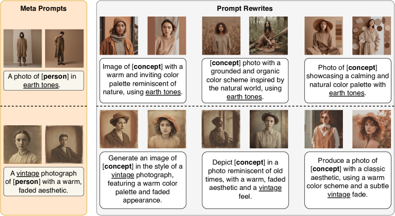
Figure 11: Diversity in generated images using three prompt rewrites of two selected meta prompts for the concept - "person" using SDXL [92].

Based on the 10 meta-prompts provided by the Gemini model (0.I.1.1), we try to rewrite each meta-prompt four distinct ways via Gemini. Effective prompt rewrites play a pivotal role in enhancing diversity among the images generated within the same meta-prompts, as illustrated in Fig. 11. Therefore, the construction of well-crafted prompt rewrites from the predefined meta-prompts is essential.

Note: Along with the 9 meta-prompts, we also use the base-prompt to generate four corresponding prompt rewrites.

The following are the prompt-rewrites provided by Gemini:

1. Original Prompt: A black and white image of [concept] highlighting dramatic contrasts.

   1. High-contrast black and white photo of [concept] emphasizing dramatic lighting.

   2. Black and white [concept] image with bold contrasts, showcasing its form.

   3. Black and white [concept] photography capturing stark shadows and highlights.

   4. Dramatic black and white image of [concept] with deep blacks and bright whites.

2. Original Prompt: A minimalist image of [concept] using clean lines and muted colors.

   1. Simple and elegant photo of [concept] featuring clean lines and muted tones.

   2. Minimalist composition of [concept] with clean lines and a subdued color palette.

   3. Uncluttered image of [concept] using clean lines and muted colors for a serene look.

   4. Photo of [concept] with a minimalist aesthetic, featuring clean lines and soft colors.

3. Original Prompt: A photo of [concept] in analogous colors.

   1. [concept] photo featuring a harmonious blend of analogous colors.

   2. Image of [concept] showcasing a cohesive color scheme using analogous colors.

   3. Photo of [concept] where the colors naturally complement each other, following an analogous color scheme.

   4. [concept] image with a pleasing color palette using analogous colors that sit next to each other on the color wheel.

4. Original Prompt: A photo of [concept] in complementary colors.

   1. Image of [concept] featuring contrasting yet balanced colors, using a complementary color scheme.

   2. Photo of [concept] where the colors create a sense of visual tension through complementary colors.

   3. [concept] image with a vibrant color palette using complementary colors that sit opposite each other on the color wheel.

   4. Photo of [concept] showcasing a dynamic color combination with complementary hues.

5. Original Prompt: A photo of [concept] in earth tones.

   1. Photo of [concept] featuring natural, earthy colors like brown, green, and beige.

   2. Image of [concept] with a warm and inviting color palette reminiscent of nature, using earth tones.

   3. [concept] photo with a grounded and organic color scheme inspired by the natural world, using earth tones.

   4. Photo of [concept] showcasing a calming and natural color palette with earth tones.

6. Original Prompt: A photo of [concept] in neutral tones.

   1. Photo of [concept] featuring a subtle and timeless color palette with neutral tones.

   2. Image of [concept] with a classic and versatile color scheme using neutral tones.

   3. [concept] photo with a sophisticated and understated color palette dominated by neutral tones.

   4. Photo of [concept] where the focus falls on the subject itself through the use of neutral tones.

7. Original Prompt (Base): This is an image of the [concept]

   1. Capture a stunning image of [concept].

   2. Showcase the beauty of [concept] in a photo.

   3. Create a photo that portrays [concept] accurately.

   4. Generate a visually appealing image of [concept].

8. Original Prompt: A realistic image of [concept].

   1. Create a lifelike image of [concept] that captures its true essence.

   2. Generate a photo of [concept] that appears true to life.

   3. Produce an image of [concept] with realistic details and lighting.

   4. Depict [concept] in a photo with a high degree of visual realism.

9. Original Prompt: A vintage photograph of [concept] with a warm, faded aesthetic.

   1. Create a nostalgic photo of [concept] with a warm, vintage tone and faded colors.

   2. Generate an image of [concept] in the style of a vintage photograph, featuring a warm color palette and faded appearance.

   3. Produce a photo of [concept] with a classic aesthetic, using a warm color scheme and a subtle vintage fade.

   4. Depict [concept] in a photo reminiscent of old times, with a warm, faded aesthetic and a vintage feel.

10. Original Prompt: A high-resolution photo of [concept] capturing fine details.

    1. Close-up photo of [concept] in high resolution, revealing intricate details.

    2. Detailed, high-resolution image of [concept] showcasing its intricate features.

    3. Sharp, high-resolution photo of [concept] capturing every minute detail.

    4. Crystal clear photo of [concept] in high resolution, showing fine textures and patterns.

0.I.2 Number of Prompt Rewrite Stages

In an effort to illustrate the rationale behind the two-step process, creating meta-prompts and then rewriting each meta-prompt into multiple prompts, in $\psi$, we explore the single-step generation, which directly generates a complete set of prompt rewrites from the base prompt using the Gemini model.

The prompts generated through single-step generation are as follows:

1. Direct phrasing:

   1. Depict [concept].

   2. Generate an image of [concept].

   3. Show me a picture of [concept].

   4. Create a visual representation of [concept].

   5. Display an image containing [concept].

2. Descriptive phrasing:

   1. A photorealistic image of a [concept].

   2. A detailed illustration of a [concept].

   3. A high-resolution picture of a [concept] in its natural habitat.

   4. A close-up image of a [concept], showcasing its intricate details.

   5. A vibrant painting depicting a [concept] in action.

3. Action-oriented phrasing:

   1. Capture the essence of a [concept] in an image.

   2. Bring a [concept] to life with a stunning image.

   3. Showcase the beauty of a [concept] in a captivating image.

   4. Visualize a [concept] using your creative vision.

   5. Generate an image that embodies the concept of [concept].

4. Context-specific phrasing:

   1. Imagine a [concept] exploring a bustling city.

   2. Depict a [concept] resting peacefully in a serene landscape.

   3. Capture the playful energy of a [concept] in an image.

   4. Generate an image of a [concept] interacting with its environment.

   5. Showcase the unique characteristics of a [concept] in detail.

5. Emotional phrasing:

   1. Generate an image that evokes the majesty of a [concept].

   2. Capture the tranquility of a [concept] in its natural habitat.

   3. Showcase the playful joy of a [concept] in motion.

   4. Depict the power and strength of a [concept] visually.

   5. Generate an image that captures the essence of a [concept]’s beauty.

6. Figurative language:

   1. Paint a picture of a [concept] coming to life.

   2. Sculpt a visual representation of a [concept].

   3. Weave a tapestry depicting the image of a [concept].

   4. Compose a portrait of a [concept] in its element.

   5. Capture the essence of a [concept] through the lens of imagination.

7. Storytelling:

   1. Tell the story of a [concept] through a captivating image.

   2. Unfold a narrative around a [concept] through visual storytelling.

   3. Generate an image that sparks a story about a [concept].

   4. Capture a moment in the life of a [concept] with a stunning image.

   5. Showcase the journey of a [concept] through a series of images.

8. Additional variations:

   1. A photo of [concept] in its natural environment.

   2. A vintage postcard depicting [concept].

   3. A pixel art rendition of [concept].

   4. A sketch capturing the essence of [concept].

   5. A classic painting style interpretation of [concept].

   6. A hyper-realistic image of [concept].

   7. A watercolor painting capturing the serenity of a [concept].

   8. A futuristic illustration of a [concept].

   9. A surreal depiction of a [concept] in a dreamlike setting.

   10. An animated GIF showcasing the movement of a [concept].

   11. A close-up portrait of a [concept] with its unique features highlighted.

   12. A panoramic view showcasing the vastness of a [concept]’s habitat.

   13. A minimalist interpretation of [concept] using simple lines and shapes.

   14. An abstract representation of the essence of [concept] using color and form.

   15. A photo of a [concept] interacting with humans (if applicable).

Although several prompts, rewritten using the base prompt, exhibit qualitative merit, a considerable number of them lack universal applicability across diverse concepts. For instance, prompts generated under context-specific phrasing, such as "Imagine a [concept] exploring a bustling city", generate only images related to a particular domain, which could potentially harm domain generalization performance.

In the future, as LLMs advance and better approaches for prompt diversification are proposed, we expect more diversified images to be generated, increasing the utility of G-NoCL.

References

- [1] Agun, H.V.: Webcollectives: A light regular expression based web content extractor in java. In: SoftwareX. vol. 24, p. 101569. Elsevier (2023)
- [2] Aljundi, R., Babiloni, F., Elhoseiny, M., Rohrbach, M., Tuytelaars, T.: Memory aware synapses: Learning what (not) to forget. In: ECCV (2018)
- [3] Aljundi, R., Caccia, L., Belilovsky, E., Caccia, M., Lin, M., Charlin, L., Tuytelaars, T.: Online continual learning with maximally interfered retrieval. In: NeurIPS (2019)
- [4] Aljundi, R., Lin, M., Goujaud, B., Bengio, Y.: Gradient based sample selection for online continual learning. In: NeurIPS (2019)
- [5] Anonymous: Coreset selection for object detection (2023), https://openreview.net/forum?id=Yyg3DXzaIK
- [6] Attia, J.: Evaluating the effectiveness of common technical trading models. arXiv preprint arXiv:1907.10407 (2019)
- [7] Azizi, S., Kornblith, S., Saharia, C., Norouzi, M., Fleet, D.J.: Synthetic data from diffusion models improves imagenet classification. arXiv preprint arXiv:2304.08466 (2023)
- [8] Bain, M., Nagrani, A., Varol, G., Zisserman, A.: Frozen in time: A joint video and image encoder for end-to-end retrieval. In: ICCV (2021)
- [9] Balloccu, S., Schmidtová, P., Lango, M., Dušek, O.: Leak, cheat, repeat: Data contamination and evaluation malpractices in closed-source llms. arXiv preprint arXiv:2402.03927 (2024)
- [10] Banerjee, S., Verma, V.K., Mukherjee, A., Gupta, D., Namboodiri, V.P., Rai, P.: Verse: Virtual-gradient aware streaming lifelong learning with anytime inference. arXiv preprint arXiv:2309.08227 (2023)
- [11] Bang, J., Kim, H., Yoo, Y., Ha, J.W., Choi, J.: Rainbow memory: Continual learning with a memory of diverse samples. In: CVPR (2021)
- [12] Beery, S., Van Horn, G., Perona, P.: Recognition in terra incognita. In: ECCV (2018)
- [13] Betker, J., Goh, G., Jing, L., Brooks, T., Wang, J., Li, L., Ouyang, L., Zhuang, J., Lee, J., Guo, Y., et al.: Improving image generation with better captions. Computer Science. https://cdn.openai.com/papers/dall-e-3.pdf 2(3), 8 (2023)
- [14] Bianchi, F., Kalluri, P., Durmus, E., Ladhak, F., Cheng, M., Nozza, D., Hashimoto, T., Jurafsky, D., Zou, J., Caliskan, A.: Easily accessible text-to-image generation amplifies demographic stereotypes at large scale. In: FAccT (2023)
- [15] Bonicelli, L., Boschini, M., Porrello, A., Spampinato, C., Calderara, S.: On the effectiveness of lipschitz-driven rehearsal in continual learning. In: NeurIPS (2022)
- [16] Boschini, M., Bonicelli, L., Buzzega, P., Porrello, A., Calderara, S.: Class-incremental continual learning into the extended der-verse. In: TPAMI. IEEE (2022)
- [17] Brown, T., Mann, B., Ryder, N., Subbiah, M., Kaplan, J.D., Dhariwal, P., Neelakantan, A., Shyam, P., Sastry, G., Askell, A., et al.: Language models are few-shot learners. In: NeurIPS (2020)
- [18] Buzzega, P., Boschini, M., Porrello, A., Abati, D., Calderara, S.: Dark experience for general continual learning: a strong, simple baseline. In: NeurIPS (2020)
- [19] Byeon, M., Park, B., Kim, H., Lee, S., Baek, W., Kim, S.: Coyo-700m: Image-text pair dataset. https://github.com/kakaobrain/coyo-dataset (2022)
- [20] Caccia, L., Xu, J., Ott, M., Ranzato, M., Denoyer, L.: On anytime learning at macroscale. In: CoLLAs. PMLR (2022)
- [21] Cai, R., Cui, Y., Li, Z., Yu, Z., Li, H., Hu, Y., Kot, A.: Rehearsal-free domain continual face anti-spoofing: Generalize more and forget less. arXiv preprint arXiv:2303.09914 (2023)
- [22] Caliskan, A., Bryson, J.J., Narayanan, A.: Semantics derived automatically from language corpora contain human-like biases. Science 356(6334), 183–186 (2017)
- [23] Carlini, N., Jagielski, M., Choquette-Choo, C.A., Paleka, D., Pearce, W., Anderson, H., Terzis, A., Thomas, K., Tramèr, F.: Poisoning web-scale training datasets is practical. arXiv preprint arXiv:2302.10149 (2023)
- [24] Carvalho, T., Moniz, N., Antunes, L., Chawla, N.: Differentially-private data synthetisation for efficient re-identification risk control. arXiv preprint arXiv:2212.00484 (2022)
- [25] Chang, A., Fontaine, M.C., Booth, S., Matarić, M.J., Nikolaidis, S.: Quality-diversity generative sampling for learning with synthetic data. arXiv preprint arXiv:2312.14369 (2023)
- [26] Chen, Q., Xiang, C., Xue, M., Li, B., Borisov, N., Kaarfar, D., Zhu, H.: Differentially private data generative models. arXiv preprint arXiv:1812.02274 (2018)
- [27] Chen, X., Navidi, T., Ermon, S., Rajagopal, R.: Distributed generation of privacy preserving data with user customization. arXiv preprint arXiv:1904.09415 (2019)
- [28] Cheung, B., Terekhov, A., Chen, Y., Agrawal, P., Olshausen, B.: Superposition of many models into one. In: NeurIPS (2019)
- [29] Cubuk, E.D., Zoph, B., Shlens, J., Le, Q.V.: Randaugment: Practical automated data augmentation with a reduced search space. In: CVPRW (2020)
- [30] Cui, P., Zhang, D., Deng, Z., Dong, Y., Zhu, J.: Learning sample difficulty from pre-trained models for reliable prediction. In: NeurIPS (2024)
- [31] Dekoninck, J., Müller, M.N., Baader, M., Fischer, M., Vechev, M.: Evading data contamination detection for language models is (too) easy. arXiv preprint arXiv:2402.02823 (2024)
- [32] Deng, J., Dong, W., Socher, R., Li, L.J., Li, K., Fei-Fei, L.: Imagenet: A large-scale hierarchical image database. In: CVPR (2009). https://doi.org/10.1109/CVPR.2009.5206848
- [33] Ding, M., Zheng, W., Hong, W., Tang, J.: Cogview2: Faster and better text-to-image generation via hierarchical transformers. In: NeurIPS (2022)
- [34] Dosovitskiy, A., Brox, T.: Inverting visual representations with convolutional networks. In: CVPR (2016)
- [35] Fan, L., Chen, K., Krishnan, D., Katabi, D., Isola, P., Tian, Y.: Scaling laws of synthetic images for model training… for now. arXiv preprint arXiv:2312.04567 (2023)
- [36] Fan, L., Krishnan, D., Isola, P., Katabi, D., Tian, Y.: Improving clip training with language rewrites. In: NeurIPS (2024)
- [37] Feng, F., Yang, Y., Cer, D., Arivazhagan, N., Wang, W.: Language-agnostic BERT sentence embedding. In: Muresan, S., Nakov, P., Villavicencio, A. (eds.) Proceedings of the 60th Annual Meeting of the Association for Computational Linguistics (Volume 1: Long Papers). pp. 878–891. Association for Computational Linguistics, Dublin, Ireland (May 2022). https://doi.org/10.18653/v1/2022.acl-long.62, https://aclanthology.org/2022.acl-long.62
- [38] Foerderer, J.: Should we trust web-scraped data? arXiv preprint arXiv:2308.02231 (2023)
- [39] Fraser, K.C., Kiritchenko, S., Nejadgholi, I.: Diversity is not a one-way street: Pilot study on ethical interventions for racial bias in text-to-image systems. In: ICCV (2023)
- [40] Gao, L., Biderman, S., Black, S., Golding, L., Hoppe, T., Foster, C., Phang, J., He, H., Thite, A., Nabeshima, N., et al.: The pile: An 800gb dataset of diverse text for language modeling. arXiv preprint arXiv:2101.00027 (2020)
- [41] Ghunaim, Y., Bibi, A., Alhamoud, K., Alfarra, M., Al Kader Hammoud, H.A., Prabhu, A., Torr, P.H., Ghanem, B.: Real-time evaluation in online continual learning: A new hope. In: CVPR (2023)
- [42] Gu, J., Gao, Q., Zhai, S., Chen, B., Liu, L., Susskind, J.: Learning controllable 3d diffusion models from single-view images. arXiv preprint arXiv:2304.06700 (2023)
- [43] Guo, C., Benitez-Quiroz, F., Feng, Q., Martinez, A.: Structural similarity: When to use deep generative models on imbalanced image dataset augmentation. arXiv preprint arXiv:2303.04854 (2023)
- [44] Günther, M., Ong, J., Mohr, I., Abdessalem, A., Abel, T., Akram, M.K., Guzman, S., Mastrapas, G., Sturua, S., Wang, B., Werk, M., Wang, N., Xiao, H.: Jina embeddings 2: 8192-token general-purpose text embeddings for long documents (2023)
- [45] Harun, M.Y., Gallardo, J., Kanan, C.: Grasp: A rehearsal policy for efficient online continual learning. arXiv preprint arXiv:2308.13646 (2023)
- [46] Hayes, T.L., Kafle, K., Shrestha, R., Acharya, M., Kanan, C.: Remind your neural network to prevent catastrophic forgetting. In: ECCV (2020)
- [47] He, K., Zhang, X., Ren, S., Sun, J.: Deep residual learning for image recognition. In: CVPR (2016)
- [48] Henderson, P., Li, X., Jurafsky, D., Hashimoto, T., Lemley, M.A., Liang, P.: Foundation models and fair use. arXiv preprint arXiv:2303.15715 (2023)
- [49] Hernandez, D., Kaplan, J., Henighan, T., McCandlish, S.: Scaling laws for transfer. arXiv preprint arXiv:2102.01293 (2021)
- [50] Hoffmann, J., Borgeaud, S., Mensch, A., Buchatskaya, E., Cai, T., Rutherford, E., Casas, D.d.L., Hendricks, L.A., Welbl, J., Clark, A., et al.: Training compute-optimal large language models. arXiv preprint arXiv:2203.15556 (2022)
- [51] Huang, Q., Park, D.S., Wang, T., Denk, T.I., Ly, A., Chen, N., Zhang, Z., Zhang, Z., Yu, J., Frank, C., et al.: Noise2music: Text-conditioned music generation with diffusion models. arXiv preprint arXiv:2302.03917 (2023)
- [52] Huang, R., Huang, J., Yang, D., Ren, Y., Liu, L., Li, M., Ye, Z., Liu, J., Yin, X., Zhao, Z.: Make-an-audio: Text-to-audio generation with prompt-enhanced diffusion models. arXiv preprint arXiv:2301.12661 (2023)
- [53] Jadon, A., Kumar, S.: Leveraging generative ai models for synthetic data generation in healthcare: Balancing research and privacy. arXiv preprint arXiv:2305.05247 (2023)
- [54] Jain, A., Memon, N., Togelius, J.: Fair gans through model rebalancing with synthetic data. arXiv preprint arXiv:2308.08638 (2023)
- [55] Kang, M., Min, D., Hwang, S.J.: Any-speaker adaptive text-to-speech synthesis with diffusion models. arXiv preprint arXiv:2211.09383 (2022)
- [56] Karnewar, A., Vedaldi, A., Novotny, D., Mitra, N.J.: Holodiffusion: Training a 3d diffusion model using 2d images. In: CVPR (2023)
- [57] Katirai, A., Garcia, N., Ide, K., Nakashima, Y., Kishimoto, A.: Situating the social issues of image generation models in the model life cycle: a sociotechnical approach. arXiv preprint arXiv:2311.18345 (2023)
- [58] Khader, F., Mueller-Franzes, G., Arasteh, S.T., Han, T., Haarburger, C., Schulze-Hagen, M., Schad, P., Engelhardt, S., Baessler, B., Foersch, S., et al.: Medical diffusion–denoising diffusion probabilistic models for 3d medical image generation. arXiv preprint arXiv:2211.03364 (2022)
- [59] Khan, M., Hanna, A.: The legality of computer vision datasets. Under review (2020)
- [60] Kim, B., Seo, M., Choi, J.: Online continual learning for interactive instruction following agents. In: OpenReview (2024), https://openreview.net/forum?id=7M0EzjugaN
- [61] Kiran, M., Pedersoli, M., Dolz, J., Blais-Morin, L.A., Granger, E., et al.: Incremental multi-target domain adaptation for object detection with efficient domain transfer. In: PR (2022)
- [62] Kirkpatrick, J., Pascanu, R., Rabinowitz, N., Veness, J., Desjardins, G., Rusu, A.A., Milan, K., Quan, J., Ramalho, T., Grabska-Barwinska, A., et al.: Overcoming catastrophic forgetting in neural networks. In: PNAS (2017)
- [63] Kocetkov, D., Li, R., Allal, L.B., Li, J., Mou, C., Ferrandis, C.M., Jernite, Y., Mitchell, M., Hughes, S., Wolf, T., et al.: The stack: 3 tb of permissively licensed source code. arXiv preprint arXiv:2211.15533 (2022)
- [64] Koh, H., Kim, D., Ha, J.W., Choi, J.: Online continual learning on class incremental blurry task configuration with anytime inference. In: ICLR (2021)
- [65] Koh, H., Seo, M., Bang, J., Song, H., Hong, D., Park, S., Ha, J.W., Choi, J.: Online boundary-free continual learning by scheduled data prior. In: ICLR (2023)
- [66] Krizhevsky, A., Hinton, G., et al.: Learning multiple layers of features from tiny images (2009)
- [67] Kumar, V., Choudhary, A., Cho, E.: Data augmentation using pre-trained transformer models. arXiv preprint arXiv:2003.02245 (2020)
- [68] Lee, K., Lee, K., Lee, H., Shin, J.: A simple unified framework for detecting out-of-distribution samples and adversarial attacks. In: NeurIPS (2018)
- [69] Lesort, T., Stoian, A., Filliat, D.: Regularization shortcomings for continual learning. arXiv preprint arXiv:1912.03049 (2019)
- [70] Li, W., Wang, L., Li, W., Agustsson, E., Van Gool, L.: Webvision database: Visual learning and understanding from web data. arXiv preprint arXiv:1708.02862 (2017)
- [71] Li, X., Zhou, Y., Wu, T., Socher, R., Xiong, C.: Learn to grow: A continual structure learning framework for overcoming catastrophic forgetting. In: ICML. PMLR (2019)
- [72] Li, Y.: An open source data contamination report for llama series models. arXiv preprint arXiv:2310.17589 (2023)
- [73] Liang, J., Wu, C., Hu, X., Gan, Z., Wang, J., Wang, L., Liu, Z., Fang, Y., Duan, N.: Nuwa-infinity: Autoregressive over autoregressive generation for infinite visual synthesis. In: NeurIPS (2022)
- [74] Liu, C., Wang, L., Lyu, L., Sun, C., Wang, X., Zhu, Q.: Deja vu: Continual model generalization for unseen domains. In: ICLR (2022)
- [75] Liu, G., Li, Y., Fei, Z., Fu, H., Luo, X., Guo, Y.: Prefix-diffusion: A lightweight diffusion model for diverse image captioning. arXiv preprint arXiv:2309.04965 (2023)
- [76] Lukas, N., Salem, A., Sim, R., Tople, S., Wutschitz, L., Zanella-Béguelin, S.: Analyzing leakage of personally identifiable information in language models. arXiv preprint arXiv:2302.00539 (2023)
- [77] Madaan, D., Yoon, J., Li, Y., Liu, Y., Hwang, S.J.: Representational continuity for unsupervised continual learning. arXiv preprint arXiv:2110.06976 (2021)
- [78] Meng, Y., Huang, J., Zhang, Y., Han, J.: Generating training data with language models: Towards zero-shot language understanding. In: NeurIPS (2022)
- [79] Mimura, M., Ueno, S., Inaguma, H., Sakai, S., Kawahara, T.: Leveraging sequence-to-sequence speech synthesis for enhancing acoustic-to-word speech recognition. In: SLT. IEEE (2018)
- [80] Mirza, M.J., Masana, M., Possegger, H., Bischof, H.: An efficient domain-incremental learning approach to drive in all weather conditions. In: CVPR (2022)
- [81] Misra, D., Runwal, B., Chen, T., Wang, Z., Rish, I.: App: Anytime progressive pruning. arXiv preprint arXiv:2204.01640 (2022)
- [82] Murgia, M., Harlow, M.: Who’s using your face? the ugly truth about facial recognition. Financial Times 19, 1 (2019)
- [83] Neyshabur, B., Sedghi, H., Zhang, C.: What is being transferred in transfer learning? In: NeurIPS (2020)
- [84] Ni, J., Abrego, G.H., Constant, N., Ma, J., Hall, K.B., Cer, D., Yang, Y.: Sentence-t5: Scalable sentence encoders from pre-trained text-to-text models. arXiv preprint arXiv:2108.08877 (2021)
- [85] Nie, W., Vahdat, A., Anandkumar, A.: Controllable and compositional generation with latent-space energy-based models. In: NeurIPS (2021)
- [86] Niu, L., Tang, Q., Veeraraghavan, A., Sabharwal, A.: Learning from noisy web data with category-level supervision. In: CVPR (2018)
- [87] O’Sullivan, L.: Don’t steal data. In: NeurIPSW (2020)
- [88] Packer, B., Mitchell, M., Guajardo-Céspedes, M., Halpern, Y.: Text embeddings contain bias. here’s why that matters. (2018)
- [89] Panagiotakopoulos, T., Dovesi, P.L., Härenstam-Nielsen, L., Poggi, M.: Online domain adaptation for semantic segmentation in ever-changing conditions. In: ECCV (2022)
- [90] Parisi, G.I., Kemker, R., Part, J.L., Kanan, C., Wermter, S.: Continual lifelong learning with neural networks: A review. In: Neural networks (2019)
- [91] Pellegrini, L., Graffieti, G., Lomonaco, V., Maltoni, D.: Latent replay for real-time continual learning. In: IROS. IEEE (2020)
- [92] Podell, D., English, Z., Lacey, K., Blattmann, A., Dockhorn, T., Müller, J., Penna, J., Rombach, R.: Sdxl: Improving latent diffusion models for high-resolution image synthesis. arXiv preprint arXiv:2307.01952 (2023)
- [93] Prabhu, A., Hammoud, H.A.A.K., Lim, S.N., Ghanem, B., Torr, P.H., Bibi, A.: From categories to classifier: Name-only continual learning by exploring the web. arXiv preprint arXiv:2311.11293 (2023)
- [94] Qi, D., Zhao, H., Li, S.: Better generative replay for continual federated learning. In: ICLR (2023)
- [95] Quang, J.: Does training ai violate copyright law? Berkeley Tech. LJ 36, 1407 (2021)
- [96] Radford, A., Kim, J.W., Hallacy, C., Ramesh, A., Goh, G., Agarwal, S., Sastry, G., Askell, A., Mishkin, P., Clark, J., et al.: Learning transferable visual models from natural language supervision. In: ICML. PMLR (2021)
- [97] Ramasesh, V.V., Lewkowycz, A., Dyer, E.: Effect of scale on catastrophic forgetting in neural networks. In: ICLR (2022), https://openreview.net/forum?id=GhVS8_yPeEa
- [98] Razzhigaev, A., Shakhmatov, A., Maltseva, A., Arkhipkin, V., Pavlov, I., Ryabov, I., Kuts, A., Panchenko, A., Kuznetsov, A., Dimitrov, D.: Kandinsky: an improved text-to-image synthesis with image prior and latent diffusion. arXiv preprint arXiv:2310.03502 (2023)
- [99] Rolnick, D., Ahuja, A., Schwarz, J., Lillicrap, T., Wayne, G.: Experience replay for continual learning. In: NeurIPS (2019)
- [100] Rombach, R., Blattmann, A., Lorenz, D., Esser, P., Ommer, B.: High-resolution image synthesis with latent diffusion models. In: CVPR (2022)
- [101] Rosenfeld, A., Tsotsos, J.K.: Incremental learning through deep adaptation. In: TPAMI (2018)
- [102] Russakovsky, O., Deng, J., Su, H., Krause, J., Satheesh, S., Ma, S., Huang, Z., Karpathy, A., Khosla, A., Bernstein, M., et al.: Imagenet large scale visual recognition challenge. In: IJCV (2015)
- [103] Rusu, A.A., Rabinowitz, N.C., Desjardins, G., Soyer, H., Kirkpatrick, J., Kavukcuoglu, K., Pascanu, R., Hadsell, R.: Progressive neural networks. arXiv preprint arXiv:1606.04671 (2016)
- [104] Sadat, S., Buhmann, J., Bradely, D., Hilliges, O., Weber, R.M.: Cads: Unleashing the diversity of diffusion models through condition-annealed sampling. arXiv preprint arXiv:2310.17347 (2023)
- [105] Sato, R.: Active learning from the web. In: WWW (2023)
- [106] Schuhmann, C., Beaumont, R., Vencu, R., Gordon, C., Wightman, R., Cherti, M., Coombes, T., Katta, A., Mullis, C., Wortsman, M., et al.: Laion-5b: An open large-scale dataset for training next generation image-text models (2022)
- [107] Seo, M., Koh, H., Choi, J.: Budgeted online continual learning by adaptive layer freezing and frequency-based sampling. In: OpenReview (2024), https://openreview.net/forum?id=3klVRLhK7w
- [108] Shi, Y., Peng, D., Liao, W., Lin, Z., Chen, X., Liu, C., Zhang, Y., Jin, L.: Exploring ocr capabilities of gpt-4v (ision): A quantitative and in-depth evaluation. arXiv preprint arXiv:2310.16809 (2023)
- [109] Shim, D., Mai, Z., Jeong, J., Sanner, S., Kim, H., Jang, J.: Online class-incremental continual learning with adversarial shapley value. In: AAAI (2021)
- [110] Shin, H., Lee, J.K., Kim, J., Kim, J.: Continual learning with deep generative replay. In: NeurIPS (2017)
- [111] Shin, J., Kang, M., Park, J.: Fill-up: Balancing long-tailed data with generative models. arXiv preprint arXiv:2306.07200 (2023)
- [112] Shtedritski, A., Rupprecht, C., Vedaldi, A.: What does clip know about a red circle? visual prompt engineering for vlms. arXiv preprint arXiv:2304.06712 (2023)
- [113] Simon, C., Faraki, M., Tsai, Y.H., Yu, X., Schulter, S., Suh, Y., Harandi, M., Chandraker, M.: On generalizing beyond domains in cross-domain continual learning. In: CVPR (2022)
- [114] Smith, J.S., Tian, J., Halbe, S., Hsu, Y.C., Kira, Z.: A closer look at rehearsal-free continual learning. In: CVPR (2023)
- [115] Solatorio, A.V.: Gistembed: Guided in-sample selection of training negatives for text embedding fine-tuning. arXiv preprint arXiv:2402.16829 (2024), https://arxiv.org/abs/2402.16829
- [116] Solon, O.: Facial recognition’s ‘dirty little secret’: Millions of online photos scraped without consent. In: NBC News. vol. 12 (2019)
- [117] Subramani, N., Luccioni, S., Dodge, J., Mitchell, M.: Detecting personal information in training corpora: an analysis. In: TrustNLP (2023)
- [118] Sun, X., Leng, X., Wang, Z., Yang, Y., Huang, Z., Zheng, L.: Cifar-10-warehouse: Broad and more realistic testbeds in model generalization analysis. In: ICLR (2024)
- [119] Sun, X., Zheng, L., Lai, Y.K., Yang, J.: Learning from web data: the benefit of unsupervised object localization. arXiv preprint arXiv:1812.09232 (2018)
- [120] Tang, J., Nie, Y., Markhasin, L., Dai, A., Thies, J., Nießner, M.: Diffuscene: Scene graph denoising diffusion probabilistic model for generative indoor scene synthesis. arXiv preprint arXiv:2303.14207 (2023)
- [121] Team, G., Anil, R., Borgeaud, S., Wu, Y., Alayrac, J.B., Yu, J., Soricut, R., Schalkwyk, J., Dai, A.M., Hauth, A., et al.: Gemini: a family of highly capable multimodal models. arXiv preprint arXiv:2312.11805 (2023)
- [122] Thiel, D.: Identifying and eliminating csam in generative ml training data and models. Tech. rep., Technical report, Stanford University, Palo Alto, CA, 2023 (2023)
- [123] Tian, Y., Fan, L., Chen, K., Katabi, D., Krishnan, D., Isola, P.: Learning vision from models rivals learning vision from data. arXiv preprint arXiv:2312.17742 (2023)
- [124] Tian, Y., Fan, L., Isola, P., Chang, H., Krishnan, D.: Stablerep: Synthetic images from text-to-image models make strong visual representation learners. In: NeurIPS (2024)
- [125] Tiwari, R., Killamsetty, K., Iyer, R., Shenoy, P.: Gcr: Gradient coreset based replay buffer selection for continual learning. In: CVPR (2022)
- [126] Verwimp, E., Yang, K., Parisot, S., Hong, L., McDonagh, S., Pérez-Pellitero, E., De Lange, M., Tuytelaars, T.: Clad: A realistic continual learning benchmark for autonomous driving. Neural Networks (2023)
- [127] Wang, J., Lan, C., Liu, C., Ouyang, Y., Qin, T., Lu, W., Chen, Y., Zeng, W., Yu, P.: Generalizing to unseen domains: A survey on domain generalization. IEEE Transactions on Knowledge and Data Engineering (2022)
- [128] Wang, Q., Fink, O., Van Gool, L., Dai, D.: Continual test-time domain adaptation. In: CVPR (2022)
- [129] Wang, R., Schmedding, S., Huber, M.F.: Improving the effectiveness of deep generative data. In: WACV (2024)
- [130] Wang, Z., Zhang, Z., Lee, C.Y., Zhang, H., Sun, R., Ren, X., Su, G., Perot, V., Dy, J., Pfister, T.: Learning to prompt for continual learning. In: CVPR (2022)
- [131] Wenger, E., Li, X., Zhao, B.Y., Shmatikov, V.: Data isotopes for data provenance in dnns. arXiv preprint arXiv:2208.13893 (2022)
- [132] Wolfe, R., Yang, Y., Howe, B., Caliskan, A.: Contrastive language-vision ai models pretrained on web-scraped multimodal data exhibit sexual objectification bias. FAccT (2023)
- [133] Xu, W., Zhao, J., Iannacci, F., Wang, B.: Ffpdg: Fast, fair and private data generation. arXiv preprint arXiv:2307.00161 (2023)
- [134] Xu, Z., Liu, Z., Yan, Y., Liu, Z., Xiong, C., Yu, G.: Cleaner pretraining corpus curation with neural web scraping. arXiv preprint arXiv:2402.14652 (2024)
- [135] Xue, L., Constant, N., Roberts, A., Kale, M., Al-Rfou, R., Siddhant, A., Barua, A., Raffel, C.: mt5: A massively multilingual pre-trained text-to-text transformer. arXiv preprint arXiv:2010.11934 (2020)
- [136] Yoon, J., Madaan, D., Yang, E., Hwang, S.J.: Online coreset selection for rehearsal-based continual learning. In: ICLR (2021)
- [137] Yoon, J., Yang, E., Lee, J., Hwang, S.J.: Lifelong learning with dynamically expandable networks. In: ICLR (2018)
- [138] Yuan, Y., Shi, C., Wang, R., Chen, L., Jiang, F., You, Y., Lam, W.: Mcqueen: a benchmark for multimodal conversational query rewrite. In: EMNLP (2022)
- [139] Zenke, F., Poole, B., Ganguli, S.: Continual learning through synaptic intelligence. In: ICML. PMLR (2017)
- [140] Zhang, D., Xia, B., Liu, Y., Xu, X., Hoang, T., Xing, Z., Staples, M., Lu, Q., Zhu, L.: Tag your fish in the broken net: A responsible web framework for protecting online privacy and copyright. arXiv preprint arXiv:2310.07915 (2023)
- [141] Zhang, Y., Zhou, D., Hooi, B., Wang, K., Feng, J.: Expanding small-scale datasets with guided imagination. In: NeurIPS (2024)
- [142] Zhao, Y., Xu, Y., Xiao, Z., Hou, T.: Mobilediffusion: Subsecond text-to-image generation on mobile devices. arXiv preprint arXiv:2311.16567 (2023)
- [143] Zhou, D.W., Wang, Q.W., Ye, H.J., Zhan, D.C.: A model or 603 exemplars: Towards memory-efficient class-incremental learning. In: ICLR (2022)
- [144] Zhou, K., Yang, Y., Hospedales, T., Xiang, T.: Deep domain-adversarial image generation for domain generalisation. In: AAAI (2020)
- [145] Zhou, Z., Yeung, G., Schapiro, A.C.: Self-recovery of memory via generative replay. arXiv preprint arXiv:2301.06030 (2023)
- [146] Zhu, W., Hessel, J., Awadalla, A., Gadre, S.Y., Dodge, J., Fang, A., Yu, Y., Schmidt, L., Wang, W.Y., Choi, Y.: Multimodal c4: An open, billion-scale corpus of images interleaved with text. In: NeurIPS (2024)