Variance-Dependent Regret Bounds for Non-stationary Linear Bandits

Abstract

We investigate the non-stationary stochastic linear bandit problem where the reward distribution evolves each round. Existing algorithms characterize the non-stationarity by the total variation budget $B_{K}$, which is the summation of the change of the consecutive feature vectors of the linear bandits over $K$ rounds. However, such a quantity only measures the non-stationarity with respect to the expectation of the reward distribution, which makes existing algorithms sub-optimal under the general non-stationary distribution setting. In this work, we propose algorithms that utilize the variance of the reward distribution as well as the $B_{K}$, and show that they can achieve tighter regret upper bounds. Specifically, we introduce two novel algorithms: Restarted Weighted$\text{OFUL}^{+}$ and Restarted $\text{SAVE}^{+}$. These algorithms address cases where the variance information of the rewards is known and unknown, respectively. Notably, when the total variance $V_{K}$ is much smaller than $K$, our algorithms outperform previous state-of-the-art results on non-stationary stochastic linear bandits under different settings. Experimental evaluations further validate the superior performance of our proposed algorithms over existing works.

1 Introduction

In this work, we study non-stationary stochastic bandits, which is a generalization of the classical stationary stochastic bandits, where the reward distribution is non-stationary. The intuition about the non-stationary setting comes from real-world applications such as dynamic pricing and ads allocation, where the environment changes rapidly and deviates significantly from stationarity Auer et al. (2002); Cheung et al. (2018). Most of the existing works in stochastic bandits consider a stationary setting where the goal of the agent is to minimize the static regret, i.e., the summation of suboptimality gaps between the agent’s selected arm and the fixed, time-independent best arm that maximizes the expectation of the reward distribution. In contrast, for the non-stationary setting, the emphasis shifts to minimizing the dynamic regret, which represents the gap between the cumulative reward of selecting the time-dependent optimal arm at each time and that of the learner. As we can always treat a stationary bandit instance as a special case of the non-stationary bandit instance, designing algorithms that work well under the non-stationary setting is significantly more challenging.

There have been a series of works aiming to minimize the dynamic regret for non-stationary stochastic bandits, such as Multi-Armed Bandits (MAB) (Auer et al., 2002; Garivier and Moulines, 2011; Besbes et al., 2014b; Wei et al., 2016), linear bandits (Cheung et al., 2018, 2019; Zhao et al., 2020a; Wei and Luo, 2021; Wang et al., 2023), general function approximation (Faury et al., 2021; Russac et al., 2020, 2021), and the even more challenging reinforcement learning (RL) setting (Mao et al., 2021; Touati and Vincent, 2020; Gajane et al., 2018; Cheung et al., 2020; Wei and Luo, 2021). In this work, we mainly consider the linear bandit setting, where each arm is a contextual vector, and the expected reward of each arm is assumed to be the linear product of the arm with an unknown feature vector. Most existing dynamic regret results for non-stationary linear bandits depend on both the non-stationarity measurement and the number of interaction rounds. Specifically, assume $K$ is the total number of rounds in bandits, and for each $k\in[K]$, $\mathbf{x}$ is one of the arms, $\bm{\theta}_{k}$ and $\bm{\theta}_{k+1}$ are the feature vectors at $k$ and $k+1$ rounds, satisfying $\|\mathbf{x}\|_{2}\leq 1$. Then, the non-stationarity measurement is often defined as the summation of the changes in the mean of the reward distribution, which is

$$B_{K}:=\sum_{k=1}^{K}\max_{\mathbf{x}\in\mathbb{R}^{d}}|\langle\mathbf{x},\bm{\theta}_{k}-\bm{\theta}_{k+1}\rangle|=\sum_{k=1}^{K}\|\bm{\theta}_{k}-\bm{\theta}_{k+1}\|_{2}\,.$$ (1.1)

Existing works for non-stationary linear bandits (Russac et al., 2019; Kim and Tewari, 2020a; Zhao et al., 2020b; Touati and Vincent, 2020; Cheung et al., 2018; Zhao et al., 2020a) achieved a regret upper bound of $\tilde{O}(d^{7/8}B_{K}^{\frac{1}{4}}K^{\frac{3}{4}})$, where $d$ is the problem dimension. A recent work by Wei and Luo (2021) proposed a black-box reduction method that can achieve a regret upper bound of $\tilde{O}(dB_{K}^{\frac{1}{3}}K^{\frac{2}{3}})$ in the setting with a fixed arm set across all rounds. Such regret bounds clearly demonstrate that the regret grows as long as the non-stationarity grows, which is aligned with intuition.

Although existing works clearly demonstrate the relationship between the $B_{K}$ and the regret, we claim that it is not sufficient for us to fully characterize the non-stationary level of the reward distributions. Consider applications such as hyperparameter tuning in physical systems, the noise distribution may highly depend on the evaluation point since the measurement noise often largely varies with the chosen parameter settings Kirschner and Krause (2018). For linear bandits, such examples suggest that the non-stationarity not only consists of the change of the mean of the distribution, but also the variance of the distribution. However, none of the previous works on non-stationary linear bandits considered how to leverage the variance information to improve regret bounds in the above heteroscedastic noise setting. Therefore, an open question arises:

Can we design even better algorithms for non-stationary linear bandits by considering its variance information?

In this paper, we answer this question affirmatively. We assume that at the $k$-th round, the reward distribution of an arm $\mathbf{x}$ satisfies $r_{k}\sim\langle\bm{\theta}_{k},\mathbf{x}\rangle+\epsilon_{k}$, where $\epsilon_{k}$ is a zero-mean noise variable with variance $\sigma_{k}^{2}$. Our contributions are:

• For the case where the reward variance $\sigma_{k}^{2}$ at round $k$ can be observed and the total variation budget $B_{K}$ is known, we propose the Restarted-$\text{WeightedOFUL}^{+}$ algorithm, which uses variance-based weighted linear regression to deal with heteroscedastic noises (Zhou et al., 2021; Zhou and Gu, 2022) and a restarted scheme to forget some historical data to hedge against the non-stationarity. We prove that the regret upper bound of Restarted-$\text{WeightedOFUL}^{+}$ is $\tilde{O}(d^{7/8}(B_{K}V_{K})^{1/4}\sqrt{K}+d^{5/6}B_{K}^{1/3}K^{2/3})$. Notably, our regret surpasses the best result for non-stationary linear bandits $\widetilde{O}(dB_{K}^{1/3}K^{2/3})$ (Wei and Luo, 2021) when the total variance $V_{K}=\widetilde{O}(1)$ is small, which indicates that additional variance information benefits non-stationary linear bandit algorithms.

• For the case where the reward variance $\sigma_{k}^{2}$ is unknown but the total variance $V_{K}$ and variation budget $B_{K}$ are known, we propose the Restarted-$\text{SAVE}^{+}$ algorithm. It maintains a multi-layer weighted linear regression structure with carefully-designed weight within each layer to handle the unknown variances (Zhao et al., 2023). We prove that Restarted-$\text{SAVE}^{+}$ can achieve a regret upper bound of $\widetilde{O}(d^{\frac{4}{5}}V_{K}^{\frac{2}{5}}B_{K}^{\frac{1}{5}}K^{\frac{2}{5}}+d^{\frac{2}{3}}B_{K}^{\frac{1}{3}}K^{\frac{2}{3}})$. Specifically, when $V_{K}=\widetilde{O}(1)$, our regret is also better than the existing best result $\widetilde{O}(dB_{K}^{1/3}K^{2/3})$ (Wei and Luo, 2021), which again verifies the effect of the variance information.

• Lastly, we propose Restarted-$\text{SAVE}^{+}$-BOB for the case where both the reward variance $\sigma_{k}^{2}$ and $B_{K}$ are unknown. Restarted-$\text{SAVE}^{+}$-BOB equips a bandit-over-bandit (BOB) framework to handle the unknown $B_{K}$ (Cheung et al., 2019), and also maintains a multi-layer structure as Restarted-$\text{SAVE}^{+}$. We show that Restarted-$\text{SAVE}^{+}$-BOB achieves a regret upper bound of $\widetilde{O}(d^{\frac{4}{5}}V_{K}^{\frac{2}{5}}B_{K}^{\frac{1}{5}}K^{\frac{2}{5}}+d^{\frac{2}{3}}B_{K}^{\frac{1}{3}}K^{\frac{2}{3}}+d^{\frac{1}{5}}K^{\frac{7}{10}})$, and it behaves the same as Restarted-$\text{SAVE}^{+}$ when $V_{K}=\widetilde{O}(1)$ and $B_{K}=\Omega(d^{-14}K^{1/10})$.

• We also conduct experimental evaluations to validate the outperformance of our proposed algorithms over existing works.

Notation

We use lower case letters to denote scalars, and use lower and upper case bold face letters to denote vectors and matrices respectively. We denote by $[n]$ the set $\{1,\dots,n\}$. For a vector $\mathbf{x}\in\mathbb{R}^{d}$ and a positive semi-definite matrix $\bm{\Sigma}\in\mathbb{R}^{d\times d}$, we denote by $\|\mathbf{x}\|_{2}$ the vector’s Euclidean norm and define $\|\mathbf{x}\|_{\bm{\Sigma}}=\sqrt{\mathbf{x}^{\top}\bm{\Sigma}\mathbf{x}}$. For two positive sequences $\{a_{n}\}$ and $\{b_{n}\}$ with $n=1,2,\dots$, we write $a_{n}=O(b_{n})$ if there exists an absolute constant $C>0$ such that $a_{n}\leq Cb_{n}$ holds for all $n\geq 1$ and write $a_{n}=\Omega(b_{n})$ if there exists an absolute constant $C>0$ such that $a_{n}\geq Cb_{n}$ holds for all $n\geq 1$. We use $\widetilde{O}(\cdot)$ to further hide the polylogarithmic factors.

			Variance	Varying
Model	Algorithm	Regret	-Dependent	Arm Set	Require $B_{K}$
	SW-UCB
	(Cheung et al., 2018)	$\widetilde{O}\big{(}d^{\frac{7}{8}}B_{K}^{\frac{1}{4}}K^{\frac{3}{4}}\big{)}$	No	Yes	Yes
Linear Bandit	BOB
	(Cheung et al., 2018)	$\widetilde{O}\Big{(}d^{\frac{7}{8}}B_{K}^{\frac{1}{4}}K^{\frac{3}{4}}\Big{)}$	No	Yes	No
	RestartUCB
	(Zhao et al., 2020a)	$\widetilde{O}\Big{(}d^{\frac{7}{8}}B_{K}^{\frac{1}{4}}K^{\frac{3}{4}}\Big{)}$	No	Yes	Yes
	RestartUCB-BOB
	(Zhao et al., 2020a)	$\widetilde{O}\Big{(}d^{\frac{7}{8}}B_{K}^{\frac{1}{4}}K^{\frac{3}{4}}\Big{)}$	No	Yes	No
	LB-WeightUCB
	(Wang et al., 2023)	$\widetilde{O}\Big{(}d^{\frac{3}{4}}B_{K}^{\frac{1}{4}}K^{\frac{3}{4}}\Big{)}$	No	Yes	Yes
	MASTER + OFUL
	(Wei and Luo, 2021)	$\widetilde{O}\Big{(}dB_{K}^{\frac{1}{3}}K^{\frac{2}{3}}\Big{)}$	No	No	No
	Restarted-$\text{WeightedOFUL}^{+}$	$\widetilde{O}\Big{(}d^{\frac{7}{8}}(B_{K}V_{K})^{\frac{1}{4}}K^{\frac{1}{2}}$
	(Ours)	$+d^{\frac{5}{6}}B_{K}^{\frac{1}{3}}K^{\frac{2}{3}}\Big{)}$	Yes	Yes	Yes
	Restarted $\text{SAVE}^{+}$	$\widetilde{O}\Big{(}d^{\frac{4}{5}}V_{K}^{\frac{2}{5}}B_{K}^{\frac{1}{5}}K^{\frac{2}{5}}$
	(Ours)	$+d^{\frac{2}{3}}B_{K}^{\frac{1}{3}}K^{\frac{2}{3}}\Big{)}$	Yes	Yes	Yes
	Restarted $\text{SAVE}^{+}\text{-BOB}$	$\widetilde{O}\Big{(}d^{\frac{4}{5}}V_{K}^{\frac{2}{5}}B_{K}^{\frac{1}{5}}K^{\frac{2}{5}}$
	(Ours)	$+d^{\frac{2}{3}}B_{K}^{\frac{1}{3}}K^{\frac{2}{3}}+d^{\frac{1}{5}}K^{\frac{7}{10}}\Big{)}$	Yes	Yes	No
MAB	Rerun-UCB-V	$\widetilde{O}\Big{(}\left|\mathcal{A}\right|^{\frac{2}{3}}B_{K}^{\frac{1}{3}}V_{K}^{\frac{1}{3}}K^{\frac{1}{3}}$
	(Wei et al., 2016)	$+\left|\mathcal{A}\right|^{\frac{1}{2}}B_{K}^{\frac{1}{2}}K^{\frac{1}{2}}\Big{)}$	Yes	No	Yes
	Lower Bound
	(Wei et al., 2016)	$\widetilde{\Omega}\Big{(}B_{K}^{\frac{1}{3}}V_{K}^{\frac{1}{3}}K^{\frac{1}{3}}+B_{K}^{\frac{1}{2}}K^{\frac{1}{2}}\Big{)}$	Yes	No	-

Table 1: Comparison of non-stationary bandits in terms of regret guarantee. $K$ is the total rounds, $d$ is the problem dimension for linear bandits, $B_{K}$ is the total variation budget defined in Eq.(3.2) (for the MAB setting, $B_{K}=\sum_{k=1}^{K}\|\mu_{k}-\mu_{k+1}\|_{\infty}$, where $\mu_{k}$ is the mean of the reward distribution at round $k$), $V_{K}$ is the total variance defined in Eq.(3.3), $\left|\mathcal{A}\right|$ is the number of arms for Multi-Armed bandits.

2 Related Work

Our work is closely related to two lines of research: non-stationary (linear) bandits and linear bandits with heteroscedastic noises.

2.1 Non-stationary (Linear) Bandits

There have been a series of works about non-stationary bandits (Auer et al., 2002; Garivier and Moulines, 2011; Besbes et al., 2014b; Wei et al., 2016; Cheung et al., 2019; Russac et al., 2019; Auer et al., 2019; Chen et al., 2019; Russac et al., 2020; Zhao et al., 2020a; Kim and Tewari, 2020b; Wei and Luo, 2021; Russac et al., 2021; Chen et al., 2021; Deng et al., 2022; Suk and Kpotufe, 2022; Liu et al., 2023; Abbasi-Yadkori et al., 2023; Clerici et al., 2023). In non-stationary linear bandits, the unknown feature vector $\bm{\theta}_{k}$ can be dynamically and adversarially adjusted, with the total change upper bounded by the total variation budget $B_{K}$ over $K$ rounds, i.e., $\sum_{k=1}^{K-1}\|\bm{\theta}_{k+1}-\bm{\theta}_{k}\|_{2}\leq B_{K}$. To tackle this problem, some works proposed forgetting strategies such as sliding window, restart, and weighted regression (Cheung et al., 2019; Russac et al., 2019; Zhao et al., 2020a). Kim and Tewari (2020b) also introduced the randomized exploration with weighting strategy. The regret upper bounds in these works are all of $\tilde{O}(B_{K}^{\frac{1}{4}}K^{\frac{3}{4}})$. A recent work by Wei and Luo (2021) proposed the MASTER-OFUL algorithm based on a black-box approach, which can achieve a regret bound of $\tilde{O}(B_{K}^{\frac{1}{3}}K^{\frac{2}{3}})$ in the case where the arm set is fixed over $K$ rounds. To the best of our knowledge, none of the existing works consider how to utilize the variance information to improve the regret bound in the case with time-dependent variances. The only exception of utilizing the variance information in the non-stationary bandit setting is Wei et al. (2016), which proposed the Rerun-UCB-V algorithm for the non-stationary MAB setting with a regret dependent on the action set size $|\mathcal{A}|$. To compare with, the regret upper bounds of our algorithms are independent of the action set size, thus our algorithms are more efficient for the case where the number of actions is large.

2.2 Linear Bandits with Heteroscedastic Noises

Some recent works study the heteroscedastic linear bandit problem, where the noise distribution is assumed to vary over time. Kirschner and Krause (2018) first proposed the linear bandit model with heteroscedastic noise. In this model, the noise at round $k\in[K]$ is assumed to be $\sigma_{k}$-sub-Gaussian. Some follow-up works relaxed the $\sigma_{k}$-sub-Gaussian assumption by assuming the noise at the $k$-th round to be of variance $\sigma_{k}^{2}$ (Zhou et al., 2021; Zhang et al., 2021; Kim et al., 2022; Zhou and Gu, 2022; Dai et al., 2022; Zhao et al., 2023). Specifically, Zhou et al. (2021) and Zhou and Gu (2022) considered the case where $\sigma_{k}$ is observed by the learner after the $k$-th round. Zhang et al. (2021) and Kim et al. (2022) proposed statistically efficient but computationally inefficient algorithms for the unknown-variance case. A recent work by Zhao et al. (2023) proposed an algorithm that achieves both statistical and computational efficiency in the unknown-variance setting. Dai et al. (2022) also considered a specific heteroscedastic linear bandit problem where the linear model is sparse.

3 Problem Setting

We consider a heteroscedastic variant of the classic non-stationary linear contextual bandit problem. Let $K$ be the total number of rounds. At each round $k\in[K]$, the interaction between the learner and the environment is as follows: (1) the environment generates an arbitrary arm set $\mathcal{D}_{k}\subseteq\mathbb{R}^{d}$ where each element represents a feasible arm for the learner to choose, and also generates an unknown feature vector $\bm{\theta}_{k}$; (2) the leaner observes $\mathcal{D}_{k}$ and selects $\mathbf{a}_{k}\in\mathcal{D}_{k}$; (3) the environment generates the stochastic noise $\epsilon_{k}$ at round $k$ and reveals the stochastic reward $r_{k}=\langle\bm{\theta}_{k},\mathbf{a}_{k}\rangle+\epsilon_{k}$ to the leaner. We assume the $\ell_{2}$ norm of the feasible actions is upper bounded by $A$, i.e., for all $k\in[K]$, $\mathbf{a}\in\mathcal{D}_{k}$: $\|\mathbf{a}\|_{2}\leq A$.

Following Zhou et al. (2021); Zhao et al. (2023), we assume the following condition on the random noise $\epsilon_{k}$ at each round $k$:

$$\mathbb{P}\left(|\epsilon_{k}|\leq R\right)=1 ,\quad\mathbb{E}[\epsilon_{k}|\mathbf{a}_{1:k},\epsilon_{1:k-1}]=0,\quad\mathbb{E}[\epsilon_{k}^{2}|\mathbf{a}_{1:k},\epsilon_{1:k-1}]=\sigma_{k}^{2}.$$ (3.1)

For the case with known variance, we assume that at each round $k$, the variance $\sigma_{k}$ is also revealed to the learner together with the reward $r_{k}$, whereas in the unknown variance case, the $\sigma_{k}$ can not be observed.

Following Cheung et al. (2018, 2019); Russac et al. (2019); Zhao et al. (2020a), we assume the sum of $\ell_{2}$ differences of consecutive $\theta_{k}$’s is upper bounded by the total variation budget $B_{K}$, i.e.,

$$\sum_{k=1}^{K-1}\|\bm{\theta}_{k+1}-\bm{\theta}_{k}\|_{2}\leq B_{K}\,,$$ (3.2)

where the $\bm{\theta}_{k}$’s can be adversarially chosen by an oblivious adversary. We also assume that the total variance is upper bounded by $V_{K}$, which is

$$\sum_{k=1}^{K}\sigma_{k}^{2}\leq V_{K}.$$ (3.3)

The goal of the agent is to minimize the dynamic regret defined as follows:

$$\text{Regret}(K) =\sum_{k\in[K]}\big{(}\langle\mathbf{a}_{k}^{*},\bm{\theta}_{k}\rangle-\langle\mathbf{a}_{k},\bm{\theta}_{k}\rangle\big{)}\,,$$

where $\mathbf{a}_{k}^{*}=\mathop{\mathrm{argmax}}_{\mathbf{a}\in\mathcal{D}_{k}}\langle\mathbf{a},\bm{\theta}_{k}\rangle$ is the optimal arm at round $k$ which gives the highest expected reward.

4 Non-stationary Linear Contextual Bandit with Known Variance

Algorithm 1 Restarted-$\text{WeightedOFUL}^{+}$

0:  Regularization parameter $\lambda>0$; $B$, an upper bound on the $\ell_{2}$-norm of $\bm{\theta}_{k}$ for all $k\in[K]$; confidence radius $\widehat{\beta}_{k}$, variance parameters $\alpha,\gamma$; restart window size $w$.

1:  $\widehat{\bm{\Sigma}}_{1}\leftarrow\lambda\mathbf{I}$, $\widehat{\mathbf{b}}_{1}\leftarrow{\bm{0}}$, $\widehat{\bm{\theta}}_{1}\leftarrow{\bm{0}}$, $\widehat{\beta}_{1}=\sqrt{\lambda}B$

2:  for $k=1,\ldots,K$ do

3:     if $k\%w==0$ then

4:        $\widehat{\bm{\Sigma}}_{k}\leftarrow\lambda\mathbf{I}$, $\widehat{\mathbf{b}}_{k}\leftarrow{\bm{0}}$, $\widehat{\bm{\theta}}_{k}\leftarrow{\bm{0}}$, $\widehat{\beta}_{k}=\sqrt{\lambda}B$

5:     end if

6:     Observe $\mathcal{D}_{k}$ and choose $\mathbf{a}_{k}\leftarrow\mathop{\mathrm{argmax}}_{\mathbf{a}\in\mathcal{D}_{k}}\langle\mathbf{a},\bm{\theta}_{k}\rangle+\widehat{\beta}_{k}\|\mathbf{a}_{k}\|_{\widehat{\bm{\Sigma}}_{k}^{-1}}$

7:     Observe $(r_{k},\sigma_{k})$, set $\bar{\sigma}_{k}$ as

$$\bar{\sigma}_{k}\leftarrow\max\{\sigma_{k},\alpha,\gamma\|\mathbf{a}_{k}\|_{\widehat{\bm{\Sigma}}_{k}^{-1}}^{1/2}\}$$ (4.1)

8:     $\widehat{\bm{\Sigma}}_{k+1}\leftarrow\widehat{\bm{\Sigma}}_{k}+\mathbf{a}_{k}\mathbf{a}_{k}^{\top}/\bar{\sigma}_{k}^{2}$, $\widehat{\mathbf{b}}_{k+1}\leftarrow\widehat{\mathbf{b}}_{k}+r_{k}\mathbf{a}_{k}/\bar{\sigma}_{k}^{2}$, $\widehat{\bm{\theta}}_{k+1}\leftarrow\widehat{\bm{\Sigma}}_{k+1}^{-1}\widehat{\mathbf{b}}_{k+1}$

9:  end for

In this section, we introduce our Algorithm 1 under the setting where the variance $\sigma_{k}^{2}$ at $k$-th iteration is known to the agent in prior. We start from WeightedOFUL⁺ (Zhou and Gu, 2022), an weighted ridge regression-based algorithm for heteroscedastic linear bandits under the stationary reward assumption. For our non-stationary linear bandit setting where $\bm{\theta}_{k}$ is changing over the round $k$, WeightedOFUL⁺ aims to build an $\widehat{\bm{\theta}}_{k}$ which estimates the feature vector $\bm{\theta}_{k}$ by using the solution to the following regression problem:

$$\widehat{\bm{\theta}}_{k}\leftarrow\arg\min_{\bm{\theta}}\sum_{t=1}^{k-1}\bar{\sigma}_{t}^{-2}(\langle\bm{\theta},\mathbf{a}_{t}\rangle-r_{t})^{2}+\lambda\|\bm{\theta}\|_{2}^{2},$$ (4.2)

where the weight is defined as in (4.1). After obtaining $\widehat{\bm{\theta}}_{k}$, WeightedOFUL⁺ chooses arm $\mathbf{a}_{k}$ by maximizing the upper confidence bound (UCB) of $\langle\mathbf{a},\widehat{\bm{\theta}}\rangle$, with an exploration bonus $\widehat{\beta}_{k}\|\mathbf{a}_{k}\|_{\widehat{\bm{\Sigma}}_{k}^{-1}}$, where $\widehat{\bm{\Sigma}}_{k}$ is the covariance matrix over $\mathbf{a}_{k}$. The weight $\bar{\sigma}_{k}^{2}$ is introduced to balance the different past examples based on their reward variance $\sigma_{k}^{2}$, and such a strategy has been proved as a state-of-the-art algorithm for the stationary heteroscedastic linear bandits (Zhou and Gu, 2022). However, the non-stationary nature of our setting prevents us from directly using $\widehat{\bm{\theta}}_{k}$ defined in (4.2) as an estimate to $\bm{\theta}$. Therefore, inspired by the restarting strategy which has been adopted by previous algorithms for non-stationary linear bandits (Zhao et al., 2020a), we propose Restarted-WeightedOFUL⁺, which periodically restarts itself and runs WeightedOFUL⁺ as its submodule. The restart window size is set as $w$, which is used to balance the nonstationarity and the total regret and will be fine-tuned in the next steps. Combined with the restart window size $w$, we set $\{\widehat{\beta}_{k}\}_{k\geq 1}$ to

$$\widehat{\beta}_{k} =12\sqrt{d\log(1+\frac{(k\%w)A^{2}}{\alpha^{2}d\lambda})\log(32(\log(\frac{\gamma^{2}}{\alpha}+1)\frac{(k\%w)^{2}}{\delta})}+30\log(32(\log(\frac{\gamma^{2}}{\alpha})+1)\frac{(k\%w)^{2}}{\delta})\frac{R}{\gamma^{2}}+\sqrt{\lambda}B.$$ (4.3)

We now propose the theoretical guarantee for Algorithm 8. The following key lemma shows how nonstationarity affects our estimation of the reward of each arm.

Lemma 4.1.

Let $0<\delta<1$. Then with probability at least $1-\delta$, for any action $\mathbf{a}\in\mathbb{R}^{d}$, we have

$$|\mathbf{a}^{\top}(\widehat{\bm{\theta}}_{k}-\bm{\theta}_{k})| \leq\underbrace{\frac{A^{2}}{\alpha}\sqrt{\frac{dw}{\lambda}}\sum_{t=w\cdot\lfloor k/w\rfloor+1}^{k-1}\|\bm{\theta}_{t}-\bm{\theta}_{t+1}\|_{2}}_{\text{Drifting term}}+\underbrace{\widehat{\beta}_{k}\|\mathbf{a}\|_{\widehat{\bm{\Sigma}}_{k}^{-1}}}_{\text{Stochastic term}}.$$

Proof.

See Appendix B for the full proof. ∎

Lemma 4.1 suggests that under the non-stationary setting, the difference between the true expected reward and our estimated reward will be upper bounded by two separate terms. The first drifting term charcterizes the error caused by the non-stationary environment, and the second stochastic term charcterizes the error caused by the estimation of the stochastic environment. Note that similar bound has also been discovered in Touati and Vincent (2020). We want to emphasize that our bound differs from existing ones in 1) an additional variance parameter $\alpha$ in the drifting term, and 2) a weighted convariance matrix $\widehat{\bm{\Sigma}}$ rather than a vanilla convariance matrix.

Next we present our main theorem.

Theorem 4.2.

Let $0<\delta<1$. Suppose that for all $k\geq 1$ and all $\mathbf{a}\in\mathcal{D}_{k}$, $\langle\mathbf{a},\bm{\theta}_{k}\rangle\in[-1,1]$, $\|\bm{\theta}^{*}\|_{2}\leq B$, $\|\mathbf{a}\|_{2}\leq A$. With probability at least $1-\delta$, the regret of Restarted-$\text{WeightedOFUL}^{+}$ is bounded by

$$\text{Regret}(K) \leq\frac{2A^{2}B_{K}w^{\frac{3}{2}}}{\alpha}\sqrt{\frac{d}{\lambda}}+4\widehat{\beta}\sqrt{V_{K}+K\alpha^{2}}\sqrt{\frac{Kd\iota}{w}}+\frac{4d\iota K\widehat{\beta}\gamma^{2}}{w}+\frac{4d\iota K}{w},$$ (4.4)

where $\iota=\log(1+\frac{wA^{2}}{d\lambda\alpha^{2}})$, and $\widehat{\beta}=\widetilde{O}(\sqrt{d}+R/\gamma^{2}+\sqrt{\lambda}B)$. Specifically, by treating $A,\lambda,B,R$ as constants and setting $\gamma^{2}=R/\sqrt{d}$, we have

$$\text{Regret}(K) =\widetilde{O}(B_{K}w^{3/2}d^{1/2}\alpha^{-1}+dK\alpha/\sqrt{w}+d\sqrt{KV_{K}/w}+dK/w).$$ (4.5)

Proof.

See Appendix C. ∎

Remark 4.3.

For the stationary linear bandit case where $B_{K}=0$, we can set the restart window size $w=K$ and the variance parameter $\alpha=1/\sqrt{K}$, then we obtain an $\widetilde{O}(d\sqrt{V_{K}}+d)$ regret for Algorithm 8, which is identical to the one in Zhou and Gu (2022).

Next, we aim to select parameters $\alpha$ and $w$ in order to optimize (4.5).

Corollary 4.4.

Assume that $B_{K},V_{K}\in[\Omega(1),O(K)]$. Then by selecting

$$w=d^{1/4}\sqrt{V_{K}/B_{K}}, dV_{K}^{6}\geq K^{4}B_{K}^{2},$$

$$w=d^{1/6}(K/B_{K})^{1/3} \text{otherwise}.$$

and $\alpha=d^{-1/4}B_{K}^{1/2}wK^{-1/2}$, the final regret is in the order

$$\text{Regret}(K) =\widetilde{O}(d^{7/8}(B_{K}V_{K})^{1/4}\sqrt{K}+d^{5/6}B_{K}^{1/3}K^{2/3}).$$ (4.6)

Remark 4.5.

We compare the regret of Algo.8 in Corollary 4.4 with previous results in the following special cases.

• In the worst case where $V_{K}=O(K)$, our result becomes $\tilde{O}(d^{7/8}B_{K}^{1/4}K^{3/4})$, matching the state-of-the-art results for restarting and sliding window strategies Cheung et al. (2018); Zhao et al. (2020a).

• In the case where the total variance is small, i.e., $V_{K}=\tilde{O}(1)$, assuming that $K^{4}>d$, our result becomes $\tilde{O}(d^{5/6}B_{K}^{1/3}K^{2/3})$, better than all the previous results Cheung et al. (2018); Zhao et al. (2020a); Wang et al. (2023); Wei and Luo (2021).

Remark 4.6.

Wei et al. (2016) has studied non-stationary MAB with dynamic variance. With the knowledge of $V_{K}$ and $B_{K}$, Wei et al. (2016) proposed a restart-based Rerun-UCB-V algorithm with a $\widetilde{O}(\left|\mathcal{A}\right|^{\frac{2}{3}}B_{K}^{\frac{1}{3}}V_{K}^{\frac{1}{3}}K^{\frac{1}{3}}+\left|\mathcal{A}\right|^{\frac{1}{2}}B_{K}^{\frac{1}{2}}K^{\frac{1}{2}})$ regret, where $\mathcal{A}$ is the action set. Reduced to the MAB setting, our Restarted-$\text{WeightedOFUL}^{+}$ achieves an $\widetilde{O}(|\mathcal{A}|^{7/8}(B_{K}V_{K})^{1/4}\sqrt{K}+|\mathcal{A}|^{5/6}B_{K}^{1/3}K^{2/3})$ regret, which is worse than Wei et al. (2016). We claim that this is due to the generality of the linear bandits, which brings us a looser bound to the drifting term in Lemma 4.1. When restricting to the MAB setting, our drifting term enjoys a tighter bound, which could further tighten our final regret. To develop an algorithm achieving the same regret as Wei et al. (2016) is beyond the scope of this work.

Remark 4.7.

Wei et al. (2016) has established a lower bound $\widetilde{\Omega}(B_{K}^{\frac{1}{3}}V_{K}^{\frac{1}{3}}K^{\frac{1}{3}}+B_{K}^{\frac{1}{2}}K^{\frac{1}{2}})$ for MAB with total variance $V_{K}$ and total variation budget $B_{K}$. There still exist gaps between our regret and their lower bound regarding the dependence of $K,V_{K},B_{K}$, and we leave to fix the gaps as future work.

5 Non-stationary Linear Contextual Bandit with Unknown Variance and Total Variation Budget

By Theorem 4.2, we know that Algorithm 8 is able to utilize the total variance $V_{K}$ and obtain a better regret result compared with existing algorithms which do not utilize $V_{K}$. However, the success of Algorithm 8 depends on the knowledge of the per-round variance $\sigma_{k}$, and it also depends on a good selection of restart window size $w$, whose optimal selection depends on both $V_{K}$ and $B_{K}$. In this section, we aim to relax these two requirements with still better regret results.

5.1 Unknown Per-round Variance, Known $V_{K}$ and $B_{K}$

Algorithm 2 $\text{Restarted SAVE}^{+}$

0:  $\alpha>0$; the upper bound on the $\ell_{2}$-norm of $\mathbf{a}$ in $\mathcal{D}_{k}(k\geq 1)$, i.e., $A$; the upper bound on the $\ell_{2}$-norm of $\bm{\theta}_{k}$ $(k\geq 1)$, i.e., $B$; restart window size $w$.

1:  Initialize $L\leftarrow\lceil\log_{2}(1/\alpha)\rceil$.

2:  Initialize the estimators for all layers: $\widehat{\bm{\Sigma}}_{1,\ell}\leftarrow 2^{-2\ell}\cdot\mathbf{I}$, $\widehat{\mathbf{b}}_{1,\ell}\leftarrow{\bm{0}}$, $\widehat{\bm{\theta}}_{1,\ell}\leftarrow{\bm{0}}$, $\widehat{\beta}_{1,\ell}\leftarrow 2^{-\ell+1}$, $\widehat{\Psi}_{1,\ell}\leftarrow\emptyset$ for all $\ell\in[L]$.

3:  for $k=1,\ldots,K$ do

4:     if $k\%w==0$ then

5:        Set $\widehat{\bm{\Sigma}}_{k,\ell}\leftarrow 2^{-2\ell}\cdot\mathbf{I}$, $\widehat{\mathbf{b}}_{k,\ell}\leftarrow{\bm{0}}$, $\widehat{\bm{\theta}}_{k,\ell}\leftarrow{\bm{0}}$, $\widehat{\beta}_{1,\ell}\leftarrow 2^{-\ell+1}$, $\widehat{\Psi}_{k,\ell}\leftarrow\emptyset$ for all $\ell\in[L]$.

6:     end if

7:     Observe $\mathcal{D}_{k}$, choose $\mathbf{a}_{k}\leftarrow\mathop{\mathrm{argmax}}_{\mathbf{a}\in\mathcal{D}_{k}}\min_{\ell\in[L]}\langle\mathbf{a},\widehat{\bm{\theta}}_{k,\ell}\rangle+\widehat{\beta}_{k,\ell}\|\mathbf{a}\|_{\widehat{\bm{\Sigma}}_{k,\ell}^{-1}}$ and observe $r_{k}$.

8:     Set $\ell_{k}\leftarrow L+1$

9:     Let $\mathcal{L}_{k}\leftarrow\{\ell\in[L]:\|\mathbf{a}_{k}\|_{\widehat{\bm{\Sigma}}_{k,\ell}^{-1}}\geq 2^{-\ell}\}$, set $\ell_{k}\leftarrow\min(\mathcal{L}_{k})$ if $\mathcal{L}_{k}\neq\emptyset$

10:     $\widehat{\Psi}_{k,\ell_{k}}\leftarrow\widehat{\Psi}_{k,\ell_{k}}\cup\{k\}$

11:     if $\mathcal{L}_{k}\neq\emptyset$ then

12:        Set $w_{k}\leftarrow\frac{2^{-\ell_{k}}}{{\|\mathbf{a}_{k}\|_{\widehat{\bm{\Sigma}}_{k,\ell_{k}}^{-1}}}}$ and update

$$\widehat{\bm{\Sigma}}_{k+1,\ell_{k}}\leftarrow\widehat{\bm{\Sigma}}_{k,\ell_{k}}+w_{k}^{2}\mathbf{a}_{k}\mathbf{a}_{k}^{\top},\widehat{\mathbf{b}}_{k+1,\ell}\leftarrow\widehat{\mathbf{b}}_{k,\ell_{k}}+w_{k}^{2}\cdot r_{k}\mathbf{a}_{k},\widehat{\bm{\theta}}_{k+1,\ell_{k}}\leftarrow\widehat{\bm{\Sigma}}_{k+1,\ell_{k}}^{-1}\widehat{\mathbf{b}}_{k+1,\ell_{k}}.$$

13:        Compute the adaptive confidence radius $\widehat{\beta}_{k+1,l}$for the next round according to (5.1).

14:     end if

15:     For $\ell\neq\ell_{k}$ let $\widehat{\bm{\Sigma}}_{k+1,\ell}\leftarrow\widehat{\bm{\Sigma}}_{k,\ell},\widehat{\mathbf{b}}_{k+1,\ell}\leftarrow\widehat{\mathbf{b}}_{k,\ell},\widehat{\bm{\theta}}_{k+1,\ell}\leftarrow\widehat{\bm{\theta}}_{k,\ell},\widehat{\beta}_{k+1,\ell}\leftarrow\widehat{\beta}_{k,\ell}.$

16:  end for

We first aim to relax the requirement that each $\sigma_{k}^{2}$ is known to the agent at the beginning of $k$-th round. We follow the SAVE algorithm (Zhao et al., 2023) which introduces a multi-layer structure (Chu et al., 2011; He et al., 2021) to deal with unknown $\sigma_{k}^{2}$. In detail, SAVE maintains multiple estimates to the current feature vector $\theta_{k}$, which we denote them as $\widehat{\bm{\theta}}_{k,1},...,\widehat{\bm{\theta}}_{k,L}$ in line 2. Each $\widehat{\bm{\theta}}_{k,\ell}$ is calculated based on a subset $\widehat{\Psi}_{k,\ell}\subseteq[k-1]$ of samples $\{(\mathbf{a}_{t},r_{t})\}$. The rule that whether to add the current $k$ to some $\widehat{\Psi}_{k,\ell}$ is based on the uncertainty of $\mathbf{a}_{k}$ with the sample set $\{(\mathbf{a}_{t},r_{t})\}_{t\in\widehat{\Psi}_{k,\ell}}$. As long as $\mathbf{a}_{k}$ is too uncertain w.r.t. some level $\ell_{k}$ (line 9), we add $k$ to $\widehat{\Psi}_{k,\ell}$ and update the estimate $\widehat{\bm{\theta}}_{k,\ell_{k}}$ accordingly (line 12). Each $\widehat{\bm{\theta}}_{k,\ell_{k}}$ is calculated as the solution of a weighted regression problem, where the weight $w_{k}$ is selected as the inverse of the uncertainty of the arm $\mathbf{a}_{k}$ w.r.t. the samples in the $\ell$-th layer. Maintaining $L$ different $\widehat{\bm{\theta}}_{k,\ell},\ell\in[L]$, Algorithm 2 then calculates $L$ number of UCB for each arm $\mathbf{a}$ w.r.t. $L$ different $\widehat{\bm{\theta}}_{k,\ell}$, and selects the arm which maximizes the minimization of $L$ UCBs (line 7). It has been shown in Zhao et al. (2023) that such a multilayer structure is able to utilize the $V_{K}$ information without knowing the per-round variance $\sigma_{k}^{2}$. Similar to Algorithm 8, in order to deal with the nonstationarity issue, we introduce a restarting scheme that Algorithm 2 restarts itself by a restart window size $w$ (line 5).

Next we show the theoretical guarantee of Algorithm 2. We call the restart time rounds grids and denote them by $g_{1},g_{2},\ldots g_{\lceil\frac{K}{w}\rceil-1}$, where $g_{i}\%w=0$ for all $i\in[\lceil\frac{K}{w}\rceil-1]$. Let $i_{k}$ be the grid index of time round $k$, i.e., $g_{i_{k}}\leq k<g_{i_{k}+1}$. We denote $\widehat{\Psi}_{k,\ell}:=\{t:t\in[g_{i_{k}},k-1],\ell_{t}=\ell\}$. We define the confidence radius $\widehat{\beta}_{k,\ell}$ at round $k$ and layer $\ell$ as

$$\widehat{\beta}_{k,\ell} :=16\cdot 2^{-\ell}\sqrt{\left(8\widehat{\operatorname{{\rm Var}}}_{k,\ell}+6R^{2}\log(\frac{4(w+1)^{2}L}{\delta})+2^{-2\ell+4}\right)}\times\sqrt{\log(\frac{4w^{2}L}{\delta})}+6\cdot 2^{-\ell}R\log(\frac{4w^{2}L}{\delta})+2^{-\ell}B,$$ (5.1)

where $\widehat{\operatorname{{\rm Var}}}_{k,\ell}:=\begin{cases}\sum_{i\in\widehat{\Psi}_{k,\ell}}w_{i}^{2}\big{(}r_{i}-\langle\widehat{\bm{\theta}}_{k,\ell},\mathbf{a}_{i}\rangle\big{)}^{2},&\text{If}\quad 2^{\ell}\geq 64\sqrt{\log\left(\frac{4(w+1)^{2}L}{\delta}\right)}\\ R^{2}\left|\widehat{\Psi}_{k,\ell}\right|,&\text{otherwise}.\end{cases}$

Note that our selection of the confidence radius $\widehat{\beta}_{k,\ell}$ only depends on $\widehat{\operatorname{{\rm Var}}}_{k,\ell}$, which serves as an estimate of the total variance of samples at $\ell$-th layer without knowing $\sigma_{k}^{2}$.

We build the theoretical guarantee of Algorithm 2 as follows.

Theorem 5.1.

Let $0<\delta<1$. Suppose that for all $k\geq 1$ and all $\mathbf{a}\in\mathcal{D}_{k}$, $\langle\mathbf{a},\bm{\theta}_{k}\rangle\in[-1,1]$, $\|\bm{\theta}^{*}\|_{2}\leq B$, $\|\mathbf{a}\|_{2}\leq A$. If $\{\beta_{k,\ell}\}_{k\geq 1,\ell\in[L]}$ is defined in (5.1), then the cumulative regret of Algorithm 2 is bounded as follows with probability at least $1-3\delta$:

$$\text{Regret}(K) =\widetilde{O}\bigg{(}\frac{A^{2}\sqrt{d}w^{\frac{3}{2}}B_{K}}{\alpha}+\big{(}w\alpha^{2}+d\big{)}\cdot\sqrt{\frac{K}{w}V_{K}}+\big{(}1+R\big{)}\cdot\big{(}K\alpha^{2}+\frac{Kd}{w}\big{)}\bigg{)}$$ (5.2)

Specifically, regarding $A,R$ as constants, we have

$$\text{Regret}(K) =\widetilde{O}(\sqrt{d}w^{1.5}B_{K}/\alpha+\alpha^{2}(K+\sqrt{wKV_{K}})+d\sqrt{KV_{K}/w}+dK/w).$$

Proof.

See Appendix D for the full proof. ∎

Remark 5.2.

Like Remark 4.3, we consider the case where $B_{K}=0$. We set $w=K$ and $\alpha^{2}=1/K\sqrt{V_{K}}$, then we obtain a regret $\widetilde{O}(d\sqrt{V_{K}}+d)$, which matches the regret of the SAVE algorithm in Zhao et al. (2023).

Corollary 5.3.

Assume that $B_{K},V_{K}\in[\Omega(1),O(K)]$, then by selecting

$$w=d^{1/3}(K/B_{K})^{1/3}, K^{2}\geq V_{K}^{3}d/B_{K},$$

$$w=d^{2/5}(KV_{K})^{1/5}/B_{K}^{2/5} \text{otherwise}.$$

and $\alpha=d^{1/6}\sqrt{w}B_{K}^{1/3}/(K^{1/3}+(V_{K}Kw)^{1/6})$, we have

$$\text{Regret}(K)=\widetilde{O}(d^{4/5}V_{K}^{2/5}B_{K}^{1/5}K^{2/5}+d^{2/3}B_{K}^{1/3}K^{2/3}).$$ (5.3)

Remark 5.4.

We discuss the regret of Algo.2 in Corollary 5.3 in the following special cases. In the case where the total variance is small, i.e., $V_{K}=\tilde{O}(1)$, assuming that $K^{2}>d$, our result becomes $\tilde{O}(d^{2/3}B_{K}^{1/3}K^{2/3})$, better than all the previous results Cheung et al. (2018); Zhao et al. (2020a); Wang et al. (2023); Wei and Luo (2021). In the worst case where $V_{K}=O(K)$, our result becomes $\tilde{O}(d^{4/5}B_{K}^{1/5}K^{4/5})$.

5.2 Unknown Per-round Variance, Unknown $V_{K}$ and $B_{K}$

In Corollary 5.3, we need to know the total variance $V_{K}$ and total variation budget $B_{K}$ to select the optimal $w$ and $\alpha$. To deal with the more general case where $V_{K}$ and $B_{K}$ are unknown, we can employ the Bandits-over-Bandits (BOB) mechanism proposed in Cheung et al. (2019). We name the Restarted $\text{SAVE}^{+}$ algorithm with BOB mechanism as “Restarted $\text{SAVE}^{+}$-BOB”. Due to the space limit, we put the detailed algorithm of Restarted $\text{SAVE}^{+}$-BOB to Algorithm 3 in Appendix A, and we present the main idea of Restarted $\text{SAVE}^{+}$-BOB as follows.

We divide the $K$ rounds into $\lceil\frac{K}{H}\rceil$ blocks, with each block having $H$ rounds (except the last one may have less than $H$ rounds). Within each block $i$, we use a fixed $(\alpha_{i},w_{i})$ pair to run the Restarted $\text{SAVE}^{+}$ algorithm. To adaptively learn the optimal $(\alpha,w)$ pair without the knowledge of $V_{K}$ and $B_{K}$, we employ an adversarial bandit algorithm (Exp3 in Auer et al. (2002)) as the meta-learner to select $\alpha_{i},w_{i}$ over time for $i\in\lceil\frac{K}{H}\rceil$ blocks. Specifically, in each block, the meta learner selects a $(\alpha,w)$ pair from the candidate pool to feed to Restarted $\text{SAVE}^{+}$, and the cumulative reward received by Restarted $\text{SAVE}^{+}$ within the block is fed to the meta-learner as the reward feedback to select a better pair for the next block.

We set the block length $H$ to be $\lceil d^{\frac{2}{5}}K^{\frac{2}{5}}\rceil$, and set the candidate pool of $(\alpha,w)$ pairs for the Exp3 algorithm as:

$$\mathcal{P}=\{(w,\alpha):w\in\mathcal{W},\alpha\in\mathcal{J}\}\,,$$ (5.4)

where

$$\mathcal{W} =\{w_{i}=d^{\frac{1}{3}}2^{i-1}|i\in\lceil\frac{1}{3}\log_{2}K\rceil+1\}\cup\{w_{i}=d^{\frac{2}{5}}2^{i-1}|i\in\lceil\frac{2}{5}\log_{2}K\rceil+1\}\,,$$ (5.5)

and

$$\mathcal{J} =\{\alpha_{i}=d^{\frac{1}{3}}2^{-i+1}|i\in\lceil\frac{1}{3}\log_{2}K\rceil+1\}\cup\{\alpha_{i}=d^{\frac{11}{30}}2^{-i+1}|i\in\lceil\frac{11}{30}\log_{2}K\rceil+1\}\,.$$ (5.6)

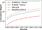
(a) $B_{K}=1$

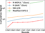
(b) $B_{K}=10$

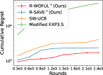
(c) $B_{K}=20$

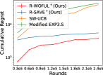
(d) $B_{K}=K^{1/3}$

Figure 1: The regret of Restarted-$\text{WeightedOFUL}^{+}$, $\text{Restarted SAVE}^{+}$, SW-UCB and Modified EXP3.S under different total rounds.

Theorem 5.5.

By using the BOB framework with Exp3 as the meta-algorithm and Restarted $\text{SAVE}^{+}$ as the base algorithm, with the candidate pool $\mathcal{P}$ for Exp3 specified as in Eq.(5.4), Eq.(5.5), Eq.(5.6), and $H=\lceil d^{\frac{2}{5}}K^{\frac{2}{5}}\rceil$, then the regret of Restarted $\text{SAVE}^{+}$-BOB (Algo.3) satisfies

$$\text{Regret}(K) =\widetilde{O}(d^{4/5}V_{K}^{2/5}B_{K}^{1/5}K^{2/5}+d^{2/3}B_{K}^{1/3}K^{2/3}+d^{2/5}K^{7/10}).$$ (5.7)

Proof.

See Appendix E for the full proof. ∎

Remark 5.6.

We discuss the regret of Algo.3 in Corollary 5.3 in the following special cases. In the case where the total variance is small, i.e., $V_{K}=\tilde{O}(1)$, assuming that $K^{2}>d$, our result becomes $\tilde{O}(d^{2/3}B_{K}^{1/3}K^{2/3}+d^{1/5}K^{7/10})$, when $d^{14}B_{K}^{10}>K$, it becomes $\tilde{O}(d^{2/3}B_{K}^{1/3}K^{2/3})$, better than all the previous results Cheung et al. (2018); Zhao et al. (2020a); Wang et al. (2023); Wei and Luo (2021). In the worst case where $V_{K}=O(K)$, our result becomes $\tilde{O}(d^{4/5}B_{K}^{1/5}K^{4/5})$.

6 Experiments

To validate the effectiveness of our methods, we conduct a series of experiments on the synthetic data.

Problem Setting Following the experimental set up in Cheung et al. (2019), we consider the 2-armed bandits setting, where the action set $\mathcal{D}_{k}=\{(1,0),(0,1)\}$, and

$$\bm{\theta}_{k}=\begin{pmatrix}0.5+\frac{3}{10}\sin(5B_{K}\pi k/K)\\ 0.5+\frac{3}{10}\sin(\pi+5B_{K}\pi k/K)\end{pmatrix}.$$

It is easy to see that the total variation budget can be bounded as $B_{K}$. At each round $k$, the $\epsilon_{k}$ satisfies the following distribution:

$$\epsilon_{k}\sim\text{Bernoulli}(0.5/k)-0.5/k.$$

We can verify that under such a distribution for $\epsilon_{k}$, the variance of the reward distribution at $k$-th round is $(1-0.5/k)\cdot 0.5/k$, and the total variance $V_{K}\sim\log K$.

Baseline algorithms We compare the proposed Restarted-$\text{WeightedOFUL}^{+}$ and $\text{Restarted SAVE}^{+}$ with SW-UCB Cheung et al. (2019) and Modified EXP3.S Besbes et al. (2014a). For Restarted-$\text{WeightedOFUL}^{+}$, we set $\lambda=1$, $\widehat{\beta}_{k}=10$, $w=1000$, and we grid search the variance parameters $\alpha$ and $\gamma$, both among values [1, 1.5, 2, 2.5, 3]. Finally we set $\alpha=1$, and $\gamma=2$. For $\text{Restarted SAVE}^{+}$ we set $w=1000$, $\widehat{\beta}_{k,\ell}=2^{-\ell+1}$, and grid search $L$ from 1 to 10 with stepsize of 1 and finally choose $L=6$. For SW-UCB, we set $\lambda=1$, $w=1000$, $\beta_{k}=10$. The Modified EXP3.S requires two parameters $\bar{\alpha}$ and $\bar{\gamma}$, and we set $\bar{\gamma}=0.01$ and $\bar{\alpha}=\frac{1}{K}$.

To test the algorithms’ performance under different total time horizons, we let $K$ vary from $3\times 10^{4}$ to $2.4\times 10^{5}$, with a stepsize of $3\times 10^{4}$, and plot the cumulative regret $\text{Regret}(K)$ for these different total time step $K$. We set $B_{K}=1,10,20,\text{and }K^{1/3}$ to observe their performance in different levels of $B_{K}$.

Result We plot the results in Figure.1, where all the empirical results are averaged over ten independent trials and the error bar is the standard error divided by $\sqrt{10}$. The results are consistent with our theoretical findings. It is evident that our algorithms significantly outperform both SW-UCB and Modified EXP3.S. Among our proposed algorithms, Restarted-$\text{WeightedOFUL}^{+}$ achieves the best performance. This can be attributed to the fact that it knows the variance and can make more informed decisions. Although $\text{Restarted SAVE}^{+}$ performed slightly worse than Restarted-$\text{WeightedOFUL}^{+}$, it still outperforms the baseline algorithms, particularly when $B_{K}=K^{1/3}$. These results highlight the superiority of our methods.

7 Conclusion and Future Work

We study non-stationary stochastic linear bandits in this work. We propose Restarted-$\text{WeightedOFUL}^{+}$ and Restarted SAVE⁺, two algorithms that utilize the dynamic variance information of the dynamic reward distribution. We show that both of our algorithms are able to achieve better dynamic regret compared with best existing results (Wei and Luo, 2021) under several parameter regimes, e.g., when the total variance $V_{K}$ is small. Experiment results backup our theoretical claim. It is worth noting there still exist gaps between our current obtained regret and the lower bound (Wei et al., 2016), and to fix such a gap leaves as our future work.

Appendix A $\text{Restarted SAVE}^{+}$-BOB

In this section, we provide the details of our proposed $\text{Restarted SAVE}^{+}$-BOB algorithm. The $\text{Restarted SAVE}^{+}$-BOB algorithm is summarized in Algo.3. In this algorithm, we divide the total time rounds $K$ into $\lceil\frac{K}{H}\rceil$ blocks, with each block having $H$ rounds (except the last block). The algorithm also labels all the $\left|\mathcal{P}\right|=\big{(}\lceil\frac{1}{3}\log_{2}K\rceil+\lceil\frac{2}{5}\log_{2}K\rceil+2\big{)}\cdot\big{(}\lceil\frac{1}{3}\log_{2}K\rceil+\lceil\frac{11}{30}\log_{2}K\rceil+2\big{)}$ candidate pairs of parameters in $\mathcal{P},$i.e., $\mathcal{P}=\{(w_{i},\alpha_{i})\}_{i=1}^{\left|\mathcal{P}\right|}$. The algorithm initializes $\{s_{j,1}\}^{\left|\mathcal{P}\right|}_{j=1}$ to be $s_{j,1}=1,\quad\forall j=0,1,\ldots,\left|\mathcal{P}\right|$, which means that at the beginning, the algorithm selects a pair from $\mathcal{P}$ uniformly at random. At the beginning of each block $i\in[\lceil K/H\rceil]$, the meta-learner (Exp3) calculates the distribution $(p_{j,i})^{\left|\mathcal{P}\right|}_{j=1}$ over the candidate set $\mathcal{P}$ by

$$p_{j,i}=(1-\gamma)\frac{s_{j,i}}{\sum_{u=1}^{\left|\mathcal{P}\right|}s_{u,i}}+\frac{\gamma}{\left|\mathcal{P}\right|+1},\quad\forall j=1,\ldots,\left|\mathcal{P}\right|\,,$$ (A.1)

where $\gamma$ is defined as

$$\gamma=\min\left\{1,\sqrt{\frac{(\left|\mathcal{P}\right|+1)\ln(\left|\mathcal{P}\right|+1)}{(e-1)\lceil K/H\rceil}}\right\}\,.$$ (A.2)

Then, the meta-learner draws a $j_{i}$ from the distribution $(p_{j,i})^{\left|\mathcal{P}\right|}_{j=1}$, and sets the pair of parameters in block $i$ to be $(w_{j_{i}},\alpha_{j_{i}})$, and runs the base algorithm Algo.2 from scratch in this block with $(w_{j_{i}},\alpha_{j_{i}})$, then feeds the cumulative reward in the block $\sum_{k=(i-1)H+1}^{\min\{i\cdot H,K\}}r_{k}$ to the meta-learner. The meta-learner rescales $\sum_{k=(i-1)H+1}^{\min\{i\cdot H,K\}}r_{k}$ to $\frac{\sum_{k=(i-1)H+1}^{\min\{i\cdot H,K\}}r_{k}}{H+R\sqrt{\frac{H}{2}\log\big{(}K(\frac{K}{H}+1)\big{)}}+\frac{2}{3}\cdot R\log\big{(}K(\frac{K}{H}+1)\big{)}}$ to make it in the range $[0,1]$ with high probability (supported by Lemma F.7). The meta-learner updates the parameter $s_{j_{i},i+1}$ to be

$$s_{j_{i},i+1}=s_{j_{i},i}\cdot\exp\left(\frac{\gamma}{(\left|\mathcal{P}\right|+1)p_{j_{i},i}}\left(\frac{1}{2}+\frac{\sum_{k=(i-1)H+1}^{\min\{i\cdot H,K\}}r_{k}}{H+R\sqrt{\frac{H}{2}\log\big{(}K(\frac{K}{H}+1)\big{)}}+\frac{2}{3}\cdot R\log\big{(}K(\frac{K}{H}+1)\big{)}}\right)\right)\,,$$ (A.3)

and keep others unchanged, i.e., $s_{u,i+1}=s_{u,i},~{}\forall u\neq j_{i}$. After that, the algorithm will go to the next block, and repeat the same process in block $i+1$.

Algorithm 3 $\text{Restarted SAVE}^{+}$-BOB

0:  total time rounds $K$; problem dimension $d$; noise upper bound $R$; $\alpha>0$; the upper bound on the $\ell_{2}$-norm of $\mathbf{a}$ in $\mathcal{D}_{k}(k\geq 1)$, i.e., $A$; the upper bound on the $\ell_{2}$-norm of $\bm{\theta}_{k}$ $(k\geq 1)$, i.e., $B$.

1:  Initialize $H=\lceil d^{\frac{2}{5}}K^{\frac{2}{5}}\rceil$; $\mathcal{P}$ as defined in Eq.(5.4), and index the $\left|\mathcal{P}\right|=\big{(}\lceil\frac{1}{3}\log_{2}K\rceil+\lceil\frac{2}{5}\log_{2}K\rceil+2\big{)}\cdot\big{(}\lceil\frac{1}{3}\log_{2}K\rceil+\lceil\frac{11}{30}\log_{2}K\rceil+2\big{)}$ items in $\mathcal{P}$, i.e., $\mathcal{P}=\{(w_{i},\alpha_{i})\}_{i=1}^{\left|\mathcal{P}\right|}$; $\gamma=\min\left\{1,\sqrt{\frac{(\left|\mathcal{P}\right|+1)\ln(\left|\mathcal{P}\right|+1)}{(e-1)\lceil K/H\rceil}}\right\}$; $\{s_{j,1}\}^{\left|\mathcal{P}\right|}_{j=1}$ is set to $s_{j,1}=1,\quad\forall j=0,1,\ldots,\left|\mathcal{P}\right|$.

2:  for $i=1,2,\ldots,\lceil K/H\rceil$ do

3:     Calculate the distribution $(p_{j,i})^{\left|\mathcal{P}\right|}_{j=1}$ by $p_{j,i}=(1-\gamma)\frac{s_{j,i}}{\sum_{u=1}^{\left|\mathcal{P}\right|}s_{u,i}}+\frac{\gamma}{\left|\mathcal{P}\right|+1},\quad\forall j=1,\ldots,\left|\mathcal{P}\right|$.

4:     Set $j_{i}\leftarrow j$ with probability $p_{j,i}$, and $(w_{i},\alpha_{i})\leftarrow(w_{i_{i}},\alpha_{j_{i}})$.

5:     Run Algo.2 from scratch in block $i$ (i.e., in rounds $k=(i-1)H+1,\ldots,\min\{i\cdot H,K\}$) with $(w,\alpha)=(w_{i},\alpha_{i})$.

6:     Update $s_{j_{i},i+1}=s_{j_{i},i}\cdot\exp\left(\frac{\gamma}{(\left|\mathcal{P}\right|+1)p_{j_{i},i}}\left(\frac{1}{2}+\frac{\sum_{k=(i-1)H+1}^{\min\{i\cdot H,K\}}r_{k}}{H+R\sqrt{\frac{H}{2}\log\big{(}K(\frac{K}{H}+1)\big{)}}+\frac{2}{3}\cdot R\log\big{(}K(\frac{K}{H}+1)\big{)}}\right)\right)$, and keep all the others unchanged, i.e., $s_{u,i+1}=s_{u,i},~{}\forall u\neq j_{i}$.

7:  end for

Appendix B Proof of Lemma 4.1

For simplicity, we denote

$$\widehat{\beta} :=12\sqrt{d\log(1+\frac{wA^{2}}{\alpha^{2}d\lambda})\log(32(\log(\frac{\gamma^{2}}{\alpha}+1)\frac{w^{2}}{\delta})}+30\log(32(\log(\frac{\gamma^{2}}{\alpha})+1)\frac{w^{2}}{\delta})\frac{R}{\gamma^{2}}+\sqrt{\lambda}B.$$ (B.1)

It is obvious that $\widehat{\beta}\geq\widehat{\beta}_{k}$ for all $k\in[K]$. We call the restart time rounds grids and denote them by $g_{1},g_{2},\ldots g_{\lceil\frac{K}{w}\rceil-1}$, where $g_{i}\%w=0$ for all $i\in[\lceil\frac{K}{w}\rceil-1]$. Let $i_{k}$ be the grid index of time round $k$, i.e., $g_{i_{k}}\leq k<g_{i_{k}+1}$.

For ease of exposition and without loss of generality, we prove the lemma for $k\in[1,w]$. We calculate the estimation difference $|\bm{a}^{\top}(\widehat{\bm{\theta}}_{k}-\bm{\theta}_{k})|$ for any $\mathbf{a}\in\mathbb{R}^{d}$, $\|\mathbf{a}\|_{2}\leq A$, $k\in[1,w]$. By definition:

$$\widehat{\bm{\theta}}_{k}=\widehat{\bm{\Sigma}}_{k}^{-1}\bm{b}_{k}=\widehat{\bm{\Sigma}}_{k}^{-1}(\sum_{t=1}^{k-1}\frac{r_{t}\mathbf{a}_{t}}{\bar{\sigma}_{t}^{2}})=\widehat{\bm{\Sigma}}_{k}^{-1}(\sum_{t=1}^{k-1}\frac{\mathbf{a}_{t}\mathbf{a}_{t}^{\top}\bm{\theta}_{t}}{\bar{\sigma}_{t}^{2}}+\sum_{t=1}^{k-1}\frac{\mathbf{a}_{t}\epsilon_{t}}{\bar{\sigma}_{t}^{2}})\,,$$ (B.2)

where $\widehat{\Sigma}_{k}=\lambda\bm{I}+\sum_{t=g_{i_{k}}}^{k-1}\frac{\mathbf{a}_{t}\mathbf{a}_{t}^{\top}}{\bar{\sigma}_{t}^{2}}$.

Then we have

$$\widehat{\bm{\theta}}_{k}-\bm{\theta}_{k}=\widehat{\bm{\Sigma}}_{k}^{-1}(\sum_{t=1}^{k-1}\frac{\mathbf{a}_{t}\mathbf{a}_{t}^{\top}}{\bar{\sigma}_{t}^{2}}(\bm{\theta}_{t}-\bm{\theta}_{k})+\sum_{t=1}^{k-1}\frac{\mathbf{a}_{t}\epsilon_{t}}{\bar{\sigma}_{t}^{2}})-\lambda\widehat{\bm{\Sigma}}_{k}^{-1}\bm{\theta}_{k}\,.$$ (B.3)

Therefore

$$|\mathbf{a}^{\top}(\widehat{\bm{\theta}}_{k}-\bm{\theta}_{k})|\leq\left|\mathbf{a}^{\top}\widehat{\bm{\Sigma}}_{k}^{-1}\sum_{t=1}^{k-1}\frac{\mathbf{a}_{t}\mathbf{a}_{t}^{\top}}{\bar{\sigma}_{t}^{2}}(\bm{\theta}_{t}-\bm{\theta}_{k})\right|+\|\mathbf{a}\|_{\widehat{\bm{\Sigma}}_{k}^{-1}}\|\sum_{t=1}^{k-1}\frac{\mathbf{a}_{t}\epsilon_{t}}{\bar{\sigma}_{t}^{2}}\|_{\widehat{\bm{\Sigma}}_{k}^{-1}}+\lambda\|\mathbf{a}\|_{\widehat{\bm{\Sigma}}_{k}^{-1}}\|\widehat{\bm{\Sigma}}_{k}^{-\frac{1}{2}}\bm{\theta}_{k}\|_{2}\,,$$ (B.4)

where we use the Cauchy-Schwarz inequality.

For the first term, we have that for any $k\in[1,w]$

$$\left|\mathbf{a}^{\top}\widehat{\bm{\Sigma}}_{k}^{-1}\sum_{t=1}^{k}\frac{\mathbf{a}_{t}\mathbf{a}_{t}^{\top}}{\bar{\sigma}_{t}^{2}}(\bm{\theta}_{t}-\bm{\theta}_{k})\right| \leq\sum_{t=1}^{k-1}|\mathbf{a}^{\top}\widehat{\bm{\Sigma}}_{k}^{-1}\frac{\mathbf{a}_{t}}{\bar{\sigma}_{t}}|\cdot|\frac{\mathbf{a}_{t}}{\bar{\sigma}_{t}}^{\top}(\sum_{s=t}^{k-1}(\bm{\theta}_{s}-\bm{\theta}_{s+1}))|$$ (triangle inequality )

$$\leq\sum_{t=1}^{k-1}|\mathbf{a}^{\top}\widehat{\bm{\Sigma}}_{k}^{-1}\frac{\mathbf{a}_{t}}{\bar{\sigma}_{t}}|\cdot\|\frac{\mathbf{a}_{t}}{\bar{\sigma}_{t}}\|_{2}\cdot\|\sum_{s=t}^{k-1}(\bm{\theta}_{s}-\bm{\theta}_{s+1})\|_{2}$$ (Cauchy-Schwarz)

$$\leq\frac{A}{\alpha}\sum_{t=1}^{k-1}|\mathbf{a}^{\top}\widehat{\bm{\Sigma}}_{k}^{-1}\frac{\mathbf{a}_{t}}{\bar{\sigma}_{t}}|\cdot\|\sum_{s=t}^{k-1}(\bm{\theta}_{s}-\bm{\theta}_{s+1})\|_{2} \|\mathbf{a}_{t}\|\leq A \bar{\sigma}_{t}\geq\alpha$$ (, )

$$\leq\frac{A}{\alpha}\sum_{s=1}^{k-1}\sum_{t=1}^{s}|\mathbf{a}^{\top}\widehat{\bm{\Sigma}}_{k}^{-1}\frac{\mathbf{a}_{t}}{\bar{\sigma}_{t}}|\cdot\|\bm{\theta}_{s}-\bm{\theta}_{s+1}\|_{2} \sum_{t=1}^{k-1}\sum_{s=t}^{k-1}=\sum_{s=1}^{k-1}\sum_{t=1}^{s}$$ ()

$$\leq\frac{A}{\alpha}\sum_{s=1}^{k-1}\sqrt{\bigg{[}\sum_{t=1}^{s}\mathbf{a}^{\top}\widehat{\bm{\Sigma}}_{k}^{-1}\mathbf{a}\bigg{]}\cdot\biggl{[}\sum_{t=1}^{s}\frac{\mathbf{a}_{t}}{\bar{\sigma}_{t}}^{\top}\widehat{\bm{\Sigma}}_{k}^{-1}\frac{\mathbf{a}_{t}}{\bar{\sigma}_{t}}\bigg{]}}\cdot||\bm{\theta}_{s}-\bm{\theta}_{s+1}||_{2}$$ (Cauchy-Schwarz)

$$\leq\frac{A}{\alpha}\sum_{s=1}^{k-1}\sqrt{\bigg{[}\sum_{t=1}^{s}\mathbf{a}^{\top}\widehat{\bm{\Sigma}}_{k}^{-1}\mathbf{a}\bigg{]}\cdot d}\cdot||\bm{\theta}_{s}-\bm{\theta}_{s+1}||_{2} (\star)$$ ()

$$\leq\frac{A\|\mathbf{a}\|_{2}}{\alpha}\sqrt{d}\sum_{s=1}^{k-1}\sqrt{\frac{\sum_{t=1}^{k-1}1}{\lambda}}\cdot||\bm{\theta}_{s}-\bm{\theta}_{s+1}||_{2} \lambda_{\max}(\widehat{\bm{\Sigma}}_{k}^{-1})\leq\frac{1}{\lambda}$$ ()

$$\leq\frac{A^{2}}{\alpha}\sqrt{\frac{dw}{\lambda}}\sum_{s=1}^{k-1}||\bm{\theta}_{s}-\bm{\theta}_{s+1}||_{2}\,,$$ (B.5)

where the inequality $(\star)$ follows from the fact that $\sum_{t=1}^{s}\frac{\mathbf{a}_{t}}{\bar{\sigma}_{t}}^{\top}\widehat{\bm{\Sigma}}_{k}^{-1}\frac{\mathbf{a}_{t}}{\bar{\sigma}_{t}}\leq d$ that can be proved as follows. We have $\sum_{t=1}^{k-1}\frac{\mathbf{a}_{t}}{\bar{\sigma}_{t}}^{\top}\widehat{\bm{\Sigma}}_{k}^{-1}\frac{\mathbf{a}_{t}}{\bar{\sigma}_{t}}=\sum_{t=1}^{k-1}\text{tr}\left(\frac{\mathbf{a}_{t}}{\bar{\sigma}_{t}}^{\top}\widehat{\bm{\Sigma}}_{k}^{-1}\frac{\mathbf{a}_{t}}{\bar{\sigma}_{t}}\right)=\text{tr}\left(\widehat{\bm{\Sigma}}_{k}^{-1}\sum_{t=1}^{k-1}\frac{\mathbf{a}_{t}}{\bar{\sigma}_{t}}\frac{\mathbf{a}_{t}}{\bar{\sigma}_{t}}^{\top}\right)$. Given the eigenvalue decomposition $\sum_{t=1}^{k-1}\frac{\mathbf{a}_{t}}{\bar{\sigma}_{t}}\frac{\mathbf{a}_{t}}{\bar{\sigma}_{t}}^{\top}=\text{diag}(\lambda_{1},\ldots,\lambda_{d})^{\top}$, we have $\widehat{\bm{\Sigma}}_{k}=\text{diag}(\lambda_{1}+\lambda,\ldots,\lambda_{d}+\lambda)^{\top}$, and $\text{tr}\left(\widehat{\bm{\Sigma}}_{k}^{-1}\sum_{t=1}^{k-1}\frac{\mathbf{a}_{t}}{\bar{\sigma}_{t}}\frac{\mathbf{a}_{t}}{\bar{\sigma}_{t}}^{\top}\right)=\sum_{i=1}^{d}\frac{\lambda_{j}}{\lambda_{j}+\lambda}\leq d$.

For the second term, by the assumption on $\epsilon_{k}$, we know that

$$|\epsilon_{k}/\bar{\sigma}_{k}|\leq R/\alpha,$$

$$|\epsilon_{k}/\bar{\sigma}_{k}|\cdot\min\{1,\|\mathbf{a}_{k}/\bar{\sigma}_{k}\|_{\widehat{\bm{\Sigma}}_{k}^{-1}}\}\leq R\|\mathbf{a}_{k}\|_{\widehat{\bm{\Sigma}}_{k}^{-1}}/\bar{\sigma}_{k}^{2}\leq R/\gamma^{2},$$

$$\mathbb{E}[\epsilon_{k}|\mathbf{a}_{1:k},\epsilon_{1:k-1}]=0,\ \mathbb{E}[(\epsilon_{k}/\bar{\sigma}_{k})^{2}|\mathbf{a}_{1:k},\epsilon_{1:k-1}]\leq 1,\ \|\mathbf{a}_{k}/\bar{\sigma}_{k}\|_{2}\leq A/\alpha,$$

Therefore, setting $\mathcal{G}_{k}=\sigma(\mathbf{a}_{1:k},\epsilon_{1:k-1})$, and using that $\sigma_{k}$ is $\mathcal{G}_{k}$-measurable, applying Theorem F.1 to $(\bm{x}_{k},\eta_{k})=(\bm{a}_{k}/\bar{\sigma}_{k},\epsilon_{k}/\bar{\sigma}_{k})$ with $\epsilon=R/\gamma^{2}$ , we get that with probability at least $1-\delta$, for all $k\in[1,w]$,

$$\|\sum_{t=1}^{k-1}\frac{\mathbf{a}_{t}\epsilon_{t}}{\bar{\sigma}_{t}^{2}}\|_{\widehat{\bm{\Sigma}}_{k}^{-1}}\leq 12\sqrt{d\log(1+\frac{(k\%w)A^{2}}{\alpha^{2}d\lambda})\log(32(\log(\frac{\gamma^{2}}{\alpha}+1)\frac{(k\%w)^{2}}{\delta})}+30\log(32(\log(\frac{\gamma^{2}}{\alpha})+1)\frac{(k\%w)^{2}}{\delta})\frac{R}{\gamma^{2}}.$$ (B.6)

For the last term

$$\lambda\|\mathbf{a}\|_{\widehat{\bm{\Sigma}}_{k}^{-1}}\|\widehat{\bm{\Sigma}}_{k}^{-\frac{1}{2}}\bm{\theta}_{k}\|_{2}\leq\lambda\|\mathbf{a}\|_{\widehat{\bm{\Sigma}}_{k}^{-1}}\|\widehat{\bm{\Sigma}}_{k}^{-\frac{1}{2}}\|_{2}\|\bm{\theta}_{k}\|_{2}\leq\lambda\|\mathbf{a}\|_{\widehat{\bm{\Sigma}}_{k}^{-1}}\frac{1}{\sqrt{\lambda_{\text{min}}(\widehat{\bm{\Sigma}}_{k})}}\|\bm{\theta}_{k}\|_{2}\leq\sqrt{\lambda}B\|\mathbf{a}\|_{\widehat{\bm{\Sigma}}_{k}^{-1}}\,,$$ (B.7)

where we use the fact that $\lambda_{\text{min}}(\widehat{\bm{\Sigma}}_{k})\geq\lambda$.

Therefore, with probabilty at least $1-\delta$, we have

$$|\mathbf{a}^{\top}(\widehat{\bm{\theta}}_{k}-\bm{\theta}_{k})| \leq\frac{A^{2}}{\alpha}\sqrt{\frac{dw}{\lambda}}\sum_{t=1}^{k-1}\|\bm{\theta}_{t}-\bm{\theta}_{t+1}\|_{2}$$

$$\quad+\|\mathbf{a}\|_{\widehat{\bm{\Sigma}}_{k}^{-1}}\bigg{(}12\sqrt{d\log(1+\frac{(k\%w)A^{2}}{\alpha^{2}d\lambda})\log(32(\log(\frac{\gamma^{2}}{\alpha}+1)\frac{(k\%w)^{2}}{\delta})}$$

$$\quad+30\log(32(\log(\frac{\gamma^{2}}{\alpha})+1)\frac{(k\%w)^{2}}{\delta})\frac{R}{\gamma^{2}}+\sqrt{\lambda}B\bigg{)}$$

$$=\frac{A^{2}}{\alpha}\sqrt{\frac{dw}{\lambda}}\sum_{t=1}^{k-1}\|\bm{\theta}_{t}-\bm{\theta}_{t+1}\|_{2}+\widehat{\beta}_{k}\|\mathbf{a}\|_{\widehat{\bm{\Sigma}}_{k}^{-1}}\,,$$ (B.8)

where $\widehat{\beta}_{k}$ is defined in Eq.(4.3).

Appendix C Proof for Theorem 4.2

For simplicity of analysis, we only analyze the regret over the first grid, i.e., we try to analyze $\text{Regret}(\widetilde{K})$ for $\widetilde{K}\in[1,w]$. Denote $\mathcal{E}_{1}$ as the event when Lemma 4.1 holds. Therefore, under event $\mathcal{E}_{1}$, for any $\widetilde{K}\in[1,w]$, the regret can be bounded by

$$\text{Regret}(\widetilde{K}) =\sum_{k=1}^{\widetilde{K}}\big{[}\langle\mathbf{a}_{k}^{*}-\mathbf{a}_{k},\bm{\theta}_{k}\rangle\big{]}$$

$$=\sum_{k=1}^{\widetilde{K}}\big{[}\langle\mathbf{a}_{k}^{*},\bm{\theta}_{k}-\widehat{\bm{\theta}}_{k}\rangle+(\langle\mathbf{a}_{k}^{*},\widehat{\bm{\theta}}_{k}\rangle+\widehat{\beta}_{k}\|\mathbf{a}_{k}^{*}\|_{\widehat{\bm{\Sigma}}_{k}^{-1}})-(\langle\mathbf{a}_{k},\widehat{\bm{\theta}}_{k}\rangle+\widehat{\beta}_{k}\|\mathbf{a}_{k}\|_{\widehat{\bm{\Sigma}}_{k}^{-1}})+\langle\mathbf{a}_{k},\widehat{\bm{\theta}}_{k}-\bm{\theta}_{k}\rangle$$

$$\quad+\widehat{\beta}_{k}\|\mathbf{a}_{k}\|_{\widehat{\bm{\Sigma}}_{k}^{-1}}-\widehat{\beta}_{k}\|\mathbf{a}_{k}^{*}\|_{\widehat{\bm{\Sigma}}_{k}^{-1}}\big{]}$$

$$\leq\frac{2A^{2}}{\alpha}\sqrt{\frac{dw}{\lambda}}\sum_{k=1}^{\widetilde{K}}\sum_{t=1}^{k-1}\|\bm{\theta}_{t}-\bm{\theta}_{t+1}\|_{2}+2\sum_{k=1}^{\widetilde{K}}\min\Big{\{}1,\widehat{\beta}_{k}\|\mathbf{a}_{k}\|_{\widehat{\bm{\Sigma}}_{k}^{-1}}\Big{\}}\,,$$ (C.1)

where in the last inequality we use the definition of event $\mathcal{E}_{1}$, the arm selection rule in Line 7 of Algo.8, and $0\leq\langle\mathbf{a}_{k}^{*},\bm{\theta}^{*}\rangle-\langle\mathbf{a}_{k},\bm{\theta}^{*}\rangle\leq 2$.

Then we will bound the two terms in Eq.(C.1).

For the first term, we have

$$\frac{2A^{2}}{\alpha}\sqrt{\frac{dw}{\lambda}}\sum_{k=1}^{\widetilde{K}}\sum_{t=1}^{k-1}\|\bm{\theta}_{t}-\bm{\theta}_{t+1}\|_{2}$$

$$=\frac{2A^{2}}{\alpha}\sqrt{\frac{dw}{\lambda}}\sum_{t=1}^{\widetilde{K}-1}\sum_{k=t}^{\widetilde{K}}\|\bm{\theta}_{t}-\bm{\theta}_{t+1}\|_{2}$$

$$\leq\frac{2A^{2}}{\alpha}\sqrt{\frac{dw}{\lambda}}w\sum_{t=1}^{\widetilde{K}-1}\|\bm{\theta}_{t}-\bm{\theta}_{t+1}\|_{2}\,.$$ (C.2)

To bound the second term in Eq.(C.1), we decompose the set $[\widetilde{K}]$ into a union of two disjoint subsets $[K]=\mathcal{I}_{1}\cup\mathcal{I}_{2}$.

$$\mathcal{I}_{1}=\Big{\{}k\in[\widetilde{K}]:\|\frac{\mathbf{a}_{k}}{\bar{\sigma}_{k}}\|_{\widehat{\bm{\Sigma}}_{k}^{-1}}\geq 1\Big{\}},\ \mathcal{I}_{2}=\Big{\{}k\in[\widetilde{K}]:\|\frac{\mathbf{a}_{k}}{\bar{\sigma}_{k}}\|_{\widehat{\bm{\Sigma}}_{k}^{-1}}<1\Big{\}}.$$ (C.3)

Then the following upper bound of $|\mathcal{I}_{1}|$ holds:

$$|\mathcal{I}_{1}| =\sum_{k\in\mathcal{I}_{1}}\min\Big{\{}1,\|\frac{\mathbf{a}_{k}}{\bar{\sigma}_{k}}\|_{\widehat{\bm{\Sigma}}_{k}^{-1}}^{2}\Big{\}}$$

$$\leq\sum_{k=1}^{\widetilde{K}}\min\Big{\{}1,\|\frac{\mathbf{a}_{k}}{\bar{\sigma}_{k}}\|_{\widehat{\bm{\Sigma}}_{k}^{-1}}^{2}\Big{\}}$$

$$\leq 2d\iota,$$ (C.4)

where $\iota=\log(1+\frac{wA^{2}}{d\lambda\alpha^{2}})$, the first equality holds since $\|\frac{\mathbf{x}_{k}}{\bar{\sigma}_{k}}\|_{\widehat{\bm{\Sigma}}_{k}^{-1}}\geq 1$ for $k\in\mathcal{I}_{1}$, the last inequality holds due to Lemma F.2 together with the fact $\|\frac{\mathbf{a}_{k}}{\bar{\sigma}_{k}}\|_{2}\leq\frac{A}{\alpha}$ since $\bar{\sigma}_{k}\geq\alpha$ and $\|\mathbf{a}_{k}\|_{2}\leq A$.

Then, we have

$$\sum_{k=1}^{\widetilde{K}}\min\Big{\{}1,\widehat{\beta}_{k}\|\mathbf{a}_{k}\|_{\widehat{\bm{\Sigma}}_{k}^{-1}}\Big{\}}$$

$$=\sum_{k\in\mathcal{I}_{1}}\min\Big{\{}1,\bar{\sigma}_{k}\widehat{\beta}_{k}\|\frac{\mathbf{a}_{k}}{\bar{\sigma}_{k}}\|_{\widehat{\bm{\Sigma}}_{k}^{-1}}\Big{\}}+\sum_{k\in\mathcal{I}_{2}}\min\Big{\{}1,\bar{\sigma}_{k}\widehat{\beta}_{k}\|\frac{\mathbf{a}_{k}}{\bar{\sigma}_{k}}\|_{\widehat{\bm{\Sigma}}_{k}^{-1}}\Big{\}}$$

$$\leq\bigg{[}\sum_{k\in\mathcal{I}_{1}}1\bigg{]}+\sum_{k\in\mathcal{I}_{2}}\bar{\sigma}_{k}\widehat{\beta}_{k}\|\frac{\mathbf{a}_{k}}{\bar{\sigma}_{k}}\|_{\widehat{\bm{\Sigma}}_{k}^{-1}}$$

$$\leq 2d\iota+\widehat{\beta}\sum_{k\in\mathcal{I}_{2}}\bar{\sigma}_{k}\|\frac{\mathbf{a}_{k}}{\bar{\sigma}_{k}}\|_{\widehat{\bm{\Sigma}}_{k}^{-1}},$$ (C.5)

where the first inequality holds since $\min\{1,x\}\leq 1$ and also $\min\{1,x\}\leq x$, the second inequality holds by Eq.(C.4), and the fact the $\widehat{\beta}\geq\widehat{\beta}_{k}$ for all $k\in[K]$ ($\widehat{\beta}$ is defined in Eq.(B.1)). Next we further bound the second summation term in (C.5). We decompose $\mathcal{I}_{2}=\mathcal{J}_{1}\cup\mathcal{J}_{2}$, where

$$\mathcal{J}_{1}=\bigg{\{}k\in\mathcal{I}_{2}:\bar{\sigma}_{k}=\sigma_{k}\cup\bar{\sigma}_{k}=\alpha\bigg{\}},\ \mathcal{J}_{2}=\bigg{\{}k\in\mathcal{I}_{2}:\bar{\sigma}_{k}=\gamma\sqrt{\|\mathbf{a}_{k}\|_{\widehat{\bm{\Sigma}}_{k}^{-1}}}\bigg{\}}.$$

Then $\sum_{k\in\mathcal{I}_{2}}\bar{\sigma}_{k}\|\frac{\mathbf{a}_{k}}{\bar{\sigma}_{k}}\|_{\widehat{\bm{\Sigma}}_{k}^{-1}}=\sum_{k\in\mathcal{J}_{1}}\bar{\sigma}_{k}\|\frac{\mathbf{a}_{k}}{\bar{\sigma}_{k}}\|_{\widehat{\bm{\Sigma}}_{k}^{-1}}$+$\sum_{k\in\mathcal{J}_{2}}\bar{\sigma}_{k}\|\frac{\mathbf{a}_{k}}{\bar{\sigma}_{k}}\|_{\widehat{\bm{\Sigma}}_{k}^{-1}}$. First, for $k\in\mathcal{J}_{1}$, we have

$$\sum_{k\in\mathcal{J}_{1}}\bar{\sigma}_{k}\|\frac{\mathbf{a}_{k}}{\bar{\sigma}_{k}}\|_{\widehat{\bm{\Sigma}}_{k}^{-1}} \leq\sum_{k\in\mathcal{J}_{1}}(\sigma_{k}+\alpha)\min\bigg{\{}1,\|\frac{\mathbf{a}_{k}}{\bar{\sigma}_{k}}\|_{\widehat{\bm{\Sigma}}_{k}^{-1}}\bigg{\}}$$

$$\leq\sqrt{\sum_{k=1}^{\widetilde{K}}(\sigma_{k}+\alpha)^{2}}\sqrt{\sum_{k=1}^{\widetilde{K}}\min\bigg{\{}1,\|\frac{\mathbf{a}_{k}}{\bar{\sigma}_{k}}\|_{\widehat{\bm{\Sigma}}_{k}^{-1}}\bigg{\}}^{2}}$$

$$\leq\sqrt{2\sum_{k=1}^{\widetilde{K}}(\sigma_{k}^{2}+\alpha^{2})}\sqrt{\sum_{k=1}^{\widetilde{K}}\min\bigg{\{}1,\|\frac{\mathbf{a}_{k}}{\bar{\sigma}_{k}}\|_{\widehat{\bm{\Sigma}}_{k}^{-1}}^{2}\bigg{\}}}$$

$$\leq 2\sqrt{\sum_{k=1}^{\widetilde{K}}\sigma_{k}^{2}+{\widetilde{K}}\alpha^{2}}\sqrt{d\iota}\,,$$ (C.6)

where the first inequality holds since $\bar{\sigma}_{k}\leq\sigma_{k}+\alpha$ for $k\in\mathcal{J}_{1}$ and $\|\frac{\mathbf{a}_{k}}{\bar{\sigma}_{k}}\|_{\widehat{\bm{\Sigma}}_{k}^{-1}}\leq 1$ since $k\in\mathcal{J}_{1}\subseteq\mathcal{I}_{2}$, the second inequality holds by Cauchy-Schwarz inequality, the third inequality holds due to $(a+b)^{2}\leq 2(a^{2}+b^{2})$, and the last inequality holds due to Lemma F.2.

Finally we bound the summation for $k\in\mathcal{J}_{2}$. When $k\in\mathcal{J}_{2}$, we have $\bar{\sigma}_{k}=\gamma^{2}\|\frac{\mathbf{a}_{k}}{\bar{\sigma}_{k}}\|_{\widehat{\Sigma}_{k}^{-1}}$. Therefore we have

$$\sum_{k\in\mathcal{J}_{2}}\bar{\sigma}_{k}\|\frac{\mathbf{a}_{k}}{\bar{\sigma}_{k}}\|_{\widehat{\bm{\Sigma}}_{k}^{-1}} =\sum_{k\in\mathcal{J}_{2}}\gamma^{2}\|\frac{\mathbf{a}_{k}}{\bar{\sigma}_{k}}\|_{\widehat{\bm{\Sigma}}_{k}^{-1}}^{2}$$

$$\leq\sum_{k=1}^{\widetilde{K}}\gamma^{2}\min\bigg{\{}1,\|\frac{\mathbf{a}_{k}}{\bar{\sigma}_{k}}\|^{2}_{\widehat{\bm{\Sigma}}_{k}^{-1}}\bigg{\}}$$

$$\leq 2\gamma^{2}d\iota\,,$$ (C.7)

where in the first inequality we use the fact that $\|\frac{\mathbf{a}_{k}}{\bar{\sigma}_{k}}\|_{\widehat{\bm{\Sigma}}_{k}^{-1}}\leq 1$ since $k\in\mathcal{J}_{2}\subseteq\mathcal{I}_{2}$, and in the last inequality we use Lemma F.2.

Therefore, with Eq.(C.1), Eq.(C.2), Eq.(C.5), Eq.(C.6), Eq.(C.7), we can get the regret upper bound for $\widetilde{K}\in[1,w]$

$$\text{Regret}(\widetilde{K}) \leq\frac{2A^{2}w^{\frac{3}{2}}}{\alpha}\sqrt{\frac{d}{\lambda}}\sum_{k=1}^{\widetilde{K}-1}\|\bm{\theta}_{k}-\bm{\theta}_{k+1}\|_{2}+4\widehat{\beta}\sqrt{d\iota}\sqrt{\sum_{k\in[\widetilde{K}]}\sigma_{k}^{2}+w\alpha^{2}}+4d\iota\gamma^{2}\widehat{\beta}+4d\iota\,.$$ (C.8)

Therefore, by the same deduction, we can get that

$$\text{Regret}([g_{i},g_{i+1}]) \leq\frac{2A^{2}w^{\frac{3}{2}}}{\alpha}\sqrt{\frac{d}{\lambda}}\sum_{k=g_{i}}^{g_{i+1}-1}\|\bm{\theta}_{k}-\bm{\theta}_{k+1}\|_{2}+4\widehat{\beta}\sqrt{d\iota}\sqrt{\sum_{k=g_{i}}^{g_{i+1}}\sigma_{k}^{2}+w\alpha^{2}}+4d\iota\gamma^{2}\widehat{\beta}+4d\iota\,,$$ (C.9)

where we use $\text{Regret}([g_{i},g_{i+1}])$ to denote the regret accumulated in the time period $[g_{i},g_{i+1}]$.

Finally, without loss of generality, we assume $K\%w=0$. Then we have

$$\text{Regret}(\widetilde{K}) =\sum_{i=0}^{\frac{K}{w}-1}\text{Regret}([g_{i},g_{i+1}])$$

$$\leq\frac{2A^{2}w^{\frac{3}{2}}}{\alpha}\sqrt{\frac{d}{\lambda}}\sum_{i=0}^{\frac{K}{w}-1}\sum_{k=g_{i}}^{g_{i+1}-1}\|\bm{\theta}_{k}-\bm{\theta}_{k+1}\|_{2}+4\widehat{\beta}\sqrt{d\iota}\sum_{i=0}^{\frac{K}{w}-1}\sqrt{\sum_{k=g_{i}}^{g_{i+1}}\sigma_{k}^{2}+w\alpha^{2}}+\frac{4d\iota\gamma^{2}\widehat{\beta}K}{w}+\frac{4dK\iota}{w}$$

$$\leq\frac{2A^{2}w^{\frac{3}{2}}}{\alpha}\sqrt{\frac{d}{\lambda}}\sum_{k=1}^{K-1}\|\bm{\theta}_{k}-\bm{\theta}_{k+1}\|_{2}+4\widehat{\beta}\sqrt{d\iota}\sqrt{\frac{K}{w}\sum_{i=0}^{\frac{K}{w}-1}(\sum_{k=g_{i}}^{g_{i+1}}\sigma_{k}^{2}+w\alpha^{2})}+\frac{4d\iota\gamma^{2}\widehat{\beta}K}{w}+\frac{4dK\iota}{w}$$

$$\leq\frac{2A^{2}w^{\frac{3}{2}}B_{K}}{\alpha}\sqrt{\frac{d}{\lambda}}+4\widehat{\beta}\sqrt{\frac{Kd\iota}{w}}\sqrt{\sum_{k=1}^{K}\sigma_{k}^{2}+K\alpha^{2}}+\frac{4d\iota\gamma^{2}\widehat{\beta}K}{w}+\frac{4dK\iota}{w}\,,$$

where in the second inequality we use Cauchy-Schwarz inequality, and the last inequality holds due to $\sum_{k\in[K-1]}\|\bm{\theta}_{k}-\bm{\theta}_{k+1}\|_{2}\leq B_{K}$.

Appendix D Proof for Theorem 5.1

Recall that we call the restart time rounds grids and denote them by $g_{1},g_{2},\ldots g_{\lceil\frac{K}{w}\rceil-1}$, where $g_{i}\%w=0$ for all $i\in[\lceil\frac{K}{w}\rceil-1]$. Let $i_{k}$ be the grid index of time round $k$, i.e., $g_{i_{k}}\leq k<g_{i_{k}+1}$. We denote $\widehat{\Psi}_{k,\ell}:=\{t:t\in[g_{i_{k}},k-1],\ell_{t}=\ell\}$.

For simplicity of analysis, we first try to bound the regret over the first grid, i.e., we try to analyze $\text{Regret}(\widetilde{K})$ for $\widetilde{K}\in[1,w]$. Note that in this case, for any $k\in[\widetilde{K}]$ with $\widetilde{K}\in[1,w]$, we have $g_{i_{k}}=1$, so $\widehat{\Psi}_{k,\ell}:=\{t:t\in[1,k-1],\ell_{t}=\ell\}$.

First, we calculate the estimation difference $|\bm{a}^{\top}(\widehat{\bm{\theta}}_{k,\ell}-\bm{\theta}_{k})|$ for any $\mathbf{a}\in\mathbb{R}^{d}$, $\|\mathbf{a}\|_{2}\leq A$. Recall that by definition, $\widehat{\Sigma}_{k,\ell}=2^{-2\ell}\bm{I}+\sum_{t\in\widehat{\Psi}_{k,\ell}}w_{t}^{2}\mathbf{a}_{t}\mathbf{a}_{t}^{\top}$, $\widehat{\bm{b}}_{k,\ell}=\sum_{t\in\widehat{\Psi}_{k,\ell}}w_{t}^{2}r_{t}\mathbf{a}_{t}$, and

$$\widehat{\bm{\theta}}_{k,\ell} =\widehat{\Sigma}_{k,\ell}^{-1}\widehat{\bm{b}}_{k,\ell}=\widehat{\Sigma}_{k,\ell}^{-1}(\sum_{t\in\widehat{\Psi}_{k,\ell}}w_{t}^{2}r_{t}\mathbf{a}_{t})=\widehat{\Sigma}_{k,\ell}^{-1}(\sum_{t\in\widehat{\Psi}_{k,\ell}}w_{t}^{2}\mathbf{a}_{t}\mathbf{a}_{t}^{\top}\bm{\theta}_{t}+\sum_{t\in\widehat{\Psi}_{k,\ell}}w_{t}^{2}\mathbf{a}_{t}\epsilon_{t})\,.$$

Then we have

$$\widehat{\bm{\theta}}_{k,\ell}-\bm{\theta}_{k}=\widehat{\Sigma}_{k,\ell}^{-1}(\sum_{t\in\widehat{\Psi}_{k,\ell}}w_{t}^{2}\mathbf{a}_{t}\mathbf{a}_{t}^{\top}(\bm{\theta}_{t}-\bm{\theta}_{k})+\sum_{t\in\widehat{\Psi}_{k,\ell}}w_{t}^{2}\mathbf{a}_{t}\epsilon_{t})-2^{-2\ell}\widehat{\Sigma}_{k,\ell}^{-1}\bm{\theta}_{k}\,.$$ (D.1)

Therefore, we can get

$$|\mathbf{a}^{\top}(\widehat{\bm{\theta}}_{k,\ell}-\bm{\theta}_{k})|\leq\left|\mathbf{a}^{\top}\widehat{\bm{\Sigma}}_{k,\ell}^{-1}\sum_{t\in\widehat{\Psi}_{k,\ell}}w_{t}^{2}{\mathbf{a}_{t}\mathbf{a}_{t}^{\top}}(\bm{\theta}_{t}-\bm{\theta}_{k})\right|+\|\mathbf{a}\|_{\widehat{\bm{\Sigma}}_{k,\ell}^{-1}}\|\sum_{t\in\widehat{\Psi}_{k,\ell}}w_{t}^{2}{\mathbf{a}_{t}\epsilon_{t}}\|_{\widehat{\bm{\Sigma}}_{k,\ell}^{-1}}+2^{-2\ell}\|\mathbf{a}\|_{\widehat{\bm{\Sigma}}_{k,\ell}^{-1}}\|\widehat{\bm{\Sigma}}_{k,\ell}^{-\frac{1}{2}}\bm{\theta}_{k}\|_{2}\,,$$ (D.2)

where we use the Cauchy-Schwarz inequality.

For the first term, we have that for any $k\in[1,w]$

$$\left|\mathbf{a}^{\top}\widehat{\bm{\Sigma}}_{k,\ell}^{-1}\sum_{t\in\widehat{\Psi}_{k,\ell}}w_{t}^{2}{\mathbf{a}_{t}\mathbf{a}_{t}^{\top}}(\bm{\theta}_{t}-\bm{\theta}_{k})\right| \leq\sum_{t\in\widehat{\Psi}_{k,\ell}}|\mathbf{a}^{\top}\bm{\Sigma}_{k,\ell}^{-1}w_{t}\mathbf{a}_{t}|\cdot|w_{t}\mathbf{a}_{t}^{\top}(\sum_{s=t}^{k-1}(\bm{\theta}_{s}-\bm{\theta}_{s+1}))|$$ (triangle inequality )

$$\leq\sum_{t\in\widehat{\Psi}_{k,\ell}}|\mathbf{a}^{\top}\bm{\Sigma}_{k,\ell}^{-1}w_{t}{\mathbf{a}_{t}}|\cdot\|w_{t}\mathbf{a}_{t}\|_{2}\cdot\|\sum_{s=t}^{k-1}(\bm{\theta}_{s}-\bm{\theta}_{s+1})\|_{2}$$ (Cauchy-Schwarz)

$$\leq{A}\sum_{t\in\widehat{\Psi}_{k,\ell}}|\mathbf{a}^{\top}\widehat{\bm{\Sigma}}_{k,\ell}^{-1}w_{t}{\mathbf{a}_{t}}|\cdot\|\sum_{s=t}^{k-1}(\bm{\theta}_{s}-\bm{\theta}_{s+1})\|_{2} \|\mathbf{a}_{t}\|\leq A w_{t}=\frac{2^{-\ell_{t}}}{\|\mathbf{a}_{t}\|_{\widehat{\Sigma}_{t,\ell_{t}}^{-1}}}\leq 1$$ (, )

$$\leq{A}\sum_{s=1}^{k-1}\sum_{t\in\widehat{\Psi}_{k,\ell}}|\mathbf{a}^{\top}\widehat{\bm{\Sigma}}_{k,\ell}^{-1}w_{t}{\mathbf{a}_{t}}|\cdot\|\bm{\theta}_{s}-\bm{\theta}_{s+1}\|_{2}$$

$$\leq{A}\sum_{s=1}^{k-1}\sqrt{\bigg{[}\sum_{t\in\widehat{\Psi}_{k,\ell}}\mathbf{a}^{\top}\widehat{\bm{\Sigma}}_{k,\ell}^{-1}\mathbf{a}\bigg{]}\cdot\biggl{[}\sum_{t\in\widehat{\Psi}_{k,\ell}}w_{t}{\mathbf{a}_{t}}^{\top}\widehat{\bm{\Sigma}}_{k,\ell}^{-1}w_{t}{\mathbf{a}_{t}}\bigg{]}}\cdot||\bm{\theta}_{s}-\bm{\theta}_{s+1}||_{2}$$ (Cauchy-Schwarz)

$$\leq{A}\sum_{s=1}^{k-1}\sqrt{\bigg{[}\sum_{t\in\widehat{\Psi}_{k,\ell}}\mathbf{a}^{\top}\widehat{\bm{\Sigma}}_{k,\ell}^{-1}\mathbf{a}\bigg{]}\cdot d}\cdot||\bm{\theta}_{s}-\bm{\theta}_{s+1}||_{2} (\star)$$ ()

$$\leq{A}\|\mathbf{a}\|_{2}\sqrt{d}\sum_{s=1}^{k-1}\sqrt{2^{2\ell}{\sum_{t\in\widehat{\Psi}_{k,\ell}}1}}\cdot||\bm{\theta}_{s}-\bm{\theta}_{s+1}||_{2} \lambda_{\max}(\widehat{\bm{\Sigma}}_{k,\ell}^{-1})\leq\frac{1}{2^{-2\ell}}=2^{2\ell}$$ ()

$$\leq{A^{2}}2^{\ell}\sqrt{{dw}}\sum_{s=1}^{k-1}||\bm{\theta}_{s}-\bm{\theta}_{s+1}||_{2}\,,$$ (D.3)

where the inequality $(\star)$ follows from the fact that $\sum_{t\in\widehat{\Psi}_{k,\ell}}w_{t}{\mathbf{a}_{t}}^{\top}\widehat{\bm{\Sigma}}_{k,\ell}^{-1}w_{t}{\mathbf{a}_{t}}\leq d$ that can be proved as follows. We have $\sum_{t\in\widehat{\Psi}_{k,\ell}}w_{t}{\mathbf{a}_{t}}^{\top}\widehat{\bm{\Sigma}}_{k,\ell}^{-1}w_{t}{\mathbf{a}_{t}}=\sum_{t\in\widehat{\Psi}_{k,\ell}}\text{tr}\left(w_{t}{\mathbf{a}_{t}}^{\top}\widehat{\bm{\Sigma}}_{k,\ell}^{-1}w_{t}{\mathbf{a}_{t}}\right)=\text{tr}\left(\widehat{\bm{\Sigma}}_{k,\ell}^{-1}\sum_{t\in\widehat{\Psi}_{k,\ell}}w_{t}^{2}{\mathbf{a}_{t}}{\mathbf{a}_{t}}^{\top}\right)$. Given the eigenvalue decomposition $\sum_{t\in\widehat{\Psi}_{k,\ell}}w_{t}^{2}{\mathbf{a}_{t}}{\mathbf{a}_{t}}^{\top}=\text{diag}(\lambda_{1},\ldots,\lambda_{d})^{\top}$, we have $\widehat{\bm{\Sigma}}_{k,\ell}=\text{diag}(\lambda_{1}+\lambda,\ldots,\lambda_{d}+\lambda)^{\top}$, and $\text{tr}\left(\widehat{\bm{\Sigma}}_{k,\ell}^{-1}\sum_{t\in\widehat{\Psi}_{k,\ell}}w_{t}^{2}{\mathbf{a}_{t}}{\mathbf{a}_{t}}^{\top}\right)=\sum_{i=1}^{d}\frac{\lambda_{j}}{\lambda_{j}+\lambda}\leq d$.

For the second term in Eq.(D.2), we can apply Theorem F.3 for the layer $\ell$. In detail, for any $k\in[K]$, for each $t\in\widehat{\Psi}_{k,\ell}$, we have

$$\|w_{t}\mathbf{a}_{t}\|_{\widehat{\bm{\Sigma}}_{t,\ell}^{-1}}=2^{-\ell},\quad\mathbb{E}[w_{t}^{2}\epsilon_{t}^{2}|\mathcal{F}_{t}]\leq w_{t}^{2}\mathbb{E}[\epsilon_{t}^{2}|\mathcal{F}_{t}]\leq w_{t}^{2}\sigma_{t}^{2},\quad|w_{t}\epsilon_{t}|\leq|\epsilon_{t}|\leq R,$$

where the last inequality holds due to the fact that $w_{t}=\frac{2^{-\ell_{t}}}{\|\mathbf{a}_{t}\|_{\widehat{\bm{\Sigma}}_{t,\ell_{t}}^{-1}}}\leq 1$. According to Theorem F.3, and taking a union bound, we can deduce that with probability at least $1-\delta$, for all $\ell\in[L]$, for all round $k\in\Psi_{K+1,\ell},\$

$$\|\sum_{t\in\widehat{\Psi}_{k,\ell}}w_{t}^{2}{\mathbf{a}_{t}\epsilon_{t}}\|_{\widehat{\bm{\Sigma}}_{k,\ell}^{-1}}\leq 16\cdot 2^{-\ell}\sqrt{\sum_{t\in\widehat{\Psi}_{k,\ell}}w_{t}^{2}\sigma_{t}^{2}\log(\frac{4w^{2}L}{\delta})}+6\cdot 2^{-\ell}R\log(\frac{4w^{2}L}{\delta})\,.$$ (D.4)

For simplicity, we denote $\mathcal{E}_{\mathrm{conf}}$ as the event such that Eq.(D.4) holds.

For the third term in Eq.(D.2), we have

$$2^{-2\ell}\|\mathbf{a}\|_{\widehat{\bm{\Sigma}}_{k,\ell}^{-1}}\|\widehat{\bm{\Sigma}}_{k,\ell}^{-\frac{1}{2}}\bm{\theta}_{k}\|_{2}\leq 2^{-2\ell}\|\mathbf{a}\|_{\widehat{\bm{\Sigma}}_{k,\ell}^{-1}}\|\widehat{\bm{\Sigma}}_{k}^{-\frac{1}{2}}\|_{2}\|\bm{\theta}_{k}\|_{2}\leq 2^{-2\ell}\|\mathbf{a}\|_{\widehat{\bm{\Sigma}}_{k,\ell}^{-1}}\frac{1}{\sqrt{\lambda_{\text{min}}(\widehat{\bm{\Sigma}}_{k,\ell})}}\|\bm{\theta}_{k}\|_{2}\leq 2^{-\ell}B\|\mathbf{a}\|_{\widehat{\bm{\Sigma}}_{k}^{-1}}\,,$$ (D.5)

where we use the fact that $\lambda_{\text{min}}(\widehat{\bm{\Sigma}}_{k,\ell})\geq 2^{-2\ell}$.

For simplicity, we denote $\ell^{*}=\lceil\frac{1}{2}\log_{2}\log\left(4(w+1)^{2}L/\delta\right)\rceil+8$. Then, under $\mathcal{E}_{\mathrm{conf}}$, by the definition of $\widehat{\beta}_{k,\ell}$ in Eq.(5.1), Lemma F.4 and Lemma F.5, with probability at least $1-\delta$, we have for all $\ell^{*}+1\leq\ell\leq L$,

$$\widehat{\beta}_{k,\ell}\geq 16\cdot 2^{-\ell}\sqrt{\sum_{t\in\widehat{\Psi}_{k,\ell}}w_{t}^{2}\sigma_{t}^{2}\log(\frac{4w^{2}L}{\delta})}+6\cdot 2^{-\ell}R\log(\frac{4w^{2}L}{\delta})+2^{-\ell}B.$$ (D.6)

Therefore, with Eq.(D.2), Eq.(D.3), Eq.(D.4), Eq.(D.5), Eq.(D.6), with probability at least $1-3\delta$, for all $\ell^{*}+1\leq\ell\leq L$ we have

$$|\mathbf{a}^{\top}(\widehat{\bm{\theta}}_{k,\ell}-\bm{\theta}_{k})|\leq{A^{2}}2^{\ell}\sqrt{{dw}}\sum_{s=1}^{k-1}||\bm{\theta}_{s}-\bm{\theta}_{s+1}||_{2}+\widehat{\beta}_{k,\ell}\|\mathbf{a}\|_{\widehat{\Sigma}_{k,\ell}^{-1}}\,.$$ (D.7)

Then for all $k\in[K]$ such that $\ell^{*}+1\leq\ell_{k}\leq L$, with probability at least $1-3\delta$ we have

$$\langle\mathbf{a}_{k}^{*},\bm{\theta}_{k}\rangle \leq\min_{\ell\in[L]}\langle\mathbf{a}_{k}^{*},\widehat{\bm{\theta}}_{k,\ell}\rangle+{A^{2}}2^{\ell}\sqrt{{dw}}\sum_{s=1}^{k-1}||\bm{\theta}_{s}-\bm{\theta}_{s+1}||_{2}+\widehat{\beta}_{k,\ell}\|\mathbf{a}_{k}^{*}\|_{\widehat{\Sigma}_{k,\ell}^{-1}}$$

$$\leq{A^{2}}2^{L}\sqrt{{dw}}\sum_{s=1}^{k-1}||\bm{\theta}_{s}-\bm{\theta}_{s+1}||_{2}+\min_{\ell\in[L]}\langle\mathbf{a}_{k}^{*},\widehat{\bm{\theta}}_{k,\ell}\rangle+\widehat{\beta}_{k,\ell}\|\mathbf{a}_{k}^{*}\|_{\widehat{\Sigma}_{k,\ell}^{-1}}$$

$$\leq{A^{2}}2^{L}\sqrt{{dw}}\sum_{s=1}^{k-1}||\bm{\theta}_{s}-\bm{\theta}_{s+1}||_{2}+\min_{\ell\in[L]}\langle\mathbf{a}_{k},\widehat{\bm{\theta}}_{k,\ell}\rangle+\widehat{\beta}_{k,\ell}\|\mathbf{a}_{k}\|_{\widehat{\Sigma}_{k,\ell}^{-1}}$$

$$\leq{A^{2}}2^{L}\sqrt{{dw}}\sum_{s=1}^{k-1}||\bm{\theta}_{s}-\bm{\theta}_{s+1}||_{2}+\langle\mathbf{a}_{k},\widehat{\bm{\theta}}_{k,\ell_{k}-1}\rangle+\widehat{\beta}_{k,\ell_{k}-1}\|\mathbf{a}_{k}\|_{\widehat{\Sigma}_{k,\ell_{k}-1}^{-1}}\,,$$ (D.8)

where the first inequality holds because of Eq.(D.7), the third inequality holds because of the arm selection rule in Line 8 of Algo.2.

We decompose the regret for $\widetilde{K}\in[1,w]$ as follows

$$\text{Regret}(\widetilde{K}) =\sum_{k\in[\widetilde{K}]}(\langle\mathbf{a}_{k}^{*},\bm{\theta}_{k}\rangle-\langle\mathbf{a}_{k},\bm{\theta}_{k}\rangle)$$

$$=\sum_{\ell\in[\ell^{*}]}\sum_{k\in\widehat{\Psi}_{\widetilde{K}+1,\ell}}(\langle\mathbf{a}_{k}^{*},\bm{\theta}_{k}\rangle-\langle\mathbf{a}_{k},\bm{\theta}_{k}\rangle)+\sum_{\ell\in[L]\backslash[\ell^{*}]}\sum_{k\in\widehat{\Psi}_{\widetilde{K}+1,\ell}}(\langle\mathbf{a}_{k}^{*},\bm{\theta}_{k}\rangle-\langle\mathbf{a}_{k},\bm{\theta}_{k}\rangle)$$

$$\quad+\sum_{k\in\widehat{\Psi}_{\widetilde{K}+1,L+1}}(\langle\mathbf{a}_{k}^{*},\bm{\theta}_{k}\rangle-\langle\mathbf{a}_{k},\bm{\theta}_{k}\rangle)\,.$$ (D.9)

We will bound the three terms separately. For the first term, we have for layer $\ell\in[\ell^{*}]$ and round $k\in\widehat{\Psi}_{\widetilde{K}+1,\ell}$, we have

$$\sum_{k\in\widehat{\Psi}_{\widetilde{K}+1,\ell}}\big{(}\langle\mathbf{a}_{k}^{*},\bm{\theta}^{*}\rangle-\langle\mathbf{a}_{k},\bm{\theta}^{*}\rangle\big{)} \leq 2\left|\Psi_{K+1,\ell}\right|$$

$$=2^{2\ell+1}\sum_{k\in\widehat{\Psi}_{\widetilde{K}+1,\ell}}\|w_{k}\mathbf{a}_{k}\|_{\widehat{\bm{\Sigma}}_{k,\ell}^{-1}}^{2}$$

$$\leq 2\cdot 128^{2}\log(\frac{4(w+1)^{2}L}{\delta})\sum_{k\in\widehat{\Psi}_{\widetilde{K}+1,\ell}}\|w_{k}\mathbf{a}_{k}\|_{\widehat{\bm{\Sigma}}_{k,\ell}^{-1}}^{2}$$

$$\leq 2\cdot 128^{2}\log(\frac{4(w+1)^{2}L}{\delta})\cdot 2d\log(1+\frac{2^{2\ell}wA^{2}}{d})$$

$$=\tilde{O}(d)\,,$$ (D.10)

where the first inequality holds because the reward is in $[-1,1]$, the equation follows from the fact that $\|w_{k}\mathbf{a}_{k}\|_{\widehat{\bm{\Sigma}}_{k,\ell}^{-1}}=2^{-\ell}$ holds for all $k\in\Psi_{K+1,\ell}$, the second inequality holds due to the fact that $2^{\ell^{*}}\leq 128\sqrt{\log(4(w+1)^{2}L/\delta)}$, and the last inequality holds due to Lemma F.2.

Therefore

$$\sum_{\ell\in[\ell^{*}]}\sum_{k\in\widehat{\Psi}_{\widetilde{K}+1,\ell}}(\langle\mathbf{a}_{k}^{*},\bm{\theta}_{k}\rangle-\langle\mathbf{a}_{k},\bm{\theta}_{k}\rangle)=\widetilde{O}(d)\,.$$ (D.11)

For the second part in Eq.(D.9), we have

$$\sum_{\ell\in[L]\backslash[\ell^{*}]}\sum_{k\in\widehat{\Psi}_{\widetilde{K}+1,\ell}}(\langle\mathbf{a}_{k}^{*},\bm{\theta}_{k}\rangle-\langle\mathbf{a}_{k},\bm{\theta}_{k}\rangle)$$

$$\quad\leq\sum_{\ell\in[L]\backslash[\ell^{*}]}\sum_{k\in\widehat{\Psi}_{\widetilde{K}+1,\ell}}\bigg{(}\langle\mathbf{a}_{k},\widehat{\bm{\theta}}_{k,\ell-1}\rangle+\widehat{\beta}_{k,\ell-1}\|\mathbf{a}_{k}\|_{\widehat{\Sigma}_{k,\ell-1}^{-1}}$$

$$\quad+{A^{2}}2^{L}\sqrt{{dw}}\sum_{k\in\widehat{\Psi}_{\widetilde{K}+1,\ell}}||\bm{\theta}_{s}-\bm{\theta}_{s+1}||_{2}-\langle\mathbf{a}_{k},\bm{\theta}_{k}\rangle\bigg{)}$$

$$\leq 2\sum_{\ell\in[L]\backslash[\ell^{*}]}\sum_{k\in\widehat{\Psi}_{\widetilde{K}+1,\ell}}\widehat{\beta}_{k,\ell-1}\|\mathbf{a}_{k}\|_{\widehat{\Sigma}_{k,\ell-1}^{-1}}+{A^{2}}\sqrt{{dw}}\sum_{\ell\in[L]\backslash[\ell^{*}]}\sum_{k\in\widehat{\Psi}_{\widetilde{K}+1,\ell}}2^{L}\sum_{s=1}^{k-1}||\bm{\theta}_{s}-\bm{\theta}_{s+1}||_{2}\,,$$ (D.12)

where the inequality holds due to Eq.(D.8), the second inequality holds due to Eq.(D.7). We then try to bound the two terms.

For the first term in Eq.(D.12), we have

$$\sum_{\ell\in[L]\backslash[\ell^{*}]}\sum_{k\in\widehat{\Psi}_{\widetilde{K}+1,\ell}}\widehat{\beta}_{k,\ell-1}\|\mathbf{a}_{k}\|_{\widehat{\Sigma}_{k,\ell-1}^{-1}} \leq\sum_{\ell\in[L]\backslash[\ell^{*}]}\sum_{k\in\widehat{\Psi}_{\widetilde{K}+1,\ell}}\widehat{\beta}_{k,\ell-1}\cdot 2^{-\ell}$$

$$\leq\sum_{\ell\in[L]\backslash[\ell^{*}]}\widehat{\beta}_{\widetilde{K},\ell-1}\cdot 2^{-\ell}\left|\widehat{\Psi}_{\widetilde{K}+1,\ell}\right|$$

$$=\sum_{\ell\in[L]\backslash[\ell^{*}]}\widehat{\beta}_{\widetilde{K},\ell-1}\cdot 2^{\ell}\sum_{k\in\widehat{\Psi}_{\widetilde{K}+1,\ell}}\|w_{k}\mathbf{a}_{k}\|_{\Sigma_{k,\ell}^{-1}}^{2}$$

$$\leq\sum_{\ell\in[L]\backslash[\ell^{*}]}\widehat{\beta}_{\widetilde{K},\ell-1}\cdot 2^{\ell}\cdot 2d\log(1+\frac{2^{2\ell}\widetilde{K}A^{2}}{d})$$

$$=\tilde{O}(d\cdot 2^{\ell}\cdot\widehat{\beta}_{\widetilde{K},\ell-1})$$

$$=\tilde{O}\bigg{(}d\big{(}\sqrt{\sum_{k=1}^{\widetilde{K}}\sigma_{k}^{2}}+R+1\big{)}\bigg{)}\,,$$ (D.13)

where the first inequality holds because by the algorithm design, we have for all $k\in\widehat{\Psi}_{\widetilde{K}+1,\ell}$: $\|\mathbf{a}_{k}\|_{\widehat{\Sigma}_{k,\ell-1}^{-1}}\leq 2^{-\ell}$; the second inequality holds because for all $k\in\widehat{\Psi}_{\widetilde{K}+1,\ell}$, $\widehat{\beta}_{k,\ell-1}\leq\widehat{\beta}_{\tilde{K},\ell-1}$; the first equality holds because for all $k\in\widehat{\Psi}_{\widetilde{K}+1,\ell}$, $\|w_{k}\mathbf{a}_{k}\|_{\Sigma_{k,\ell}^{-1}}^{2}=2^{-2\ell}$; the third inequality holds by Lemma F.2; the last two equalities hold because by Lemma F.4 and Lemma F.5, we have $\widehat{\beta}_{\tilde{K},\ell-1}=\tilde{O}\bigg{(}2^{-\ell}(\sqrt{\sum_{k=1}^{\widetilde{K}}\sigma_{k}^{2}}+R+1)\bigg{)}$.

For the second term in Eq.(D.12), we have

$${A^{2}}\sqrt{{dw}}\sum_{\ell\in[L]\backslash[\ell^{*}]}\sum_{k\in\widehat{\Psi}_{\widetilde{K}+1,\ell}}2^{L}\sum_{s=1}^{k-1}||\bm{\theta}_{s}-\bm{\theta}_{s+1}||_{2} \leq A^{2}2^{L}\sqrt{dw}\sum_{k\in[\widetilde{K}-1]}\sum_{s=1}^{k-1}||\bm{\theta}_{s}-\bm{\theta}_{s+1}||_{2}$$

$$\leq\frac{A^{2}\sqrt{d}w^{\frac{3}{2}}}{\alpha}\sum_{k=1}^{\tilde{K}-1}||\bm{\theta}_{k}-\bm{\theta}_{k+1}||_{2}$$ (D.14)

Therefore, with this, Eq.(D.12), and Eq.(D.13), we have

$$\sum_{\ell\in[L]\backslash[\ell^{*}]}\sum_{k\in\widehat{\Psi}_{\widetilde{K}+1,\ell}}(\langle\mathbf{a}_{k}^{*},\bm{\theta}_{k}\rangle-\langle\mathbf{a}_{k},\bm{\theta}_{k}\rangle)\leq\frac{A^{2}\sqrt{d}w^{\frac{3}{2}}}{\alpha}\sum_{k=1}^{\tilde{K}-1}||\bm{\theta}_{k}-\bm{\theta}_{k+1}||_{2}+\tilde{O}\bigg{(}d\big{(}\sqrt{\sum_{k=1}^{\widetilde{K}}\sigma_{k}^{2}}+R+1\big{)}\bigg{)}\,.$$ (D.15)

Finally, for the last term in Eq.(D.9), we have

$$\sum_{k\in\widehat{\Psi}_{\widetilde{K}+1,L+1}}(\langle\mathbf{a}_{k}^{*},\bm{\theta}_{k}\rangle-\langle\mathbf{a}_{k},\bm{\theta}_{k}\rangle) \leq\sum_{k\in\widehat{\Psi}_{\widetilde{K}+1,L+1}}\bigg{(}\langle\mathbf{a}_{k},\widehat{\bm{\theta}}_{k,L}\rangle+\widehat{\beta}_{k,L}\|\mathbf{a}_{k}\|_{\widehat{\Sigma}_{k,L}^{-1}}$$

$$\quad+A^{2}2^{L}\sqrt{dw}\sum_{s=1}^{k-1}||\bm{\theta}_{s}-\bm{\theta}_{s+1}||_{2}-\langle\mathbf{a}_{k},\bm{\theta}_{k}\rangle\bigg{)}$$

$$\leq\sum_{k\in\widehat{\Psi}_{\widetilde{K}+1,L+1}}\bigg{(}2\widehat{\beta}_{k,L}\|\mathbf{a}_{k}\|_{\widehat{\Sigma}_{k,L}^{-1}}+A^{2}2^{L+1}\sqrt{dw}\sum_{s=1}^{k-1}||\bm{\theta}_{s}-\bm{\theta}_{s+1}||_{2}\bigg{)}$$

$$\leq\sum_{k\in\widehat{\Psi}_{\widetilde{K}+1,L+1}}\bigg{(}2^{-L+1}\widehat{\beta}_{k,L}+A^{2}2^{L+1}\sqrt{dw}\sum_{s=1}^{k-1}||\bm{\theta}_{s}-\bm{\theta}_{s+1}||_{2}\bigg{)}$$

$$\leq\frac{2A^{2}\sqrt{d}w^{\frac{3}{2}}}{\alpha}\sum_{k=1}^{\widetilde{K}-1}||\bm{\theta}_{k}-\bm{\theta}_{k+1}||_{2}+\sum_{k\in\widehat{\Psi}_{\widetilde{K}+1,L+1}}2^{-L+1}\widehat{\beta}_{\widetilde{K},L}$$

$$\leq\frac{2A^{2}\sqrt{d}w^{\frac{3}{2}}}{\alpha}\sum_{k=1}^{\widetilde{K}-1}||\bm{\theta}_{k}-\bm{\theta}_{k+1}||_{2}+w\cdot 2\alpha\cdot\widehat{\beta}_{\widetilde{K},L}$$

$$=\frac{2A^{2}\sqrt{d}w^{\frac{3}{2}}}{\alpha}\sum_{k=1}^{\widetilde{K}-1}||\bm{\theta}_{k}-\bm{\theta}_{k+1}||_{2}+\tilde{O}\bigg{(}w\alpha^{2}\cdot\big{(}\sqrt{\sum_{k=1}^{\widetilde{K}}\sigma_{k}^{2}}+R+1\big{)}\bigg{)}\,,$$ (D.16)

where the first inequality holds due to Eq.(D.8), the second inequality holds due to Eq.(D.7), the third inequality holds because by the algorithm design, we have for all $k\in\widehat{\Psi}_{\widetilde{K}+1,L+1}$: $\|\mathbf{a}_{k}\|_{\widehat{\Sigma}_{k,L}^{-1}}\leq 2^{-L}$, the fourth inequality holds due to the same reasons as before, and the fact that $\widehat{\beta}_{\widetilde{K},L}\geq\widehat{\beta}_{k,L}$ for all $k\in\widehat{\beta}_{\widetilde{K},L}$; the last inequality holds due to $\widehat{\beta}_{\tilde{K},\ell-1}=\tilde{O}\bigg{(}\alpha(\sqrt{\sum_{k=1}^{\widetilde{K}}\sigma_{k}^{2}}+R+1)\bigg{)}$.

Plugging Eq.(D.15), Eq.(D.16), and Eq.(D.11) into Eq.(D.9), we can get that for $\widetilde{K}\in[1,w]$

$$\text{Regret}(\widetilde{K}) =\widetilde{O}\bigg{(}\frac{A^{2}\sqrt{d}w^{\frac{3}{2}}}{\alpha}\sum_{k=1}^{\tilde{K}-1}||\bm{\theta}_{k}-\bm{\theta}_{k+1}||_{2}+\big{(}w\alpha^{2}+d\big{)}\cdot\big{(}\sqrt{\sum_{k=1}^{\widetilde{K}}\sigma_{k}^{2}}+R+1\big{)}\bigg{)}\,.$$ (D.17)

By the same deduction we can get

$$\text{Regret}([g_{i},g_{i+1}]) =\widetilde{O}\bigg{(}\frac{A^{2}\sqrt{d}w^{\frac{3}{2}}}{\alpha}\sum_{k=g_{i}}^{g_{i+1}}||\bm{\theta}_{k}-\bm{\theta}_{k+1}||_{2}+\big{(}w\alpha^{2}+d\big{)}\cdot\big{(}\sqrt{\sum_{k=g_{i}}^{g_{i+1}}\sigma_{k}^{2}}+R+1\big{)}\bigg{)}\,.$$ (D.18)

Finally, without loss of generality, we assume $K\%w=0$. Then we have

$$\text{Regret}(K) =\sum_{i=0}^{\frac{K}{w}-1}\text{Regret}([g_{i},g_{i+1}])$$

$$=\widetilde{O}\bigg{(}\frac{A^{2}\sqrt{d}w^{\frac{3}{2}}}{\alpha}\sum_{i=0}^{\frac{K}{w}-1}\sum_{k=g_{i}}^{g_{i+1}}||\bm{\theta}_{k}-\bm{\theta}_{k+1}||_{2}+\big{(}w\alpha^{2}+d\big{)}\cdot\sum_{i=0}^{\frac{K}{w}-1}\big{(}\sqrt{\sum_{k=g_{i}}^{g_{i+1}}\sigma_{k}^{2}}+R+1\big{)}\bigg{)}$$

$$\leq\widetilde{O}\bigg{(}\frac{A^{2}\sqrt{d}w^{\frac{3}{2}}}{\alpha}\sum_{k=1}^{K-1}||\bm{\theta}_{k}-\bm{\theta}_{k+1}||_{2}+\big{(}w\alpha^{2}+d\big{)}\cdot\big{(}\sqrt{\frac{K}{w}\sum_{i=0}^{\frac{K}{w}-1}\sum_{k=g_{i}}^{g_{i+1}}\sigma_{k}^{2}}+\frac{KR}{w}+\frac{K}{w}\big{)}\bigg{)}$$

$$\leq\widetilde{O}\bigg{(}\frac{A^{2}\sqrt{d}w^{\frac{3}{2}}B_{K}}{\alpha}+\big{(}w\alpha^{2}+d\big{)}\cdot\sqrt{\frac{K}{w}\sum_{k=1}^{K}\sigma_{k}^{2}}+\big{(}1+R\big{)}\cdot\big{(}K\alpha^{2}+\frac{Kd}{w}\big{)}\bigg{)}\,,$$

where the first inequality holds due to the Cauchy-Schwarz inequality, the last inequality holds because $\sum_{k=1}^{K-1}||\bm{\theta}_{k}-\bm{\theta}_{k+1}||_{2}\leq B_{K}$.

Appendix E Proof of Theorem 5.5

With the candidate pool set $\mathcal{P}$ designed as in Eq.(5.4), Eq.(5.5), Eq.(5.6), and $H=\lceil d^{\frac{2}{5}}K^{\frac{2}{5}}\rceil$, we have $\left|\mathcal{P}\right|=O(\log K)$, and for any $w\in\mathcal{W}$, $w\leq H$.

We denote the optimal $(w,\alpha)$ with the knowledge of $V_{K}$ and $B_{K}$ in Corollary 5.3 as $(w^{*},\alpha^{*})$. We denote the best approximation of $(w^{*},\alpha^{*})$ in the candidate set $\mathcal{P}$ as $(w^{+},\alpha^{+})$. Then we can decompose the regret as follows

$$\text{Regret}(K)=\sum_{k=1}^{K}\langle\mathbf{a}_{t}^{*},\bm{\theta}_{k}\rangle-\langle\mathbf{a}_{t},\bm{\theta}_{k}\rangle =\underbrace{\sum_{k=1}^{K}\langle\mathbf{a}_{t}^{*},\bm{\theta}_{k}\rangle-\sum_{i=1}^{\lceil\frac{K}{H}\rceil}\sum_{k=(i-1)H+1}^{iH}\langle\mathbf{a}_{t}(w^{+},\alpha^{+}),\bm{\theta}_{k}\rangle}_{(1)}$$

$$+\underbrace{\sum_{i=1}^{\lceil\frac{K}{H}\rceil}\sum_{k=(i-1)H+1}^{iH}\langle\mathbf{a}_{t}(w^{+},\alpha^{+}),\bm{\theta}_{k}\rangle-\langle\mathbf{a}_{t}(w_{i},\alpha_{i}),\bm{\theta}_{k}\rangle}_{(2)}\,.$$ (E.1)

The first term (1) is the dynamic regret of $\text{Restarted SAVE}^{+}$ with the best parameters in the candidate pool $\mathcal{P}$. The second term (2) is the regret overhead of meta-algorithm due to adaptive exploration of unknown optimal parameters.

By the design of the candidate pool set $\mathcal{P}$ in Eq.(5.4), Eq.(5.5), Eq.(5.6), we have that there exists a pair $(w^{+},\alpha^{+})\in\mathcal{P}$ such that $w^{+}<w^{*}<2w^{+}$, and $\alpha^{+}<\alpha^{*}<2\alpha^{+}$. Therefore, employing the regret bound in Theorem 5.1, we can get

$$(1) \leq\sum_{i=1}^{\lceil\frac{K}{H}\rceil}\tilde{O}(\sqrt{d}w^{+1.5}B_{i}/\alpha^{+}+\alpha^{+2}(H+\sqrt{w^{+}HV_{i}})+d\sqrt{HV_{i}/w^{+}}+dH/w^{+})$$

$$\leq\tilde{O}(\sqrt{d}w^{+1.5}B_{K}/\alpha^{+}+\alpha^{+2}(K+\sqrt{w^{+}H\frac{K}{H}\sum_{i=1}^{\lceil\frac{K}{H}\rceil}V_{i}})+d\sqrt{H\frac{K}{H}\sum_{i=1}^{\lceil\frac{K}{H}\rceil}V_{i}/w^{+}}+dK/w^{+})$$

$$=\tilde{O}(\sqrt{d}w^{+1.5}B_{K}/\alpha^{+}+\alpha^{+2}(K+\sqrt{w^{+}KV_{K}})+d\sqrt{KV_{K}/w^{+}}+dK/w^{+})$$

$$=\tilde{O}(\sqrt{d}w^{*1.5}B_{K}/\alpha^{*}+\alpha^{*2}(K+\sqrt{w^{*}KV_{K}})+d\sqrt{KV_{K}/w^{*}}+dK/w^{*})$$

$$=\widetilde{O}(d^{4/5}V_{K}^{2/5}B_{K}^{1/5}K^{2/5}+d^{2/3}B_{K}^{1/3}K^{2/3})\,,$$ (E.2)

where we denote $B_{i}$ as the total variation budget in block $i$, $V_{i}$ is the total variance in block $i$, the second inequality is by Cauchy–Schwarz inequality, the first equality holds due to $\sum_{i=1}^{\lceil\frac{K}{H}\rceil}B_{i}=B_{K}$, $\sum_{i=1}^{\lceil\frac{K}{H}\rceil}V_{i}=V_{K}$, the second equality holds due to $w^{+}<w^{*}<2w^{+}$ and $\alpha^{+}<\alpha^{*}<2\alpha^{+}$, the last equality holds by Corollary 5.3.

We then try to bound the second term (2). We denote by $\mathcal{E}$ the event such that Lemma F.7 holds, and denote by $R_{i}:=\sum_{k=(i-1)H+1}^{iH}\langle\mathbf{a}_{t}(w^{+},\alpha^{+}),\bm{\theta}_{k}\rangle-\langle\mathbf{a}_{t}(w_{i},\alpha_{i}),\bm{\theta}_{k}\rangle$ the instantaneous regret of the meta learner in the block $i$. Then we have

$$(2) =\mathbb{E}\bigg{[}\sum_{i=1}^{\lceil\frac{K}{H}\rceil}R_{i}\bigg{]}$$

$$=\mathbb{E}\bigg{[}\sum_{i=1}^{\lceil\frac{K}{H}\rceil}R_{i}|\mathcal{E}\bigg{]}P(\mathcal{E})+\mathbb{E}\bigg{[}\sum_{i=1}^{\lceil\frac{K}{H}\rceil}R_{i}|\overline{\mathcal{E}}\bigg{]}P(\mathcal{\overline{\mathcal{E}}})$$

$$\leq\tilde{O}\bigg{(}L_{\text{max}}\sqrt{\frac{K}{H}\left|\mathcal{P}\right|}\bigg{)}\cdot(1-\frac{2}{K})+\tilde{O}(K)\cdot\frac{2}{K}$$

$$=\tilde{O}(\sqrt{H\left|\mathcal{P}\right|K})$$

$$=\tilde{O}(d^{\frac{1}{5}}K^{\frac{7}{10}})\,,$$ (E.3)

where $L_{\text{max}}:=\max_{i\in[\lceil\frac{K}{H}\rceil]}L_{i}$, the first inequality holds due to the standard regret upper bound result for Exp3 Auer et al. (2002), the third equality holds due to Lemma F.7, the last equality holds since $H=\lceil d^{\frac{2}{5}}K^{\frac{2}{5}}\rceil$, and $\left|\mathcal{P}\right|=O(\log K)$.

Finally, combining the above results for term (1) and term (2), we have

$$\text{Regret}(K)=\widetilde{O}(d^{4/5}V_{K}^{2/5}B_{K}^{1/5}K^{2/5}+d^{2/3}B_{K}^{1/3}K^{2/3}+d^{\frac{1}{5}}K^{\frac{7}{10}}).$$ (E.4)

Appendix F Technical Lemmas

Theorem F.1 (Theorem 4.3, Zhou and Gu (2022)).

Let $\{\mathcal{G}_{k}\}_{k=1}^{\infty}$ be a filtration, and $\{\mathbf{x}_{k},\eta_{k}\}_{k\geq 1}$ be a stochastic process such that $\mathbf{x}_{k}\in\mathbb{R}^{d}$ is $\mathcal{G}_{k}$-measurable and $\eta_{k}\in\mathbb{R}$ is $\mathcal{G}_{k+1}$-measurable. Let $L,\sigma,\lambda,\epsilon>0$, $\bm{\mu}^{*}\in\mathbb{R}^{d}$. For $k\geq 1$, let $y_{k}=\langle\bm{\mu}^{*},\mathbf{x}_{k}\rangle+\eta_{k}$ and suppose that $\eta_{k},\mathbf{x}_{k}$ also satisfy

$$\mathbb{E}[\eta_{k}|\mathcal{G}_{k}]=0,\ \mathbb{E}[\eta_{k}^{2}|\mathcal{G}_{k}]\leq\sigma^{2},\ |\eta_{k}|\leq R,\,\|\mathbf{x}_{k}\|_{2}\leq L.$$ (F.1)

For $k\geq 1$, let $\mathbf{Z}_{k}=\lambda\mathbf{I}+\sum_{i=1}^{k}\mathbf{x}_{i}\mathbf{x}_{i}^{\top}$, $\mathbf{b}_{k}=\sum_{i=1}^{k}y_{i}\mathbf{x}_{i}$, $\bm{\mu}_{k}=\mathbf{Z}_{k}^{-1}\mathbf{b}_{k}$, and

$$\beta_{k} =12\sqrt{\sigma^{2}d\log(1+kL^{2}/(d\lambda))\log(32(\log(R/\epsilon)+1)k^{2}/\delta)}$$

$$\quad+24\log(32(\log(R/\epsilon)+1)k^{2}/\delta)\max_{1\leq i\leq k}\{|\eta_{i}|\min\{1,\|\mathbf{x}_{i}\|_{\mathbf{Z}_{i-1}^{-1}}\}\}+6\log(32(\log(R/\epsilon)+1)k^{2}/\delta)\epsilon.$$

Then, for any $0<\delta<1$, we have with probability at least $1-\delta$ that,

$$\forall k\geq 1,\ \big{\|}\textstyle{\sum}_{i=1}^{k}\mathbf{x}_{i}\eta_{i}\big{\|}_{\mathbf{Z}_{k}^{-1}}\leq\beta_{k},\ \|\bm{\mu}_{k}-\bm{\mu}^{*}\|_{\mathbf{Z}_{k}}\leq\beta_{k}+\sqrt{\lambda}\|\bm{\mu}^{*}\|_{2}.$$

Lemma F.2 (Lemma 11, Abbasi-Yadkori et al. (2011)).

For any $\lambda>0$ and sequence $\{\mathbf{x}_{k}\}_{k=1}^{K}\subset\mathbb{R}^{d}$ for $k\in[K]$, define $\mathbf{Z}_{k}=\lambda\mathbf{I}+\sum_{i=1}^{k-1}\mathbf{x}_{i}\mathbf{x}_{i}^{\top}$. Then, provided that $\|\mathbf{x}_{k}\|_{2}\leq L$ holds for all $k\in[K]$, we have

$$\sum_{k=1}^{K}\min\big{\{}1,\|\mathbf{x}_{k}\|_{\mathbf{Z}_{k}^{-1}}^{2}\big{\}}\leq 2d\log\big{(}1+KL^{2}/(d\lambda)\big{)}.$$

Theorem F.3 (Theorem 2.1, Zhao et al. (2023)).

Let $\{\mathcal{G}_{k}\}_{k=1}^{\infty}$ be a filtration, and $\{\mathbf{x}_{k},\eta_{k}\}_{k\geq 1}$ be a stochastic process such that $\mathbf{x}_{k}\in\mathbb{R}^{d}$ is $\mathcal{G}_{k}$-measurable and $\eta_{k}\in\mathbb{R}$ is $\mathcal{G}_{k+1}$-measurable. Let $L,\sigma,\lambda,\epsilon>0$, $\bm{\mu}^{*}\in\mathbb{R}^{d}$. For $k\geq 1$, let $y_{k}=\langle\bm{\mu}^{*},\mathbf{x}_{k}\rangle+\eta_{k}$, where $\eta_{k},\mathbf{x}_{k}$ satisfy

$$\mathbb{E}[\eta_{k}|\mathcal{G}_{k}]=0,\ |\eta_{k}|\leq R,\ \sum_{i=1}^{k}\mathbb{E}[\eta_{i}^{2}|\mathcal{G}_{i}]\leq v_{k},\ \ \text{for}\ \forall\ k\geq 1$$

For $k\geq 1$, let $\mathbf{Z}_{k}=\lambda\mathbf{I}+\sum_{i=1}^{k}\mathbf{x}_{i}\mathbf{x}_{i}^{\top}$, $\mathbf{b}_{k}=\sum_{i=1}^{k}y_{i}\mathbf{x}_{i}$, $\bm{\mu}_{k}=\mathbf{Z}_{k}^{-1}\mathbf{b}_{k}$, and

$$\beta_{k} =16\rho\sqrt{v_{k}\log(4w^{2}/\delta)}+6\rho R\log(4w^{2}/\delta),$$

where $\rho\geq\sup_{k\geq 1}\|\mathbf{x}_{k}\|_{\mathbf{Z}_{k-1}^{-1}}$. Then, for any $0<\delta<1$, we have with probability at least $1-\delta$ that,

$$\forall k\geq 1,\ \big{\|}\textstyle{\sum}_{i=1}^{k}\mathbf{x}_{i}\eta_{i}\big{\|}_{\mathbf{Z}_{k}^{-1}}\leq\beta_{k},\|\bm{\mu}_{k}-\bm{\mu}^{*}\|_{\mathbf{Z}_{k}}\leq\beta_{k}+\sqrt{\lambda}\|\bm{\mu}^{*}\|_{2}.$$

Lemma F.4 (Adopted from Lemma B.4, Zhao et al. (2023)).

Let weight $w_{i}$ be defined in Algorithm 2. With probability at least $1-2\delta$, for all $k\geq 1$, $\ell\in[L]$, the following two inequalities hold simultaneously:

$$\sum_{i\in\widehat{\Psi}_{k+1,\ell}}w_{i}^{2}\sigma_{i}^{2}\leq 2\sum_{i\in\widehat{\Psi}_{k+1,\ell}}w_{i}^{2}\epsilon_{i}^{2}+\frac{14}{3}R^{2}\log(4w^{2}L/\delta),$$

$$\sum_{i\in\widehat{\Psi}_{k+1,\ell}}w_{i}^{2}\epsilon_{i}^{2}\leq\frac{3}{2}\sum_{i\in\widehat{\Psi}_{k+1,\ell}}w_{i}^{2}\sigma_{i}^{2}+\frac{7}{3}R^{2}\log(4w^{2}L/\delta).$$

For simplicity, we denote $\mathcal{E}_{\mathbb{V}}$ as the event such that the two inequalities in Lemma F.4 holds.

Lemma F.5 (Adopted from Lemma B.5, Zhao et al. (2023)).

Suppose that $\|\bm{\theta}^{*}\|_{2}\leq B$. Let weight $w_{i}$ be defined in Algorithm 2. On the event $\mathcal{E}_{\mathrm{conf}}$ and $\mathcal{E}_{\mathbb{V}}$ (defined in Eq.(D.4), Lemma F.4), for all $k\geq 1$, $\ell\in[L]$ such that $2^{\ell}\geq 64\sqrt{\log\left(4(w+1)^{2}L/\delta\right)}$, we have the following inequalities:

$$\sum_{i\in\Psi_{k+1,\ell}}w_{i}^{2}\sigma_{i}^{2}\leq 8\sum_{i\in\Psi_{k+1,\ell}}w_{i}^{2}\left(r_{i}-\langle\widehat{\bm{\theta}}_{k+1,\ell},\mathbf{a}_{i}\rangle\right)^{2}+6R^{2}\log(4(w+1)^{2}L/\delta)+2^{-2\ell+2}B^{2},$$

$$\sum_{i\in\Psi_{k+1,\ell}}w_{i}^{2}\left(r_{i}-\langle\widehat{\bm{\theta}}_{k+1,\ell},\mathbf{a}_{i}\rangle\right)^{2}\leq\frac{3}{2}\sum_{i\in\Psi_{k+1,\ell}}w_{i}^{2}\sigma_{i}^{2}+\frac{7}{3}R^{2}\log(4w^{2}L/\delta)+2^{-2\ell}B^{2}.$$

Lemma F.6 (Freedman (1975)).

Let $M,v>0$ be fixed constants. Let $\{x_{i}\}_{i=1}^{n}$ be a stochastic process, $\{\mathcal{G}_{i}\}_{i}$ be a filtration so that for all $i\in[n]$, $x_{i}$ is $\mathcal{G}_{i}$-measurable, while almost surely

$$\mathbb{E}\left[x_{i}|\mathcal{G}_{i-1}\right]=0,\quad|x_{i}|\leq M,\quad\sum_{i=1}^{n}\mathbb{E}[x_{i}^{2}|\mathcal{G}_{i-1}]\leq v.$$

Then for any $\delta>0$, with probability at least $1-\delta$, we have

$$\sum_{i=1}^{n}x_{i}\leq\sqrt{2v\log(1/\delta)}+2/3\cdot M\log(1/\delta).$$

Lemma F.7.

Let $N=\lceil\frac{K}{H}\rceil$. Denote by $L_{i}$ the absolute value of cumulative rewards for episode $i$, i.e., $L_{i}=\sum_{k=(i-1)H+1}^{iH}r_{k}$, then

$$\mathbb{P}\left[\forall i\in[N],L_{i}\leq H+R\sqrt{\frac{H}{2}\log\big{(}K(\frac{K}{H}+1)\big{)}}+\frac{2}{3}\cdot R\log\big{(}K(\frac{K}{H}+1)\big{)}\right]\geq 1-\frac{1}{K}.$$ (F.2)

Proof.

By Lemma F.6, we have that with probability at least $1-1/K$

$$\sum_{k=(i-1)\cdot H+1}^{i\cdot H}\epsilon_{i} \leq\sqrt{2\sum_{k=(i-1)\cdot H+1}^{i\cdot H}\sigma_{k}^{2}\log(NK)}+2/3\cdot R\log(NK)$$

$$\leq\sqrt{2H\frac{R^{2}}{4}\log(NK)}+2/3\cdot R\log(NK)$$

$$\leq R\sqrt{\frac{H}{2}\log\big{(}K\cdot(\frac{K}{H}+1)\big{)}}+\frac{2}{3}\cdot R\log\big{(}K\cdot(\frac{K}{H}+1)\big{)}\,,$$ (F.3)

where we use union bound, and in the second inequality we use the fact that since $\left|\epsilon_{k}\right|\leq R$, we have $\sigma_{k}^{2}\leq\frac{R^{2}}{4}$. Finally, together with the assumption that $r_{k}\leq 1$ for all $k\in[K]$, we complete the proof. ∎

References

Abbasi-Yadkori et al. (2023)Abbasi-Yadkori, Y., György, A. and Lazić, N. (2023).
A new look at dynamic regret for non-stationary stochastic bandits.
Journal of Machine Learning Research24 1–37.
Abbasi-Yadkori et al. (2011)Abbasi-Yadkori, Y., Pál, D. and Szepesvári, C. (2011).
Improved algorithms for linear stochastic bandits.
Advances in neural information processing systems24.
Auer et al. (2002)Auer, P., Cesa-Bianchi, N., Freund, Y. and Schapire, R. E. (2002).
The nonstochastic multiarmed bandit problem.
SIAM journal on computing32 48–77.
Auer et al. (2019)Auer, P., Gajane, P. and Ortner, R. (2019).
Adaptively tracking the best bandit arm with an unknown number of distribution changes.
In Proceedings of the Thirty-Second Conference on Learning Theory (A. Beygelzimer and D. Hsu, eds.), vol. 99 of Proceedings of Machine Learning Research. PMLR.
Besbes et al. (2014a)Besbes, O., Gur, Y. and Zeevi, A. (2014a).
Optimal exploration-exploitation in a multi-armed-bandit problem with non-stationary rewards.
SSRN Electronic Journal .
Besbes et al. (2014b)Besbes, O., Gur, Y. and Zeevi, A. (2014b).
Stochastic multi-armed-bandit problem with non-stationary rewards.
Advances in neural information processing systems27.
Chen et al. (2021)Chen, W., Wang, L., Zhao, H. and Zheng, K. (2021).
Combinatorial semi-bandit in the non-stationary environment.
In Uncertainty in Artificial Intelligence. PMLR.
Chen et al. (2019)Chen, Y., Lee, C.-W., Luo, H. and Wei, C.-Y. (2019).
A new algorithm for non-stationary contextual bandits: Efficient, optimal and parameter-free.
In Proceedings of the Thirty-Second Conference on Learning Theory (A. Beygelzimer and D. Hsu, eds.), vol. 99 of Proceedings of Machine Learning Research. PMLR.
Cheung et al. (2018)Cheung, W. C., Simchi-Levi, D. and Zhu, R. (2018).
Hedging the drift: Learning to optimize under non-stationarity.
Available at SSRN 3261050 .
Cheung et al. (2019)Cheung, W. C., Simchi-Levi, D. and Zhu, R. (2019).
Learning to optimize under non-stationarity.
In The 22nd International Conference on Artificial Intelligence and Statistics. PMLR.
Cheung et al. (2020)Cheung, W. C., Simchi-Levi, D. and Zhu, R. (2020).
Reinforcement learning for non-stationary markov decision processes: The blessing of (more) optimism.
In International Conference on Machine Learning. PMLR.
Chu et al. (2011)Chu, W., Li, L., Reyzin, L. and Schapire, R. (2011).
Contextual bandits with linear payoff functions.
In Proceedings of the Fourteenth International Conference on Artificial Intelligence and Statistics. JMLR Workshop and Conference Proceedings.
Clerici et al. (2023)Clerici, G., Laforgue, P. and Cesa-Bianchi, N. (2023).
Linear bandits with memory: from rotting to rising.
Dai et al. (2022)Dai, Y., Wang, R. and Du, S. S. (2022).
Variance-aware sparse linear bandits.
arXiv preprint arXiv:2205.13450 .
Deng et al. (2022)Deng, Y., Zhou, X., Kim, B., Tewari, A., Gupta, A. and Shroff, N. (2022).
Weighted gaussian process bandits for non-stationary environments.
In International Conference on Artificial Intelligence and Statistics. PMLR.
Faury et al. (2021)Faury, L., Russac, Y., Abeille, M. and Calauzènes, C. (2021).
Regret bounds for generalized linear bandits under parameter drift.
arXiv preprint arXiv:2103.05750 .
Freedman (1975)Freedman, D. A. (1975).
On tail probabilities for martingales.
the Annals of Probability 100–118.
Gajane et al. (2018)Gajane, P., Ortner, R. and Auer, P. (2018).
A sliding-window algorithm for markov decision processes with arbitrarily changing rewards and transitions.
arXiv preprint arXiv:1805.10066 .
Garivier and Moulines (2011)Garivier, A. and Moulines, E. (2011).
On upper-confidence bound policies for switching bandit problems.
In Algorithmic Learning Theory (J. Kivinen, C. Szepesvári, E. Ukkonen and T. Zeugmann, eds.). Springer Berlin Heidelberg, Berlin, Heidelberg.
He et al. (2021)He, J., Zhou, D. and Gu, Q. (2021).
Uniform-pac bounds for reinforcement learning with linear function approximation.
Advances in Neural Information Processing Systems34 14188–14199.
Kim and Tewari (2020a)Kim, B. and Tewari, A. (2020a).
Randomized exploration for non-stationary stochastic linear bandits.
In Uncertainty in Artificial Intelligence.
Kim and Tewari (2020b)Kim, B. and Tewari, A. (2020b).
Randomized exploration for non-stationary stochastic linear bandits.
In Conference on Uncertainty in Artificial Intelligence. PMLR.
Kim et al. (2022)Kim, Y., Yang, I. and Jun, K.-S. (2022).
Improved regret analysis for variance-adaptive linear bandits and horizon-free linear mixture mdps.
Advances in Neural Information Processing Systems35 1060–1072.
Kirschner and Krause (2018)Kirschner, J. and Krause, A. (2018).
Information directed sampling and bandits with heteroscedastic noise.
In Conference On Learning Theory. PMLR.
Liu et al. (2023)Liu, Y., Van Roy, B. and Xu, K. (2023).
A definition of non-stationary bandits.
arXiv preprint arXiv:2302.12202 .
Mao et al. (2021)Mao, W., Zhang, K., Zhu, R., Simchi-Levi, D. and Basar, T. (2021).
Near-optimal model-free reinforcement learning in non-stationary episodic mdps.
In Proceedings of the 38th International Conference on Machine Learning (M. Meila and T. Zhang, eds.), vol. 139 of Proceedings of Machine Learning Research. PMLR.
Russac et al. (2020)Russac, Y., Cappé, O. and Garivier, A. (2020).
Algorithms for non-stationary generalized linear bandits.
arXiv preprint arXiv:2003.10113 .
Russac et al. (2021)Russac, Y., Faury, L., Cappé, O. and Garivier, A. (2021).
Self-concordant analysis of generalized linear bandits with forgetting.
In International Conference on Artificial Intelligence and Statistics. PMLR.
Russac et al. (2019)Russac, Y., Vernade, C. and Cappé, O. (2019).
Weighted linear bandits for non-stationary environments.
Advances in Neural Information Processing Systems .
Suk and Kpotufe (2022)Suk, J. and Kpotufe, S. (2022).
Tracking most significant arm switches in bandits.
In Conference on Learning Theory. PMLR.
Touati and Vincent (2020)Touati, A. and Vincent, P. (2020).
Efficient learning in non-stationary linear markov decision processes.
arXiv preprint arXiv:2010.12870 .
Wang et al. (2023)Wang, J., Zhao, P. and Zhou, Z.-H. (2023).
Revisiting weighted strategy for non-stationary parametric bandits.
In International Conference on Artificial Intelligence and Statistics. PMLR.
Wei et al. (2016)Wei, C.-Y., Hong, Y.-T. and Lu, C.-J. (2016).
Tracking the best expert in non-stationary stochastic environments.
Advances in neural information processing systems29.
Wei and Luo (2021)Wei, C.-Y. and Luo, H. (2021).
Non-stationary reinforcement learning without prior knowledge: An optimal black-box approach.
In Conference on learning theory. PMLR.
Zhang et al. (2021)Zhang, Z., Yang, J., Ji, X. and Du, S. S. (2021).
Improved variance-aware confidence sets for linear bandits and linear mixture mdp.
Advances in Neural Information Processing Systems34 4342–4355.
Zhao et al. (2023)Zhao, H., He, J., Zhou, D., Zhang, T. and Gu, Q. (2023).
Variance-dependent regret bounds for linear bandits and reinforcement learning: Adaptivity and computational efficiency.
arXiv preprint arXiv:2302.10371 .
Zhao et al. (2020a)Zhao, P., Zhang, L., Jiang, Y. and Zhou, Z.-H. (2020a).
A simple approach for non-stationary linear bandits.
In International Conference on Artificial Intelligence and Statistics. PMLR.
Zhao et al. (2020b)Zhao, P., Zhang, L., Jiang, Y. and Zhou, Z.-H. (2020b).
A simple approach for non-stationary linear bandits.
In Proceedings of the Twenty Third International Conference on Artificial Intelligence and Statistics (S. Chiappa and R. Calandra, eds.), vol. 108 of Proceedings of Machine Learning Research. PMLR.
Zhou and Gu (2022)Zhou, D. and Gu, Q. (2022).
Computationally efficient horizon-free reinforcement learning for linear mixture mdps.
Advances in neural information processing systems35 36337–36349.
Zhou et al. (2021)Zhou, D., Gu, Q. and Szepesvari, C. (2021).
Nearly minimax optimal reinforcement learning for linear mixture markov decision processes.
In Conference on Learning Theory. PMLR.