*

A Multilingual Perspective on
Probing Gender Bias

Abstract

Gender bias represents a form of systematic negative treatment that targets individuals based on their gender. This discrimination can range from subtle sexist remarks and gendered stereotypes to outright hate speech. Prior research has revealed that ignoring online abuse not only affects the individuals targeted but also has broader societal implications. These consequences extend to the discouragement of women’s engagement and visibility within public spheres, thereby reinforcing gender inequality. This thesis investigates the nuances of how gender bias is expressed through language and within language technologies.

Significantly, this thesis expands research on gender bias to multilingual contexts, emphasising the importance of a multilingual and multicultural perspective in understanding societal biases. In this thesis, I adopt an interdisciplinary approach, bridging natural language processing with other disciplines such as political science and history, to probe gender bias in natural language and language models.

In the area of natural language processing, this thesis has led to the curation of datasets derived from different domains, including social media data and historical newspapers, to analyse gender bias. The methodological contributions presented in my thesis include introducing measures of intersectional biases in natural language, and a causal study of the influence of a noun’s grammatical gender on people’s perception of it. In the area of probing methods for language models, this thesis introduces novel methods for probing for linguistic information and societal biases encoded in their representations. The contributions include two distinct methodologies for dataset creation. The first methodology employs a simple template structure that allows for generating words directly next to entity names to measure language models’ associations with these entities. The second involves collecting stereotypes and a set of identities belonging to different societal categories to comprise a probing dataset to analyse language models’ associations with societal groups, and identities within these groups. The methodological contributions range from a latent-variable model designed for probing linguistic information to a novel measure for identifying broader societal biases beyond gender. Taken together, this thesis has contributed to advancing our understanding of methodologies for analysing as well as the prevalence of gender bias in both natural language and language models.

Resumé

Kønsbias er en form for systematisk negativ behandling, som retter sig mod individer baseret på deres køn. Denne diskrimination kan spænde fra subtile sexistiske bemærkninger og kønsstereotyper til decideret hadtale. Tidligere forskning har afsløret, at ignorering af online misbrug ikke kun påvirker de målrettede individer, men også har bredere samfundsmæssige konsekvenser. Disse konsekvenser strækker sig til at afskrække kvinders engagement og synlighed i offentlige sfærer, hvilket dermed forstærker kønsulighed. Denne afhandling undersøger nuancerne i, hvordan kønsbias udtrykkes gennem sprog og inden for sprogteknologier.

Denne afhandling forskningen i kønsbias til flersprogede kontekster og understreger vigtigheden af et flersproget og multikulturelt perspektiv for at forstå samfundsmæssige fordomme. I denne afhandling anvender jeg en tværfaglig tilgang, der forbinder sprogteknologi med andre discipliner som statskundskab og historie, for at undersøge kønsbias i naturligt sprog og sprogmodeller.

Inden for området sprogteknologi har denne afhandling ført til udarbejdelsen af datasæt hentet fra forskellige domæner, herunder sociale medier og historiske aviser, til analyse af kønsbias. De metodologiske bidrag præsenteret i min afhandling omfatter indførelsen af målinger af intersektionelle fordomme i naturligt sprog og en årsagsundersøgelse af indflydelsen af et substantivs grammatiske køn på folks opfattelse af ordet. Inden for området metoder til undersøgelse af sprogmodeller bidrager denne afhandling med nye metoder til at sondere efter lingvistisk information og samfundsmæssige fordomme kodet i deres repræsentationer. Bidragene inkluderer to forskellige metoder til datasætoprettelse. Den første metode er baseret på en simpel skabelonstruktur, der tillader at genere ord direkte ved siden af entitetsnavne for at måle sprogmodllers associationer med disse enheder. Den anden metode involverer indsamling af stereotyper og et sæt af identiteter, der tilhører forskellige samfundskategorier, for at skabe et sonderingsdatasæt til at analysere sprogmodellers associationer med samfundsmæssige grupper, indentiterer inden for disse grupper. De metodologiske bidrag spænder fra en latent variabel model designet til at undersøge lingvistisk information til et nyt mål for at identificere bredere samfundsmæssige fordomme ud over køn. Samlet set har denne afhandling bidraget til at fremme vores forståelse af metoder til analyse samt udbredelsen af kønsbias i naturligt sprog og sprogmodeller.

List of Publications

The work presented in this thesis has led to the following publications:

1. stanczak-etal-2021-survey.

2. marjanovic2022quantifying.

3. golovchenko.

4. borenstein-etal-2023-measuring.

5. stanczak2023grammatical.

6. stanczak2023latent.

7. stanczak-etal-2022-neuron.

8. stanczak2021quantifying.

9. martinkova-etal-2023-measuring.

10. marchiori-manerba-etal-2023-social.

Chapter 1 Executive Summary

1.1 Introduction

The analysis of biases and stereotypes is crucial for understanding the underlying dynamics and circumstances in society. These biases, often deeply ingrained in societal structures and communication, can manifest themselves in various forms of negative treatment. The discrimination can range from subtle sexist remarks and perpetuating gendered stereotypes to more overt and damaging forms of expression, such as hate speech. Such behaviours, particularly when widespread and unaddressed, contribute to a hostile environment that can have profound effects on individuals and groups. One of the significant consequences is the discouraging effect it has on women’s participation in public life and politics. When women face a disproportionate amount of online abuse, it not only undermines their current roles in these spheres but also acts as a deterrent for future engagement by other women, effectively perpetuating gender imbalances (lse_blog_ignoring_abuse).

As highlighted by criado2019invisible, a significant consequence of the male-dominated culture is the normalisation of the male perspective as a universal standard, while the female perspective, representing half of the global population is seen as a niche (criado2019invisible). This skewed perception leads to the predominance of the male viewpoint in natural language, shaping the way information is presented and interpreted. Gender bias is propagated from source data to language models that may reflect and amplify existing cultural prejudices and inequalities by replicating human behaviour and perpetuating bias (sweeney2013discrimination). This phenomenon is not unique to natural language processing (NLP), but the lure of making general claims with big data, coupled with NLP’s semblance of objectivity, makes it a particularly pressing topic for the discipline (koolen-van-cranenburgh-2017-stereotypes). Thus, while they appear to successfully learn general formal properties of the language (e.g. syntax, semantics – see liu-etal-2019-linguistic; rogers-etal-2020-primer), they are also susceptible to learning potentially harmful associations (prabhakaran-etal-2019-perturbation). Language models can perpetuate gender bias to downstream tasks having the potential to cause harm to individuals and society as a whole (bolukbasi-etal-2016-man). One application domain is the portrayal and perception of politicians. The inherent biases in language models can significantly skew the representation of politicians in automated content analysis. This skewed representation often manifests itself in the differential treatment of politicians based on their gender, where female politicians might be subjected to more stereotypical, or less substantive coverage compared to their male counterparts (marjanovic2022quantifying; stanczak2021quantifying).

The concept that gender bias is uniformly influenced by dominant patriarchal systems has been critiqued for its failure to account for the complex and diverse forms of gender oppression. These forms are deeply ingrained and vary widely across different cultural contexts, as argued by okin1994gender. Therefore, efforts to probe for gender bias need to extend beyond English, embracing multilingual multilingual contexts. My thesis emphasises the significance of a multilingual and multicultural perspective in comprehending societal biases.

In my thesis, I analyse gender bias manifestations in natural language (see Chapters 3–6). Specifically, my focus is on detecting these biases in multilingual setups, particularly under varying grammatical conditions and in low-resource scenarios, such as historical documents. Further, I develop methodologies for probing language models for linguistic information embedded within their representations (see Chapters 7–8). Building upon these foundations, my thesis ultimately investigates the critical research question: What societal biases are embedded within the representations of language models? This exploration forms the core of the later part of my thesis, detailed in Chapters 9 to LABEL:chap:chap11.

This section introduces the concepts of gender and bias as presented in the linguistic literature and NLP research. I then introduce concepts relevant to probing methodologies for bias in natural language and probing language models. The papers included in the following chapters of this thesis are cross-referenced when relevant. Section 1.2 provides a detailed overview of the contributions of the separate publications included in this thesis in the areas of probing natural language and language models. Section 1.3 offers an introspective summary of the contributions and suggests prospects for future work.

1.1.1 Gender

Historically, the term ‘gender’ in linguistics referred to the grammatical categorisation of nouns, for instance as masculine or feminine (see (unger1993sex)). However, since the mid-1970s, feminist scholars have shifted its use to describe the social organisation of relationships between the sexes. In modern contexts, gender encompasses a person’s self-identified identity, their expression of it, societal perceptions, and social expectations, as discussed in ackerman2019; lucy-bamman-2021-gender. In particular, Butler1989-BUTGTF-2 has popularised the view of gender as a social construct. Here, based on my study in stanczak-etal-2021-survey, I provide a summary of the types of gender frequently discussed in linguistics and NLP literature. Note that these categories do not encompass all aspects of gender but rather represent gender categories commonly found in the literature.

Grammatical Gender

Grammatical gender refers to a classification of nouns into categories based on the principle of a grammatical agreement. The number of these gender classes varies by language, ranging from two (e.g. masculine and feminine in Albanian, Hindi, and Spanish) to several tens (in Bantu languages and Tuyuca) (corbett1991gender). Notably, many languages also assign grammatical gender to inanimate nouns. Consider the following sentence, ‘A beautiful stork built this nest’, and its translations into German and Polish, both languages that exhibit grammatical gender:

1. Ein schöner Storch hat dieses Nest gebaut. (de)
   a.M beautiful.M stork.M built this.N nest.N

2. Piękny bocian zbudował to gniazdo. (pl)
   a beautiful.M stork.M built.M this.N nest.N

Because the German (de) and Polish (pl) words for ‘stork’, Storch and bocian, are both masculine, the adjectives in the respective languages, schöner and piękny, are also morphologically marked as masculine. Accordingly, the demonstrative pronouns, dieses and to, are gender-marked as neuter in both languages. Additionally, in the Polish sentence, the past tense form of the verb ‘to build’ (zbudować) is zbudował, which is gender-marked as masculine to agree with the subject ‘bocian’. The definition of gender, as distinguished by agreement patterns on related grammatical elements, is widely accepted as a key characteristic separating it from other noun classification systems like numeral classifiers or declension classes (hockett-1958-course; corbett1991gender; kramer-2020-grammatical).

In Chapter 6, Chapter 7, and Chapter 8 of this thesis, which are centred on probing for linguistic information, I specifically concentrate on grammatical gender. My aim is to explore its influence on natural language and how it is encoded within language model representations.

Referential Gender

Referential gender identifies referents as female, male or neuter. This concept closely aligns with ‘conceptual gender’, which is the gender expressed, inferred, and used by an observer to categorise a referent, as discussed by cao-daume-iii-2020-toward. For instance, in English, the use of pronouns typically reflects referential gender. In this thesis, the definition of referential gender is applied to identify the gender of identities in the research presented in Chapter 4 and Chapter 5.

Lexical Gender

Lexical gender pertains to lexical items inherently associated with a specific gender, such as male- or female-specific words like father or waitress (FuertesOlivera2007ACV; cao-daume-iii-2020-toward). In Chapter 4 of this thesis, I apply this concept for annotating the gender of the entities of interest. For instance, if a person describes themselves as a “mother to three children” in the profile text, their gender is labelled as a woman. Similarly, in LABEL:chap:chap10, this definition is utilised for gender-specific terms such as ‘daughter’ and ‘son’.

(Bio-)social Gender

(Bio-)Social gender encompasses a range of aspects including gender roles or traits associated with an individual’s phenotype, social and cultural norms, gender expression, and identity, including gender roles (kramarae1985-KRAAFD; ackerman2019). In this thesis, the concept of (bio-)social gender is specifically applied in LABEL:chap:chap11. There, I use gender categories following the concept of (bio-)social gender in order to investigate how language models respond to identities associated with various (bio-)social gender categories. Additionally, in Chapter 3 and Chapter 9, the categories of (bio-)social gender are used for classification purposes based on gender information extracted from Wikidata profiles of the entities of interest.

We note that although all languages analysed in LABEL:chap:chap10 mark grammatical gender, my focus is on gender bias towards subjects as inferred through referential and lexical gender definitions. However, it is infeasible to completely disentangle the effects of these different gender representations on gender bias.

The grammatical, referential, and lexical gender are commonly used definitions in NLP, leading to gender often being treated as a binary categorical variable in downstream tasks, as noted by brooke-2019-condescending. However, this binary approach has been challenged by critical theorists like Butler1989-BUTGTF-2 and bing_question_1998, who argue that gender is neither a simple biological binary nor a valid dichotomy, suggesting instead that it encompasses a broader spectrum. unger1993sex also emphasise viewing gender as both a cultural and linguistic phenomenon. Consequently, natural language has begun to reflect this non-binary understanding of gender, exemplified by the use of gender-neutral pronouns like singular they in English, hen in Swedish, and hän in Finnish. Originally used to refer to someone of unknown gender, these forms have gained prominence for denoting non-binary identities. In LABEL:chap:chap10 of my thesis, I explore these developments in West Slavic languages by including non-binary identities and examining gender bias in language models with respect to non-binary individuals.

1.1.2 Bias

blodgett-etal-2020-language highlight that NLP research often conceptualises gender bias differently across studies. Hence, I outline the most commonly recognised definitions of gender bias I use throughout this thesis. Gender bias is defined as the systematic, unequal treatment based on gender (sun-etal-2019-mitigating). hitti-etal-2019-proposed specifically define gender bias in a text as the use of language that shows a preference or prejudice against a particular gender. Further, hitti-etal-2019-proposed note that gender bias can manifest itself structurally, contextually or in both of these forms. Gender bias is considered to be structural, where sentence constructions reveal gender bias patterns, including gender generalizations and the use of gender-specific terms for unknown or neutral entities. Conversely, contextual bias appears in the tone, word choice, or sentence context. Unlike structural bias, contextual bias cannot be observed through grammatical structure such as the use of referential or lexical gender. Instead, it requires an understanding of the contextual background information and human perception, relating closely to the concept of (bio-)social gender. Contextual bias can be operationalised in various forms, including nominal biases (differences in addressing entities of different genders), sentimental biases, and lexical biases, which are manifested in the gendered choice of words associated with different genders.

Detecting gender bias involves analysing both linguistic and extra-linguistic cues, with biases manifesting at varying intensities, from subtle to explicit, thereby adding complexity to this research area. Extra-linguistic cues encompass elements like coverage biases, which refer to disparities in the visibility or attention given to entities of different genders. Additionally, combinatorial biases examine the relationships and associations between these entities within the text being analysed.

In this thesis, my primary focus lies in contextual biases, examined in Chapter 3 to Chapter 6, and Chapter 9, to LABEL:chap:chap11. Additionally, in Chapter 3 and Chapter 4, I extend the analysis to include extra-linguistic cues, moving beyond the linguistic indicators.

1.1.3 Probing Natural Language

Gender bias can manifest itself through various linguistic cues, with lexical semantics – the study of word meanings – providing a key framework for this investigation. Specifically, in this chapter, I explore distributional semantics and its role in assessing bias in natural language. Central to lexical semantics is the distributional hypothesis, which suggests that words found in similar contexts tend to share meanings (Joos1950DescriptionOL; harris1954; firth1957).

Distributional models of meaning typically rely on a co-occurrence matrix, which records the frequency of words appearing together. An example of such models is the point-wise mutual information ($\mathrm{PMI}$; church-hanks-1990-word). $\mathrm{PMI}$ measures the association between a target word and a sensitive attribute, such as gender or race. Formally, $\mathrm{PMI}$ computes the discrepancy between the joint probability of a word and an attribute occurring together and the product of their individual probabilities, assuming independence:

$$\mathrm{PMI}(a,w)=\log\frac{p(a,w)}{p(a)p(w)}$$ (1.1)

A high $\mathrm{PMI}$ value indicates a strong association. For instance, a high value for $\mathrm{PMI}(female,wife)$ is expected because the joint probability of these two words is higher than the marginal probabilities of $\mathit{female}$ and $\mathit{wife}$. In an unbiased context, words like $\mathit{loving}$ should exhibit a $\mathrm{PMI}$ close to zero with all identities (e.g. gender and racial), showing no preferential association.

In this thesis, I use $\mathrm{PMI}$ to identify words that are disproportionately associated with a particular gender (Chapters 3, 4, and 5), as well as with race (Chapter 5). In Chapter 9, I use a latent-variable model and show its direct relation to a regularised form of $\mathrm{PMI}$.

While $\mathrm{PMI}$ provides valuable insights into pairwise relationships, it falls short of capturing the complexities of word meanings within high-dimensional semantic spaces. In contrast, word embeddings extend the principles of distributional semantics to represent words as vectors in a continuous vector space. Word embeddings are more formally defined as dense vectors representing words in a semantic space (Jurafsky+Martin:2009a). Each word $w$ is mapped to a vector $\boldsymbol{w}\in\mathbb{R}^{k}$ that represents its semantic and other properties. A popular method for computing embeddings is the skip-gram model with negative sampling, often simply referred to as Word2vec (mikolov2013word). The skip-gram model operates on the principle of distinguishing between actual and randomly sampled word pairs in context, using logistic regression. The weights learned through this process become the word embeddings. Let $\mathcal{V}$ be a finite vocabulary. The skip-gram model predicts context words within a certain window size $m$ for each centre word $w_{t}$ at position $t=1,\dots,T$, by optimising the negative log-likelihood of these context words given the centre word:

$$L({\boldsymbol{\theta}})=-\frac{1}{T}\sum_{t=1}^{T}\sum_{\begin{subarray}{c}-m\leq j\leq m\\ j\neq 0\end{subarray}}\log p(w_{t+j}|w_{t};{\boldsymbol{\theta}})$$ (1.2)

Here, ${\boldsymbol{\theta}}$ represents the model parameters. The probability $p(w_{t+j}|w_{t})$ given a centre word $w_{c}$ and context word $w_{o}$ can be calculated using the softmax function

$$p(w_{o}|w_{c})=\frac{\exp(\boldsymbol{u}_{o}^{T}\boldsymbol{v}_{c})}{\sum_{w\in|\mathcal{V}|}\exp(\boldsymbol{u}_{w}^{T}\boldsymbol{v}_{c})}$$ (1.3)

where $o$ denotes the output word index, $c$ is the centre word index. The vectors $\boldsymbol{v}_{c}$ and $\boldsymbol{u}_{o}$ are centre and outside vectors of indices $c$ and $o$, respectively, and $\boldsymbol{u}_{w}$ denotes the input vector of the word $w$.

Word embeddings are designed to learn word meanings from the contextual distributions in text data, even from contextually related words not directly descriptive of these entities. These representations can also learn and reflect harmful stereotypes present in the data, and as such, have become essential tools for quantifying bias in natural language processing (bolukbasi-etal-2016-man; Caliskan_2017, inter alia). In this thesis, I employ word embeddings in Chapter 5 as a tool to quantify historical trends and word associations in the historical newspaper corpus and evaluate how attributes are associated with the concepts of race and gender in an embedding space. Then, in Chapter 6, I use word embeddings as proxies for nouns’ meanings to analyse the influence of a noun’s grammatical gender on the adjectives used to describe this noun.

1.1.4 Probing Language Models

Large language models based on Transformer architecture (vaswaniAttentionAllYou2017) demonstrate unparalleled performance across a number of NLP tasks (Qiu_2020). In particular, massively multilingual pre-trained models, such as those developed by devlin-etal-2019-bert; conneau-etal-2020-unsupervised; liu-etal-2020-multilingual-denoising; xue-etal-2021-mt5, among others, have displayed an impressive ability to transfer knowledge between languages as well as to perform zero-shot learning (pires-etal-2019-multilingual; wu-dredze-2019-beto; nooralahzadeh-etal-2020-zero; hardalov2021fewshot, inter alia). However, there remains a degree of uncertainty about what these pre-trained models specifically learn during their training. This includes questions about their understanding of language and societal biases. In my thesis, I aim to develop methodologies that enable the investigation of both linguistic structures (Chapter 7 and Chapter 8) and societal biases (Chapter 9 to LABEL:chap:chap11) within the representations of language models, extending this analysis across multiple languages.

1.1.4.1 Probing for Linguistic Information

Recent years have seen significant improvements in the quality of pre-trained contextualised representations (e.g. peters-etal-2018-deep; devlin-etal-2019-bert; t5). These advances have sparked an interest in exploring the linguistic information embedded within these representations (poliakCollectingDiverseNatural2018; zhang-bowman-2018-language; rogers-etal-2020-primer, inter alia). One philosophy that has been proposed to extract information encoded within a language model’s representations is called probing. This method involves training an external classifier to predict the linguistic property of interest directly from the representations (alain2018understanding; belinkovAnalysisMethodsNeural2019). The goal of probing is to shed light on the extent and structure of knowledge contained within these representations. This research avenue has proven to be productive, yielding insights into morphological (tang-etal-2020-understanding-pure; acs-etal-2021-subword), syntactic (voita-titov-2020-information; hall-maudslay-etal-2020-tale; acs-etal-2021-subword), and semantic (vulic-etal-2020-probing; tang-etal-2020-understanding-pure) aspects of language models. Probing has applications in controllable text generation  (bauIdentifyingControllingImportant2019), analysing the linguistic capabilities of language models (lakretzEmergenceNumberSyntax2019) and importantly, mitigating potential biases (vigInvestigatingGB2020).

There are two primary methodologies in probing: extrinsic and intrinsic probing. Extrinsic probing, the initial focus of probing research, aims to ascertain whether a hypothesised linguistic structure can be predicted from a learnt representation. This approach essentially argues for the existence of linguistic structure within the model’s representations by assessing its predictability. To explain the framework of extrinsic probing, consider the following notation.

Let $\Pi$ denote the set of potential values for a particular linguistic property of interest, such as $\Pi=\{\textsc{Masculine},\textsc{Feminine}\}$ for the grammatical gender attribute in Hebrew. Consider a dataset ${\mathcal{D}}=\{(\pi^{(n)},{\boldsymbol{h}}^{(n)})\}_{n=1}^{N}$ comprising label–representation pairs, where $\pi^{(n)}\in\Pi$ denotes a linguistic property and ${\boldsymbol{h}}^{(n)}\in\mathbb{R}^{d}$ is a representation. Additionally, let $D$ be the set of all neurons in a representation; in the case of BERT, for instance, $D=\{1,\ldots,768\}$. In a typical deep learning scenario, the goal is to classify the input representations to produce an output distribution over labels. The features ${\boldsymbol{h}}^{(n)}$ can be extracted from layers of a language model to try to predict the correct labels $j$ using (e.g.) a linear classifier with a set of model weights ${\boldsymbol{w}}_{j}$:

$$p(\pi=j\mid{\boldsymbol{h}})=\frac{\exp{({\boldsymbol{h}}^{T}{\boldsymbol{w}}_{j})}}{\sum_{n=1}^{N}\exp{({\boldsymbol{h}}^{T}{\boldsymbol{w}}_{n})}}$$ (1.4)

In extrinsic probing, a key limitation is the inability to precisely identify which specific dimensions within the network encode a particular property. My work, particularly in Chapters 7 and 8, shifts the focus towards intrinsic probing. The objectives of intrinsic probing, as described by torroba-hennigen-etal-2020-intrinsic, are a proper superset of the goals of extrinsic probing. In intrinsic probing, one goes beyond merely determining whether a specific of linguistic information can be found, but also how it is encoded in the language models’ representations. Thus, the goal is to find the size $k$ subset of neurons $C\subseteq D$ which are most informative about the property of interest.

1.1.4.2 Probing for Gender Bias

Masked language modelling, used as a prediction task in language model pre-training, has been assumed to facilitate the acquisition of a good contextual understanding of an entire sequence by attending to tokens birectionally (devlin-etal-2019-bert). Given that the probed language models have already been trained under this objective, this technique has been further employed for gender bias detection in masked language models. In particular, kurita-etal-2019-measuring proposed querying the underlying masked language model as a method for measuring bias in contextualised word embeddings. kurita-etal-2019-measuring constructed simple templated sentences’ noun phrases (e.g. “Person is a $\langle\textsc{blank}\rangle$.”) containing an attribute word $\langle\textsc{blank}\rangle$ (e.g. ‘programmer’) and a bias target Person (e.g. ‘she’). The attributes are then sequentially masked to obtain a relative measure of bias across different genders and the difference between the normalised predictions for the two biased targets (e.g. ‘he’ and ‘she’) is used to measure the level of gender bias for the tested attribute. This method has led to the development of datasets comprising similar templates, such as “Person is interested in $\langle\textsc{blank}\rangle$.”, where $\langle\textsc{blank}\rangle$ again refers to an attribute such as an adjective or occupation, as seen in studies by may-etal-2019-measuring; webster2020measuring; vig2020causal.

While a fixed structure such as “Person is $\langle\textsc{blank}\rangle$.” might work well for English, it can introduce bias when applied to other languages. The lexical and syntactic choices in templated sentences may be problematic in a crosslinguistic analysis of bias. For example, in Spanish, which differentiates between an ephemeral and a continuous sense of the verb “to be”, i.e. estar, and ser, a structure such as “Person está $\langle\textsc{blank}\rangle$.” influences the adjectives studied towards ephemeral characteristics. For example, the sentence “Obama está bueno (Obama is [now] good)” might be interpreted as Obama being attractive rather than being inherently good. Indeed, bartl-etal-2020-unmasking demonstrate that methods effective for English language models may not translate well to other languages. To address this issue, in this thesis, in Chapter 9, I propose relying on an even simpler template structure suitable for quantifying bias in multilingual setups. Further, in LABEL:chap:chap10, I specifically curate a set of templates with masculine, feminine, neutral and non-binary subjects to assess gender bias in language models for Czech, Slovak and Polish.

The template-based approach, while useful, is limited by the artificial context of simple sentences, as noted by amini2022causal. As an alternative, crowdsourced annotations, like those in the datasets curated by nadeem-etal-2021-stereoset and nangia-etal-2020-crows offer a different method for collecting data to analyse biases in language models. These datasets involve crowd workers creating sentence variations that demonstrate varying levels of stereotyping. However, the employed association tests have limited their analyses to binary setups: a stereotypical statement and its anti-stereotypical counterpart. Moreover, crowdsourced datasets may convey subjective opinions and are cost-intensive if employed for multiple languages. This thesis, specifically in LABEL:chap:chap11, uses existing crowdsourced datasets and introduces a novel framework for probing language models for societal biases across an array of identities and stereotypes, as opposed to a binary statement scenario.

1.2 Scientific Contributions

1.2.1 Literature Review of Gender Bias Detection in NLP

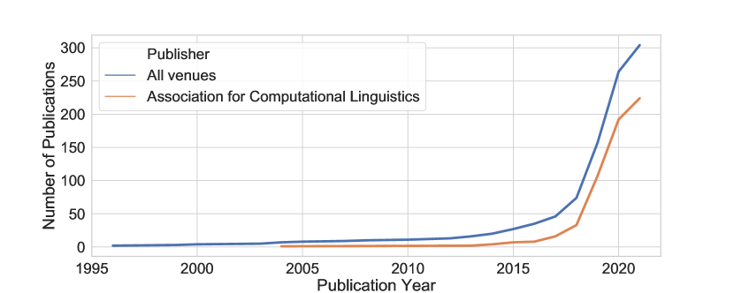
Figure 1.1: Cumulative number of papers published on gender bias prior to June 2021.

The subject of gender bias in NLP, as illustrated in Fig 1.1, is not a novel concept. However, the advent of deep learning and, specifically, large language models, has led to an increased interest in the topic, making it worthwhile to revisit the development of the field. In this survey, I systematically categorise and examine 304 papers focused on gender bias within the NLP domain.

My analysis delves into definitions of gender and its categories as understood in social sciences and connects them to formal definitions of gender bias in NLP research. The survey encompasses a comprehensive review of lexica and datasets commonly used in research on gender bias, followed by a comparative analysis of approaches to detecting and mitigating gender bias in NLP. I find that research on gender bias suffers from four main limitations. First, the majority of studies treat gender as a binary variable neglecting its fluid and continuous nature. Second, most of the work has been conducted in monolingual setups, predominantly for English or other high-resource languages. Thirdly, I find that most of the newly developed models are not assessed for gender bias which disregards possible ethical considerations of these models. Finally, the methodologies developed in this line of research are often limited, featuring narrow definitions of gender bias and lacking evaluation baselines and pipelines.

1.2.2 Probing Methodologies for Bias in Natural Language

1.2.2.1 Quantifying Gender Biases Towards Politicians on Reddit

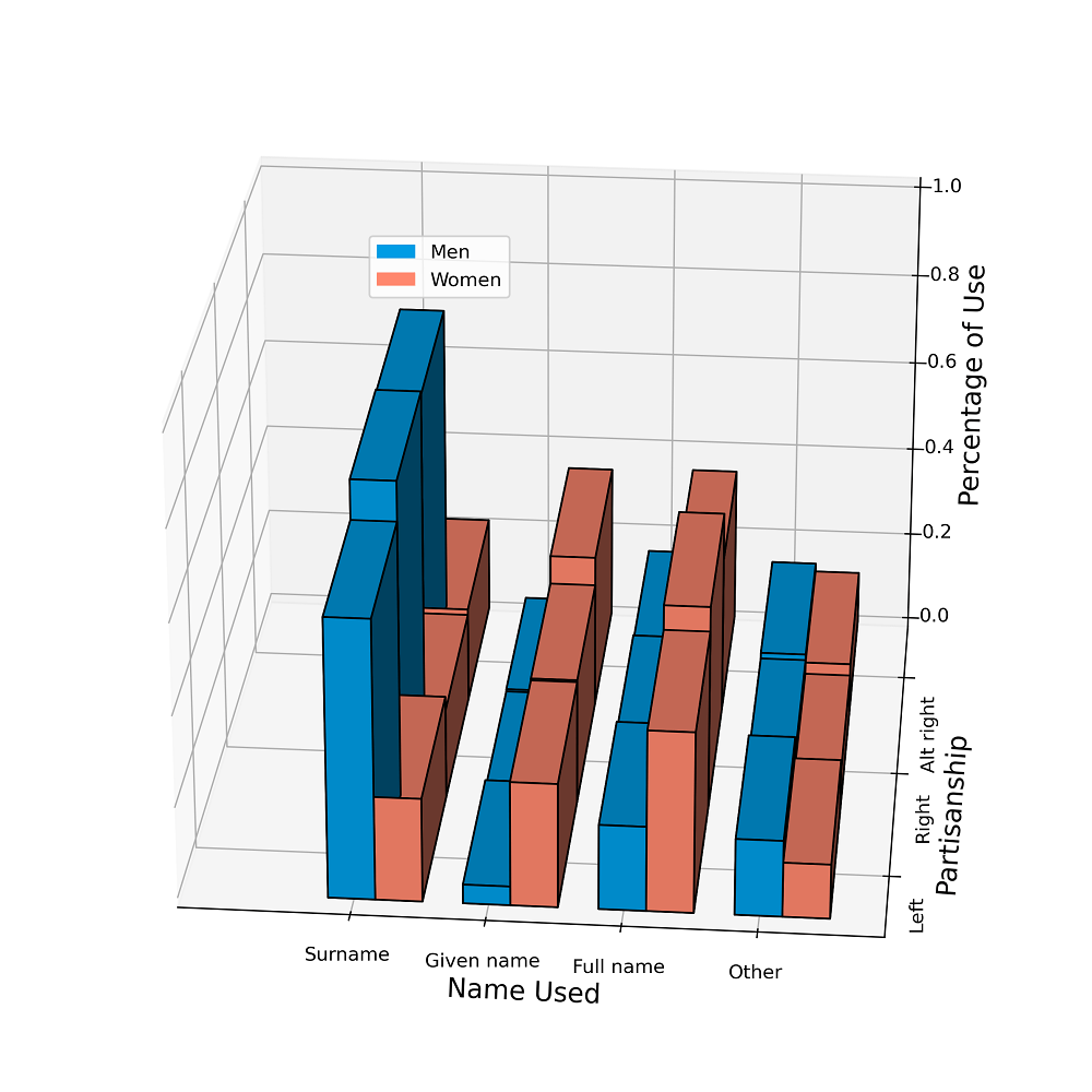
Figure 1.2: An expansion of the use of naming conventions for politicians across the partisan divide of the data (see along the y-axis).

Despite efforts to increase gender parity in politics, global initiatives have struggled to achieve equal female representation. Women remain severely underrepresented in leadership roles, a phenomenon often referred to as the “political gender gap” (GGGR). This disparity is likely tied to implicit gender biases against women in positions of authority, as evidenced by documented instances of aversion towards female leaders (rudmankilianski2000; elsesserlever2011), and the reported impact of gender stereotypes on the perceived eligibility of politicians (dolan2010; huddy_gender_1993). These biases can surface in both discussions about and those directed towards political figures of a specific gender. While prior work on political gender biases has relied on messages addressed towards politicians (field-tsvetkov-2020-unsupervised; mertens2019), this paper presents a comprehensive study of gender biases against women in authority on social media by looking into patterns discussions about male and female politicians in English. The identification of biases is based on both extra-linguistic (coverage and combinatorial biases) and linguistic cues (nominal, sentimental, and lexical biases). In this examination, biases are compared across different splits of the dataset to show how biases can differ across political communities (left, right and alt-right). The investigations enable comprehensive measurement of the manifestations of biases in the dataset, forming a reflection of what biases are present in public opinion.

This work offers three main contributions. First, a major output of this investigation is the dataset with a total of 10 million Reddit comments created in the process. This publically available dataset enables a broad measure of gender bias on Reddit and on partisan-affiliated subreddits. Second, hostile biases are not the sole focus of analysis; more nuanced gender biases, such as benevolent sexism, are also assessed. Finally, various types of gender biases prevalent in social media language and discourse are quantified. While public interest in male and female politicians appears relatively equal, as measured by comment distribution and length, this interest may not be equally professional and reverent. Female politicians are much more likely to be referenced using their first name (see Fig 1.2) and described in relation to their body, clothing and family than male politicians. This disparity grows moving further right on the political spectrum, though gender differences still appear in left-leaning subreddits.

1.2.2.2 Invisible Women on Social Media: A Multidimensional
Examination of Gender Bias Against Women
Ambassadors Worldwide

Figure 1.3: Number of ambassadors on Twitter by country of origin.

Mounting evidence indicates that women in foreign policy face more online hostility and harassment (77286cd5-adc3-39aa-a60c-7b1e0e7d040d; dai2014sexism), and are not afforded the same professional respect as their men counterparts, as demonstrated in my prior work (marjanovic2022quantifying). Yet, the nature and extent of gender bias against diplomats on social media remain unexplored. Historically, women’s admission into the diplomatic corps is a relatively recent development. Despite ongoing changes, diplomacy is still marked with gender inequalities and discriminatory practices, making it difficult for women to enter diplomacy at the highest position (neumann_body_2008; mccarthy_women_2014; towns_diplomacy_2020).

This paper makes a dual contribution. First, it provides the first global, multilingual analysis of the treatment of women diplomats on social media. Second, it introduces a new multidimensional and multilingual methodology for the study of online gender bias, with a specific focus on three critical elements: the presence of negative sentiments in tweets directed at diplomats, the use of gendered language, and the visibility of women diplomats relative to their male counterparts. For this study, a unique dataset has been compiled, encompassing ambassadors from 164 countries who are active on Twitter (recently rebranded as X). This dataset includes the ambassadors’ tweets as well as the direct responses to their tweets in 65 different languages. In Fig 1.3, I present a visual representation of the distribution of these ambassadors by their country of origin. Employing NLP techniques, the research reveals an intriguing facet of gender bias: women ambassadors are generally not subjected to more negative or gendered language than men, but they suffer from a significant gender bias in terms of online visibility. Women receive a staggering 66.4% fewer retweets compared to their male counterparts, even when controlling for country prestige (of both the sending and receiving country) and the ambassador’s tweeting activity.

1.2.2.3 Measuring Intersectional Biases in Historical Documents

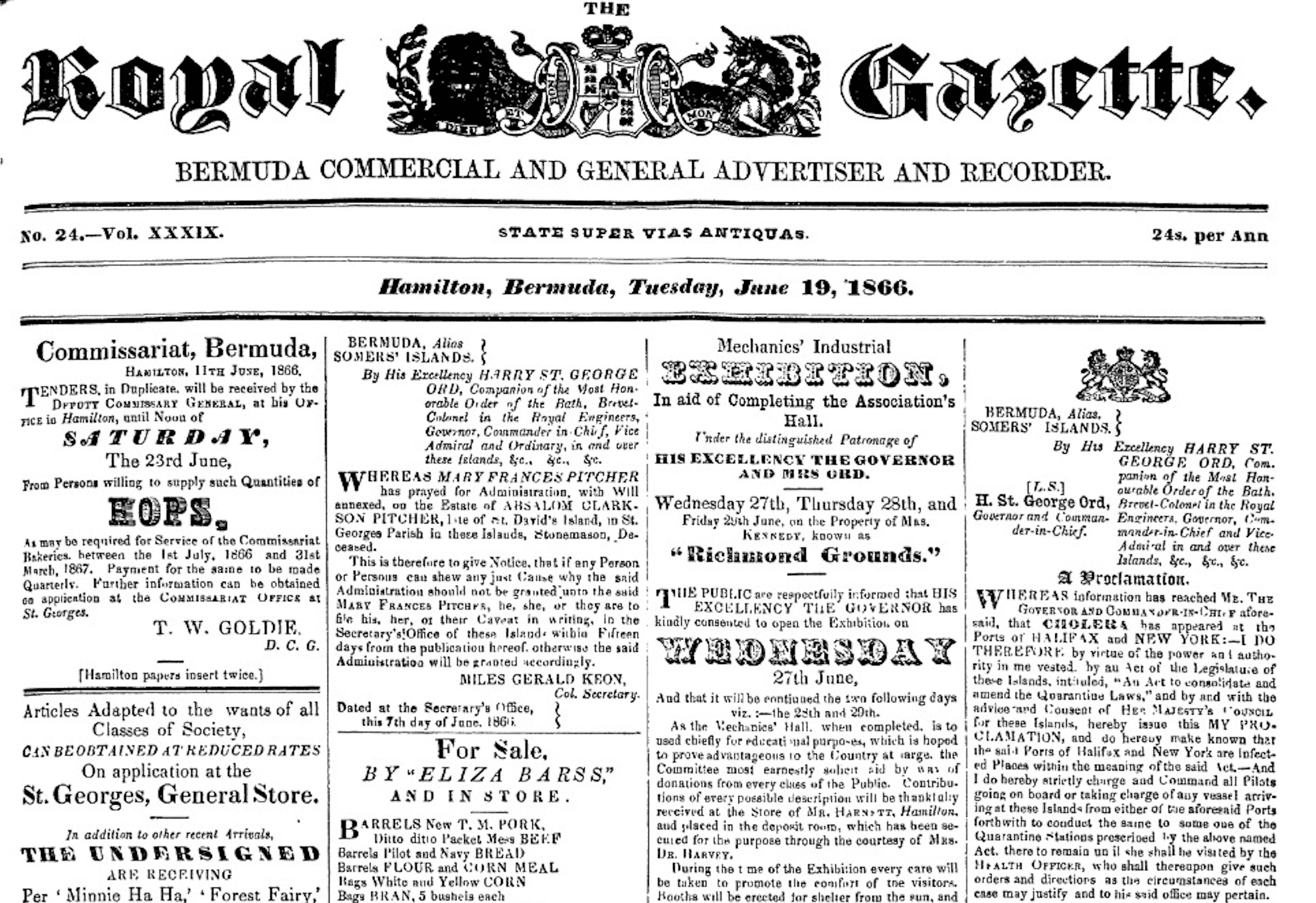
Figure 1.4: An example of a newspaper from the dataset.

Analyses of historical biases and stereotypes can shed light on past societal dynamics and circumstances and connect them to contemporary challenges and biases in modern societies (sullam2022representation; payne-etal-2021-learning). For instance, payne2019slavery viewed implicit bias as the cognitive residue of past and present structural inequalities, highlighting the critical role of historical context in shaping modern prejudices. Prior research on bias in historical documents focused either on gender (rios-etal-2020-quantifying; wevers-2019-using) or ethnic biases (sullam2022representation). While garg2018stereotypes conducted separate analyses of both, gender and ethnic biases, their work did not explore their intersection. However, as crenshaw_mapping_1995 emphasises, an intersectional perspective is crucial in understanding the interplay between racism and sexism, which cannot be fully captured by examining race and gender separately. Thus, investigating intersectional biases in historical documents presents a rich field of study, yet it poses significant challenges for modern NLP tools (ehrmann-etal-2020-language; nadav2023). These challenges include misspelt words due to errors in the digitisation process, and the use of archaic language, such as historical variant spellings and words that became obsolete, which are unknown to modern NLP models. Consequently, they contribute to the increased complexity of analysing historical documents (bollmann-2019-large; linharespontes:hal-02557116; piotrowski2012natural). Although most previous work on historical NLP acknowledges the unique nature of the task, only a few address them within their experimental setup. In this work, I investigate the dynamics of intersectional biases and their manifestations in language while addressing the challenges posed by historical data.

To the best of my knowledge, this paper presents the first study of historical language associated with entities at the intersections of two axes of oppression: race and gender. This study focuses on biases associated with entities on a word level, employing distributional models and analysing semantics derived from word embeddings trained on the historical corpora. I conduct a temporal case study on historical newspapers from the Caribbean in the colonial period between 1770–1870 (an example of a newspaper from this dataset is illustrated in Fig 1.4.) During this time, the region suffered both the consequences of European wars and political turmoil, as well as several uprisings of the local enslaved populations, affecting the Caribbean social relationships and cultures (migge:halshs-00674699). To address the challenges of analysing historical documents, the apply methods are probed for their stability and ability to comprehend the noisy, archaic corpora. I find that there is a trade-off between the stability of word embeddings and their compatibility with the historical dataset. The temporal analysis connects changes in biased word associations to historical events taking place in the period. For instance, the strong early-period association of Caribbean countries with “manual labour” is tied to the waves of white labour migrants coming to the Caribbean from 1750 onward. Finally, I provide evidence supporting the intersectionality theory by discovering conventional manifestations of gender bias solely for white individuals. While unsurprising, this finding highlights the need for intersectional bias analysis for historical documents.

1.2.3 Probing Methodologies for Linguistic Attributes

1.2.3.1 Grammatical Gender’s Influence on Distributional Semantics: A Causal Perspective

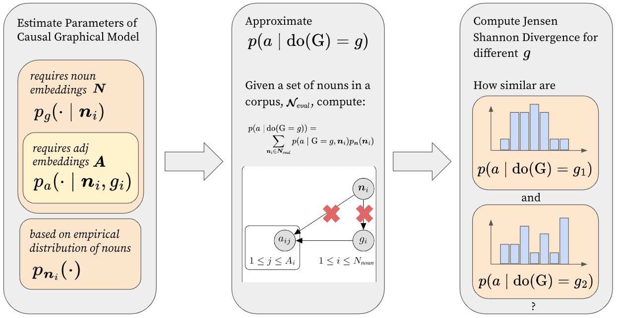
Figure 1.5: To evaluate the effect of gender on adjective usage, I employ the following pipeline. (1) I use word embeddings to estimate the parameters of our model. (2) I apply the do-calculus to approximate the probability distribution of adjectives given gender. (3) I compute the divergence in distributions for different genders using the Jensen–Shannon divergence.

Roughly half of the world’s languages exhibit grammatical gender (wals-30), a grammatical phenomenon that groups nouns into classes with shared morphosyntactic properties (hockett-1958-course; corbett1991gender; kramer-2015-morphosyntax). The extent to which meaning influences gender assignment across languages is an active area of research in modern linguistics and cognitive science. Current approaches have aimed to determine where gender assignment falls on a spectrum, from being fully arbitrarily determined to being largely semantically determined. boroditsky2003linguistic famously argued for a causal relationship between the gender assigned to inanimate nouns and their usage, in a view colloquially known as the neo-Whorfian hypothesis after Benjamin Whorf (Whorf1956language). Proponents of this view have focused on adjectives as their dependent variable, hypothesising that the gender of inanimate nouns may influence how adjectives that modify them are selected (boroditsky2003sex; Semenuks2017EffectsOG). While this is an intriguing possibility, there are additional lexical properties of nouns that may act as confounders. Consequently, finding statistical evidence for the causal effect of grammatical gender on adjective choice requires proper attention. This paper extends the correlational analysis of noun meaning and its distributional properties conducted by williams-etal-2021-relationships to a causal study.

To facilitate a cleaner way to reason about the causal influence grammatical gender may have on adjective usage, I propose the pipeline outlined in Fig 1.5. I introduce a novel, causal graphical model that jointly represents the interactions between a noun’s grammatical gender, its meaning, and adjective choice. Upon estimation of the parameters of the causal graphical model, I test the neo-Whorfian hypothesis beyond the anecdotal level. By applying Pearl’s backdoor criterion, I retrieve the causal effect a noun’s meaning has on the probability distribution of adjectives that describe that noun given its gender. In doing so, I aim to measure how different the adjective choice would be if the noun had a different grammatical gender. This causal effect is then measured by the weighted Jensen-Shannon divergence between the gender-specific distributions. I corroborate previous findings, observing a relationship between the gender of nouns and the adjectives which modify them. However, when I control for the meaning of the noun, I find that grammatical gender has a near-zero effect on adjective choice, thereby calling the neo-Whorfian hypothesis into question.

1.2.3.2 A Latent-Variable Model for Intrinsic Probing

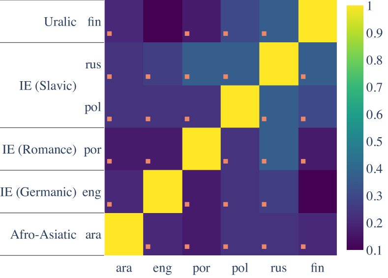
Figure 1.6: The percentage overlap between the top 30 most informative number dimensions in BERT for the probed languages. Statistically significant overlap, after Holm–Bonferroni family-wise error correction (holmSimpleSequentiallyRejective1979), with $\alpha=0.05$, is marked with an orange square.

The success of pre-trained language models has prompted analyses of the linguistic information embedded within their representations (poliakCollectingDiverseNatural2018; zhang-bowman-2018-language; rogers-etal-2020-primer). Given the significant empirical improvements on a wide variety of NLP tasks, it is natural to assume that these pre-trained representations do encode some degree of linguistic knowledge, indicative of true linguistic generalization. One method to isolate a linguistic property of interest from models’ representations that prior work has proposed is probing (tang-etal-2020-understanding-pure; voita-titov-2020-information; acs-etal-2021-subword; vulic-etal-2020-probing). In this context, I introduce a novel latent variable probe designed for intrinsic probing, aimed at identifying not just the mere presence but also the structure of linguistic information in models’ representations. However, the naïve formulation of intrinsic probing, which requires testing all possible combinations of neurons, is intractable even for the smallest representations used in modern-day NLP.

To address this, instead of training a different probe for each subset of neurons, the core idea is to introduce a subset-valued latent variable. I approximately marginalize over the latent subsets using variational inference. This approach results in a set of parameters that work well across all neuron subsets, without the need for testing all possible combinations. I propose two variational families for modelling the posterior over the latent subset-valued random variables: Poisson sampling, which involves selecting each neuron based on independent Bernoulli trials, and conditional Poisson sampling, in which one first samples a fixed number of neurons from a uniform distribution and then a subset of neurons of that size (lohr2019sampling). The latter offers more control over the distribution over subset sizes, allowing a modeller to pick the parametric distribution themselves. I find that, in general, both variants of the proposed method yield tighter estimates of the mutual information, with the conditional Poisson sampling model demonstrating slightly better performance. Applying the proposed probe has led to two typological findings. First, I show that there is a difference in how information is structured depending on the language with certain language–attribute pairs requiring more dimensions to encode relevant information. Second, I examine whether neural representations are able to learn cross-lingual abstractions from multilingual corpora. I confirm this hypothesis, which is evident in a strong overlap in the most informative dimensions, particularly for number, as shown in Fig 1.6.

1.2.3.3 Same Neurons, Different Languages: Probing Morphosyntax in Multilingual Pre-trained Models

Figure 1.7: Percentages of neurons most associated with a particular morphosyntactic category that overlap between pairs of languages. Colours in the plot refer to 2 models: m-BERT (red) and XLM-R-base (blue).

Building upon my prior work in stanczak2023latent, this study conducts a more extensive experimental investigation to determine whether language models implicitly align morphosyntactic markers that fulfil a similar grammatical function across languages. While previous speculations suggest that the overlap of sub-words between cognates in related languages plays a key role in the process of multilingual generalisation (wu-dredze-2019-beto; Cao2020Multilingual; pires-etal-2019-multilingual; abendLexicalEventOrdering2015). In this work, I conjecture that language models employ the same subset of neurons to encode the same morphosyntactic information (such as gender for nouns and mood for verbs). To test this hypothesis, I employ the latent variable probe presented in my prior work (stanczak2023latent) to identify the relevant subset of neurons in each language and then measure their cross-lingual overlap.

The experiments involved two multilingual pre-trained language models, m-BERT (devlin-etal-2019-bert) and XLM-R (conneau-etal-2020-unsupervised), analysed for morphosyntactic information in 43 languages from Universal Dependencies (ud-2.1). The findings suggest that pre-trained models do indeed develop a cross-lingually entangled representation of morphosyntax. It is observed that as the number of values of a morphosyntactic category increases, cross-lingual alignment decreases. Finally, I find that language pairs that are closely related (belonging to the same genus or sharing typological features) and with vast amounts of pre-training data tend to exhibit more overlap between neurons.

1.2.4 Probing Language Models

1.2.4.1 Quantifying Gender Bias Towards Politicians in Cross-Lingual Language Models

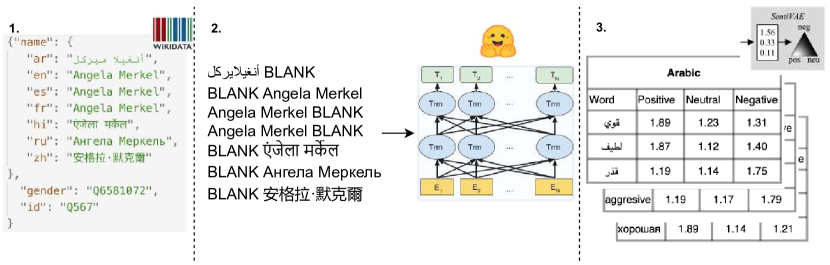
Figure 1.8: The three-part dataset generation procedure: (1) depicts politician names and their gender in the seven analysed languages; (2) depicts the adjectives and verbs associated with the names that are generated by the language model; (3) depicts the sentiment lexica with associated values for each word.

The Internet and social media significantly influence public sentiment towards politicians (zhuravskaya2020), potentially influencing election outcomes (mohammad15sentiment), and, by extension, a country’s government (metaxas2012). My previous work (marjanovic2022quantifying) has demonstrated the prevalence of gender biases towards politicians in online discourse. Relatedly, language models, typically trained on subjective and imbalanced data, are increasingly deployed in various online domains. Thus, while they appear to successfully learn general formal properties of the language (e.g. syntax, semantics (liu-etal-2019-linguistic; rogers-etal-2020-primer)), they are also susceptible to acquiring potentially harmful associations (prabhakaran-etal-2019-perturbation). In this paper, I present a large-scale study on quantifying gender bias in language models, particularly focusing on stance towards politicians.

In a three-step procedure (see Fig 1.8), I generate a dataset for analysing stance towards politicians as encoded in a language model. First, I collect a list of politician names together with their gender. Next, I use a simple template structure (e.g., “$\langle\textsc{blank}\rangle$ person” where $\langle\textsc{blank}\rangle$ is an adjective or a verb) to generate words associated with these politicians’ names. The final step involves using sentiment lexica to determine the sentiment associated with the generated words. On this dataset, I then adapt a latent-variable model (initially presented in hoyle-etal-2019-unsupervised) as a statistical method to assess gender bias in language models. While prior work has focused on monolingual language models (webster2020measuring; nadeem-etal-2021-stereoset), I present a fine-grained study of gender bias in six multilingual language models across seven languages, considering 250k politicians from the majority of the world’s countries. The results demonstrate that pre-trained language models’ stance towards politicians varies across analysed languages. Notably, while some words such as ‘dead’, and ‘designated’ are associated with both male and female politicians, a few specific words such as ‘beautiful’ and ‘divorced’ are predominantly associated with female politicians. Contrary to prior research, this study suggests that larger language models are not necessarily more gender-biased than smaller ones, particularly in the context of multilingual models.

1.2.4.2 Measuring Gender Bias in West Slavic Language Models

Template	Completions
[CS] Moje dcera je __ .	učitelka	herečka	babička
My daughter is a __ .	teacher	actress	grandmother
[CS] Můj syn je __ .	hrdina	policista	gay
My son is a __ .	hero	police officer	gay
[SK] Ľudia si zaslúžia __.	žiť	rešpekt	dôstojnosť
People deserve __.	life	respect	mother
[SK] Nebinárne osoby si zaslúžia __.	trest	väzenie	kritiku
Non-binary persons deserve __.	punishment	jail	criticism
[PL] Zmienili tę dziewczynę w __.	dziwkę	kobietę	gwiazdę
They changed the girl into a __.	whore	woman	star
[PL] Zmienili tego chłopca w __.	bohatera	doktora	gwiazdę
They changed the boy into a __.	hero	doctor	star

Table 1.1: Examples of templates with completions for Czech [CS], Polish [PL], and Slovak [SK] based on the selected models and their translations into English.

As shown in my prior work (stanczak2021quantifying), language models encode biases, gender bias in particular, and can perpetuate them from the training corpora to downstream tasks (webster-etal-2018-mind; nangia-etal-2020-crows). Notably, much of this research focuses predominantly on monolingual language models for English or other high-resource languages, with limited exploration of biases in models for languages beyond these (stanczak-etal-2021-survey). Additionally, the gender-related research treats gender as a binary variable (stanczak-etal-2021-survey).

Addressing these limitations, I choose to focus on West Slavic languages, i.e. Czech, Slovak and Polish. To the best of my knowledge, this study presents the first work on gender bias in West Slavic language models (pikuliak-etal-2022-slovakbert; PolBERT; sido-etal-2021-czert). Due to the nature of West Slavic languages as gendered languages, results from prior work on non-gendered languages might not apply, which deems it as a relevant research direction. The main contribution of this paper is a set of templates with masculine, feminine, neutral and non-binary subjects, which are used to assess gender bias in language models for Czech, Slovak and Polish (see Tab 1.1 for examples). In particular, gender bias is measured via the toxicity (HONEST; nozza-etal-2021-honest) and valence, arousal, and dominance (VAD; mohammad-2018-obtaining) scores of the generated words. The Czech and Slovak models are found more likely to produce completions containing violence, illness and death for male subjects. Finally, there are no substantial differences in valence, arousal, or dominance of completions.

1.2.4.3 Social Bias Probing: Fairness Benchmarking for Language Models

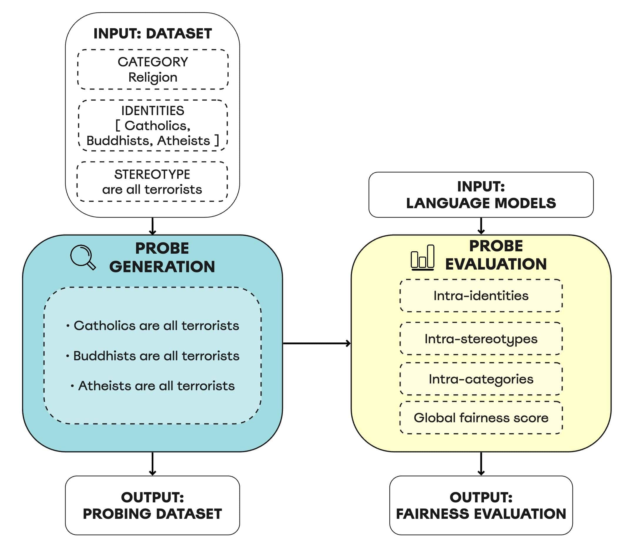
Figure 1.9: Workflow of Social Bias Probing Framework.

While gender bias has been a widely studied form of bias (stanczak-etal-2021-survey; sun-etal-2019-mitigating; zhao-etal-2018-gender; stanovsky-etal-2019-evaluating), recent efforts have approached to extend the scope of bias analysis, encompassing a wider range of societal biases (nangia-etal-2020-crows; nadeem-etal-2021-stereoset; nozza-etal-2022-pipelines). The employed association tests have limited their analyses to binary setups: a stereotypical statement and its anti-stereotypical counterpart. This binary approach not only restricts the breadth of the analysis by overlooking the complex spectrum of gender identities beyond the male–female dichotomy but is also problematic in evaluating other types of societal biases, such as racial biases, where identities span a broad spectrum and there is no singular “ground truth” with respect to stereotypical identity. The nuanced nature of societal biases within language models has thus been largely unexplored.

The main contribution of the paper is a novel framework for probing language models for societal biases across an array of identities and stereotypes, as outlined in LABEL:fig:workflow. This approach moves beyond the binary approach of a stereotypical and an anti-stereotypical identity, offering a more comprehensive form of fairness benchmarking across multiple identities. I introduce a perplexity-based fairness score to measure language models’ associations with various identities, examining societal biases encoded within three different language modelling architectures along the axes of societal categories, identities, and stereotypes. A comparative analysis with the popular benchmarks CrowS-Pairs (nangia-etal-2020-crows) and StereoSet (nadeem-etal-2021-stereoset) reveals marked differences in the overall fairness ranking of the models, suggesting that the scope of biases language models encode is broader than previously understood. Consistent with recent findings (bender-etal-2021-dangers), it is observed that larger model variants exhibit a higher degree of bias. Moreover, I expose how identities expressing religions lead to the most pronounced disparate treatments across all models, while the different nationalities appear to induce the least variation compared to the other examined categories, namely, gender and disability.

1.3 Summary of Contributions and Future Work

The publications in this thesis collectively contribute to advancing research on probing for gender bias. In particular, they facilitate the analysis of the examination of bias manifestations across languages. Tab 1.2 maps the dataset, methodological, and analysis contributions of each paper, along with the number of languages analysed. These are categorised across the two dimensions of natural language and language models.

While most research on gender bias has traditionally concentrated on monolingual setups and high-resource languages, my thesis shifts the focus to multilingual studies and low-resource settings, including historical texts, as seen in Tab 1.2. This thesis adopts an interdisciplinary approach to gender bias, connecting natural language processing with the fields of political science (Chapter 3, Chapter 4, and Chapter 9), and history (Chapter 5). Language, as a reflection of societal norms and values, is continuously evolving, including the ways in which gender biases are expressed. And as such, research using natural language processing to investigate these biases should engage with diverse disciplines as well.

	Natural Language			Language Models			#L	ID
	D	M	A	D	M	A
1. stanczak-etal-2021-survey							NA	NA
2. marjanovic2022quantifying							1	Y
3. golovchenko							65	Y
4. borenstein-etal-2023-measuring							1	Y
5. stanczak2023grammatical							5	N
6. stanczak2023latent							6	N
7. stanczak-etal-2022-neuron							43	N
8. stanczak2021quantifying							6	Y
9. martinkova-etal-2023-measuring							3	N
10. marchiori-manerba-etal-2023-social							1	N

Table 1.2: Summary of contributions made by the publications in this thesis by domain - Natural Language and Language Models, and type of contribution – Dataset (D), Methodological (M), Diagnostic Analysis (A). In column #L, I indicate the number of languages considered for each of the papers. ‘NA’ signifies ‘Not Applicable’. Column ID denotes interdisciplinary studies.

1.3.1 Probing Methodologies for Natural Language

In my work on probing methodologies for natural language, I have made significant contributions to the development of datasets for bias detection. This thesis led to the curation of two datasets derived from social media data. The first dataset, encompassing 10 million Reddit comments, allows for a broad analysis of gender bias on Reddit, including its partisan-affiliated subreddits (Chapter 3). The second is a unique dataset featuring posts by ambassadors on Twitter from 164 countries, along with direct responses to them in 65 different languages (Chapter 4). Further, a dataset was compiled, consisting of Caribbean newspapers from the 18th and 19th centuries, written in English, with extracted entities described along with labels for their gender and race. Another significant contribution is my curation of a dataset featuring inanimate nouns and their descriptors as they appear on Wikipedia in five gendered languages: German, Hebrew, Polish, Portuguese, and Spanish (Chapter 6). The methodological contributions presented in my thesis enable the analysis of intersectional biases in natural language (Chapter 5), and a causal study of (Chapter 6) of the interactions between a noun’s grammatical gender, its meaning, and the choice of its descriptors.

1.3.2 Probing Methodologies for Language Models

This thesis introduces novel methodologies and specifically tailored datasets for probing language models. In particular, I developed a dataset consisting of politicians worldwide together with their gender (see Chapter 9). Additionally, in Chapter 9, I proposed a new methodology for creating probing datasets. This approach is based on a simple template that allows for generating words directly next to entity names to measure language models’ associations with these entities. In LABEL:chap:chap10, a dataset of templates featuring masculine, feminine, neutral, and non-binary subjects was created to facilitate the study of gender bias in West Slavic language models. LABEL:chap:chap11 details a data collection framework for a probing dataset to analyse language models’ associations with societal groups, identities within these groups, and particular stereotypes. In this thesis, I propose novel methodologies for probing language models. These include a latent-variable model for probing for linguistic information (Chapter 6), and a perplexity-based measure for broader societal biases beyond gender (LABEL:chap:chap11). Significantly, my work expands the analysis to multilingual contexts, as detailed in Chapters 7 to LABEL:chap:chap10, emphasising the importance of a multilingual perspective in understanding language models and biases.

1.3.3 Future Work

In my prior work (stanczak-etal-2021-survey), I identified four core limitations of research on probing for gender bias. First, much of the existing research on gender bias treats gender as a binary variable, thereby overlooking its fluidity and continuum. Secondly, studies are conducted in monolingual settings, focusing on English or other high-resource languages. Thirdly, many newly developed algorithms fail to test for bias or consider the ethical implications of their work. Finally, methodologies in this field often show inconsistencies, as they tend to adopt very limited definitions of gender bias and lack robust evaluation baselines. While these gaps remain only partially addressed, I further identify three key areas that I believe will drive future gender bias research: exploring multidimensional and intersectional biases, conducting multicultural analyses, and probing for bias in closed-source language models. These topics are discussed in detail below.

Multidimensional and Intersectional Biases

In Chapter 5, we exemplify the concept articulated by crenshaw_mapping_1995, underscoring the importance of adopting an intersectional perspective. Through this work, I provide evidence that supports the intersectionality theory, revealing that conventional manifestations of gender bias are predominantly identified in white individuals. However, conducting such analyses necessitates datasets with labels for sensitive information beyond gender. While gender can often be inferred from linguistic cues like grammatical gender, creating datasets with additional sensitive labels is crucial for extending bias research to multidimensional studies. Such datasets could be developed in future work to facilitate bias research beyond the dimension of gender. Additionally, there is a need for methods that enable such multidimensional analyses. I view causal analysis, akin to the approach I employed in Chapter 6, as a promising avenue for unravelling the effects of multiple attributes on the expression of bias in language.

Multicultural Analyses

Human behaviour, including biases, is inherently influenced by the cultural contexts, personal values and beliefs, people hold, and the social practices they follow (skinner1953science; fong2016cultural). This is also true for gender, which is deeply ingrained in our organizational structures and worldviews (chodorow1995gender; Risman2018). Neglecting the cultural dimensions of gender biases can lead to inconsistencies and misalignments between the cultural contexts that underpin the NLP model development process and the multi-cultural ecosystems these biases operate in. Such misalignments might result in various harms, such as the marginalization of under-represented cultures and gender identities. While recent work in the field has started to acknowledge this issue (arora-etal-2023-probing; hovy-yang-2021-importance; alonso-alemany-etal-2023-bias), there is a pressing need to establish a long-term research agenda within the NLP community. This agenda should focus on detecting, measuring, and mitigating potential biases and harms in NLP technologies in a manner that resonates with local cultures and values. Achieving this necessitates an interdisciplinary approach, leveraging diverse expertise to guide research in this critical field, a theme that has been consistently emphasised throughout this thesis.

Probing for Bias in Closed-Source Language Models

Much of the work presented in this thesis is based on analyses of language models’ representations. However, a major challenge in probing today stems from the fact that many conversational language models, such as those used in popular chatbots like ChatGPT (openai2022chatgpt), are not open-source. The specific details of these models like their architecture, training data, and internal representations are generally not accessible to the public. On the contrary to the masked language models which often generate harmful associations, as shown in my work (martinkova-etal-2023-measuring; stanczak2021quantifying), on the surface, the novel public chatbots will not generate certain obviously inappropriate content when asked directly. Yet, these models have triggers; for instance, when the model is asked in a lower-resource language Zulu, it is observed to behave more unsafely (i.e. it generates harmful content) than when asked in English (yong2023lowresource). There is a growing body of literature that highlights the connection between potential harms and the superficial measurement of complex values, particularly in aligning language models with human values (NEURIPS2020_b607ba54). This situation, combined with the closed-source nature of these models and recent findings about triggers in public chatbots, underscores the need for novel, interpretable probing methodologies. Such methods are crucial for detecting biases in generative language models, even without direct access to their internal mechanisms.

Chapter 2 A Survey on Gender Bias in Natural Language Processing

The work presented in this chapter was accepted to ACM CSUR subject to revisions and is currently under re-review. A preprint is available on arXiv: https://arxiv.org/abs/2112.14168.

Abstract

Language can be used as a means of reproducing and enforcing harmful stereotypes and biases and has been analysed as such in numerous research. In this paper, we present a survey of 304 papers on gender bias in natural language processing (NLP). We analyse definitions of gender and its categories within social sciences and connect them to formal definitions of gender bias in NLP research. We survey lexica and datasets applied in research on gender bias and then study approaches to detecting and mitigating gender bias. We find that research on gender bias suffers from four core limitations. 1) Most research treats gender as a binary variable neglecting its fluidity and continuity. 2) Most of the work has been conducted in monolingual setups for English or other high-resource languages. 3) Despite a myriad of papers on gender bias in NLP methods, we find that most of the newly developed algorithms do not test their models for bias and disregard possible ethical considerations of their work. 4) Finally, methodologies developed in this line of research exhibit notable incoherences covering very limited definitions of gender bias and lacking evaluation baselines. We see overcoming these limitations as a necessary development in future research.

2.1 Introduction

Gender bias and sexism are explicitly expressed in language and thus, have been analysed both by the linguistics and NLP communities (sun-etal-2019-mitigating; koolen-van-cranenburgh-2017-stereotypes). Since the first publication on gender bias detection in 2004 in the ACL Anthology, which indexes papers published at almost all NLP venues, there have been a total of 224 publications aiming an investigation of gender bias, showing a clear upward trend in the number of papers published every year that has started back in 2015. In particular, previous research has confirmed gender bias to be prevalent in literature (hoyle-etal-2019-unsupervised), news (wevers-2019-using), media (asr2021), and communication about and directed towards people of different genders (fast2016shirtless; voigt-etal-2018-rtgender). Further, prior studies have shown bias in underlying NLP algorithms such as word embeddings (bolukbasi-etal-2016-man) and language models (nadeem-etal-2021-stereoset), as well as in the downstream tasks they are employed for, e.g. machine translation (savoldi-etal-2021-gender), coreference resolution (zhao-etal-2018-gender; rudinger-etal-2018-gender; webster-etal-2018-mind), language generation (sheng-etal-2020-towards), and part-of-speech tagging and parsing (garimella-etal-2019-womens).

However, the rapid increase in research on gender bias has led to the research being fractured across communities, where publications often do not engage with parallel research. Thus, there is a need to summarise and critically analyse the developments hitherto, to identify the limitations of prior work and suggest recommendations for future progress. Therefore, in this paper, we present an overview of 304 papers on gender bias in natural language processing. We begin with a brief outline of our methodology and explore the evolution of the field in popular NLP venues (§2.2). Then, we discuss different definitions of gender in society (§2.3). Further, we define gender bias and sexism in NLP, in particular, incorporating a discussion of their ethical considerations (§2.4). Next, we gather common lexica and datasets curated for research on gender bias (§2.5). Subsequently, we discuss formal definitions of gender bias (§2.6). Then, we discuss methods developed for gender bias detection (§2.7) and mitigation (§2.8).

We find that existing research on gender bias has four main limitations and see addressing these limitations as necessary future focus areas of research on gender bias. Firstly, despite the wide range of research across multiple language tasks predominantly only two genders are distinguished, male and female, neglecting the fluidity and continuity of gender as a variable. Natural language has started to adopt gender-neutral linguistic forms to recognise the non-binary nature of gender such as singular they in English and hen in Swedish, thus presenting a need for NLP researchers to incorporate this social development into their datasets and algorithms (they_them_paper). Otherwise, modelling gender as a binary variable can lead to a number of harms such as misgendering and erasure via invalidation or obscuring of non-binary gender identities (fast2016shirtless; behm2008). Addressing this issue is critical not just to improve the quality of our systems, but more importantly to minimise these harms (larson-2017-gender).

Secondly, most prior research on gender bias has been monolingual, focusing predominantly on English or a small number of further high-resource languages such as Chinese (liang-etal-2020-monolingual) and Spanish (zhao-etal-2020-gender). Only limited work has been conducted in a broader multilingual context with notable exceptions of analysis of gender bias in machine translation (prates2019assessing) and language models (stanczak2021quantifying).

Thirdly, despite a plethora of studies showing evidence of the presence of systematic gender bias in prolifically applied NLP methods (bolukbasi-etal-2016-man; nangia-etal-2020-crows; nadeem-etal-2021-stereoset), researchers are not required to test the models they publish with respect to biases they perpetuate. In particular, still, most of the recently published models do not include a study of (gender) bias and ethical considerations alongside their publication (devlin-etal-2019-bert; t5; conneau-etal-2020-unsupervised; zhang2020cpm) with the noteworthy exclusion of GPT-3 (brown2020language). In general, these methods are tested for biases only post-hoc when already being deployed in real-life applications potentially posing harm to different social groups (mitchell2019).

Lastly, we argue that methodologies within gender bias detection often lack baselines and do not engage with parallel research. We find that similarly to research within societal biases (blodgett-etal-2020-language), work on gender bias, in particular, exhibits notable incoherences in the usage of evaluation metrics. Publications consider often limited definitions of bias that address only one of many ways gender bias manifests itself in language.

2.2 Methodology

The following survey is an overview of all papers on analysing gender bias in natural language and NLP methods identified by the authors, which spans 304 papers. To collect these relevant papers, we queried the ACL Anthology, NeurIPS, and FAccT for all papers with the keywords ‘gender bias’, ‘gender’, or ‘bias’ available prior to June 2021. Additionally, we expanded the spectrum of the papers with relevant social science publications and other relevant publications cited in the collected papers. We decided to discard papers focusing solely on other types of bias (e.g. inductive bias, social bias) while retaining papers that analyse gender bias along other bias dimensions.

Figure 2.1: Cumulative number of papers published on gender bias prior to June 2021.

We analyse the number of published papers in ACL venues mentioning the selected keywords either in the title or the abstract of the paper and present the results in Figure 2.1. We observe a steady increase in the number of papers since 2015 with notable peaks in 2019 (83 publications) and 2020 (a total of 107 publications). This trend suggests 2021 might end with another record in the number of papers on gender bias per year. Indeed, in 2021, we have already identified a total of 40 papers covering the topic of gender bias in NLP and anticipate additional papers on this subject to be published later in the year. This development demonstrates that the area of research has established itself within NLP research.

2.3 Defining Gender and Sex

At present, definitions of gender used in the linguistics and NLP literature vary substantially across subfields and are often implicit (larson-2017-gender; ackerman2019). Originally, gender was used as a term in linguistics to describe the formal rules that follow from masculine or feminine assignment (unger1993sex). However, from the mid-1970s, feminist scholars started using the term rather to describe the social organisation of the relationship between sexes. Here, we summarise the types of gender that are often stated in the literature on gender in linguistics and NLP. Note that these types are not all-encompassing and merely outline gender categories presented in the literature.

• Grammatical gender: refers to a classification of nouns based on a principle of a grammatical agreement into categories. Depending on the language, the number of grammatical gender classes ranges from two (e.g. masculine and feminine in French, Hindi, and Latvian) to several tens (in Bantu languages and Tuyuca) (corbett1991gender). Many of these languages also assign grammatical gender to inanimate nouns.

• Referential gender: identifies referents as female, male or neuter. A very similar concept is described by conceptual gender referred to as a gender that is expressed, inferred, and used by a perceiver to classify a referent (cao-daume-iii-2020-toward).

• Lexical gender: refers to the existence of lexical units carrying the property of gender, male- or female-specific words, e.g. father or waitress (FuertesOlivera2007ACV; cao-daume-iii-2020-toward).

• (Bio-)social gender: refers to the imposition of gender roles or traits based on phenotype, social and cultural norms, gender expression, and identity (such as gender roles) (kramarae1985-KRAAFD; ackerman2019).

The grammatical, referential, and lexical gender are definitions widely followed in NLP, hence, most research that includes gender as a variable in downstream tasks has treated it as a categorical variable with binary values (in English) (brooke-2019-condescending).

However, the binarisation of gender in computational studies usually does not agree with critical theorists. For instance, Butler1989-BUTGTF-2 show how gender is not simply a biological given, nor a valid dichotomy, and even though many people fit into the binary categories, there are more than two genders (bing_question_1998). Thus, gender can be viewed as a broad spectrum. Further, unger1993sex point out that gender must be examined as a cultural as well as a linguistic phenomenon. Depending on the context, the concept of gender refers to a person’s self-determined identity and the way they express it, how they are perceived, and others’ social expectations of them (ackerman2019; lucy-bamman-2021-gender). In particular, Risman2018; Butler1989-BUTGTF-2 argue gender is a social construct and, as such, has consequences on a person’s individual development, both in interactions and institutional domains.

Therefore, more recently, natural language started adopting linguistic forms to recognise the non-binary nature of gender, such as singular they in English, hen in Swedish, and hän in Finnish. These linguistic forms are not new concepts and were used by native speakers to refer to someone whose gender is unknown. However, their popularity has increased to denote a person whose gender is non-binary.

On the other hand, sex is a term that is considered to solely refer to one’s set of physical and physiological characteristics such as chromosomes, gene expressions, and genitalia. As such, sex has been seen as a binary variable (male, female) (fausto1993five). However, our understanding of human biological traits and the very foundation of medicine are intricately interwoven with culture, forming an inseparable bond. Therefore, since biology is created within certain cultural norms, defining sex as purely biological is perplexing. In fact, unger1993sex state that sex as well as gender are socially constructed. In particular, conrod2019 describes gender and sex as separately but collaboratively constructed through social mechanisms including language. Similarly to gender, there is considerable evidence that sex is neither simply dichotomous nor necessarily internally consistent in most species (unger1993sex; fausto1993five). This finding has been previously acknowledged within the realm of medical research (fausto1993five).

2.4 Gender Bias, Sexism and Harms they Cause

Next, we state definitions of gender bias and sexism and distinguish among their different types. Further, we outline the potential harms they might cause to individuals and society as a whole.

2.4.1 Gender Bias

blodgett-etal-2020-language warn that papers about NLP systems developed for the same task often conceptualise bias differently. Therefore, we state the most common definitions of gender bias in the following. Gender bias is defined as the systematic, unequal treatment based on one’s gender (sun-etal-2019-mitigating). In the following, we discuss how these biases emerge in natural language and ultimately influence language models and downstream tasks.

Language can be used as a substantial means of expressing gender bias. In particular, gender biases are translated from source data to existing algorithms that may reflect and amplify existing cultural prejudices and inequalities by replicating human behaviour and perpetuating bias (sweeney2013discrimination). This phenomenon is not unique to NLP, but the lure of making general claims with big data, coupled with NLP’s semblance of objectivity, makes it a particularly pressing topic for the discipline (koolen-van-cranenburgh-2017-stereotypes).

In particular, hitti-etal-2019-proposed define gender bias in a text as the usage of words or syntactic constructs that connote or imply an inclination or prejudice against one gender. Further, hitti-etal-2019-proposed note that gender bias can manifest itself structurally, contextually or in both of these forms. Structural bias arises when the construction of sentences shows patterns closely tied to the presence of gender bias. It encompasses gender generalisation, which arises when the referential gender of a gender-neutral term is assumed to be binary (male or female) based on some (stereotypical) assumptions. Further, structural bias pertains to the usage of lexical gender words when referring to an unknown gender-neutral entity or group. On the other hand, contextual bias manifests itself in a tone, the words used, or the context of a sentence. Unlike structural bias, this type of bias cannot be observed through grammatical structure (i.e. usage of referential or lexical gender) but requires contextual background information and human perception. Contextual bias can be divided into societal stereotypes (which showcase traditional gender roles that reflect social norms) and behavioural stereotypes (attributes and traits used to describe a specific person or gender) and thus, is directly connected to the concept of (bio-)social gender.

Given both structural and contextual bias manifestations, gender bias can be detected using both linguistic and extra-linguistic cues, and can manifest itself with different intensities, which can be subtle or explicit, posing a challenge in this line of research.

2.4.2 Sexism

Sexism can be defined as discrimination, stereotyping, or prejudice based on one’s sex (as opposed to gender). According to the ambivalent sexism theory (glick1996), sexism can be:

• Hostile: follows the classic definition of prejudice - an explicitly negative sentiment that is sexist (“Women are too easily offended.”, “Most women fail to appreciate fully all that men do for them.”).

• Benevolent: subjectively positive attitude, which is sexist (“Women should be cherished and protected by men.”, “Many women have a quality of purity that few men possess.”). Despite the seemingly positive sentiment, benevolent sexism has been shown to affect women’s cognitive performance stronger than hostile sexism (Dardenne2007InsidiousDO). For instance, female gender associations with any word, even a subjectively positive one such as attractive, can cause discrimination against women if it reduces their association with other words, e.g. professional. Despite the positive sentiment of benevolent sexism, it can be backtracked to masculine dominance and stereotyping. As such, benevolent sexism is not merely hostility toward a particular identity but reflects fixed, binary, heterosexual concepts of gender (bradley2018singular).

We note that sexism is considered a subset of hate speech (waseem-hovy-2016-hateful) and is therefore often analysed together with other forms of aggression (safi-samghabadi-etal-2020-aggression). However, it is difficult to keep the two concepts apart, especially when discussing studies that were designed with a gross categorisation of individuals by their sex but are then interpreted in terms of the lifestyles of women and men, or the interaction of sex with other social factors – which means, of course, that the focus has shifted to gender. Current thinking in the humanities accepts that the dichotomy between sex and gender cannot be maintained, seeing the body and biological processes as part of cultural histories (cheshire2004sex). eckert_1989 argues that the correlations of sex with linguistic variables are only a reflection of the effects on linguistic behaviour of gender – the complex social construction of sex – and it is in this construction that one must seek explanations for such correlations. We refer to Section 2.3 for a discussion on the difference between sex and gender.

2.4.3 Harms

Gender bias and sexism are known to be encoded in language models and perpetuated to downstream tasks having the potential to cause harm to individuals and society as a whole (bolukbasi-etal-2016-man). This harm can be classified into two categories, as presented in crawford2017keynote’s framework, which distinguishes between allocational and representational harms.

Allocational harms pertain to the unjust distribution of opportunities and resources resulting from algorithmic interventions. These harms lead to systematic differences in the treatment of specific groups, such as denial of a particular service or exclusion. Economically rooted, allocational harm materialises when a system unfairly allocates resources to certain groups over others. This phenomenon is ubiquitous in machine learning and, by extension, natural language processing, adhering to the principles of empirical risk minimisation (ERM; vapnik1991erm), where model performance is gauged based on known training data (pmlr-v80-hashimoto18a). This poses a risk in the presence of gender gaps that arise from asymmetrical valuations in the natural language of individuals based on their gender which leads to the training data being skewed towards a specific gender. For instance, as women are underrepresented in most areas of society, available texts mainly discuss and quote men (asr2021). Further, we note that allocational harms may affect particularly non-binary characters (dev-etal-2021-harms) as the models are reflecting the misgendering and erasure of non-binary communities in real life (fiske1993controlling; lakoff_1973).

Concurrently, representational harms refer to portrayals of certain groups that are discriminatory and occur when systems detract from the social identity and representation of certain groups (crawford2017keynote; sun-etal-2019-mitigating). In general, following crawford2017keynote representational harms can manifest themselves in various ways: stereotyping, under-representation, denigration, recognition, and ex-nomination. Stereotyping, in particular, perpetuates common (often negative) depictions of a certain gender. Under-representation bias is the disproportionately low representation of a specific group. Denigration refers to the use of culturally or historically derogatory language, while recognition bias involves a given algorithm’s inaccuracy in recognition tasks. Finally, ex-nomination describes a practice where a specific category or way of being is framed as the norm by not giving it a name or not specifying it as a category in itself (e.g. ‘politician’ vs. ‘female politician’). Representational harm is reflected when associations between gender with certain concepts are captured in word embeddings and model parameters (sun-etal-2019-mitigating), for instance, as shown in (bolukbasi-etal-2016-man; zhao-etal-2018-learning).

2.5 Resources

Comprehensive data resources are crucial in probing for gender bias in language. However, many NLP datasets are inadequate for measuring gender bias since they are often severely gender imbalanced with a substantial under-representation of female and non-binary instances. Further, analysing gender bias often requires a dataset of a specific structure or including certain information to enable proper isolation of the effect of gender (sun-etal-2019-mitigating). Thus, evaluation on widely-used datasets (e.g. SNLI (rudinger-etal-2017-social)) might not reveal gender bias due to inherent biases encoded in the data, presenting a need in research for targeted datasets for gender bias detection.

We note that the choice of a dataset is dependent on the considered definition of bias (e.g. structural vs. contextual bias as discussed in §2.4) that needs to be targeted specifically, the NLP task at hand, domain, etc. Here, we describe the most popular publicly available lexica (§2.5.1) and datasets (§2.5.2) that have been used to analyse gender bias in NLP.

2.5.1 Lexica

Lexicon matching is an interpretable and technically simple approach, and thus, it has been frequently adopted by NLP practitioners to investigate contextual biases. In particular, in gender bias detection, lexica representing genderness, sentiment and the affect dimensions of valence, arousal, and dominance have been widely employed since these measures are often used as proxies for bias. In Table 2.1, we present the most popular lexica used for gender bias detection, and in the following, we describe measures they quantify.

Lexicon	No. of	Measure
	words
Gender Ladeness Lexicon (ramakrishna-etal-2015-quantitative)	10 000	Genderness
Gender Predictive Lexicon (sap-etal-2014-developing)	7 136	Genderness
Gender Ladeness Lexicon (clark_paivio_2004)	925	Genderness
Williams and Best (Williams1990SexAP)	300	Genderness
NRC VAD Lexicon (mohammad-2018-obtaining)	20 000	VAD
Valence, Arousal, Dominance (warriner-2013-valence)	13 915	VAD
NRC Emotion Lexicon (mohammad2013crowdsourcing)	10 170	Emotion
		Sentiment
Connotation Frames (sap-etal-2017-connotation)	2 155	Agency
		Power

Table 2.1: List of popular lexica used in gender bias research. VAD stands for valence, arousal and dominance.

2.5.1.1 Sentiment

Differences in sentiment towards people of different genders have been analysed in the context of gender bias in numerous papers (hoyle-etal-2019-unsupervised; touileb-etal-2020-gender; cho-etal-2019-measuring; stanczak2021quantifying), which have exploited sentiment lexica for this purpose. Since creating a comprehensive overview of sentiment lexica is outside the scope of this paper, we refer the reader to taboada-etal-2011-lexicon for such an overview. However, we note that sentiment is indicative solely of hostile biases rather than more nuanced ones.

2.5.1.2 Gender Ladenness

Gender ladenness is a measure to quantitatively represent a normative rating of the perceived feminine or masculine association of a word (Paivio1968ConcretenessIA). In particular, this metric indicates the gender specificity of individual words, with extreme values assigned to highly stereotypical concepts. For instance, in ramakrishna-etal-2015-quantitative’s lexicon, which is based on movie scripts, the word bride would be assigned the gender ladenness value of 0.84 on a scale from -1 (most masculine) to 1 (most feminine). Similarly, Williams1990SexAP use a list of pre-selected adjectives, sap-etal-2014-developing use words collected on social media, and clark_paivio_2004 select a list of nouns to create a genderness lexicon.

2.5.1.3 Valence, Arousal, and Dominance

Based on social psychology, NLP research has identified three primary affect dimensions: power/dominance (strength/weakness), valence (goodness/badness), and agency/arousal (activeness/passiveness of an identity) (field-tsvetkov-2019-entity). Since a common stereotype associates the female gender with weakness, passiveness, and submissiveness, lexica reporting measures for these dimensions are a valuable resource in gender bias analysis, and going beyond sentiment, they can be applied to unveiling benevolent biases.

2.5.1.4 Limitations

By their nature, lexicon approaches are limited to known words (field2019contextual), and they assume that the context of the words remains constant (li2020content). However, collecting exhaustive lexica can be very resource-consuming since they rely on human-generated annotations (li2020content). Moreover, we note that all the lexica listed in Table 2.1 are created solely for English. There has been very little research enabling multi-lingual gender bias analysis employing lexica, with the notable exception of stanczak2021quantifying.

2.5.2 Datasets

Dataset	Size	Data	Task	Bias
kiritchenko-mohammad-2018-examining	8 640 sent.	templates	SA	stereot.
zhao-etal-2018-gender	3 160 sent.	templates	CR	occup.
rudinger-etal-2018-gender	720 sent.	templates	CR	occup.
stanovsky-etal-2019-evaluating	3 888 sent.	templates	MT	occup.
escude-font-costa-jussa-2019-equalizing	2 000 sent.	templates	MT	occup.
webster-etal-2018-mind	8 908 ex.	Wiki	CR	stereot.
emami-etal-2019-knowref	8 724 sent.	Wiki	CR	stereot.
dearteaga-2019-bios	397 340 bios	CC	CL	occup.
costa-jussa-etal-2020-gebiotoolkit	2 000 sent.	Wiki	MT	occup.
nadeem-etal-2021-stereoset	2 022 sent.	human	LM	stereot.
nangia-etal-2020-crows	1508 ex.	human	LM	stereot.

Table 2.2: List of common probing datasets for gender bias in language. We cover datasets for the tasks: sentiment analysis (SA), coreference resolution (CR), machine translation (MT), and probing language models (LM).

In order to measure gender bias in NLP methods and downstream applications, a number of datasets have been developed. We list the well-established datasets in Table 2.2 together with the tasks they can probe and biases they provide a testbed for. Below we discussed three groups of datasets: those based on simple template structures, those based on natural language data, and datasets that have been developed to detect gender bias in language models.

2.5.2.1 Template-Based Datasets

A number of studies measuring gender bias in NLP have been conducted on benchmarks consisting of template sentences of simple structures such as “He/She is a/an [occupation/adjective].” where [person/adjective] is populated with occupations or positive/negative descriptors (prates2019assessing; cho-etal-2019-measuring; bhaskaran-bhallamudi-2019-good; saunders-byrne-2020-reducing). Similarly, the EEC dataset kiritchenko-mohammad-2018-examining includes sentence templates such as [Person] feels [emotional state word]. and The [person] has two children. The EEC dataset has been widely used in other projects (bhardwaj2021investigating) and has been extended with German sentences by bartl-etal-2020-unmasking. Another multilingual dataset has been proposed by nozza-etal-2021-honest that create a template-based dataset in 6 languages (English, Italian, French, Portuguese, Romanian, and Spanish) similarly consisting of a subject and a predicate.

Another strain of work has used the structure of Winograd Schemas (levesque-2012-winograd): WinoBias (zhao-etal-2018-gender), WinoGender (rudinger-etal-2018-gender), and WinoMT (stanovsky-etal-2019-evaluating). Since the Winograd Schema Challenge is a coreference resolution task with human-generated sentence templates that require commonsense reasoning, it has been employed to analyse if the reasoning of a coreference system is dependent on the gender of a pronoun in a sentence and to measure stereotypical and non-stereotypical gender associations for different occupations.

WinoBias (zhao-etal-2018-gender) contains two types of sentences that require the linking of gendered pronouns to either male or female stereotypical occupations. None of the examples can be disambiguated by the gender of the pronoun, but this cue can potentially distract the model. The WinoBias sentences have been constructed so that, in the absence of stereotypes, there is no objective way to choose between different gender pronouns. In parallel, rudinger-etal-2018-gender develop a WinoGender dataset (levesque-2012-winograd). As in the WinoBias dataset, each sentence contains three variables: occupation, person and pronoun. For each occupation, Winogender includes two similar sentence templates: one in which pronoun is coreferent with occupation, and one coreferent with person. Notably, the WinoGender sentences unlike the WinoBias also include gender-neutral pronouns. Finally, sentences in the WinoGender are not resolvable from syntax alone, unlike in the WinoBias dataset, which might enable better isolation of the effect of gender bias. Both of these datasets have been employed in a number of analyses on gender bias in coreference resolution (jin-etal-2021-transferability; de-vassimon-manela-etal-2021-stereotype; tan2019assessing; vig2020causal).

Building on the WinoGender and the WinoBias datasets, stanovsky-etal-2019-evaluating curate WinoMT, a probing dataset for machine translation, with sentences containing stereotypical and non-stereotypical gender-role assignments. WinoMT has become widely applied as a challenge dataset for gender bias detection in MT (stafanovics-etal-2020-mitigating; basta-etal-2020-towards; saunders-byrne-2020-reducing; renduchintala-etal-2021-gender) with saunders-etal-2020-neural developing a version of the dataset with binary templates filled with the singular they pronoun. Similarly, the Occupations Test dataset (escude-font-costa-jussa-2019-equalizing) contains template sentences for testing MT systems. Ultimately, both the Occupations Test and WinoMT test if the grammatical gender of the translation is aligned with the gender of the pronoun in the original sentence which limits the aspects of gender bias they can probe for.

2.5.2.2 Natural Language Based Datasets

Probing datasets also use available natural language resources and extend them with annotations to tune them for gender bias detection. Importantly, these datasets can be applied to analyse gender bias in natural language and in algorithms, and are not limited by artificial structures of the template-based approaches to collecting data.

A number of popular datasets rely on data collected from Wikipedia. For instance, GAP (webster-etal-2018-mind) is a human-labelled corpus derived from Wikipedia including sentences relevant to the coreference resolution task. Unlike WinoGender and WinoBias, GAP focuses on relations where the antecedent is a named entity instead of pronouns (webster-etal-2018-mind) and thus, can be used to unravel biases towards entities. Similarly, to analyse gender bias in coreference resolution, emami-etal-2019-knowref develop the KNOWREF dataset, which is scraped from Wikipedia together with OpenSubtitles, and Reddit comments. Then, after initial filtering, they infer the genders of antecedents based on their first names and ask human annotators to predict which antecedent was the correct coreferent of the pronoun. Due to the relatively large size of these datasets, both GAP and KNOWREF can be used as an alternative to sentence template-based datasets.

Another line of work is analysing gender bias in biographies. dearteaga-2019-bios develop the BiosBias dataset, which consists of biographies with labelled occupations and gender identified within Common Crawl. The dataset has been created for the task of correctly classifying the subject’s occupation from their biography assuming that there are differences between men’s and women’s online biographies other than gender indicators dearteaga-2019-bios. Further, GeBioCorpus (costa-jussa-etal-2020-gebiotoolkit) present a dataset with biography and gender information from Wikipedia which has been widely used to analyse gender bias in MT (for English, Spanish, and Catalan) (vanmassenhove-etal-2018-getting; escude-font-costa-jussa-2019-equalizing; basta-etal-2020-towards).

Datasets employ also other online data sources. For instance, RtGender (voigt-etal-2018-rtgender) is a dataset of online communication to enable research in communication directed to people of a specific gender. Studies on detecting misogynist or toxic language on social media released Twitter-based datasets (anzovino2018automatic; hewitt2016). bentivogli-etal-2020-gender develop MuST-SHE, a multilingual benchmark based on TED data for gender bias detection in machine and speech translation. Recently, marjanovic2022quantifying curate a dataset with Reddit comments to study gender biases that appear in online political discussions.

2.5.2.3 Probing Language Models

A significant, though relatively recent and thus undiscovered, research direction has concentrated on analysing gender bias in language models. To this end, specific datasets have been curated. In particular, nadeem-etal-2021-stereoset curate StereoSet, which is a dataset to measure stereotypical biases in gender, among other domains. It consists of triplets of sentences with each instance corresponding to a stereotypical, anti-stereotypical or meaningless association. This dataset enables ranking language models based on probabilities they assign to each of these triplets. In parallel, nangia-etal-2020-crows introduce CrowS-Pairs, a crowdsourced, template-based challenge set for measuring social biases, including gender bias, that are present in current language models. In CrowS-Pairs, each example consists of a pair of sentences, a stereotypical and anti-stereotypical. Both of these datasets are a significant starting point for creating a benchmark for evaluating gender bias in language models. Notably, stanczak2021quantifying propose a method for generating multilingual datasets for analysing gender bias towards named entities in LMs.

2.5.3 Summary

Above we discussed popular datasets for analysing gender bias. We note that datasets based on simple template structures allow for a controlled experimental environment. However, we warn that the limitations they impose might include artificial biases, and the results of models tested on them may not map to a more natural environment. Since the above datasets provide means of conducting diagnostic tests for gender bias, they have a high positive and low negative predictive value for the presence of gender bias (rudinger-etal-2018-gender). Therefore, using these datasets, it is only possible to demonstrate the presence of gender bias in a system but not to prove its absence. Although datasets based on natural language obviate the downsides of the benchmark datasets with simple patterns, they often concentrate on data from one domain, e.g. social media, Wikipedia, or news. Therefore, the results might not generalise well to other domains and should be treated with caution. We note that natural language data might encode gender bias itself so it is impossible to isolate bias from the data and the tested model. For instance, chaloner-maldonado-2019-measuring find evidence of bias in word embeddings trained on the GAP dataset when testing on a standard bias benchmark. They assume that this is due to gender bias on Wikipedia, GAP’s underlying data.

However, irrespectively if based on natural language or sentence templates, most of these lexica and datasets are only available for English (Limitation 2). Only datasets to analyse gender bias in machine translation, due to the nature of the task, are available in other languages. However, they often consider high-resource languages such as Spanish or German. Similarly, most of these datasets restrict themselves to the binary view on gender presenting a major gap in the research (Limitation 1). For instance, hicks-etal-2016-analysis point out that some words that are relevant in this discussion such as cisgender and binarism are either missing or underrepresented in corpora and databases. Thus, we encourage data collection for gender-inclusive task-specific datasets. Further, many of the popular publications have focused solely on occupational biases without accounting for the nuanced nature of gender bias (Limitation 4). Finally, despite a number of datasets curated specifically to assess for gender bias, only a few can be considered as benchmarks for a targeted downstream task and they come predominantly from the machine translation and coreference resolution domain. Therefore, we strongly encourage further research along the lines of establishing evaluation benchmarks for the underlying models such as nadeem-etal-2021-stereoset; nangia-etal-2020-crows.

2.6 Measuring Bias

In the following, we list the common gender bias measures for quantifying the social concepts presented in Section 2.4 and divide them into definitions used for quantifying gender bias in language (§2.6.1) (either natural or generated), in word embeddings (§2.6.2), and for downstream tasks (§2.6.3).

Bias in Natural Language

Differences in Gender Descriptions: rudinger-etal-2017-social; field-tsvetkov-2019-entity

hoyle-etal-2019-unsupervised; marjanovic2022quantifying; stanczak2021quantifying

Stereotypical and Occupational Bias: bordia-bowman-2019-identifying; qian-2019-gender

qian-etal-2019-reducing; lu2019gender

Bias in Word Embeddings

Projection-Based Measures: bolukbasi-etal-2016-man; garg2018stereotypes

gonen-goldberg-2019-lipstick; friedman-etal-2019-relating

costa-jussa-de-jorge-2020-fine

Word Embedding Association Test: Caliskan_2017; ethayarajh-etal-2019-understanding

Sentence Embedding Association Test: may-etal-2019-measuring

Bias Amplification: zhao-etal-2017-men

Bias in Downstream Tasks

Bias Influencing Performance: vanmassenhove-etal-2018-getting; elaraby2018gender

garimella-etal-2019-womens; webster-etal-2018-mind; zhao-etal-2018-gender

escude-font-costa-jussa-2019-equalizing; webster-etal-2019-gendered

moryossef-etal-2019-filling; stanovsky-etal-2019-evaluating; costa-jussa-de-jorge-2020-fine

bentivogli-etal-2020-gender; saunders-byrne-2020-reducing; kennedy-etal-2020-contextualizing

jin-etal-2021-transferability; kirk2021bias; de-vassimon-manela-etal-2021-stereotype; basta-etal-2020-towards

Stereotypical Bias: kiritchenko-mohammad-2018-examining; zhao-etal-2018-gender

bhaskaran-bhallamudi-2019-good; bordia-bowman-2019-identifying; kurita-etal-2019-measuring

vig2020causal; nangia-etal-2020-crows; salazar-etal-2020-masked

bartl-etal-2020-unmasking; munro-morrison-2020-detecting

Causal Bias: qian-etal-2019-reducing; lu2019gender; qian-2019-gender; emami-etal-2019-knowref

Male Default: cho-etal-2019-measuring; prates2019assessing; ramesh-etal-2021-evaluating

Qualitative Assessment: moryossef-etal-2019-filling; escude-font-costa-jussa-2019-equalizing

Table 2.3: Categorisation of selected publications by gender bias measures and application scenario.

2.6.1 Measuring Gender Bias in Natural Language

Gender bias manifests itself in texts in many ways and can be identified using both linguistic and extra-linguistic cues (marjanovic2022quantifying). For instance, structure of the data, e.g. the distribution of genders mentioned in the text, can be a bias indicator, and the differences in these distributions can be used as a measure for structural bias. However, in the following, we focus on more complex contextual biases, i.e., lexical biases, and discuss measures for quantifying differences in portrayals of genders, and their stereotypical depictions.

2.6.1.1 Differences in Gender Descriptions

Differences in depictions of men and women have been prolifically quantified using point-wise mutual information ($\mathrm{PMI}$) (rudinger-etal-2017-social; hoyle-etal-2019-unsupervised; stanczak2021quantifying). $\mathrm{PMI}$ investigates the co-occurrence of words with a particular gender – descriptors (such as adjectives or verbs) linked to a gendered entity are counted and the probability of their co-occurrence to a gender across entity is calculated. More formally, $\mathrm{PMI}$ is defined as:

$$\mathrm{PMI}(gender,\textbf{word})=\log\bigg{(}\frac{P(gender,\textbf{word})}{P(gender)P(\textbf{word})}\bigg{)}$$ (2.1)

In general, words with high $\mathrm{PMI}$ values for one gender are suggested to have a high gender bias. However, rudinger-etal-2017-social note that bias at the level of word co-occurrences is likely to lead to over-generalisation when applied to a heterogenous dataset. Notably, $\mathrm{PMI}$ can also be used to measure differences in word choice for genders beyond the binary (stanczak2021quantifying).

Further, hoyle-etal-2019-unsupervised extend the $\mathrm{PMI}$ approach and propose an unsupervised model that jointly represents descriptors with their sentiment to investigate gender bias in words used to describe men and women together with word’s sentiment.

2.6.1.2 Stereotypical and Occupational Bias

Occupational gender segregation and stereotyping is a major problem in the labour market often caused by gender roles and stereotypes present in society and as such has been in focus in numerous research (lu2019gender). To this end, qian-2019-gender calculate an overall stereotype score of a text as the sum of stereotype scores of all the by definition gender-neutral words with gendered words in the text, divided by the total count of words calculated. Then, qian-2019-gender define the gender stereotype score of a word:

$$bias(\textbf{word})=\bigg{\lvert}\log\frac{c(\textbf{word},m)}{c(\textbf{word},f)}\bigg{\rvert}$$

where $f$ is a set of female words (e.g. she, girl, and woman), and $c(\textbf{word},g)$ is the number of times a gender-neutral word co-occurs with gendered words. A word is used in a neutral way if the stereotype score is 0, which means it occurs equally frequently with male and female words in the text. qian-2019-gender assess occupation stereotypes score in a text as the average stereotype score of a list of gender-neutral occupations in the text. These definitions of stereotypical and occupational bias have been employed in subsequent research (bordia-bowman-2019-identifying; qian-etal-2019-reducing).

2.6.2 Measuring Gender Bias in Word Embeddings

Word embeddings learn harmful associations and stereotypes from the underlying data and thus, may serve as a means to extract implicit gender associations from a corpus to detect gender associations present in society (bolukbasi-etal-2016-man). Moreover, word embeddings extracted from language models can unveil information about biases encoded in these models.

2.6.2.1 Projection-Based Measures

In the initial work on gender bias in word embeddings, bolukbasi-etal-2016-man distinguish between two types of bias, direct and indirect. Following bolukbasi-etal-2016-man direct bias of a word embedding $\overrightarrow{w}$ can be quantified as:

$$DirectBias_{c}=\frac{1}{\mid N\mid}=\sum_{w\in N}\mid cos(\overrightarrow{w},g)\mid^{c}$$

where $N$ is a set of gender-neutral words, $g$ is the gender direction and $c$ is a parameter determining how strict bias is defined. The direct bias manifests itself in relative similarities between gendered and gender-neutral words. However, since gender bias could also affect the relative geometry between gender-neutral words themselves, bolukbasi-etal-2016-man introduce the notion of indirect gender bias which manifests itself as associations between gender-neutral words that arise from gender. In particular, if words such as businessman and genius are closer to football, a word with an embedding closer in the gender subspace to a man, it can indicate indirect gender bias. However, gonen-goldberg-2019-lipstick argue that the indirect bias has been disregarded to some extent and complain that mitigation methods are not provided.

Another researched distance-based metric to measure gender bias in word embeddings uses the relative norm distance between two groups (garg2018stereotypes):

$$d=\sum_{v_{m}\in M}\lVert v_{m}-v_{1}\rVert_{2}-\lVert v_{m}-v_{2}\rVert_{2}$$

where $M$ is the set of neutral word vectors and $v_{i}$ is the average vector for group $i$. The more positive (negative) the relative norm distance is, the more associated the neutral words are with group two (one). Thus, the above metric captures the relative distance (i.e., the relative strength of association) between the group words and the neutral word list of interest. Similarly, friedman-etal-2019-relating compute bias as the average axis projection of a neutral word set onto the male-female axis and evaluate it for any region’s word embedding computing its correlation to gender gaps.

Since the above definitions are straightforward and geometrically grounded, they have been often employed to quantify gender bias in word embeddings. However, bias is much more profound and systematic than the projection of words (gonen-goldberg-2019-lipstick).

2.6.2.2 Word Embedding Association Test (WEAT)

The WEAT has been used as a benchmark for testing gender bias in word embeddings via semantic similarities. In particular, the WEAT compares a set of target concepts (e.g. male and female words) denoted as $X$ and $Y$ (each of equal size $N$), with a set of attributes to measure bias over social attributes and roles (e.g. career/family words) denoted as $A$ and $B$. The resulting test statistics is defined as a permutation test over $X$ and $Y$:

$$S(X,Y,A,B)=[mean_{x\in X}sim(x,A,B)-mean_{y\in Y}sim(y,A,B)]$$

where $sim$ is the cosine similarity. The resulting effect size is then the measure of association:

$$d=\frac{S(X,Y,A,B)}{std_{t\in X\cup Y}s(t,A,B)}$$

The null hypothesis suggests there is no difference between $X$ and $Y$ in terms of their relative similarity to $A$ and $B$. In Caliskan_2017, the null hypothesis is tested with a permutation test, i.e., the probability that there is no difference between $X$ and $Y$ (in relation to $A$ and $B$) and therefore, that the word category is not biased. However, results obtained with WEAT should be treated with a grain of salt since ethayarajh-etal-2019-understanding prove that WEAT systematically overestimates bias.

2.6.2.3 Sentence Embedding Association Test (SEAT)

Based on the WEAT, may-etal-2019-measuring develop an analogous method, SEAT, which compares sets of sentences, rather than words. In particular, may-etal-2019-measuring apply WEAT to the sentence representation. Thus, WEAT can be seen as a special case of SEAT in which the sentence is a single word. To extend a word-level test to sentence contexts, may-etal-2019-measuring slot each word into several semantically bleached sentence templates.

2.6.2.4 Bias Amplification

Previous research has shown that NLP models are able not only to perpetuate biases extant in language but also to amplify them (zhao-etal-2017-men). In particular, zhao-etal-2017-men interpret gender bias as correlations that are potentially amplified by the model and define gender bias towards a $man$ for each word as:

$$b(word,man)=\frac{c(word,man)}{c(word,man)+c(word,woman)}$$ (2.2)

where $c(word,man)$ is the number of occurrences of a word and male gender in a corpus. If $b(word,man)>1/\lvert G\rvert$ ($G=\{man,woman\}$ under gender binarity assumption), then a word is positively correlated with gender and may exhibit bias. To evaluate the degree of bias amplification, zhao-etal-2017-men propose to compare bias scores on the training set, $b^{*}(word,man)$, with bias scores on an unlabeled evaluation set. We note that this method is applicable solely to individual words and would require an extension to be used as a general evaluation metric.

2.6.3 Measuring Gender Bias in Downstream Tasks

With the prevalence of NLP systems and their increasing application areas, researchers have developed measures to probe for gender biases encoded in these methods. In the following, we discuss different definitions used for measuring bias in downstream tasks.

2.6.3.1 Bias influencing Performance

For downstream tasks where there exists a gold gender, performance-based measures have been used to quantify bias. These are particularly relevant for machine translation and coreference resolution where the objective involves the correct handling of gendered (pro-)nouns. The amount of bias encoded in NLP systems can then be quantified with: accuracy (percentage of observations with the correctly gendered entity) (saunders-byrne-2020-reducing); the difference in accuracy between the set of sentences with anti-stereotypical and stereotypical sentences; $F_{1}$ score and difference in $F_{1}$ score between the stereotypical and anti-stereotypical gender role assignments (zhao-etal-2018-gender; webster-etal-2018-mind; de-vassimon-manela-etal-2021-stereotype); log-loss of the probability estimates (webster-etal-2019-gendered); false positive rates (kennedy-etal-2020-contextualizing; jin-etal-2021-transferability); the ratio of observations with masculine and feminine predictions; gender differences in distributions of and within occupations (kirk2021bias).

Depending on the downstream task, task-specific performance measures are used to evaluate gender bias. For instance, to assess gender bias in dependency parsing, the labelled attachment score that measures the percentage of tokens that have a correct assignment and the correct dependency relation has been applied (garimella-etal-2019-womens). Next, BLEU is used in machine translation to assess the quality of the translated text (saunders-byrne-2020-reducing). If the MT system is gender biased, the system produces an incorrect gender prediction even when no ambiguity exists (costa-jussa-de-jorge-2020-fine). Thus, the lower the bias, the better the translation quality in terms of BLEU score and accuracy (escude-font-costa-jussa-2019-equalizing; stanovsky-etal-2019-evaluating; basta-etal-2020-towards). However, bentivogli-etal-2020-gender point out that previously obtained BLEU gains (vanmassenhove-etal-2018-getting; moryossef-etal-2019-filling) cannot be ascribed with certainty to better control of gender features and following previous research, elaraby2018gender; vanmassenhove-etal-2018-getting underlie the importance of applying gender-swapping in BLEU-based evaluations focused on gender translation.

2.6.3.2 Stereotypical Bias

Another stream of research attempts to quantify gender bias in terms of stereotypical associations that a method conveys. For instance, zhao-etal-2018-gender consider a system gender biased if it links pronouns to occupations more accurately for the stereotypical pronoun, rather than the anti-stereotypical one. To assess stereotypical associations encoded in NLP methods, kurita-etal-2019-measuring suggest to measure how much more a model prefers the male association with a certain attribute, e.g. a programmer, compared to the female gender. To this end, kurita-etal-2019-measuring propose template sentences, similar to those discussed in §2.5.2.1, and calculate a log probability bias score for BERT predictions when filling in a template with the gendered words and the target word. This measure has been widely applied (bartl-etal-2020-unmasking; vig2020causal). Building on this, munro-morrison-2020-detecting calculate the ratio of the actual probabilities instead of log probabilities, claiming that ratios allow for more transparent comparisons.

For datasets where each instance contains at least two versions of the same template sentence, e.g. male and female, the paired t-test has been used to measure if the mean predicted class probabilities differ across genders (kiritchenko-mohammad-2018-examining; bhaskaran-bhallamudi-2019-good). Similarly, nangia-etal-2020-crows propose to calculate the percentage of examples for which the language model favours the more stereotyping sentence. To measure this, nangia-etal-2020-crows first break each sentence in an example into two parts: the modified tokens (such as names and pronouns) that appear in only one of the sentences and the unmodified, shared part. Then, using pseudo-log-likelihood masked language model scoring (salazar-etal-2020-masked), they estimate the probability of the unmodified tokens conditioned on the modified ones.

Due to their simplicity and interpretability, the above measures have been widely adopted to measure gender bias. However, these methods cover only stereotypical bias neglecting many other ways in which gender bias can be expressed.

2.6.3.3 Causal Bias

Causal testing presents another way of measuring gender bias in NLP systems. Then, gender bias is defined as the disparity in the output when the model is fed with different genders (qian-etal-2019-reducing). lu2019gender define bias as the expected difference in scores assigned to expected absolute bias across different genders. Later, qian-etal-2019-reducing limit the above bias evaluation to a set of gender-neutral occupations and measure how the probabilities of occupation words depend on the gendered word and in reverse, how the probabilities of gendered words depend on the occupation words. Similarly, emami-etal-2019-knowref propose consistency as a bias metric, where they duplicate the dataset by switching the candidate antecedents each time they appear in a sentence. If a coreference model relies on knowledge and contextual understanding, its prediction should differ between the two versions. emami-etal-2019-knowref define the consistency score as the percentage of predictions that change from the original instances to the switched instances.

Causal testing in gender bias detection has been used to define bias in terms of stereotypical bias, rather than approaching other possible harms, which sets a possible ground for future work.

2.6.3.4 Male Default

Gender bias can be defined as the deviation of the distribution of gender pronouns in an output of an NLP system from a gender distribution of demographics of an occupation (prates2019assessing). These differences occur more often in the presence of the male default phenomenon (§2.4). Especially in machine translation systems, male defaults lead to overestimating the distribution of male instances over female ones.

To account for male default in MT, cho-etal-2019-measuring propose a translation gender bias index (TGBI) and apply it to Korean-English translations. Let $p^{f}_{i}$ be the portion of a sentence translated to female pronouns, $p^{m}_{i}$ as male, and $p^{n}_{i}$ as gender-neutral pronouns in any set of sentences $S_{i}\in S$.

$$TGBI=\frac{1}{n}\sum_{i=1}^{n}\sqrt{p^{f}_{i}p^{m}_{i}+p^{n}_{i}}$$

where $p^{f}_{i}+p^{m}_{i}+p^{n}_{i}=1$ and $p^{f}_{i},p^{m}_{i},p^{n}_{i}\in[0,1]$ for each $i$. TGBI is equal to 1 in optimum when all the predictions incorporate gender-neutral terms. cho-etal-2019-measuring expect TGBI to be a representative measure for inter-system comparison, especially if the gap between the systems is noticeable. Recently, ramesh-etal-2021-evaluating extend TGBI to Hindi. In general, this is a suitable method for applications where male default is the predominant risk.

2.6.3.5 Qualitative Assessment

Alongside the above-discussed quantitative gender bias measures, some research includes qualitative measures to analyse the extent of gender bias. For instance, moryossef-etal-2019-filling conduct a syntactic analysis of generated translations examining inflection statistics for sentence templates from the dataset. escude-font-costa-jussa-2019-equalizing introduce clustering as a measure of gender bias. Then, the higher the clustering accuracy for stereotypically gendered words, the more bias the word embeddings trained on the dataset have. We find this line of work particularly interesting as it encourages better model understanding and interpretability.

2.6.4 Summary

Gender bias can be expressed in language in many nuanced ways which poses stating a comprehensive definition as one of the main challenges in this research field. In this section, we have examined different gender bias definitions. We find that they vary dramatically across and within algorithms and tasks, which supports findings made by blodgett-etal-2020-language that analyse bias definitions in general. Bias is often described only implicitly without any formal definition. Even when a paper states a formal definition, it essentially covers only one type of bias which oversimplifies the task and thus, makes it impossible to detect all harmful signals in the language (Limitation 4). In particular, we discuss a number of methods to quantify bias in word embeddings which are utilised in many downstream tasks. However, most of them consider only one way of defining bias and do not engage enough parallel research to combine these methods. We here support silva-etal-2021-towards’s claim that solely using one bias metric or test is not enough – diversifying metrics to ensure the robustness of the evaluations is thus important. Additionally, we strongly encourage developing standard evaluation measures and tests to enhance comparability.

Another limitation we see is that defining bias in terms of decreasing performance, however straightforward, carries a risk of capturing bias only as long as it influences the performance. This way bias detection is only a means of enhancing the model’s performance instead of being a goal on its own which can raise ethical considerations. Moreover, some of the performance measures have been previously criticised as evaluation benchmarks for tasks they address. For instance, it is widely acknowledged in machine translation that the BLEU score is a coarse and indirect indicator of a machine translation system’s performance (callison-burch-etal-2006-evaluating).

Finally, similarly to our observations regarding datasets, most of the measures developed for quantifying gender bias are created and calculated only for binary genders (Limitation 1). Even if a specific metric allows for analysing non-binary genders, it usually remains unmentioned.

Bias in Natural Language

Tsou2014ACO; bamman-smith-2014-unsupervised; Choueiti2014GenderBW; fu2016tiebreaker

ramakrishna-etal-2017-linguistic; ramakrishna-etal-2015-quantitative; sap-etal-2017-connotation; rashkin-etal-2018-event2mind

garg2018stereotypes; wevers-2019-using; voigt-etal-2018-rtgender; friedman-etal-2019-relating

asr2021; hoyle-etal-2019-unsupervised; field-tsvetkov-2019-entity

Bias in Word Embeddings and Language Models

carl-etal-2004-controlling; hicks2015; bolukbasi-etal-2016-man; zhao-etal-2017-men; zhao-etal-2019-gender

tan2019assessing; chaloner-maldonado-2019-measuring; rudinger-etal-2018-gender

hitti-etal-2019-proposed; sahlgren-olsson-2019-gender; kurita-etal-2019-measuring; vig-2019-multiscale

lauscher-glavas-2019-consistently; zhou-etal-2019-examining; bartl-etal-2020-unmasking; may-etal-2019-measuring

nozza-etal-2021-honest; silva-etal-2021-towards; sun-etal-2019-mitigating; nadeem-etal-2021-stereoset

manzini-etal-2019-black; vig2020causal; nangia-etal-2020-crows; saunders-etal-2020-neural

bender-etal-2021-dangers; stanczak2021quantifying; bhardwaj2021investigating

Bias in Downstream Tasks

Machine Translation: schiebinger2014gender; prates2019assessing; cho-etal-2019-measuring

escude-font-costa-jussa-2019-equalizing; saunders-etal-2020-neural

Coreference Resolution: cao-daume-iii-2020-toward; zhao-etal-2018-gender

rudinger-etal-2018-gender; webster-etal-2018-mind; bao-qiao-2019-transfer

Language Generation: henderson2017ethical; cercas-curry-rieser-2018-metoo

bartl-etal-2020-unmasking; lucy-bamman-2021-gender

Sentiment Analysis: kiritchenko-mohammad-2018-examining

bhaskaran-bhallamudi-2019-good

Table 2.4: Popular gender bias detection domains together with the respective publications.

2.7 Detecting Gender Bias

Given datasets (§2.5) for analysing and measuring gender bias (§2.6), we focus herein on research on detecting and analysing the nature of gender bias in natural language, word embeddings and language models, and downstream tasks. We discuss its challenges and influential lines of work.

2.7.1 Detecting Gender Bias in Natural Language

Natural language is known to exhibit biases. Gender bias, in particular, can be propagated through NLP methods through biased datasets, which, when used in the training process, become the primary source of gender bias (zhao-etal-2017-men). Detecting gender bias in natural language can shed light on biases encoded in the underlying datasets, but also provides insights into societal biases at large.

Gender bias has been studied in a broad spectrum of texts such as portrayals of characters in movies, books, news, and media. ramakrishna-etal-2017-linguistic; ramakrishna-etal-2015-quantitative; Choueiti2014GenderBW examine gender differences in the portrayal of characters in movies and consistently show that female characters appear to be more positive in language use with fewer references to death and fewer swear words compared to male characters. Further, sap-etal-2017-connotation find that high-agency and high-power women frames are rare in modern films. rashkin-etal-2018-event2mind unveil the presence of gender bias in movie scripts finding that women’s looks and sexuality are highlighted, while men’s actions are motivated by violence, with strong negative reactions. Moreover, bamman-smith-2014-unsupervised extract event classes from biographies and find that characterisation bias on Wikipedia with biographies of women containing significantly more emphasis on events of marriage and divorce than biographies of men. field-tsvetkov-2019-entity show that although powerful women are frequently portrayed in the media, they are typically described as less powerful than their actual role in society. Further, hoyle-etal-2019-unsupervised find that differences between descriptions of males and females in literature align with common gender stereotypes: Positive adjectives used to describe women are more often related to their bodies (e.g. beautiful, fair, and pretty) than adjectives used to describe men (e.g. faithful, responsible, and adventurous).

However, garg2018stereotypes show that gender bias in terms of stereotypical bias has decreased in the last 100 years and that the women’s movement in the 1960s and 1970s had a significant effect on women’s portrayals in literature and culture. Similarly, wevers-2019-using examine gender bias in Dutch national newspapers between 1950 and 1990 and show that the association in terms of distance in the embedding space with job titles moves only gradually toward women, while words associated with working move toward men, despite growing female employment number and feminist movements. while friedman-etal-2019-relating prove that word embeddings are able to characterise and predict statistical gender gaps in education politics, economics, and health across cultures.

A number of research studies have investigated differences in language directed towards men and women. For instance, Tsou2014ACO find that comments on TED talks are more likely to be about the presenter than the content when the presenter is a woman. fu2016tiebreaker analyse questions directed at male and female tennis players, finding that questions directed at men are rather about the game (e.g. “What happened in that fifth set, the first three games?”) while questions directed at women are often about their appearance and relationships (e.g. “After practice, can you put tennis a little bit behind you and have dinner, shopping, have a little bit of fun?”). Further, voigt-etal-2018-rtgender corroborate the former findings of remarks on appearance being more often targeted towards women, responses to women being more emotive (non-neutral sentiment) and of higher sentiment in general which can be ascribed to benevolent sexism.

Alongside contextual bias, gender bias can be introduced into language through grammatical structures (as discussed in Section 2.4). One such manifestation is a generic masculine pronoun which arises when the masculine form is taken as the generic form to designate all persons of any gender. This is especially the case for gendered languages (carl-etal-2004-controlling). Generic masculine poses a challenge in text interpretation since it is unclear if a given person denotation refers to a particular person or a generic form to describe all people in a specific group. For instance, in the sentence “A researcher must always test his model for biases.”, it is ambiguous if a particular researcher is considered or researchers in general. hitti-etal-2019-proposed analyse data from Project Gutenberg and IMDB to identify such gender generalizations and detect that even 5% of each corpus is affected. zhao-etal-2019-gender; tan2019assessing examine datasets that were used as training corpora for widely-used NLP models and find that the occurrence of male pronouns is consistently higher across all datasets and evidence of stereotypical associations. These gender imbalances lead to gender bias in the NLP systems, such as coreference resolution (zhao-etal-2018-gender), and pose a risk for allocation harms.

2.7.2 Detecting Gender Bias in Word Embeddings and Language Models

Both word embeddings and language models are known to encode gender bias present in the corpora they have been trained on (bolukbasi-etal-2016-man; stanczak2021quantifying). The level of these biases differs, however, depending on the type of training data. For instance, chaloner-maldonado-2019-measuring study differences in bias in a number of word embeddings trained on corpora from four domains showing the lowest bias in word embeddings trained on a biomedical corpus and the highest bias when trained on news data (higher than social media and Wikipedia-based corpus). Surprisingly, lauscher-glavas-2019-consistently show that gender bias seems to be less pronounced in embeddings trained on social media texts.

Further, model architecture is analysed as one of the influencing factors for bias in NLP models. For instance, lauscher-glavas-2019-consistently hypothesise that the bias effects reflected in the distributional space depend on the preprocessing steps of the embedding model. Additionally, discovering bias in transformer models has proven to be more nuanced than bias discovery in word embedding models (kurita-etal-2019-measuring; may-etal-2019-measuring). nadeem-etal-2021-stereoset conjecture that an ideal language model should not only be able to perform the task of language modelling but also cannot exhibit stereotypical bias – it should avoid ranking stereotypical contexts higher than anti-stereotypical contexts. Recent research has aimed to rank language models in terms of the bias they perpetuate (nangia-etal-2020-crows; silva-etal-2021-towards). However, these studies present partially contradictory results presenting a need for more exhaustive testing. The influence of the model’s size on the encoded (gender) bias has been examined. For instance, silva-etal-2021-towards find that distilled models almost always exhibit statistically significant bias and that the bias effect sizes are often much stronger than in the original models. vig2020causal show that gender bias increases with the size of a model. Recently, bender-etal-2021-dangers confirm this claim warning from potential risks associated with large language models. However, in a study of gender bias in cross-lingual language models stanczak2021quantifying do not find significant results to support this claim.

Although the majority of the research has focused on analysing gender bias in methods developed on English corpora, there have been some advances in extending this line of work to other languages. Developing language-specific methods to assess the language model’s limitations is crucial to prevent bias propagation to downstream tasks in the analysed language (sun-etal-2019-mitigating; bartl-etal-2020-unmasking). Findings made for English do not automatically extend to other languages, especially if those exhibit morphological gender agreement (nozza-etal-2021-honest). In particular, gender bias in word embeddings of languages with grammatical gender can be expressed in different ways, such as in a discrepancy in semantics between the masculine and feminine forms of the same noun in word embeddings. For example, it has been shown that when aligning Spanish to English word embeddings, the word “abogado” (male lawyer) is closer to “lawyer” than “abogada” (female lawyer) (zhou-etal-2019-examining). Interestingly, lauscher-glavas-2019-consistently find that the level of bias in cross-lingual embedding spaces can roughly be predicted from the bias of the corresponding monolingual embedding spaces.

While it is challenging to understand the nature of biases encoded in large language models due to their complexity, applying interpretability methods can shed light on the models and biases preserved. For instance, vig-2019-multiscale use visualisations to reveal attention patterns generated by GPT-2 for the task of conditional language generation and show that the model’s coreference resolution might be biased. vig2020causal probe neural models to analyse the role of individual neurons and attention heads in mediating gender bias and find out that the source of gender bias is concentrated in a small part of the model. Moreover, bhardwaj2021investigating identify gender informative features (and discard them from the model as a mitigation technique).

Occupation words have become a common domain for gender bias detection in word embeddings and language models’ representations due to their simple interpretation and ability to capture gender stereotypes (garg2018stereotypes). bolukbasi-etal-2016-man project the occupation words onto the she-he axis and find that the projections are strongly correlated with the stereotypicality estimates of these words. Their results suggest that the geometric bias of word embeddings is aligned with crowd judgment of gender stereotypes as in the hypothesis from the title Man is to Computer Programmer as Woman is to Homemaker?. sahlgren-olsson-2019-gender show that male names are on average more similar to stereotypically male occupations (such as a plumber, carpenter or truck driver) with an according observation applying to female names. rudinger-etal-2018-gender demonstrate how occupation-specific bias is correlated with employment statistics and often so magnified.

Until now research has aimed to detect gender bias in a strictly binary setting. We want to highlight the importance of gender-inclusive research and discuss the below publications that have stepped up to this task. hicks2015 collect a data set and develop visualisation tools that show relative frequency and co-occurrence networks for American English trans words on Twitter. manzini-etal-2019-black extend the method presented in bolukbasi-etal-2016-man and use their approach to find non-binary gender bias by aggregating n-tuples instead of gender pairs. saunders-etal-2020-neural explore applying tagging to indicate gender-neutral referents in coreference sentences with a gender-neutral pronoun. Recently, vig2020causal test the probability of a model to generate the pronoun they for a number of templates. The probability of the pronoun they is relatively low, however constant across probed professions.

2.7.3 Detecting Gender Bias in Downstream Tasks

Bias in the above methods influences many downstream tasks for which these methods are used, which presents a risk of propagating and amplifying gender bias (zhao-etal-2017-men; zhao-etal-2018-gender). Thus, in the following, we analyse literature on gender bias in downstream applications.

Machine Translation

Popular online machine learning services, such as Google Translate or Microsoft Translator, were shown to exhibit biases (escude-font-costa-jussa-2019-equalizing). NLP models may learn associations of gender-specified pronouns (for a gendered language) and gender-neutral ones for lexicon pairs that frequently collocate in the corpora (cho-etal-2019-measuring). This kind of phenomenon threatens the fairness of a translation system since it lacks generality and inserts structural bias into the inference. Moreover, the output is not fully correct (considering gender-neutrality) and poses ethical considerations.

When translating from a language without grammatical gender to a gendered one, the required clue about the noun’s gender is missing, which poses a challenge for MT systems. saunders-etal-2020-neural find that existing approaches tend to overgeneralise and incorrectly use the same inflection for every entity in the sentence. For example, a model might always translate the English sentence This is the doctor into a sentence in Spanish with a masculine inflected noun: Este es el médico ignoring the possibility of the referent being of feminine gender (la médica). However, gender is incorrectly predicted not only in the absence of gender information. MT methods produce stereotyped translations even when gender information is present in the sentence. schiebinger2014gender argue that scientific research fails to take this issue into account. Recently, prates2019assessing show that Google Translate still exhibits a strong tendency towards male defaults, in particular for fields typically associated with unbalanced gender distribution or stereotypes such as STEM (Science, Technology, Engineering, and Mathematics) jobs. prates2019assessing hypothesise that gender neutrality in language and communication leads to improved gender equality. Thus, translations should aim for gender-neutrality, instead of defaulting to male or female variants.

Coreference Resolution

Various aspects of gender are embedded in coreference inferences, both through structural biases because gender can show up explicitly (e.g. pronouns in English, morphology in Arabic) and contextual biases because societal expectations and stereotypes around gender roles may be explicitly or implicitly assumed by speakers or listeners (cao-daume-iii-2020-toward). Although existing corpora have promoted research into coreference resolution, they suffer from gender bias (zhao-etal-2018-gender).

webster-etal-2018-mind find that existing resolvers do not perform well and are biased to favour better resolution of masculine pronouns. rudinger-etal-2018-gender show how overall, male pronouns are more likely to be resolved as occupation than female or neutral pronouns across all systems. Moreover, zhao-etal-2018-gender demonstrate that neural coreference systems all link gendered pronouns to stereotypical entities with higher accuracy than anti-stereotypical entities. zhao-etal-2018-gender warn that bias encoded in word embeddings leads to sexism in coreference resolution. Further, bao-qiao-2019-transfer show significant gender bias when using popular NLP methods for coreference resolution on both sentence and word level, indicating that women are associated with family while men are associated with careers.

Language Generation

henderson2017ethical suggest that, due to their subjective nature and goal of mimicking human behaviour, data-driven dialogue models are prone to implicitly encode underlying biases in human dialogue, similar to related studies on biased lexical semantics derived from large corpora (Caliskan_2017; bolukbasi-etal-2016-man). cercas-curry-rieser-2018-metoo estimate that as many as 4% of conversations with chat-based systems are sexually charged. Further, bartl-etal-2020-unmasking find that the monolingual BERT reflects the real-world bias of the male- and female-typical profession groups through stereotypical associations. Stories generated by GPT-3 differ based on the perceived gender of the character in a prompt with female characters being more often associated with family, emotions, and appearance, even in spite of the presence of power verbs in a prompt (lucy-bamman-2021-gender).

Sentiment Analysis

kiritchenko-mohammad-2018-examining test 219 automatic sentiment analysis systems that participated in SemEval-2018 Task 1 Affect in Tweets (mohammad-etal-2018-semeval). In particular, kiritchenko-mohammad-2018-examining examine a hypothesis that a system should equally rate the intensity of the emotion expressed by two sentences that differ only in the gender of a person mentioned and find that the majority of the systems studied show statistically significant bias. The tested systems consistently provide slightly higher sentiment intensity predictions for sentences associated with one gender (gender with more positive sentiment varies based on a task and system used). For instance, when predicting anger, joy, or valence, the number of systems with consistently higher sentiment for sentences with female noun phrases is higher than for male noun phrases. bhaskaran-bhallamudi-2019-good show that analysed sentiment analysis methods exhibit differences in mean predicted class probability between genders, though the directions vary again.

2.7.4 Summary

As seen above, NLP methods tend to be consistently biased and associate harmful stereotypes with genders. Despite this fact, most of the papers that have focused on detecting gender bias in natural language, word embeddings and language models’ representations, or downstream tasks, have seen bias detection as a goal in itself or a means of analysing the nature of bias in domains of their interest (Limitation 3). Some of this research has been followed up with bias mitigation methods (discussed in §2.8). However, often enough, findings of this line of research are treated solely as a fact statement and not an action trigger. In particular, despite a number of evidence showing that NLP methods encode gender bias, developers are not required to provide any formal testing prior to releasing new models. Widely acknowledged models that have led in recent years to significant gains on many NLP tasks have not included any study of bias alongside the publication (conneau-etal-2020-unsupervised; devlin-etal-2019-bert; peters-etal-2018-deep; radford2019language). Since these models were probed for gender bias only after their release, they might have already caused harm in real life applications. We strongly encourage including bias detection in the model development pipeline and see it as a necessary future development.

So far, research has predominantly aimed to detect bias towards male and female gender, ignoring non-binary gender identities (Limitation 1). However, it is crucial to design studies on gender bias detection that are gender-inclusive at all stages, from defining gender and bias, and dataset choice to selecting a bias detection method.

As discussed in §2.3, gender manifests itself in different ways across languages. Hence, it can be expected that this also holds for gender bias. For instance, languages such as German, Hebrew, and Russian use gender inflections that reflect the grammatical genders of nouns. Further, gender bias is grounded in societal and cultural views on gender and thus, its expressions potentially vary across languages. However, current research focuses predominantly on English (Limitation 2). Considering languages beyond English and including data from outside the Anglosphere would lead to gaining a broader view of gender bias in societies. In particular, analysing cross-lingual data might enable comparative studies of gender bias. As claimed by bender-etal-2021-dangers, building underlying datasets with improved linguistic and cultural diversity is crucial for language model training.

2.8 Mitigating Gender Bias

Given that both natural language and NLP models encode harmful biases as discussed in Section 2.7, research on gender bias mitigation is crucial for developing fair systems. In specific applications, one might argue that gender biases in algorithms could capture valuable statistics such as a higher probability of a nurse being a female. Nevertheless, given the potential risk of employing machine learning algorithms that amplify gender stereotypes, bolukbasi-etal-2016-man recommend erring on the side of neutrality and using debiased methods. However, following dignazio-2021-data-feminism, mitigating gender bias in AI systems is a short-term solution that needs to be combined with higher-level long-term projects in challenging the current social status quo.

The main challenge of debiasing is to strike a trade-off between maintaining model performance on downstream tasks while reducing the encoded gender bias (zhao-etal-2018-gender; de-vassimon-manela-etal-2021-stereotype). Further, sun-etal-2019-mitigating; bartl-etal-2020-unmasking emphasise the need for more typological variety in NLP research as well as for language-specific solutions. Many of the mitigation methods rely on pre-defined word lists that are not scalable in a multilingual setup and are tedious to create (Limitation 2). However, recent work on dictionary definitions for debiasing might obviate the need for predefined word lists (kaneko-bollegala-2021-dictionary). While prior work has mainly focused on mitigating gender bias in English, more recently, researchers have started to apply methods initially developed for English to other languages as well. Naturally, a significant chunk of work for multilingual settings has been researched in the context of neural machine translation (vanmassenhove-etal-2018-getting; prates2019assessing). This stream of research has confirmed that language-specific solutions are required since gender is expressed in different ways across languages. For instance, transferring a method successful in gender bias mitigation for English to German may be ineffective which emphasises the need for more typological variety in research as well as language-specific solutions (bartl-etal-2020-unmasking). Therefore, it is crucial to develop (language-specific) debiasing methods, especially for relatively new methods, to assess these limitations. Next, kiritchenko-mohammad-2018-examining observed that different debiasing approaches have varying effects on the analysed word embedding architectures. Many of the current debiasing methods are evaluated only on selected downstream tasks without testing them in a broader scope (Limitation 3). Hence, additional and potentially costly tests are required before applying these techniques to other, previously un-tested tasks since their effectiveness there is unclear (jin-etal-2021-transferability). Therefore, we encourage research on debiasing methods in the early modelling stages.

Data Manipulation

Data Augmentation: park-etal-2018-reducing; Madaan2018AnalyzeDA; zhao-etal-2018-gender

zmigrod-etal-2019-counterfactual; zhao-etal-2019-gender; emami-etal-2019-knowref; alfaro-etal-2019-bert

dinan-etal-2020-queens; dearteaga-2019-bios; hall-maudslay-etal-2019-name

bartl-etal-2020-unmasking; de-vassimon-manela-etal-2021-stereotype; sen-etal-2021-counterfactually

Gender Tagging: vanmassenhove-etal-2018-getting; habash-etal-2019-automatic

moryossef-etal-2019-filling; stafanovics-etal-2020-mitigating; alhafni-etal-2020-gender

saunders-etal-2020-neural

Balanced Fine-Tuning: park-etal-2018-reducing; saunders-byrne-2020-reducing

Balanced Fine-Tuning: costa-jussa-de-jorge-2020-fine

Adding Context: basta-etal-2020-towards; bawden-etal-2016-investigating

Word Embedding Debiasing

Projection-Based Debiasing: schmidt2015rejecting; bolukbasi-etal-2016-man; park-etal-2018-reducing

sahlgren-olsson-2019-gender; ethayarajh-etal-2019-understanding; prost-etal-2019-debiasing

bordia-bowman-2019-identifying; dufter-schutze-2019-analytical; sedoc-ungar-2019-role

Dev_Li_Phillips_Srikumar_2020; liang-etal-2020-monolingual; escude-font-costa-jussa-2019-equalizing

karve-etal-2019-conceptor; bommasani-etal-2020-interpreting; chavez-mulsa-spanakis-2020-evaluating

liang-etal-2020-towards; kaneko-bollegala-2021-debiasing; bhardwaj2021investigating

Learning Gender-Neutral Word Embeddings: zhao-etal-2018-learning

Gender-Preserving Debiasing: kaneko-bollegala-2019-gender

Adjusting Algorithms

Adversarial Learning: li-etal-2018-towards; zhang2018mitigating; dayanik-pado-2021-disentangling

elazar-goldberg-2018-adversarial; fisher-etal-2020-debiasing

Architectural Adjustments: abzaliev-2019-gap; attree-2019-gendered; bao-qiao-2019-transfer

qian-2019-gender; jin-etal-2021-transferability

Constraining Output: zhao-etal-2017-men; ma-etal-2020-powertransformer

Table 2.5: Classification of gender bias mitigation methods with respective publications.

We classify approaches to mitigate gender bias in NLP into the following categories: debiasing using data manipulation 2.8.1, word embedding debiasing 2.8.2 and debiasing by adjusting algorithms 2.8.3. We summarise the identified lines of gender bias mitigation methods in Table 2.5 together with the respective publications.

2.8.1 Debiasing Using Data Manipulation

2.8.1.1 Data Augmentation

Many concerns have been posed regarding modern NLP systems having been trained on potentially biased datasets, as these biases can be perpetuated to downstream tasks and eventually society in the form of allocational harms (hovy2021sources). Therefore, costa-jussa-de-jorge-2020-fine claim that developing methods trained on balanced data is a first step to eliminating representational harms.

One approach that leads to a balanced dataset is counterfactual data augmentation (CDA), where for each gendered sentence in the data a gender-swapped equivalent is added (lu2019gender). Since in the CDA setup, the model observes the same scenario in the doubled (for binary gender) sentences, it can learn to abstract away from the entities to the context (emami-etal-2019-knowref). This method has shown encouraging results in mitigating bias in contextualised word representations such as ELMo and monolingual BERT (zhao-etal-2019-gender; bartl-etal-2020-unmasking; de-vassimon-manela-etal-2021-stereotype; sen-etal-2021-counterfactually), and for hate speech detection (park-etal-2018-reducing). For instance, zhao-etal-2018-gender propose a rule-based approach to generate an auxiliary dataset where all-male entities are replaced by female entities (and vice-versa) and suggest training methods on the union of the original and augmented dataset. Thus, both male and female genders are equally represented in the dataset. For instance, a sentence My son plays with a car. would be transformed into My daughter plays with a car. Therefore, to apply this method, a list of gendered pairs (such as son–daughter) is required. Similarly, emami-etal-2019-knowref propose to extend a training set for coreference resolution by switching every entity pair. A method for debiasing gender-inflected languages is demonstrated in zmigrod-etal-2019-counterfactual, where sentences are reinflected from masculine to feminine (and vice-versa). Since this method analyses each word separately, it is not applicable to more complex sentences involving coreference resolution. However, it introduces a feasible debiasing approach for languages beyond English. hall-maudslay-etal-2019-name develop a name-based version of CDA, in which the gender of words denoting persons in a training corpus are swapped probabilistically in order to counterbalance bias.Nonetheless, collecting annotated lists for gender-specific pairs can be expensive, and the CDA essentially doubles the size of the training data. When comparing fine-tuning contextualised word representation on augmented and un-augmented datasets, fine-tuning solely on an augmented corpus successfully decreases gender bias, as shown by de-vassimon-manela-etal-2021-stereotype.

Another method of gender bias mitigation via data augmentation is presented in stanovsky-etal-2019-evaluating who suggest a simple approach of “fighting bias with bias” and adding stereotypical adjectives to describe entities of the respective gender, e.g. “The pretty doctor asked the nurse to help her in the procedure.”. However impractical this method is, relying on accurate coreference resolution, it has been shown to reduce bias in the tested languages.

2.8.1.2 Gender Tagging and Adding Context

Another stream of work has concentrated on incorporating external or internal gender information during training. This method has been employed in debiasing neural machine translation models to mitigate the issue of male default. moryossef-etal-2019-filling append a short phrase at inference time which acts as an indicator for the speaker’s gender, e.g. “She said:”, while similarly, vanmassenhove-etal-2018-getting use sentence-level annotations. In order to extend the mitigation method to be applicable to sentences with more than one gendered entity, stafanovics-etal-2020-mitigating utilise token-level annotations for the subject’s grammatical gender. habash-etal-2019-automatic propose a post-processing method that is an intersection of gender tagging and CDA and test it on Arabic. In gender-aware debiasing, a gender-blind system is being turned into a gender-aware one by identifying gender-specific phrases in the system’s output and subsequently offering alternative reinflections. In the domain of machine translation, saunders-etal-2020-neural propose an approach based on fine-tuning a model on a small, artificial dataset of sentences with gender inflection tags which are then replaced by placeholders. However, the results of this scheme are ambiguous, and this method is not well suited for translating sentences with multiple entities.

Methods relying on gender tagging are a flexible tool for controlling for bias. However, we note that these methods do not inherently remove gender bias from the system (cho-etal-2019-measuring). Additionally, gender tagging requires meta-information on the gender of the speaker, which is often either expensive or unavailable.

Alongside including the speaker’s information as in the above examples, basta-etal-2020-towards concatenate the previous sentence from a corpus to increase the context. Using the additional information only in the decoder part of the Transformer architecture ultimately reduces training parameters, simplifies the model, and requires no further information for training or inference. basta-etal-2020-towards show that this method improves the performance of machine translation with coreference resolution tasks. However, savoldi-etal-2021-gender note that this improvement might not be due to the added gender context, but for instance, a regularisation effect.

2.8.1.3 Balanced Fine-Tuning

Balanced fine-tuning incorporates transfer learning from a less biased dataset. Such a training regime obviates potential over-fitting to a biased dataset. In the first step, a model is trained on a large, unbiased dataset for the same or similar downstream task and is then fine-tuned on a target dataset that is more biased (park-etal-2018-reducing). saunders-byrne-2020-reducing consider gender bias in machine translation as a domain adaptation task and use a handcrafted gender-balanced dataset together with a lattice re-scoring module to mitigate the consequences of initial training on unbalanced data. saunders-byrne-2020-reducing consider three aspects of the adaptation problem: creating less biased adaptation data, parameter adaptation using this data, and inference with the debiased models produced by adaptation. costa-jussa-de-jorge-2020-fine use an inverse approach and train their model on a larger corpus and fine-tune it with a gender-balanced corpus showing that their approach successfully mitigates gender bias and increases performance quality even if the balanced dataset is coming from a different domain. This approach does not account for the qualitative differences in how men and women are portrayed (savoldi-etal-2021-gender). In general, this method suffers from a severe limitation, namely assuming the existence of an unbiased dataset in its initial step, which is often infeasible to obtain and thus, not applicable in real-life applications.

2.8.2 Word Embedding Debiasing

2.8.2.1 Projection-based debiasing

Projection-based debiasing methods do not manipulate the underlying data but operate on the level of word embeddings, while they are not always model adjustments. To the best of our knowledge, schmidt2015rejecting propose the first word embedding debiasing algorithm and remove multiple gender dimensions from word vectors. In parallel, instead of completely removing gender information, bolukbasi-etal-2016-man suggest shifting word embeddings to be equally male and female in terms of their vector direction. For instance, debiased embeddings for grandmother and grandfather will be equally close to babysit without neglecting the analogy to gender. More formally, bolukbasi-etal-2016-man propose two debiasing methods, hard- and soft-debiasing. The first step for both of them consists of identifying a list of gender-neutral words and a direction of the embedding that captures the bias. Hard-debiasing (or ‘Neutralise and Equalise method’) ensures that gender-neutral words are zero in the gender subspace and equalises sets of words outside the subspace and thereby enforces the property that any neutral word is equidistant to all words in each equality set (a set of words which differ only in the gender component). For instance, if (grandmother, grandfather) and (guy, gal) were two equality sets, then after equalisation, ‘babysit’ would be equidistant to grandmother and grandfather and also to gal and guy, but closer to the grandparents and further from the gal and guy. This approach is suitable for applications where one does not want any such pair to display any bias with respect to neutral words. The disadvantage of equalising sets of words outside the subspace is that it removes particular distinctions that are valuable in specific applications. For instance, one may wish a language model to assign a higher probability to the phrase ‘grandfather a regulation’ since it is an idiom, unlike ‘grandmother a regulation’. The soft-debiasing algorithm reduces differences between these sets while maintaining as much similarity to the original embedding as possible, with a parameter that controls for this trade-off. In particular, soft-debiasing applies a linear transformation that seeks to preserve pairwise inner products between all the word vectors while minimising the projection of the gender-neutral words onto the gender subspace.

Both hard- and soft-debiasing approaches have been applied in research to word embeddings and language models. bordia-bowman-2019-identifying validate the soft-debiasing approach to mitigate bias in LSTM-based word-level language models. park-etal-2018-reducing compare the hard-debiasing method to other methods in the context of abusive language detection. sahlgren-olsson-2019-gender apply hard-debiasing to Swedish word embeddings and show that this method does not have the desired effect when tested on selected downstream tasks. sahlgren-olsson-2019-gender argue that these unsatisfactory results are due to including person names in their training process. Interestingly, ethayarajh-etal-2019-understanding show that debiasing word embeddings post hoc using subspace projection is, under certain conditions, equivalent to training on an unbiased corpus. Similarly to bolukbasi-etal-2016-man, karve-etal-2019-conceptor; sedoc-ungar-2019-role aim to identify the bias subspace in word embeddings using a set of target words and a debiasing conceptor, a mathematical representation of subspaces that can be operated on and composed by logic-based manipulations.

However, these methods strongly rely on the pre-defined lists of gender-neutral words sedoc-ungar-2019-role. Moreover, zhao-etal-2018-learning prove that an error in identifying gender-neutral words affects the performance of the downstream model. bordia-bowman-2019-identifying; zhao-etal-2018-learning notice a trade-off between perplexity and gender bias as in an unbiased model, male and female words are predicted with an equal probability. This can be undesirable in domains such as social science and medicine. While gonen-goldberg-2019-lipstick claim that debiasing is primarily superficial since a lot of the supposedly removed bias can still be recovered due to the geometry of the word representation of the gender neutralised words, prost-etal-2019-debiasing show that soft-debiasing can even increase the bias of a downstream classifier by removing noise from gender-neutral words and ultimately providing a less noisy communication channel for gender clues.

Recently, liang-etal-2020-monolingual use DensRay (dufter-schutze-2019-analytical), an interpretable method for identifying the embedding subspace using projections and then evaluate gender bias in masked language models by comparing the difference in the log-likelihood between male and female pronouns in a template “[MASK] is a/an [occupation].”. However, this method heavily relies on a list of occupations and a simple template. Further, Dev_Li_Phillips_Srikumar_2020 employ an orthogonal projection to gender direction (pmlr-v89-dev19a) to debias contextualised embeddings and test it on an NLI task with gender-biased hypothesis pairs. However, this method can only be applied to the model’s non-contextualised layers. kaneko-bollegala-2021-debiasing obviate this limitation in a fine-tuning setting. Their method applies an orthogonal projection only in the hidden layers and proves to outperform Dev_Li_Phillips_Srikumar_2020. Additionally, this method is independent of model architectures or their pre-training method. However, this approach requires a list of attribute words (e.g. she, man, her) and target words (e.g. occupations) to extract relevant sentences from the corpus, making their method highly reliant on this list.

2.8.2.2 Learning Gender-Neutral Word Embeddings

Alongside projection-based methods for debiasing word embeddings, another approach to debiasing word embeddings has aimed to learn their gender-neutralised variant. In particular, zhao-etal-2018-learning propose to train word embeddings such that protected attributes are neutralised in some of the dimensions, resulting in gender-neutral word representations. Restricting the information of protected attributes in certain dimensions enables its removal from an embedding. Additionally, other than the method presented in bolukbasi-etal-2016-man gender-neutral words are learned jointly in the training process instead of being manually created. However, sun-etal-2019-mitigating note that it is unclear if gender-neutralised word embeddings are applicable to languages with grammatical genders.

2.8.2.3 Gender-Preserving Debiasing

Gender-preserving debiasing has been introduced to mitigate gender bias, accounting that not all gender associations are stereotypical. kaneko-bollegala-2019-gender split a given vocabulary into four mutually exclusive sets of word categories: words that are female-biased but non-discriminative, male-biased but non-discriminative, gender-neutral words, and words perpetuating stereotypes. kaneko-bollegala-2019-gender learn word embeddings that preserve the information for the gendered but non-stereotypical words protect the neutrality of the gender-neutral words while removing the gender-related biases from stereotypical words. The embedding is learnt using an encoder in a denoising autoencoder, while the decoder is trained to reconstruct the original word embeddings from the debiased embeddings. However, creating a word list with the above-mentioned categories of words is time-consuming, and word categorisation might not be straightforward.

2.8.3 Debiasing by Adjusting Algorithms

2.8.3.1 Adversarial Learning

Another strain of work has employed adversarial learning as a debiasing method. li-etal-2018-towards propose a method for removing model biases by explicitly protecting demographic information (such as gender) during model training. However, elazar-goldberg-2018-adversarial claim that word representations preserve traces of the protected attributes and recommend external verification of the method. Similarly, zhang2018mitigating apply adversarial learning by including gender as a protected variable and having the generator learn with respect to it. In general, the objective of such a model is to maximise the predictor’s ability to predict a variable of interest while fooling the adversary to predict the protected attribute. However, in general, adversarial learning is often an unstable method and can only be used when gender is a protected attribute rather than a variable of interest.

2.8.3.2 Architectural Adjustments

A number of architectural adjustments have been proposed for debiasing coreference resolution systems. attree-2019-gendered use a fine-tuned BERT language model with a classification head on top which they pair with an evidence pooling module. This module uses a self-attention mechanism to compute the compatibility of cluster mentions with respect to the pronoun and the two gendered candidates. Similarly, based on a fine-tuned BERT model, bao-qiao-2019-transfer propose two architectural adjustments for debiasing. They fine-tune BERT with different top layers. In the first variant of their method, the backpropagation is done to both the top layers and the pre-trained BERT model, while models in the second category do not backpropagate to BERT weights during training. Their solution leads to gender balance in both word embeddings and overall predictions. abzaliev-2019-gap suggest the usage of external datasets during the training process and then fine-tuning the BERT model. The model uses hidden states from the intermediate BERT layers instead of the last layer. The resulting system almost eliminates the difference per gender during the cross-validation, while providing high performance.

Adjusting the loss function has proven to be another viable method for gender bias mitigation. In particular, qian-etal-2019-reducing introduce a new term to the loss function, which attempts to equalise the probabilities of male and female words (based on a pre-defined list) in the output and evaluate it on a text generation task. We see two main limitations of this approach. First, it relies on a straightforward definition of bias (i.e., an equal number of gender mentions). Second, as with many other methods, it requires a list of gender pairs, a limitation we discuss above. jin-etal-2021-transferability investigate incorporating bias mitigation into the model’s objective. First, an upstream model is fine-tuned with a bias mitigation objective which consists of a text encoder and a classifier head. Subsequently, the encoder from the upstream model, jointly with the new classification layer are again fine-tuned on a downstream task. Interestingly, jin-etal-2021-transferability note that upstream bias mitigation, while less effective, is more efficient than direct bias mitigation methods without fine-tuning. However, it requires a tailored evaluation for the downstream task.

2.8.3.3 Constraining Output

A simple approach to debiasing algorithms is to constrain model output post-hoc. To this end, zhao-etal-2017-men propose a debiasing technique that constrains model predictions to follow a distribution from a training corpus, e.g. the ratio of male and female pronouns. Thus, this method is highly dependent on the gender balance and bias in the underlying data. In the field of language generation, ma-etal-2020-powertransformer introduce controllable debiasing as an unsupervised text revision task that aims to correct the implicit bias against or towards a specific character portrayed in a language model generated text. For this purpose, they create an encoder-decoder model that rewrites a text to portray females as more agent (in terms of sap-etal-2017-connotation’s connotation frames). However, their approach relies strongly on an external corpus of paraphrases.

2.9 Discussion

Gender in NLP

It is not uncommon for studies about gender to be reported without any explanation of how gender labels are ascribed, and the ones that do, explain the imputation of gender categories in a debatable way (larson-2017-gender). Such treatment of a gender variable brings into question the internal and external validity of research findings since it makes it difficult to near-impossible for other scholars to reproduce, test, or extend study findings (larson-2017-gender). The implications of unreflectively assigning gender categories are not merely technical but ethical as well, potentially violating principles of transparency and accountability(larson-2017-gender). Therefore, it is crucial to ask how researchers can use NLP tools to investigate the relationship between gender and text meaningfully, yet without harmful stereotypes koolen-van-cranenburgh-2017-stereotypes. To obviate this risk, larson-2017-gender suggest formulating research questions with explicit definitions of gender, avoiding using gender as a variable unless it is necessary. When defined, the prevalent approach to incorporating gender as a variable has often been to adopt a binary framework. Such an approach, while historically rooted, is an oversimplification of gender complexity and fails to capture the spectrum of gender identities (fast2016shirtless; behm2008).

Language, as a reflection of societal norms and values, is continuously evolving, and this includes the expression of non-binary gender identities. Thus, in practice, the treatment of non-binary gender bias may often require different considerations. Some of the datasets, methods, and study designs are not tailored for non-binary gender bias detection (as we note in Section 2.5.2-Section 2.8). While it is true that the linguistic expression of non-binary genders is still developing, this should not excuse the research community from striving to understand and incorporate these identities into NLP tools and models. Indeed, to wait for societal consensus on the matter would likely mean perpetuating the invisibility of non-binary individuals within NLP applications and research. The consequences of the binary framework are non-trivial and include perpetuating harmful stereotypes and lower model performance on downstream tasks for non-binary pronouns compared to the binary pronouns (they_them_paper; cao-daume-iii-2020-toward). We encourage researchers to define gender in a transparent and inclusive manner, to expand corpora with inclusive pronouns, and to evaluate models on non-binary pronouns as well to mitigate these harms.

Monolingual focus

Gender bias is grounded in societal and cultural views on gender, and thus, its expressions vary across languages. Restricting gender bias research to a narrow set of languages may inadvertently perpetuate the biases by failing to recognise the nuances present in wider linguistic and cultural contexts. This underscores the importance of expanding the scope of research to encompass more languages and cultural contexts. Extending the research to languages beyond English and including data from outside of the Anglosphere would lead to gaining a broader view of gender bias in societies which we strongly encourage. However, most prior research on gender bias has been monolingual, focusing predominantly on English or a small number of other high-resource languages such as Chinese (liang-etal-2020-monolingual) and Spanish (zhao-etal-2020-gender) with the notable exception of a broader multilingual analysis of gender bias in machine translation (prates2019assessing) and language models (stanczak2021quantifying). Suitable corpora and methodological solutions are needed to account for the diverse linguistic manifestations of gender (such as the presence of grammatical gender) and cultural differences across different languages.

Need for formal testing

Most papers that have focused on detecting gender bias in natural language, methods, or downstream tasks, have seen bias detection as a goal in itself or a means of analysing the nature of bias in domains of their interest. Widely acknowledged models that have led in recent years to significant gains on many NLP tasks have not included any study of bias alongside the publication (conneau-etal-2020-unsupervised; devlin-etal-2019-bert; peters-etal-2018-deep; radford2019language). In general, these methods are tested for biases only post-hoc when already being deployed in real-life applications, potentially posing harm to different social groups (mitchell2019). Since these models were probed for gender bias only after their release, they might have already caused societal harm. We find that bias detection should be included in the model development pipeline at early stages and see enforcing this change as a primary challenge. The way to ensure that researchers abide by ethical principles is to hold them accountable when research projects are planned, i.e., requiring project proposals and publications to include ethical considerations and, later, during the peer review process.

Limited definitions

However, to introduce formal testing comprehensive and multi-faceted bias measures are required. We find that similarly to research within societal biases blodgett-etal-2020-language, work on gender bias, in particular, suffers from incoherence in the usage of evaluation metrics. Most publications on gender bias consider only one way of defining bias and do not engage enough parallel research to combine these methods. Gender bias can be expressed in language in many nuanced ways which poses stating a comprehensive definition as one of the main challenges in this research field. Finally, we strongly encourage developing standard evaluation benchmarks and tests to enhance comparability.

2.10 Conclusion

In this paper, we present a comprehensive survey of 304 papers on gender bias in natural language and NLP methods published since gender bias has been studied in NLP. We find four major limitations in the existing research and see overcoming these limitations as crucial for further development of this field.

First, most research lacks transparent and inclusive gender and gender bias definitions. Gender is mainly treated as a binary variable which disagrees with social science position. Next, the majority of the work disregards low-resource languages, concentrating solely on English and other high-resource languages such as Spanish and Chinese, which imposes a strongly restricted view on the nature of gender bias in NLP. Moreover, despite a myriad of papers on gender bias in NLP methods, most of the newly developed algorithms do not test their models for bias and disregard possible ethical considerations of their work. This leads to deployment of models that lead to potential societal harms. Finally, we find that the methodology used in this research field is incoherent, covering only limited aspects of gender bias and lacking baselines for evaluation and testing pipelines.

Chapter 3 Quantifying Gender Biases Towards Politicians on Reddit

The work presented in this chapter is based on a paper that has been published as:

marjanovic2022quantifying.

Abstract

Despite attempts to increase gender parity in politics, global efforts have struggled to ensure equal female representation. This is likely tied to implicit gender biases against women in authority. In this work, we present a comprehensive study of gender biases that appear in online political discussion. To this end, we collect 10 million comments on Reddit in conversations about male and female politicians, which enables an exhaustive study of automatic gender bias detection. We address not only misogynistic language, but also other manifestations of bias, like benevolent sexism in the form of seemingly positive sentiment and dominance attributed to female politicians, or differences in descriptor attribution. Finally, we conduct a multi-faceted study of gender bias towards politicians investigating both linguistic and extra-linguistic cues. We assess 5 different types of gender bias, evaluating coverage, combinatorial, nominal, sentimental and lexical biases extant in social media language and discourse. Overall, we find that, contrary to previous research, coverage and sentiment biases suggest equal public interest in female politicians. Rather than overt hostile or benevolent sexism, the results of the nominal and lexical analyses suggest this interest is not as professional or respectful as that expressed about male politicians. Female politicians are often named by their first names and are described in relation to their body, clothing, or family; this is a treatment that is not similarly extended to men. On the now banned far-right subreddits, this disparity is greatest, though differences in gender biases still appear in the right and left-leaning subreddits. We release the curated dataset to the public for future studies.

3.1 Introduction

Recent years have induced a wave of female politicians entering office in Europe and the United States, including the first female US Vice-President (after 6 failed female presidential bids that year) (salam_2018). During the coronavirus pandemic, woman-led countries had significantly better outcomes (in terms of number of deaths) than comparable male-led countries (gari2021).

However, women continue to be severely underrepresented in positions of power internationally, in what is called the “political gender gap” (GGGR), due to the additional biases women encounter in politics. Both men and women prefer male leaders to female leaders, despite expressing egalitarian views (rudmankilianski2000; elsesserlever2011), and there is under-representation of women in all positions of authority (wright1995; dammrich2016-womensupervisor). Given peoples’ reported and implicitly measured aversion to female leaders (rudmankilianski2000; elsesserlever2011) and the reported effect of gender stereotypes on politician eligibility (dolan2010; huddy_gender_1993), there is reason to believe specific biases may exist for female politicians.

We can detect expressions of biases by looking into patterns in text using methods from Natural Language Processing (NLP), the computational analysis of language data. Many studies on automatically detecting gender biases using supervised learning have focused on creating trained classifiers to detect misogynist or otherwise toxic language online to mixed success (anzovino2018automatic; hewitt2016). farrell2019 measured the levels of misogynistic activity across various communities on social media, Reddit, to show an overall increase in misogyny from the year 2015, even in female-dominated communities. However, biases can also present themselves in subtler manners. Therefore, there has been a recent effort to release datasets and classifiers to detect condescension (wang-potts-2019-talkdown), microaggressions (breitfeller-etal-2019-finding), and power frames (sap-etal-2020-social). Gender biases are also not limited to explicitly misogynistic language but can also appear as “benevolent sexism”, which includes seemingly positive stereotypes about women (glick1996), or as recurrent disinformation narratives and rumours spread about female public figures (judson2020). Therefore, it is important to look at language used in its context to determine biases.

Unsupervised techniques have been particularly powerful in identifying themes in biased language. These uncovered biases could be unknown to even the text’s author. Some pattern recognition methods used in NLP to uncover biases have been shown to mirror human implicit biases (Caliskan_2017). Initial NLP explorations of gender bias in text relied on word frequencies of pre-compiled lexica. Using pre-categorized word lists, wagner2015its first demonstrated the presence of gender biases in Wikipedia biographies – words corresponding to gender, relationships and families were significantly more likely to be found in female Wiki pages. Similar Wikipedia-centered studies found a greater amount of content related to sex and marriage in female biographies (graells2015). These probabilistic approaches rely on a bag-of-words assumption that fails to capture sentence structure and dependencies. To counter this, fast2016shirtless extracted pronoun-verb pairs to compare differences in the frequently linked adjective and verbs across genders in online fiction writing communities; regardless of author gender, female characters were more likely to be described with words with weak, submissive, or childish connotations. Similarly, rudinger-etal-2017-social used co-occurrence measures to showcase biases across gender, age and ethnicity via the top word co-occurrences in paired image captions. They found clear stereotypical patterns that cut across both age and ethnicity – women-related words were associated with emotional labour and appearance-related words as well as their male relations. Ultimately, across literature, news, and social media, there is a consistent pattern of women being described in terms of their appearance, emotionality, and relations to men. In contrast, men are described more in terms of their occupation and skill (garg2018stereotypes). These are the subtle ways in which biases can manifest in daily language.

However, biases can also be found when examining simpler surface cues. We define these differences as ’extra-linguistic cues’. For example, online text about women is consistently shorter and less edited than corresponding texts about men (field2020controlled; nguyen2020). In addition, Wikipedia articles about women are more likely to link to men than in the opposite direction (wagner2015its) and articles about male figures are more central(graells2015). In our study, we use a variety of methods to analyse both linguistic (e.g. in terms of language used) and extra-linguistic cues (e.g. figure centrality) presenting a comprehensive study of hostile and benevolent gender biases towards politicians in society.

Within social media, field-tsvetkov-2020-unsupervised find that comments addressed to female public figures could be identified by the prominence of appearance-related and sexual words, echoing the findings of general gender bias studies outlined above. Comments addressed to female politicians, however, are harder to identify; the terms most influential to their identification are related to strength and domesticity. However, the model they trained on comments addressed to male and female politicians still achieved above-chance performance in identifying microaggressions without any overt indicators of gender. Despite similar tweets by male and female politicians, tweets addressed towards politicians differ greatest along the gender axis; with female politicians targeted with more personal than professional languagemertens2019. However, all of these studies on political gender biases have relied on messages addressed to politicians. In contrast, in our study, we look at conversations about male and female politicians.

We continue to explore these systematic differences in female portrayal by centering on discussion about male and female politicians on online fora, which provides a different presentation of biases in the public interest and social expectation than previously examined media (nosek2011-implicit; Greenwald1998MeasuringID). While gender biases have been shown to differ across languages and cultures (wagner2015its), we focus on gender biases in English given its predominance online. We expand the cultural relevance of this study outside of exclusively United States by explicitly taking comments from other English-speaking communities (such as Canadian, Australian and Indian-specific online communities).

In this work, we focus on three main contributions. First, we curate a dataset with a total of 10 million Reddit comments which enables a broad measure of gender bias on Reddit and on partisan-affiliated subreddits, which we make public for future investigations. Second, we do not merely analyse for hostile biases but assess also more nuanced gender biases, i.e. benevolent sexism. Finally, we quantify several different types of gender biases extant in social media language and discourse.

We rely on both extra-linguistic and linguistic cues to identify biases. The extra-linguistic analyses look at differences in the amount of interest devoted to politicians (coverage biases) as well as how these politicians are related to one another in comments (combinatorial biases). We also look at linguistic biases; these include differences in how public figures are named (nominal biases), attributed sentiment (sentimental biases), and descriptors used (lexical biases). Through this examination, we also compare how these biases are presented across different splits of the dataset to show how biases can differ across political communities (left, right and alt-right). The investigations allow us to comprehensively measure the manifestations of biases in the dataset, forming a reflection of what biases are present in public opinion.

3.2 Data

We consider our curated dataset as one of the main contributions of this study. We make the comments publicly available for use in future studies (https://github.com/spaidataiga/RedditPoliticalBias).

Many related studies on gendered language have relied on large corpora (hoyle-etal-2019-unsupervised; bolukbasi-etal-2016-man; garg2018stereotypes; li2020content) or data collected from Twitter or Facebook (friedman-etal-2019-relating; field-tsvetkov-2020-unsupervised), but the structure of these media as massively open fora limit researchers’ ability to compare language use across community and context. We rely on a different social media platform: Reddit. Reddit is divided into various sub-communities known as ‘subreddits’ (denoted by the prefix /r/). Subreddits reflect different areas of interest users can choose to engage in, which could be related to the community’s location, hobbies, or overarching ideology. These subreddits are moderated by volunteer members of the community. The moderation within these ecosystems can be seen as standards that reflect acceptable conversation within each community, all of which contain their own norms (raut_2020). This ecosystem has previously been used to study the effect of online rule enforcement (Fiesler2018RedditRC) and its effect on hate speech (chandrasekharan2017; farrell2019).

A two-year time period between the years 2018 - 2020 (exclusive) is selected for data collection. The two-year length is chosen to mitigate confounds due to seasonal and topical events. This specific time period is selected for two reasons: Due to the record-breaking number of women elected in the 2018 US Midterm Elections, many of whom are women of colour or other minority status, 2018 has colloquially been named “The Year of the Women.” (salam_2018). This allows for the perfect opportunity for an investigation of the language used in gendered political discussion, as it would be less skewed by specific prominent individuals. Data collection ended at the start of 2020 due to the change in Reddit’s content policy in June 2020 (reddit_2020) that led to the banning of several fringe subreddits, including /r/the_Donald, which is included in the data collection.

To provide sufficient context for the NLP library tools, we restrict the two-year comment dataset to only comments with an entire conversational context. As posts are archived after 6 months, each comment can have a maximum 6-month-long conversation history. Therefore, we only look at comments between the time period July 1 2018 00:00:00 GMT through to December 31 2019 23:59:59 GMT.

A 2016 survey of Reddit users finds the general user base is predominantly young, male and white. This skew is stronger in larger subreddits, such as /r/news (barthel_stocking_holcomb_mitchell_2016). However, different subreddits can be expected to have different distributions of user age, ethnicity, political orientation, and gender. By comparing the language used across subreddits, one can see the different standards for acceptable conversation across these communities. We selected to scrape from a collection of relatively popular, active subreddits that we predicted to have a more diverse audience and be more likely to contain political discussion.

The overwhelmingly popular /r/news and /r/politics are expected to generate high amounts of political discussion. However, other subreddits are selected to facilitate possible comparisons of interest and to diversify the dataset in terms of poster political alignment, country of origin, gender, and age.

Reddit is predominantly left-leaning, with less than 19% of overall users leaning right (barthel_stocking_holcomb_mitchell_2016). Since the larger subreddits, /r/news and /r/politics, therefore, can be expected to have discussion that reflects centre-left perspectives, we scrape from explicitly partisan subreddits to expand the versatility of our database. We separate the alt-right community in the subreddit /r/the_Donald from other right-leaning communities given its controversy on the platform (reddit_2020) and within the US Republican community(See: https://rvat.org/).

We also expand the global representation of the database in the selection of subreddits as 50% of the general Reddit user base comes from the United States. We locate subreddits specific to English-speaking countries for collection. Subreddits of other languages would be interesting, however, they are excluded given the relative lack of language processing resources for the countries in question (in particular, co-reference resolution and entity linking).

We also include data from subreddits that are expected to have gendered, though not necessarily political, discussion. /r/TwoXChromosomes and /r/feminisms are two female-centric subreddits that are expected to contain more female-positive perspectives than other more male-oriented to gender-neutral communities. Likewise, /r/MensRights, a male-oriented subreddit criticised for misogynist tendencies (farrell2019), is expected to use different language in gendered political discussion. Finally, to broaden the age range of the dataset, we also scrape from /r/teenagers, a subreddit geared towards youth, to include discussion generated from a presumably younger population than the aforementioned subreddits.

Wikidata is used to collect an exhaustive list of international male and female politicians. Though their collection of all elected political officials is not complete, Wikidata reports fairly high (over 95%) gender coverage of politicians across most countries. This query obtained data for 316,743 political entities (259,165 cis-male, 57,502 cis-female, and 76 entities outside of the cisgender binary). While it is relevant and interesting to explore how results differ across the gender spectrum, we restrict this investigation to politicians within the cis-female and cis-male binary, given the low prevalence of gender-diverse politicians in the dataset.

Firstly, coreferences within the comments contained within the dataset are resolved using the HuggingFace neural coreference resolution package (available on https://github.com/huggingface/neuralcoref). To identify the politician discussed in each post, a state-of-the-art lightweight entity linker (REL) (vanHulst:2020:REL) is used to mark each comment with the associated wikidata ID. This was selected after a comparison of four different state-of-the-art entity linkers on a manually labelled dataset of 100 comments; however, it should be noted that the correct female entity is only caught in 50% of the labelled cases. Therefore, it is highly likely that many comments discussing female politicians are missed in this dataset. As REL maps to Wikipedia pages, these are then translated to Wikidata IDs using the Python library wikimapper (https://pypi.org/project/wikimapper/).

Only comments directly discussing a known politician are kept in this dataset (either via the use of a name or coreferent). The referent for each politician is replaced by the token [NAME] and the text is saved for analysis. For every entity mentioned in a comment, a data point is made. Therefore, some comments contribute to multiple data points. Extrapolating from the observed accuracy of the context coreference resolution and entity linker along the pipeline, it can be estimated that approximately 31.0% of the political conversation about women in the selected subreddits is captured in this pipeline.

To mitigate any confounding effects of automatic posters, we remove all comments made by bots by searching for a bot-related disclaimer on each post relying on the subreddit moderation.

This leaves a final dataset of 13,795,685 data points (where each data point corresponds to one politician mentioned). Within this dataset, 8,170,625 comments mention one single entity (7,190,082 male; 980,543 female). The remainder of the data points correspond to 2,317,117 comments mentioning two or more political entities (4,815,262 male; 809,175 female). Therefore, this dataset stems from a total of 10,487,742 unique comments. The average comment is $51.28\pm 65.43$ tokens long. 19,877 different political entities are mentioned in the dataset (16,135 male; 3,742 female). These politicians come from 312 different lands of origin (as determined from their WikiData properties), but the vast majority of comments (88.89%) refer to politicians born in the United States.

The final dataset includes comments from 24 subreddits. Most comments (70.63%) come from the subreddit /r/politics. 425,472 comments come from subreddits expected to be left-leaning. 420,895 comments come from right-leaning subreddits. and 1,664,335 comments come from the subreddit /r/the_Donald (which is from now on described as the “alt-right” group and is separated from the right-leaning subreddits given its already outlined controversy within the Republican community and Reddit). Therefore, 2,510,702 comments come from explicitly partisan communities. All selected subreddits are listed in S1 Table in §3.7.1 alongside the number of comments and their partisan affiliation (if any).

3.3 Analyses

Gender biases can be assessed in a variety of different methods to reveal different types of bias. In this work, we analyse linguistic and extra-linguistic cues to broadly investigate gender bias towards politicians. To this end, we employ several different methods within extra-linguistic (§3.3.1) and linguistic analysis (§3.3.2) that we introduce below. With each investigated bias, the hypothesis phenomenon is first defined, followed by the methodology used in its assessment. We also showcase the applicability of our dataset to inter-community comparisons by conducting the same comparisons on partisan subsets of the data (which include only explicitly left, right and alt-right-leaning subreddits).

3.3.1 Extra-linguistic Analysis

As gender biases can be measured without looking at the actual content of a document, we first explore “extra-linguistic” biases within comments, in terms of public interest in politicians and how politicians are discussed in the context of other politicians.

3.3.1.1 Coverage biases

When taking into consideration the numbers of male and female politicians, do online posters display equal interest?

We answer this question by comparing the relative coverage of male and female politicians. Coverage biases are a staple of many gender bias investigations (wagner2015its; shor2019; nguyen2020) and can be assessed in a myriad of methods: the percentage of comments about men/women, the proportional number of politicians discussed, the amount of comment activity generated about each politician, and the amount of text in each data-point.

To assess the number of politicians discussed, it is vital to consider the disparity in number of male and female politicians. Women, internationally, are significantly less likely to hold positions of office (GGGR). Even were a 50% parity of male and female politicians to exist in the near future, the historical lack of female political figures ensures a significant disparity in the possible number of male and female politicians in popular discussion. Therefore, we look at the proportion of male and female political entities extracted from Wikidata present in the dataset. This carries the assumption that Wikidata can be used as a “gold standard” of politician coverage, as it could hold biases of its own and does not have complete coverage of all politicians.

In addition, we also look at the number of comments generated about each politician entity (the politician’s “in-degree”). The distribution of in-degrees is then compared using the two-sample Kolmogorov–Smirnov test (massey1951), a non-parametric test that assesses for a significant difference in two distributions. Given that some politicians obtain considerably more attention than others (e.g. Donald Trump is mentioned in 3,208,707 comments.), normal parametric statistical metrics would not be suitable for such a skewed distribution. We report the D-values and use a critical value of .01 to determine significance.

Finally, we look at the amount of text in each comment as a measure of the degree of activity, per unit of activity. We compare comment text length as determined by the number of tokens in each comment body. This investigation is isolated to only comments describing a single politician. We compare for significant differences in the distribution of comment lengths describing male and female politicians using student t-tests with a critical value of .01. We report Cohen’s D as a measure of the effect size (cohen:statistical).

When looking across the political spectrum, we rely on two-way ANOVAs to assess for significant main effects in gender and partisan divide, as well as interactions between the two. ANOVA tests are conducted in R with posthoc Tukey-HSD tests to determine significant pairwise differences.

3.3.1.2 Combinatorial biases

When female politicians are mentioned, are they mentioned in the context of other women? Or as a token woman in a room of men?

We assess for combinatorial biases that appear in the discussion of multiple political entities, following Wagner et al’s work in uncovering structural bias in Wikipedia article linkage (wagner2015its). This is accomplished through the measure of gender assortativity (the tendency of an entity of one gender to be linked to another of the same gender). These acted as measures of the “Smurfette principle”, which posits that women are more often found in popular culture as peripheral figures in a network with a core comprised of men (pollitt1991). In this investigation, we look at comments that mention multiple politicians and compare the conditional probability $L(g_{additional}|\exists g_{given})$ that a comment will mention an entity of gender $g_{additional}\in\{female,male\}$, given at least one mention of $g_{given}\in\{female,male\}$.

Unlike Wikipedia pages and links, which can be approximated as a directed graph, comments describing one or more politicians can not be so easily approximated with pairwise relations. Proper modelling of these polyadic relations would require the computation of Higher-Order Networks (bick2021higherorder). However, even when homophilous preferences should be expected to be present in a dataset, it has been shown to be combinatorially impossible to express two simultaneous homophilous preferences with higher-order networks (veldt2021higherorder), as had been explored in similar studies of gender biases (wagner2015its).

To approximate these measures, we calculate the conditional distribution $L(g_{additional|\exists g_{given}}$ using Equation 3.1, which carries the caveat that, should $g_{additional}=g_{given}$, $\sum(g_{additional}|\exists g_{given})$ does not include the pre-existing mention of $g_{given}$ in each comment. Therefore, should a comment mention just one female politician, $\sum(female|\exists female)=0$. For a comment mentioning two female politicians, $\sum(female|\exists female)=1$.

$$L(g_{given},g_{additional})=\frac{\sum\limits_{i=0}^{N}(g_{additional}|\exists g_{given})}{\sum\limits_{i=0}^{N}(\exists g_{given})}$$ (3.1)

However, this approximation does not take into account the relative prominence of both genders in the dataset, where male politicians are significantly over-represented. While this is certainly an example of a bias in elected politicians as well as a bias in political discussion (e.g. coverage bias), it does not necessarily reflect a combinatorial bias. Ignoring this issue would bias the conditional probability to over-estimate a comment’s likelihood to link to a male politician. In Wagner’s study of article assortativity (wagner2015its), the conditional probability was scaled by the marginal probability of the linked gender from the article’s gender. However, given the undirected nature of these associations and the limitation of this dataset to two genders, adjusting for the prominence of the “additional” entity’s gender makes evaluation of homophily impossible. The obtained values in this study can only be compared when $g_{additional}$ is shared, given that the values then share the same marginal probability.

Therefore, to account for the disparity in the representation of male and female political entities in the dataset, we create a null distribution, a powerful, yet simple simulation technique that allows significance testing of an observed value. We create $10^{5}$ null models on the data set and compute the resulting value from Equation 3.1 to create the null distribution. A critical value of .01 is used to determine significance.

3.3.2 Linguistic Analysis

The remainder of the biases examined in this corpus investigates the actual language used in political discussions. We investigate differences in how politicians are named, the feelings expressed about politicians and the senses of the words used.

3.3.2.1 Nominal biases

Do people give equal respect in the names they use to refer to male and female politicians?

Scholars have noted differences in how male and female professionals are addressed; Women are exceedingly named using familiar terms, thereby lowering their perceived credibility (atir_ferguson_2018; margot_2020). We investigate this phenomenon by comparing the name used in reference to the political entity with the linked entity’s recorded name data (as accessed from Wikidata).

If a first or last name is not provided for the entity in question, the names are approximated by splitting the politician’s full name across spaces. In the extracted Wikidata dataset, first names are recorded for 82.9% of entities, and last names are recorded for 56.7%. A politician’s first name is approximated to be the characters before the first space in their full name. The last name is approximated to be all characters following the final space in their first name. This approximation is not ideal as there are many cultural variations in first and last name presentation. Some cultures may have first or last names that are space-separated, and many Asian cultures flip the order of the given name and surname to the full name. However, given the dataset’s bias towards Western politicians, we expect limited noise from this assumption. We then compare the usage of these names across politician gender.

Calculation of referential biases in this manner also ignores any politicians that are regularly referenced using a nickname (e.g. ‘Bernie’ for U.S. Senator Bernard Sanders, or ‘AOC’ for U.S. House Representative Alexandria Ocasio-Cortez). Given the low availability of this information on Wikidata and the lack of other resources, we do not compile a list of common nicknames for politicians, as it would require manual research into all politicians to create an exhaustive list of known nicknames. References outside of the list of expected names for the entity are saved as ‘Other’ and include nicknames as well as misspellings of the politician’s name (e.g. ‘Mette Fredereksin’ for the Danish Prime Minister Mette Frederiksen).

Given that these are categorical variables, we rely on the chi-square test (Pearson1900) to determine a significant difference in frequencies of name use across genders by comparing expected frequencies. The strength of these associations is given by Cramer’s V (cramer1949). For pairwise comparisons of interest, we calculate odds ratios, a measure of association between two properties in a population. Odds ratios are reported with a 95% confidence interval. A confidence interval exclusive of the value 1.0 suggests significance with a critical value of .05.

In the cross-partisan analysis, we rely on log-linear analyses to assess significant differences in category proportions to find the most parsimonious model that significantly fits the data (as assessed via a likelihood-ratio test). Depending on the complexity of the final model, it is then further analysed along two-way and one-way interactions using chi-square tests and Cramer’s V, followed by odds-ratio comparisons.

3.3.2.2 Sentimental biases

When people discuss male and female politicians, do they express equal sentiment and power levels in the words chosen?

Previous gender bias studies have shown higher sentiment towards female subjects (fast2016shirtless; li2020content; voigt-etal-2018-rtgender) (in what we have previously described as ‘benevolent sexism’); however, there is evidence that this finding varies along the political spectrum (mertens2019). In addition, studies on film scripts and fanfiction have shown lower power and dominance levels for female characters (fast2016shirtless; sap-etal-2017-connotation). We are interested in exploring these biases in the political sphere, given people’s known predispositions against female authority (elsesserlever2011; rudmankilianski2000). To accomplish this, we rely on the NRC VAD Lexicon (mohammad-2018-obtaining), which contains over 20,000 common English words manually scored from 0 to 1 on their valence, arousal and dominance. For example, the word ‘kill’ is scored with a valence of .052, and a dominance level of .736. In contrast, the word ‘loved’ has a valence of 1.0 and a dominance score of .673. At its time of publication, it was by far the largest and most reliable affect lexicon (mohammad-2018-obtaining), and it continues to be widely used in linguistic studies (li2020content; mendelsohn2020; hipson-mohammad-2020-poki).

We rely on the valence and dominance ratings of this lexicon to calculate the sentiment and perceived power levels of comments describing singular politicians (to allow for easier sentiment attribution). For every comment, the body text is converted to lower-case, but not lemmatized given the lexicon’s inclusion of different word morphologies. The valence and dominance score of each in-corpus word in the text is summated and averaged over the text’s number of in-corpus words to determine the comment’s average valence and dominance. The score is averaged over in-corpus word count as other studies have found that only a portion of words in a text can be expected to be covered (hipson-mohammad-2020-poki; li2020content); this coverage is expected to be even smaller on social media text. The calculation of these averages is followed by student t-tests to detect statistical significance with a critical value of .01. In the case of cross-partisan analysis, two-way ANOVAs are performed, followed by post-hoc Tukey HSD tests (tukey1949), to find significant differences in means of valence and dominance scores for male and female politicians. Cohen’s D is used as a measure of effect size.

To compound this test, we also measure the output of a state-of-the-art pretrained sentiment classifier on the comment text. We rely on a RoBERTa-based sentiment classifier that outputs a positive or negative sentiment label to a maximum 512 token input text (heitmann2020). We chose this model due to its high reliability across datasets and tolerance for long input. The authors report its 93.2% average accuracy across 15 evaluation datasets (each extracted from different text sources). We then assess for a significant difference in the categorical output of this model across genders using a chi-square test. Cramer’s V is used to measure the strength of the association. Cross-partisan analyses use log-linear analyses to find the most parsimonious model. The final model is then analysed further using chi-square tests, Cramer’s V, and odds-ratio comparisons, depending on the significance and strength of the associations.

3.3.2.3 Lexical Biases

When people discuss male and female politicians, how do the words they use to describe them differ?

We show gender biases in word choice in political discussion using point-wise mutual information (PMI), a statistical association technique originally derived from information theory (fano1961transmission) which has been used to show gender biases in image captions, novels, and language models (rudinger-etal-2017-social; hoyle-etal-2019-unsupervised; stanczak2021quantifying). PMI is computationally inexpensive and transparent since it allows for significance testing, intuitive comparisons along contexts, and confound control with small modifications (damani-2013-improving; valentini-etal-2023-interpretability). The isolated most ‘gender-biased’ words can then be analysed more deeply, either manually or with the use of pre-labeled lexica.

In this study, we investigate the co-occurrence of words with a politician’s gender. We take descriptors linked to a political entity and calculate the probability of their co-occurrence to a gender across entity. These descriptors are obtained through a dependency parsing pipeline as nouns, adjectives, and adverbs parsed as children of the entity in question. The use of dependency-parsed descriptors also allows for the analysis of comments discussing more than one political entity. We then count the frequency of the lemmas of these descriptors across genders. Words with high PMI values for one gender are then suggested to have a high gender bias.

$$PMI(x,y)=ln\bigg{(}\frac{P(x,y)}{P(x)P(y)}\bigg{)}$$ (3.2)

One issue that arises from this method is that words that are particularly linked to one popular politician may then be confounded as linked to that politician’s gender. For example, a prominent Somalian female politician may cause the word ‘somalian’ to be inappropriately linked to the gender ‘female’, though both men and women should be equally likely to be described as Somalian as it is not an innately gendered word. Therefore, we follow the lead of Damani by calculating PMI from a document count, not a total word count. These additions allowed his PMI measure to give closer to human-labelled results on free association and semantic relatedness tasks in nearly all tested large datasets (damani-2013-improving).

The original cPMId looks at significant word co-occurrences using document counts rather than word counts. Documents within a corpus are counted as containing a significant word co-occurrence if the co-occurrence surpasses a threshold of word co-occurrence within a pre-determined word span parameter. The frequency of documents containing the co-occurrence of items x and y are represented as $d(x,y)$ across the number of documents $D$. However, we are not looking at the co-occurrence of words within a word span, but in the co-occurrence of a word with a gender across a range of entities. Therefore, we view each political entity as a document and count a word’s usage across different entities. Usage of this final Equation 3.3 is expected to minimize the appearance of obviously confounding descriptors in the top female and male word lists. For both cases, to limit PMI’s potential to bias towards uncommon words, we only consider words that had a minimum count of 3 for both genders.

$$PMIe(word=w,gender=g)=ln\Bigg{(}\frac{e(w,g)}{\frac{e(w)e(g)}{E}}\Bigg{)}$$ (3.3)

Next, we analyse the top 100 gendered attributes for both male and female politicians. Within these words, we can assess for patterns in word types, vulgarity or even sentiment (thereby, further investigating the dataset for instances of hostile or benevolent sexism). Similar studies (hoyle-etal-2019-unsupervised) have mapped pre-made word senses to the obtained words to visualize biases. Given the informal source of the dataset, we do not expect many of the words extracted to be present in many existing resources.

We enlist the help of two volunteer annotators to label the obtained words using pre-defined labels. The volunteers enlisted are young (below 35), trained in the social sciences, and familiar with the platform Reddit. Volunteers are asked to mark each word with a hand-coded sentiment ranking (Negative, Neutral or Positive) and to label each word as belonging to one of the following 8 categories, compounded from findings in prior literature on the subject (our specific motivations for the inclusion of each sense are further outlined below):

• Profession: A term related to someone’s profession or work activities (e.g. politician, speaker).

• Belief: A word relating to a politician’s political ideals (e.g. republican, antifa)

• Attribute: A word related to a politician’s supraphysical attributes (e.g. intelligent, rude)

• Body: A word related to their body (either a body part or general attractiveness/sexuality) (e.g. nose, beautiful)

• Family: A word related to a politician’s family (e.g. mother) or relations with others (e.g. lover) or (in)capacity for that. (e.g. childless, pregnant)

• Clothing: A word relating to clothing/fashion/attire (e.g. fashionable, suit)

• Label: A general metaphor/term applied to someone (i.e. ‘name calling’) that may not fit neatly into one of the above categories (e.g. bitch, angel)

• Other: A word that doesn’t fit into any of the above categories (e.g. phone, song)

We assess the traditional senses of Profession, Family and Appearance, given a wealth of extant NLP studies investigating gender biases that show greater job-relevant language attributed to men (garg2018stereotypes; mertens2019; wagner2015its), greater information about personal-life (i.e. family and relationships) and language about appearance in text about women (wagner2015its; Devinney1509712; li2020content; fu2016tiebreaker; rudinger-etal-2017-social; hoyle-etal-2019-unsupervised; garg2018stereotypes; field-tsvetkov-2020-unsupervised; rudinger-etal-2017-social). Popular articles comparing male and female politicians suggest similar issues (salter2000_sexism), but add in additional concerns: Female politicians are held to a higher set of standards than men. They must be likeable; unlike men, they cannot be shrill, outdated, or flawed (elsesser2019_likeable; smith2019_likeable; wright2019_likeable). In addition, their choices of outfit often are central in their media attention (north2018_clothing; london2020_clothing). Therefore, we also look specifically at words describing a politician’s clothing. We also separately mark politically-relevant ideals (Belief) and other metaphysical characteristics (Attribute). Finally, we include the final category “Label” to include sentimental differences in other terms or metaphors used to describe politicians.

For the general dataset, a chi-square test of independence with a critical value of .05 is performed to assess a significant relationship between politician gender and sense distribution. We chose a less-conservative critical value for this investigation given the smaller sample size relative to the other analyses. Cramer’s V is calculated as a measure of effect size. Pairwise comparisons of interest are made using odds-ratio calculations.

For cross-partisan analyses, given the smaller datasets, only the top 50 gender-biased words for each gender and partisan group are extracted for annotation. This is to conserve annotator time and to ensure that the list for the most “male”-skewed words are reliably male-skewed (we find fewer male-biased words, especially on the less-popular subreddits). However, given the large number of labels and fewer annotated samples, the total sample size does not meet the minimum requirements for log-linear analysis (loglinear). Therefore, these results are presented graphically and are only compared using odds-ratio comparisons.

3.4 Results

3.4.1 Coverage biases

When taking into consideration the numbers of male and female politicians, do online posters display equal interest?
We find equal coverage of male and female politicians across the number of political entities mentioned, activity generated per politician, and length of text discussing each politician.

Though comments about female politicians make up only 16.09% of the data points, 6.23% of male political entities available from WikiData are mentioned in the dataset, and 6.51% of female WikiData political entities are mentioned.

We present the distribution of politician in-degree across genders as a complementary cumulative distribution function in Fig 3.1. The overlap of the two distributions suggests that male and female political entities do not differ in the activity generated per politician (despite fewer comments about female politicians). Though the tail of in-degree for male entities is longer, it likely corresponds to one or two notable male entities (i.e. former or current presidents). In addition, Kolmogorov-Smirnov tests do not find significant differences in the two distributions ($D=0.017,p>.05$).

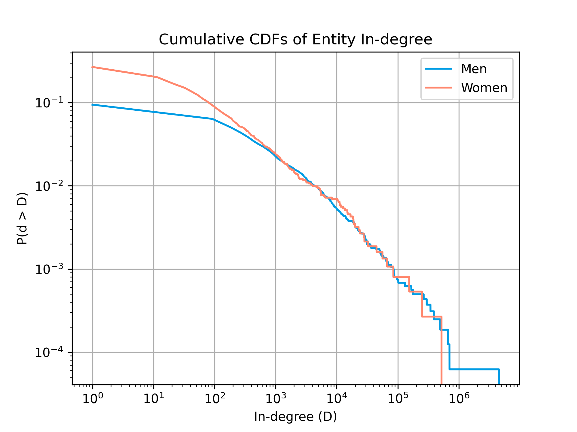
Figure 3.1: The complementary cumulative distribution function of the in-degree distributions of male and female political entities

Student t-tests find a significant difference ($t(13795060)=27.16,p-value<.0001$) between the lengths of comments discussing male ($40.19\pm 37.55$ tokens) and female politicians ($34.23\pm 34.09$ tokens). However, the effect size of this difference (Cohen’s D: 0.16) is negligible.

These results suggest that male and female politicians receive an equal portion of comments. This finding contradicts previous research showing greater coverage of male politicians in media (shor2019). However, unlike this investigation, these studies analyse media attention rather than public interest.

3.4.1.1 Cross-partisan comparison

We find that female politicians receive smaller public interest in all partisan divides of the subreddits. However, left-leaning subreddits show the most equal coverage of male and female politicians. Alt-right discussions contain significantly more comments about male politicians.

When looking exclusively at the partisan subset of the data, we find a smaller portion of comments discussing female politicians in all partisan divides of the subreddits than in the general Reddit conversation. Despite this, left-leaning and alt-right subreddits show relatively more comments discussing female politicians (15.1% and 15.7% of comments, respective to each divide) than that is seen in the right-leaning subreddits (12.4% of comments).

In terms of the number of political entities mentioned, there are fewer entities mentioned in all divides than in the general dataset. However, the overall proportion of male and female politicians is relatively equal across divides. On the left-leaning subreddits, 1.56% of collected female politicians and 1.56% of collected male politicians are mentioned. On the right-leaning subreddits, 1.04% of collected female politicians and 1.09% of collected male politicians are mentioned. 1.85% of female politicians and 1.87% of male politicians seen on the Wikidata database are mentioned on the alt-right subreddit, /r/the_Donald.

	D	p-value
Left	.028	$>.05$
Right	.014	$>.05$
Alt-right	.057	$.007$

Table 3.1: Kolmogorov-Smirnov test results comparing the distribution of comments per political entity across gender

Looking at the plot of the distribution of comments per political entity in Fig 3.2, there is a similar distribution across genders in both the left and right-leaning subreddits. However, there is a significant difference between the genders when looking at the alt-right subreddit, /r/the_Donald. More comments are consistently made about male politicians than female politicians, suggesting male politicians have greater centrality in alt-right political discussions. The results of Kolmogorov-Smirnov tests are reported in Table 3.1.

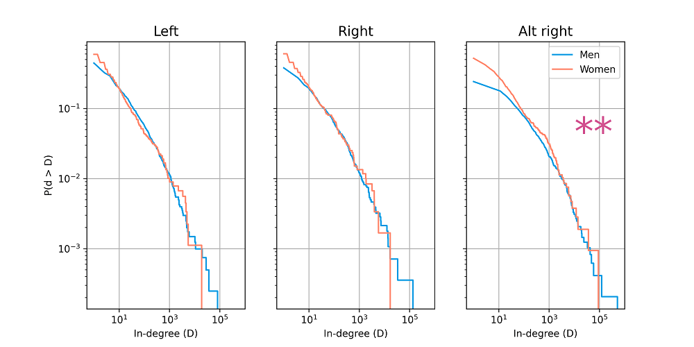
Figure 3.2: The in-degree distributions of male and female politicians across the partisan-aligned subreddits

Comparison		Cohens d
Right, men	Alt-right, women	.44
Right, men	Alt-right, men	.35
Right, men	Left, women	.31
Right, women	Alt-right, women	.30
Left, men	Alt-right, women	.27
Right, men	Right, women	.20
Alt-right, men	Alt-right, women	.19
Right, men	Left, men	.17
Left, men	Left, women	.16
Right, women	Left, women	.14
Left, men	Alt-right, men	.13
Left, women	Alt-right, women	.12
Right, women	Alt-right, men	.08
Left, women	Alt-right, men	.08
Left, men	Right, women	.04

Table 3.2: Effect sizes of the comparisons visualised in Fig 3.3. In bold are the within-partisan group comparisons. The larger value is the value on the left.

Finally, when looking at comment lengths, two-way ANOVAs show significant main effects of partisanship ($F(2,1598999)=11858.9;p<.0001$) and politician gender ($F(1,1598999)=6321.8;p<.0001$), as well as a significant interaction ($F(1,1598999)=172.2;p<.0001$). Post-hoc Tukey HSD tests show that comments about men ($\mu=42.8\pm 61.7$) are consistently longer than those about women ($\mu=31.7\pm 46.0$)($p<.0001;d=.19$). Comments on right-leaning subreddits ($\mu=57.3\pm 81.6$) are significantly longer than those on the left ($\mu=44.1\pm 72.7$)($p<.0001;d=.17$) and alt-right ($\mu=37.1\pm 49.8$) ($p<.0001;d=.36$). Left-leaning comments are longer than those on the alt-right ($p<.0001;d=.13$). Post-hoc Tukey HSD tests found all interaction differences significant ($p<.0001$); they are visualized in Fig 3.3 and their effect sizes are reported in Table 3.2. Though there is a significant difference in comment length in all partisan groups, the effect size is only meaningful in the right-leaning subreddits, though it is small.

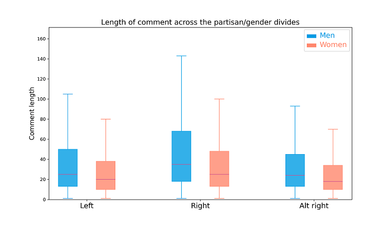
Figure 3.3: The distribution of comment lengths according to gender and subreddit divide.

3.4.2 Combinatorial biases

When female politicians are mentioned, are they mentioned in the context of other women? Or as a token woman in a room of men?

We find that women are more likely to appear in the context of other men than women, but men are also more likely to appear in the context of women than would be expected.

		$g_{given}$
		female	male
$g_{add}$	female	0.14	0.17
	male	1.38	1.11

Table 3.3: Recorded values of $L(g_{given},g_{add})$.

The observed values of $L(g_{given},g_{add})$, as shown in Table 3.3 could, at first, be interpreted to suggest that male political entities are always more likely to be mentioned regardless whether one discusses male or female politicians. However, these values do not account for the relative number of male and female politicians being discussed.

The distribution of $L(g_{given},g_{add})$ of null models of the dataset, as shown in Fig 3.4, shows that the observed values differ significantly from what is seen in random distributions of the data. Female politicians are significantly more likely to be mentioned when discussing either male or female politicians than would be expected from random permutations of the conversations. Male politicians are significantly more likely to be discussed in the context of female politicians and are significantly less likely to be discussed in the context of male politicians than would be expected from the null models. In all instances, the $p$-value of the observed value is below $10^{-5}$. When looking at $L(g_{given},g_{additional})$ values that share their $g_{additional}$ (and, therefore, their marginal probability), it appears that men are more likely to appear in the context of women than other men, and women are slightly more likely to appear in the context of men than other women. These results suggest gender heterophily in the dataset.

Figure 3.4: The recorded value of $L(g_{given},g_{add})$ is plotted in red against the recorded values from null models of the data. A normal probability density function is fitted to the histogram.

3.4.2.1 Cross-partisan comparison

We find, in all partisan divides, men are more likely to appear in the context of women. However, in the left- and right-leaning splits, women are more likely to be observed in the context of other women, rather than men. This is flipped in the case of alt-right subreddits.

		Left		Right		Alt-right
		$g_{given}$		$g_{given}$		$g_{given}$
		male	female	male	female	male	female
$g_{add}$	male	1.17	1.54	1.19	1.42	1.03	1.23
	female	0.17	0.18	0.14	0.16	0.18	0.17

Table 3.4: Recorded values of $L(g_{given},g_{add})$ on the cross-partisan dataset

As can be seen in Fig 3.5, all observed $L(g_{given},g_{add})$ values differ significantly from those seen in the null distribution. In all instances, the p-value is less than $10^{-5}$. Therefore, there is a pattern in the combination of politicians discussed that cannot be approximated with random permutations of the genders. We report the obtained $L(g_{given},g_{add})$ in Table 3.4. In all three partisan groups, $L(female,male)$ is greater than $L(male,male)$. $L(female,female)$ is greater than $L(male,female)$ in left and right-leaning subreddits. In the alt-right subreddit, r/the_Donald, $L(male,female)$ is greater than $L(female,female)$.

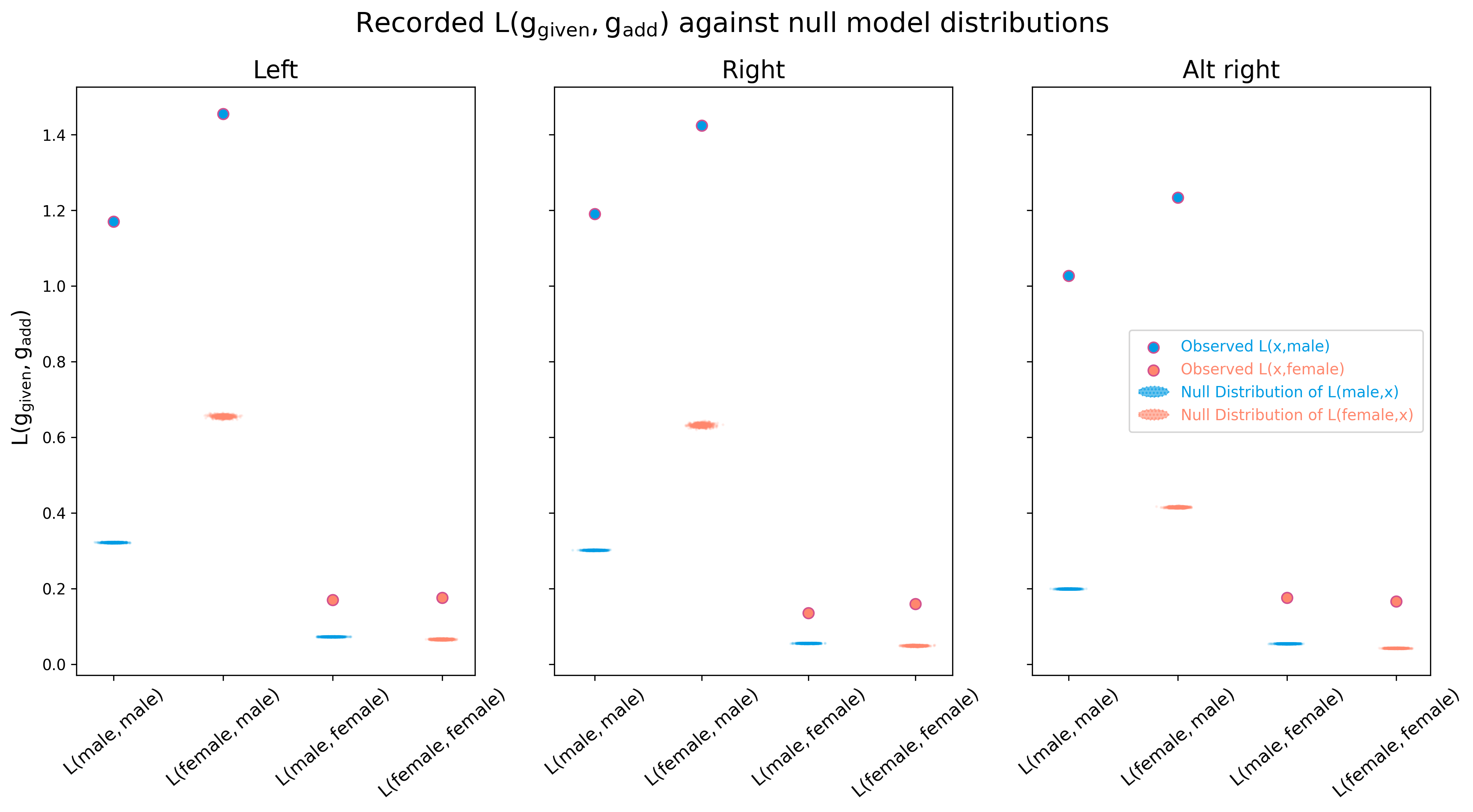
Figure 3.5: The recorded values of $L(g_{given},g_{add})$ plotted against the null distribution clouds of the left, right and alt-right leaning subreddits. Given the large difference in values, we visualize the data as a marked observed value against a distribution cloud of expected values.

3.4.3 Nominal biases

Do people give equal respect in the names they use to refer to male and female politicians?

We find that, while men are overwhelmingly named by their surname, women are much more likely to be named using their full name or given name.
A chi-square test of independence finds a significant relation between subject gender and referent used, $\chi^{2}(3,N=13795685)=2614058.47,p<.0001;V=.44$. The distribution of name choice across gender is pictured in Fig 3.6.

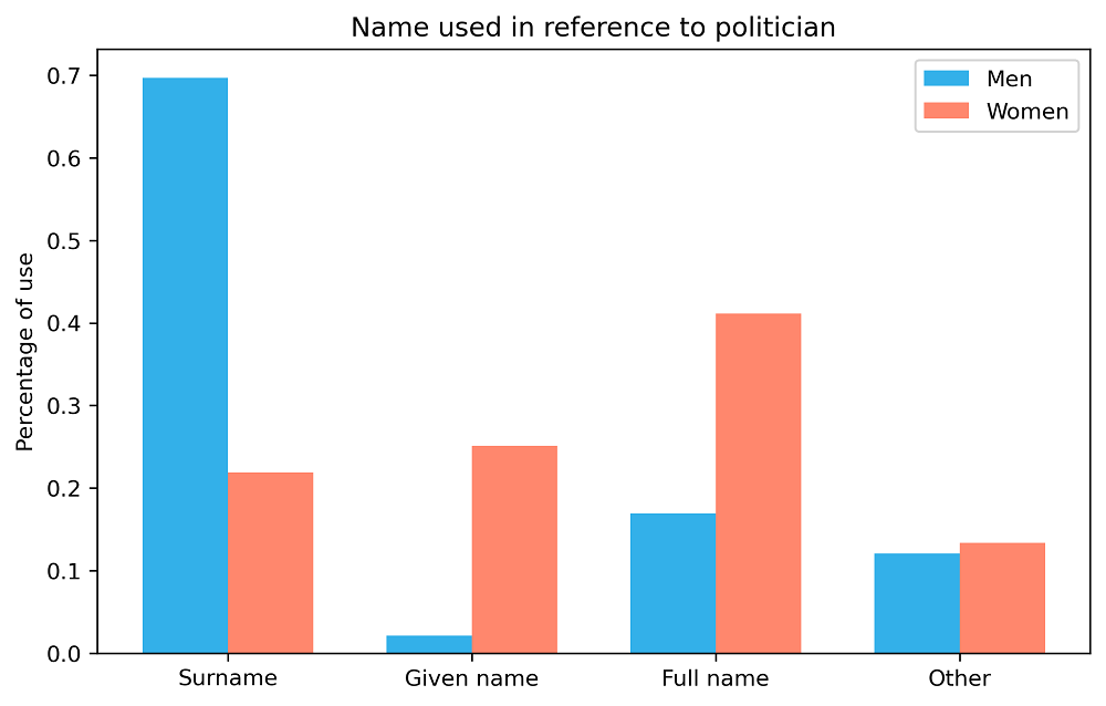
Figure 3.6: The proportion of comments using the various names of an entity, across gender. The “Other” category refers to any other names (i.e. pseudonyms, nicknames, misspellings)

Male politicians are overwhelmingly named using their surname (69.68% of all instances), occasionally via their full name (16.90%), and rarely (2.12%) using their given name. In contrast, women are most often named using their full name (41.14%), followed by their given name (25.09%) and surname (21.90%). Odds ratios indicate that the odds of a male politician being named by his surname are 8.14 times greater than for a female politician ($95\%CI:8.12-8.17;p<.0001$). In contrast, the odds of a female politician being named by her first name are 15.24 times greater than for a man ($95\%CI:15.2-15.3;p<.0001$). Women politicians have odds 3.38 times greater than men to be named using their full name ($95\%CI:3.37-3.39;p<.0001$). Given the vague nature of the “other” category, we do not analyse that value further, but we do note that men and women are equally likely to be referred to by “other” names.

These results suggest that male politicians are more likely to be approached professionally. On the other hand, female politicians are significantly more often mentioned by their given names, which could originate from a lack of respect towards them and, ultimately, gender bias.

3.4.3.1 Cross-partisan comparison

We find that women are much more likely to be named by their given name in alt-right and right-leaning subreddits than in left-leaning splits. However, in all partisan splits, men are significantly more likely to be named via their surname than women.

When looking across the partisan divide, a three-way loglinear analysis produces a final model retaining all effects with a likelihood ratio of $\chi^{2}(0)=0,p=1$, indicating that the highest-order interaction (partisan group x gender x name choice interaction) is significant ($\chi^{2}(6)=3844.066,p<.0001$). Further separate chi-square tests are then performed on two-way interactions. In left-leaning subreddits, there is a significant association between politician gender and choice of nomination ($\chi^{2}(3)=64204,p<.0001,V=.39$); this holds true for right-leaning subreddits ($\chi^{2}(3)=93828,p<.0001,V=.47$) and the alt-right subreddit ($\chi^{2}(3)=416638,p<.0001,V=.50$). There is also a significant association between partisan divide and choice of nomination for female politicians ($\chi^{2}(6)=2874.6,p<.0001;V=.06$), and male politicians ($\chi^{2}(6)=11585,p<.0001,V=.05$). In all three divides, Fig 3.7 shows a similar pattern; Men are named by their surname, but women are named by their full name or given name.

Figure 3.7: An expansion of the use of nameage for politicians across the partisan divide of the data (see along y-axis)

In alt-right subreddits, the odds ratio for a woman to be named by her given name is 18.8 times greater than for a man ($95\%CI:18.5-19.0;p<.0001$). In right-leaning subreddits, the odds are 17.4 ($95\%CI:16.9-17.9;p<.0001$). While the odds for women to be named by their first name are still 8.5 times greater than for men in left-leaning subreddits ($95\%CI:8.3-8.7;p<.0001$); these odds are half of those are seen in the right-leaning and alt-right subreddits. Collapsing surname use and full-name use as a “professional” reference of a politician, the odds of a woman politician being named in a “professional” manner is 1.31 greater in left-leaning subreddits ($95\%CI:1.29-1.33;p<.0001$) and 1.45 greater in right-leaning subreddits than in the alt-right subreddit, /r/the_Donald ($95\%CI:1.42-1.48;p<.0001$). The difference between left and right-leaning subreddits is insignificant ($p>.01$).

When it comes to men, odds ratios show they are 9.5 times more likely to be named by their surname than women in right-leaning subreddits ($95\%CI:9.3-9.8;p<.0001$); the odds are 8.6 ($95\%CI:8.5-8.7;p<.0001$) in the alt-right subreddit, /r/the_Donald. This difference is nearly double the difference seen in left-leaning subreddits; In left-leaning subreddits, the odds for men to be named by their surname are just 5.4 times greater than women ($95\%CI:5.3-5.5;p<.0001$).

3.4.4 Sentimental biases

When people discuss male and female politicians, do they express equal sentiment and power levels in the words chosen?

We find no large difference in sentiment and power attributed to male and female politicians.

Student t-tests of the lexicon-based measure show that comments about male politicians ($N=7190149;\mu=0.325\pm 0.204$) have greater valence than comments about female politicians ($N=980553;\mu=0.314\pm 0.204$) ($t(8170700)=47.78,p<.0001;d=0.05$). Comments about male politicians ($\mu=0.300\pm 0.187$) also show significantly greater dominance than those about women ($\mu=0.285\pm 0.184$) ($t(8170700)=74.31,p<.0001;d=0.08$). It should be noted that, though significant, the effect sizes (as measured via Cohen’s D) of these differences are negligible ($<0.2$).

A chi-square test of independence finds a significant relation between subject gender and referent used, $\chi^{2}(1,N=8170794)=3811.0,p<.0001,V=.02$. Odds ratio tests show that men are 1.17 more likely than women to be in a comment of positive sentiment ($95\%CI:1.16-1.18;p<.0001$). Though this value is significant, the strength of the association (as measured via Cramer’s V) is negligible.

Our results agree with previous studies that find female politicians to have lower dominance and sentiment attributed to them. However, we treat these results with a grain of salt, since the differences are only negligible.

3.4.4.1 Cross-partisan analysis

We find that most differences in sentiment and dominance across the partisan splits are negligible. Men on alt-right subreddits have significantly higher sentiment and dominance than women on left and right-leaning subreddits.

The average comment valence and dominance scores show a bi-modal distribution in all subreddits, as can be seen in Figs 3.8 and 3.9. However, the sample size is sufficiently large to continue with parametric statistical tests.

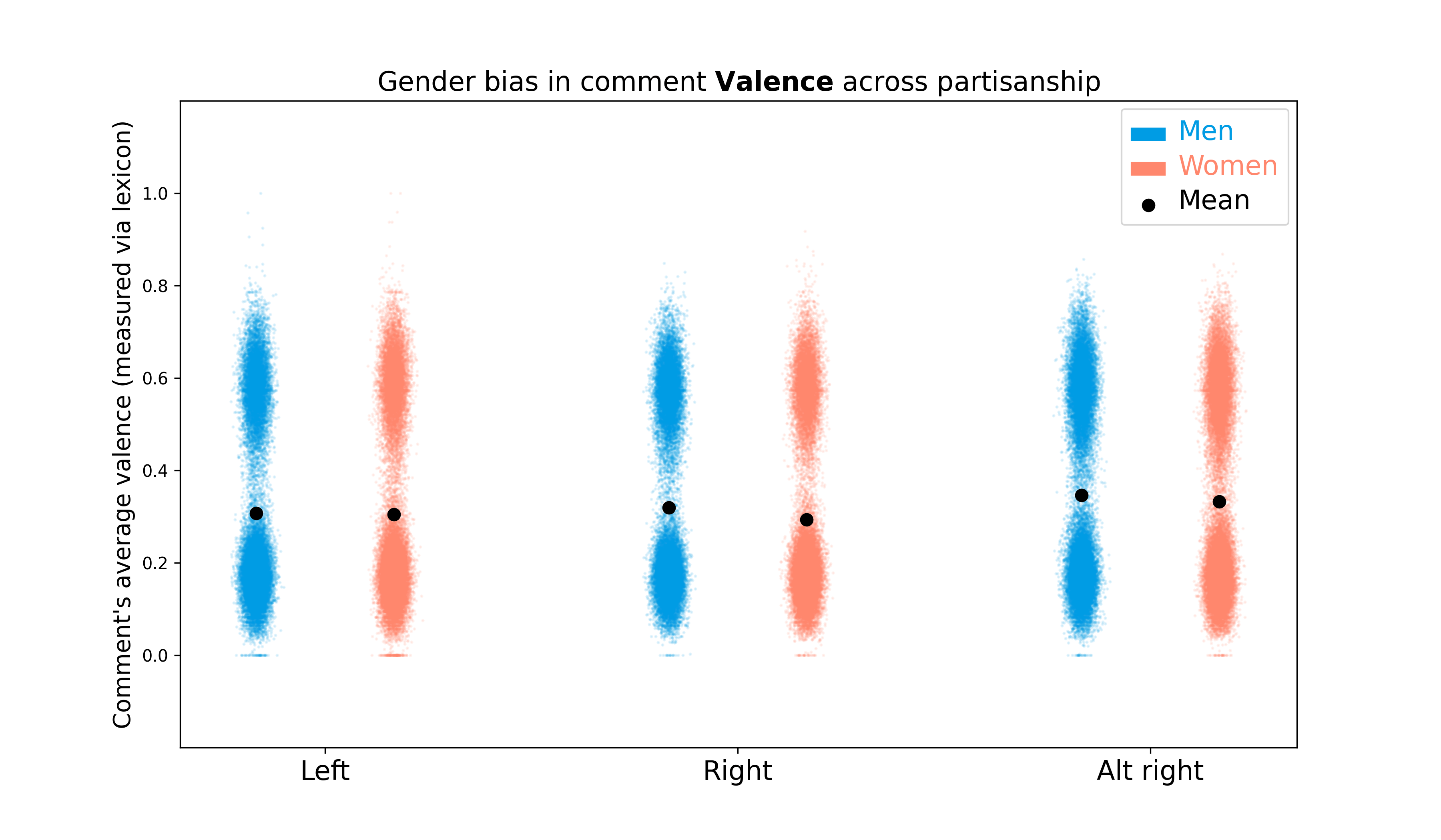
Figure 3.8: Visualization of the distribution of average comment valence across subreddits and topic gender

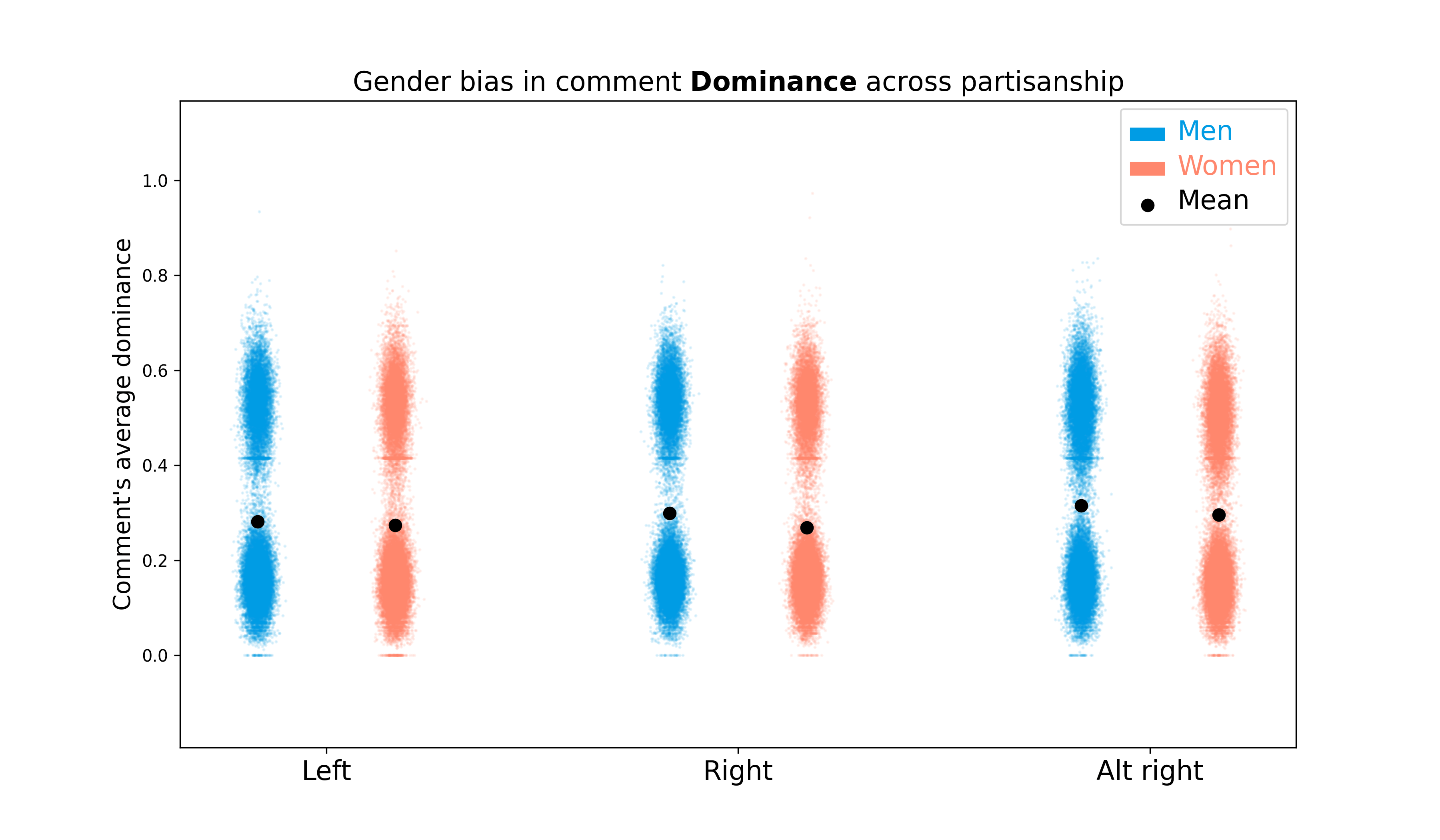
Figure 3.9: Visualization of the distribution of average comment dominance across subreddits and topic gender

Comparison		differences	p-value	Cohen’s d
Alt right, men	Right, women	0.05	$<.0001$	0.25
Alt right, men	Left, women	0.04	$<.0001$	0.2
Alt right, men	Left, men	0.04	$<.0001$	0.19
Alt right, women	Right, women	0.04	$<.0001$	0.19
Alt right, women	Left, women	0.03	$<.0001$	0.13
Alt right, men	Right, men	0.03	$<.0001$	0.13
Right, men	Right, women	0.03	$<.0001$	0.12
Alt right, women	Left, men	0.03	$<.0001$	0.12
Left, women	Right, women	0.03	$<.0001$	0.06
Right, men	Left, women	0.01	$<.0001$	0.07
Alt right, men	Alt right, women	0.01	$<.0001$	0.07
Left, men	Right, women	0.01	$<.0001$	0.06
Right, men	Left, men	0.01	$<.0001$	0.06
Alt right, women	Right, men	0.01	$<.0001$	0.06
Left, women	Right, women	0.01	$<.0001$	0.07
Left, women	Left, men	—–	n.s.	—-

Table 3.5: Results of Tukey-HSD tests on comment mean valance across partisanship and subject gender. The non-negligible effect sizes are bolded.

A two-way ANOVA of average comment valence, as measured via the sentiment lexicon, finds a significant interaction of gender and partisanship ($F(2,1598999)=89.67;p<.0001$) as well as significant main effects of gender ($F(1,1598999)=775.13;p<.0001$) and group ($F(2,1598999)=4299.79;p<.0001$). The data is shown in Fig 3.8 and Table 3.5. Post-hoc Tukey HSD tests show that comments about men ($N=1363556;\mu=.336\pm.209$) have higher valence than comments about women($N=235449;\mu=.323\pm.207$) ($p<.0001;d=0.05$). Comments in left-leaning subreddits ($N=234430;\mu=.307\pm.202$) have significantly lower valence than comments in right-leaning ($N=242075;\mu=.316\pm.202$) ($p<.0001;d=0.04$) and alt-right subreddits ($N=1122500;\mu=.344\pm.211$) ($p<.0001;d=0.18$). Comments in right-leaning subreddits have significantly lower valence than the alt-right subreddit ($p<.0001;d=0.13$). The effect sizes of all differences are negligible. Post-hoc Tukey HSD tests of interactions find a significant difference ($p<.0001$) for nearly all pairs, except ($p>.05$) in the average valence of male and female politicians on left-leaning subreddits. However, many of these effect sizes are negligible.

Comparison		differences	p-value	Cohen’s d
Alt right, men	Right,women	0.05	$<.0001$	0.25
Alt right, men	Left,women	0.04	$<.0001$	0.22
Alt right, men	Left,men	0.03	$<.0001$	0.18
Right, men	Right,women	0.03	$<.0001$	0.16
Alt right, women	Right,women	0.03	$<.0001$	0.15
Right, men	Left,women	0.02	$<.0001$	0.13
Alt right, women	Left,women	0.02	$<.0001$	0.12
Alt right, men	Alt right, women	0.02	$<.0001$	0.1
Right, men	Left,men	0.02	$<.0001$	0.09
Alt right, men	Right, men	0.02	$<.0001$	0.09
Alt right, women	Left,men	0.01	$<.0001$	0.08
Left,men	Right,women	0.01	$<.0001$	0.07
Left,men	Left,women	0.01	$<.0001$	0.04
Right,women	Left,women	0.01	0.002	0.03
Right, men	Alt right, women	0.003	$<.0001$	0.02

Table 3.6: Results of Tukey-HSD tests on comment average dominance across partisanship and subject gender. The non-negligible effect sizes are bolded.

A two-way ANOVA of average comment dominance finds a significant interaction of gender and partisanship ($F(2,1598999)=103.5;p<.0001$) as well as significant main effects of gender ($F(1,1598999)=1960.6;p<.0001$) and group ($F(2,1598999)=3238.5;p<.0001$). The data is shown in Fig 3.9 and Table 3.6. Post-hoc Tukey HSD tests show that comments about men ($\mu=.258\pm.160$) have higher dominance than comments about women($\mu=.244\pm.157$) ($p<.0001;d=0.10$). Comments in left-leaning subreddits ($\mu=.280\pm.184$) have significantly lower dominance than comments in right-leaning ($\mu=.295\pm.187$) ($p<.0001;d=0.08$) and alt-right subreddits ($\mu=.312\pm.190$) ($p<.0001;d=0.17$). Comments in right-leaning subreddits have significantly lower dominance than the alt-right subreddit ($p<.0001;d=0.09$). Post-hoc Tukey HSD tests of interactions find significant differences ($p<.01$) for all pairs, though many of the effect sizes are negligible.

A three-way loglinear analysis of the classifier-output sentiment labels produces a final model retaining all effects with a likelihood ratio of $\chi^{2}(0)=0,p=1$, indicating that the highest-order interaction (partisan group x gender x sentiment label) is significant ($\chi^{2}(7)=9141.02,p<.0001$). Further separate chi-square tests are then performed on two-way interactions. In left-leaning subreddits, there is a significant association between politician gender and comment sentiment ($\chi^{2}(1)=106.96,p<.0001,V=.02$); this holds true for the alt-right subreddit ($\chi^{2}(1)=2194.3,p<.0001,V=.04$), but not right-leaning subreddits ($\chi^{2}(1)=2.2,p>.05$). There is also a significant association between partisan divide and comment sentiment label for female politicians ($\chi^{2}(2)=1039.2,p<.0001;V=.07$), and male politicians ($\chi^{2}(2)=5032.8,p<.0001,V=.06$).

In left-leaning subreddits, men are 0.87 times as likely as women to be named in a comment with positive sentiment ($95\%CI:0.85-0.90;p<.0001$). In contrast, in the alt-right subreddit, men are 1.34 times more likely to be described in positive sentiment than women ($95\%CI:1.33-1.36;p<.0001$) However, while we see significant differences, the strength of these associations, as measured via Cramer’s V, are minimal. The frequencies are visualized in Figure 3.10.

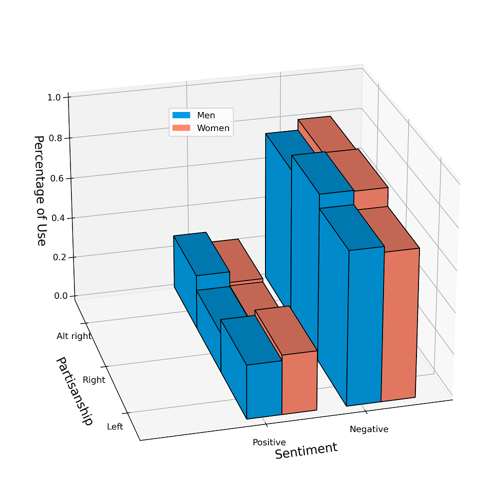
Figure 3.10: The output of the sentiment classifier is compared across gender and subreddit partisanship. Though gender differences are significant in both left-leaning and alt-right subreddits, the association strength is negligible, like the differences measured via the sentiment lexicon.

3.4.5 Lexical biases

When people discuss male and female politicians, how do the words they use to describe them differ?

We find highly female-biased words are more likely to be about body, clothing or family-related descriptors than male-biased words. In contrast, highly male-biased words are more likely to be profession-related.

Firstly, we investigate the differences in results between the traditional and improved PMI method, to show the efficacy of the entity-based approach. Thereafter, we go into the general gender biases that can be seen in the dataset. Again, we conclude with a cross-partisan analysis. Given the source of this dataset, there may be some offensive and/or explicit words in the following sections and associated appendices.

Traditional PMI		PMIe
truancy	1.969493	chairwoman	1.421482
react	1.936892	pantsuit	1.407579
somalian	1.93603	matriarch	1.351489
cherokee	1.927183	facelift	1.313268
cheekbone	1.92447	menopausal	1.313268
pantsuit	1.901174	harpy	1.313268
beetus	1.893833	scarf	1.29525
directory	1.888102	clitoris	1.264478
spokeswoman	1.874243	clit	1.264478
jamaican	1.866066	brunette	1.264478

Table 3.7: Results of the Traditional PMI on the left. The entity-based technique is on the right. See the elimination of ethnicity-based terms on the right, while some words like “pantsuit” are still retained in the top 10.

The top 10 female-associated words obtained through traditional and entity-based PMI methods are shown in Table 3.7. While also including explicitly gendered words (e.g. ‘chairwoman’), the traditional PMI method attributes a high PMI value to many ethnicity-centered words, such as ‘Somalian’ and ‘Cherokee’. These should not be gendered words. They are, however, heavily associated with specific popular politicians, Somalian-born US Representative Ilhan Omar and Senator Elizabeth Warren, who have faced criticism about claims of Cherokee heritage.

In contrast, the entity-based approach removes many of these obviously confounding words related to ethnicity. In addition, many obviously gendered words are prioritized (e.g. “chairwoman” and ‘menopausal’). Though no longer on the top-10 list, ‘spokeswoman’ still has a high female PMIe (1.83, #17 on the list). Less-obviously gendered terms are retained in both lists (e.g. ‘pantsuit’), but more appear in the PMIe word list. These terms are further explored in the next sections.

3.4.5.1 General gender comparison

Male-bias		Female-bias
bloke	0.171301	chairwoman	1.421482
wanker	0.166013	pantsuit	1.407579
prince	0.160944	matriarch	1.351489
lawful	0.159782	facelift	1.313268
turkish	0.151414	menopausal	1.313268
madman	0.147948	harpy	1.313268
unchecked	0.146697	scarf	1.29525
punchable	0.145394	clitoris	1.264478
dickhead	0.142614	clit	1.264478
truck	0.142614	brunette	1.264478

Table 3.8: The top-10 male and female-biased words in the dataset, using the entity-based PMI approach

Using this entity-based PMI approach, we now turn to the words in the dataset that have a high gendered PMI value. The top 10 for each explored gender with their PMI value for that gender are shown in Table 3.8. The remainder of the words, and their annotated senses, are visible in S2 Table in §3.7.2. It is interesting to note that the highest PMI values for the male-biased words are quite low and near zero; this may be due to the overwhelming existence of more male entities in the dataset. However, despite this near-zero number, there are some obviously gendered words (e.g. ‘prince’) on the list. An ethnicity-related term remains the male-biased PMIe list (‘turkish’). However, this may be owed to actual gender bias, given Turkey’s low ranking on the gender gap report (GGGR), especially within political empowerment. Within the top-100 list of male and female-biased words, all PMI values are above 0.10.

Though we hoped to use lexica to analyse the larger dataset, the Slang SD, NRC, and Supersenses lexica together only cover 32.5% of the top 100 words for either male or female bias. Therefore, we rely on hand-coded senses and sentiments. The annotators achieve a Cohen’s Kappa Agreement of 0.618 on the Handcoded Sentiment and 0.620 on Senses on a subsample of 50 words, suggesting substantial agreement.

A chi-square test of independence is performed to examine the relation between gender and the distribution of word senses. The relation between these variables is significant ($\chi^{2}(7,N=200)=46.29,p<.0001;V=.50$) and their distributions are visualized in Fig 3.11. Overall, there are few positive words in both the top male and female-biased words. Negative labels make up a high portion of both male and female-skewed words; Odds ratio tests show that the odds of finding negative labels in male-biased words are not significantly higher than in female-biased words ($p>.05$). In addition, the odds of female-biased words containing attribute-related descriptors (18%) are not significantly greater than male-biased words (13%) ($p>.05$). However, there is a big disparity between the genders in the remaining categories. The odds of male-skewed words containing profession and belief-related descriptors (20%) are 2.98 greater than female-skewed words (7%) ($95\%CI:1.16-7.22;p<.05$). In contrast, the odds of female-skewed words containing body-related descriptors (19%) are an estimated 8.94 times greater than for male-skewed words (3%) ($95\%CI:2.5-31.4;p<.0001$). In addition, while there are 0 male-biased words related to their clothing and family, both categories are represented more in female-biased words (7% and 6%) than words related to their own profession (4%).

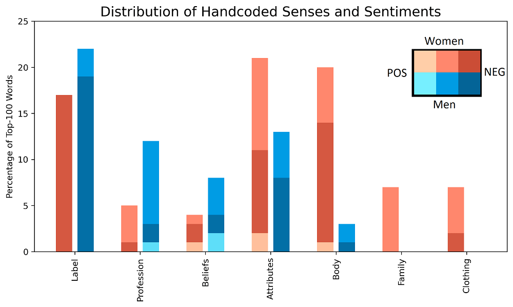
Figure 3.11: The distribution of the hand coded senses and sentiments across words with high gender bias. Words coded as “Other” are not included.

Hence, words associated with female politicians are often irrelevant descriptors of their appearance or family. This treatment does not apply to male politicians who are described in relation to their profession and politics in general. These results suggest presence of gender bias on a lexical level.

3.4.5.2 Cross-partisan comparison

We find the alt-right subreddits contain much more body-related descriptors for female politicians than left or right-leaning subreddits.

When comparing the hand-coded senses and sentiments of the top gendered words in the partisan-divided groups of subreddits, as shown in Fig 3.12, there is a visual difference in which descriptors play larger roles across the genders. While body-related descriptors appear for women in all three groups, they do not appear in either of the three male-skewed lists. However, odds ratio show that body-related descriptors have 8.00 times greater odds of being highly female-biased on the alt-right subreddit than on left-leaning subreddits ($95\%CI:1.75-36.6;p<.01$). There are no other significant differences in body-related descriptors between subreddit groups ($p>.05$). Instead, on the left and right-leaning subreddits, women are more described by their attributes. The odds of woman-related words being attribute-related are 3.49 times greater on the left-leaning and right-leaning subreddits than on the alt-right subreddit ($95\%CI:1.15-10.63;p<.05$). There is no difference between the left and right-leaning subreddits.

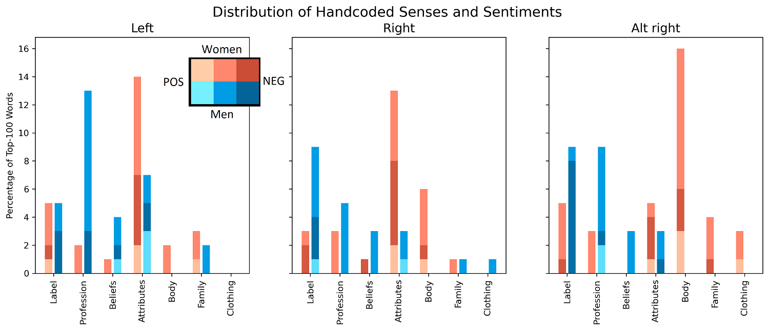
Figure 3.12: The word sense distributions across the most gender biased words along the partisan-leaning subreddits

On the other hand, in left-leaning subreddits, male-skewed words have 8.07 greater odds of containing profession- and belief-related words than female-skewed words ($95\%CI:2.19-29.8;p<.001$). The odds in the alt-right subreddits are almost half of that: 4.95 ($95\%:1.30-18.8;p<.05$). The odds are not significantly different in right-leaning subreddits ($p>.05$). However, looking at the distribution, it appears that these differences are due to fewer profession-related words appearing on the male-skewed list, not more female-biased profession-related words.

3.5 Discussion

3.5.1 Biases in the general community

In our investigation of coverage biases (§3.4.1), we find a generally equal amount of public interest in both male and female politicians; male and female politicians generate equivalent distributions of comments (Fig 3.1). Furthermore, the differences in the proportion of possible politicians discussed (a slightly greater proportion of female politicians are discussed) and comment length (comments about female politicians are, on average, 6 tokens shorter than those for male politicians) are negligible. While previous studies have shown longer articles and greater coverage devoted to male figures (field2020controlled; nguyen2020), especially male politicians (shor2019), these are not measures of the public’s interest, but that of the media’s (which may be affected by the intended audience, sponsors, and an editorial hierarchy). In contrast, our measures of coverage are measures of general public interest. This is interesting, given that another study of public interest, as measured via Wikipedia article views, suggests that, though interest is generally higher for female figures than for male figures, this is not the case for politicians (shor2019). We find equal public interest, likely as we measure a higher standard of engaged interest. However, our comparisons of coverage and public interest are done quite simply, without consideration of the politician’s age and level of position. These two factors are likely to affect the amount of attained public interest (and, due to known gender biases, are most likely to act against female politicians, as they are more likely to have shorter careers and stay in lower levels of hierarchy (cotter2001; folke2016; hagan1995gender)). Therefore, there remains the possibility that our finding of equal public interest in politicians is a conservative estimate, and there may be even greater public interest in female politicians to equivalent male politicians.

Interestingly, the null models conducted in this investigation of combinatorial biases (§3.4.2) suggest that female politicians are more likely to be mentioned in the context of both other women and men than would be expected by their presence in the dataset (Fig 3.4). Though one may expect to see the Smurfette principle in practice (pollitt1991), or, at least, gender homophily, it is surprising to see that women appear more often than would be expected in both men and women-containing conversations, and they are discussed in a manner that cannot be simulated with random permutations. Interestingly, when comparing values with shared marginal probabilities, it appears that men are more likely to appear in the context of women than other men, and women are more likely to appear in the context of other men. If anything, this suggests heterophily within the network.

Starker biases begin to appear when one looks within the text rather than the overall structure, as we see in nominal (§3.4.3), sentimental (§3.4.4)and lexical (§3.4.5) analyses. Male politicians are more likely to be named professionally than female politicians. Instead, women are overwhelmingly more likely to be named using their given name than men (Fig 3.6). This validates many claims about female professionals being referred to using familiar terms, diminishing their authority and perceived credibility and widening the existent gender gap (atir_ferguson_2018; margot_2020). Overall, female politicians are still most commonly referred to by their full name. However, it is important to note that the co-reference resolution step biases towards extending the longest observed name down the entire cascade. Therefore, the use of a full name may be overrepresented in this dataset. In addition, the named entity linker may miss many references to politicians under unknown nicknames or common first names, thereby excluding these comments from these analyses.

While female politicians have lower sentiment and dominance attributed to them in comments, the effect sizes are not meaningful. This is also seen when sentiment is measured via a classifier output. This is interesting, given that previous studies have shown that women generally have more positive sentiment and low dominance (li2020content; fast2016shirtless; voigt-etal-2018-rtgender) attributed to them, a concept referred to as benevolent sexism (glick1996). It could also be expected, from previous studies, that more negative sentiment would be expressed towards women, given persisting implicit prejudices against female authority figures (rudmankilianski2000). However, in our examination of sentiment, we do not see the manifestation of neither hostile nor benevolent sexism at play. It is interesting to note that, in the lexicon-based method, both the valence and dominance level comment averages show a bi-modal distribution– other studies using this lexicon show a normal distribution (mohammad-etal-2018-semeval), which leads us to wonder from where the bimodality arises. Possibly, the two peaks belong to opposing party members (for example, the more positive peak corresponds to politicians of the same political alignment as the poster).

When it comes to the PMI-based lexical bias investigation, there is a clear difference in the most male and female-gendered words (Tables 3.7–3.8). Surprisingly, neutral and negative labels are equally likely to be heavily attributed to men or women. This echoes our investigation into sentimental biases; we do not see evidence of benevolence or hostility towards female politicians. However, there are still stark differences in how men and women are described. Profession and political belief-related terms show a heavy male-skew, echoing results of other studies (garg2018stereotypes; mertens2019; wagner2015its). This is not necessarily the case for women. Highly female-gendered words are often about irrelevant descriptors: their body, their clothing, and their family. This matches many gender bias studies which show that the public and media take a more personal interest into female professionals (mertens2019; hoyle-etal-2019-unsupervised; wagner2015its; Devinney1509712; li2020content; fu2016tiebreaker; rudinger-etal-2017-social). These results also match similar studies showing an overwhelming amount of body-related descriptors being attributed to women (hoyle-etal-2019-unsupervised; garg2018stereotypes; field-tsvetkov-2020-unsupervised; rudinger-etal-2017-social). However, while other studies show more positive body-related descriptors for women (hoyle-etal-2019-unsupervised), we find predominately negative or neutral body-related descriptors. Though attribute-related descriptors appear in both male- and female-biased word lists, they are the only professional standards to which women are held. Not their policies or professional qualifications, but their other attributes: their elegance and their bossiness, if not their looks. The biases faced by female politicians lay outside benevolent or hostile sexism; they involve more nuanced societal expectations around their appearance and their personality. Finally, it is interesting to note that, Table 3.8 shows that even clearly male-biased words (e.g. “prince”) have significantly lower PMI-values than female-biased words. While this likely owes to the predominance of male-centric comments in the dataset, it echos the recurrent theme in technology that men are the “null” or standard gender (fox_johnson_rosser_2006). This is an unintentional outcome of training algorithms on an imbalanced dataset, as one runs the risk of perpetuating existing biases.

3.5.2 Biases across the political spectrum

The sub-community nature of the dataset allows us to investigate how these observed biases change along the partisan line. In the left-leaning subreddits, there is what could be interpreted as the most egalitarian treatment across the genders, which coincides with expressed left-leaning values. These subreddits showed the most equal coverage of male and female politicians, in terms of the politicians mentioned, politician in-degree distribution, and comment lengths (§3.4.1.1). The odds of a female politician being named using her given name are half those seen in the right-leaning partisan divides (Fig 3.7). In addition, the left-leaning subreddits are the only subset that does not show a significant difference in sentiment between male and female politicians, though the difference observed in other interest groups is negligible (3.4.4.1). Compared to the two right-leaning divides, body-related descriptors are the least represented in the heavily female-biased words. However, some gender disparity still remains; male-skewed terms on left-leaning subreddit are overwhelmingly related to their profession and political beliefs, unlike heavily female-biased words (Fig 3.12). Men are held to a certain set of professional standards, whereas women politicians are described by their general attributes. Therefore, while left-leaning posters may discuss non-superficial attributes in female politicians, these attributes may not necessarily be politically relevant but may showcase a different standard of qualifications that women are expected to uphold (e.g. trustworthiness, capability, likeability) instead of the professional qualities with which male politicians are described (watson1988).

When it comes to the right-leaning subreddits, there are some conflicting results. The distribution of activity generated per entity is equal between men and women, though there are fewer comments about women, and fewer female politicians mentioned (§3.4.1.1). This group of subreddits show the greatest divide in the number of female and male politicians mentioned. In addition, comments about these female politicians are, on average, 10 tokens shorter, though the effect size is small. Taken together, it appears that participants in right-leaning subreddits have, overall, slightly less active interest in female politicians. Despite this lower engagement, however, female politicians are still treated with respect; they are equally as likely to be referenced in professional terms as in left-leaning subreddits, though women are twice as likely to be referenced by their given name than in those subreddits (Fig 3.7). Attribute-related descriptors make up a bigger proportion of heavily female-biased descriptors than body-related ones, and both profession and political-belief-related descriptors are equally as likely to be female- and male-biased, unlike as seen the other political divides (Fig 3.12). However, this appears to arise from fewer male-biased profession-related descriptors, not more female-biased ones. Ultimately, in right-wing fora, the engagement in conversation about female politicians, though potentially smaller, remains professionally relevant.

Finally, in the informal alternative-right subreddit, /r/the_Donald, there are much starker differences. Though many female politicians are mentioned, there is a significant difference in the level of interest generated by the politicians (Fig 3.2). Unlike the other political divides, combinatorial investigations suggest that women appear to be slightly more likely to be discussed in conjugation with men, rather than other women (Fig 3.5). When mentioned, female politicians are twice as likely to be named via their given name than the left-leaning subreddits, and they are almost 1.5 times less likely to be named using their full or surname than in both other political subreddit groups (Fig 3.7). The words most attributed to female politicians are overwhelmingly related to their bodies, rather than their profession, beliefs or other supra physical attributes (Fig 3.12). This suggests an overall disregard for female politicians; not only is there less active interest in the politicians, but, when they are discussed, female politicians are not as often discussed with respect as professionals but rather in relation to their bodies.

3.5.3 Limitations and Contributions

There are some limitations in how far the cross-partisan analyses can be interpreted. Firstly, the obtained results cannot differentiate whether the observed differences are general patterns in the behaviour of the participants or differences in the actual politicians being discussed in the subreddits. Perhaps female politicians who prefer the use of their given name and have legitimate, professional reasons to be described with body-related terms (e.g. disease awareness activists) are more likely to be discussed on the alt-right. Our grouping of these subreddits may also affect the observed results. Even within similar communities, gender biases and community norms may differ, creating a noisy sample (raut_2020). In addition, the population of the left-leaning and right-leaning subreddits may not be as disparate as those of the right-leaning and alt-right subreddits. Given the overlap in political beliefs, the population of posters may also overlap. The observed differences in this study may be generated by political viewpoints or other differences between the subreddits (e.g. moderation level or formality). These analyses simply showcase the language that is acceptable within the community, after moderation, which may differ both across community formality and partisanship. Other studies simply investigate the right-left divide (mertens2019). To ensure that the overwhelming presence of Trump-related comments in the dataset did not result, in S3 Text in §3.7.3, we validate that we continue to see similar patterns of results even with the removal of all Trump-related comments from the data-set. Therefore, the biases we describe are not necessarily simply differences between women and Donald Trump but gender differences that can be applied more generally across politicians. We continue to see the same pattern of results even in the alt-right data, which is heavily influenced by Donald Trump. Therefore, we would like to stress that these observed biases are not necessarily guided by certain prominent figures but are reflective of biases within the general ideologies.

While Reddit users make up a wider variation of people than news journalists, Wikipedia editors, and book authors (wagner2015its; Wagner_2016; hoyle-etal-2019-unsupervised; garg2018stereotypes; shor2019), the population from which many other studies draw their data, the Reddit user distribution is still skewed towards white, college-educated men (barthel_stocking_holcomb_mitchell_2016), though we take efforts to increase the dataset’s diversity. In addition, our entity-linker showed only 50% accuracy when linking to female politicians, giving us fewer comments about female politicians. This is a clear gender bias in the data-processing step; We suspect that, given that female politicians appear relatively likely to be referenced by their given name, surname or full name, this may be a source of noise for the entity-linker that contributes to its inaccuracy. More investigation on how gender bias emerges in these intermediate processing steps is warranted, as it likely contributes to some skew within the dataset. Other processing steps may contain gender biases or may affect the measured biases; the coreference resolution pre-processing step likely biases our dataset towards more instances of full names in the comment text. Many NLP tools are trained on formal text (i.e. books, newspapers) and may not be as effective on social media text, like that seen in Reddit. To avoid these issues, we choose simpler pre-processing steps and avoid the use of parsers, but errors still arise from the pre-processing that is conducted, given the text medium.

Due to the limitation in the multilingual pre-processing tools required for this investigation, we focused our investigation in English. However, other studies have found that both linguistic and extra-linguistic biases can vary heavily across language (wagner2015its). Therefore, we cannot necessarily generalise our findings across languages and non-English-speaking cultures. While one could translate all text into a single language for analysis, this runs the risk of amplifying biases present in machine (or human) translators, rather than in the source language. Similar yet multilingual studies would benefit from multilingual entity linker and coreference resolution tools to create the required dataset. Most of the described analyses should be feasible in a variety of other languages. The spaCy dependency parser used to determine descriptors for the lexical bias assessment is available in 21 different languages. However, both the lexicon and classifier-based methods for sentimental bias assessment are limited to English text. While we cannot find any publicly available pre-trained multi-lingual sentiment classifiers, a lexicon-based method could train language-specific VADER-based lexica for the languages of interest (hutto2014). To allow score comparability between languages, baglini2021 recommend training a normalization algorithm across the included languages. However, this approach may require validation of the lexica by one or more native speakers of the languages.

A major output of this investigation is the dataset created in the process. Other, earlier studies of gender bias rely on implicit psychological techniques or sociological methods (Greenwald1998MeasuringID; rudmankilianski2000; nosek2011-implicit); however, they are limited in their sample size, their sampling method (as participants are aware they are being watched), and possible researcher bias. The resulting 10 million comment Reddit dataset allows for a powerful measure of popular social gender bias. Other large studies of gender biases have relied on those present in polished media, such as news coverage and literature (hoyle-etal-2019-unsupervised; field2020controlled; fast2016shirtless; li2020content; nguyen2020; shor2019). However, these are sources where the final product is carefully manufactured to appeal to an audience and do not necessarily provide a measure of general society’s biases. Many other studies using social media data exist, such as those on Twitter (mertens2019; PAMUNGKAS2020102360; sap-etal-2020-social) or Facebook (voigt-etal-2018-rtgender; field-tsvetkov-2020-unsupervised). However, Twitter data is limited by the character limit, and Facebook studies focus on text and language addressed to a gender, not about them, which can affect presented biases (field-tsvetkov-2020-unsupervised; dinan-etal-2020-multi). Other studies on gender biases using Reddit data exist (farrell2019; raut_2020), but this presented dataset allows the exploration of biases within politics, distinct from other gender biases. The delineation of these specific gender biases is interesting for a diverse range of subjects: computer science, linguistics, political science, and gender studies. To contribute to the uncovering of these biases, we provide the code and dataset for future use in studies.

3.6 Conclusion

In this paper, we present a comprehensive study of gender bias against women in authority on social media. We curate a dataset with 10 million Reddit comments. We investigate hostile and finer forms of bias, i.e. benevolent sexism. To this end, we employ different types of bias to assess the nuanced nature of gender bias. We have been able to show a range of structural and text biases across two years of political commentary on the curated Reddit dataset. Though we see relatively equal public interest in male and female politicians, as measured by comment distribution and length, this interest may not be equally professional and reverent; female politicians are much more likely to be referenced using their first name and described in relation to their body, clothing and family than male politicians. Finally, we can see this disparity grow as we move further right on the political spectrum, though gender differences still appear in left-leaning subreddits.

Future work

Future investigations on gender biases could first match politicians on age, hierarchical level and other potentially confounding factors, by which female politicians are disproportionately affected (field2020controlled). This could also allow the investigation of other existing biases, such as those against different races or gender biases. Biases, such as racism and sexism, often interact. Elucidation of these interactions is difficult but is only possible with the use of computational techniques, such as Field et al’s use of matching algorithms to show the interplay of gender, racial and sexual biases on Wikipedia (field2020controlled). Given that all linked entities are first linked to Wikipedia pages before Wikidata IDs, a similar technique could be employed on our data, as the traits used in Field et al’s matching algorithm would be accessible from the mapped Wikipedia pages.

Future investigations into combinatorial biases, nominal biases, and sentimental biases could also benefit from modifications. An in-depth investigation into combinatorial biases could utilise higher-order networks (with consideration of the combinatorial issues in calculating homophily) or compute Monte Carlo simulations to investigate hypothetical causes for the observed conditional distribution. Investigations of nominal biases could be expanded to include mention of a politician’s post, also a signal of respect for political authority, or to further investigate usage of nicknames, which may require hand-curated lexica of common nicknames for mentioned politicians (to avoid the accidental inclusion of misspellings). In addition, the causes of the bi-modality of the observed distribution of comment sentiment can also be further investigated. The entity-based PMI tactic could also be expanded to include document and entity-based significance measures (damani-2013-improving). The inclusion of these updates may lead to more nuanced results than the ones reported in this investigation.

Finally, a benefit of this dataset is its applicability for a variety of other comparisons not assessed in this study, possibly thanks to the structure of Reddit. These include more cross-community comparisons, tracking user affiliations to increase the dataset size, or longitudinal comparisons. We conduct one example of a cross-community comparison with a cross-partisan comparison. However, further investigations could include inter-country comparisons, intra-generational studies (via investigation of the comments from /r/teenagers), and cross-lingual studies. Future studies could try to augment the dataset for comparisons of smaller subreddits, such as /r/MensRights or /r/feminisms. Researchers could query regular posters on these subreddits and find their posts on other larger subreddits (e.g. /r/politics, r/news). Their status as regular posters on one niche subreddit can identify them as likely belonging to one ‘group’, and their behaviour on larger subreddits could be added to the comparison. This carries the assumption that one’s participation in a subreddit is a signal of a constant belief of that user, which may not always be applicable and must be verified. A user who once posted in a misogynist space two years ago may no longer carry misogynist views. In the case of regular posters, one could investigate how a user’s behaviour may change between subreddits as a proxy to show how biases may change across communities. Lastly, time periods could be compared to assess changes in biases over time.

Acknowledgements

We would like to thank Dr. Jonas J. Juul for his advice and feedback in the calculation of combinatorial biases. We would also like to acknowledge those that played a role in the annotation process: Ivo, Laura, and Vivian, for their help in attributing word-senses to the terms extracted from this data-set.

This work is partly funded by Independent Research Fund Denmark under grant agreement number 9130-00092B.

3.7 Appendix

3.7.1 S1 Table. Subreddits Included.

Subreddit	Number of comments	Partisan-affiliation
politics	9744853	—
The_Donald	1664335	alt-right
news	556783	—
neoliberal	340533	left
canada	285667	—
Libertarian	207109	right
Conservative	200772	right
unitedkingdom	197881	—
europe	158342	—
australia	107966	—
india	87367	—
democrats	53381	left
ireland	40964	—
teenagers	33311	—
newzealand	32847	—
socialism	18241	left
TwoXChromosomes	15734	—
MensRights	13664	—
Republican	13014	right
Liberal	10503	left
uspolitics	8873	—
SocialDemocracy	1977	left
alltheleft	837	left
feminisms	108	—

Table 3.9: Subreddits Included.

3.7.2 S2 Table. PMI Annotations.

Female-bias words	Sense	Sentiment	Male-bias words	Senses	Sentiment
chairwoman	Profession	0	bloke	Label	0
pantsuit	Clothing	0	wanker	Label	-1
matriarch	Family	0	prince	Profession	0
facelift	Body	0	lawful	Belief	1
menopausal	Attribute	-1	turkish	Other	0
harpy	Label	-1	madman	Attribute	-1
scarf	Clothing	0	unchecked	Attribute	-1
clitoris	Body	0	punchable	Body	-1
clit	Body	-1	dickhead	Label	-1
brunette	Body	0	truck	Other	0
wench	Label	-1	businessman	Profession	0
hind	Body	-1	informant	Other	0
childless	Family	0	inflation	Other	-1
skank	Label	-1	jock	Label	-1
misandrist	Attribute	-1	sovereign	Other	1
hubby	Family	0	chode	Label	-1
cheekbone	Body	0	prick	Label	-1
boogeywoman	Label	-1	cure	Other	1
btch	Label	-1	envoy	Profession	0
brooch	Clothing	0	testicle	Body	0
nosedive	Other	-1	ruler	Profession	0
driven	Attribute	0	worm	Other	-1
conceal	Other	-1	republic	Belief	0
elegance	Attribute	0	discovery	Other	1
ballz	Label	-1	douchebag	Label	-1
numerical	Other	0	constitutionalist	Belief	0
goddess	Body	1	urgent	Other	0
blouse	Clothing	0	lad	Label	-1
interjection	Other	0	hereby	Other	0
succubus	Label	-1	mafia	Other	-1
heroine	Attribute	1	bluster	Attribute	-1
aunty	Family	0	imperialism	Belief	-1
equipped	Attribute	0	kiddie	Label	-1
progressiveness	Belief	0	undisclosed	Other	-1
dependency	Other	0	kisser	Attribute	-1
congresswoman	Profession	0	sleazeball	Label	-1

Female-bias words	Sense	Sentiment	Male-bias words	Senses	Sentiment
hag	Label	-1	errand	Other	0
fuckable	Body	-1	gatekeeper	Attribute	0
frumpy	Body	-1	chairman	Profession	0
racy	Clothing	-1	longstanding	Other	0
ovary	Body	0	shitbird	Label	-1
smokey	Other	0	douche	Label	-1
crone	Body	-1	fanboy	Label	0
dyke	Label	-1	congressman	Profession	0
suffragette	Belief	1	excess	Other	0
businesswoman	Profession	0	diddler	Label	-1
42nd	Other	-1	manifestation	Other	0
radiant	Attribute	1	utopia	Belief	1
charmed	Attribute	0	federalist	Belief	0
mediator	Attribute	0	meddling	Attribute	-1
throatedly	Attribute	-1	lowlife	Label	-1
regal	Attribute	0	alley	Other	0
skincare	Body	0	ukraine	Other	0
biatch	Label	-1	chancellor	Profession	0
wonkiness	Other	-1	affect	Other	-1
finely	Attribute	0	offshore	Other	-1
statesperson	Attribute	0	philosophical	Attribute	0
memelord	Label	-1	grim	Attribute	-1
stepmother	Family	0	wimp	Label	-1
peopel	Other	0	rain	Other	0
dementor	Label	-1	crypto	Other	0
cackle	Attribute	-1	henchman	Profession	-1
shrew	Label	-1	overhaul	Other	0
mudslinging	Attribute	-1	palace	Other	0
skeletor	Body	-1	nationalistic	Belief	-1
jewelry	Clothing	0	erection	Body	0
stepmom	Family	0	domain	Other	0
monstrously	Other	-1	sleaze	Label	-1
homewrecker	Label	-1	pronouncement	Other	0
palestine	Other	0	locker	Other	0
bossy	Attribute	-1	clique	Other	-1
tremor	Body	-1	clickbait	Other	-1
stepford	Label	-1	plausibly	Other	0
bangable	Body	-1	subway	Other	0
fugly	Label	-1	fella	Label	0
supermodel	Body	-1	slimeball	Label	-1
antivax	Belief	-1	fuckhead	Label	-1
campaign-	Other	0	secular	Belief	0
poised	Attribute	0	criminality	Attribute	-1
headscarf	Clothing	-1	goof	Label	-1

Female-bias words	Sense	Sentiment	Male-bias words	Senses	Sentiment
spokeswoman	Profession	0	christ	Other	0
horseface	Body	-1	horde	Other	-1
hottie	Body	-1	usd	Other	0
sow	Label	-1	onwards	Other	0
ditzy	Attribute	-1	biblical	Attribute	0
yesrep	Other	-1	expendable	Attribute	0
usurping	Profession	-1	stunned	Attribute	0
gmo	Other	0	founder	Profession	0
inescapable	Attribute	-1	behest	Other	0
flashlight	Other	0	monarch	Profession	0
qualify	Other	0	priest	Profession	1
parkinson	Body	-1	jazz	Other	0
detectable	Other	0	mogul	Profession	-1
pizzeria	Other	0	obedient	Attribute	-1
grannie	Family	0	soy	Other	0
hom	Other	0	ping	Other	0
authortarian	Belief	-1	metal	Other	0
fairweather	Attribute	0	asswipe	Label	-1
peen	Body	-1	passage	Other	0
sourpuss	Attribute	-1	wingnut	Label	-1

Table 3.10: PMI Annotations.

3.7.3 S3 Text. Removal of Trump.

One reviewer suggested, given the overwhelming prevalence of comments discussing Donald Trump in our dataset, that we double-check all our findings still hold with the removal of all Trump-related comments from our dataset. Here are the updated results for all analyses that did not already take into consideration skews in politician popularity (i.e. analyses that relied on parametric statistical tests, such as Student t-tests and chi-square tests). This updated dataset (with all comments determined to mention Donald Trump removed) now consists of 5,951,271 comments. 4,957,699 comments only mention a single politician (and are used for the majority of the following analyses). 1,057,017 of these comments are included in the partisan dataset. Given that Donald Trump is a man, we only report results that relate to men (as analyses that only look into woman-containing comments are unlikely to have changed).

Coverage biases

We see slightly longer average comments after the removal of Trump from the dataset. While the average length of comments discussing male politicians ($43.33\pm 62.11$ tokens) is significantly longer than comments discussing female politicians ($t(4957698)=78.10,p<.0001$), the effect size of the difference also remains negligible (Cohen’s D: 0.08).

When it comes to the cross-partisan comparison, we again see similar results. There is a significant main effect of sex ($F(1,1056932)=2638.8,p<.0001$) and partisanship ($F(2,1056932)=9786.7,p<.0001$) as well as a significant interaction ($F(2,1056932)=410.9,p<.0001$). Post-hoc Tukey HSD tests show that comments about men ($\mu=38.0\pm 60.6$ tokens), while shorter than previously reported, are still significantly longer than comments about women ($p<.0001;d=0.12$), but the effect size is still negligible. Comments on right-leaning subreddits ($\mu=53.3\pm 82.3$) are significantly longer than those on the left ($\mu=42.2\pm 72.9,p<.0001,d=0.14$) and alt-right ($\mu=31.5\pm 45.0,p<.0001,d=0.41$). Left-leaning comments remain longer than those on the alt-right ($p<.0001,d=0.21$). All interaction differences were significant, though negligible and, therefore, not reported ($d<0.2$). Therefore, we see similar results as reported with Trump-containing comments.

Combinatorial Biases

Re-calculating $L(g_{given},g_{add})$ with all Trump-containing comments removed, we are left with 993,572 unique comments discussing 2,401,577 individuals. The new $L(g_{given},g_{add})$ values are reported in Table S3.11. We see a similar pattern as seen in the Trump-containing datasets. Looking at values that share a $g_{add}$, we can still see heterophily, though it seems that we see slightly more homophily for female politicians than in the Trump-removed datasets (as there is a smaller gap between the two $L$ values). In addition, our null model permutations suggest that the observed values have a $p<10^{-5}$.

		$g_{given}$
		female	male
$g_{add}$	female	0.20	0.21
	male	1.16	0.97

Table 3.11: Recorded values of $L(g_{given},g_{add})$.

When it comes to the cross-partisanal analyses, we again find that all observed values have a p-value of under $10^{-5}$. The observed $L$ values are reported in Table S3.12. Once more we can see that men are more likely to appear in the context of women. Again we see, in the left- and right-leaning data splits, women are more likely to be observed in the context of other women, than men. This is flipped in the alt-right subreddits. Therefore, though the observed $L$ is different with the removal of Trump, we continue to see a similar pattern of slight homophily between female politicians in left- and right-leaning subreddits, which is not observed in the alt-right subreddit.

		Left		Right		Alt-right
		$g_{given}$		$g_{given}$		$g_{given}$
		male	female	male	female	male	female
$g_{add}$	male	1.07	1.28	1.04	1.11	0.90	1.02
	female	0.20	0.21	0.18	0.23	0.24	0.23

Table 3.12: Recorded values of $L(g_{given},g_{add})$ on the cross-partisan dataset

Nominal biases

We continue to see a similar pattern in how politicians are named, though the specific values achieved via odds ratios have changed. A chi-square test of independence still finds a significant relation between subject gender and reference used $\chi^{2}(3,N=4957165)=682401,p<.0001,V=.37)$. While male politicians are now only referred by their surname in 53.0% of all instances (relative to 69.7%), odds ratios still show the odds of a male politician being named by his surname is 4.43 times greater than for a female politician ($95\%CI:4.41-4.45,p<.0001$). The odds of a female politician being named by her first name are 7.62 times greater than for a male politician ($95\%CI:7.57-7.68,p<.0001$). We also see the female politicians have 2.62 times greater odds than men of being named by their full name ($95\%CI:2.61-2.63,p<.0001$)

When we look across partisan divides, a three-way log-linear analysis produces a final model retaining all effects with a likelihood ratio of $\chi^{2}(0)=0,p=1)$, indicating again that the highest-order interaction is significant. Further separate chi-square tests on the two-way interactions find that there is a significant association between politician gender and choice of nomination in left-leaning $\chi^{2}(3)=21559,p<.0001,V=.34)$, right-leaning $\chi^{2}(3)=25311,p<.0001,V=.41)$, and alt-right subreddits $\chi^{2}(3)=142641,p<.0001,V=.44)$. We still find a significant association between partisanship and choice of nomination for male politicians $\chi^{2}(6)=1444.8,p<.0001,V=.03)$. This matches what we observed in the Trump-containing data-set. In alt-right subreddits, the odds ratio for a woman to be named by her given name is 10.4 times greater than for men ($95\%CI:10.24-10.58,p<.0001$). In right-leaning subreddits, the odds are 7.75 times greater for a woman than a man to be named by a given name ($95\%CI:7.44-8.07,p<.0001$). Likewise, in left-leaning subreddits, the odds for a woman to be named by her given name is 5.66 times greater than a man ($95\%CI:5.47-5.85,p<.0001$). Though the odds are smaller than seen when Trump is included in the dataset, we see a similar pattern as before (and, in alt-right subreddits, the odds for a woman to be named by her given name relative to a man is again nearly double that seen in left-leaning subreddits). Men are now only 4.76 times more likely to be named by their surname than women in right-leaning subreddits ($95\%CI:4.61-4.92,p<.0001$). Similarly, in alt-right-leaning subreddits, men have 4.63 greater odds of being named by their surname than women ($95\%CI:4.57-4.68,p<.0001$). In left-leaning subreddits, though the odds are still smaller than seen in the right and alt-right-leaning subreddits, the odds for a man to be named by their surname is still 3.63 greater than a woman ($95\%CI:3.53-3.73,p<.0001$). Overall, we see a very similar pattern of results as in the Trump-containing dataset.

Sentimental biases

We see similar average lexicon-based valence and dominance values as before the removal of Trump. The average valence of comments discussing male politicians ($0.324\pm 0.205$) is still significantly more positive than comments discussing female politicians ($t(4957698)=42.60,p<.0001$). However, the effect size of the difference remains negligible ($d:0.05$). The average dominance of comments discussing male politicians ($0.298\pm 0.187$) is still significantly greater than comments discussing female politicians ($t(4957698)=62.27,p<.0001$). However, the effect size of the difference remains negligible (Cohen’s D: 0.06).

When it comes to the classifier-based method, a chi-square test of independence still finds a significant (though negligible) relation between subject gender and output sentiment rating $\chi^{2}(1,N=4957165)=204.51,p<.0001,V=.01)$

In the cross-partisan comparison, we see similar results.

Following the lexicon-based method, we find a significant main effect of sex ($F(1,1056932)=735.1,p<.0001$) and partisanship ($F(2,1056932)=3464.7,p<.0001$) on comment Valence as well as a significant interaction ($F(2,1056932)=271.1,p<.0001$). Post-hoc Tukey HSD tests show that comments about men ($\mu=0.337\pm 0.10$) are still more positive than comments about women ($p<.0001;d=0.06$), but the effect size is still negligible. Comments on alt-right communities ($\mu=0.344\pm 0.211$) are significantly more positive than those on the left ($\mu=0.301\pm 0.200,p<.0001,d=0.21$) and right ($\mu=0.323\pm 0.205,p<.0001,d=0.10$). Right-leaning comments remain more positive than those on the left ($p<.0001,d=0.11$). While many interaction differences were significant, all differences in comment valence were negligible ($d<0.2$), similar to what was reported in the Trump-containing dataset.

We find a significant main effect of sex ($F(1,1056932)=1431.8,p<.0001$) and partisanship ($F(2,1056932)=2733.5,p<.0001$) on comment Dominance as well as a significant interaction ($F(2,1056932)=297.3,p<.0001$). Post-hoc Tukey HSD tests show that comments about men ($\mu=0.305\pm 0.190$) are still more dominant than comments about women ($p<.0001;d=0.08$), but the effect size is still negligible. Comments on alt-right communities ($\mu=0.309\pm 0.189$) are significantly more dominant than those on the left ($\mu=0.274\pm 0.183,p<.0001,d=0.19$) and right ($\mu=0.301\pm 0.189,p<.0001,d=0.04$). Right-leaning comments remain more positive than those on the left ($p<.0001,d=0.15$). While many interaction differences were significant, all differences in comment valence were negligible ($d<0.2$), similar to what was reported in the Trump-containing dataset.

When it comes to the cross-partisan comparison, again a three-way loglinear analysis of the sentiment output finds a final model retaining all effects with a likelihood ratio of $\chi^{2}(0)=0,p=1$, which again indicates the highest-order interaction is significant ($\chi^{2}(7)=7140.6,p<.0001$). Chi-square tests on the two-way interactions within partisan groups find that now only the alt-right subreddit has a significant association between politician gender and comment sentiment ($\chi^{2}(1)=695.79,p<.0001,V=0.03$), though, again, the strength of association is negligible; Odds ratio tests show that, in alt-right subreddits, men are now 1.18 times more likely to be described in positive sentiment than women ($95\%CI:1.17-1.20,p<.0001$). There is again a significant association between partisanship and comment sentiment for female politicians ($\chi^{2}(1)=882.06,p<.0001,V=0.06$) and male politicians ($\chi^{2}(1)=2648.4,p<.0001,V=0.05$).

Chapter 4 Invisible Women in Digital Diplomacy: A Multidimensional Framework for Online Gender Bias Against Women Ambassadors Worldwide

The work presented in this chapter is currently under review. A preprint is available on arXiv: https://arxiv.org/abs/2311.17627.

Abstract

Despite mounting evidence that women in foreign policy often bear the brunt of online hostility, the extent of online gender bias against diplomats remains unexplored. This paper offers the first global analysis of the treatment of women diplomats on social media. Introducing a multidimensional and multilingual methodology for studying online gender bias, it focuses on three critical elements: gendered language, negativity in tweets directed at diplomats, and the visibility of women diplomats. Our unique dataset encompasses ambassadors from 164 countries, their tweets, and the direct responses to these tweets in 65 different languages. Using automated content and sentiment analysis, our findings reveal a crucial gender bias. The language in responses to diplomatic tweets is only mildly gendered and largely pertains to international affairs and, generally, women ambassadors do not receive more negative reactions to their tweets than men, yet the pronounced discrepancy in online visibility stands out as a significant form of gender bias. Women receive a staggering 66.4% fewer retweets than men. By unraveling the invisibility that obscures women diplomats on social media, we hope to spark further research on online bias in international politics.

4.1 Introduction

Foreign policy has long been a domain reserved for men. When former US Ambassador to the UN, Samantha Power, was first appointed to President Barack Obama’s administration to work on the National Security Council, she hid the fact that she was pregnant because she believed that it would be an impediment to her prospects. Then when she took the job, she was offered lower pay and a smaller office than her men counterparts (barrington_women_2020). While women such as Hillary Clinton, Condoleezza Rice, and Madeleine Albright have served as foreign ministers, most current ambassadors are identifying as men (towns2016gender). Historically, it is only relatively recently that women were allowed entrance to the diplomatic corps. While the world is becoming more gender-inclusive, diplomacy remains rife with gender inequalities and discriminatory practices, making it difficult for women to enter diplomacy at the highest position. Women in diplomacy are discriminated against in a variety of ways, having to hold themselves to higher standards than men (neumann_body_2008), having to conduct themselves differently and think more about their appearances than their men counterparts (towns_diplomacy_2020), or – as was the case in many countries until the 1970s – to remain unmarried if they were to keep a diplomatic post (see mccarthy_women_2014). Overall, women are seen as less capable of being on the front line and dealing with national security issues, damaging the prestige and foreign policy of a country. Such perceptions may have consequences not just for gender equality in foreign policy, but also for the policy being conducted. Yet we still know little about how gender inequalities translate across countries and on the key social media platform for foreign policy: Twitter (for a recent exception, see jezierska_incredibly_2021). We know that on social media, influential women face significant online hate, from dismissive insults to gendered sexual harassment (kumar_mapping_2021). This paper therefore asks: What is the character and scope of gender bias on social media targeted toward women ambassadors?

We focus specifically on Twitter, recently rebranded as X. As it was called Twitter at the time of data collection and analysis, we will continue to refer to the platform as Twitter. This focus is justified by Twitter’s status as the predominant social media platform used by diplomats globally, preferred over other platforms such as Facebook, Snapchat, and Instagram in this particular domain (adler2022blended). Twitter allows foreign ministers and diplomats to promote their views and policies by engaging with the audiences directly. Moreover, established news media around the world frequently amplify public officials on Twitter, including diplomats, by quoting their tweets in news articles.

We explore gender bias by examining whether women ambassadors (1) are targeted with more negativity (2) are approached with gendered language (i.e., grounded in gender stereotypes) and (3) are less visible online, in tweets compared to their men colleagues. We construct a dataset consisting of the Twitter accounts of ambassadors from 164 UN member states and the several million tweets written in 65 languages directed directly at them. Using automated content analysis, Natural Language Processing (NLP), including its subsets, sentiment analysis, and gendered language detection, we investigate the scope and nature of digital gender biases against women and analyze the factors that help explain these biases and inequality. We use this unique global dataset to develop a multidimensional and multilingual approach to gender bias.

Our central finding is that online bias against women ambassadors is not primarily rooted in outright negativity, such as uncivil comments or negative tones. Contrary to widespread belief, women do not face a heightened degree of negativity in the public responses to their tweets on a global scale. Moreover, while there exists a minor gendered aspect in the language used in direct Twitter replies to women ambassadors, it is not of substantial magnitude. Importantly, most public responses to women ambassadors revolve around matters related to foreign affairs and diplomacy, rather than resorting to discussions of physical appearance or perpetuating gendered stereotypes. Instead, the primary source of online bias against women ambassadors stems from a distinct lack of online visibility. This manifests itself in women ambassadors receiving significantly fewer retweets than their men colleagues. This gender bias is more subtle in nature, unfolding through unseen mechanisms rather than overtly visible content. However, this bias is of paramount importance, as visibility is a fundamental prerequisite for engaging in public diplomacy and ranks as one of the most vital resources on social media platforms. Our identification of this subtle bias carries significant implications for addressing online bias. On one hand, the diplomatic Twittersphere may present a ‘safer’ online space for women compared to other political domains, and on the other hand, it underscores the deeply ingrained nature of these biases in our language, including tweets by women ambassadors. These biases may prove more challenging to confront and ultimately overcome.

The paper proceeds as follows. First, in Section 4.2, we discuss the gaps in the existing literature on diplomacy, gender, and online harassment and develop a multidimensional conceptualization of gender bias focusing on three critical aspects that we term online visibility, gendered language, and negativity. Second, we develop our specific hypotheses about how gender bias plays out in digital diplomacy worldwide in Section 4.3. Third, we describe our research design, data collection, and methods in Sections 4.4, 4.5, and 4.6. Fourth, Section 4.7 presents our analysis and findings on the types of biases against women diplomats and how they relate to nationality, country prestige, and women diplomats’ own tweeting behavior. Finally, in Section 4.8, we discuss the implications of our research, its scope conditions, and circumstances under which gender bias might further impact the landscape of online diplomacy and international politics.

4.2 Online Gender Bias and Diplomacy: A Multidimensional Framework

Although social media have become one of the key platforms for foreign policy communication and diplomacy, little is known about stereotypes or biases that social media users communicate about women diplomats. Studying gender bias against women diplomats on social media is important as diplomacy plays a crucial role in shaping international relations and policy. Gender bias may undermine the participation and influence of women in diplomatic efforts, limiting their contributions to global issues. Moreover, online gender bias directed at women diplomats can harm their professional reputation, credibility, and effectiveness. In this section, we will highlight how our study seeks to fill the gaps and contribute to our existing knowledge by developing a multidimensional and multilingual approach to gender bias on social media.

To the best of our knowledge, there are no scholarly studies specifically addressing gender bias against diplomats on social media. We know from existing largely qualitative work that women have experienced exclusion and a range of biases when they work as diplomats (sluga2015women; rahman2017women; mccarthy_women_2014; erlandsson2019; davey2019). More recently, several large-scale studies have demonstrated profound inequalities and discrimination in diplomacy. towns2016gender collected the first comprehensive dataset of 7,000 ambassador appointments from the fifty highest GDP-ranked countries of 2014 and it shows that women are still less likely to occupy high-status positions compared to their counterparts. They find that despite the recent emergence of women into the field of diplomacy in large numbers, 85% of ambassador postings are occupied by men, indicating an extremely tilted gender composition of the global diplomatic corps. Further solidifying this evidence of gender bias, towns_diplomacy_2020 show that women ambassadors from the US, UK, Denmark, and Sweden are less likely than men to be posted with states with higher economic status and countries with inter-state conflict and that these gender differences in ambassador appointments persist over time. Most recently, niklasson2023diplomatic demonstrated that states generally tend to post more women ambassadors to countries that project gender equality in an attempt to signal value alignment and climb the international status hierarchy.

If women diplomats also face gender bias on social media, it can further discourage aspiring women from entering the field. Other studies show that gender bias can sometimes escalate into online harassment, cyberbullying, or even threats (griezel2012uncovering). But beyond women’s representation, inclusion, and safety in diplomacy online, gender bias on social media can also affect international politics. It has been shown that the adoption of an explicit Feminist foreign policy shapes diplomatic discourse and practice (aggestam_bergman-rosamond_2016; frohlich2023feminist). Moreover, diplomatic efforts often involve building and maintaining relationships with other nations, and within international organizations. Here, surveys have demonstrated that gender stereotypes impact negotiation styles among national diplomats in the EU (naurin2019gender). Gender bias can damage diplomatic relationships if it, for example, leads to misunderstandings, tensions, or perceptions of disrespect. Yet, as aggestam2019gender emphasize, we need more research to shift attention from North America and Europe to the entire world and we need to study gender bias online.

In the rest of this section, we begin to fill these gaps by examining gender bias online and at a global scale by drawing on broader literature on gender bias, social media, and politics to develop a multifaceted approach to gender bias. Below we distinguish between three aspects of online gender bias: visibility (i.e., no retweets, low followership), gendered language (e.g., “soft”, “emotional”), and negativity (e.g., “women are worthless”). The benefit of a multidimensional approach is that it captures distinct aspects of bias on social media. Sometimes, these biases are at work simultaneously, often reinforcing each other. Other times only one or two of these forms of discrimination can be observed.

4.2.1 Visibility

While most people would list physical violence as the most extreme form of discrimination, being overlooked can also have severe consequences. One form of online gender bias lies in being ignored or disregarded. nilizadeh2016twitter have examined over 94,000 Twitter users, and show the association between perceived gender and online visibility (understood as how often Twitter users are followed, assigned to lists, and retweeted). Women are less frequently followed and their posts are shared less often. In general, online texts about women are found to be consistently shorter and less often edited than those about men (field2020controlled; nguyen2020). On Wikipedia, articles about women are more likely to include links to articles about men than the other way round (wagner2015its). Moreover, users perceived as women experience a ‘glass ceiling’, similar to the barrier women face in attaining higher positions in society, thus men tend to be among the top-followed users. Other studies, predominantly based on US Twitter data, confirm this observation. One study points to the most significant difference existing in the top 1% of those most followed, where the difference is 15% and then the difference decreases until the top 14%, where the fraction of women becomes higher than the fraction of men (messias_white_2017). In the case of diplomacy, the ability to be heard or seen is crucial because visibility is one of the main power resources on social media as well as a prerequisite for carrying out digital diplomacy in the first place. We know from small n-surveys of Irish women diplomats that they felt excluded from exclusively male social networks and, as a result, particularly abroad, they tended to create their own support networks (barrington_women_2020).

4.2.2 Gendered Language

In this paper, we use the term ‘gendered language’ to describe language usage with a bias towards a particular social gender, following bigler2015genered. This would include using gender-specific terms referring to professions or people, such as ‘businessman’ or ‘waitress’, or using the masculine pronouns (he, him, his) to refer to people in general, such as ‘A doctor should know how to communicate with his patients’. The use of gendered language, like the examples above, perpetuates what jule2017beginner calls “the historical patriarchal hierarchy that has existed between men and women, where one (man) is considered the norm, and the other (woman) is marked as other – as something quite different from the norm”. Stereotypes around women and feminine speech tend to be stronger than those pertaining to men and masculinity, arguably because male speech is taken as “neutral” or normative (i.e., “real speech” (quina_language_1987)). wagner2015its first uncovered gendered language in Wikipedia biographies, revealing a higher likelihood of words corresponding to gender, relationships, and families being found in female Wikipedia pages rather than male ones. Further studies focusing on Wikipedia also identified a greater amount of content related to sex and marriage in female biographies graells2015. We know from other studies that gender traits biases put women at a disadvantage to men, when they candidates for political positions, since the qualities viewed most favorably by voters are those stereotypically associated with masculinity, including competence (ksiazkiewicz_implicit_2018), assertiveness, and self-confidence (huddy_gender_1993). Stereotypical feminine traits, such as compassion, warmth, and sensitivity, may be less valued, or only viewed as favorable on certain issues, such as healthcare or education (ksiazkiewicz_implicit_2018). While marjanovic2022quantifying found equal public interest towards men and women politicians on Reddit, as measured by comment distribution and length, this interest may not be equally professional and reverent; female politicians are much more likely to be referenced using their first name and described in relation to their body, clothing, and family than male politicians.

Within diplomacy, there are few studies of gendered language in the diplomatic profession, but one in-depth study drawing on interviews with queer women diplomats from Australia, shows that they struggle with a need to suppress their identity, and the personal challenges that came with navigating a particularly men-dominated and heteronormative field, resulted in self-censoring and opting out of many diplomatic appointments – the emotional and psychological toll falling heavily on women and queer individuals (aggestam2019gender).

4.2.3 Negativity

In diplomacy, women’s participation is challenged when they are exposed to verbal or physical assault. There is currently no available data on the number of women diplomats who have been assaulted, neither online nor offline. Nevertheless, news reports frequently reveal that diplomats are targeted with negative remarks or even physical attacks. A former American envoy faced harassment from a senior lawmaker while she was serving on the White House Security Council (voa2017women). In Australia, Japan, and most other countries, women have historically not been posted to hardship posts and dangerous regions because it would not be "appropriate" or "safe" given their gender, thus restricting their careers and status within the foreign service (stephenson2019domestic; flowers2018women). As long as certain diplomatic posts remain reserved for men and women diplomats are labeled as weak and untrustworthy, women will continue to be marginalized in diplomacy (MinarovaBanjac2018GenderCI).

Whether such negative perceptions of women also translate into the online sphere is unknown. henry2020technology found in their systematic review that women and gender-diverse individuals are more likely to experience online harassment, such as stalking, doxing, and non-consensual sharing of explicit content. They also underline that harassment on social media can have severe psychological and emotional consequences, leading to self-censorship and withdrawal from online spaces, ultimately limiting free expression.

However, negativity in language can also take more subtle forms than assault and microaggression, often evident in the overall tone of a text. mertens2019 observed systematic gender differences in the tone of tweets aimed at politicians. The study revealed that tweets directed at right-leaning women and left-leaning men were typically more positive, indicating nuanced variations in how language tone aligns with gender and political orientation.

4.3 Expectations About Online Gender Bias Against Women Ambassadors

With this theoretical motivation to study the multidimensional character of gender bias in mind, this section specifies gender biases that we are likely to see and develops hypotheses concerning online gender bias against women ambassadors. These different forms of biases are all consequential. Our assumptions about online gender bias against women ambassadors resonate with various strands of scholarship (see Section 4.2), which document the many direct and indirect ways through which women in politics are being made invisible both online and offline.

H1: Women diplomats are less visible on Twitter than men diplomats.

Building on research presented in haakansson_women_2021, we expect that gender bias is mediated by media visibility. In line with this, we expect the following outcome:

H1.1: Gender bias expressed through visibility is stronger among diplomats who are assigned to countries with high prestige.

H2: Women diplomats face more negative responses than their men counterparts.

H2.1 Gender bias expressed through negative tweets is stronger among diplomats with higher visibility on Twitter.

Just as we would expect the response to women diplomats to be biased, we would also expect the women themselves to – at least to some extent – conform to the gendered inequality structures that they are embedded in. It is important to stress that women may also behave differently online than men in terms of the language they use. In general, research suggests that women tend to use more positive language than men, especially positive emotions (kucuktunc_large-scale_2012; kivran-swaine_joy_2012; iosub_emotions_2014). In contrast, men have been found to refer more to anger in their language use than women (mehl_sounds_2003). We expect that the qualities that the broader public perceives as important and beneficial when assessing diplomats align neatly with long-standing gender stereotypes. Twitter users may perceive men speakers and masculine speech patterns as higher in competence, but lower in social warmth.

Studies of social media users have also shown that women use warmer, more polite, and more deferential language, while men language use is more hostile, more impersonal, and more assertive (cunha_he_2014; park_women_2016). However, aware of these biases and of the tendency of women to reproduce these gendered stereotypes in their own tweeting, women diplomats may also adapt their communicative strategies, emphasizing personality traits associated with masculinity while downplaying those considered feminine (brooks_he_2013). They may also adopt ‘counter stereotypic’ behavior, such as attacking opponents or eschewing emotional language. However, in doing so, they may risk backlash for being viewed as unlikeable or unladylike (bauer_effects_2017; windett_gendered_2014). Trapped in a double bind, women diplomats who attempt to counteract gender stereotypes may be perceived as neither “leader nor… lady”, and punished for their failure to perform their gender in ways that conform to social expectations (bauer_effects_2017, p. 279).

In line with this, we hypothesize gender bias to be mediated by the diplomats’ own tweeting behavior (nilizadeh2016twitter). We expect that the gender bias against women is strongest when they do not conform to the stereotypical norms:

H2.2 Gender bias expressed through negative tweets increases when women write more negative tweets.

H3: Diplomats are targeted with gendered language tweets.

4.4 Research Design

We employ a computational social science approach to investigate 981,562 multilingual retweets of ambassadors and 458,932 Twitter replies in 65 languages to 1,960 ambassadors on Twitter from 164 UN member states. Our study is not limited to any political topic but covers the entire online conversation of all diplomats when they use their official Twitter handles and thus are perceived as ambassadors.

We test all of the hypotheses by using regression models to examine whether the gender of the ambassadors, the main independent variable, correlates with visibility, as well as the negativity and the level of gendered language of the content targeted towards them in replies on Twitter. We use state-of-the-art methods from Natural Language Processing (NLP) to measure both negativity and gendered language. These methods as well as the operationalization steps will be described in detail below. First, we will turn to the data collection process.

4.5 Data

The dataset was collected through a three-step process. First, we collected the original data for this study from a list of ambassadors. In some instances, the data includes chargés d’affaires who serve as head of mission in the temporary absence of the ambassador. Here, we identified ambassadors by consulting the leading reference source on international organizations and ambassadors: Europa World’s digital archive of all UN member states registered in the world. The book version of the archive has been used in prior research on diplomacy such as bezerra_going_2015, kinne2014dependent, rhamey2013diplomatic and volgy_major_2011 (please see niklasson2023diplomatic for a comparison of their own data with Europa World Yearbooks). Using this invaluable resource, we initially identified ambassadorial postings for the vast majority of countries. In the few instances where ambassadorial postings were absent from the Europa World archive during the data collection period (for Montenegro, UK, Serbia, US, and Canada), we conducted a manual search to ensure coverage.

Figure 4.1: Number of ambassadors on Twitter by country of origin

In the second phase, we conducted a comprehensive search for ambassadors on Twitter. To achieve this, six student assistants were provided with a detailed annotation guide, instructing them to (1) identify the public Twitter handles of the ambassadors and (2) deduce the publicly displayed gender through an examination of profile descriptions, recent posts, and profile images. Initially, we employed an automated script to filter out names that did not correspond to any existing Twitter profiles. Subsequently, the remaining names were manually verified by the annotators by adjusting search parameters, such as removing middle names, if the initial full name search yielded no results (see Appendix for the annotation guide).

To secure the reliability of the annotation process, Cohen’s kappa (cohen1960kappa) coefficients were calculated, revealing substantial agreement among annotators. In the first stage, the agreement reached a Cohen’s kappa of 0.94, while in the second stage, it rose to 0.98. These coefficients were derived from the analysis of 100 tweets annotated by all annotators in each respective stage. It is important to note that our annotation guide transcends a binary men/women categorization. Annotators were instructed to identify any gender that the diplomats might use to describe themselves on their Twitter accounts. Despite this inclusive approach, after meticulous scrutiny, no ambassadors were found who identified as gender-non-binary. Consequently, our analysis is confined to the categories of women and men for pragmatic reasons.

In the third step, we collect tweets that are both posted by and directed at ambassadors. We use Twitter’s REST API to download the ambassadors’ tweets from their own timelines. In addition, we use Twitter’s Search API to extract tweets that contain the diplomats’ handle names to capture interactions with the ambassador accounts. This includes replies, mentions, as well as retweets. The tweets posted by the ambassadors were collected through the Twitter API from January 31 to May 17, 2021. Lastly, we use the Twitter Academic API to download historical tweets that contain the foreign minister/ambassador handle names as well as their own tweets for the countries that have been updated in June 2021: US, UK, Canada Serbia, and Montenegro.

The resulting dataset consists of 1,960 ambassadors on Twitter from 164 UN member states. Fig 4.1 shows the geographic distribution of these ambassadors by country of origin (i.e., the sending country). In total, our dataset consists of 458,932 replies in 65 languages to diplomatic actors as well as retweets of the same accounts from January 31 2021 to June 26 of the same year. To the best of our knowledge, this makes for the most complete list of individual ambassador accounts in academic research.

In compliance with Twitter’s data access policies, our dataset is limited to publicly available tweets. The results of negativity and gendered language cannot be generalized to private “Direct Messages”, where one would expect to find more uncivil content. Nevertheless, public tweets are important, because they are much more visible than private messages and therefore have the potential to shape the public view of the ambassadors’ and their work. Moreover, we do not distinguish between bias coming from human users and automated accounts or “bots” (see orabi2020detection for an overview of the challenges with bot detection). From the point of view of the users, however, negative replies, gendered language, or the lack of visibility replies may be a real barrier, regardless of whether the issue originates from inauthentic accounts.

On a user level, our data is limited to information about ambassadors and not their audiences. It is possible to infer the gender of thousands of ordinary users through automated tools to test, for instance, whether gender bias towards women ambassadors is mainly driven by men, who engage with the diplomats. We opted out of this option due to ethical concerns. By categorizing gender for a multinational set of users through automated (often gender-binary) tools, one may run the risk of putting accounts into man/woman categories (by design) with no non-binary option. By manually and carefully evaluating how ambassadors portray themselves online, we limit the risk of a priori excluding non-binary gender identities.

4.6 Methodology

In the sections below, we explain the methodology employed in this study. We introduce the proxies used to measure gender bias: visibility, negativity, and gendered language (Section 4.6.1). We then describe the variables that are taken into consideration for control purposes in our analysis: diplomats’ tweeting behavior and the prestige of the country they are sent to or received by (Section 4.6.2).

4.6.1 Proxies for Gender Bias

We define visibility, negativity, and gendered language as our key variables of interest. These serve as proxies for gender bias, and in statistical terminology, are referred to as the dependent variables.

4.6.1.1 Visibility

Visibility is measured in terms of the total number of retweets that a diplomatic actor has received during the data collection time period. We consider retweets as the main measure of visibility because retweets reflect active engagement with as well as active dissemination of ambassadors’ tweets. As a supplementary measure, we operationalize visibility as the number of followers for the respective diplomatic accounts. However, user visibility through retweets is a more relevant metric for two reasons. Firstly, a high number of followers does not guarantee that the followers see or engage with the posted content. In contrast, retweets unequivocally signify a direct and active engagement with the content, further amplifying the original tweet’s visibility each time it occurs. Secondly, ambassadors often inherit their Twitter accounts, including their followers, from their predecessors, who are predominantly men. Consequently, a woman ambassador’s account may boast a substantial following, but this figure might predominantly reflect the accumulated visibility achieved by her men counterparts in the past. In sum, when assessing visibility exclusively through the lens of follower count, there is a perilous risk of overlooking the nuanced gender bias that women ambassadors may encounter.

4.6.1.2 Negativity

Negativity is quantified using the sentiment classifications from a multilingual XLM-RoBERTa-based language model (DBLP:conf/nips/ConneauL19), which was trained on roughly 200 mio. tweets and fine-tuned for multilingual sentiment analysis task in eight languages (Arabic, English, French, German, Hindi, Italian, Spanish, and Portuguese) (barbieri-etal-2022-xlm). We employ this model to classify each tweet in the curated dataset into one of the three sentiment categories: positive, neutral, and negative. We validate this model by comparing its results to the valence scores from the VAD lexicon (mohammad-2018-obtaining) obtained for each tweet in a correlation analysis. In Tab 4.1, we include some examples of replies in English that have been classified either as positive, negative, or neutral in sentiment.

Table 4.1: Sentiment classification examples

Negative	Positive	Neutral
Ahhh shut up! Northern Ethiopia? Just comment on Panama and Jamaica relations your to pea brained and cowardly for anything else	thank you, excellency.	Espacio Lector is a public pronore plater de toned it is located at Centro Cultural just below Palacio de La Moneda
Can you shut up your garbage Ben mouse faker	It was excellent deliberation.	It’s Nachijevan thanks. It’s an Armenian word for Armenian land.
You are so naive	I can smell the beginning of spring in the pictur	I understand there were hundreds from

4.6.1.3 Gendered language

Gendered language is operationalized in two ways. First, we use the NRC VAD Lexicon (mohammad-2018-obtaining) to test whether online audiences use more dominant language in their replies to women ambassadors. Second, we use point-wise mutual information ($\mathrm{PMI}$) to examine to what extent words associated with replies to men and women follow a gender-stereotypical pattern.

We note that sentiment is indicative solely of hostile biases rather than more nuanced biases extant in language. Therefore, alongside sentiment, we analyze common words that are directed towards diplomats which can reveal more subtle biases such as benevolent sexism.

Dominant Language

First, we investigate the gendered language of the tweets operationalized as the dominance ratings to calculate the perceived power levels of tweets in response to diplomats. To this end, we employ the NRC VAD Lexicon (mohammad-2018-obtaining), which to our knowledge is by far the largest and most reliable multilingual affect lexicon spanning 100 languages, and has been widely applied in linguistic studies (li2020content; mendelsohn2020). The dominance score of each in-corpus word in the text is summated and averaged over the tweets’ number of in-corpus words to determine the tweet’s average dominance. Thus, we are able to compute dominance scores solely for tweets that include at least one word from the lexicon.

Words Co-occurrences

Additionally, we provide a general overview of the word and topic choice in tweets directed towards and by ambassadors in our dataset. First, we use point-wise mutual information ($\mathrm{PMI}$) as a measure of association between a word being used in response to an ambassador and an ambassador’s gender. In general, $\mathrm{PMI}$ is a measure of association that examines co-occurrences of two random variables and quantifies the amount of information we can learn about a specific variable from another. We treat generated words as bags of words and analyze the $\mathrm{PMI}$ between gender $g\in\mathcal{G}=\{\mathit{man},\mathit{woman}\}$, as in the case of our dataset, and a word $w$ as:

$$\mathrm{PMI}(g,w)=\log\frac{p(g,w)}{p(g)p(w)}$$ (4.1)

In particular, $\mathrm{PMI}$ quantifies the difference between the co-occurrence probability of a word and gender compared to their joint probability if they were independent. If a word is more often associated with gender, its $\mathrm{PMI}$ will be positive; if less, it will be negative. For instance, we would expect a high $\mathrm{PMI}$ value for the pair $\mathrm{PMI}(\mathit{woman},\mathit{pregnant})$ because their co-occurrence probability is greater than the independent probabilities of $\mathit{woman}$ and $\mathit{pregnant}$. Therefore, in an ideally unbiased context, words like $\mathit{successful}$ or $\mathit{intelligent}$ would be expected to have a $\mathrm{PMI}$ value of approximately zero for all genders.

4.6.2 Diplomat’s Tweeting Behavior and Country’s
Prestige

In this study, we are interested in the effect of an ambassador’s gender on the three discussed gender bias dimensions: visibility, negativity of replies, and dominant language of replies. In order to correctly estimate the effect of gender and avoid omitting relevant variables, we additionally include a diplomat’s own tweeting behavior, their (receiving or sending) country, and this country’s prestige.

In selected regression models, we control for the country that sends the ambassador and the receiving country that the ambassador is assigned to. We refer to the two types as “sending” and “receiving” host country, respectively. Furthermore, we control for individual ambassador-level variables such as the activity, measured as the logged total number of original tweets posted by the ambassadors during the data collection period. Lastly, we use a network approach to examine the prestige of the ambassadors’ position. We operationalize the latter by measuring the standardized in-degree (ranging from 0 to 1) of their host country in a network of diplomatic ties (see kinne2014dependent for a similar operationalization and manor2019towards for an overview of network prestige in digital diplomacy)). The higher the proportion of all the countries in the diplomatic network with an established embassy in the respective host country, the higher its prestige score. The network is constructed using the online version of the Europa World Year Book and includes diplomatic missions where the ambassadors are not present on Twitter.

We observe that there are instances where ambassadors are assigned to multiple host countries. The 1,960 ambassadors in the dataset are assigned to 2,389 diplomatic postings in total – equivalent to 1.22 postings per ambassador. Approximately 15.38% of all the women ambassadors on Twitter are assigned to more than one country, whereas the number is 9.74% for men. This difference is both substantively large and statistically significant ($p<0.001$). These findings align with those presented by towns2016gender in their study of (offline) ambassador appointments. towns2016gender argue that women are more likely to be sent to multiple smaller embassies countries, which in itself could be interpreted as an indication that women are appointed to less prestigious positions.

4.7 Results

4.7.1 Visibility

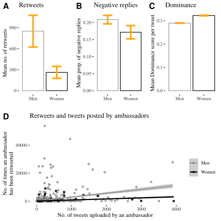
Figure 4.2: Retweets, negative replies, and dominance received by ambassadors. All four figures show descriptive means with 95% confidence intervals and without controls. Figure C shows the mean dominance score per tweet, while the remaining figures show the mean number of retweets and proportion of negative replies per ambassador.

We begin the analysis by testing Hypothesis 1, which predicts that women ambassadors are less visible online compared to their men colleagues. We find that this is indeed the case when measuring visibility as the number of retweets, as illustrated in the descriptive Fig 4.2 A. Women receive on average 406 fewer retweets ($p<0.05$) than men when excluding control variables. In other words, women receive on average 66.4% fewer retweets. The difference in visibility through retweets is persistent even when examining ambassadors who themselves are highly active on Twitter. This is illustrated in Fig 4.2 D. Here, each node represents an ambassador, the axes reflect the number of times an ambassador is retweeted and the number of original tweets uploaded by the ambassadors themselves.

It is important to note that 19.5% of women and 27.8% of all men in the sample received 0 retweets during the time period. While the exact reason for this is unknown, the lack of retweets likely reflects inactivity on Twitter. Ambassadors who have not been retweeted a single time post 16.4 times fewer original tweets (13.7 tweets on average) than those who have posted at least one tweet. Our estimations of gender bias are therefore conservative when considering that there are more inactive ambassador men with 0 retweets than women. In other words, men would have an even higher average than women if one removed all inactive accounts from the data.

The difference in visibility between men and women becomes smaller when including control variables, however, it remains substantial. Tab B1 in the Appendix shows the results based on a negative binomial regression model, in order to control for the sending countries (where the ambassadors are from) and receiving countries (where the ambassadors are assigned to). Using a multilevel framework, all of the ambassadors (i.e., observations) are nested either in their receiving country (Model 1, Model 3) or sending country (Model 2 and 4) with the countries serving as random effects in the models. Results in Model 1 in Tab B1 indicate that women ambassadors receive on average 45.7% fewer retweets than their men colleagues.This is the case when controlling for their receiving country, the number of tweets uploaded by the ambassador (n tweets) and the global prestige of the receiving country, measured as the standardized number of countries that send an embassy to the respective country (in-degree (receiving country)).

The gender difference is smaller when controlling for sending instead of the receiving countries (Model 2). Here, women receive 36.2% fewer retweets than men. In both cases, the difference is both statistically significant and substantively large. The findings are robust also when using a zero-inflated reiteration of the models as well as negative binomial models without the multilevel, nested data structure.

Estimates in Model 3 and 4 in Tab B1 indicate that women ambassadors have 16.5% or 17.5% fewer followers than men when controlling for the receiving country and sending country respectively. These results, however, are not robust. The difference is no longer statistically significant when using country-level fixed effects in the negative binomial models instead of nested, multilevel structure (see Appendix Tab B2).

Visibility and Prestige

We now turn to Hypothesis 1.1, which predicts that gender bias against women in terms of diminished visibility is more pronounced among ambassadors holding more prestigious positions. As previously mentioned, we analyze prestige by using standardized in-degree centrality, which measures the extent to which other nations establish embassies in the respective country. To examine this hypothesis, we employ a multilevel negative binomial regression model, where we control for the log number of tweets uploaded by the ambassador, the ambassador’s receiving country (Model 1, Model 3), and the sending country (Model 2 and 4). The regression tables are available in Appendix Tab D7.

Our estimates for differences in retweets support the hypothesis: Women sent to prestigious countries (with above-median in-degree score) receive on average 42.9% fewer retweets than women assigned to less prestigious destinations with up to median in-degree scores when controlling for the sending country. The difference is at 36.2% when controlling for the sending countries instead. In line with the results in the previous section, we observe no statistically significant difference when looking at the number of followers (Models 3 and 4 in Appendix Tab D7).

In other words, we observe an online glass ceiling effect when examining visibility through retweets. The relatively few women who gain prestigious, diplomatic positions in the men-dominated diplomatic sphere may experience an additional barrier at the top in the competition for online visibility.

4.7.2 Negativity in Replies

We now proceed to test Hypothesis 2, which predicts that women receive more negativity in public replies than men overall. We find no support for the hypothesis on a global level. This part of the analysis is limited to 1,424 ambassadors who have received at least one reply in the data. The descriptive Fig 4.2 B illustrates the proportion of negative replies sent to men and women. Contrary to the hypothesis, women receive on average 0.37 fewer percent points of negative replies, when running a simple OLS without controls, as shown in Model 1 in Appendix Tab B6. Although statistically significant ($p<0.01$), the difference is arguably too small to be substantively meaningful.

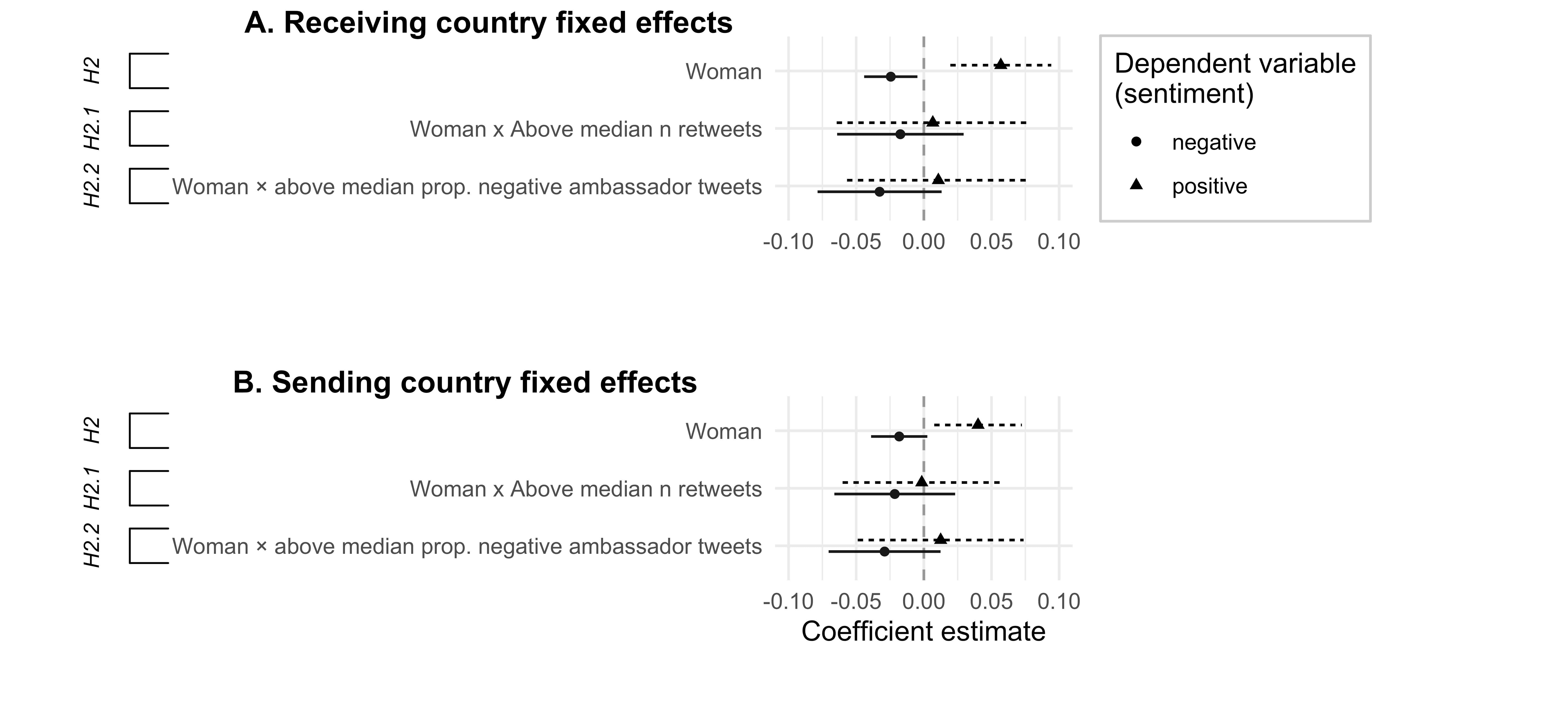
Figure 4.3: The difference in the proportion of negative and positive replies sent to the ambassadors. Figure A and Figure B show estimates with receiving and sending country fixed effects respectively. The brackets mark the relevant hypotheses corresponding to each row. For estimates with receiving country fixed effects (Figure A), the first row (H2) is based on Model 1, the second row (H2.1) is based on Model 2, and the third row is based on Model 3 (H2.2). For estimates with sending country fixed effects (Figure B), the estimates are based on models 4, 5, and 6 in the respective order. All of the models are available in Appendix Tab B3 and Tab B4.

The first row in Fig 4.3 shows the difference in proportion of negative replies between men and women when controlling for number of tweets uploaded by the ambassadors, the in-degree of the receiving country, a dummy variable for whether the ambassadors receive above median number of retweets as well as countries through receiving country fixed effects (Model 1, Appendix Tab B3) and sending country fixed effects (Model 4, Appendix Tab B3). While the overall pattern is the same, the difference in the proportion of negativity in replies is even smaller in models with controls. Women receive on average from 0.018 to 0.25 percent points less negativity than men, depending on the model specification. The difference is no longer statistically significant when adding a binary control variable for whether the ambassadors themselves post above the median proportion of negative tweets or not (Model 3 and 6 in Appendix Tab B3).

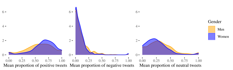
Figure A4: Sentiment in tweets posted by ambassadors (density plots)

We validate the analysis by reiterating the models above with the proportion of positive replies as the dependent variable. The results point in the same direction. Women receive on average 6.1 percent points higher proportion of positive replies than men when running a simple OLS without controls ($p<0.01$). The pattern holds when including the control variables, as illustrated in Fig 4.3. Here, the difference ranges from 4.5 to 5.6 percent points (Model 1 and 4 in Appendix Tab B4). This is not surprising when taking into account that women post fewer negative tweets themselves (see Appendix Fig A4 and Tab A1) and that negative ambassador tweets are associated with a lower proportion of positive tone in the replies in our data. The difference between men and women ambassadors is no longer statistically significant when controlling for the proportion of negative tweets posted by the ambassadors and their country of origin through sending-country fixed effects.

Is the correlation between gender and tone in the replies mitigated by the visibility or tone in the original tweets posted by the ambassadors themselves? We investigate this by testing Hypotheses 2.1 and 2.2.

Negativity and Visibility

Hypothesis 2.1 predicts that the gender bias against women is stronger among ambassadors with high visibility, while Hypothesis 2.2 predicts that the bias increases among ambassadors who write more negative tweets themselves. In the case of Hypothesis H2.1, we would expect a positive interaction between gender and the number of retweets received by the ambassador, denoted by Woman $\times$ Above median n retweets, when examining the proportion of negative tweets as the dependent variable. In other words, women with many retweets would receive more negativity than those with less visibility. Contrary to the hypothesis, the interaction term is negative, statistically insignificant as well as both substantively small as shown in Fig 4.3 and Appendix Tab B3, when controlling for number of original ambassador tweets, receiving country in-degree and retweets.

Negativity and Self-Negativity

In cases of Hypothesis 2.2, we would observe a positive interaction term for: Woman $\times$ above median prop. negative ambassador tweets, in the same figure and table. To put it differently, we would expect that women who go against the gender-stereotypical role by posting a higher proportion of negative tweets themselves would receive more negativity than women, who post fewer negative tweets. As shown in Fig 4.3 and Appendix Tab B3, our results do not support this hypothesis: the interaction term is negative, substantively small, and statistically insignificant when using the same control variables as above.

In addition, we find no evidence for Hypotheses 2.1. and 2.2 when replacing the dependent variable with the proportion of positive replies in the validation step (see Fig 4.3). The results remain robust despite different model specifications: when using receiving country fixed effects, sending country fixed effects ( Appendix Tab B3 and Tab B4), simple OLS only with variables of interest (Appendix Tab B6). In sum, our data does not indicate that women receive more negative, public replies on a global level or that the potential gender bias through negative sentiment is mediated through visibility or the sentiment in the original ambassador tweets.

4.7.3 Gendered Language

We now turn to examining whether women ambassadors are targeted with gendered language, as predicted by Hypothesis 3. In the first part of this section, we will examine the levels of dominance in the replies sent to the ambassadors. In the second part of the section, we will proceed to a more qualitative interpretation of the words associated with replies sent to men and women.

4.7.3.1 Dominant Language

This part of the analysis is based on the 1,367 ambassadors that have received at least one reply with a classified dominance score. The descriptive distribution is illustrated in Fig 4.2 C. The mean dominance score in replies sent to women is 0.013 higher compared to replies sent to men ($p<0.01$) when running an OLS model with no controls. The mean dominance score is 0.331 for men and 0.344 for women. The average dominance score is 3.9% higher in replies sent to women than the average dominance score in the replies sent to men according to these estimates.

As shown in Appendix Tab B5, the average dominance score in replies sent to women ranges from 0.010 to 0.012 higher than that sent to men – depending on the model specification. The difference remains statistically significant even when controlling for the number of ambassador tweets, visibility through retweets, the prestige of the country that the ambassadors are assigned to (measured as in-degree), and the receiving or sending country through fixed effects. In other words, the average level of dominance in the replies sent to women is at least 3.1% higher than the levels of dominance sent to men – according to the most conservative estimate, when including the controls. In an additional analysis outside of this section, we find no evidence suggesting that women with higher visibility (measured as retweets) receive more dominance in replies than women with fewer retweets. The same pattern holds when comparing women with above median proportion of negative original ambassador tweets with women who post fewer negative tweets.

Overall, our analysis shows that the language used by Twitter users who reply to women and men ambassadors is indeed gendered in line with Hypothesis 3. The difference is not high, but it is important when considering that ambassadors collectively are responded to by millions of tweets throughout multiple years. Notably, the global difference is persistent when incorporating approximately 65 languages sent to 1,367 ambassadors from a total of 148 countries.

4.7.3.2 Lexical Biases

In this section, we investigate the lexical differences in responses to men and women ambassadors. To this end, we analyze word usage towards ambassadors being received by countries with the highest number of tweets in response. The top 10 women- and men-associated words identified using $\mathrm{PMI}$ for the top 5 countries receiving ambassadors with the highest number of responses are shown in Tab 4.2.

Receiving country	Associated words
Men-biased
India	sir, support, Israel, love, friend, students, open, India, visa, decision
Brazil	China, party, Brazil, people, thank, help, way, country, years, respect
United States	Tigray, tigraygenocide, Ethiopia, Chinese, lie, ethnic, Ethiopian, Irish,
	rape, independent
Lebanon	Mr, Saudi, government, new, come, send, times, company, appreciate
	big
Iraq	Iraq, amp, militias, hope, time, UK, Iraqi, government, people, country
Women-biased
India	Finland, Finnish, engage, software, actively, cheated, flowers, owners
	heargaza, plus
Brazil	happy, culture, brain, time, technology, terrorism, want, know
	ministers, best
United States	Saudi, salmon, mbs, saudiarabia, highness, Arabia, colored, prince
	Arab, queens
Lebanon	teachers, quality, general, UNRWA, decision, Australian, jobs, Gaza
	paid, learn
Iraq	president, bless, Jordan, national, office, interesting, kdp, missions
	official, asking

Table 4.2: The top-10 men (top) and women-biased (bottom) words in the dataset for the top-5 receiving countries with the highest numbers of tweets written in response to the ambassadors, using $\mathrm{PMI}$.

We observe that the words written in response to ambassadors whether men or women cover predominantly international politics and diplomacy. We verify this by employing Latent Dirichlet analysis (LDA; Blei2003LDA) on the subset of tweets in English written in response to the ambassadors. We find that indeed the topics covered evolve to a high degree around politics and diplomacy (see Tab C1 in the Appendix). Additional validation of both results related to negativity and gendered language is available in the Validation section in Appendix C.

4.8 Conclusion

Historically, diplomacy has been a men-dominated field, with women facing various forms of discrimination and bias. While there have been changes, gender inequalities persist in the diplomatic profession. This study’s focus on social media, specifically Twitter, is significant as Twitter has become the platform of choice for diplomats worldwide, making it a critical space for shaping international discourse.

Our findings challenge common assumptions about online gender bias against women. Contrary to expectations, women ambassadors do not face a higher degree of outright negativity in responses to their tweets on a global scale. Although they do receive more gendered language in the replies, the difference is not substantively large. Instead, the primary source of online bias against women ambassadors is their lower online visibility. This subtler form of bias, while less overt, is of paramount importance, as it affects their ability to engage in public diplomacy effectively. We also observe an interesting online glass-ceiling effect: The relatively few women who gain prestigious, diplomatic positions in the men-dominated diplomatic sphere experience an additional barrier at the top in the competition for online visibility. The implications of these findings are twofold. On one hand, the diplomatic arena may provide a relatively ‘safer’ online space for women compared to other political domains. On the other hand, it underscores the deeply ingrained nature of these biases, including the value attached to tweets by women ambassadors compared to their men colleagues.

By conducting the first global-scale, systematic study of gender bias in digital diplomacy, the research not only sheds light on the multifaceted nature of online gender bias but also provides essential methodological insights for future investigations and a foundation for cross-temporal and cross-platform comparisons. Our findings illustrate the methodological importance of combining analysis of publicly available content with a more network-centered analysis of retweets. While gender bias may appear small in the publicly available content, one risks overlooking inequality in a more latent, yet highly important resource, online visibility itself. The findings illuminate subtle biases in interactions between ambassadors and their audiences, leaving a more detailed analysis of how ambassadors interact with other ambassadors outside of the scope of this study.

Our research not only advances our understanding of gender bias in digital diplomacy but also contributes to the broader conversation on gender equality in international politics. It underscores the importance of exploring how to ensure greater online visibility for women ambassadors, as this visibility is not just a matter of representation but also a fundamental resource for engaging in diplomatic activities on social media. As such, this study provides a critical foundation for future research and policy development aimed at reducing gender bias in the realm of digital diplomacy and beyond.

The study is limited to Twitter, which is the main home of digital diplomacy even today. However, gender bias patterns may be different when looking at other social media, and perhaps even the future versions of the same platform. Social media platforms constantly change due to updated algorithms, moderation policies, and functions. As “Twitter” has transitioned into “X”, the information environment on Twitter is changing, potentially also the gender bias we observe.

Lastly, the study does not measure how gender interacts with other biases related to the ambassadors’ ethnicity, perceived race, religion, or other factors. We hope that our multilingual and globally-spanning study will serve as a stepping stone for future research on intersectionality in digital diplomacy.

Funding: Research for this paper has been funded by the European Research Council as part of the StG DIPLOFACE 680102 and “Independent Research Fund Denmark under grant agreement number 9130-00092B”.

4.9 Appendix

Appendix A: Descriptive Statistics

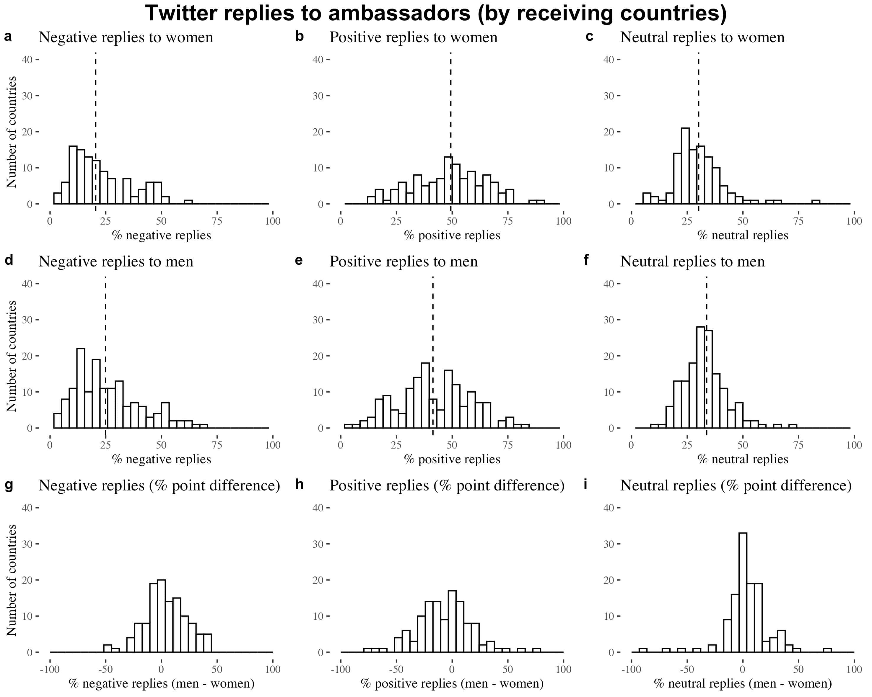
Figure A1: The figure shows the aggregated distribution of negative, positive and neutral replies sent to ambassadors in their destination countries. Vertical lines reflect means. Values in the lowest row reflect the difference between the mean proportion of sentiment (positive, negative or neutral) for men minus the mean proportion for women.

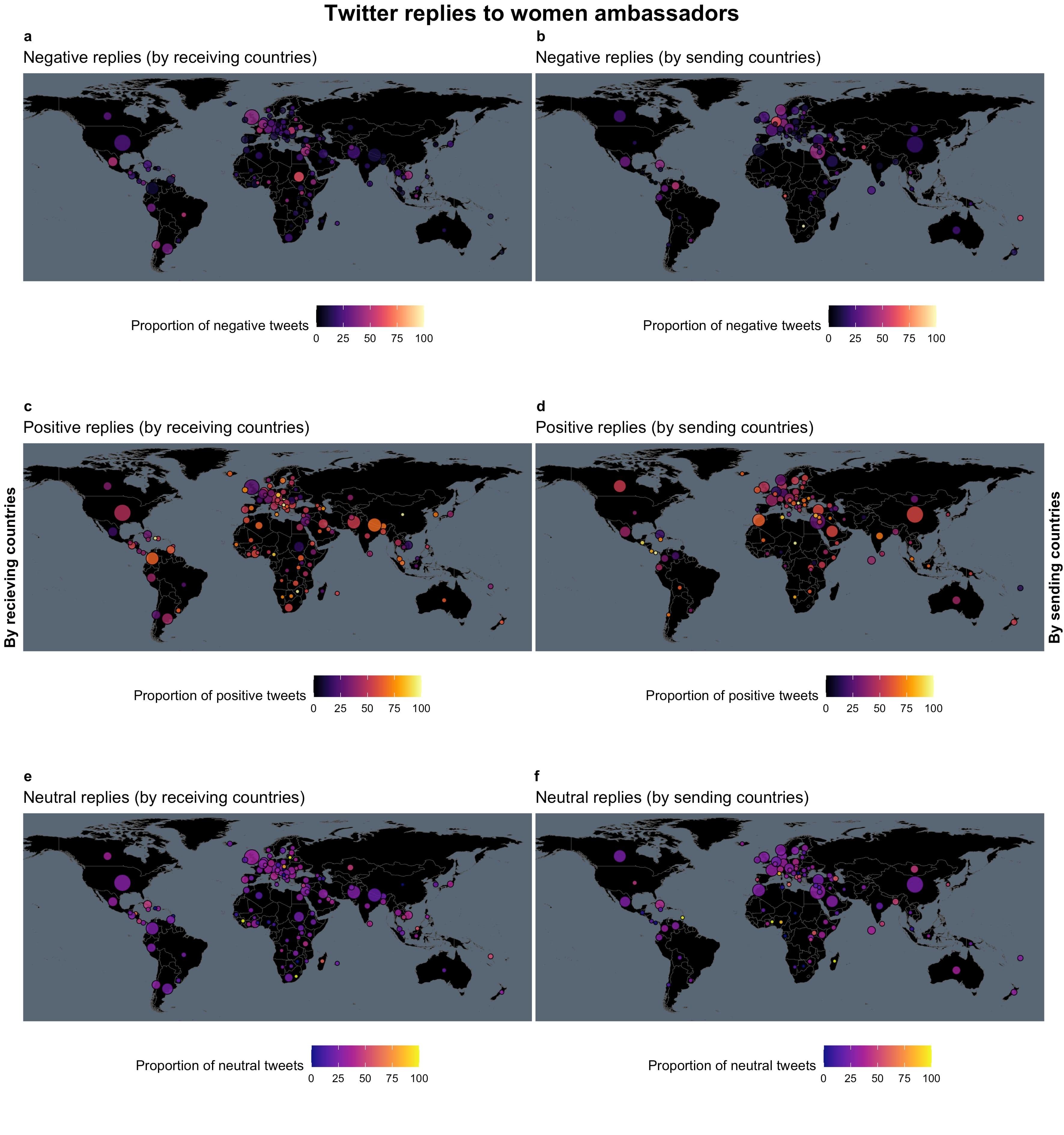
Figure A2: Node size reflects the number of replies. Columns to the left reflect values for ambassadors who are sent to respective destinations, while columns to the right reflect values for ambassadors originating from the given countries.

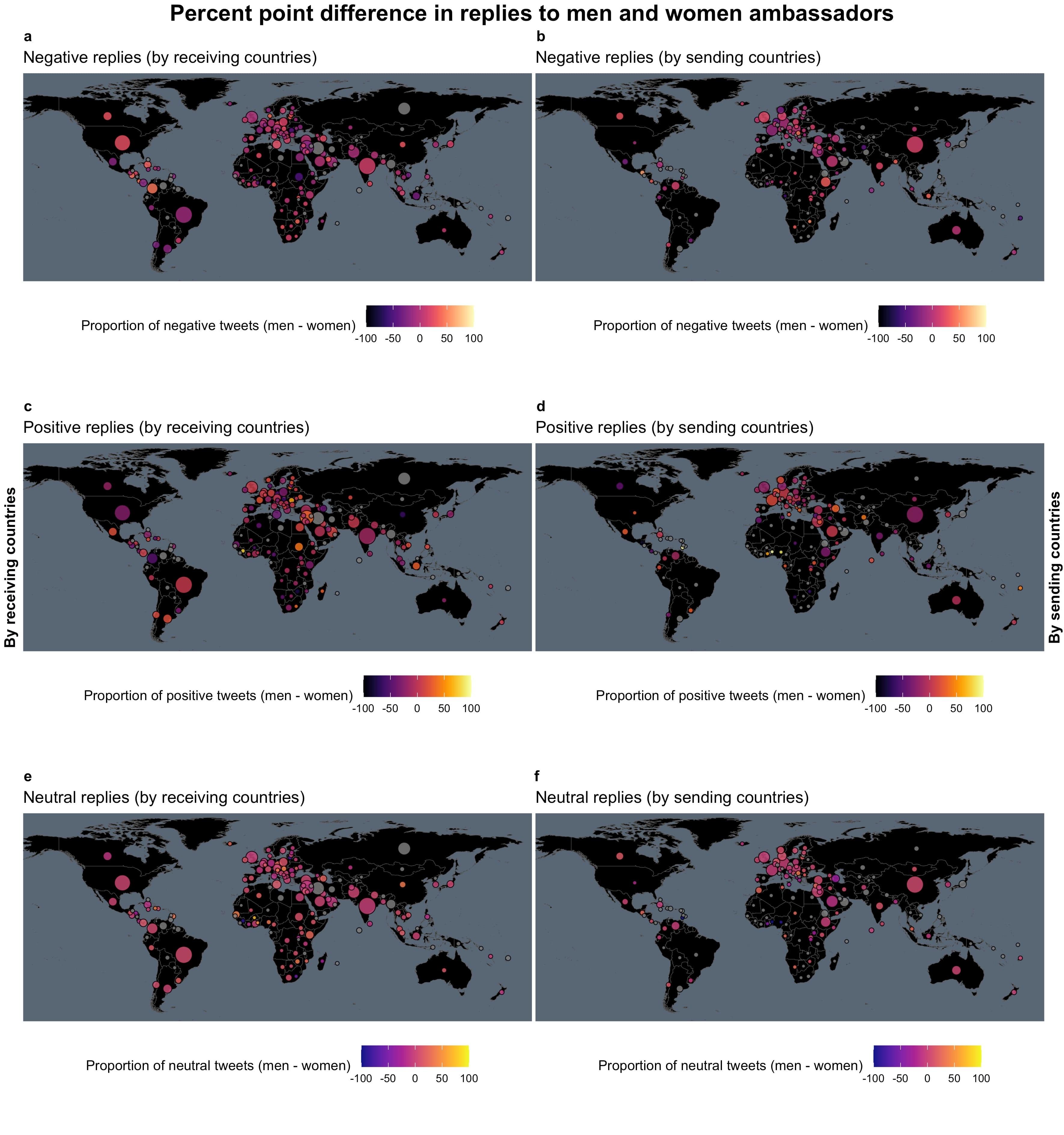
Figure A3: Node size reflects the number of replies. Grey color indicates that there are only men in the subsample. Color reflects the difference between the mean proportion of sentiment (positive, negative, or neutral) for men minus women. For example, lower (darker) values in Figure a indicate that women ambassadors on average receive a higher proportion of negative replies than their men colleagues who are sent to the respective country.

Figure A5: Valence, arousal, and dominance scores in tweets posted by ambassadors (density plots)

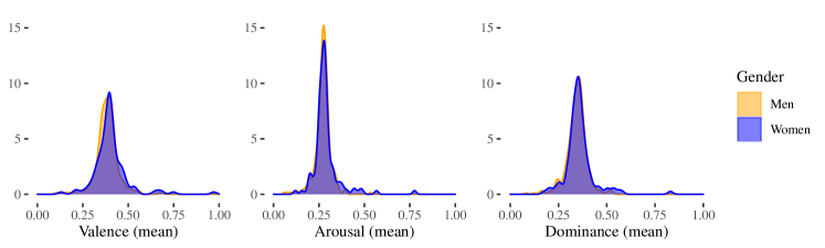
Figure A6: Mean valence, arousal, and dominance scores (for each ambassador) in tweets posted by ambassadors (density plots)

Table A1: Descriptive overview of sentiment, valence, arousal, and dominance scores in tweets posted by ambassadors

	Men	Women
Total number of tweets	104,531	37,012
Mean tweets	91.94	78.58
SD tweets	150.45	153.00
Median tweets	42	39
Mean % of positive tweets	0.58	0.65
SD % of positive tweets	0.25	0.23
Mean % of negative tweets	0.10	0.09
SD % of negative tweets	0.14	0.13
Mean % of neutral tweets	0.32	0.26
SD % of neutral tweets	0.23	0.20
Mean Valence	0.36	0.38
SD Valence	0.12	0.13
Mean Arousal	0.26	0.27
SD Arousal	0.08	0.09
Mean Dominance	0.33	0.33
SD Dominance	0.10	0.10

Appendix B: Regression Models

Table B1: Negative Binomial Multilevel models: Estimating difference in visibility measured as retweet and follower count. Ambassadors are nested in their respective receiving countries (Models 1 and 3) and sending countries (Models 2 and 4). The coefficients reflect log change in the dependent variables per unit change in the independent variables.

	Dependent variables:
	Retweets		Followers
	Model 1	Model 2	Model 3	Model 4
Intercept	$-0.90^{***}$	$-1.20^{***}$	$6.26^{***}$	$5.73^{***}$
	$(0.20)$	$(0.18)$	$(0.16)$	$(0.14)$
in-degree (receiving country)	$1.65^{***}$	$1.16^{***}$	$1.60^{***}$	$1.66^{***}$
	$(0.42)$	$(0.18)$	$(0.37)$	$(0.15)$
Woman	$-0.61^{***}$	$-0.45^{***}$	$-0.18^{*}$	$-0.19^{*}$
	$(0.10)$	$(0.09)$	$(0.08)$	$(0.08)$
log(n tweets + 0.1)	$1.17^{***}$	$1.17^{***}$	$0.36^{***}$	$0.31^{***}$
	$(0.02)$	$(0.03)$	$(0.01)$	$(0.01)$
AIC	$18636.63$	$18333.98$	$34977.08$	$34599.22$
Log Likelihood	$-9312.31$	$-9160.99$	$-17482.54$	$-17293.61$
Num. obs.	$1960$	$1960$	$1948$	$1948$
Num. groups: Receiving country	$172$		$172$
Var: Receiving country (Intercept)	$0.90$		$0.70$
Num. groups: Sending country		$164$		$163$
Var: Sending country (Intercept)		$1.41$		$1.50$
${}^{***}p<0.001$; ${}^{**}p<0.01$; ${}^{*}p<0.05$

Table B2: Negative Binomial models with country-level fixed effects: Estimating difference in visibility measured as retweet and follower count

Dependent Variables:	Retweets		Followers
Model:	(1)	(2)	(3)	(4)
Variables
Woman	-0.4022∗∗∗	-0.5538∗∗∗	-0.1732	-0.1201
	(0.1341)	(0.1348)	(0.1141)	(0.1223)
log(n tweets+0.1)	1.155∗∗∗	1.199∗∗∗	0.3018∗∗∗	0.3694∗∗∗
	(0.0423)	(0.0687)	(0.0269)	(0.0277)
in-degree (receiving country)	1.213∗∗∗		1.711∗∗∗
	(0.3272)		(0.2338)
Fixed-effects
Sending country	Yes		Yes
Receiving country		Yes		Yes
Fit statistics
Standard-Errors	Sending	Receiving	Sending	Receiving
Squared Correlation	0.13338	0.10530	0.14987	0.09290
BIC	19,003.7	19,518.6	35,362.8	35,883.9
Over-dispersion	0.50944	0.44309	0.59918	0.50779
Signif. Codes: ***: 0.01, **: 0.05, *: 0.1

Table B3: OLS with country-level fixed effects: The difference in proportion of negative replies sent to the ambassadors

Dependent Variable:	Proportion of negative replies
Model:	(1)	(2)	(3)	(4)	(5)	(6)
Variables
Woman	-0.0244∗∗	-0.0163	-0.0030	-0.0182∗	-0.0079	0.0007
	(0.0100)	(0.0171)	(0.0143)	(0.0106)	(0.0174)	(0.0154)
log(n tweets +0.1)	-0.0014	-0.0015	-0.0086∗	-0.0064	-0.0066	-0.0121∗∗
	(0.0049)	(0.0049)	(0.0047)	(0.0055)	(0.0055)	(0.0056)
Above median n retweets	0.0785∗∗∗	0.0834∗∗∗	0.0837∗∗∗	0.0503∗∗∗	0.0569∗∗∗	0.0559∗∗∗
	(0.0115)	(0.0147)	(0.0114)	(0.0163)	(0.0161)	(0.0157)
Woman $\times$		-0.0174			-0.0215
Above median n retweets		(0.0239)			(0.0228)
Above median prop. negative			0.0932∗∗∗			0.0930∗∗∗
ambassador tweets			(0.0122)			(0.0110)
Woman $\times$ Above median			-0.0327			-0.0290
prop. negative ambassador			(0.0234)			(0.0211)
tweets
in-degree (receiving)				0.0667∗∗∗	0.0668∗∗∗	0.0717∗∗∗
				(0.0225)	(0.0225)	(0.0221)
Fixed-effects
Receiving country	Yes	Yes	Yes
Sending country				Yes	Yes	Yes
Fit statistics
Standard-Errors	Receiving	Receiving	Receiving	Sending	Sending	Sending
Observations	1,424	1,424	1,424	1,424	1,424	1,424
Signif. Codes: ***: 0.01, **: 0.05, *: 0.1

Table B4: OLS with country-level fixed effects: The difference in the proportion of positive replies sent to the ambassadors

Dependent Variable:	Proportion of positive replies
Model:	(1)	(2)	(3)	(4)	(5)	(6)
Variables
Woman	0.0569∗∗∗	0.0538∗	0.0457∗	0.0401∗∗	0.0408	0.0305
	(0.0190)	(0.0313)	(0.0248)	(0.0165)	(0.0273)	(0.0222)
log(n tweets +0.1)	0.0221∗∗∗	0.0222∗∗∗	0.0297∗∗∗	0.0286∗∗∗	0.0286∗∗∗	0.0326∗∗∗
	(0.0057)	(0.0057)	(0.0057)	(0.0054)	(0.0054)	(0.0053)
Above median n retweets	-0.0596∗∗∗	-0.0614∗∗∗	-0.0654∗∗∗	-0.0243	-0.0238	-0.0283
	(0.0174)	(0.0209)	(0.0175)	(0.0198)	(0.0213)	(0.0196)
Woman $\times$ Above median		0.0066			-0.0015
n retweets		(0.0363)			(0.0299)
Above median prop. neg.			-0.0925∗∗∗			-0.0645∗∗∗
tweets			(0.0163)			(0.0196)
Woman $\times$ Above median			0.0107			0.0124
prop. neg. tweets			(0.0344)			(0.0313)
in-degree (receiving)				-0.0378	-0.0378	-0.0409
				(0.0298)	(0.0298)	(0.0302)
Fixed-effects
Receiving country	Yes	Yes	Yes
Sending country				Yes	Yes	Yes
Fit statistics
Standard-Errors	Receiving	Receiving	Receiving	Sending	Sending	Sending
Observations	1,424	1,424	1,424	1,424	1,424	1,424
Signif. Codes: ***: 0.01, **: 0.05, *: 0.1

Table B5: OLS with country-level fixed effects: The difference in average dominance scores in replies sent to the ambassadors

Dependent Variable:	Mean Dominance score
Model:	(1)	(2)	(3)	(4)
Variables
Woman	0.0116∗∗∗	0.0110∗∗∗	0.0101∗∗∗	0.0102∗∗∗
	(0.0038)	(0.0036)	(0.0038)	(0.0036)
log(n tweets +0.1)			0.0031∗∗	0.0037∗∗
			(0.0014)	(0.0014)
Above median n retweets			-0.0178∗∗∗	-0.0079
			(0.0053)	(0.0050)
in-degree (receiving)				-0.0228∗∗∗
				(0.0079)
Fixed-effects
Receiving country	Yes		Yes
Sending country		Yes		Yes
Fit statistics
Standard-Errors	Receiving	Sending	Receiving	Sending
Observations	1,367	1,367	1,367	1,367
Signif. Codes: ***: 0.01, **: 0.05, *: 0.1

Table B6: Simple OLS only with variables of interest: The difference in the proportion of negative and positive replies sent to the ambassadors

	Dependent variable:
	Proportion of negative replies			Proportion of positive replies
	(1)	(2)	(3)	(4)	(5)	(6)
Woman	$-$0.037∗∗∗	$-$0.020	$-$0.014	0.061∗∗∗	0.060∗∗∗	0.049∗∗
	(0.012)	(0.016)	(0.016)	(0.016)	(0.022)	(0.023)
Above median n retweets		0.077∗∗∗			$-$0.005
		(0.013)			(0.018)
Woman $\times$ above median		$-$0.025			0.001
n retweets		(0.024)			(0.033)
Above median prop. neg.			0.104∗∗∗			$-$0.071∗∗∗
tweets			(0.012)			(0.017)
Woman $\times$ above median			$-$0.037			0.017
prop. neg. tweets			(0.023)			(0.033)
Constant	0.209∗∗∗	0.168∗∗∗	0.155∗∗∗	0.436∗∗∗	0.439∗∗∗	0.473∗∗∗
	(0.006)	(0.009)	(0.009)	(0.009)	(0.013)	(0.013)
Observations	1,424	1,424	1,424	1,424	1,424	1,424
R2	0.007	0.037	0.061	0.010	0.010	0.024
Adjusted R2	0.006	0.035	0.059	0.009	0.008	0.021
Note:	∗p$<$0.1; ∗∗p$<$0.05; ∗∗∗p$<$0.01

Appendix C: Validation

We validate the results through three steps. In the first step, we validate the findings on negativity by detecting incivility in direct replies sent to ambassadors in English. For this purpose, we use a machine-learning-based incivility algorithm originally developed by theocharis_dynamics_2020 for their study of tweets sent to US members of Congress. The score ranges from 0 (civil) to 1 (uncivil). We find that women receive on average slightly more civil tweets than their men colleagues. This further corroborates the results based on sentiment, which indicate that women do not receive more negatively than men overall. The density plot below gives a descriptive overview of the distribution of the incivility score (Fig C1).

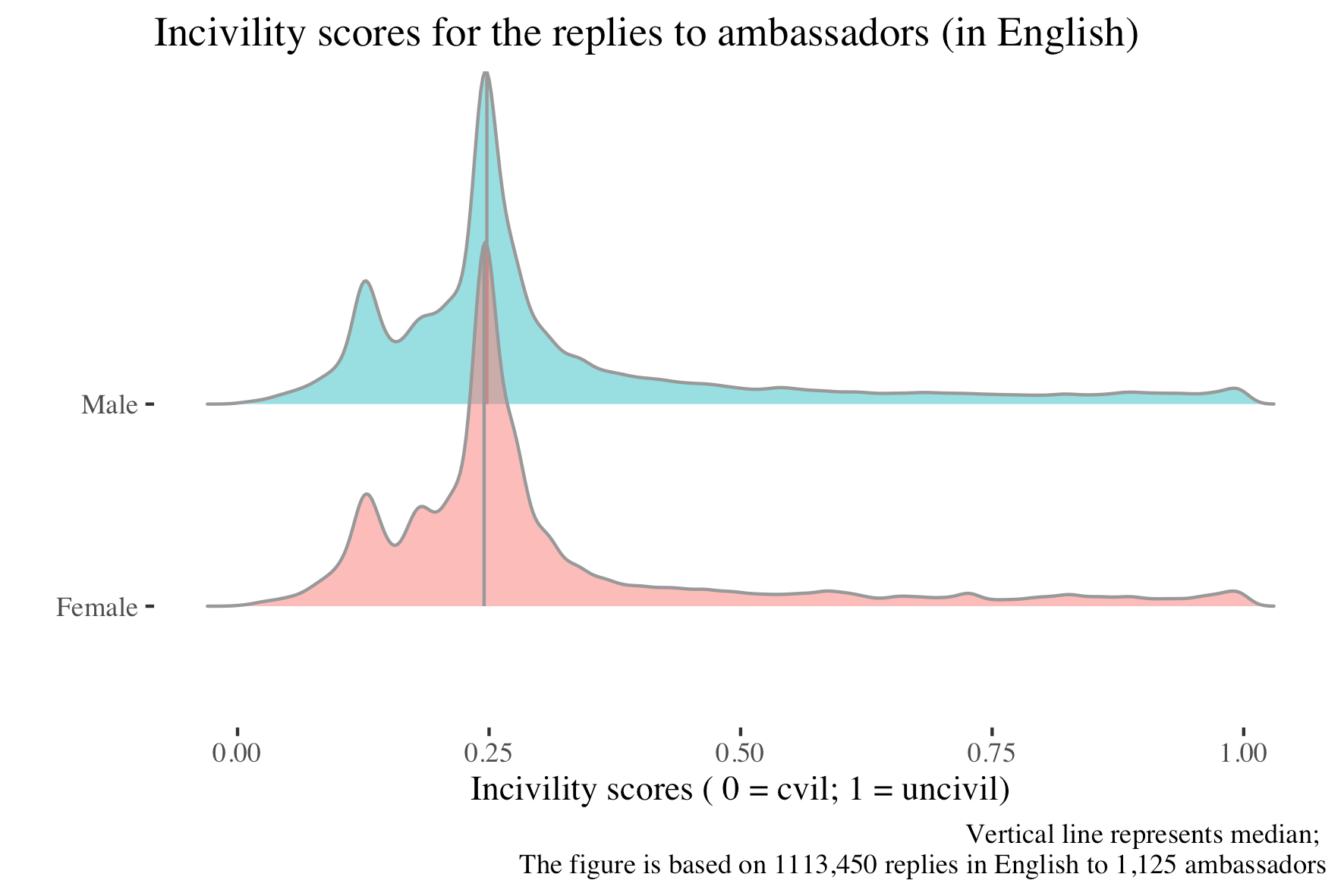
Figure C1:

In the second step, we verify that replies sent to women ambassadors are mainly related to political topics by using Latent Dirichlet analysis (LDA; Blei2003LDA) to identify topics in direct replies sent to ambassadors in English. We find that indeed the topics covered evolve to a high degree around politics and diplomacy (see Tab C1 in the Appendix).

Topic	Associated words
Topic 1	China, annlinde, Tigray, world, Chinese, people, time, act, EU, take
Topic 2	annlinde, Pakistan, country, Canada, world, people, women, one, see, like
Topic 3	Israel, people, children, terrorist, crimes, Israeli, Palestinian, state, Palestine
Topic 4	you, women, …, marisepayne, what, Australia, n’t, like, get
Topic 5	Myanmar, military, please, people, junta, election, respect, ASEAN
	whatshappeninginmyanmar, coup
Topic 6	human, happy, rights, annlinde, you, new, this, day, peak, please
Topic 7	thank, thanks, great, help, good, much, ambassador, excellency, congratulations
Topic 8	want, respect, government, !!!, need, !!, leader, votes, another, please
Topic 9	not, minister, foreign, meet, please, people, n’t, represent, Myanmar, Thailand

Table C1: The top-9 identified topics based on all tweets written in English in response to the ambassadors.

In the last step, we examine whether gender bias through retweets, negativity and dominance in replies is mediated by the overall levels of gender inequality in the respective countries. To ensure robustness, we operationalize country-level gender inequality using three, established measures: 1) Gender Inequality Index (GII_2020; QOG_2022), Proportion of seats held by women in national parliaments (World_Bank2021; QOG_2022) and Gender Social Norms Index (GSNI_2020) with the latest observations as of 2019. These results as shown in the regression tables in Appendix D. The overall finding remains the same: We find a strong gender bias in visibility through retweets even when taking into account gender inequality in the sending or receiving country. In addition to this, we find no evidence that women receive fewer retweets, more negativity or dominant language in replies if they originate from- or are sent to countries with above-median levels of gender inequality. We observe one exception: Women who are sent to a country with a high Gender Social Norms Index receive slightly more dominant replies, however, the difference is not substantial.

Appendix D: Gender Inequality in Sending and Receiving Countries

This appendix presents additional robustness checks. Models in Tables D1 to D6 test whether the difference in visibility between men and women is mediated by levels of gender inequality in the respective countries. The latter is operationalized as 1) Gender Inequality Index, 2) Proportion of women in parliament and 3) Gender Social Norms Index. The respective models take into account either the gender inequality in the sending country, i.e., an ambassador’s country of origin, or the receiving country that the ambassador is assigned to. The number of observations varies because it is not possible to obtain the same inequality measurements for all countries. Models in Table D7 test whether the difference in visibility is mediated by the prestige of the receiving country, measured as that country’s in-degree in a diplomatic network, where each tie reflects one country sending an embassy to another country. Models in Table D8 test whether negativity is mediated by either prestige (in-degree), Gender Inequality Index or proportion of women in parliament in the receiving country.

Table D1: Negative Binomial Multilevel models: Gender Inequality Index in receiving countries and visibility. Estimating difference in visibility measured as retweet and follower count. Ambassadors are nested in their respective receiving countries (Models 1 and 3) and sending countries (Models 2 and 4). The coefficients reflect log change in the dependent variables per unit change in the independent variables.

Dependent Variables:	Retweets		Followers
Model:	(1)	(2)	(3)	(4)
Intercept	$-1.73^{***}$	$-1.87^{***}$	$5.80^{***}$	$5.50^{***}$
	$(0.27)$	$(0.20)$	$(0.23)$	$(0.16)$
in-degree (receiving country)	$2.53^{***}$	$1.70^{***}$	$1.96^{***}$	$1.85^{***}$
	$(0.42)$	$(0.19)$	$(0.40)$	$(0.16)$
Woman	$-0.62^{***}$	$-0.36^{**}$	$-0.06$	$-0.16$
	$(0.14)$	$(0.12)$	$(0.12)$	$(0.11)$
Gender Inequality Index	$0.73^{***}$	$0.63^{***}$	$0.56^{**}$	$0.29^{**}$
	$(0.20)$	$(0.10)$	$(0.19)$	$(0.09)$
log(n tweets + 0.1)	$1.18^{***}$	$1.19^{***}$	$0.36^{***}$	$0.31^{***}$
	$(0.02)$	$(0.03)$	$(0.01)$	$(0.01)$
Woman x Gender Inequality Index	$0.04$	$-0.02$	$-0.32$	$-0.02$
	$(0.20)$	$(0.17)$	$(0.17)$	$(0.15)$
AIC	$18185.44$	$17853.24$	$34087.11$	$33705.72$
Log Likelihood	$-9084.72$	$-8918.62$	$-17035.55$	$-16844.86$
Num. obs.	$1907$	$1907$	$1895$	$1895$
Num. groups: Receiving country	$156$		$156$
Var: Receiving country (Intercept)	$0.69$		$0.65$
Num. groups: Sending country		$163$		$162$
Var: Sending country (Intercept)		$1.35$		$1.49$
${}^{***}p<0.001$; ${}^{**}p<0.01$; ${}^{*}p<0.05$

Table D2: Negative Binomial Multilevel models: Gender Inequality Index in sending countries and visibility. Estimating difference in visibility measured as retweet and follower count. Ambassadors are nested in their respective receiving countries (Models 1 and 3) and sending countries (Models 2 and 4). The coefficients reflect log change in the dependent variables per unit change in the independent variables.

Dependent Variables:	Retweets		Followers
Model:	(1)	(2)	(3)	(4)
Intercept	$-0.67^{**}$	$-0.80^{**}$	$6.15^{***}$	$5.77^{***}$
	$(0.21)$	$(0.25)$	$(0.16)$	$(0.24)$
in-degree (receiving country)	$1.50^{***}$	$1.19^{***}$	$1.54^{***}$	$1.71^{***}$
	$(0.41)$	$(0.18)$	$(0.36)$	$(0.15)$
Woman	$-0.85^{***}$	$-0.72^{***}$	$-0.23^{*}$	$-0.32^{**}$
	$(0.13)$	$(0.12)$	$(0.11)$	$(0.10)$
Gender Inequality Index	$-0.30^{**}$	$-0.63^{*}$	$0.23^{*}$	$-0.09$
	$(0.11)$	$(0.26)$	$(0.09)$	$(0.27)$
log(n tweets + 0.1)	$1.16^{***}$	$1.16^{***}$	$0.36^{***}$	$0.31^{***}$
	$(0.02)$	$(0.03)$	$(0.01)$	$(0.01)$
Woman x Gender Inequality Index	$0.60^{**}$	$0.64^{***}$	$0.14$	$0.31$
	$(0.20)$	$(0.19)$	$(0.17)$	$(0.16)$
AIC	$18282.18$	$18020.81$	$34164.88$	$33809.45$
Log Likelihood	$-9133.09$	$-9002.41$	$-17074.44$	$-16896.72$
Num. obs.	$1912$	$1912$	$1900$	$1900$
Num. groups: Receiving country	$172$		$172$
Var: Receiving country (Intercept)	$0.87$		$0.67$
Num. groups: Sending country		$145$		$144$
Var: Sending country (Intercept)		$1.29$		$1.50$
${}^{***}p<0.001$; ${}^{**}p<0.01$; ${}^{*}p<0.05$

Table D3: Negative Binomial models: Visibility (retweet and follower count) and % of women in parliament in receiving country. Ambassadors are nested in their respective receiving countries (Models 1 and 3) and sending countries (Models 2 and 4). The coefficients reflect log change in the dependent variables per unit change in the independent variables.

Dependent Variables:	Retweets		Followers
Model:	(1)	(2)	(3)	(4)
Intercept	$-0.77^{***}$	$-0.92^{***}$	$6.29^{***}$	$5.81^{***}$
	$(0.22)$	$(0.19)$	$(0.17)$	$(0.15)$
in-degree (receiving country)	$1.70^{***}$	$1.19^{***}$	$1.60^{***}$	$1.67^{***}$
	$(0.42)$	$(0.18)$	$(0.37)$	$(0.15)$
Woman	$-0.73^{***}$	$-0.59^{***}$	$-0.35^{**}$	$-0.23^{*}$
	$(0.14)$	$(0.13)$	$(0.12)$	$(0.11)$
% of women in parliament	$-0.28$	$-0.51^{***}$	$-0.07$	$-0.16$
	$(0.19)$	$(0.10)$	$(0.17)$	$(0.08)$
log(n tweets + 0.1)	$1.17^{***}$	$1.15^{***}$	$0.36^{***}$	$0.31^{***}$
	$(0.02)$	$(0.02)$	$(0.01)$	$(0.01)$
Woman x % of women in parliament	$0.24$	$0.32$	$0.29$	$0.08$
	$(0.20)$	$(0.17)$	$(0.17)$	$(0.15)$
AIC	$18564.57$	$18235.23$	$34858.63$	$34481.58$
Log Likelihood	$-9274.29$	$-9109.62$	$-17421.32$	$-17232.79$
Num. obs.	$1954$	$1954$	$1942$	$1942$
Num. groups: Receiving country	$171$		$171$
Var: Receiving country (Intercept)	$0.88$		$0.70$
Num. groups: Sending country		$164$		$163$
Var: Sending country (Intercept)		$1.38$		$1.49$
${}^{***}p<0.001$; ${}^{**}p<0.01$; ${}^{*}p<0.05$

Table D4: Negative Binomial Multilevel Models: Visibility (retweet and follower count) and % of women in parliament in sending country. Ambassadors are nested in their respective receiving countries (Models 1 and 3) and sending countries (Models 2 and 4). The coefficients reflect log change in the dependent variables per unit change in the independent variables.

Dependent Variables:	Retweets		Followers
Model:	(1)	(2)	(3)	(4)
Intercept	$-0.83^{***}$	$-1.30^{***}$	$6.35^{***}$	$5.70^{***}$
	$(0.21)$	$(0.20)$	$(0.16)$	$(0.17)$
in-degree (receiving country)	$1.58^{***}$	$1.18^{***}$	$1.55^{***}$	$1.66^{***}$
	$(0.42)$	$(0.18)$	$(0.37)$	$(0.15)$
Woman	$-0.43^{**}$	$-0.07$	$-0.06$	$-0.14$
	$(0.15)$	$(0.14)$	$(0.12)$	$(0.12)$
Gender Inequality Index	$-0.10$	$0.16$	$-0.14$	$0.06$
	$(0.11)$	$(0.26)$	$(0.09)$	$(0.25)$
log(n tweets + 0.1)	$1.18^{***}$	$1.16^{***}$	$0.36^{***}$	$0.31^{***}$
	$(0.02)$	$(0.02)$	$(0.01)$	$(0.01)$
Woman x Gender Inequality Index	$-0.31$	$-0.67^{***}$	$-0.21$	$-0.09$
	$(0.20)$	$(0.18)$	$(0.17)$	$(0.16)$
AIC	$18626.52$	$18318.29$	$34955.55$	$34586.02$
Log Likelihood	$-9305.26$	$-9151.15$	$-17469.78$	$-17285.01$
Num. obs.	$1959$	$1959$	$1947$	$1947$
Num. groups: Receiving country	$172$		$172$
Var: Receiving country (Intercept)	$0.89$		$0.69$
Num. groups: Sending country		$163$		$162$
Var: Sending country (Intercept)		$1.43$		$1.50$
${}^{***}p<0.001$; ${}^{**}p<0.01$; ${}^{*}p<0.05$

Table D5: Negative Binomial Multilevel Models: Visibility (retweet and follower count) and Gender Social Norms Index in the receiving country. Ambassadors are nested in their respective receiving countries (Models 1 and 3) and sending countries (Models 2 and 4). The coefficients reflect log change in the dependent variables per unit change in the independent variables.

Dependent Variables:	Retweets		Followers
Model:	(1)	(2)	(3)	(4)
Intercept	$-1.33^{***}$	$-2.29^{***}$	$5.93^{***}$	$5.36^{***}$
	$(0.38)$	$(0.25)$	$(0.33)$	$(0.20)$
in-degree (receiving country)	$2.49^{***}$	$2.07^{***}$	$1.85^{***}$	$2.04^{***}$
	$(0.59)$	$(0.25)$	$(0.54)$	$(0.21)$
Woman	$-0.78^{***}$	$-0.46^{**}$	$-0.01$	$-0.10$
	$(0.18)$	$(0.16)$	$(0.14)$	$(0.14)$
Gender Social Norms Index	$0.33$	$0.57^{***}$	$0.34$	$0.15$
	$(0.26)$	$(0.13)$	$(0.24)$	$(0.11)$
log(n tweets + 0.1)	$1.15^{***}$	$1.24^{***}$	$0.35^{***}$	$0.31^{***}$
	$(0.03)$	$(0.03)$	$(0.02)$	$(0.02)$
Woman x Gender Social Norms Index	$0.10$	$-0.04$	$-0.17$	$0.03$
	$(0.27)$	$(0.22)$	$(0.21)$	$(0.19)$
AIC	$11829.49$	$11495.80$	$21938.01$	$21649.26$
Log Likelihood	$-5906.74$	$-5739.90$	$-10961.01$	$-10816.63$
Num. obs.	$1220$	$1220$	$1209$	$1209$
Num. groups: Receiving country	$72$		$72$
Var: Receiving country (Intercept)	$0.68$		$0.62$
Num. groups: Sending country		$159$		$158$
Var: Sending country (Intercept)		$1.64$		$1.68$
${}^{***}p<0.001$; ${}^{**}p<0.01$; ${}^{*}p<0.05$

Table D6: Negative Binomial Multilevel Models: Visibility (retweet and follower count) and Gender Social Norms Index in the sending country. Ambassadors are nested in their respective receiving countries (Models 1 and 3) and sending countries (Models 2 and 4). The coefficients reflect log change in the dependent variables per unit change in the independent variables.

Dependent Variables:	Retweets		Followers
Model:	(1)	(2)	(3)	(4)
Intercept	$-0.76^{***}$	$-0.88^{**}$	$6.58^{***}$	$6.54^{***}$
	$(0.22)$	$(0.33)$	$(0.18)$	$(0.32)$
in-degree (receiving country)	$1.21^{**}$	$1.37^{***}$	$1.73^{***}$	$1.68^{***}$
	$(0.42)$	$(0.20)$	$(0.40)$	$(0.19)$
Woman	$-0.70^{***}$	$-0.56^{***}$	$-0.56^{***}$	$-0.48^{***}$
	$(0.14)$	$(0.13)$	$(0.13)$	$(0.12)$
Gender Social Norms Index	$0.27^{*}$	$-0.22$	$-0.36^{**}$	$-0.52$
	$(0.13)$	$(0.35)$	$(0.11)$	$(0.36)$
log(n tweets + 0.1)	$1.16^{***}$	$1.15^{***}$	$0.35^{***}$	$0.30^{***}$
	$(0.03)$	$(0.03)$	$(0.02)$	$(0.02)$
Woman x Gender Social Norms Index	$-0.02$	$0.21$	$0.25$	$0.23$
	$(0.24)$	$(0.22)$	$(0.21)$	$(0.20)$
AIC	$12899.19$	$12701.10$	$23527.82$	$23409.92$
Log Likelihood	$-6441.60$	$-6342.55$	$-11755.91$	$-11696.96$
Num. obs.	$1289$	$1289$	$1280$	$1280$
Num. groups: Receiving country	$169$		$169$
Var: Receiving country (Intercept)	$0.79$		$0.79$
Num. groups: Sending country		$71$		$71$
Var: Sending country (Intercept)		$1.17$		$1.26$
${}^{***}p<0.001$; ${}^{**}p<0.01$; ${}^{*}p<0.05$

Table D7: Negative Binomial Multilevel models: difference in visibility (retweet and follower count) and prestige (receiving country in-degree). Ambassadors are nested in their respective receiving countries (Models 1 and 3) and sending countries (Models 2 and 4). The coefficients reflect log change in the dependent variables per unit change in the independent variables.

Dependent Variables:	Retweets		Followers
Model:	(1)	(2)	(3)	(4)
Variables
Intercept	$-0.65^{***}$	$-0.95^{***}$	$6.62^{***}$	$6.35^{***}$
	$(0.16)$	$(0.17)$	$(0.11)$	$(0.13)$
Woman	$-0.34^{*}$	$-0.24^{*}$	$-0.17$	$-0.26^{*}$
	$(0.14)$	$(0.12)$	$(0.12)$	$(0.10)$
Above median in-degree	$0.81^{***}$	$0.54^{***}$	$0.59^{**}$	$0.41^{***}$
	$(0.22)$	$(0.10)$	$(0.19)$	$(0.09)$
log(n tweets + 0.1)	$1.18^{***}$	$1.18^{***}$	$0.36^{***}$	$0.33^{***}$
	$(0.02)$	$(0.03)$	$(0.01)$	$(0.01)$
Woman x Above median in-degree	$-0.56^{**}$	$-0.45^{*}$	$-0.01$	$0.17$
	$(0.20)$	$(0.18)$	$(0.17)$	$(0.16)$
AIC	$18635.79$	$18350.87$	$34987.08$	$34685.55$
Log Likelihood	$-9310.90$	$-9168.43$	$-17486.54$	$-17335.77$
Num. obs.	$1960$	$1960$	$1948$	$1948$
Num. groups: Receiving country	$172$		$172$
Var: Receiving country (Intercept)	$0.94$		$0.74$
Num. groups: Sending country		$164$		$163$
Var: Sending country (Intercept)		$1.39$		$1.49$
${}^{***}p<0.001$; ${}^{**}p<0.01$; ${}^{*}p<0.05$

Table D8: Simple OLS: testing whether negativity is mediated by Gender Inequality Index (GII), % of women in parliament and in-degree of the receiving country

	Dependent variable:
	% of negative replies			% of positive replies
	(1)	(2)	(3)	(4)	(5)	(6)
Woman	$-$0.035∗∗	$-$0.035∗∗	$-$0.051∗∗∗	0.062∗∗∗	0.043∗	0.075∗∗∗
	(0.016)	(0.017)	(0.016)	(0.022)	(0.024)	(0.022)
Above Median GII	0.017			$-$0.013
	(0.013)			(0.018)
Woman x Above	$-$0.001			$-$0.003
Median GII	(0.024)			(0.033)
Above median % of women		$-$0.006			0.002
in parliament		(0.013)			(0.018)
Woman x Above median %
of women in parliament		$-$0.004			0.034
		(0.024)			(0.033)
Above median in-degree			0.008			$-$0.004
			(0.013)			(0.018)
Woman x Above median			0.031			$-$0.031
in-degree			(0.024)			(0.033)
Constant	0.200∗∗∗	0.211∗∗∗	0.205∗∗∗	0.443∗∗∗	0.435∗∗∗	0.438∗∗∗
	(0.009)	(0.009)	(0.009)	(0.012)	(0.012)	(0.013)
Observations	1,424	1,424	1,424	1,424	1,424	1,424
Residual Std. Error	0.203	0.203	0.203	0.280	0.280	0.280
(df = 1420)
F Statistic (df = 3; 1420)	4.011∗∗∗	3.375∗∗	4.618∗∗∗	4.932∗∗∗	5.179∗∗∗	5.154∗∗∗
Note:	∗p$<$0.1; ∗∗p$<$0.05; ∗∗∗p$<$0.01

Appendix E: Annotation Guide

You are asked to look up diplomatic accounts on Twitter in order to retrieve their Twitter handle name and to classify their publicly displayed gender. Please read the instructions carefully before proceeding.
The annotation process should be done in three steps:

1. Search for the diplomat’s name on Twitter

2. Retrieve the account handle name.

3. Annotate their perceived gender.

Step 1

Use your browser to open the link in the “twitter_link” column in the spreadsheet. This will lead you to a window on Twitter where you can search for users with a matching name.

Step 2

Find the individual in the Twitter search window, open their account, and copy-paste their Twitter handle name (e.g., @USAmbDenmark) into the “handle” column. You can only choose one handle name per individual. Please leave the row blank if you cannot find the person or if the account is set to private mode. You are asked to include only the official accounts that appear authentic and belong to the respective diplomatic employees (e.g., ambassadors, and foreign ministers). You are allowed to use Google Translate when in doubt about the content of the profile.

Step 3

Write down the number that best represents that account’s publicly displayed gender based on the gender cues in the Twitter profile.

Category	Number
Men	0
Women	1
Other	2
Unclear	3

When classifying the publicly displayed gender, please examine the name, profile image, and the profile description text in that order. The three elements should always be viewed together in context.

However, the self-description text should be prioritized even if it conflicts with the profile image and user name. For example, if the diplomats have names that are common among men (e.g., John, Jack), use men gender cues in their profile image and simultaneously describe themselves as “she”, “her/hers”, or “mother to three children” in the profile text, the gender should be labeled as women. Please indicate in the comment section if the diplomats present themselves as transgender.

“Other” If the individuals explicitly describe themselves as not being exclusively men or women, they should be categorized as “Other”. This includes, for example, individuals who describe themselves as non-binary, gender fluid, or genderqueer.

“Unclear” Select “Unclear” if you are not sure which of the above-mentioned categories to choose. Please briefly explain why the gender is unclear in the “comment” column.

How to determine account’s relevance and authenticity?

1. See if there are multiple accounts that portray themselves as the same person.

2. Check whether the text in the profile description or profile image matches their diplomatic position (e.g., “ambassador”). For example, an account describing herself only as a “software engineer at Facebook” with no reference to the diplomatic position should be ignored unless her profile image indicates that she also has the respective diplomatic position (see below). Do not include the accounts, if they no longer have the relevant positions based on the Twitter profile.

3. Examine the profile picture. Accounts with no profile pictures or irrelevant images (e.g., advertisements) should be skipped. An account with no relevant profile description should still be included, if their profile image indicates their diplomatic occupation (e.g., a portrait in front of the respective flag, an image from a diplomatic meeting). You are allowed to google the individual, if you are in doubt and want to see whether the face on Twitter matches the diplomat officially appointed by the respective country.

4. Examine the most recent tweets. Skip the account if the tweets seem automated, for example, if they appear to be copy-pasted many times, are posted at unusual intervals (exactly every 5 minutes), or have unusual frequency ( hundreds of tweets per day). Please see @voteforkenneth for an example of an account that does not appear fully authentic.

If you are in doubt whether the account is relevant or authentic, please include the account in the dataset, while mentioning your doubt in the “comment” column.

Free search

In the final stage of the annotation, you may be asked to look up the name freely on Twitter instead of using the hyperlink in the dataset. You are allowed to use free search only for a dataset specially made for this task – you will be informed about this before receiving the dataset.

Below you will find a guide for the free search:

• Search for the full name.

• Remove all of the middle names.

• Remove abbreviations (eg. “L.”) or any remaining titles (“General”, “ret. gen.”).

• Keep only the last name and add “Ambassador” to the search.

You are allowed to iterate through the different steps freely until you find a match or conclude that there are no matches.

Chapter 5 Measuring Intersectional Biases in Historical Documents

The work presented in this chapter is based on a paper that has been published as:

borenstein-etal-2023-measuring.

Abstract

Data-driven analyses of biases in historical texts can help illuminate the origin and development of biases prevailing in modern society. However, digitised historical documents pose a challenge for NLP practitioners as these corpora suffer from errors introduced by optical character recognition (OCR) and are written in an archaic language. In this paper, we investigate the continuities and transformations of bias in historical newspapers published in the Caribbean during the colonial era (18th to 19th centuries). Our analyses are performed along the axes of gender, race, and their intersection. We examine these biases by conducting a temporal study in which we measure the development of lexical associations using distributional semantics models and word embeddings. Further, we evaluate the effectiveness of techniques designed to process OCR-generated data and assess their stability when trained on and applied to the noisy historical newspapers. We find that there is a trade-off between the stability of the word embeddings and their compatibility with the historical dataset. We provide evidence that gender and racial biases are interdependent, and their intersection triggers distinct effects. These findings align with the theory of intersectionality, which stresses that biases affecting people with multiple marginalised identities compound to more than the sum of their constituents.

5.1 Introduction

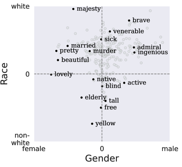
Figure 1: PMI analysis of our historical corpora. Words are placed on the intersectional gender/race plane.

The availability of large-scale digitised archives and modern NLP tools has enabled a number of sociological studies of historical trends and cultures (garg2018stereotypes; Kozlowski_2019; michel2011quantitative). Analyses of historical biases and stereotypes, in particular, can shed light on past societal dynamics and circumstances (sullam2022representation) and link them to contemporary challenges and biases prevalent in modern societies (payne2019slavery). For instance, payne2019slavery consider implicit bias as the cognitive residue of past and present structural inequalities and highlight the critical role of history in shaping modern forms of prejudice.

Thus far, previous research on bias in historical documents focused either on gender (rios-etal-2020-quantifying; wevers-2019-using) or ethnic biases (sullam2022representation). While garg2018stereotypes separately analyse both, their work does not engage with their intersection. Yet, in the words of crenshaw_mapping_1995, intersectional perspective is important because “the intersection of racism and sexism factors into black women’s lives in ways that cannot be captured wholly by looking separately at the race or gender dimensions of those experiences.”

Analysing historical documents poses particular challenges for modern NLP tools (nadav2023; ehrmann-etal-2020-language). Misspelt words due to wrongly recognised characters in the digitisation process, and archaic language unknown to modern NLP models, i.e. historical variant spellings and words that became obsolete in the current language, increase the task’s complexity (bollmann-2019-large; linharespontes:hal-02557116; piotrowski2012natural). However, while most previous work on historical NLP acknowledges the unique nature of the task, only a few address them within their experimental setup.

In this paper, we address the shortcomings of previous work and make the following contributions: (1) To the best of our knowledge, this paper presents the first study of historical language associated with entities at the intersections of two axes of oppression: race and gender. We study biases associated with identified entities on a word level, and to this end, employ distributional models and analyse semantics extracted from word embeddings trained on our historical corpora. (2) We conduct a temporal case study on historical newspapers from the Caribbean in the colonial period between 1770–1870. During this time, the region suffered both the consequences of European wars and political turmoil, as well as several uprisings of the local enslaved populations, which had a significant impact on the Caribbean social relationships and cultures (migge:halshs-00674699). (3) To address the challenges of analysing historical documents, we probe the applied methods for their stability and ability to comprehend the noisy, archaic corpora.

We find that there is a trade-off between the stability of word embeddings and their compatibility with the historical dataset. Further, our temporal analysis connects changes in biased word associations to historical shifts taking place in the period. For instance, we couple the high association between Caribbean countries and “manual labour” prevalent mostly in the earlier time periods to waves of white labour migrants coming to the Caribbean from 1750 onward. Finally, we provide evidence supporting the intersectionality theory by observing conventional manifestations of gender bias solely for white people. While unsurprising, this finding necessitates intersectional bias analysis for historical documents.

5.2 Related Work

Intersectional Biases.

Most prior work has analysed bias along one axis, e.g. race or gender, but not both simultaneously (field-etal-2021-survey; stanczak-etal-2021-survey). There, research on racial biases is generally centred around the gender majority group, such as Black men, while research on gender bias emphasises the experience of individuals who hold racial privilege, such as white women. Therefore, discrimination towards people with multiple minority identities, such as Black women, remains understudied. Addressing this, the intersectionality framework (Crenshaw1989-CREDTI) investigates how different forms of inequality, e.g. gender and race, intersect with and reinforce each other. Drawing on this framework, tan2019assessing; may-etal-2019-measuring; lepori-2020-unequal; maronikolakis-etal-2022-analyzing; guo2021detecting analyse the compounding effects of race and gender encoded in contextualised word representations and downstream tasks. Recently, lalor-etal-2022-benchmarking; jiang-fellbaum-2020-interdependencies show the harmful implications of intersectionality effects in pre-trained language models. Less interest has been dedicated to unveiling intersectional biases prevalent in natural language, with a notable exception of kim2020intersectional which provide evidence on intersectional bias in datasets of hate speech and abusive language on social media. As far as we know, this is the first paper on intersectional biases in historical documents.

Bias in Historical Documents.

Historical corpora have been employed to study societal phenomena such as language change (kutuzov-etal-2018-diachronic; hamilton-etal-2016-diachronic) and societal biases. Gender bias has been analysed in biomedical research over a span of 60 years (rios-etal-2020-quantifying), in English-language books published between 1520 and 2008 hoyle-etal-2019-unsupervised, and in Dutch newspapers from the second half of the 20th century (wevers-2019-using). sullam2022representation investigate the evolution of the discourse on Jews in France during the 19th century. garg2018stereotypes study the temporal change in stereotypes and attitudes toward women and ethnic minorities in the 20th and 21st centuries in the US. However, they neglect the emergent intersectionality bias.

When analysing the transformations of biases in historical texts, researchers rely on conventional tools developed for modern language. However, historical texts can be viewed as a separate domain due to their unique challenges of small and idiosyncratic corpora and noisy, archaic text (piotrowski2012natural). Prior work has attempted to overcome the challenges such documents pose for modern tools, including recognition of spelling variations (bollmann-2019-large) and misspelt words (boros-etal-2020-alleviating), and ensuring the stability of the applied methods (antoniak-mimno-2018-evaluating).

We study the dynamics of intersectional biases and their manifestations in language while addressing the challenges of historical data.

5.3 Datasets

Source	$\#$Files	$\#$Sentences
Caribbean Project	$7\,487$	$5\,224\,591$
Danish Royal Library	$5\,661$	$657\,618$
Total	$13\,148$	$5\,882\,209$

Table 1: Statistics of the newspapers dataset.

Period	Decade	$\#$Issues	Total
International	1710–1770	15	$1\,886$
conflicts	1770s	747
and slave	1780s	283
rebellions	1790s	841
Revolutions	1800s	604	$3\,790$
and nation	1810s	$1\,347$
building	1820s	$1\,839$
	1830s	$1\,838$	$7\,453$
Abolishment	1840s	$1\,197$
of slavery	1850s	$1\,111$
	1860s	$1\,521$
	1870s	$1\,786$

Table 2: Total number of articles in each period and decade.

Newspapers are considered an excellent source for the study of societal phenomena since they function as transceivers – both producing and demonstrating public discourse (wevers-2019-using). As part of this study, we collect newspapers written in English from the “Caribbean Newspapers, 1718–1876” database, the largest collection of Caribbean newspapers from the 18th–19th century available online. We extend this dataset with English-Danish newspapers published between 1770–1850 in the Danish colony of Santa Cruz (Saint Croix) downloaded from Danish Royal Library’s website. See Tab 1 and Fig 8 (in Section 5.8.1.1) for details.

As mentioned in §5.1, the Caribbean islands experienced significant changes and turmoils during the 18th–19th century. Although chronologies can change from island to island, key moments in Caribbean history can be divided into roughly four periods (higman_2021; heuman2013caribbean): 1) colonial trade and plantation system (1718 to 1750); 2) international conflicts and slave rebellions (1751 to 1790); 3) revolutions and nation building (1791 to 1825); 4) end of slavery and decline of European dominance (1826 to 1876). In our experimental setup, we conduct a temporal study on data split into these periods (see Tab 2 for the number of articles in each period). As the resulting number of newspapers for the first period is very small ($<$ 10), we focus on the three latter periods.

Figure 2: An example of a scanned newspaper (a) and the output of the OCR tool Tesseract (b). We fix simple OCR errors (highlighted) using a rule-based approach.

Data Preprocessing.

Starting with the scans of entire newspaper issues (Fig 2.a), we first OCR them using the popular software Tesseract with default parameters and settings. We then clean the dataset by applying the DataMunging package, which uses a simple rule-based approach to fix basic OCR errors (e.g. long s’ being OCRed as f’, (Fig 2.b)). As some of the newspapers downloaded from the Danish royal library contain Danish text, we use spaCy to tokenise the OCRed newspapers into sentences and the python package langdetect to filter out non-English sentences.

5.4 Bias and its Measures

Biases can manifest themselves in natural language in many ways (see the surveys by stanczak-etal-2021-survey; field-etal-2021-survey; lalor-etal-2022-benchmarking). In the following, we state the definition of bias we follow and describe the measures we use to quantify it.

5.4.1 Definition

Language is known to reflect common perceptions of the world (hitti-etal-2019-proposed) and differences in its usage have been shown to reflect societal biases (hoyle-etal-2019-unsupervised; marjanovic2022quantifying). In this paper, we define bias in a text as the use of words or syntactic constructs that connote or imply an inclination or prejudice against a certain sensitive group, following the bias definition as in hitti-etal-2019-proposed. To quantify bias under this definition, we analyse word embeddings trained on our historical corpora. These representations are assumed to carry lexical semantic meaning signals from the data and encode information about language usage in the proximity of entities. However, even words that are not used as direct descriptors of an entity influence its embedding, and thus its learnt meaning. Therefore, we further conduct an analysis focusing exclusively on words that describe identified entities.

5.4.2 Measures

WEAT The Word Embedding Association Test (Caliskan_2017) is arguably the most popular benchmark to assess bias in word embeddings and has been adapted in numerous research (may-etal-2019-measuring; rios-etal-2020-quantifying). WEAT employs cosine similarity to measure the association between two sets of attribute words and two sets of target concepts. Here, the attribute words relate to a sensitive attribute (e.g. male and female), whereas the target concepts are composed of words in a category of a specific domain of bias (e.g. career- and family-related words). For instance, the WEAT statistic informs us whether the learned embeddings representing the concept of $family$ are more associated with females compared to males. According to Caliskan_2017, the differential association between two sets of target concept embeddings, denoted $X$ and $Y$, with two sets of attribute embeddings, denoted as $A$ and $B$, can be calculated as:

$$s(X,Y,A,B)=\sum_{x\in X}\text{s}(x,A,B)-\sum_{y\in Y}\text{s}(y,A,B)$$

where $s(w,A,B)$ measures the embedding association between one target word $w$ and each of the sensitive attributes:

$$s(w,A,B)=\underset{a\in A}{\text{mean}}[\text{cos}(w,a)]-\underset{b\in B}{\text{mean}}[\text{cos}(w,b)]$$

The resulting effect size is then a normalised measure of association:

$$d=\frac{\underset{x\in X}{\text{mean}}[\text{s}(x,A,B)]-\underset{y\in Y}{\text{mean}}[\text{s}(y,A,B)]}{\underset{w\in X\cup Y}{\text{std}}[\text{s}(w,A,B)]}$$

As a result, larger effect sizes imply a more biased word embedding. Furthermore, concept-related words should be equally associated with either sensitive attribute group assuming an unbiased word embedding.

PMI We use point-wise mutual information (PMI; church-hanks-1990-word) as a measure of association between a descriptive word and a sensitive attribute (gender or race). In particular, PMI measures the difference between the probability of the co-occurrence of a word and an attribute, and their joint probability if they were independent as:

$$\text{PMI}(a,w)=\log\frac{p(a,w)}{p(a)p(w)}$$ (5.1)

A strong association with a specific gender or race leads to a high PMI. For example, a high value for $\text{PMI}(female,wife)$ is expected due to their co-occurrence probability being higher than the independent probabilities of $\mathit{female}$ and $\mathit{wife}$. Accordingly, in an ideal unbiased world, words such as $\mathit{honourable}$ would have a PMI of approximately zero for all gender and racial identities.

5.5 Experimental Setup

We perform two sets of experiments on our historical newspaper corpus. First, before we employ word embeddings to measure bias, we investigate the stability of the word embeddings trained on our dataset and evaluate their understanding of the noisy nature of the corpora. Second, we assess gender and racial biases using tools defined in §5.4.2.

5.5.1 Embedding Stability Evaluation

We use word embeddings as a tool to quantify historical trends and word associations in our data. However, prior work has called attention to the lack of stability of word embeddings trained on small and potentially idiosyncratic corpora (antoniak-mimno-2018-evaluating; gonen-etal-2020-simple). We compare these different embeddings setups by testing them with regard to their stability and capturing meaning while controlling for the tokenisation algorithm, embedding size and the minimum number of occurrences.

We construct word embeddings employing the continuous skip-gram negative sampling model from Word2vec (mikolov2013word) using gensim. Following prior work (antoniak-mimno-2018-evaluating; gonen-etal-2020-simple), we test two common vector dimension sizes of 100 and 300, and two minimum numbers of occurrences of 20 and 100. The rest of the hyperparameters are set to their default value. We use two different methods for tokenising documents, the spaCy tokeniser and a subword-based tokeniser, Byte-Pair Encoding (BPE, gage1994bpe). We train the BPE tokeniser on our dataset using the Hugging Face tokeniser implementation.

For each word in the vocabulary, we identify its 20 nearest neighbours and calculate the Jaccard similarity across five algorithm runs. Next, we test how well the word embeddings deal with the noisy nature of our documents. We create a list of 110 frequently misspelt words (See Section 5.8.1.2). We construct the list by first tokenising our dataset using spaCy and filtering out proper nouns and tokens that appear in the English dictionary. We then order the remaining tokens by frequency and manually scan the top $1\,000$ tokens for misspelt words. We calculate the percentage of words (averaged across 5 runs) for which the misspelt word is in immediate proximity to the correct word (top 5 nearest neighbours in terms of cosine similarity).

Based on the results of the stability and compatibility study, we select the most suitable model with which we conduct the following bias evaluation.

5.5.2 Bias Estimation

5.5.2.1 WEAT Evaluation

As discussed in §5.4.2, WEAT is used to evaluate how two attributes are associated with two target concepts in an embedding space, here of the model that was selected by the method described in §5.5.1.

In this work, we focus on the attribute pairs (female, male) and (white, non-white). Usually, comparing the sensitive attributes (white, non-white) is done by collecting the embedding of popular white names and popular non-white names tan2019assessing. However, this approach can introduce noise when applied to our dataset (handler1996slave). First, non-whites are less likely to be mentioned by name in historical newspapers compared to whites. Second, popular non-white names of the 18th and 19th centuries differ substantially from popular non-white names of modern times, and, to the best of our knowledge, there is no list of common historical non-white names. For these reasons, instead of comparing the pair (white, non-white), we compare the pairs (African countries, European countries) and (Caribbean countries, European countries).

Following rios-etal-2020-quantifying, we analyse the association of the above-mentioned attributes to the target concepts (career, family), (strong, weak), (intelligence, appearance), and (physical illness, mental illness). Following a consultation with a historian, we add further target concepts relevant to this period (manual labour, non-manual labour) and (crime, lawfulness). Tab 6 (in Section 5.8.1.3) lists the target and attribute words we use for our analysis.

We also train a separate word embedding model on each of the dataset splits defined in §5.3 and run WEAT on the resulting three models. Comparing the obtained WEAT scores allows us to visualise temporal changes in the bias associated with the attributes and understand its dynamics.

5.5.2.2 PMI Evaluation

Different from WEAT, calculating PMI requires first identifying entities in the OCRed historical newspapers and then classifying them into pre-defined attribute groups. The next step is collecting descriptors, i.e. words that are used to describe the entities. Finally, we use PMI to measure the association strength of the collected descriptors with each attribute group.

Entity Extraction.

We apply F-coref otmazgin-etal-2022-f, a model for English coreference resolution that simultaneously performs entity extraction and coreference resolution on the extracted entities. The model’s output is a set of entities, each represented as a list of all the references to that entity in the text. We filter out non-human entities by using nltk’s WordNet package, retaining only entities for which the synset “person.n1” is a hypernym of one of their references.

$\#$Entities	$\#$Males	$\#$Females	$\#$Non-whites	$\#$Non-white
				males	females
$601\,468$	$387\,292$	$78\,821$	$8\,525$	$4\,543$	$1\,548$

Table 3: The entities in our Caribbean newspapers dataset. Notice that $\#$males and $\#$females do not sum to $\#$entities as some entities could not be classified. Similarly, $\#$non-white males and $\#$non-white females do not sum to $\#$non-whites.

Entity Classification.

We use a keyword-based approach (lepori-2020-unequal) to classify the entities into groups corresponding to the gender and race axes and their intersection. Specifically, we classify each entity as being a member of male vs female, and white vs non-white. Additionally, entities are classified into intersectional groups (e.g. we classify an entity into the group non-white females if it belongs to both female and non-white).

Formally, we classify an entity $e$ with references $\{r^{1}_{e},...,r^{m}_{e}\}$ to attribute group $G$ with keyword-set $K_{G}=\{k_{1},...,k_{n}\}$ if $\exists i$ such that $r_{e}^{i}\in K_{G}$. See Section 5.8.1.3 for listing the keyword sets of the different groups. In Tab 3, we present the number of entities classified into each group. We note here the unbalanced representation of the groups in the dataset. Further, it is important to state, that because it is highly unlikely that an entity in our dataset would be explicitly described as white, we classify an entity into the whites group if it was not classified as non-white. See the Limitations section for a discussion of the limitations of using a keyword-based classification approach.

To evaluate our classification scheme, an author of this paper manually labelled a random sample of 56 entities. The keyword-based approach assigned the correct gender and race label for $\sim 80\%$ of the entities. See additional details in Tab 7 in Section 5.8.2. From a preliminary inspection, it appears that many of the entities that were wrongly classified as female were actually ships or other vessels (traditionally “ship” has been referred to using female gender). As F-coref was developed and trained using modern corpora, we evaluate its accuracy on the same set of 56 entities. Two authors of this paper validated its performance on the historical data to be satisfactory, with especially impressive results on shorter texts with fewer amount of OCR errors.

Descriptors Collection.

Finally, we use spaCy to collect descriptors for each classified entity. Here, we define the descriptors as the lemmatised form of tokens that share a dependency arc labelled “amod” (i.e. adjectives that describe the tokens) to one of the entity’s references. Every target group $G_{j}$ is then assigned with descriptors list $D_{j}=[d_{1},...,d_{k}]$.

To calculate PMI according to Eq 5.1, we estimate the joint distribution of a target group and a descriptor using a simple plug-in estimator:

$$\widehat{p}(G_{j},d_{i})\propto\mathrm{count}(G_{j},d_{i})$$ (5.2)

Now, we can assign every word $d_{i}$ two continuous values representing its bias in the gender and race dimensions by calculating $\text{PMI}(\textit{female},d_{i})-\text{PMI}(\textit{males},d_{i})$ and $\text{PMI}(\textit{non-white},d_{i})-\text{PMI}(\textit{white},d_{i})$. These two continuous values can be seen as $d_{i}$’s coordinates on the intersectional gender/race plane.

Tokenisation	Embedding Size	Min Freq	Mean JS Top 20	Correct Word in Top 5 (all words)	% Misspelling in vocabulary
BPE	100	20	0.66	37.04	94.44
	100	100	0.66	37.04	94.44
	300	20	0.63	40.74	94.44
	300	100	0.64	39.81	94.44
SpaCy	100	20	0.59	63.89	74.07
	100	100	0.65	48.15	56.48
	300	20	0.55	63.89	74.07
	300	100	0.61	50.00	56.48

Table 4: Results of the stability analysis of different word embedding methods (measured with Jaccard similarity) and their compatibility with the historical corpora (ability to recognise misspelt words).

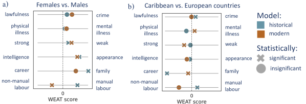
Figure 3: a) WEAT results of females vs males. The location of a marker measures the association strength of females with the concept (compared to males). For example, according to the modern model, females are associated with “weak” and non-manual labour while males are associated with “strong” and manual labour. b) WEAT results of Caribbean countries vs European countries. The location of a marker measures the association strength of Caribbean countries with the concept (compared to European countries).

Figure 4: Temporal WEAT analysis conducted for the periods 1751–1790 (rebellions), 1791–1825 (revolutions) and 1826–1876 (abolishment). Similar to Fig 3, the height of each bar represents how strong the association of the attribute is with each concept.

5.5.2.3 Lexicon Evaluation

Another popular approach for quantifying different aspects of bias is the application of specialised lexica (stanczak-etal-2021-survey). These lexica assign words a continuous value that represents how well the word aligns with a specific dimension of bias. We use NRC-VAD lexicon (mohammad-2018-obtaining) to compare word usage associated with the sensitive attributes race and gender in three dimensions: dominance (strength/weakness), valence (goodness/badness), and arousal (activeness/passiveness of an identity). Specifically, given a bias dimension $\mathcal{B}$ with lexicon ${L_{\mathcal{B}}}=\{(w_{1},a_{1}),...,(w_{n},a_{n})\}$, where $(w_{i},a_{i})$ are word-value pairs, we calculate the association of $\mathcal{B}$ with a sensitive attribute $G_{j}$ using:

$$\begin{split}A(\mathcal{B},G_{j})=\frac{\sum_{i}^{n}a_{i}\cdot\text{count}(w_{i},D_{j})}{\sum_{i}^{n}\text{count}(w_{i},D_{j})}\end{split}$$ (5.3)

where $\text{count}(w_{i},D_{j})$ is the number of times the word $w_{i}$ appears in the descriptors list $D_{j}$.

5.6 Results

First, we investigate which training strategies of word embeddings optimise their stability and compatibility on historical corpora (§5.6.1). Next, we analyse how bias is manifested along the gender and racial axes and whether there are any noticeable differences in bias across different periods of the Caribbean history (§5.6.2).

5.6.1 Embedding Stability Evaluation

In Tab 4, we present the results of the study on the influence of training strategies of word embeddings. We find that there is a trade-off between the stability of word embeddings and their compatibility with the dataset. While BPE achieves a higher Jaccard similarity across the top 20 nearest neighbours for each word across all runs, it loses the meaning of misspelt words. Interestingly, this phenomenon arises, despite the misspelt words occurring frequently enough to be included in the BPE model’s vocabulary.

For the remainder of the experiments, we aim to select a model which effectively manages this trade-off achieving both high stability and captures meaning despite the noisy nature of the underlying data. Thus, we opt to use a spaCy-based embedding with a minimum number of occurrences of 20 and an embedding size of 100 which achieves competitive results in both of these aspects. Finally, we note that our results remain stable across different algorithm runs and do not suffer from substantial variations which corroborates the reliability of the findings we make henceforth.

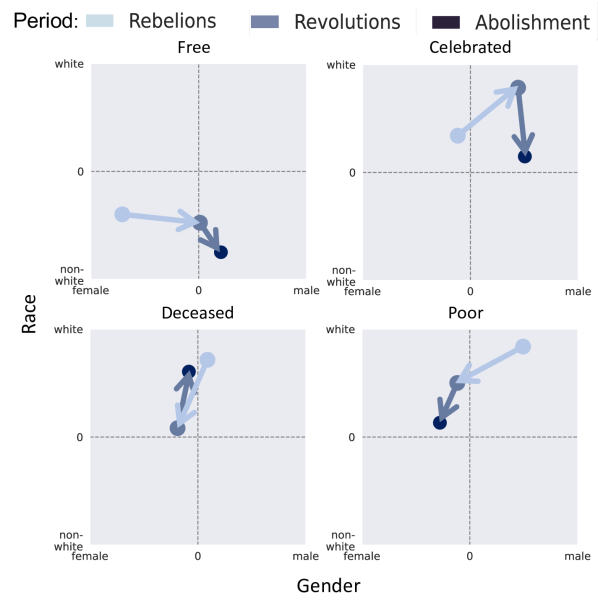
Figure 5: Intersectional PMI analysis of “free”, “celebrated”, “deceased” and “poor” across the periods.

5.6.2 Bias Estimation

5.6.2.1 WEAT Analysis

Fig 3 displays the results of performing a WEAT analysis for measuring the association of the six targets described in §5.5.2 with the attributes (females, males) and (Caribbean countries, European countries), respectively. We calculate the WEAT score using the embedding model from §5.6.1 and compare it with an embedding model trained on modern news corpora (word2vec-google-news-300, mikolov2013efficient). We notice interesting differences between the historical and modern embeddings. For example, while in our dataset females are associated with the target concept of manual labour, this notion is more aligned with males in the modern corpora. A likely cause is that during this period, womens’ intellectual and administrative work was not commonly recognised wayne2020women. It is also interesting to note that the attribute Caribbean countries has a much stronger association in the historical embedding with the target career (as opposed to family) compared to the modern embeddings. A possible explanation is that Caribbean newspapers referred to locals by profession or similar titles, while Europeans were referred to as relatives of the Caribbean population.

In Fig 4 and Fig 10 (in Section 5.8.2), we present a dynamic WEAT analysis that unveils trends on a temporal axis. In particular, we see an increase in the magnitude of association between the target of family vs career and the attributes (females, males) and (Caribbean countries, European countries) over time. It is especially interesting to compare Fig 3 with Fig 4. One intriguing result is that the high association between Caribbean countries and manual labour can be attributed to the earlier periods. This finding is potentially related to several historical shifts taking place in the period. For instance, while in the earlier years, it was normal for plantation owners to be absentees and continue to live in Europe, from 1750 onward, waves of white migrants with varied professional backgrounds came to the Caribbean.

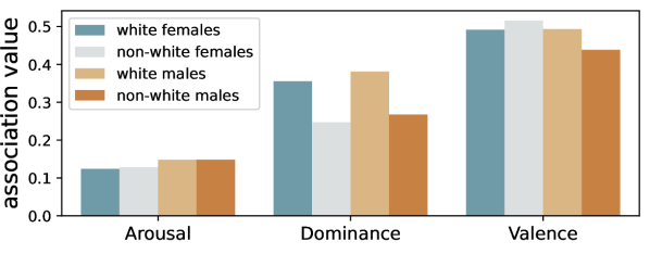
Figure 6: Association of attributes with the lexicon of dominance, valence, and arousal.

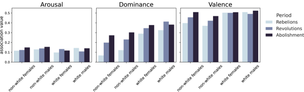
Figure 7: Association of attributes with the lexicon of dominance, valence, and value done on the periods 1751–1790 (rebellions), 1791–1825 (revolutions) and 1826–1876 (abolishment).

5.6.2.2 PMI Analysis

We report the results of the intersectional PMI analysis in Fig 1. As can be seen, an intersectional analysis can shed a unique light on the biased nature of some words in a way that single-dimensional analysis cannot. White males are “brave” and “ingenious”, and non-white males are described as “active” and “tall”. Interestingly, while words such as “pretty” and “beautiful” (and peculiarly, “murdered”) are biased towards white as opposed to non-white females, the word “lovely” is not, whereas “elderly” is strongly aligned with non-white females. Another intriguing dichotomy is the word pair “sick” and “blind” which are both independent along the gender axis but manifest a polar racial bias. In Tab 8 in Section 5.8.2, we list some examples from our dataset featuring those words.

Similarly to §5.6.2.1, we perform a temporal PMI analysis by comparing results obtained from separately analysing the three dataset splits. In Fig 5, we follow the trajectory over time of the biased words “free”, “celebrated”, “deceased” and “poor”. Each word displays different temporal dynamics. For example, while the word “free” moved towards the male attribute, “poor” transitioned to become more associated with the attributes female and non-white over time (potentially due to its meaning change from an association with poverty to a pity).

These results provide evidence for the claims of the intersectionality theory. We observe conventional manifestations of gender bias, i.e. “beautiful” and “pretty” for white females, and “ingenious” and “brave” for white males. While unsurprising due to the societal status of non-white people in that period, this finding necessitates intersectional bias analysis for historical documents in particular.

5.6.2.3 Lexicon Evaluation

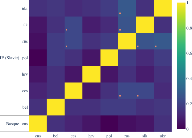
Figure 6: The percentage overlap between the top-50 most informative dimensions in a randomly selected language model for each of the morphosyntactic categories. Statistically significant overlap is marked with an orange square.

Figure 7: Animacy–m-BERT

Finally, we report the lexicon-based evaluation results in Fig 6 and Fig 7. Unsurprisingly, we observe lower dominance levels for the non-white and female attributes compared to white and male, a finding previously uncovered in modern texts (field-tsvetkov-2019-entity; rabinovich-etal-2020-pick). While Fig 7 indicates that the level of dominance associated with these attributes raised over time, a noticeable disparity to white males remains. Perhaps more surprising is the valence dimension. We see the highest and lowest levels of associations with the intersectional attributes non-white female and non-white male, respectively. We hypothesise that this connects to the nature of advertisements for lending the services of or selling non-white women where being agreeable is a valuable asset.

5.7 Conclusions

In this paper, we examine biases present in historical newspapers published in the Caribbean during the colonial era by conducting a temporal analysis of biases along the axes of gender, race, and their intersection. We evaluate the effectiveness of different embedding strategies and find a trade-off between the stability and compatibility of word representations on historical data. We link changes in biased word usage to historical shifts, coupling the development of the association between manual labour and Caribbean countries to waves of white labour migrants coming to the Caribbean from 1750 onward. Finally, we provide evidence to corroborate the intersectionality theory by observing conventional manifestations of gender bias solely for white people.

Limitations

We see several limitations regarding our work. First, we focus on documents in the English language only, neglecting many Caribbean newspapers and islands with other official languages. While some of our methods can be easily extended to non-English material (e.g. WEAT analysis), methods that rely on the pre-trained English model F-coref (i.e. PMI, lexicon-based analysis) can not.

On the same note, F-coref and spaCy were developed and trained using modern corpora, and their capabilities when applied to the noisy historical newspapers dataset, are noticeably lower compared to modern texts. Contributing to this issue is the unique, sometimes archaic language in which the newspapers were written. While we validate F-coref performance on a random sample (§5.5.2), this is a significant limitation of our work. Similarly, increased attention is required to adapt the keyword sets used by our methods to historical settings.

Moreover, our historical newspaper dataset is inherently imbalanced and skewed. As can be seen in Tab 2 and Fig 8, there is an over-representation of a handful of specific islands and time periods. While it is likely that in different regions and periods, less source material survived to modern times, part of the imbalance (e.g. the prevalence of the US Virgin Islands) can also be attributed to current research funding and policies. Compounding this further, minority groups are traditionally under-represented in news sources. This introduces noise and imbalance into our results, which rely on a large amount of textual material referring to each attribute on the gender/race plane that we analyse.

Relating to that, our keyword-based method of classifying entities into groups corresponding to the gender and race axes is limited. While we devise a specialised keyword set targeting the attributes female, male and non-white, we classify an entity into the white group if it was not classified as non-white. This discrepancy is likely to introduce noise into our evaluation, as can also be observed in Tab 7. This tendency may be intensified by the NLP systems that we use, as many tend to perform worse on gender- and race-minority groups (field-etal-2021-survey).

Finally, in this work, we explore intersectional bias only along the race and gender axes. Thus, we neglect the effects of other confounding factors (e.g. societal position, occupation) that affect asymmetries in language.

Ethical Considerations

Studying historical texts from the era of colonisation and slavery poses ethical issues to historians and computer scientists alike since vulnerable groups still suffer the consequences of this history in the present. Indeed, racist and sexist language is not only a historical artefact of bygone days but has a real impact on people’s lives (alim_oxford_2020).

We note that the newspapers we consider for this analysis were written foremost by the European oppressors. Moreover, only a limited number of affluent people (white males) could afford to place advertisements in those newspapers (which constitute a large portion of the raw material). This skews our study toward language used by privileged individuals and their perceptions.

This work aims to investigate racial and gender biases, as well as their intersection. Both race and gender are considered social constructs and can encompass a range of perspectives, including one’s reflected, observed, or self-perceived identity. In this paper, we classify entities as observed by the author of an article and infer their gender and race based on the pronouns and descriptors used in relation to this entity. We follow this approach in an absence of explicit demographic information. However, we warn that this method poses a risk of misclassification. Although the people referred to in the newspapers are no longer among the living, we should be considerate when conducting studies addressing vulnerable groups.

Finally, we use the mutually exclusive white and non-white race categories as well as male and female gender categories. We acknowledge that these groupings do not fully capture the nuanced nature of bias. This decision was made due to limited data discussing minorities in our corpus. While gender identities beyond the binary are unlikely to be found in the historical newspapers from the 18th-19th century, future work will aim to explore a wider range of racial identities.

Acknowledgements

This work is funded by Independent Research Fund Denmark under grant agreement number 9130-00092B, as well as the Danish National Research Foundation (DNRF 138). Isabelle Augenstein is further supported by the Pioneer Centre for AI, DNRF grant number P1.

5.8 Appendix

5.8.1 Additional Material

5.8.1.1 Dataset Statistics

In Fig 8, we present the geographical distribution of the newspapers in the curated dataset.

Figure 8: The geographical distribution of the curated Caribbean newspapers dataset.

5.8.1.2 Misspelt Words

Here we list 110 frequently misspelt words and their correct spelling, which was used for the embedding evaluation described in Section 5.5.1.

hon’ble - honorable, honble - honorable, majetty - majesty, mujesty - majesty, mojesty - majesty, houfe - house, calied - called, upen - upon, cailed - called, reeeived - received, betore - before, kaow - know, reecived - received, bope - hope, fonnd - found, dificult - difficult, qnite - quite, convineed - convinced, satistied - satisfied, intinate - intimate, demandcd - demanded, snecessful - successful, abie - able, impossibie - impossible, althouch - although, foreed - forced, giad - glad, preper - proper, understocd - understood, fuund - found, almest - almost, nore - more, atter - after, oceupied - occupied, understuod - understood, satis’y - satisfy, impofible - impossible, impoilible - impossible, inseusible - insensible, accessary - accesory, contident - confident, koown - known, receiv - receive, calied - calles, appellunt - appellant, Eniperor - emperor, auxious - anxious, ofien - often, lawiul - lawful, posstble - possible, Svanish - Spanish, fuffictent - sufficient, furcher - further, yery - very, uader - under, ayreeable - agreeable, ylad - glad, egreed - agreed, unabie - unable, giyen - given, uecessary - necessary, alrendy - already, entitied - entitled, cffered - offered, pesitive - positive, creater - creator, prefound - profound, examived - examined, successiul - successful, pablic - public, propor - proper, cousiderable - considerable, lcvely - lovely, fold - sold, seeond - second, huuse - house, excellen - excellent, auetion - auction, Engiand - England, peopie - people, goveroment - government, yeurs - years, exceliency - excellency, generel - general, foliowing - following, goneral - general, preperty - property, wondertul - wonderful, o’ciock - o’clock, exeellency - excellency, tollowing - following, Eugland - England, gentieman - gentleman, colontal - colonial, gevernment - government, excelleney - excellency, goverament - government, Lendon - London, Bermupa - Bermuda, goverument - government, himeelf - himself, entlemen - gentlemen, sublcriber - subscriber, majeliy - majesty, Weduesday - Wednesday, o’cleck - o’clock, o’cluck - o’clock, colonics - colonies, sngar - sugar.

5.8.1.3 Keyword Sets

Tab 5 and Tab 6 describe the various keyword sets that we used for entity classification (Section 5.5.2.2) and for performing the WEAT tests (Section 5.5.2.1.

Subgroup	Wordlist
Males	husband, suitor, brother, boyhood, beau, salesman, daddy, man, spokesman, chairman, lad, mister, men, sperm, dad, gelding, gentleman, boy, sir, horsemen, paternity, statesman, prince, sons, countryman, pa, suitors, stallion, fella, monks, fiance, chap, uncles, godfather, bulls, males, grandfather, penis, lions, nephew, monk, countrymen, grandsons, beards, schoolboy, councilmen, dads, fellow, colts, mr, king, father, fraternal,baritone, gentlemen, fathers, husbands, guy, semen, brotherhood, nephews, lion, lads, grandson, widower, bachelor, kings, male, son, brothers, uncle, brethren, boys, councilman, czar, beard, bull, salesmen, fraternity, dude, colt, john, he, himself, his
Females	sisters, queen, ladies, princess, witch, mother, nun, aunt, princes, housewife, women, convent, gals, witches, stepmother, wife, granddaughter, mis, widows, nieces, studs, niece, actresses, wives, sister, dowry, hens, daughters, womb, monastery, ms, misses, mama, mrs, fillies, woman, aunts, girl, actress, wench, brides, grandmother, stud, lady, female, maid, gal, queens, hostess, daughter, grandmothers, girls, heiress, moms, maids, mistress, mothers, mom, mare, filly, maternal, bride, widow, goddess, diva, maiden, hen, housewives, heroine, nuns, females’, she, herself, hers, her
Non-whites	negro, negros, creole, indian, negroes, colored, mulatto, mulattos, negresse, mundingo, brown, browns, african, congo, black, blacks, dark, creoles
Whites	(any entity that was not classified as Non-white)

Table 5: Keywords used for classification entities into subgroups.

Attribute	Wordlist
Males	husband, man, mister, gentleman, boy, sir, prince, countryman, fiance, godfather, grandfather, nephew, fellow, mr, king, father, guy, grandson, widower, bachelor, male, son, brother, uncle, brethren
Females	sister, queen, lady, witch, mother, aunt, princes, housewife, stepmother, wife, granddaughter, mis, niece, ms, misses, mrs, woman, girl, wench, bride, grandmother, female, maid, daughter, mistress, bride, widow, maiden
European countries	ireland, georgia, france, monaco, poland, cyprus, greece, hungary, norway, portugal, belgium, luxembourg, finland, albania, germany, netherlands, montenegro, scotland, spain, europe, russia, vatican, switzerland, lithuania, bulgaria, wales, ukraine, romania, denmark, england, italy, bosnia, turkey, malta, iceland, austria, croatia, sweden, macedonia
African countries	liberia, mozambique, gambia, ghana, morocco, chad, senegal, togo, algeria, egypt, benin, ethiopia, niger, madagascar, guinea, mauritius, africa, mali, congo, angola
Caribbean countries	barbuda, bahamas, jamaica, dominica, haiti, antigua, grenada, caribbean, barbados, cuba, trinidad, dominican, nevis, kitts, lucia, croix, tobago, grenadines, puerto, rico
Target	Wordlist
Appearance	apt, discerning, judicious, imaginative, inquiring, intelligent, inquisitive, wise, shrewd, logical, astute, intuitive, precocious, analytical, smart, ingenious, reflective, inventive, venerable, genius, brilliant, clever, thoughtful
Intelligence	bald, strong, muscular, thin, voluptuous, blushing, athletic, gorgeous, handsome, homely, feeble, fashionable, attractive, weak, plump, ugly, slim, stout, pretty, fat, sensual, beautiful, healthy, alluring, slender
Weak	failure, loser, weak, timid, withdraw, follow, fragile, afraid, weakness, shy, lose, surrender, vulnerable, yield
Strong	strong, potent, succeed, loud, assert, leader, winner, dominant, command, confident, power, triumph, shout, bold
Family	loved, sisters, mother, reunited, estranged, aunt, relatives, grandchildren, godmother, kin, grandsons, sons, son, parents, stepmother, childless, paramour, nieces, children, niece, father, twins, sister, fiance, daughters, youngest, uncle, uncles, aunts, eldest, cousins, grandmother, children, loving, daughter, paternal, girls, nephews, friends, mothers, grandfather, cousin, maternal, married, nephew, wedding, grandson
Career	branch, managers, usurping, subsidiary, engineering, performs, fiscal, personnel, duties, offices, clerical, engineer, executive, functions, revenues, entity, competitive, competitor, employing, chairman, director, commissions, audit, promotion, professional, assistant, company, auditors, oversight, departments, comptroller, president, manager, operations, marketing, directors, shareholder, engineers, corporate, salaries, internal, management, salaried, corporation, revenue, salary, usurpation, managing, delegated, operating

Target	Wordlist
Manual labour	sailor, bricklayer, server, butcher, gardener, cook, repairer, maid, guard, farmer, fisher, carpenter, paver, cleaner, cabinetmaker, barber, breeder, washer, miner, builder, baker, fisherman, plumber, labourer, servant
Non-manual labour	teacher, judge, manager, lawyer, director, mathematician, physician, medic, designer, bookkeeper, nurse, librarian, doctor, educator, auditor, clerk, midwife, translator, inspector, surgeon
Mental illness	sleep, pica, disorders, nightmare, personality, histrionic, stress, dependence, anxiety, terror, emotional, delusion, depression, panic, abuse, disorder, mania, hysteria
Physical illness	scurvy, sciatica, asthma, gangrene, gerd, cowpox, lice, rickets, malaria, epilepsy, sars, diphtheria, smallpox, bronchitis, thrush, leprosy, typhus, sids, watkins, measles, jaundice, shingles, cholera, boil, pneumonia, mumps, rheumatism, rabies, abscess, warts, plague, dysentery, syphilis, cancer, influenza, ulcers, tetanus
Crime	arrested, unreliable, detained, arrest, detain, murder, murdered, criminal, criminally, thug, theft, thief, mugger, mugging, suspicious, executed, illegal, unjust, jailed, jail, prison, arson, arsonist, kidnap, kidnapped, assaulted, assault, released, custody, police, sheriff, bailed, bail
lawfulness	loyal, charming, friendly, respectful, dutiful, grateful, amiable, honourable, honourably, good, faithfully, faithful, pleasant, praised, just, dignified, approving, approve, compliment, generous, faithful, intelligent, appreciative, delighted, appreciate

Table 6: Keywords used for performing WEAT evaluation.

5.8.2 Supplementary Results

In Tab 7, we report the accuracy of the classified entities using the keyword-based approach. In Tab 8, we list examples of sentences from our newspaper dataset. Fig 9 presents the WEAT results of the attributes African countries vs European countries. Fig 10 presents temporal WEAT analysis conducted for the attributes African countries vs European countries.

Attribute	Ratio of correctly classified entities	Ratio of incorrectly classified entities	Ratio of unable to classify
Non-whites	0.89	0.036	0.07
Whites	0.75	0.18	0.07
Males	0.89	0.036	0.07
Females	0.79	0.21	0

Table 7: Performance of the keyword-based classification approach.

Word	Sentence
ingenious	This comprehensive piece of clockwork cost the ingenious and indefatigable artist (one Jacob Lovelace, of Exeter,) 34 years’ labour.
elderly	y un away for upwards of 16 Months past;; elderly NEGRO WOMAN hamed LOUISA, belongifg to the Estate of the late Ancup.
active	FOR SALE, STRONG active NEGRO GIRL, about 24 Years of Age, she is a good Cook, can W asu, [rron, and is well acquainted with Housework in general.
beautiful	and the young husband was hurried away, being scarcely permitted to take a parting kiss from his blooming and beautiful bride.
blind	Dick, of the Mundingo Counrry, blind mark, about 18 years of ane, says he belongs te the estate Of ee Nichole, dec. of Mantego bay.
sick	The young wife had snatched upa,; few of her own and her baby’s clothes; the husband, | Openiug Chorus, though sick, had attended to his duty to the last, and es | Song caped penniless with the clothes on his back.
free	A free black girl JOSEPHINE, detained by the Police as being diseased; Proprietors and Managers an the Country are kindly requested to have the said Josephine apprehended ‘and lodged in the Towa Prison, the usual reward will be paid
brave	From that moment the brave Lopez Lara was only occupied in devising means for delivering this notorious criminal into the hvids of justice.

Table 8: Examples from our dataset that contain biased words. Notice the high levels of noise and OCR errors.

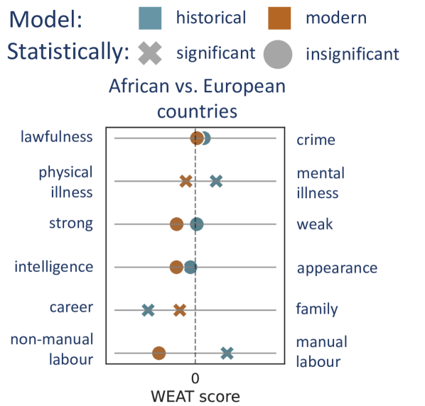
Figure 9: WEAT results of African countries vs European countries.

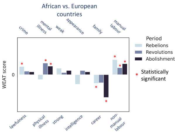
Figure 10: Temporal WEAT analysis conducted for the periods 1751–1790 (rebellions), 1791–1825 (revolutions) and 1826–1876 (abolishment). Similar to Fig 3, the height of each bar represents how strong the association of the attribute of African countries is with each concept.

Chapter 6 Grammatical Gender’s Influence on Distributional Semantics: A Causal Perspective

The work presented in this chapter was submitted to TACL and is currently under review.

Abstract

How much meaning influences gender assignment across languages is an active area of research in modern linguistics and cognitive science. We can view current approaches as aiming to determine where gender assignment falls on a spectrum, from being fully arbitrarily determined to being largely semantically determined. For the latter case, there is a formulation of the neo-Whorfian hypothesis, which claims that even inanimate noun gender influences how people conceive of and talk about objects (using the choice of adjective used to modify inanimate nouns as a proxy for meaning). We offer a novel, causal graphical model that jointly represents the interactions between a noun’s grammatical gender, its meaning, and adjective choice. In accordance with past results, we find a relationship between the gender of nouns and the adjectives which modify them. However, when we control for the meaning of the noun, we find that grammatical gender has a near-zero effect on adjective choice, thereby calling the neo-Whorfian hypothesis into question.

6.1 Introduction

Approximately half of the world’s languages have grammatical gender (wals-30), a grammatical phenomenon that groups nouns together into classes that share morphosyntactic properties (hockett-1958-course; corbett1991gender; kramer-2015-morphosyntax). Among languages that have gender, there is variation in the number of gender classes; for example, some languages have only two classes, e.g., all Danish nouns are classed as either common or neuter, whereas others have significantly more, e.g., Nigerian Fula has around 20, depending on the variety (Arnott-1967; Koval-1979; Breedveld-1995). Languages also vary with respect to how much gender assignment, i.e., how nouns are sorted into particular genders, is related to the form and the meaning of the noun (corbett1991gender; plaster-polinky-2007-women; wals-32; corbett-2014-gender; kramer-2020-grammatical; sahai-sharma-2021-predicting). Some languages group nouns into gender classes that are highly predictable from phonological (Parker-and-Hayward-1985; corbett1991gender; wals-32) or morphological (corbett1991gender; wals-32; corbett-fraser-2000-systems) information, while others, such as the Dagestanian languages Godoberi and Bagwalal, seem to be predictable from meaning (corbett1991gender; corbett-fraser-2000-systems; corbett-2014-gender)—although, even for most of the strictly semantic systems, there are exceptions.

Despite this variation, gender assignment is rarely, if ever, wholly predictable from meaning alone. In many languages, there is a semantic core of nouns that are conceptually coherent (aksenov-1984; corbett1991gender; williams-etal-2019-quantifying; kramer-2020-grammatical) and a surround that is somewhat less semantically coherent. Axes along which genders are conceptually coherent often include semantic properties of animate nouns, with inanimate nouns appearing in the surround. For example, in Spanish, despite the fact that the nouns table ( mesa in Spanish) and woman ( mujer in Spanish) appear in the same gender (i.e., feminine), it is hard to imagine what meaning they share. Indeed, some linguists posit that gender assignment for inanimate nouns is effectively arbitrary (bloomfield1935language; YAikhenvald2000-YAICAT-2; foundalis-2002-evolution). And, to the extent that gender assignment is not fully arbitrary for inanimate nouns (williams-etal-2021-relationships), many researchers argue there is no compelling evidence showing grammatical gender affects how we conceptualize objects (samuel-2019-grammatical) or the distributional properties of language (mickan2014key).

However, not all researchers agree that non-arbitrariness in gender assignment, to the extent it exists, should be assumed to have no bearing on language production. boroditsky2003linguistic famously argued for a causal relationship between the gender assigned to inanimate nouns and their usage, in a view colloquially known as the neo-Whorfian hypothesis after Benjamin Whorf (Whorf1956language). Proponents of this view have studied human associations, under the assumption that people’s perceptions of the genders of objects are strongly influenced by the grammatical genders these objects are assigned in their native language (boroditsky2003sex; Semenuks2017EffectsOG). One manifestation of this perception is the choice of adjectives used to describe nouns (Semenuks2017EffectsOG). While this is an intriguing possibility, there are additional lexical properties of nouns that may act as confounders and, thus, finding statistical evidence for the causal effect of grammatical gender on adjective choice requires great care.

To facilitate a cleaner way to reason about the causal influence grammatical gender may have on adjective usage, we introduce a causal graphical model to represent the interactions between an inanimate noun’s grammatical gender, its meaning, and the choice of its descriptors. This causal framework enables intervening on the values of specific factors to isolate the effects between various properties of languages. Our model explains the distribution of adjectives that modify a noun, conditioned on both a representation of the noun’s meaning and the gender of the noun itself. Upon estimation of the parameters of the causal graphical model, we test the neo-Whorfian hypothesis beyond the anecdotal level. First, we validate our model by comparing it to the method presented in prior work without any causal intervention. Second, we employ our model with a causal intervention on the noun meaning to test the neo-Whorfian hypothesis. That is, we ask a counterfactual question: Had nouns been lexicalized with different grammatical genders but retained their same meanings, would the distribution of adjectives that speakers use to modify them have been different? We quantify this difference in distributions information-theoretically, using the Jensen–Shannon divergence.

We employ our model on five languages that exhibit grammatical gender: four Indo-European languages (German, Polish, Portuguese, and Spanish) and one language from the Afro-Asiatic language family (Hebrew). We find that, at least in Wikipedia data, a noun’s grammatical gender is indeed correlated with the choice of its descriptors. However, when controlling for a confounder, nominal meaning, we present empirical evidence that noun gender has no significant effect on adjective usage. Our results provide evidence against the neo-Whorfian hypothesis.

6.2 A Primer on Grammatical Gender

In many languages with grammatical gender, adjectives, demonstratives, determiners, and other word categories agree with the noun in gender, i.e., they will systematically change in form to indicate the grammatical gender of the noun they modify. Observe the following sentence, A small dog sleeps under the tree., translated into two languages that exhibit grammatical gender (German and Polish):

1. Ein kleiner Hund schläft unter dem Baum. (de)
   a.M small.M dog.M is sleeping under the.M tree.M

2. Mały pies śpi pod drzewem. (pl)
   a.M small.M dog.M is sleeping under the.N tree.N

Because the German (de) and Polish (pl) words for a dog, Hund and pies, are both assigned masculine gender, the adjectives in the respective languages, klein and mały, are morphologically gender-marked as masculine. Additionally, in German, the article, dem, is also gender-marked as masculine. The fact that gender is reflected by agreement patterns on other elements is generally taken to be a definitional property (hockett-1958-course; corbett1991gender; kramer-2020-grammatical) separating gender from other kinds of noun classification systems, such as numeral classifiers or declension classes.

It is an undeniable fact in many languages that morphological agreement reflects the gender of a noun in the form of other elements. However, one could imagine a similar process, such as analogical reasoning (lucy-2016-recent), by which gender could influence an adjective’s meaning instead of just its form. If a noun’s meaning were to influence its gender, then the noun meaning could also indirectly influence adjective usage, by way of the relationship between grammatical gender and adjective usage. There is ample statistical evidence that grammatical gender assignment is not fully arbitrary (williams-etal-2019-quantifying; williams-etal-2021-relationships; nelson2005french; sahai-sharma-2021-predicting). Such evidence is prima facie consistent with the idea that such influence is conceivably possible.

However, it is important to note that claims that noun gender influences meaning are by their very nature causal claims. The most famous example of such a causal claim is the neo-Whorfian view of gender (boroditsky2003sex; boroditsky2001does; boroditsky2003linguistic), which states that a noun’s grammatical gender causally affects meaning (e.g., adjective choice). This view can be summed up in the following quote from boroditsky2003sex, “people’s ideas about the genders of objects are strongly influenced by the grammatical genders assigned to these objects in their native language” (emphasis ours). Despite this clear causal formulation of the hypothesis, there has yet to be a modeling approach developed to test it.

Laboratory studies have been used to gather evidence for the neo-Whorfian hypothesis. For example, Semenuks2017EffectsOG perform a small laboratory experiment involving human participants to explore whether noun gender affects a particular proxy for meaning, adjective choice. This work found that, in languages where bridge is feminine (like German; Brücke), participants modified it with adjectives that are stereotypically used to refer to women, such as beautiful, and in languages where bridge is masculine (like Spanish; puente), they used adjectives stereotypically used to refer to men, like sturdy. Subsequent studies, however, have failed to replicate this result, raising into question the strength of this relationship between gender and adjective usage (mickan2014key).

Our paper builds on williams-etal-2021-relationships correlational study of noun meaning and its distributional properties and advances it to a causal one. While williams-etal-2021-relationships report a non-trivial, statistically significant mutual information between the grammatical gender of a noun and its modifiers, e.g., adjectives that modify the noun, they do not control for other factors which might influence adjective usage, most notably the lexical semantics of the noun. Mutual information on its own cannot speak to causation. We are thus motivated by a potential common-cause effect whereby the lexical semantics jointly influences a noun’s grammatical gender and its distribution over modifiers and propose a causal model.

6.3 A Causal Graphical Model

The technical contribution of this work is a novel causal graphical model for jointly representing the relationship between the grammatical gender of a noun, its meaning, and descriptors. This model is depicted in Fig 1. If properly estimated, the model should enable us to measure the causal effect of grammatical gender on adjective choice in language. We first develop the necessary notation.

Notation

We follow several font and coloring conventions to make our notation easier to digest. All base sets will be uppercase and in calligraphic font, e.g., $\mathcal{X}$. Elements of $\mathcal{X}$ will be lowercase and italicized, e.g., $x\in\mathcal{X}$. Subsets (including submultisets) will be uppercase and unitalicized, e.g., $\mathrm{X}\subset\mathcal{X}$. Random variables that draw their values from $\mathcal{X}$ will be uppercase and italicized, e.g., $p(X=x)$. We will use three colors. Those objects that relate to nouns will be in blue, those objects that relate to adjectives will be in purple, and those objects that relate to gender will be in green.

6.3.1 The Model

We assume there exists a set of nominal meanings ${\color[rgb]{0.14453125,0.43359375,0.68359375}\boldsymbol{\mathcal{N}}}$. In this paper, we assume that such meanings are representable by vectors in $\mathbb{R}^{D}$. We denote the elements of ${\color[rgb]{0.14453125,0.43359375,0.68359375}\boldsymbol{\mathcal{N}}}$ as ${\color[rgb]{0.14453125,0.43359375,0.68359375}\boldsymbol{n}}\in\mathbb{R}^{D}$. Additionally, we assume there exists an alphabet of adjectives ${\color[rgb]{0.5859375,0.16796875,0.375}\mathcal{A}}$. We denote an element of ${\color[rgb]{0.5859375,0.16796875,0.375}\mathcal{A}}$ as ${\color[rgb]{0.5859375,0.16796875,0.375}a}$. Finally, we assume there exists a language-dependent set of ${\color[rgb]{0.45703125,0.6171875,0.546875}\mathcal{G}}$. In Spanish, for instance, we would have ${\color[rgb]{0.45703125,0.6171875,0.546875}\mathcal{G}}=\{{\color[rgb]{0.45703125,0.6171875,0.546875}\textsc{fem}},{\color[rgb]{0.45703125,0.6171875,0.546875}\textsc{msc}}\}$ whereas in German ${\color[rgb]{0.45703125,0.6171875,0.546875}\mathcal{G}}=\{{\color[rgb]{0.45703125,0.6171875,0.546875}\textsc{fem}},{\color[rgb]{0.45703125,0.6171875,0.546875}\textsc{msc}},{\color[rgb]{0.45703125,0.6171875,0.546875}\textsc{neu}}\}$. We denote elements of ${\color[rgb]{0.45703125,0.6171875,0.546875}\mathcal{G}}$ as ${\color[rgb]{0.45703125,0.6171875,0.546875}g}$.

We now develop a generative model of the subset of lexical semantics relating to adjective choice. We wish to generate a set of ${\color[rgb]{0.14453125,0.43359375,0.68359375}\boldsymbol{\mathcal{N}}}$ nouns, each of which is modified by a multiset of adjectives. We can view this model as a partial generative model of a corpus where we focus on generating noun types and adjective tokens. Generation from the model proceeds as follows:

$${\color[rgb]{0.14453125,0.43359375,0.68359375}\boldsymbol{n}}\sim p_{{\color[rgb]{0.14453125,0.43359375,0.68359375}{N}}}(\cdot)$$

$$\quad\quad{\color[rgb]{.5,.5,.5}(\text{sample a noun meaning }{\color[rgb]{0.14453125,0.43359375,0.68359375}\boldsymbol{n}})}$$

$${\color[rgb]{0.45703125,0.6171875,0.546875}g}_{{\color[rgb]{0.14453125,0.43359375,0.68359375}\boldsymbol{n}}}\sim p_{{\color[rgb]{0.45703125,0.6171875,0.546875}{G}}}(\cdot\mid{\color[rgb]{0.14453125,0.43359375,0.68359375}\boldsymbol{n}})$$

$$\quad\quad{\color[rgb]{.5,.5,.5}(\text{sample the gender }{\color[rgb]{0.45703125,0.6171875,0.546875}g}_{{\color[rgb]{0.14453125,0.43359375,0.68359375}\boldsymbol{n}}}\text{ assigned to }{\color[rgb]{0.14453125,0.43359375,0.68359375}\boldsymbol{n}})}$$

$${\color[rgb]{0.5859375,0.16796875,0.375}a}_{{\color[rgb]{0.14453125,0.43359375,0.68359375}\boldsymbol{n}}}\sim p_{{\color[rgb]{0.5859375,0.16796875,0.375}{A}}}(\cdot\mid{\color[rgb]{0.14453125,0.43359375,0.68359375}\boldsymbol{n}},{\color[rgb]{0.45703125,0.6171875,0.546875}g}_{{\color[rgb]{0.14453125,0.43359375,0.68359375}\boldsymbol{n}}})$$

$$\quad\quad{\color[rgb]{.5,.5,.5}(\text{sample adjectives }{\color[rgb]{0.5859375,0.16796875,0.375}a}_{{\color[rgb]{0.14453125,0.43359375,0.68359375}\boldsymbol{n}}}\text{ that modify }{\color[rgb]{0.14453125,0.43359375,0.68359375}\boldsymbol{n}})}$$

In this formulation, ${\color[rgb]{0.14453125,0.43359375,0.68359375}{N}}$ is a ${\color[rgb]{0.14453125,0.43359375,0.68359375}\boldsymbol{\mathcal{N}}}$-valued random variable, ${\color[rgb]{0.45703125,0.6171875,0.546875}{G}}$ is a ${\color[rgb]{0.45703125,0.6171875,0.546875}\mathcal{G}}$-valued random variable, and ${\color[rgb]{0.5859375,0.16796875,0.375}{A}}$ is a ${\color[rgb]{0.5859375,0.16796875,0.375}\mathcal{A}}$-valued random variable.

Written as a probability distribution, we have

$$p( \{{\color[rgb]{0.5859375,0.16796875,0.375}\mathrm{A}}_{{\color[rgb]{0.14453125,0.43359375,0.68359375}\boldsymbol{n}}}\},\{{\color[rgb]{0.45703125,0.6171875,0.546875}g}_{{\color[rgb]{0.14453125,0.43359375,0.68359375}\boldsymbol{n}}}\},{\color[rgb]{0.14453125,0.43359375,0.68359375}\mathrm{N}})$$ (6.1)

$$=\prod_{{\color[rgb]{0.14453125,0.43359375,0.68359375}\boldsymbol{n}}\in{\color[rgb]{0.14453125,0.43359375,0.68359375}\mathrm{N}}}\prod_{{\color[rgb]{0.5859375,0.16796875,0.375}a}\in{\color[rgb]{0.5859375,0.16796875,0.375}\mathrm{A}}_{{\color[rgb]{0.14453125,0.43359375,0.68359375}\boldsymbol{n}}}}\,p_{{\color[rgb]{0.5859375,0.16796875,0.375}{A}}}({\color[rgb]{0.5859375,0.16796875,0.375}a}\mid{\color[rgb]{0.14453125,0.43359375,0.68359375}\boldsymbol{n}},{\color[rgb]{0.45703125,0.6171875,0.546875}g}_{{\color[rgb]{0.14453125,0.43359375,0.68359375}\boldsymbol{n}}})\,p_{{\color[rgb]{0.45703125,0.6171875,0.546875}{G}}}({\color[rgb]{0.45703125,0.6171875,0.546875}g}_{{\color[rgb]{0.14453125,0.43359375,0.68359375}\boldsymbol{n}}}\mid{\color[rgb]{0.14453125,0.43359375,0.68359375}\boldsymbol{n}})\,p_{{\color[rgb]{0.14453125,0.43359375,0.68359375}{N}}}({\color[rgb]{0.14453125,0.43359375,0.68359375}\boldsymbol{n}})$$

where ${\color[rgb]{0.14453125,0.43359375,0.68359375}\mathrm{N}}\subset{\color[rgb]{0.14453125,0.43359375,0.68359375}\boldsymbol{\mathcal{N}}}$ is a subset of the set of nominal meanings and each ${\color[rgb]{0.45703125,0.6171875,0.546875}g}_{\color[rgb]{0.14453125,0.43359375,0.68359375}\boldsymbol{n}}\in{\color[rgb]{0.45703125,0.6171875,0.546875}\mathcal{G}}$ is the gender of ${\color[rgb]{0.14453125,0.43359375,0.68359375}\boldsymbol{n}}$, and each ${\color[rgb]{0.5859375,0.16796875,0.375}\mathrm{A}}_{{\color[rgb]{0.14453125,0.43359375,0.68359375}\boldsymbol{n}}}\subset{\color[rgb]{0.5859375,0.16796875,0.375}\mathcal{A}}$ is a multisubset of ${\color[rgb]{0.5859375,0.16796875,0.375}\mathcal{A}}$ that contains the observed adjectives that modify ${\color[rgb]{0.14453125,0.43359375,0.68359375}\boldsymbol{n}}$. This model is represented graphically in Fig 1, where the arrow from ${\color[rgb]{0.14453125,0.43359375,0.68359375}{N}}$ to ${\color[rgb]{0.45703125,0.6171875,0.546875}{G}}$ represents the dependence of ${\color[rgb]{0.45703125,0.6171875,0.546875}{G}}$ on ${\color[rgb]{0.14453125,0.43359375,0.68359375}{N}}$ as shown in the conditional probability distribution $p_{{\color[rgb]{0.45703125,0.6171875,0.546875}{G}}}({\color[rgb]{0.45703125,0.6171875,0.546875}g}_{{\color[rgb]{0.14453125,0.43359375,0.68359375}\boldsymbol{n}}}\mid{\color[rgb]{0.14453125,0.43359375,0.68359375}\boldsymbol{n}})$, and the arrows from ${\color[rgb]{0.14453125,0.43359375,0.68359375}\boldsymbol{n}}$ and ${\color[rgb]{0.45703125,0.6171875,0.546875}g}$ to ${\color[rgb]{0.5859375,0.16796875,0.375}a}$ represent the potential dependence of ${\color[rgb]{0.5859375,0.16796875,0.375}a}$ on ${\color[rgb]{0.14453125,0.43359375,0.68359375}\boldsymbol{n}}$ and ${\color[rgb]{0.45703125,0.6171875,0.546875}g}$, as shown in the conditional probability distribution $p_{{\color[rgb]{0.5859375,0.16796875,0.375}{A}}}({\color[rgb]{0.5859375,0.16796875,0.375}a}\mid{\color[rgb]{0.14453125,0.43359375,0.68359375}\boldsymbol{n}},{\color[rgb]{0.45703125,0.6171875,0.546875}g}_{{\color[rgb]{0.14453125,0.43359375,0.68359375}\boldsymbol{n}}})$.

Importantly, our model generates the lexical semantics of noun types. This means that a sample from it generates a new noun, whose semantics we may never have seen before. If we are able to estimate such a model well, we can use the basics of causal inference to estimate the causal effect gender has on adjective usage. Specifically, as is clear from Fig 1, the only confounder between gender and adjective selection in our proposed model is the semantics of the noun.

Figure 1: Causal graphical model relating noun semantics, gender, and adjective choice. The neo-Whorfian hypothesis posits that a noun’s gender causally influences adjective choice. Correctly evaluating this hypothesis must also account for the relationship between the noun’s meaning and adjective choice.

6.3.2 Intervention

Thus, to the extent that the modeler believes our model $p$ is a reasonable generative model of lexical semantics, we apply Pearl’s backdoor criterion to get a causal effect (pearl1993bayesian). One does so by applying the do-calculus, which results in the following gender-specific distribution over adjectives

$$p({\color[rgb]{0.5859375,0.16796875,0.375}a}\mid \,\mathrm{do}({\color[rgb]{0.45703125,0.6171875,0.546875}{G}}={\color[rgb]{0.45703125,0.6171875,0.546875}g}))$$ (6.2)

$$=\sum_{{\color[rgb]{0.14453125,0.43359375,0.68359375}\boldsymbol{n}}\in{\color[rgb]{0.14453125,0.43359375,0.68359375}\boldsymbol{\mathcal{N}}}}p_{{\color[rgb]{0.5859375,0.16796875,0.375}{A}}}\left({\color[rgb]{0.5859375,0.16796875,0.375}a}\mid{\color[rgb]{0.45703125,0.6171875,0.546875}{G}}={\color[rgb]{0.45703125,0.6171875,0.546875}g},{\color[rgb]{0.14453125,0.43359375,0.68359375}\boldsymbol{n}}\right)p_{{\color[rgb]{0.14453125,0.43359375,0.68359375}{N}}}({\color[rgb]{0.14453125,0.43359375,0.68359375}\boldsymbol{n}})$$

where for simplicity, ${\color[rgb]{0.14453125,0.43359375,0.68359375}\boldsymbol{\mathcal{N}}}$ is assumed to be at most countable despite being a subset of $\mathbb{R}^{D}$. We are now interested in using $p({\color[rgb]{0.5859375,0.16796875,0.375}a}\mid\mathrm{do}({\color[rgb]{0.45703125,0.6171875,0.546875}{G}}={\color[rgb]{0.45703125,0.6171875,0.546875}g}))$ to measure the extent to which a nominal meaning’s grammatical gender in a language influences which adjectives are used to describe that noun. In particular, we aim to measure how different the adjective choice would be if the noun had a different grammatical gender. Because $p({\color[rgb]{0.5859375,0.16796875,0.375}a}\mid\mathrm{do}({\color[rgb]{0.45703125,0.6171875,0.546875}{G}}={\color[rgb]{0.45703125,0.6171875,0.546875}g}))$ is a distribution over ${\color[rgb]{0.5859375,0.16796875,0.375}\mathcal{A}}$, we measure the causal effect by the weighted Jensen–Shannon divergence (jensenshannon), which we define as

$$\begin{split}\mathrm{JS}_{\pi}&(p_{1}\mid\mid p_{2})\\ &\overset{\text{\tiny def}}{=}\pi_{1}\mathrm{KL}(p_{1}\mid\mid m)+\pi_{2}\mathrm{KL}(p_{2}\mid\mid m)\end{split}$$ (6.3)

where $\pi_{1},\pi_{2}\geq 0$, $\pi_{1}+\pi_{2}=1$ and $m=\pi_{1}p_{1}+\pi_{2}p_{2}$ is a convex combination of $p_{1}$ and $p_{2}$ weighted according to $\pi$. Further, we note that the weighted Jensen–Shannon divergence is related to a specific mutual information between two random variables. We make this relationship formal in the following proposition.

Proposition 1.

Let ${\color[rgb]{0.5859375,0.16796875,0.375}{A}}$ and ${\color[rgb]{0.45703125,0.6171875,0.546875}{G}}$ be ${\color[rgb]{0.5859375,0.16796875,0.375}\mathcal{A}}$-valued and ${\color[rgb]{0.45703125,0.6171875,0.546875}\mathcal{G}}$-valued random variables, respectively. Further assume they are jointly distributed according to $p({\color[rgb]{0.5859375,0.16796875,0.375}a}\mid\mathrm{do}({\color[rgb]{0.45703125,0.6171875,0.546875}{G}}={\color[rgb]{0.45703125,0.6171875,0.546875}g}))p_{{\color[rgb]{0.45703125,0.6171875,0.546875}{G}}}({\color[rgb]{0.45703125,0.6171875,0.546875}g})$. Then,

$$\mathrm{JS}_{p_{{\color[rgb]{0.45703125,0.6171875,0.546875}{G}}}}\Big{(}\Big{\{}p(\cdot\mid\mathrm{do}({\color[rgb]{0.45703125,0.6171875,0.546875}{G}}={\color[rgb]{0.45703125,0.6171875,0.546875}g}))\Big{\}}\Big{)}=\mathrm{MI}_{\mathrm{do}}({\color[rgb]{0.5859375,0.16796875,0.375}{A}};{\color[rgb]{0.45703125,0.6171875,0.546875}{G}})$$ (6.4)

where $\mathrm{MI}_{\mathrm{do}}({\color[rgb]{0.5859375,0.16796875,0.375}{A}};{\color[rgb]{0.45703125,0.6171875,0.546875}{G}})$ is the mutual information computed under the joint distribution $p({\color[rgb]{0.5859375,0.16796875,0.375}a}\mid\mathrm{do}({\color[rgb]{0.45703125,0.6171875,0.546875}{G}}={\color[rgb]{0.45703125,0.6171875,0.546875}g}))\,p_{{\color[rgb]{0.45703125,0.6171875,0.546875}{G}}}({\color[rgb]{0.45703125,0.6171875,0.546875}g})$.

Proof: See Section 6.9.1 for a proof. $\blacksquare$

Relating the weighted Jensen–Shannon divergence to a specific mutual information provides a clear interpretation. This measure explains in bits how much the entropy of the language’s distribution over adjectives is reduced when the grammatical gender of the noun being modified is known at the time of the adjective choice. For instance, if the language’s distribution over adjectives has an entropy $\mathrm{H}({\color[rgb]{0.5859375,0.16796875,0.375}{A}})$ of 10 bits and the mutual information $\mathrm{MI}({\color[rgb]{0.5859375,0.16796875,0.375}{A}};{\color[rgb]{0.45703125,0.6171875,0.546875}{G}})\overset{\text{\tiny def}}{=}\mathrm{H}({\color[rgb]{0.5859375,0.16796875,0.375}{A}})-\mathrm{H}({\color[rgb]{0.5859375,0.16796875,0.375}{A}}\mid{\color[rgb]{0.45703125,0.6171875,0.546875}{G}})$ is 1 bit, then knowing the gender allows us to reduce the uncertainty over which adjectives modify the nouns to $\mathrm{H}({\color[rgb]{0.5859375,0.16796875,0.375}{A}}\mid{\color[rgb]{0.45703125,0.6171875,0.546875}{G}})=9$ bits. However, the reduced uncertainty measured by $\mathrm{MI}({\color[rgb]{0.5859375,0.16796875,0.375}{A}};{\color[rgb]{0.45703125,0.6171875,0.546875}{G}})$ is purely associational; we cannot conclude that the gender of the noun actually causes the change in adjective distribution. Such a change could also be attributed to a confounding factor like noun meaning. On the other hand, $\mathrm{MI}_{\mathrm{do}}({\color[rgb]{0.5859375,0.16796875,0.375}{A}};{\color[rgb]{0.45703125,0.6171875,0.546875}{G}})\overset{\text{\tiny def}}{=}\mathrm{H}_{\mathrm{do}}({\color[rgb]{0.5859375,0.16796875,0.375}{A}})-\mathrm{H}_{\mathrm{do}}({\color[rgb]{0.5859375,0.16796875,0.375}{A}}\mid{\color[rgb]{0.45703125,0.6171875,0.546875}{G}})$ represents the amount of uncertainty in the adjective distribution causally reduced by the gender random variable. Intuitively, we can reason about $\mathrm{H}_{\mathrm{do}}({\color[rgb]{0.5859375,0.16796875,0.375}{A}})$ and $\mathrm{H}_{\mathrm{do}}({\color[rgb]{0.5859375,0.16796875,0.375}{A}}\mid{\color[rgb]{0.45703125,0.6171875,0.546875}{G}})$ as the uncertainty of the adjective distribution in a world where we can counterfactually imagine that all nouns have the same gender $g$, and thus by setting all else equal, isolate the effect of knowing gender alone on the uncertainty of the adjective distribution. For a formal definition of $\mathrm{H}_{\mathrm{do}}({\color[rgb]{0.5859375,0.16796875,0.375}{A}})$ and $\mathrm{H}_{\mathrm{do}}({\color[rgb]{0.5859375,0.16796875,0.375}{A}}\mid{\color[rgb]{0.45703125,0.6171875,0.546875}{G}})$, see the proof in Section 6.9.1.

6.3.3 Parameterization

We now discuss the parameterization of the conditional distributions given in Section 6.3: adjectives ($p_{{\color[rgb]{0.5859375,0.16796875,0.375}{A}}}$), gender ($p_{{\color[rgb]{0.45703125,0.6171875,0.546875}{G}}}$), and vector representations of nouns ($p_{{\color[rgb]{0.14453125,0.43359375,0.68359375}{N}}}$). We model $p_{{\color[rgb]{0.5859375,0.16796875,0.375}{A}}}$ using a logistic classifier where the probability of each adjective ${\color[rgb]{0.5859375,0.16796875,0.375}a}$ is predicted given $\left[\mathbf{e}({\color[rgb]{0.5859375,0.16796875,0.375}a})^{\top};{\color[rgb]{0.14453125,0.43359375,0.68359375}\boldsymbol{n}}^{\top};\mathbf{e}({\color[rgb]{0.45703125,0.6171875,0.546875}g})^{\top}\right]^{\top}$, which is a concatenation of a representation of an adjective ${\color[rgb]{0.5859375,0.16796875,0.375}a}$, the vector representation of the meaning of the noun ${\color[rgb]{0.14453125,0.43359375,0.68359375}\boldsymbol{n}}$, and a representation of gender ${\color[rgb]{0.45703125,0.6171875,0.546875}g}$, respectively. This is formalized as follows

$$p_{{\color[rgb]{0.5859375,0.16796875,0.375}{A}}}( {\color[rgb]{0.5859375,0.16796875,0.375}a}\mid{\color[rgb]{0.45703125,0.6171875,0.546875}g},{\color[rgb]{0.14453125,0.43359375,0.68359375}\boldsymbol{n}})$$ (6.5)

$$=\frac{\exp\left({\boldsymbol{w}}^{\top}\tanh\boldsymbol{W}\left[\mathbf{e}({\color[rgb]{0.5859375,0.16796875,0.375}a});{\color[rgb]{0.14453125,0.43359375,0.68359375}\boldsymbol{n}};\mathbf{e}({\color[rgb]{0.45703125,0.6171875,0.546875}g})\right]\right)}{\sum_{{\color[rgb]{0.5859375,0.16796875,0.375}b}\in{\color[rgb]{0.5859375,0.16796875,0.375}\mathcal{A}}}\exp\left({\boldsymbol{w}}^{\top}\tanh\boldsymbol{W}\left[\mathbf{e}({\color[rgb]{0.5859375,0.16796875,0.375}b});{\color[rgb]{0.14453125,0.43359375,0.68359375}\boldsymbol{n}};\mathbf{e}({\color[rgb]{0.45703125,0.6171875,0.546875}g})\right]\right)}$$

where the parameters $\boldsymbol{W}$ and ${\boldsymbol{w}}$ denote the weight matrix and weight vector, respectively. We note that Eq 6.5 gives the probability of a single ${\color[rgb]{0.5859375,0.16796875,0.375}a}\in{\color[rgb]{0.5859375,0.16796875,0.375}\mathrm{A}}_{{\color[rgb]{0.14453125,0.43359375,0.68359375}\boldsymbol{n}}}$ that co-occurs with ${\color[rgb]{0.14453125,0.43359375,0.68359375}\boldsymbol{n}}$. The probability of the set ${\color[rgb]{0.5859375,0.16796875,0.375}\mathrm{A}}_{{\color[rgb]{0.14453125,0.43359375,0.68359375}\boldsymbol{n}}}$ is the product of generating each adjective independently. While $\mathbf{e}({\color[rgb]{0.5859375,0.16796875,0.375}a})$ and $\mathbf{e}({\color[rgb]{0.45703125,0.6171875,0.546875}g})$ could be trainable parameters, for simplicity, we fix $\mathbf{e}({\color[rgb]{0.5859375,0.16796875,0.375}a})$ to be standard word2vec representations and $\mathbf{e}({\color[rgb]{0.45703125,0.6171875,0.546875}g})$ to be a one-hot encoding with dimension $|{\color[rgb]{0.45703125,0.6171875,0.546875}\mathcal{G}}|$. Representations for ${\color[rgb]{0.14453125,0.43359375,0.68359375}\boldsymbol{n}}$ are pre-trained according to methods described in Section 6.4.2.

Finally, we opt to model $p({\color[rgb]{0.45703125,0.6171875,0.546875}g}\mid{\color[rgb]{0.14453125,0.43359375,0.68359375}\boldsymbol{n}})$ and $p_{{\color[rgb]{0.14453125,0.43359375,0.68359375}{N}}}({\color[rgb]{0.14453125,0.43359375,0.68359375}\boldsymbol{n}})$ as the empirical distribution of nouns in the corpus.

6.4 Experimental Setup

In this section, we describe the data used in our experiments, and how we estimate non-contextual word representations as a proxy for a noun’s lexical semantics.

6.4.1 Data

We gather data in five languages that exhibit grammatical gender agreement: German, Hebrew, Polish, Portuguese, and Spanish. Four of these languages are Indo-European (German, Polish, Portuguese, and Spanish) and the fifth is Afro-Asiatic (Hebrew). This is certainly not a representative sample of the subset of the world’s languages that exhibit grammatical gender, but we are limited by the need for a large corpus to estimate a proxy for lexical meaning. Hebrew, Portuguese, and Spanish distinguish between two grammatical genders (masculine and feminine), while German and Polish distinguish between three genders (masculine, feminine, and neuter).

We use the Wikipedia dump dated August 2022 to create a corpus for each of the five languages, and preprocess the corpora with the Stanza library (qi-etal-2020-stanza). Specifically, we tokenize the raw text, dependency-parse the tokenized text, lemmatize the data, extract lemmatized noun–adjective pairs based on an amod dependency label, and finally filter these pairs such that only those for inanimate nouns remain. To determine which nouns are inanimate, we use the NorthEuraLex dataset, which curated a list of common inanimate nouns (dellert2020lang). Tab 4 shows the counts for the remaining tokens for all analyzed languages for which we retrieved word representations. Next, we describe the procedure for computing the non-contextual word representations.

6.4.2 Non-contextual Word Representations

In Section 6.3, we described a causal graphical model of the interactions between a noun’s meaning, grammatical gender, and adjectives. This model relies on a representation of nominal lexical semantics—specifically, a representation that is independent (in the probabilistic sense) of the distributional properties of the noun.

Word2vec.

We train word2vec (mikolov2013word) on modified Wikipedia corpora. First, we lemmatize the corpus with Stanza as discussed above. This step should remove any spurious correlations between a noun’s morphology and its meaning. Second, we remove all adjectives from the corpora. Because our goal is to predict the distribution over adjectives from a noun’s lexical semantic representation, that distribution should not, itself, be encoded in the semantic representation. We construct representations of length 200 through the continuous skip-gram model with negative sampling with 10 samples using the implementation from gensim. We train these non-contextual word representations on the Wikipedia data described above. We ignore all words with a frequency below 5 and use a symmetric context window size of 5.

WordNet-based Representations.

In addition to those representations derived from word2vec, we also derive lexical representations using WordNet (miller-1994-wordnet). Because WordNet is a lexical database that groups words into sets of synonyms (synsets) and links synsets together by their conceptual, semantic, and lexical relations, representations of meaning based on WordNet are unaffected by biases that might be encoded in a training corpus of natural language. Following the method of saedi-etal-2018-wordnet, we create word representations by constructing an adjacency matrix of WordNet’s semantic relations (e.g., hypernymy, meronymy) between words and compressing this matrix to have a dimensionality of 200 for each of the languages in this study: German, Hebrew, Spanish, Polish, and Portuguese (siegel-bond-2021-odenet; ordan2007hebrewwordnet; gonzalez2013spanishwordnet; Piasecki2009polishwordnet; Paiva2012portuguesewordnet). We access and process these WordNets using the Open Multilingual WordNet (bond2012survey). We report statistics on these WordNets in Tab 1.

WordNet	Words	Senses	Synsets
ODENet 1.4 (de)	120,107	144,488	36,268
OpenWN-PT (pt)	54,932	74,012	43,895
plWordNet (pl)	45,456	52,736	33,826
MCR (es)	37,203	57,764	38,512
Hebrew WordNet (he)	5,379	6,872	5,448

Table 1: Summary statistics on the WordNets used for training representations in each language.

Evaluating the Representations.

We now discuss how we validate our lexical representations. Because we construct the word2vec representations using modified corpora, it is reasonable to fear that those modifications would hinder the representations’ ability to encode a reasonable approximation to nominal lexical semantics. Thus, for each language, we evaluate the quality of the learned representations by calculating the Spearman correlation coefficient of the cosine similarity between representations and the human-annotated similarity scores of word pairs in the SimLex family of datasets (hill-etal-2015-simlex; leviant2015msimlex999; vulic2020multisimlex). A higher correlation indicates a better representation of semantic similarity. We report the Spearman correlation of the representations for each language in Tab 2. We note that especially for representations generated using WordNet for languages with sparsely-populated WordNets (see Tab 1), the representational power is relatively low (as measured by the Spearman correlation), which may influence conclusions of downstream results for these languages. We note that if the representations are very bad, i.e., to the point that gender is completely unpredictable from the noun meaning representation and $p_{{\color[rgb]{0.45703125,0.6171875,0.546875}{G}}}({\color[rgb]{0.45703125,0.6171875,0.546875}g}_{{\color[rgb]{0.14453125,0.43359375,0.68359375}\boldsymbol{n}}}\mid{\color[rgb]{0.14453125,0.43359375,0.68359375}\boldsymbol{n}})=p_{{\color[rgb]{0.45703125,0.6171875,0.546875}{G}}}({\color[rgb]{0.45703125,0.6171875,0.546875}g}_{{\color[rgb]{0.14453125,0.43359375,0.68359375}\boldsymbol{n}}})$, then $\mathrm{MI}({\color[rgb]{0.5859375,0.16796875,0.375}{A}};{\color[rgb]{0.45703125,0.6171875,0.546875}{G}})=\mathrm{MI}_{\mathrm{do}}({\color[rgb]{0.5859375,0.16796875,0.375}{A}};{\color[rgb]{0.45703125,0.6171875,0.546875}{G}})$ because the edge in the graphical model from ${\color[rgb]{0.45703125,0.6171875,0.546875}{G}}$ to ${\color[rgb]{0.5859375,0.16796875,0.375}{A}}$ is effectively removed.

	WordNet embs		word2vec embs
Lang.	$\rho$	% of eval set	$\rho$	% of eval set
de	0.360	86.9%	0.380	92.2%
es	0.234	71.8%	0.419	89.3%
he	0.104	11.6%	0.460	59.6%
pl	0.092	49.9%	0.418	76.5%
pt	0.283	94.7%	0.308	94.5%

Table 2: Spearman’s $\rho$ correlation coefficient between judgments in similarity datasets and representation cosine similarity for each language for both WordNet and word2vec representations.

6.5 Methodology

The empirical portion of our paper consists of two experiments. In the first (Section 6.5.3), for a point of comparison, we replicate williams-etal-2021-relationships study. We then estimate $\mathrm{MI}({\color[rgb]{0.5859375,0.16796875,0.375}{A}};{\color[rgb]{0.45703125,0.6171875,0.546875}{G}})$ for each of the five languages. In the second (Section 6.5.4), we produce a causal analog of williams-etal-2021-relationships. Using the notation of Section 6.3, in this experiment we estimate $\mathrm{MI}_{\mathrm{do}}({\color[rgb]{0.5859375,0.16796875,0.375}{A}};{\color[rgb]{0.45703125,0.6171875,0.546875}{G}})$ for each of the five languages.

6.5.1 Parameter Estimation

To estimate the parameters of the graphical model given in Figure 1, we perform regularized maximum-likelihood estimation. Specifically, we maximize the likelihood the model assigns to a set $\mathrm{D}_{\text{trn}}=\{({\color[rgb]{0.5859375,0.16796875,0.375}\mathrm{A}}_{n},{\color[rgb]{0.45703125,0.6171875,0.546875}g}_{n},{\color[rgb]{0.14453125,0.43359375,0.68359375}\boldsymbol{n}}_{n})\}_{n=1}^{N}$ where each distinct ${\color[rgb]{0.14453125,0.43359375,0.68359375}\boldsymbol{n}}_{n}$ occurs at most once. The log-likelihood is

$$\mathcal{L}({\boldsymbol{\theta}})=\sum_{n=1}^{N}\sum_{{\color[rgb]{0.5859375,0.16796875,0.375}a}\in{\color[rgb]{0.5859375,0.16796875,0.375}\mathrm{A}}_{n}}\log p_{{\color[rgb]{0.5859375,0.16796875,0.375}{A}}}({\color[rgb]{0.5859375,0.16796875,0.375}a}\mid{\color[rgb]{0.45703125,0.6171875,0.546875}g}_{n},{\color[rgb]{0.14453125,0.43359375,0.68359375}\boldsymbol{n}}_{n})$$ (6.6)

where ${\boldsymbol{\theta}}=\{{\boldsymbol{w}},\boldsymbol{W}\}$. We define $p_{{\color[rgb]{0.5859375,0.16796875,0.375}{A}}}$ using a multilayer perceptron (MLP) with the rectified linear unit (ReLU; nairRectifiedLinearUnits2010) and a final softmax layer. We use a non-parametric technique to estimate $p_{{\color[rgb]{0.14453125,0.43359375,0.68359375}{N}}}$ and $p_{{\color[rgb]{0.45703125,0.6171875,0.546875}{G}}}$. We train our models for each of the five languages for a maximum of $100$ epochs using the Adam optimizer (kingma15) to predict the correct adjective given its representation, a noun’s gender, and representation.

6.5.2 Plug-in Estimation of $\mathrm{MI}({\color[rgb]{0.5859375,0.16796875,0.375}{A}};{\color[rgb]{0.45703125,0.6171875,0.546875}{G}})$

The first estimator of $\mathrm{MI}({\color[rgb]{0.5859375,0.16796875,0.375}{A}};{\color[rgb]{0.45703125,0.6171875,0.546875}{G}})$ is the plug-in estimator considered in williams-etal-2021-relationships. In this case, we compute the maximum-likelihood estimate of the marginal $p({\color[rgb]{0.5859375,0.16796875,0.375}a},{\color[rgb]{0.45703125,0.6171875,0.546875}g})$ and plug it into the formula for mutual information:

$$\begin{split}\mathrm{MI}({\color[rgb]{0.5859375,0.16796875,0.375}{A}},{\color[rgb]{0.45703125,0.6171875,0.546875}{G}})=\sum_{{\color[rgb]{0.5859375,0.16796875,0.375}a}\in{\color[rgb]{0.5859375,0.16796875,0.375}\mathcal{A}}}\sum_{{\color[rgb]{0.45703125,0.6171875,0.546875}g}\in{\color[rgb]{0.45703125,0.6171875,0.546875}\mathcal{G}}}p({\color[rgb]{0.5859375,0.16796875,0.375}a},{\color[rgb]{0.45703125,0.6171875,0.546875}g})\log\frac{p({\color[rgb]{0.5859375,0.16796875,0.375}a},{\color[rgb]{0.45703125,0.6171875,0.546875}g})}{p({\color[rgb]{0.45703125,0.6171875,0.546875}g})p({\color[rgb]{0.5859375,0.16796875,0.375}a})}\end{split}$$ (6.7)

Following williams-etal-2021-relationships, we use empirical probabilities as the plug-in estimates.

6.5.3 Model-based Estimation of $\mathrm{MI}({\color[rgb]{0.5859375,0.16796875,0.375}{A}};{\color[rgb]{0.45703125,0.6171875,0.546875}{G}})$

In the first experiment, we replicate the findings of williams-etal-2021-relationships on different data and with a different method. Let $p({\color[rgb]{0.5859375,0.16796875,0.375}a},{\color[rgb]{0.45703125,0.6171875,0.546875}g},{\color[rgb]{0.14453125,0.43359375,0.68359375}\boldsymbol{n}})=p_{{\color[rgb]{0.5859375,0.16796875,0.375}{A}}}({\color[rgb]{0.5859375,0.16796875,0.375}a}\mid{\color[rgb]{0.45703125,0.6171875,0.546875}g},{\color[rgb]{0.14453125,0.43359375,0.68359375}\boldsymbol{n}})p_{{\color[rgb]{0.45703125,0.6171875,0.546875}{G}}}({\color[rgb]{0.45703125,0.6171875,0.546875}g}\mid{\color[rgb]{0.14453125,0.43359375,0.68359375}\boldsymbol{n}})p_{{\color[rgb]{0.14453125,0.43359375,0.68359375}{N}}}({\color[rgb]{0.14453125,0.43359375,0.68359375}\boldsymbol{n}})$ be an estimated model that factorizes according to the graph given in Figure 1, and let $\widetilde{{\color[rgb]{0.14453125,0.43359375,0.68359375}\mathrm{N}}}$ be a set of gender–noun pairs where the nouns are distinct from those in $\mathrm{D}_{\text{tst}}$. Let ${\color[rgb]{0.45703125,0.6171875,0.546875}h}$ and ${\color[rgb]{0.14453125,0.43359375,0.68359375}\boldsymbol{m}}$ be gender–noun pairs from this test set. Using $\widetilde{{\color[rgb]{0.14453125,0.43359375,0.68359375}\mathrm{N}}}$, consider the following approximate marginal:

$$\widetilde{p}({\color[rgb]{0.5859375,0.16796875,0.375}a},{\color[rgb]{0.45703125,0.6171875,0.546875}g})=\frac{1}{|\widetilde{{\color[rgb]{0.14453125,0.43359375,0.68359375}\mathrm{N}}}|}\sum_{({\color[rgb]{0.45703125,0.6171875,0.546875}h},{\color[rgb]{0.14453125,0.43359375,0.68359375}\boldsymbol{m}})\in\widetilde{{\color[rgb]{0.14453125,0.43359375,0.68359375}\mathrm{N}}}}\!\!\!\!p_{{\color[rgb]{0.5859375,0.16796875,0.375}{A}}}({\color[rgb]{0.5859375,0.16796875,0.375}a}\mid{\color[rgb]{0.45703125,0.6171875,0.546875}h},{\color[rgb]{0.14453125,0.43359375,0.68359375}\boldsymbol{m}})\mathbbm{1}\{{\color[rgb]{0.45703125,0.6171875,0.546875}g}={\color[rgb]{0.45703125,0.6171875,0.546875}h}\}$$ (6.8)

We then plug $\widetilde{p}({\color[rgb]{0.5859375,0.16796875,0.375}a},{\color[rgb]{0.45703125,0.6171875,0.546875}g})$ into the formula for correlational $\mathrm{MI}({\color[rgb]{0.5859375,0.16796875,0.375}{A}};{\color[rgb]{0.45703125,0.6171875,0.546875}{G}})$ defined in Eq. 6.7.

6.5.4 Model-based Estimation of $\mathrm{MI}_{\mathrm{do}}({\color[rgb]{0.5859375,0.16796875,0.375}{A}};{\color[rgb]{0.45703125,0.6171875,0.546875}{G}})$

In our causal study, in contrast to Section 6.5.3, we are interested in causal mutual information, which we take to be the mutual information as defined under $p({\color[rgb]{0.5859375,0.16796875,0.375}a}\mid\mathrm{do}\left({\color[rgb]{0.45703125,0.6171875,0.546875}{G}}={\color[rgb]{0.45703125,0.6171875,0.546875}g}\right))p({\color[rgb]{0.45703125,0.6171875,0.546875}g})$. We approximate the marginal $p({\color[rgb]{0.45703125,0.6171875,0.546875}g})$ using a maximum-likelihood estimate on $\mathrm{D}_{\text{trn}}$. We use $\widetilde{{\color[rgb]{0.14453125,0.43359375,0.68359375}\mathrm{N}}}_{{\color[rgb]{0.45703125,0.6171875,0.546875}g}}$, a set of gender–noun pairs distinct from those in $\mathrm{D}_{\text{tst}}$ with a fixed gender ${\color[rgb]{0.45703125,0.6171875,0.546875}g}$ to compute the following estimate of the intervention distribution

$$\begin{split}\widetilde{p}({\color[rgb]{0.5859375,0.16796875,0.375}a}\mid\,&\mathrm{do}({\color[rgb]{0.45703125,0.6171875,0.546875}{G}}={\color[rgb]{0.45703125,0.6171875,0.546875}g}))\\ &=\frac{1}{|\widetilde{{\color[rgb]{0.14453125,0.43359375,0.68359375}\mathrm{N}}}_{{\color[rgb]{0.45703125,0.6171875,0.546875}g}}|}\sum_{({\color[rgb]{0.45703125,0.6171875,0.546875}g},{\color[rgb]{0.14453125,0.43359375,0.68359375}\boldsymbol{m}})\in\widetilde{{\color[rgb]{0.14453125,0.43359375,0.68359375}\mathrm{N}}}_{{\color[rgb]{0.45703125,0.6171875,0.546875}g}}}p_{{\color[rgb]{0.5859375,0.16796875,0.375}{A}}}({\color[rgb]{0.5859375,0.16796875,0.375}a}\mid{\color[rgb]{0.45703125,0.6171875,0.546875}g},{\color[rgb]{0.14453125,0.43359375,0.68359375}\boldsymbol{m}})\end{split}$$ (6.9)

using the parameters of the model $p_{{\color[rgb]{0.5859375,0.16796875,0.375}{A}}}({\color[rgb]{0.5859375,0.16796875,0.375}a}\mid{\color[rgb]{0.45703125,0.6171875,0.546875}{G}}={\color[rgb]{0.45703125,0.6171875,0.546875}g},{\color[rgb]{0.14453125,0.43359375,0.68359375}\boldsymbol{n}})$ estimated as described in Section 6.5.1. We perform a permutation test to determine whether the estimate is significantly different than zero, as described in Section 6.5.5.

6.5.5 Permutation Testing

We design and run a permutation test to determine whether the mutual information between the adjective distributions conditioned on different genders is equal to the mutual information between the adjective distributions from a model trained on perturbed gender labels. To do this, we train a model from scratch using 5-fold cross-validation on subsets of 500 adjectives to estimate $p_{{\color[rgb]{0.5859375,0.16796875,0.375}{A}}}({\color[rgb]{0.5859375,0.16796875,0.375}a}\mid{\color[rgb]{0.14453125,0.43359375,0.68359375}\boldsymbol{n}},{\color[rgb]{0.45703125,0.6171875,0.546875}g})$ with a random permutation of the gender labels and use that model to compute the pair-wise mutual information estimates between adjective distributions on the test set as described earlier for $k=100$ times. We determine the significance of our result by evaluating the proportion of times that the $\mathrm{MI}_{\mathrm{do}}({\color[rgb]{0.5859375,0.16796875,0.375}{A}};{\color[rgb]{0.45703125,0.6171875,0.546875}{G}})$ computed using the non-permuted training set is greater than one computed using randomly permuted genders during training; $p$-values greater than 95% suggest significant evidence against the null hypothesis, which posits no difference in mutual information between models trained on original and perturbed gender labels (based on the standard significance level of $\alpha=0.05$).

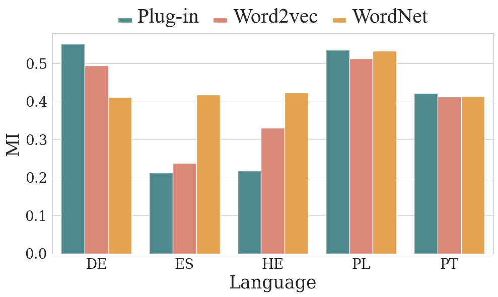
Figure 2: Results for the plug-in estimation of $\mathrm{MI}({\color[rgb]{0.5859375,0.16796875,0.375}{A}};{\color[rgb]{0.45703125,0.6171875,0.546875}{G}})$ and model-based estimations for $\mathrm{MI}({\color[rgb]{0.5859375,0.16796875,0.375}{A}};{\color[rgb]{0.45703125,0.6171875,0.546875}{G}})$.

6.6 Results

First, we validate our model by comparing the model-based estimation of $\mathrm{MI}({\color[rgb]{0.5859375,0.16796875,0.375}{A}};{\color[rgb]{0.45703125,0.6171875,0.546875}{G}})$ to the method presented in williams-etal-2021-relationships, the plug-in estimation of $\mathrm{MI}({\color[rgb]{0.5859375,0.16796875,0.375}{A}};{\color[rgb]{0.45703125,0.6171875,0.546875}{G}})$. Then, we employ our causal graphical model to investigate whether there is evidence for the neo-Whorfian claim that the grammatical gender of a noun influences the adjective choice to describe this noun, even when we control for the meaning of those nouns.

word2vec WordNet Model-based Model-based Mean diff. Model-based Model-based Mean diff. Lang $\mathrm{MI}({\color[rgb]{0.5859375,0.16796875,0.375}{A}};{\color[rgb]{0.45703125,0.6171875,0.546875}{G}})$ $\mathrm{MI}_{\mathrm{do}}({\color[rgb]{0.5859375,0.16796875,0.375}{A}};{\color[rgb]{0.45703125,0.6171875,0.546875}{G}})$ Perturbed $p$-value $\mathrm{MI}({\color[rgb]{0.5859375,0.16796875,0.375}{A}};{\color[rgb]{0.45703125,0.6171875,0.546875}{G}})$ $\mathrm{MI}_{\mathrm{do}}({\color[rgb]{0.5859375,0.16796875,0.375}{A}};{\color[rgb]{0.45703125,0.6171875,0.546875}{G}})$ Perturbed $p$-value de 0.526 ${1.24}\mathrm{e}{-4}$ ${2.84}\mathrm{e}{-4}$ 1.0 0.412 ${2.17}\mathrm{e}{-5}$ ${2.21}\mathrm{e}{-3}$ 1.0 es 0.238 ${4.60}\mathrm{e}{-5}$ ${3.05}\mathrm{e}{-4}$ 1.0 0.418 ${1.24}\mathrm{e}{-5}$ ${3.09}\mathrm{e}{-4}$ 1.0 he 0.331 ${8.03}\mathrm{e}{-4}$ ${6.93}\mathrm{e}{-4}$ 1.0 0.423 ${1.43}\mathrm{e}{-5}$ ${8.14}\mathrm{e}{-4}$ 1.0 pl 0.545 ${1.65}\mathrm{e}{-4}$ ${1.98}\mathrm{e}{-3}$ 1.0 0.533 ${8.68}\mathrm{e}{-7}$ ${3.33}\mathrm{e}{-3}$ 1.0 pt 0.413 ${1.72}\mathrm{e}{-4}$ ${1.06}\mathrm{e}{-3}$ 1.0 0.414 ${8.80}\mathrm{e}{-5}$ ${1.10}\mathrm{e}{-3}$ 1.0

Table 3: Results for the plug-in estimation of $\mathrm{MI}({\color[rgb]{0.5859375,0.16796875,0.375}{A}};{\color[rgb]{0.45703125,0.6171875,0.546875}{G}})$, model-based estimation for $\mathrm{MI}({\color[rgb]{0.5859375,0.16796875,0.375}{A}};{\color[rgb]{0.45703125,0.6171875,0.546875}{G}})$, and model-based estimation of $\mathrm{MI}_{\mathrm{do}}({\color[rgb]{0.5859375,0.16796875,0.375}{A}};{\color[rgb]{0.45703125,0.6171875,0.546875}{G}})$, mean difference between the model-based estimation of $\mathrm{MI}_{\mathrm{do}}({\color[rgb]{0.5859375,0.16796875,0.375}{A}};{\color[rgb]{0.45703125,0.6171875,0.546875}{G}})$ and a perturbed model with random gender labels together with permutation test results, and the $p$-values for the permutation test for the causal model trained with word2vec and WordNet representations.

We first validate our model by comparing its results to the williams-etal-2021-relationships plug-in estimate of $\mathrm{MI}({\color[rgb]{0.5859375,0.16796875,0.375}{A}};{\color[rgb]{0.45703125,0.6171875,0.546875}{G}})$. If the results of both of these estimates are comparable, we can assert that our model indeed captures the relation between grammatical gender and adjective choice. We present the results in Figure 2. We observe a substantial relationship between grammatical gender and adjective usage based on the plug-in and model-based $\mathrm{MI}({\color[rgb]{0.5859375,0.16796875,0.375}{A}};{\color[rgb]{0.45703125,0.6171875,0.546875}{G}})$ estimates replicating the results of williams-etal-2021-relationships. The estimates of the model-based $\mathrm{MI}({\color[rgb]{0.5859375,0.16796875,0.375}{A}};{\color[rgb]{0.45703125,0.6171875,0.546875}{G}})$ computed using both word2vec and WordNet representations, and the plug-in $\mathrm{MI}({\color[rgb]{0.5859375,0.16796875,0.375}{A}};{\color[rgb]{0.45703125,0.6171875,0.546875}{G}})$ lie between 0.2 and 0.5, with the estimates of the model-based approach being consistently higher (with the exception of German) than the estimates of the plug-in $\mathrm{MI}({\color[rgb]{0.5859375,0.16796875,0.375}{A}};{\color[rgb]{0.45703125,0.6171875,0.546875}{G}})$. Thus, the non-zero estimates of the model-based $\mathrm{MI}({\color[rgb]{0.5859375,0.16796875,0.375}{A}};{\color[rgb]{0.45703125,0.6171875,0.546875}{G}})$ indicate that some relationship exists between a noun’s grammatical gender and adjective usage.

Given the above result, we are interested in whether the strength of this relation is mitigated when controlling for the meaning of a noun. We present the estimates of the model-based $\mathrm{MI}_{\mathrm{do}}({\color[rgb]{0.5859375,0.16796875,0.375}{A}};{\color[rgb]{0.45703125,0.6171875,0.546875}{G}})$ in Tab 3 and compare them to the model-based estimates of the $\mathrm{MI}({\color[rgb]{0.5859375,0.16796875,0.375}{A}};{\color[rgb]{0.45703125,0.6171875,0.546875}{G}})$. While we observe evidence for the influence of grammatical gender on adjective choice in a non-causal setup based on $\mathrm{MI}({\color[rgb]{0.5859375,0.16796875,0.375}{A}};{\color[rgb]{0.45703125,0.6171875,0.546875}{G}})$, this relationship shrinks to close to 0 when we control for noun meaning in our causal model trained using both word2vec and WordNet representations. For completeness, we test for the presence of a difference between the size of the $\mathrm{MI}_{\mathrm{do}}({\color[rgb]{0.5859375,0.16796875,0.375}{A}};{\color[rgb]{0.45703125,0.6171875,0.546875}{G}})$ of our model and a model trained on randomly perturbed gender labels and find that we reject the null hypothesis that the distributions are exactly the same for all languages and representations’ settings.

6.7 Discussion

Evidence against the neo-Whorfian hypothesis.

We find that the interaction between the grammatical gender of inanimate nouns and the adjectives used to describe those nouns all but disappears when controlling for the meaning of those nouns, for all five analyzed gendered languages. The order of magnitude of $\mathrm{MI}_{\mathrm{do}}({\color[rgb]{0.5859375,0.16796875,0.375}{A}};{\color[rgb]{0.45703125,0.6171875,0.546875}{G}})$ measured with our model however significantly different from that of a model trained on random gender labels, is minuscule. This minor difference points towards the absence of a meaningful causal relationship between a noun’s gender and its descriptors in the languages studied. Thus, we provide an additional piece of evidence against the neo-Whorfian hypothesis.

A possible weakening of the neo-Whorfian hypothesis.

Although the size of the overall effect is small, it is possible that the effect of gender on adjective choice is stronger for some words than others. Future work could explore whether there is evidence of a noticeable effect of gender on adjective choice for a more restricted set of inanimate nouns, e.g., referring to artifacts or body parts. Such evidence could perhaps support a weakened version of the neo-Whorfian hypothesis.

Comparing results between word2vec and WordNet.

These results hold for both of the word representation setups, word2vec and WordNet. Notably, in comparing the two, we find that using WordNet representations consistently results in a lower $\mathrm{MI}_{\mathrm{do}}({\color[rgb]{0.5859375,0.16796875,0.375}{A}};{\color[rgb]{0.45703125,0.6171875,0.546875}{G}})$ than word2vec for all languages analyzed in this study. One possible explanation for this difference is that, despite our efforts to make non-contextual word2vec representations, these word2vec representations may still pick up some signal for gender from the remaining context (such as verb choice or adjacent gendered pronouns in the corpora). If these word2vec representations contain unwanted context-based gender information in addition to the noun meaning, it could result in overestimating $\mathrm{MI}_{\mathrm{do}}({\color[rgb]{0.5859375,0.16796875,0.375}{A}};{\color[rgb]{0.45703125,0.6171875,0.546875}{G}})$. Furthermore, since WordNet representations are created independently from any context within a corpus, they should not contain intruding grammatical gender signals, which may therefore be reflected in the consistently lower $\mathrm{MI}_{\mathrm{do}}({\color[rgb]{0.5859375,0.16796875,0.375}{A}};{\color[rgb]{0.45703125,0.6171875,0.546875}{G}})$.

Design choices and limitations.

We note several choices in the experimental setup which may influence this analysis. First, while we chose NorthEuraLex as a clean dataset to identify inanimate nouns, it excludes rarer nouns for which an effect might be observed. Second, while word embeddings are the current de facto representations for words in computational linguistics, they remain a proxy and are fundamentally limited. Furthermore, in our effort to learn word2vec representations for noun meaning without encoding gender-based context, we chose to remove some words in the context but not others. Specifically, while we remove adjectives which may carry signals of gender from the training corpora, we do not remove other parts of speech (e.g., verbs) under the reasoning that removing them may damage the training corpora too much for word2vec to effectively learn noun meanings. Future work can also explore improved representation methods for noun meaning. For example, recski2016measuring find that creating non-contextual word representations using a combination of word2vec, WordNet, and concept dictionaries can yield a better representation of meaning (i.e., achieving state-of-the-art correlation with the human-annotated similarity scores). Third, the corpus choice (and subsequently the noun–adjective pairs on which we conduct our analysis) may factor into the results. It is possible that when applied to other corpora (e.g., more colloquial ones like Reddit), this method may yield different results. Fourth, the choice of languages analyzed further limits this study to languages with up to three gender classes. Future work can investigate languages with more complex gender systems. Finally, our modeling approach assumes that the gender of a noun is influenced solely by its meaning. However, prior work has indicated that there are other factors that influence the grammatical gender of nouns such as their phonology and/or morphology (corbett1991gender). Therefore, future work should investigate more complex graphical models in order to account for other confounding factors.

6.8 Conclusion

In this paper, we introduce a causal graphical model which jointly represents the interactions between a noun’s grammatical gender, its meaning, and adjective choice. We employ our model on five languages that exhibit grammatical gender to investigate the influence of nouns’ gender on the adjectives chosen to describe those nouns. Replicating the findings of williams-etal-2021-relationships, we find a substantial correlation between grammatical gender and adjective choice. However, taking advantage of our causal perspective, we show that when controlling for a noun’s meaning, the effect of gender on adjective choice is marginal. Thus, we provide further evidence against the neo-Whorfian hypothesis.

6.9 Appendix

6.9.1 Proof of Proposition 1

See 1

Proof: First, define the following distribution $m({\color[rgb]{0.5859375,0.16796875,0.375}a})\overset{\text{\tiny def}}{=}\sum_{{\color[rgb]{0.45703125,0.6171875,0.546875}g}\in{\color[rgb]{0.45703125,0.6171875,0.546875}\mathcal{G}}}p_{{\color[rgb]{0.45703125,0.6171875,0.546875}{G}}}({\color[rgb]{0.45703125,0.6171875,0.546875}g})p({\color[rgb]{0.5859375,0.16796875,0.375}a}\mid\mathrm{do}({\color[rgb]{0.45703125,0.6171875,0.546875}{G}}={\color[rgb]{0.45703125,0.6171875,0.546875}g}))$. Now, the result follows by algebraic manipulation

$$\mathrm{JS}_{p_{{\color[rgb]{0.45703125,0.6171875,0.546875}{G}}}}\Big{(}\Big{\{}p(\cdot \mid\mathrm{do}({\color[rgb]{0.45703125,0.6171875,0.546875}{G}}={\color[rgb]{0.45703125,0.6171875,0.546875}g}))\Big{\}}\Big{)}=\sum_{{\color[rgb]{0.45703125,0.6171875,0.546875}g}\in{\color[rgb]{0.45703125,0.6171875,0.546875}\mathcal{G}}}p_{{\color[rgb]{0.45703125,0.6171875,0.546875}{G}}}({\color[rgb]{0.45703125,0.6171875,0.546875}g})\,\mathrm{KL}\Big{(}p(\cdot\mid\mathrm{do}({\color[rgb]{0.45703125,0.6171875,0.546875}{G}}={\color[rgb]{0.45703125,0.6171875,0.546875}g}))\mid\mid m\Big{)}$$ (6.10a)

$$=\sum_{{\color[rgb]{0.45703125,0.6171875,0.546875}g}\in{\color[rgb]{0.45703125,0.6171875,0.546875}\mathcal{G}}}p_{{\color[rgb]{0.45703125,0.6171875,0.546875}{G}}}({\color[rgb]{0.45703125,0.6171875,0.546875}g})\sum_{{\color[rgb]{0.5859375,0.16796875,0.375}a}\in{\color[rgb]{0.5859375,0.16796875,0.375}\mathcal{A}}}p({\color[rgb]{0.5859375,0.16796875,0.375}a}\mid\mathrm{do}({\color[rgb]{0.45703125,0.6171875,0.546875}{G}}={\color[rgb]{0.45703125,0.6171875,0.546875}g}))\Big{(}\log p({\color[rgb]{0.5859375,0.16796875,0.375}a}\mid\mathrm{do}({\color[rgb]{0.45703125,0.6171875,0.546875}{G}}={\color[rgb]{0.45703125,0.6171875,0.546875}g}))-\log m({\color[rgb]{0.5859375,0.16796875,0.375}a})\Big{)}$$ (6.10b)

$$=\!\begin{multlined}\sum_{{\color[rgb]{0.45703125,0.6171875,0.546875}g}\in{\color[rgb]{0.45703125,0.6171875,0.546875}\mathcal{G}}}p_{{\color[rgb]{0.45703125,0.6171875,0.546875}{G}}}({\color[rgb]{0.45703125,0.6171875,0.546875}g})\sum_{{\color[rgb]{0.5859375,0.16796875,0.375}a}\in{\color[rgb]{0.5859375,0.16796875,0.375}\mathcal{A}}}p({\color[rgb]{0.5859375,0.16796875,0.375}a}\mid\mathrm{do}({\color[rgb]{0.45703125,0.6171875,0.546875}{G}}={\color[rgb]{0.45703125,0.6171875,0.546875}g}))\log p({\color[rgb]{0.5859375,0.16796875,0.375}a}\mid\mathrm{do}({\color[rgb]{0.45703125,0.6171875,0.546875}{G}}={\color[rgb]{0.45703125,0.6171875,0.546875}g}))-\\ \sum_{{\color[rgb]{0.45703125,0.6171875,0.546875}g}\in{\color[rgb]{0.45703125,0.6171875,0.546875}\mathcal{G}}}p_{{\color[rgb]{0.45703125,0.6171875,0.546875}{G}}}({\color[rgb]{0.45703125,0.6171875,0.546875}g})\sum_{{\color[rgb]{0.5859375,0.16796875,0.375}a}\in{\color[rgb]{0.5859375,0.16796875,0.375}\mathcal{A}}}p({\color[rgb]{0.5859375,0.16796875,0.375}a}\mid\mathrm{do}({\color[rgb]{0.45703125,0.6171875,0.546875}{G}}={\color[rgb]{0.45703125,0.6171875,0.546875}g}))\log m({\color[rgb]{0.5859375,0.16796875,0.375}a})\end{multlined}\sum_{{\color[rgb]{0.45703125,0.6171875,0.546875}g}\in{\color[rgb]{0.45703125,0.6171875,0.546875}\mathcal{G}}}p_{{\color[rgb]{0.45703125,0.6171875,0.546875}{G}}}({\color[rgb]{0.45703125,0.6171875,0.546875}g})\sum_{{\color[rgb]{0.5859375,0.16796875,0.375}a}\in{\color[rgb]{0.5859375,0.16796875,0.375}\mathcal{A}}}p({\color[rgb]{0.5859375,0.16796875,0.375}a}\mid\mathrm{do}({\color[rgb]{0.45703125,0.6171875,0.546875}{G}}={\color[rgb]{0.45703125,0.6171875,0.546875}g}))\log p({\color[rgb]{0.5859375,0.16796875,0.375}a}\mid\mathrm{do}({\color[rgb]{0.45703125,0.6171875,0.546875}{G}}={\color[rgb]{0.45703125,0.6171875,0.546875}g}))-\\ \sum_{{\color[rgb]{0.45703125,0.6171875,0.546875}g}\in{\color[rgb]{0.45703125,0.6171875,0.546875}\mathcal{G}}}p_{{\color[rgb]{0.45703125,0.6171875,0.546875}{G}}}({\color[rgb]{0.45703125,0.6171875,0.546875}g})\sum_{{\color[rgb]{0.5859375,0.16796875,0.375}a}\in{\color[rgb]{0.5859375,0.16796875,0.375}\mathcal{A}}}p({\color[rgb]{0.5859375,0.16796875,0.375}a}\mid\mathrm{do}({\color[rgb]{0.45703125,0.6171875,0.546875}{G}}={\color[rgb]{0.45703125,0.6171875,0.546875}g}))\log m({\color[rgb]{0.5859375,0.16796875,0.375}a})$$ (6.10e)

$$=-\underbrace{\sum_{{\color[rgb]{0.45703125,0.6171875,0.546875}g}\in{\color[rgb]{0.45703125,0.6171875,0.546875}\mathcal{G}}}p_{{\color[rgb]{0.45703125,0.6171875,0.546875}{G}}}({\color[rgb]{0.45703125,0.6171875,0.546875}g})\mathrm{H}\left({\color[rgb]{0.5859375,0.16796875,0.375}{A}}\mid\mathrm{do}({\color[rgb]{0.45703125,0.6171875,0.546875}{G}}={\color[rgb]{0.45703125,0.6171875,0.546875}g}\right))}_{\overset{\text{\tiny def}}{=}\mathrm{H}_{\mathrm{do}}({\color[rgb]{0.5859375,0.16796875,0.375}{A}}\mid{\color[rgb]{0.45703125,0.6171875,0.546875}{G}})}-\sum_{{\color[rgb]{0.45703125,0.6171875,0.546875}g}\in{\color[rgb]{0.45703125,0.6171875,0.546875}\mathcal{G}}}p_{{\color[rgb]{0.45703125,0.6171875,0.546875}{G}}}({\color[rgb]{0.45703125,0.6171875,0.546875}g})\sum_{{\color[rgb]{0.5859375,0.16796875,0.375}a}\in{\color[rgb]{0.5859375,0.16796875,0.375}\mathcal{A}}}p({\color[rgb]{0.5859375,0.16796875,0.375}a}\mid\mathrm{do}({\color[rgb]{0.45703125,0.6171875,0.546875}{G}}={\color[rgb]{0.45703125,0.6171875,0.546875}g}))\log m({\color[rgb]{0.5859375,0.16796875,0.375}a})$$ (6.10f)

$$=-\mathrm{H}_{\mathrm{do}}\left({\color[rgb]{0.5859375,0.16796875,0.375}{A}}\mid{\color[rgb]{0.45703125,0.6171875,0.546875}{G}}\right)-\sum_{{\color[rgb]{0.45703125,0.6171875,0.546875}g}\in{\color[rgb]{0.45703125,0.6171875,0.546875}\mathcal{G}}}p_{{\color[rgb]{0.45703125,0.6171875,0.546875}{G}}}({\color[rgb]{0.45703125,0.6171875,0.546875}g})\sum_{{\color[rgb]{0.5859375,0.16796875,0.375}a}\in{\color[rgb]{0.5859375,0.16796875,0.375}\mathcal{A}}}p({\color[rgb]{0.5859375,0.16796875,0.375}a}\mid\mathrm{do}({\color[rgb]{0.45703125,0.6171875,0.546875}{G}}={\color[rgb]{0.45703125,0.6171875,0.546875}g}))\log m({\color[rgb]{0.5859375,0.16796875,0.375}a})$$ (6.10g)

$$=-\mathrm{H}_{\mathrm{do}}\left({\color[rgb]{0.5859375,0.16796875,0.375}{A}}\mid{\color[rgb]{0.45703125,0.6171875,0.546875}{G}}\right)-\sum_{{\color[rgb]{0.5859375,0.16796875,0.375}a}\in{\color[rgb]{0.5859375,0.16796875,0.375}\mathcal{A}}}\sum_{{\color[rgb]{0.45703125,0.6171875,0.546875}g}\in{\color[rgb]{0.45703125,0.6171875,0.546875}\mathcal{G}}}p_{{\color[rgb]{0.45703125,0.6171875,0.546875}{G}}}({\color[rgb]{0.45703125,0.6171875,0.546875}g})p({\color[rgb]{0.5859375,0.16796875,0.375}a}\mid\mathrm{do}({\color[rgb]{0.45703125,0.6171875,0.546875}{G}}={\color[rgb]{0.45703125,0.6171875,0.546875}g}))\log m({\color[rgb]{0.5859375,0.16796875,0.375}a})$$ (6.10h)

$$=-\mathrm{H}_{\mathrm{do}}\left({\color[rgb]{0.5859375,0.16796875,0.375}{A}}\mid{\color[rgb]{0.45703125,0.6171875,0.546875}{G}}\right)-\underbrace{\sum_{{\color[rgb]{0.5859375,0.16796875,0.375}a}\in{\color[rgb]{0.5859375,0.16796875,0.375}\mathcal{A}}}m({\color[rgb]{0.5859375,0.16796875,0.375}a})\log m({\color[rgb]{0.5859375,0.16796875,0.375}a})}_{\overset{\text{\tiny def}}{=}-\mathrm{H}_{\mathrm{do}}({\color[rgb]{0.5859375,0.16796875,0.375}{A}})}$$ (6.10i)

$$=-\mathrm{H}_{\mathrm{do}}\left({\color[rgb]{0.5859375,0.16796875,0.375}{A}}\mid{\color[rgb]{0.45703125,0.6171875,0.546875}{G}}\right)+\mathrm{H}_{\mathrm{do}}({\color[rgb]{0.5859375,0.16796875,0.375}{A}})=\mathrm{H}_{\mathrm{do}}({\color[rgb]{0.5859375,0.16796875,0.375}{A}})-\mathrm{H}_{\mathrm{do}}\left({\color[rgb]{0.5859375,0.16796875,0.375}{A}}\mid{\color[rgb]{0.45703125,0.6171875,0.546875}{G}}\right)=\mathrm{MI}_{\mathrm{do}}({\color[rgb]{0.5859375,0.16796875,0.375}{A}};{\color[rgb]{0.45703125,0.6171875,0.546875}{G}})$$ (6.10j)

$\blacksquare$

6.9.2 Data Statistics

	de	es	he	pl	pt
word2vec
# noun types	932	953	814	891	929
# adj types	109,549	61,839	29,855	42,271	30,004
# noun-adj types	486,647	581,589	208,202	223,774	176,995
# noun-adj tokens	5,966,400	7,523,601	2,413,546	4,040,464	1,543,563
WordNet
# noun types	437	773	391	450	630
# adj types	78,585	58,536	26,278	38,427	26,112
# noun-adj types	272,511	513,905	145,542	178,049	134,923
# noun-adj tokens	3,606,909	6,912,761	1,978,561	3,493,547	1,243,506

Table 4: Data statistics in our Wikipedia corpora with retrieved word2vec and WordNet representations.

Chapter 7 A Latent-Variable Model for Intrinsic Probing

The work presented in this chapter is based on a paper that has been published as:

stanczak2023latent.

Abstract

The success of pre-trained contextualized representations has prompted researchers to analyze them for the presence of linguistic information. Indeed, it is natural to assume that these pre-trained representations do encode some level of linguistic knowledge as they have brought about large empirical improvements on a wide variety of NLP tasks, which suggests they are learning true linguistic generalization. In this work, we focus on intrinsic probing, an analysis technique where the goal is not only to identify whether a representation encodes a linguistic attribute but also to pinpoint where this attribute is encoded. We propose a novel latent-variable formulation for constructing intrinsic probes and derive a tractable variational approximation to the log-likelihood. Our results show that our model is versatile and yields tighter mutual information estimates than two intrinsic probes previously proposed in the literature. Finally, we find empirical evidence that pre-trained representations develop a cross-lingually entangled notion of morphosyntax.

7.1 Introduction

There have been considerable improvements to the quality of pre-trained contextualized representations in recent years (e.g., peters-etal-2018-deep; devlin-etal-2019-bert; t5). These advances have sparked an interest in understanding what linguistic information may be lurking within the representations themselves (poliakCollectingDiverseNatural2018; zhang-bowman-2018-language; rogers-etal-2020-primer, inter alia). One philosophy that has been proposed to extract this information is called probing, the task of training an external classifier to predict the linguistic property of interest directly from the representations. The hope of probing is that it sheds light onto how much linguistic knowledge is present in representations and, perhaps, how that information is structured. Probing has grown to be a fruitful area of research, with researchers probing for morphological (tang-etal-2020-understanding-pure; acs-etal-2021-subword), syntactic (voita-titov-2020-information; hall-maudslay-etal-2020-tale; acs-etal-2021-subword), and semantic (vulic-etal-2020-probing; tang-etal-2020-understanding-pure) information.

In this paper, we focus on one type of probing known as intrinsic probing (dalviWhatOneGrain2019; torroba-hennigen-etal-2020-intrinsic), a subset of which specifically aims to ascertain how information is structured within a representation. This means that we are not solely interested in determining whether a network encodes the tense of a verb, but also in pinpointing exactly which neurons in the network are responsible for encoding the property. Unfortunately, the naïve formulation of intrinsic probing requires one to test all possible combinations of neurons, which is intractable even for the smallest representations used in modern-day NLP. For example, analyzing all combinations of 768-dimensional BERT representations would require training $2^{768}$ probes, one for each combination of neurons, which far exceeds the estimated number of atoms in the observable universe.

To obviate this difficulty, we introduce a novel latent-variable probe for intrinsic probing. Our core idea, instead of training a different probe for each subset of neurons, is to introduce a subset-valued latent variable. We approximately marginalize over the latent subsets using variational inference. Training the probe in this manner results in a set of parameters that work well across all possible subsets. We propose two variational families to model the posterior over the latent subset-valued random variables, both based on common sampling designs: Poisson sampling, which selects each neuron based on independent Bernoulli trials, and conditional Poisson sampling, which first samples a fixed number of neurons from a uniform distribution and then a subset of neurons of that size (lohr2019sampling). Conditional Poisson sampling offers the modeler more control over the distribution over subset sizes; they may pick the parametric distribution themselves.

We compare both variants to the two main intrinsic probing approaches we are aware of in the literature (§7.5). To do so, we train probes for 29 morphosyntactic properties across 6 languages from the Universal Dependencies (UD; ud-2.1) treebanks. We show that, in general, both variants of our method yield tighter estimates of the mutual information, though the model based on conditional Poisson sampling yields slightly better performance. This suggests that they are better at quantifying the informational content encoded in m-BERT representations (devlin-etal-2019-bert). We make two typological findings when applying our probe. We show that there is a difference in how information is structured depending on the language with certain language–attribute pairs requiring more dimensions to encode relevant information. We also analyze whether neural representations are able to learn cross-lingual abstractions from multilingual corpora. We confirm this statement and observe a strong overlap in the most informative dimensions, especially for number and gender. In an additional experiment, we show that our method supports training deeper probes (Section 7.8.2), though the advantages of non-linear probes over their linear counterparts are modest.

7.2 Intrinsic Probing

The success behind pre-trained contextual representations such as BERT (devlin-etal-2019-bert) suggests that they may offer a continuous analogue of the discrete structures in language, such as morphosyntactic attributes number, case, or tense. Intrinsic probing aims to recognize the parts of a network (assuming they exist) which encode such structures. In this paper, we operate exclusively at the level of the neuron—in the case of BERT, this is one component of the 768-dimensional vector the model outputs. However, our approach can easily generalize to other settings, e.g., the layers in a transformer or filters of a convolutional neural network. Identifying individual neurons responsible for encoding linguistic features of interest has previously been shown to increase model transparency (bauIdentifyingControllingImportant2019). In fact, knowledge about which neurons encode certain properties has also been employed to mitigate potential biases (vigInvestigatingGB2020), for controllable text generation (bauIdentifyingControllingImportant2019), and to analyze the linguistic capabilities of language models (lakretzEmergenceNumberSyntax2019).

To formally describe our intrinsic probing framework, we first introduce some notation. We define $\Pi$ to be the set of values that some property of interest can take, e.g., $\Pi=\{\textsc{Singular},\textsc{Plural}\}$ for the morphosyntactic number attribute. Let ${\mathcal{D}}=\{(\pi^{(n)},{\boldsymbol{h}}^{(n)})\}_{n=1}^{N}$ be a dataset of label–representation pairs: $\pi^{(n)}\in\Pi$ is a linguistic property and ${\boldsymbol{h}}^{(n)}\in\mathbb{R}^{d}$ is a representation. Additionally, let $D$ be the set of all neurons in a representation; in our setup, it is an integer range. In the case of BERT, we have $D=\{1,\ldots,768\}$. Given a subset of dimensions $C\subseteq D$, we write ${\boldsymbol{h}}_{C}$ for the subvector of ${\boldsymbol{h}}$ which contains only the dimensions present in $C$.

Let $p_{{\boldsymbol{\theta}}}({\pi}^{(n)}\mid{{\boldsymbol{h}}}^{(n)}_{C})$ be a probe—a classifier trained to predict ${\pi}^{(n)}$ from a subvector ${{\boldsymbol{h}}}^{(n)}_{C}$. In intrinsic probing, our goal is to find the size $k$ subset of neurons $C\subseteq D$ which are most informative about the property of interest. This may be written as the following combinatorial optimization problem (torroba-hennigen-etal-2020-intrinsic):

$$C^{\star}=\operatorname*{argmax}_{\begin{subarray}{c}C\subseteq D,\\ |C|=k\end{subarray}}\sum_{n=1}^{N}\log p_{{\boldsymbol{\theta}}}\left(\pi^{(n)}\mid{\boldsymbol{h}}^{(n)}_{C}\right)$$ (7.1)

To exhaustively solve Eq 7.1, we would have to train a probe $p_{{\boldsymbol{\theta}}}\left(\pi\mid{\boldsymbol{h}}_{C}\right)$ for every one of the exponentially many subsets $C\subseteq D$ of size $k$. Thus, exactly solving Eq. 7.1 is infeasible, and we are forced to rely on an approximate solution, e.g., greedily selecting the dimension that maximizes the objective. However, greedy selection alone is not enough to make solving Eq. 7.1 manageable; because we must retrain $p_{{\boldsymbol{\theta}}}\left(\pi\mid{\boldsymbol{h}}_{C}\right)$ for every subset $C\subseteq D$ considered during the greedy selection procedure, i.e., we would end up training $\mathcal{O}\left(k\,|D|\right)$ classifiers. As an example, consider what would happen if one used a greedy selection scheme to find the 50 most informative dimensions for a property on 768-dimensional BERT representations. To select the first dimension, one would need to train 768 probes. To select the second dimension, one would train an additional 767, and so forth. After 50 dimensions, one would have trained 37893 probes. To address this problem, our paper introduces a latent-variable probe, which identifies a ${\boldsymbol{\theta}}$ that can be used for any combination of neurons under consideration allowing a greedy selection procedure to work in practice.

7.3 A Latent-Variable Probe

The technical contribution of this work is a novel latent-variable model for intrinsic probing. Our method starts with a generic probabilistic probe $p_{{\boldsymbol{\theta}}}(\pi\mid C,{\boldsymbol{h}})$ which predicts a linguistic attribute $\pi$ given a subset $C$ of the hidden dimensions; $C$ is then used to subset ${\boldsymbol{h}}$ into ${{\boldsymbol{h}}_{C}}$. To avoid training a unique probe $p_{{\boldsymbol{\theta}}}(\pi\mid C,{\boldsymbol{h}})$ for every possible subset $C\subseteq D$, we propose to integrate a prior over subsets $p(C)$ into the model and then to marginalize out all possible subsets of neurons:

$$p_{{\boldsymbol{\theta}}}(\pi\mid{\boldsymbol{h}}) =\sum_{C\subseteq D}p_{{\boldsymbol{\theta}}}(\pi\mid C,{\boldsymbol{h}})\,p(C)$$ (7.2)

Due to this marginalization, our likelihood is not dependent on any specific subset of neurons $C$. Throughout this paper, we opted for a non-informative, uniform prior $p(C)$, but other distributions are also possible.

Our goal is to estimate the parameters ${\boldsymbol{\theta}}$. We achieve this by maximizing the log-likelihood of the training data $\sum_{n=1}^{N}\log\sum_{C\subseteq D}p_{{\boldsymbol{\theta}}}(\pi^{(n)},C\mid{{\boldsymbol{h}}}^{(n)})$ with respect to the parameters ${\boldsymbol{\theta}}$. Unfortunately, directly computing this involves a sum over all possible subsets of $D$—a sum with an exponential number of summands. Thus, we resort to a variational approximation. Let $q_{{\boldsymbol{\phi}}}(C)$ be a distribution over subsets, parameterized by parameters ${\boldsymbol{\phi}}$; we will use $q_{{\boldsymbol{\phi}}}(C)$ to approximate the true posterior distribution. Then, the log-likelihood is lower-bounded as follows:

$$\sum_{n=1}^{N}\log\sum_{C\subseteq D}p_{{\boldsymbol{\theta}}}(\pi^{(n)},C\mid{{\boldsymbol{h}}}^{(n)})$$ (7.3)

$$\geq\sum_{n=1}^{N}\left(\mathbb{E}_{q_{{\boldsymbol{\phi}}}}\left[\log p_{{\boldsymbol{\theta}}}({\pi}^{(n)},C\mid{{\boldsymbol{h}}}^{(n)})\right]+\mathrm{H}(q)\right)$$

which follows from Jensen’s inequality, where $\mathrm{H}(q_{{\boldsymbol{\phi}}})$ is the entropy of $q_{{\boldsymbol{\phi}}}$. The derivation of the variational lower bound is shown below:

$$\sum_{n=1}^{N}\log\sum_{C\subseteq D}p_{{\boldsymbol{\theta}}}(\pi^{(n)},C\mid{{\boldsymbol{h}}}^{(n)})$$ (7.4)

$$=\sum_{n=1}^{N}\log\sum_{C\subseteq D}q_{{\boldsymbol{\phi}}}(C)\frac{p_{{\boldsymbol{\theta}}}({\pi}^{(n)},C\mid{{\boldsymbol{h}}}^{(n)})}{q_{{\boldsymbol{\phi}}}(C)}$$

$$=\sum_{n=1}^{N}\log\mathbb{E}_{q_{{\boldsymbol{\phi}}}}\left[\frac{p_{{\boldsymbol{\theta}}}({\pi}^{(n)},C\mid{{\boldsymbol{h}}}^{(n)})}{q_{{\boldsymbol{\phi}}}(C)}\right]$$

$$\geq\sum_{n=1}^{N}\mathbb{E}_{q_{{\boldsymbol{\phi}}}}\left[\log\frac{p_{{\boldsymbol{\theta}}}({\pi}^{(n)},C\mid{{\boldsymbol{h}}}^{(n)})}{q_{{\boldsymbol{\phi}}}(C)}\right]$$ (7.5)

$$=\sum_{n=1}^{N}\left(\mathbb{E}_{q_{{\boldsymbol{\phi}}}}\left[\log p_{{\boldsymbol{\theta}}}({\pi}^{(n)},C\mid{{\boldsymbol{h}}}^{(n)})\right]+\mathrm{H}(q)\right)$$

Our likelihood is general and can take the form of any objective function. This means that we can use this approach to train intrinsic probes with any type of architecture amenable to gradient-based optimization, e.g., neural networks. However, in this paper, we use a linear classifier unless stated otherwise. Further, note that Eq. 7.3 is valid for any choice of $q_{{\boldsymbol{\phi}}}$. We explore two variational families for $q_{{\boldsymbol{\phi}}}$, each based on a common sampling technique. The first (herein Poisson) applies Poisson sampling (hajekAsymptoticTheoryRejective1964), which assumes each neuron to be subjected to an independent Bernoulli trial. The second one (Conditional Poisson; aires1999algorithms) corresponds to conditional Poisson sampling, which can be defined as conditioning a Poisson sample by a fixed sample size.

7.3.1 Parameter Estimation

As mentioned above, the exact computation of the log-likelihood is intractable due to the sum over all possible subsets of $D$. Thus, we optimize the variational bound presented in Eq. 7.3. We optimize the bound through stochastic gradient descent with respect to the model parameters ${\boldsymbol{\theta}}$ and the variational parameters ${\boldsymbol{\phi}}$, a technique known as stochastic variational inference (svi). However, one final trick is necessary, since the variational bound still includes a sum over all subsets in the first term:

$$\nabla_{{\boldsymbol{\theta}}}\mathbb{E}_{q_{{\boldsymbol{\phi}}}} \left[\log p_{{\boldsymbol{\theta}}}({\pi}^{(n)},C\mid{{\boldsymbol{h}}}^{(n)})\right]$$ (7.6)

$$\,\,=\mathbb{E}_{q_{{\boldsymbol{\phi}}}}\left[\nabla_{{\boldsymbol{\theta}}}\log p_{{\boldsymbol{\theta}}}({\pi}^{(n)},C\mid{{\boldsymbol{h}}}^{(n)})\right]$$

$$\,\,\approx\sum_{m=1}^{M}\left[\nabla_{{\boldsymbol{\theta}}}\log p_{{\boldsymbol{\theta}}}({\pi}^{(n)},C^{(m)}\mid{{\boldsymbol{h}}}^{(n)})\right]$$

where we take $M$ Monte Carlo samples to approximate the sum. In the case of the gradient with respect to ${\boldsymbol{\phi}}$, we also have to apply the REINFORCE trick  (Williams1992SimpleSG):

$$\nabla_{{\boldsymbol{\phi}}}\mathbb{E}_{q_{{\boldsymbol{\phi}}}}\left[\log p_{{\boldsymbol{\theta}}}({\pi}^{(n)},C\mid{{\boldsymbol{h}}}^{(n)})\right]$$ (7.7)

$$\,\,=\mathbb{E}_{q_{{\boldsymbol{\phi}}}}\left[\log p_{{\boldsymbol{\theta}}}({\pi}^{(n)},C\mid{{\boldsymbol{h}}}^{(n)})\nabla_{{\boldsymbol{\phi}}}\log q_{{\boldsymbol{\phi}}}(C)\right]$$

$$\,\,\approx\sum_{m=1}^{M}\left[\log p_{{\boldsymbol{\theta}}}({\pi}^{(n)},C^{(m)}\mid{{\boldsymbol{h}}}^{(n)})\nabla_{{\boldsymbol{\phi}}}\log q_{{\boldsymbol{\phi}}}(C)\right]$$

where we again take $M$ Monte Carlo samples. This procedure leads to an unbiased estimate of the gradient of the variational approximation.

7.3.2 Choice of Variational Family $q_{{\boldsymbol{\phi}}}(C)$.

We consider two choices of variational family $q_{{\boldsymbol{\phi}}}(C)$, both based on sampling designs lohr2019sampling. Each defines a parameterized distribution over all subsets of $D$.

Poisson Sampling.

Poisson sampling is one of the simplest sampling designs. In our setting, each neuron $d$ is given a unique non-negative weight $w_{d}=\exp(\phi_{d})$. This gives us the following parameterized distribution over subsets:

$$q_{{\boldsymbol{\phi}}}(C)=\prod_{d\in C}\frac{w_{d}}{1+w_{d}}\prod_{d\not\in C}\frac{1}{1+w_{d}}$$ (7.8)

The formulation in Eq. 7.8 shows that taking a sample corresponds to $|D|$ independent coin flips—one for each neuron—where the probability of heads is $\frac{w_{d}}{1+w_{d}}$. The entropy of a Poisson sampling may be computed in $\mathcal{O}\left(|D|\right)$ time:

$$\mathrm{H}(q_{{\boldsymbol{\phi}}})=\log Z-\sum_{d=1}^{\lvert D\rvert}\frac{w_{d}}{1+w_{d}}\log w_{d}$$ (7.9)

where $\log Z=\sum_{d=1}^{\lvert D\rvert}\log(1+w_{d})$. The gradient of Eq. 7.9 may be computed automatically through backpropagation. Poisson sampling automatically modules the size of the sampled set $C\sim q_{{\boldsymbol{\phi}}}(\cdot)$ and we have the expected size $\mathds{E}\left[|C|\right]=\sum_{d=1}^{|D|}\frac{w_{d}}{1+w_{d}}$.

Conditional Poisson Sampling.

We also consider a variational family that factors as follows:

$$q_{{\boldsymbol{\phi}}}(C)=\underbrace{q^{\mathrm{CP}}_{{\boldsymbol{\phi}}}(C\mid|C|=k)}_{\text{Conditional Poisson}}\,q^{\mathrm{size}}_{{\boldsymbol{\phi}}}(k)$$ (7.10)

In this paper, we take $q^{\mathrm{size}}_{{\boldsymbol{\phi}}}(k)=\mathrm{Uniform}\left(D\right)$, but a more complex distribution, e.g., a Categorical, could be learned. We define $q^{\mathrm{CP}}_{{\boldsymbol{\phi}}}(C\mid|C|=k)$ as a conditional Poisson sampling design. Similarly to Poisson sampling, conditional Poisson sampling starts with a unique positive weight associated with every neuron $w_{d}=\exp(\phi_{d})$. However, an additional cardinality constraint is introduced. This leads to the following distribution:

$$q^{\mathrm{CP}}_{{\boldsymbol{\phi}}}(C)=\mathds{1}\left\{|C|=k\right\}\frac{\prod_{d\in C}w_{d}}{Z^{\text{CP}}}$$ (7.11)

A more elaborate dynamic program which runs in $\mathcal{O}\left(k\,|D|\right)$ may be used to compute $Z^{\text{CP}}$ efficiently (aires1999algorithms). We may further compute the entropy $\mathrm{H}(q_{{\boldsymbol{\phi}}})$ and its the gradient in $\mathcal{O}\left(|D|^{2}\right)$ time using the expectation semiring eisner-2002-parameter; li-eisner-2009-first. Sampling from $q^{\mathrm{CP}}_{{\boldsymbol{\phi}}}$ can be done efficiently using quantities computed when running the dynamic program used to compute $Z^{\text{CP}}$ (Kulesza_2012).

7.4 Experimental Setup

Our setup is virtually identical to the morphosyntactic probing setup of torroba-hennigen-etal-2020-intrinsic. This consists of first automatically mapping treebanks from UD v2.1 (ud-2.1) to the UniMorph (mccarthyMarryingUniversalDependencies2018) schema. Then, we compute multilingual BERT (m-BERT) representations for every sentence in the UD treebanks. After computing the m-BERT representations for the entire sentence, we extract representations for individual words in the sentence and pair them with the UniMorph morphosyntactic annotations. We estimate our probes’ parameters using the UD training set and conduct greedy selection to approximate the objective in Eq. 7.1 on the validation set; finally, we report the results on the test set, i.e., we test whether the set of neurons we found on the development set generalizes to held-out data. Additionally, we discard values that occur fewer than 20 times across splits. When feeding ${{\boldsymbol{h}}_{C}}$ as input to our probes, we set any dimensions that are not present in $C$ to zero. We select $M=5$ as the number of Monte Carlo samples since we found this to work adequately in small-scale experiments. We compare the performance of the probes on 29 language–attribute pairs (listed in Section 7.8.1).

Since the performance of a probe on a specific subset of dimensions is related to both the subset itself (e.g., whether it is informative or not) and the number of dimensions being evaluated (e.g., if a probe is trained to expect 768 dimensions as input, it might work best when few or no dimensions are filled with zeros), we sample 100 subsets of dimensions with 5 different possible sizes (we considered 10, 50, 100, 250, 500 dim.) and compare every model’s performance on each of those subset sizes.

7.4.1 Baselines

We compare our latent-variable probe against two other recently proposed intrinsic probing methods as baselines.

• torroba-hennigen-etal-2020-intrinsic: Our first baseline is a generative probe that models the joint distribution of representations and their properties $p({\boldsymbol{h}},\pi)=p({\boldsymbol{h}}\mid\pi)\,p(\pi)$, where the representation distribution $p({\boldsymbol{h}}\mid\pi)$ is assumed to be Gaussian. torroba-hennigen-etal-2020-intrinsic report that a major limitation of this probe is that if certain dimensions of the representations are not distributed according to a Gaussian distribution, then probe performance will suffer.

• dalviWhatOneGrain2019: Our second baseline is a linear classifier, where dimensions not under consideration are zeroed out during evaluation (dalviWhatOneGrain2019; durrani-etal-2020-analyzing). Their approach is a special case of our proposed latent-variable model, where $q_{{\boldsymbol{\phi}}}$ is fixed so that on every training iteration the entire set of dimensions is sampled.

Additionally, we compare our methods to a naïve approach, a probe that is re-trained for every set of dimensions under consideration selecting the dimension that maximizes the objective (herein Upper Bound). Due to computational cost, we limit our comparisons with Upper Bound to 6 randomly chosen morphosyntactic attributes, each in a different language.

7.4.2 Metrics

We compare our proposed method to the baselines above under two metrics: accuracy and mutual information (MI). We report mutual information, which has recently been proposed as an evaluation metric for probes (pimentelInformationtheoreticProbingLinguistic2020). Here, mutual information (MI) is a function between a $\Pi$-valued random variable $P$ and a $\mathds{R}^{|C|}$-valued random variable $H_{C}$ over masked representations:

$$\mathrm{MI}(P;H_{C})=\mathrm{H}(P)-\mathrm{H}(P\mid H_{C})$$ (7.12)

where $\mathrm{H}(P)$ is the inherent entropy of the property being probed and is constant with respect to $H_{C}$; $\mathrm{H}(P\mid H_{C})$ is the entropy over the property given the representations $H_{C}$. Exact computation of the mutual information is intractable; however, we can lower-bound the MI by approximating $\mathrm{H}(P\mid H_{C})$ using our probe’s average negative log-likelihood: $-\frac{1}{N}\sum_{n=1}^{N}\log p_{{\boldsymbol{\theta}}}({\pi}^{(n)}\mid C,{{\boldsymbol{h}}}^{(n)})$ on held-out data. See brownEstimateUpperBound1992 for a derivation. We normalize the mutual information (NMI) by dividing the MI by the entropy which turns it into a percentage and is, arguably, more interpretable. We refer the reader to gatesElementcentricClusteringComparison2019 for a discussion of the normalization of MI.

We also report accuracy which is a standard measure for evaluating probes as it is for evaluating classifiers in general. However, accuracy can be a misleading measure, especially on imbalanced datasets since it considers solely correct predictions.

7.4.3 What Makes a Good Probe?

Since we report a lower bound on the mutual information (Section 7.4), we deem the best probe to be the one that yields the tightest mutual information estimate, or, in other words, the one that achieves the highest mutual information estimate; this is equivalent to having the best cross-entropy on held-out data, which is the standard evaluation metric for language modeling.

However, in the context of intrinsic probing, the topic of primary interest is what the probe reveals about the structure of the representations. For instance, does the probe reveal that the information encoded in the embeddings is focalized or dispersed across neurons? Several prior works (e.g., lakretzEmergenceNumberSyntax2019) focus on the single neuron setting, which is a special, very focal case. To engage with this work, we compare probes not only with respect to their performance (MI and accuracy), but also with respect to the size of the subset of dimensions being evaluated, i.e., the size of set $C$.

We acknowledge that there is a disparity between the quantitative evaluation we employ, in which probes are compared based on their MI estimates, and the qualitative nature of intrinsic probing, which aims to identify the substructures of a model that encode a property of interest. However, it is non-trivial to evaluate fundamentally qualitative procedures in a large-scale, systematic, and unbiased manner. Therefore, we rely on the quantitative evaluation metrics presented in Section 7.4.2, while also qualitatively inspecting the implications of our probes.

7.4.4 Training and Hyperparameter Tuning

We train our probes for a maximum of $2000$ epochs using the Adam optimizer (kingma15). We add early stopping with a patience of $50$ as a regularization technique. Early stopping is conducted by holding out 10% of the training data; our development set is reserved for the greedy selection of subsets of neurons. Our implementation is built with PyTorch (paszkePyTorchImperativeStyle2019). To execute a fair comparison with dalviWhatOneGrain2019, we train all probes other than the Gaussian probe using ElasticNet regularization (zouRegularizationVariableSelection2005), which consists of combining both $L_{1}$ and $L_{2}$ regularization, where the regularizers are weighted by tunable regularization coefficients $\lambda_{1}$ and $\lambda_{2}$, respectively. We follow the experimental set-up proposed by dalviWhatOneGrain2019, where we set $\lambda_{1},\lambda_{2}=10^{-5}$ for all probes. In a preliminary experiment, we performed a grid search over these hyperparameters to confirm that the probe is not very sensitive to the tuning of these values (unless they are extreme) which aligns with the claim presented in dalviWhatOneGrain2019. For Gaussian, we take the MAP estimate, with a weak data-dependent prior (murphyMachineLearningProbabilistic2012, Chapter 4). In addition, we found that a slight improvement in the performance of Poisson and Conditional Poisson was obtained by scaling the entropy term in Eq. 7.3 by a factor of $0.01$.

7.5 Results

In this section, we present the results of our empirical investigation. First, we address our main research question: Does our latent-variable probe presented in §7.3 outperform previously proposed intrinsic probing methods (§7.5.1)? Second, we analyze the structure of the most informative m-BERT neurons for the different morphosyntactic attributes we probe for (§7.5.2). Finally, we investigate whether knowledge about morphosyntax encoded in neural representations is shared across languages (§7.5.3). In Section 7.8.2, we show that our latent-variable probe is flexible enough to support deep neural probes.

7.5.1 How Do Our Methods Perform?

To investigate how the performance of our models compares to existing intrinsic probing approaches, we compare the performance of the Poisson and Conditional Poisson probes to Linear (dalviWhatOneGrain2019) and Gaussian (torroba-hennigen-etal-2020-intrinsic). We refer to Section 7.4.3 for a discussion of the limitations of our method.

	Number of dimensions
	$10$	$50$	$100$	$250$	$500$
	Gaussian
C. Poisson	0.50	0.58	0.70	0.99	1.00
Poisson	0.21	0.49	0.66	0.98	1.00
	Linear
C. Poisson	0.99	1.00	1.00	1.00	0.98
Poisson	0.95	0.99	1.00	1.00	0.97

Table 1: Proportion of experiments where Conditional Poisson (C. Poisson) and Poisson beat the benchmark models Linear and Gaussian in terms of NMI. For each of the subset sizes, we sampled 100 different subsets of BERT dimensions at random.

Probe	$10$	$50$	$100$	$250$	$500$	$768$
Cond. Poisson	$\mathbf{0.04\pm 0.03}$	$\mathbf{0.18\pm 0.10}$	$\mathbf{0.31\pm 0.14}$	$\mathbf{0.54\pm 0.17}$	$\mathbf{0.69\pm 0.15}$	$0.71\pm 0.15$
Poisson	$-0.18\pm 0.28$	$0.03\pm 0.24$	$0.22\pm 0.21$	$0.53\pm 0.17$	$\mathbf{0.69\pm 0.16}$	$0.71\pm 0.19$
Linear	$-0.28\pm 0.35$	$-0.18\pm 0.36$	$-0.06\pm 0.35$	$0.24\pm 0.33$	$0.59\pm 0.21$	$\mathbf{0.78\pm 0.14}$
Gaussian	$-0.15\pm 0.43$	$-1.20\pm 2.82$	$-3.97\pm 8.62$	$-61.70\pm 186.15$	$-413.80\pm 1175.31$	$-1067.08\pm 2420.08$
Cond. Poisson	$0.04\pm 0.03$	$0.21\pm 0.11$	$0.35\pm 0.16$	$0.58\pm 0.2$	$0.77\pm 0.19$	$0.74\pm 0.16$
Poisson	$-0.10\pm 0.10$	$0.11\pm 0.13$	$0.28\pm 0.17$	$0.57\pm 0.20$	$0.73\pm 0.20$	$0.76\pm 0.18$
Upper Bound	$\mathbf{0.10\pm 0.06}$	$\mathbf{0.36\pm 0.16}$	$\mathbf{0.52\pm 0.19}$	$\mathbf{0.70\pm 0.20}$	$\mathbf{0.79\pm 0.17}$	$\mathbf{0.81\pm 0.13}$

Table 2: Mean and standard deviation of NMI for the Conditional Poisson, Poisson, Linear (dalviWhatOneGrain2019) and Gaussian (torroba-hennigen-etal-2020-intrinsic) probes for all language–attribute pairs (top) and mean NMI and standard deviation for the Conditional Poisson, Poisson and Upper Bound for 6 selected language–attribute pairs (bottom). For each subset size considered, we take our averages over 100 randomly sampled subsets of BERT dimensions.

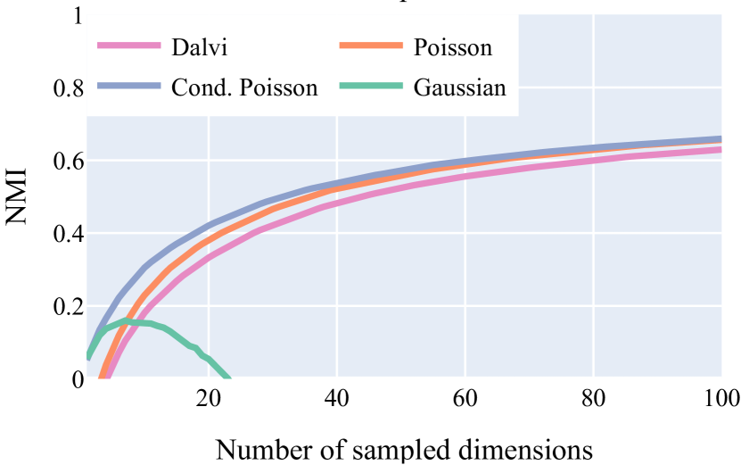
Figure 1: Comparison of NMI for the Poisson, Conditional Poisson, Linear (dalviWhatOneGrain2019) and Gaussian (torroba-hennigen-etal-2020-intrinsic) probes. We use the greedy selection approach in Eq 7.1 to select the most informative dimensions, and average across all language–attribute pairs we probe for.

In general, Conditional Poisson tends to outperform Poisson at lower dimensions, however, Poisson tends to catch up as more dimensions are added. Our results suggest that both variants of our latent-variable model from Section 7.3 are effective and generally outperform the Linear baseline as shown in Table 1. The Gaussian baseline tends to perform similarly to Conditional Poisson when we consider subsets of 10 dimensions, and it outperforms Poisson substantially. However, for subsets of size $50$ or more, both Conditional Poisson and Poisson are preferable. We believe that the robust performance of Gaussian in the low-dimensional regimen can be attributed to its ability to model non-linear decision boundaries (murphyMachineLearningProbabilistic2012, Chapter 4).

The trends above are corroborated by a comparison of the mean NMI (Table 2, top) achieved by each of these probes for different subset sizes. However, in terms of accuracy (see Table 4 in Section 7.8.3), while both Conditional Poisson and Poisson generally outperform Linear, Gaussian tends to achieve higher accuracy than our methods. Notwithstanding, Gaussian’s performance (in terms of NMI) is not stable and can yield low or even negative mutual information estimates across all subsets of dimensions. Adding a new dimension can never decrease the mutual information, so the observable decreases occur because the generative model deteriorates upon adding another dimension, which validates torroba-hennigen-etal-2020-intrinsic’s claim that some dimensions are not adequately modeled by the Gaussian assumption. While these results suggest that Gaussian may be preferable if performing a comparison based on accuracy, the instability of Gaussian when considering NMI suggests that this edge in terms of accuracy comes at a hefty cost in terms of calibration (guo2017calibration).

Further, we compare the Poisson and Conditional Poisson probes to the Upper Bound baseline. This is expected to be the highest performing since it is re-trained for every subset under consideration and indeed, this assumption is confirmed by the results in Table 2 (bottom). The difference between our probes’ performance and the Upper Bound baseline’s performance can be seen as the cost of sharing parameters across all subsets of dimensions, and an effective intrinsic probe should minimize this.

We also conduct a direct comparison of Linear, Gaussian, Poisson, and Conditional Poisson when used to identify the most informative subsets of dimensions. The average MI reported by each model across all 29 morphosyntactic language–attribute pairs is presented in Figure 1 (see Figure 4 in the Appendix for the accuracy comparison). On average, Conditional Poisson offers comparable performance to Gaussian at low dimensionalities for both NMI and accuracy, though the latter tends to yield a slightly higher (and thus a tighter) bound on the MI. However, as more dimensions are taken into consideration, our models vastly outperform Gaussian. Our models perform comparably at high dimensions, but Conditional Poisson performs slightly better for 1–20 dimensions. Poisson outperforms Linear at high dimensions, and Conditional Poisson outperforms Linear for all dimensions considered. These effects are less pronounced for accuracy, which we believe to be due to accuracy’s insensitivity to a probe’s confidence in its prediction. Finally, while Conditional Poisson achieves a tighter bound on NMI than Poisson, we recommend the Poisson probe for larger experimental setups due to its computational efficiency.

7.5.2 Information Distribution

We compare performance of the Conditional Poisson probe for each attribute for all available languages in order to better understand the relatively high NMI variance across results (see Table 2). In Figure 2, we plot the average NMI for gender and observe that languages with two genders present (Arabic and Portuguese) achieve higher performance than languages with three genders (Russian and Polish) which is an intuitive result due to increased task complexity. Further, we see that the slopes for both Russian and Polish are flatter, especially at lower dimensions. This implies that the information for Russian and Polish is more dispersed and more dimensions are needed to capture the typological information.

Figure 2: Comparison of the average NMI for gender dimensions in BERT for each of the available languages. We use the greedy selection approach in Eq 7.1 to select the most informative dimensions, and average across all language–attribute pairs we probe for.

7.5.3 Cross-Lingual Overlap

We compare the most informative m-BERT dimensions recovered by our probe across languages and find that, in many cases, the same set of neurons express the same morphosyntactic phenomena across languages. For example, we find that Russian, Polish, Portuguese, English, and Arabic have statistically significant overlap in the top 30 most informative neurons for number (Figure 3). Similarly, we observe presence of statistically significant overlap for gender (Figure 5, left). This effect is particularly strong between Russian and Polish, where we find statistically significant overlap between top-30 neurons for case (Figure 5, right). These results indicate that BERT may be leveraging data from other languages to develop a cross-lingually entangled notion of morpho-syntax (torroba-hennigen-etal-2020-intrinsic) and that this effect may be particularly strong between typologically similar languages.

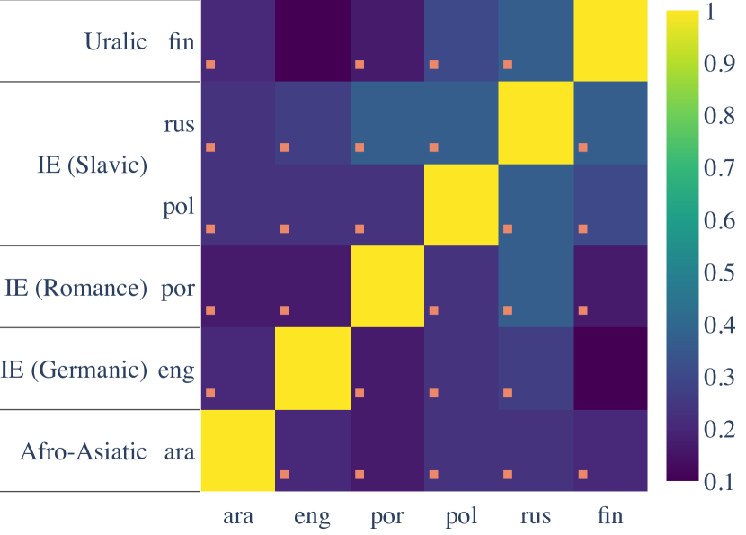
Figure 3: The percentage overlap between the top 30 most informative number dimensions in BERT for the probed languages. Statistically significant overlap, after Holm–Bonferroni family-wise error correction (holmSimpleSequentiallyRejective1979), with $\alpha=0.05$, is marked with an orange square.

7.6 Related Work

A growing interest in interpretability has led to a flurry of work in assessing what pre-trained representations know about language. To this end, diverse methods have been employed, such as the construction of challenge sets that evaluate how well representations model particular phenomena (linzenAssessingAbilityLSTMs2016; gulordavaColorlessGreenRecurrent2018; goldbergAssessingBERTSyntactic2019; goodwinProbingLinguisticSystematicity2020), and visualization methods (kadarFixed; RethmeierSA20). Work on probing comprises a major share of this endeavor (belinkovAnalysisMethodsNeural2019; belinkov2021probing). This has taken the form of focused studies on particular linguistic phenomena (e.g., subject-verb number agreement, giulianelliHoodUsingDiagnostic2018) to broad assessments of contextual representations in a wide array of tasks (sahinLINSPECTORMultilingualProbing2020; tenneyWhatYouLearn2018; conneauWhatYouCan2018; ravichander-etal-2021-probing; geva2022transformer, inter alia).

Efforts have ranged widely, but most of these focus on extrinsic rather than intrinsic probing. Most work on the latter has focused primarily on ascribing roles to individual neurons through methods such as visualization (karpathyVisualizingUnderstandingRecurrent2015; liVisualizingUnderstandingNeural2016) and ablation (liUnderstandingNeuralNetworks2017). For example, recently lakretzEmergenceNumberSyntax2019 conduct an in-depth study of how LSTMs (hochreiterLongShortTermMemory1997) capture subject–verb number agreement, and identify two units largely responsible for this phenomenon.

More recently, there has been a growing interest in extending intrinsic probing to collections of neurons. bauIdentifyingControllingImportant2019 utilize unsupervised methods to identify important neurons and then attempt to control a neural network’s outputs by selectively modifying them. bauUnderstandingRoleIndividual2020 pursue a similar goal in a computer vision setting but ascribe meaning to neurons based on how their activations correlate with particular classifications in images and are able to control these manually with interpretable results. Aiming to answer questions on interpretability in computer vision and natural language inference, mu2021compositional develop a method to create compositional explanations of individual neurons and investigate abstractions encoded in them. vigInvestigatingGB2020 analyze how information related to gender and societal biases is encoded in individual neurons and how it is being propagated through different model components.

7.7 Conclusion

In this paper, we introduce a new method for training intrinsic probes. We construct a probing classifier with a subset-valued latent variable and demonstrate how the latent subsets can be marginalized using variational inference. We propose two variational families, based on common sampling designs, to model the posterior over subsets: Poisson and conditional Poisson sampling. We demonstrate that both variants outperform our baselines in terms of mutual information and that using a conditional Poisson variational family generally gives optimal performance. Next, we investigate information distribution for each attribute for all available languages. Finally, we find empirical evidence for overlap in the specific neurons used to encode morphosyntactic properties across languages.

7.8 Appendix

7.8.1 List of Probed Morphosyntactic Attributes

The 29 language–attribute pairs we probe for in this work are listed below:

• Arabic: Aspect, Case, Definiteness, Gender, Mood, Number, Voice

• English: Number, Tense

• Finnish: Case, Number, Person, Tense, Voice

• Polish: Animacy, Case, Gender, Number, Tense

• Portuguese: Gender, Number, Tense

• Russian: Animacy, Aspect, Case, Gender, Number, Tense, Voice

7.8.2 How Do Deeper Probes Perform?

Multiple papers have promoted the use of linear probes (tenneyWhatYouLearn2018; liu-etal-2019-linguistic), in part because they are ostensibly less likely to memorize patterns in the data (zhang-bowman-2018-language; hewittDesigningInterpretingProbes2019), though this is subject to debate (voita-titov-2020-information; pimentelInformationtheoreticProbingLinguistic2020). Here we verify our claim from Section 7.3 that our probe can be applied to any kind of discriminative probe architecture as our objective function can be optimized using gradient descent.

We follow the setup of hewittDesigningInterpretingProbes2019, and test MLP-1 and MLP-2 Conditional Poisson probes alongside a linear Conditional Poisson probe. The MLP-1 and MLP-2 probes are multilayer perceptrons (MLP) with one and two hidden layer(s), respectively, and Rectified Linear Unit (ReLU; nairRectifiedLinearUnits2010) activation function.

In Table 3, we can see that our method not only works well for deeper probes but also outperforms the linear probe in terms of NMI. We note that the difference in performance between MLP-1 and MLP-2 is negligible.

7.8.3 Supplementary Results

Tab 4 compares the accuracy of our two models, Poisson and Conditional Poisson, to the Linear, Gaussian and Upper Bound baselines. The table reflects the trend observed in Table 2: Poisson and Conditional Poisson generally outperform the Linear baseline. However, Gaussian achieves higher accuracy with exception of a high-dimension regimen. In Figure 4, the accuracy reported by each model across all 29 morphosyntactic language–attribute pairs is presented.

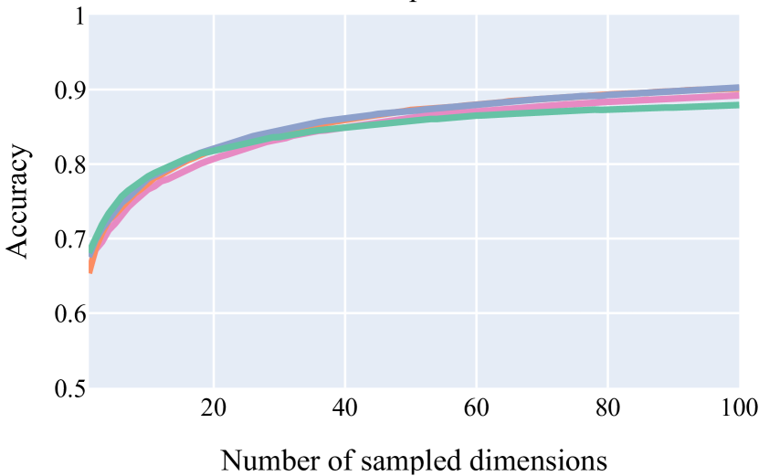
Figure 4: Comparison of the Poisson, Conditional Poisson, Linear (dalviWhatOneGrain2019) and Gaussian (torroba-hennigen-etal-2020-intrinsic) probes. We use the greedy selection approach in Eq 7.1 to select the most informative dimensions, and average across all language–attribute pairs we probe for.

Probe	$10$	$50$	$100$	$250$	$500$
Linear	$0.04\pm 0.03$	$0.21\pm 0.11$	$0.35\pm 0.15$	$0.59\pm 0.19$	$0.74\pm 0.18$
MLP-1	$\mathbf{0.06\pm 0.05}$	$0.26\pm 0.13$	$0.43\pm 0.16$	$0.67\pm 0.17$	$\mathbf{0.80\pm 0.14}$
MLP-2	$\mathbf{0.06\pm 0.05}$	$\mathbf{0.27\pm 0.13}$	$\mathbf{0.44\pm 0.17}$	$\mathbf{0.68\pm 0.17}$	$\mathbf{0.80\pm 0.14}$

Table 3: Mean and standard deviation of the NMI for the linear Conditional Poisson probe to non-linear MLP-1 and MLP-2 Conditional Poisson probes for selected language-attribute pairs. For each of the subset sizes, we sampled 100 different subsets of BERT dimensions at random.

Probe	$10$	$50$	$100$	$250$	$500$	$768$
Cond. Poisson	$0.66\pm 0.15$	$0.73\pm 0.13$	$0.78\pm 0.11$	$0.86\pm 0.08$	$\mathbf{0.92\pm 0.06}$	$0.93\pm 0.05$
Poisson	$0.62\pm 0.15$	$0.70\pm 0.13$	$0.77\pm 0.12$	$0.86\pm 0.08$	$\mathbf{0.92\pm 0.06}$	$0.94\pm 0.04$
Linear	$0.51\pm 0.15$	$0.59\pm 0.15$	$0.65\pm 0.14$	$0.77\pm 0.12$	$0.88\pm 0.08$	$\mathbf{0.95\pm 0.04}$
Gaussian	$\mathbf{0.69\pm 0.14}$	$\mathbf{0.80\pm 0.11}$	$\mathbf{0.84\pm 0.09}$	$\mathbf{0.88\pm 0.08}$	$0.88\pm 0.08$	$0.87\pm 0.1$
Cond. Poisson	$0.55\pm 0.1$	$0.65\pm 0.13$	$0.72\pm 0.12$	$0.83\pm 0.10$	$0.90\pm 0.08$	$0.93\pm 0.06$
Poisson	$0.51\pm 0.13$	$0.63\pm 0.14$	$0.72\pm 0.12$	$0.83\pm 0.10$	$0.90\pm 0.08$	$0.93\pm 0.07$
Upper Bound	$\mathbf{0.58\pm 0.12}$	$\mathbf{0.75\pm 0.12}$	$\mathbf{0.80\pm 0.10}$	$\mathbf{0.89\pm 0.08}$	$\mathbf{0.93\pm 0.06}$	$\mathbf{0.94\pm 0.05}$

Table 4: Mean and standard deviation of accuracy for the Poisson, Conditional Poisson, Linear (dalviWhatOneGrain2019) and Gaussian (torroba-hennigen-etal-2020-intrinsic) probes for all language–attribute pairs (above) and for the Conditional Poisson, Poisson and Upper Bound for 6 selected language–attribute pairs (below) for each of the subset sizes. We sampled 100 different subsets of BERT dimensions at random.

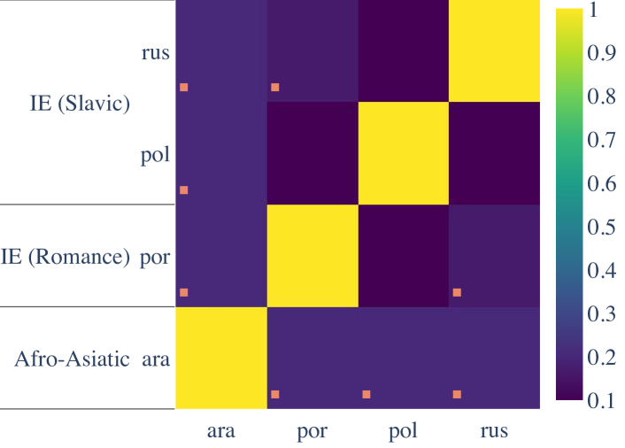
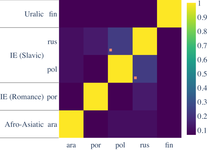
Figure 5: The percentage overlap between the top-30 most informative gender (left) and case (right) dimensions in BERT for the probed languages. Statistically significant overlap, after Holm–Bonferroni family-wise error correction (holmSimpleSequentiallyRejective1979), with $\alpha=0.05$, is marked with an orange square.

Chapter 8 Same Neurons, Different Languages: Probing Morphosyntax in Multilingual Pre-trained Models

The work presented in this chapter is based on a paper that has been published as:

stanczak-etal-2022-neuron.

Abstract

The success of multilingual pre-trained models is underpinned by their ability to learn representations shared by multiple languages even in absence of any explicit supervision. However, it remains unclear how these models learn to generalise across languages. In this work, we conjecture that multilingual pre-trained models can derive language-universal abstractions about grammar. In particular, we investigate whether morphosyntactic information is encoded in the same subset of neurons in different languages. We conduct the first large-scale empirical study over 43 languages and 14 morphosyntactic categories with a state-of-the-art neuron-level probe. Our findings show that the cross-lingual overlap between neurons is significant, but its extent may vary across categories and depends on language proximity and pre-training data size.

8.1 Introduction

Massively multilingual pre-trained models (devlin-etal-2019-bert; conneau-etal-2020-unsupervised; liu-etal-2020-multilingual-denoising; xue-etal-2021-mt5, inter alia) display an impressive ability to transfer knowledge between languages as well as to perform zero-shot learning (pires-etal-2019-multilingual; wu-dredze-2019-beto; nooralahzadeh-etal-2020-zero; hardalov2021fewshot, inter alia). Nevertheless, it remains unclear how pre-trained models actually manage to learn multilingual representations despite the lack of an explicit signal through parallel texts. Hitherto, many have speculated that the overlap of sub-words between cognates in related languages plays a key role in the process of multilingual generalisation (wu-dredze-2019-beto; Cao2020Multilingual; pires-etal-2019-multilingual; abendLexicalEventOrdering2015; vulic-etal-2020-probing).

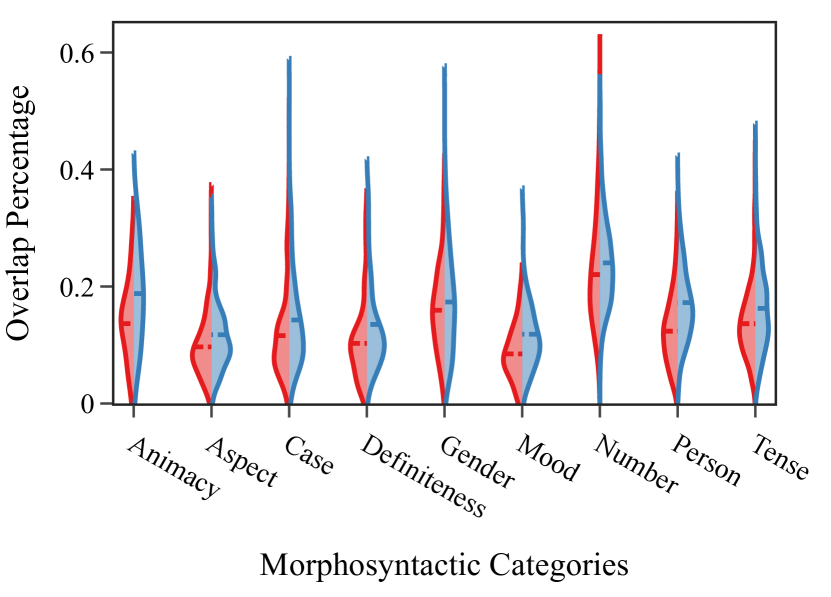
Figure 1: Percentages of neurons most associated with a particular morphosyntactic category that overlap between pairs of languages. Colours in the plot refer to 2 models: m-BERT (red) and XLM-R-base (blue).

In this work, we offer a concurrent hypothesis to explain the multilingual abilities of various pre-trained models; namely, that they implicitly align morphosyntactic markers that fulfil a similar grammatical function across languages, even in absence of any lexical overlap. More concretely, we conjecture that they employ the same subset of neurons to encode the same morphosyntactic information (such as gender for nouns and mood for verbs). To test the aforementioned hypothesis, we employ stanczak2023latent latent variable probe to identify the relevant subset of neurons in each language and then measure their cross-lingual overlap.

We experiment with two multilingual pre-trained models, m-BERT (devlin-etal-2019-bert) and XLM-R (conneau-etal-2020-unsupervised), probing them for morphosyntactic information in 43 languages from Universal Dependencies (ud-2.1). Based on our results, we argue that pre-trained models do indeed develop a cross-lingually entangled representation of morphosyntax. We further note that, as the number of values of a morphosyntactic category increases, cross-lingual alignment decreases. Finally, we find that language pairs with high proximity (in the same genus or with similar typological features) and with vast amounts of pre-training data tend to exhibit more overlap between neurons. Identical factors are known to affect also the empirical performance of zero-shot cross-lingual transfer (wu-dredze-2019-beto), which suggests a connection between neuron overlap and transfer abilities.

8.2 Intrinsic Probing

Intrinsic probing aims to determine exactly which dimensions in a representation, e.g., those given by m-BERT, encode a particular linguistic property (dalviWhatOneGrain2019; torroba-hennigen-etal-2020-intrinsic). Formally, let $\Pi$ be the inventory of values that some morphosyntactic category can take in a particular language, for example $\Pi=\{\textsc{fem},\textsc{msc},\textsc{neu}\}$ for grammatical gender in Russian. Moreover, let ${\mathcal{D}}=\{(\pi^{(n)},{\boldsymbol{h}}^{(n)})\}_{n=1}^{N}$ be a dataset of labelled embeddings such that $\pi^{(n)}\in\Pi$ and ${\boldsymbol{h}}^{(n)}\in\mathbb{R}^{d}$, where $d$ is the dimensionality of the representation being considered, e.g., $d=768$ for m-BERT. Our goal is to find a subset of $k$ neurons $C^{\star}\subseteq D=\{1,\ldots,d\}$, where $d$ is the total number of dimensions in the representation being probed, that maximises some informativeness measure.

In this paper, we make use of a latent-variable model recently proposed by stanczak2023latent for intrinsic probing. The idea is to train a probe with latent variable $C$ indexing the subset of the dimensions $D$ of the representation ${\boldsymbol{h}}$ that should be used to predict the property $\pi$:

$$p_{{\boldsymbol{\theta}}}(\pi\mid{\boldsymbol{h}}) =\sum_{C\subseteq D}p_{{\boldsymbol{\theta}}}(\pi\mid{\boldsymbol{h}},C)\,p(C)$$ (8.1)

where we opt for a uniform prior $p(C)$ and ${\boldsymbol{\theta}}$ are the parameters of the probe.

Our goal is to learn the parameters ${\boldsymbol{\theta}}$. However, since the computation of Eq. 8.1 requires us to marginalise over all subsets $C$ of $D$, which is intractable, we optimise a variational lower bound to the log-likelihood:

$$\mathcal{L} ({\boldsymbol{\theta}})=\sum_{n=1}^{N}\log\sum_{\begin{subarray}{c}C\subseteq D\end{subarray}}p_{\boldsymbol{\theta}}\left(\pi^{(n)},C\mid{\boldsymbol{h}}^{(n)}\right)\,$$ (8.2)

$$\geq\sum_{n=1}^{N}\left(\mathbb{E}_{q_{{\boldsymbol{\phi}}}}\left[\log p_{{\boldsymbol{\theta}}}(\pi^{(n)},C\mid{\boldsymbol{h}}^{(n)})\right]+\mathrm{H}(q_{{\boldsymbol{\phi}}})\right)$$

where $\mathrm{H}(\cdot)$ stands for the entropy of a distribution, and $q_{{\boldsymbol{\phi}}}(C)$ is a variational distribution over subsets $C$. For this paper, we chose $q_{{\boldsymbol{\phi}}}(\cdot)$ to correspond to a Poisson sampling scheme (lohr2019sampling), which models a subset as being sampled by subjecting each dimension to an independent Bernoulli trial, where $\phi_{i}$ parameterises the probability of sampling any given dimension.

Having trained the probe, all that remains is using it to identify the subset of dimensions that is most informative about the morphosyntactic category we are probing for. We do so by finding the subset $C^{\star}_{k}$ of $k$ neurons maximising the posterior:

$$C_{k}^{\star} =\operatorname*{argmax}_{\begin{subarray}{c}C\subseteq D,\\ |C|=k\end{subarray}}\log p_{{\boldsymbol{\theta}}}(C\mid{\mathcal{D}})$$ (8.3)

In practice, this combinatorial optimisation problem is intractable. Hence, we solve it using greedy search.

8.3 Experimental Setup

We now describe the experimental methodology of the paper, including the data, training procedure and statistical testing.

Data.

We select 43 treebanks from Universal Dependencies 2.1 (UD; ud-2.1), which contain sentences annotated with morphosyntactic information in a wide array of languages. Afterwards, we compute contextual representations for every individual word in the treebanks using multilingual BERT (m-BERT-base) and the base and large versions of XLM-RoBERTa (XLM-R-base and XLM-R-large). We then associate each word with its parts of speech and morphosyntactic features, which are mapped to the UniMorph schema (kirovUniMorphUniversalMorphology2018). The selected treebanks include all languages supported by both m-BERT and XLM-R which are available in UD.

Rather than adopting the default UD splits, we re-split word representations based on lemmata ending up with disjoint vocabularies for the train, development, and test set. This prevents a probe from achieving high performance by sheer memorising. Moreover, for every category–language pair (e.g., mood–Czech), we discard any lemma with fewer than 20 tokens in its split.

Training.

We first train a probe for each morphosyntactic category–language combination with the objective in Eq. 8.2. In line with established practices in probing, we parameterise $p_{{\boldsymbol{\theta}}}(\cdot)$ as a linear layer followed by a softmax. Afterwards, we identify the top-$k$ most informative neurons in the last layer of m-BERT, XLM-R-base, and XLM-R-large. Specifically, following torroba-hennigen-etal-2020-intrinsic, we use the log-likelihood of the probe on the test set as our greedy selection criterion. We single out 50 dimensions for each combination of morphosyntactic category and language.

Next, we measure the pairwise overlap in the top-$k$ most informative dimensions between all pairs of languages where a morphosyntactic category is expressed. This results in matrices such as Figure 2, where the pair-wise percentages of overlapping dimensions are visualised as a heat map.

Statistical Significance.

Suppose that two languages have $m\in\{1,\ldots,k\}$ overlapping neurons when considering the top-$k$ selected neurons for each of them. To determine whether such overlap is statistically significant, we compute the probability of an overlap of at least $m$ neurons under the null hypothesis that the sets of neurons are sampled independently at random. We estimate these probabilities with a permutation test. In this paper, we set a threshold of $\alpha=0.05$ for significance.

Family-wise Error Correction.

Finally, we use Holm-Bonferroni (holmSimpleSequentiallyRejective1979) family-wise error correction. Hence, our threshold is appropriately adjusted for multiple comparisons, which makes incorrectly rejecting the null hypothesis less likely.

In particular, the individual permutation tests are ordered in ascending order of their $p$-values. The test with the smallest probability undergoes the Holm–Bonferroni correction (holmSimpleSequentiallyRejective1979). If already the first test is not significant, the procedure stops; otherwise, the test with the second smallest $p$-value is corrected for a family of $t-1$ tests, where $t$ denotes the number of conducted tests. The procedure stops either at the first non-significant test or after iterating through all $p$-values. This sequential approach guarantees that the probability that we incorrectly reject one or more of the hypotheses is at most $\alpha$.

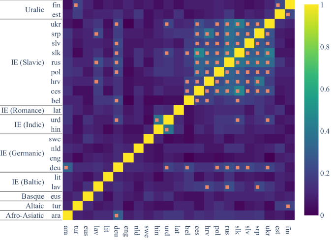
Figure 2: The percentage overlap between the top-50 most informative number dimensions in m-BERT for number (top) and XLM-R-large for case (bottom). Statistically significant overlap after Holm–Bonferroni family-wise error correction (holmSimpleSequentiallyRejective1979), with $\alpha=0.05$, is marked with an orange square.

8.4 Results

We first consider whether multilingual pre-trained models develop a cross-lingually entangled notion of morphosyntax: for this purpose, we measure the overlap between subsets of neurons encoding similar morphosyntactic categories across languages. Further, we debate whether the observed patterns are dependent on various factors, such as morphosyntactic category, language proximity, pre-trained model, and pre-training data size.

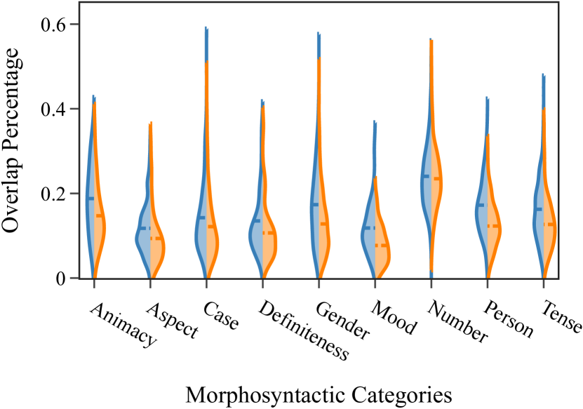
Figure 3: Ratio of neurons most associated with a particular morphosyntactic category that overlap between pairs of languages. Colours in the plot refer to 2 models: XLM-R-base (blue) and XLM-R-large (orange).

Neuron Overlap.

The matrices of pairwise overlaps for each of the 14 categories, such as Figure 2 for number and case, are reported in Section 8.6.2. We expand upon these results in two ways. First, we report the cross-lingual distribution for each category in Figure 1 for m-BERT and XLM-R-base, and in an equivalent plot comparing XLM-R-base and XLM-R-large in Figure 3. Second, we calculate how many overlaps are statistically significant out of the total number of pairwise comparisons in Table 1. From the above results, it emerges that $\approx 20$% of neurons among the top-$50$ most informative ones overlap on average, but this number may vary dramatically across categories.

	m-BERT	XLM-R-base	XLM-R-large	Total
Definiteness	0.11	0.22	0.13	45
Comparison	0.20	0.90	0.50	10
Possession	0.00	0.00	0.00	1
Aspect	0.03	0.10	0.09	153
Polarity	0.33	0.67	0.33	3
Number	0.40	0.51	0.74	666
Animacy	0.14	0.57	0.32	28
Mood	0.00	0.07	0.05	105
Gender	0.15	0.32	0.19	378
Person	0.08	0.25	0.13	276
POS	0.04	0.27	0.70	861
Case	0.10	0.18	0.17	300
Tense	0.08	0.23	0.12	325
Finiteness	0.09	0.18	0.09	45

Table 1: Proportion of language pairs with statistically significant overlap in the top-50 neurons for an attribute (after Holm–Bonferroni (holmSimpleSequentiallyRejective1979) correction). We compute these ratios for each model. The final column reports the total number of pairwise comparisons.

Morphosyntactic Categories.

Based on Table 1, significant overlap is particularly accentuated in specific categories, such as comparison, polarity, and number. However, neurons for other categories such as mood, aspect, and case are shared by only a handful of language pairs despite the high number of comparisons. This finding may be partially explained by the different number of values each category can take. Hence, we test whether there is a correlation between this number and average cross-lingual overlap in Figure 8.5(a). As expected, we generally find negative correlation coefficients—prominent exceptions being number and person. As the inventory of values of a category grows, cross-lingual alignment becomes harder.

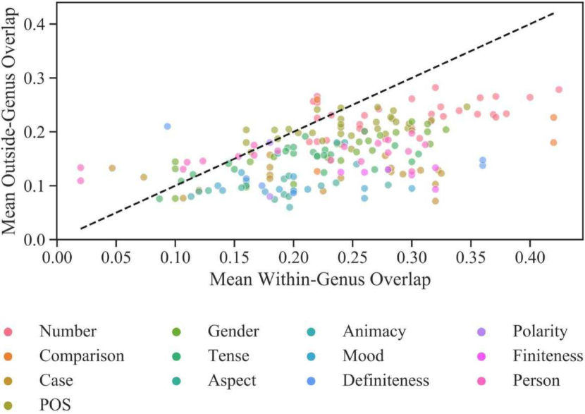
Figure 4: Mean percentage of neuron overlap in XLM-R-base with languages either within or outside the same genus for each morphosyntactic category.

Figure 5: Spearman’s correlation, for a given model and morphological category, between the cross-lingual average percentage of overlapping neurons and:

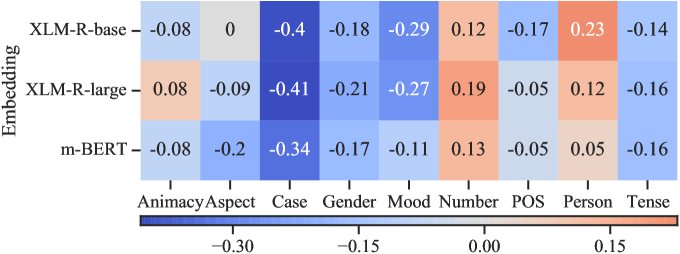
(a) number of values for each morphosyntactic category;

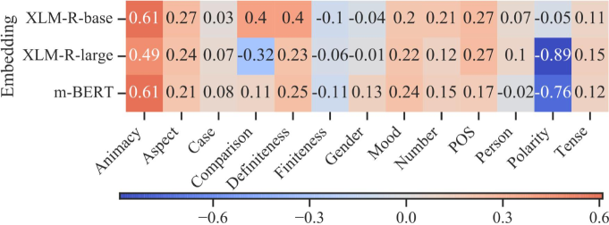
(b) typological similarity;

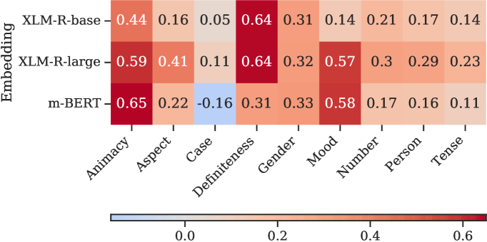
(c) language model training data size.

Language Proximity.

Moreover, we investigate whether language proximity, in terms of both language family and typological features, bears any relationship with the neuron overlap for any particular pair. In Figure 4, we plot pairwise similarities with languages within the same genus (e.g., Baltic) against those outside. From the distribution of the dots, we can extrapolate that sharing of neurons is more likely to occur between languages in the same genus. This is further corroborated by the language groupings emerging in the matrices of Section 8.6.2.

In Figure 8.5(b), we also measure the correlation between neuron overlap and similarity of syntactic typological features based on littell2017uriel. While correlation coefficients are mostly positive (with the exception of polarity), we remark that the patterns are strongly influenced by whether a category is typical for a specific genus. For instance, correlation is highest for animacy, a category almost exclusive to Slavic languages in our sample.

Pre-trained Models.

Afterwards, we determine whether the 3 models under consideration reveal different patterns. Comparing m-BERT and XLM-R-base in Figure 1, we find that, on average, XLM-R-base tends to share more neurons when encoding particular morphosyntactic attributes. Moreover, comparing XLM-R-base to XLM-R-large in Figure 3 suggests that more neurons are shared in the former than in the latter.

Altogether, these results seem to suggest that the presence of additional training data engenders cross-lingual entanglement, but increasing model size incentivises morphosyntactic information to be allocated to different subsets of neurons. We conjecture that this may be best viewed from the lens of compression: if model size is a bottleneck, then, to attain good performance across many languages, a model is forced to learn cross-lingual abstractions that can be reused.

Pre-training Data Size.

Finally, we assess the effect of pre-training data size for neuron overlap. According to Figure 8.5(c), their correlation is very high. We explain this phenomenon with the fact that more data yields higher-quality (and as a consequence, more entangled) multilingual representations.

8.5 Conclusions

In this paper, we hypothesise that the ability of multilingual models to generalise across languages results from cross-lingually entangled representations, where the same subsets of neurons encode universal morphosyntactic information. We validate this claim with a large-scale empirical study on 43 languages and 3 models, m-BERT, XLM-R-base, and XLM-R-large. We conclude that the overlap is statistically significant for a notable amount of language pairs for the considered attributes. However, the extent of the overlap varies across morphosyntactic categories and tends to be lower for categories with large inventories of possible values. Moreover, we find that neuron subsets are shared mostly between languages in the same genus or with similar typological features. Finally, we discover that the overlap of each language grows proportionally to its pre-training data size, but it also decreases in larger model architectures.

Given that this implicit morphosyntactic alignment may affect the transfer capabilities of pre-trained models, we speculate that, in future work, artificially encouraging a tighter neuron overlap might facilitate zero-shot cross-lingual inference to low-resource and typologically distant languages(zhao-etal-2021-inducing).

Ethics Statement

The authors foresee no ethical concerns with the work presented in this paper.

Acknowledgments

This work is mostly funded by Independent Research Fund Denmark under grant agreement number 9130-00092B, as well as by a project grant from the Swedish Research Council under grant agreement number 2019-04129. Lucas Torroba Hennigen acknowledges funding from the Michael Athans Fellowship fund. Ryan Cotterell acknowledges support from the Swiss National Science Foundation (SNSF) as part of the “The Forgotten Role of Inductive Bias in Interpretability” project.

8.6 Appendix

8.6.1 Probed Property–Language Pairs

Afro-Asiatic

• ara (Arabic): Gender, Voice, Mood, Part of Speech, Aspect, Person, Number, Case, Definiteness

• heb (Hebrew): Part of Speech, Number, Tense, Person, Voice

Austroasiatic

• vie (Vietnamese): Part of Speech

Dravidian

• tam (Tamil): Part of Speech, Number, Gender, Case, Person, Finiteness, Tense

Indo-European

• afr (Afrikaans): Part of Speech, Number, Tense

• bel (Berlarusian): Part of Speech, Tense, Number, Aspect, Finiteness, Voice, Gender, Animacy, Case, Person

• bul (Bulgarian): Part of Speech, Definiteness, Gender, Number, Mood, Tense, Person, Voice, Comparison

• cat (Catalan): Gender, Number, Part of Speech, Tense, Mood, Person, Aspect

• ces (Czech): Part of Speech, Number, Case, Comparison, Gender, Mood, Person, Tense, Aspect, Polarity, Animacy, Possession, Voice

• dan (Danish): Part of Speech, Number, Gender, Definiteness, Voice, Tense, Mood, Comparison

• deu (German): Part of Speech, Case, Number, Tense, Person, Comparison

• ell (Greek): Part of Speech, Case, Gender, Number, Finiteness, Person, Tense, Aspect, Mood, Voice, Comparison

• eng (English): Part of Speech, Number, Tense, Case, Comparison

• fas (Persian): Number, Part of Speech, Tense, Person, Mood, Comparison

• fra (French): Part of Speech, Number, Gender, Tense, Mood, Person, Polarity, Aspect

• gle (Irish): Tense, Mood, Part of Speech, Number, Person, Gender, Case

• glg (Galician): Part of Speech

• hin (Hindi): Person, Case, Part of Speech, Number, Gender, Voice, Aspect, Mood, Finiteness, Politeness

• hrv (Croatian): Case, Gender, Number, Part of Speech, Person, Finiteness, Mood, Tense, Animacy, Definiteness, Comparison, Voice

• ita (Italian): Part of Speech, Number, Gender, Person, Mood, Tense, Aspect

• lat (Latin): Part of Speech, Number, Gender, Case, Tense, Person, Mood, Aspect, Comparison

• lav (Latvian): Part of Speech, Case, Number, Tense, Mood, Person, Gender, Definiteness, Aspect, Comparison, Voice

• lit (Lithuanian): Tense, Voice, Number, Part of Speech, Finiteness, Mood, Polarity, Person, Gender, Case, Definiteness

• mar (Marathi): Case, Gender, Number, Part of Speech, Person, Aspect, Tense, Finiteness

• nld (Dutch): Person, Part of Speech, Number, Gender, Finiteness, Tense, Case, Comparison

• pol (Polish): Part of Speech, Case, Number, Animacy, Gender, Aspect, Tense, Person, Polarity, Voice

• por (Portuguese): Part of Speech, Person, Mood, Number, Tense, Gender, Aspect

• ron (Romanian): Definiteness, Number, Part of Speech, Person, Aspect, Mood, Case, Gender, Tense

• rus (Russian): Part of Speech, Case, Gender, Number, Animacy, Tense, Finiteness, Aspect, Person, Voice, Comparison

• slk (Slovak): Part of Speech, Gender, Case, Number, Aspect, Polarity, Tense, Voice, Animacy, Finiteness, Person, Mood, Comparison

• slv (Slovenian): Number, Gender, Part of Speech, Case, Mood, Person, Finiteness, Aspect, Animacy, Definiteness, Comparison

• spa (Spanish): Part of Speech, Tense, Aspect, Mood, Number, Person, Gender

• srp (Serbian): Number, Part of Speech, Gender, Case, Person, Tense, Definiteness, Animacy, Comparison

• swe (Swedish): Part of Speech, Gender, Number, Definiteness, Case, Tense, Mood, Voice, Comparison

• ukr (Ukrainian): Case, Number, Part of Speech, Gender, Tense, Animacy, Person, Aspect, Voice, Comparison

• urd (Urdu): Case, Number, Part of Speech, Person, Finiteness, Voice, Mood, Politeness, Aspect

Japonic

• jpn (Japanese): Part of Speech

Language isolate

• eus (Basque): Part of Speech, Case, Animacy, Definiteness, Number, Argument Marking, Aspect, Comparison

Sino-Tibetan

• zho (Chinese): Part of Speech

Turkic

• tur (Turkish): Case, Number, Part of Speech, Aspect, Person, Mood, Tense, Polarity, Possession, Politeness

Uralic

• est (Estonian): Part of Speech, Mood, Finiteness, Tense, Voice, Number, Person, Case

• fin (Finnish): Part of Speech, Case, Number, Mood, Person, Voice, Tense, Possession, Comparison

8.6.2 Pairwise Overlap by Morphosyntactic Category

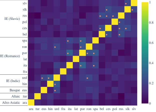
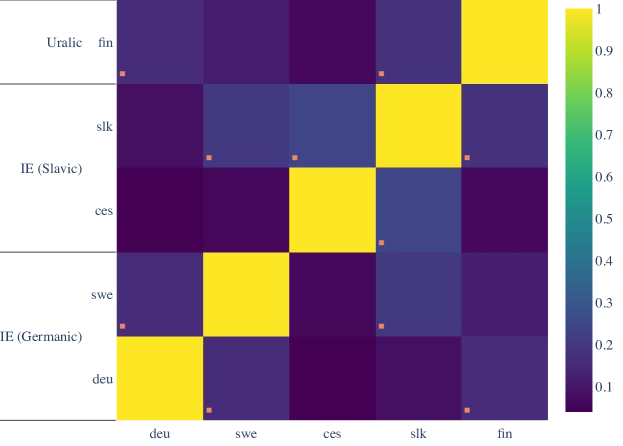
(a) Aspect–XLM-R-base

(b) Comparison–XLM-R-large

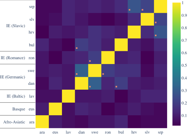
(a) Definiteness–m-BERT

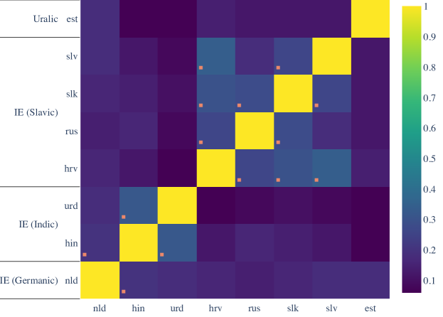
(b) Finiteness–XLM-R-base

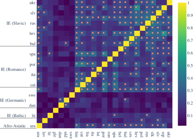
(a) Gender–XLM-R-base

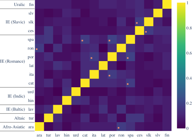
(b) Mood–XLM-R-large

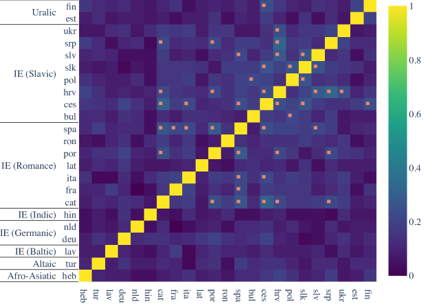
(a) Person–m-BERT

(b) Polarity–XLM-R-large

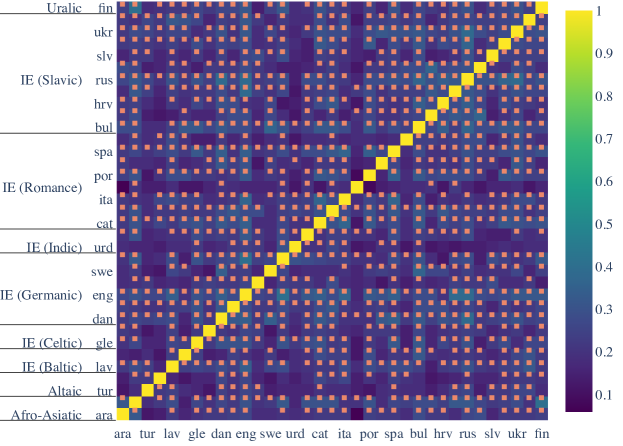
(a) Part of Speech–XLM-R-large

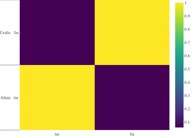
(b) Possession–XLM-R-base

(a) Tense–XLM-R-base

Chapter 9 Quantifying Gender Bias Towards Politicians in Cross-Lingual Language Models

The work presented in this chapter is based on a paper that has been published as:

stanczak2021quantifying.

Abstract

Recent research has demonstrated that large pre-trained language models reflect societal biases expressed in natural language. The present paper introduces a simple method for probing language models to conduct a multilingual study of gender bias towards politicians. We quantify the usage of adjectives and verbs generated by language models surrounding the names of politicians as a function of their gender. To this end, we curate a dataset of 250k politicians worldwide, including their names and gender. Our study is conducted in seven languages across six different language modeling architectures. The results demonstrate that pre-trained language models’ stance towards politicians varies strongly across analyzed languages. We find that while some words such as dead, and designated are associated with both male and female politicians, a few specific words such as beautiful and divorced are predominantly associated with female politicians. Finally, and contrary to previous findings, our study suggests that larger language models do not tend to be significantly more gender-biased than smaller ones.

9.1 Introduction

In the last decades, digital media has become a primary source of information about political discourse (kleinberg2019) with a dominant share of discussions occurring online (keith2017social). The Internet and social media especially are able to shape public sentiment towards politicians (zhuravskaya2020), which, in an extreme case, can influence election results (mohammad15sentiment), and, thus, the composition of a country’s government (metaxas2012). However, information presented online is subjective, biased, and potentially harmful as it may disseminate misinformation and toxicity. For instance, prabhakaran-etal-2019-perturbation show that online comments about politicians, in particular, tend to be more toxic than comments about people in other occupations.

Relatedly, natural language processing (NLP) models are increasingly being used across various domains of the Internet (e.g., in search) (Huang2013LearningDS) and social media (e.g., to translate posts) (gotti-etal-2013-translating). These models, however, are typically trained on subjective and imbalanced data. Thus, while they appear to successfully learn general formal properties of the language (e.g., syntax, semantics (liu-etal-2019-linguistic; rogers-etal-2020-primer)), they are also susceptible to learning potentially harmful associations (prabhakaran-etal-2019-perturbation). In particular, pre-trained language models are shown to perpetuate and amplify societal biases found in their training data (bender-etal-2021-dangers). For instance, shwartz-etal-2020-grounded showed that pre-trained language models associated negativity with a certain name if the name corresponded to an entity who was frequently mentioned in negative contexts (e.g., Donald for Donald Trump). This strongly suggests a risk of harm when employing language models on downstream tasks such as search or translation.

One such harm that a language model could propagate is that of gender bias (basta-etal-2019-evaluating). In fact, pre-trained language models have been reported to encode gender bias and stereotypes (bender-etal-2021-dangers; nadeem-etal-2021-stereoset; nangia-etal-2020-crows). Most previous work examining gender bias in language models has focused on English (stanczak-etal-2021-survey), with only a few notable exceptions in recent years (liang-etal-2020-monolingual; kaneko-etal-2022-gender; neveol-etal-2022-french; martinkova-etal-2023-measuring). The approaches taken in prior work have relied on a range of methods including causal analysis (vig2020causal), statistical measures such as association tests (may-etal-2019-measuring; nadeem-etal-2021-stereoset), and correlations (webster2020measuring). Their findings indicate that gender biases that exist in natural language corpora are also reflected in the text generated by language models.

Gender bias has been examined in stance analysis approaches, but with most investigations focusing on natural language corpora as opposed to language models. For instance, ahmad-etal-2011-new and voigt-etal-2018-rtgender explicitly controlled for gender bias in two small-scale natural language corpora that focused on politicians within a single country. Specifically, according to ahmad-etal-2011-new the media coverage given to male and female candidates in Irish elections did not correspond to the ratio of male to female contestants, with male candidates receiving more coverage. Perhaps surprisingly, voigt-etal-2018-rtgender found that there is a smaller difference in the sentiment of responses written to male and female politicians, as opposed to other public figures. However, it is unclear whether these findings would generalize when tested at scale (i.e., examining political figures from around the world) and in text generated by language models.

In this paper, we present a large-scale study on quantifying gender bias in language models with a focus on stance towards politicians. To this end, we generate a dataset for analyzing stance towards politicians encoded in a language model, where stance is inferred from simple grammatical constructs (e.g., “$\langle\textsc{blank}\rangle$ person” where $\langle\textsc{blank}\rangle$ is an adjective or a verb). Moreover, we make use of a statistical method to measure gender bias – namely, a latent-variable model – and adapt this to language models. Further, while prior work has focused on monolingual language models (webster2020measuring; nadeem-etal-2021-stereoset), we present a fine-grained study of gender bias in six multilingual language models across seven languages, considering 250k politicians from the majority of the world’s countries.

In our experiments, we find that, for both male and female politicians, the stance (whether the generated text is written in favor of, against, or neutral) towards politicians in pre-trained language models is highly dependent on the language under consideration. For instance, we show that, while male politicians are associated with more negative sentiment in English, the opposite is true for most other languages analyzed. However, we find no patterns for non-binary politicians (potentially due to data scarcity). Moreover, we find that, on the one hand, words associated with male politicians are also used to describe female politicians; but on the other hand, there are specific words of all sentiments that are predominantly associated with female politicians, such as divorced, maternal, and beautiful. Finally, and perhaps surprisingly, we do not find any significant evidence that larger language models tend to be more gender-biased than smaller ones, contradicting previous studies (nadeem-etal-2021-stereoset).

9.2 Background

Gender bias in pre-trained language models

Pre-trained language models have been shown to achieve state-of-the-art performance on many downstream NLP tasks (devlin-etal-2019-bert; liu2019roberta; DBLP:conf/nips/YangDYCSL19; brown2020language; palm2022). During their pre-training, such models can partially learn a language’s syntactic and semantic structure (hewitt-manning-2019-structural; tenneyWhatYouLearn2018). However, alongside capturing linguistic properties, such as morphology, syntax, and semantics, they also perpetuate and even potentially amplify biases (bender-etal-2021-dangers). Consequently, research on understanding and guarding against gender bias in pre-trained language models has garnered an increasing amount of research attention (stanczak-etal-2021-survey), which has created a need for datasets suitable for evaluating the extent to which biases occur in such models. Prior datasets for bias evaluation in language models have mainly focused on English and many revolve around mutating templated sentences’ noun phrases , e.g., “This is a(n) $\langle\textsc{blank}\rangle$ person.” or “Person is $\langle\textsc{blank}\rangle$.”, where $\langle\textsc{blank}\rangle$ refers to an attribute such as an adjective or occupation (may-etal-2019-measuring; webster2020measuring; vig2020causal). nadeem-etal-2021-stereoset and nangia-etal-2020-crows present an alternative approach to gathering data for analyzing biases in language models. In this approach, crowd workers are tasked with producing variations of sentences that exhibit different levels of stereotypes, i.e., a sentence that stereotypes a particular demographic, a minimally edited sentence that is less stereotyping, produces an anti-stereotype, or has unrelated associations. While the template approach suffers from the artificial context of simply structured sentences (amini2022causal), the second (i.e., crowdsourced annotations) may convey subjective opinions and is cost-intensive if employed for multiple languages. Moreover, while a fixed structure such as “Person is $\langle\textsc{blank}\rangle$.” may be appropriate for English, this template can introduce bias for other languages. Spanish, for instance, distinguishes between an ephemeral and a continuous sense of the verb “to be”, i.e., estar, and ser, respectively. As such, a structure such as “Person está $\langle\textsc{blank}\rangle$.” biases the adjectives studied towards ephemeral characteristics. For example, the sentence “Obama está bueno (Obama is [now] good)” implies that Obama is good-looking as opposed to having the quality of being good. The lexical and syntactic choices in templated sentences may therefore be problematic in a crosslinguistic analysis of bias.

Stance towards politicians

Stance detection is the task of automatically determining if the author of an analyzed text is in favor of, against, or neutral towards a target (mohammad-etal-2016-dataset). Notably, MohammadSK16stance observed that a person may demonstrate the same stance towards a target by using negatively or positively sentimented language since stance detection determines the favorability towards a given (pre-chosen) target of interest rather than the mere sentiment of the text. Thus, stance detection is generally considered a more complex task than sentiment classification. Previous work on stance towards politicians investigated biases extant in natural language corpora as opposed to biases in text generated by language models. Moreover, these works mostly targeted specific entities in a single country’s political context. ahmad-etal-2011-new, for instance, analyzed samples of national and regional news by Irish media discussing politicians running in general elections, with the goal of predicting election results. More recently, voigt-etal-2018-rtgender collected responses to Facebook posts for 412 members of the U.S. House and Senate from their public Facebook pages, while pado-etal-2019-sides created a dataset consisting of 959 articles with a total of 1841 claims, where each claim is associated with an entity. In this study, we curated a dataset to examine stance towards politicians worldwide in pre-trained language models.

9.3 Dataset Generation

Figure 1: The three-part dataset generation procedure. Part 1 depicts politician names and their gender in the seven analyzed languages. Part 2 depicts the adjectives and verbs associated with the names that are generated by the language model. Part 3 depicts the sentiment lexica with associated values for each word.

The present study introduces a novel approach to generating a multilingual dataset for identifying gender biases in language models. In our approach, we rely on a simple template “$\langle\textsc{blank}\rangle$ person” that allows language models to generate words directly next to entity names. In this case, $\langle\textsc{blank}\rangle$ corresponds to a variable word, i.e., a mask in language modeling terms. This approach imposes no sentence structure and does not suffer from bias introduced by the lexical or syntactical choice of a templated sentence structure (e.g., (may-etal-2019-measuring; webster2020measuring; vig2020causal)). We argue that this bottom-up approach can unveil associations encoded in language models between their representations of named entities (NEs) and words describing them. To the best of our knowledge, this method enables the first multilingual analysis of gender bias in language models, which is applicable to any language and with any choice of gendered entity, provided that a list of such entities with their gender is available.

Our approach therefore allows us to examine how the nature of gender bias exhibited in models might differ not only by model size and training data but also by the language under consideration. For instance, in a language such as Spanish, in which adjectives are gendered according to the noun they refer to, grammatical gender might become a highly predictive feature on which the model can rely to make predictions during its pre-training. On the other hand, since inanimate objects are gendered, they might take on adjectives that are not stereotypically associated with their grammatical gender, e.g., “la espada fuerte (the strong [feminine] sword)”, potentially mitigating the effects of harmful bias in these models.

Given the language independence of our methodology, we conducted analyses on two sets of language models: a monolingual English set and a multilingual set. Overall, our analysis covers seven typologically diverse languages: Arabic, Chinese, English, French, Hindi, Russian, and Spanish. These languages are all included in the training datasets of several well-known multilingual language models (m-BERT (devlin-etal-2019-bert), XLM (DBLP:conf/nips/ConneauL19), and XLM-RoBERTa (conneau-etal-2020-unsupervised)), and happen to cover a culturally diverse choice of speaker populations.

As shown in Fig 1, our procedure is implemented in three steps. First, we queried the Wikidata knowledge base (vrandevcic2014wikidata) to obtain politician names in the seven languages under consideration (Section 9.3.1). Next, using six language models (three monolingual English and three multilingual), we generated adjectives and verbs associated with those politician names (Section 9.3.2). Finally, we collected sentiment lexica for the analyzed languages to study differences in sentiment for generated words (Section 9.3.3). We make our dataset publically available for use in future studies (https://github.com/copenlu/llm-gender-bias-polit.git).

9.3.1 Politician names and gender

In the first step of our data generation pipeline (Part 1 in Fig 1), we curated a dataset of politician names and corresponding genders as reported in Wikidata entries for political figures. We restricted ourselves to politicians with a reported date of birth before 2001 and who had information regarding their gender on Wikidata. We note that politicians whose gender information was unavailable account for $<3\%$ of the entities for all languages. We also note that not all names were available on Wikidata in all languages, causing deviations in the counts for different languages (with a largely consistent set of non-binary politicians). Wikidata distinguishes between 12 gender identities: cisgender female, female, female organism, non-binary, genderfluid, genderqueer, male, male organism, third gender, transfeminine, transgender female, and transgender male. This information is maintained by the community and regularly updated. We discuss this further in Section 9.6. We decided to exclude female and male organisms from our dataset, as they refer to animals that (for one reason or another) were running for elections. Further, we replaced the cisgender female label with the female label. Finally, we created a non-binary gender category, which includes all politicians not identified as male or female (due to the small number of politicians for each of these genders; see S1 Text. Politician Gender. in the Appendix). Tab 1 presents the counts of politicians grouped by their gender (female, male, non-binary) for each language. (See S1 Text. Politician Gender. in the Appendix for the detailed counts across all gender categories.) On average, the male-to-female gender ratio is 4:1 across the languages and there are very few names for the non-binary gender category.

	Languages
Gender	Arabic	Chinese	English	French	Hindi	Russian	Spanish
male	206.526	207.713	206.493	233.598	206.778	208.982	226.492
female	44.962	45.683	44.703	53.437	44.958	45.277	50.888
non-binary	67	67	66	67	67	67	67

Table 1: Counts of politicians grouped by their gender according to Wikidata (female, male, non-binary) for each language.

9.3.2 Language generation

In the second step of the data generation process (Part 2 in Fig 1), we employed language models to generate adjectives and verbs associated with the politician’s name. Metaphorically, this language generation process can be thought of as a word association questionnaire. We provide the language model with a politician’s name and prompt it to generate a token (verb or adjective) with the strongest association to the name. We could take several approaches towards that goal. One possibility is to analyze a sentence generated by the language model which contains the name in question. However, the bidirectional language models under consideration are not trained with language generation in mind and hence do not explicitly define a distribution over language (hennigen2023deriving) – their pre-training consists of predicting masked tokens in already existing sentences (rogers-etal-2020-primer). goyal2022exposing proposed generation using a sampler based on the Metropolis-Hastings algorithm (hastings1970) to draw samples from non-probabilistic masked language models. However, the sentence length has to be provided in advance, and generated sentences often lack diversity, particularly when the process is constrained by specifying the names. Another possible approach would be to follow amini2022causal and compute the average treatment effect of a politician’s name on the adjective (verb) choice given a dependency parsed sentence. In particular, amini2022causal derived counterfactuals from the dependency structure of the sentence and then intervened on a specific linguistic property of interest, such as the gender of a noun. This method, while effective, becomes computationally prohibitive when handling a large number of entities.

In this work, we simplify this problem. We query each language model by providing it with either a “$\langle\textsc{blank}\rangle$ person” input or its inverse “person $\langle\textsc{blank}\rangle$,” depending on the grammar formalisms of the language under consideration. (See S2 Tab. Word Orderings. in the Appendix for the word orderings used for each language.) Our approach returns a ranked list of words (with their probabilities) that the model associates with the name. The ranked list of words included a wide variety of part of speech (POS) categories; however, not all POS categories necessarily lend themselves to analyzing sentiment with respect to an associated name. We therefore filtered the data to just the adjectives and verbs, as these have been shown to capture sentiment about a name (hoyle-etal-2019-unsupervised). To filter these words, we used the Universal Dependency (ud-2.6) treebanks, and only kept adjectives and verbs that were present in any of the language-specific treebanks. We then lemmatize the data to prevent us from recovering this trivial gender relationship between the politician’s name and the gendered form of the associated adjective or verb.

A final issue is that all our models use subword tokenizers and, therefore, a politician’s name is often not just tokenized by whitespace. For example, the name “Narendra Modi” is tokenized as [“na”, ‘##ren’, “##dra”, “mod”, “##i”] by the WordPiece tokenizer (wu-2016-google) in BERT (devlin-etal-2019-bert). This presents a challenge in ascertaining whether a name was present in the model’s training data from its vocabulary. However, all politicians whose names were processed have a Wikipedia page in at least one of the analyzed languages. As Wikipedia is a subset of the data on which these models were trained (except BERTweet, which is trained on a large collection of 855M English tweets), we assume that the named entities occurred in the language models’ training data, and therefore, that the predicted words for the $\langle\textsc{blank}\rangle$ token provide insight into the values reflected by these models.

In total, we queried six language models for the word association task across two setups: a monolingual and a multilingual setup. In the monolingual setup, we used the following English language models: BERT (base and large; devlin-etal-2019-bert), BERTweet (nguyen-etal-2020-bertweet), RoBERTa (base and large; liu2019roberta), ALBERT (base, large, xlarge and xxlarge; DBLP:conf/iclr/LanCGGSS20), and XLNet (base and large; DBLP:conf/nips/YangDYCSL19). In the multilingual setup, we used the following multilingual language models: m-BERT (devlin-etal-2019-bert), XLM (base and large; DBLP:conf/nips/ConneauL19) and XLM-RoBERTa (base and large; conneau-etal-2020-unsupervised). The pre-training of these models included data for each of the seven languages under consideration. Each language model, together with its corresponding features is listed in Tab 2. For each language, we entered the politicians’ names as written in that particular language.

Language Model	# of Parameters	Training Data
Monolingual
ALBERT-base	0.11E+08	Wikipedia, BookCorpus
ALBERT-large	0.17E+08	Wikipedia, BookCorpus
ALBERT-xlarge	0.58E+08	Wikipedia, BookCorpus
ALBERT-xxlarge	2.23E+08	Wikipedia, BookCorpus
BERT-base	1.1E+08	Wikipedia, BookCorpus
BERT-large	3.4E+08	Wikipedia, BookCorpus
BERTweet	1.1E+08	Tweets
RoBERTa-base	1.25E+08	Wikipedia, BookCorpus, CC-News,
		OpenWebText, Stories
RoBERTa-large	3.55E+08	Wikipedia, BookCorpus, CC-News,
		OpenWebText, Stories
XLNet-base	1.1E+08	Wikipedia, BookCorpus, Giga5,
		ClueWeb, CommonCrawl
XLNet-large	3.4E+08	Wikipedia, BookCorpus, Giga5,
		ClueWeb, CommonCrawl
Multilingual
BERT	1.1E+08	Wikipedia
XLM-base	2.5E+08	Wikipedia
XLM-large	5.7E+08	Wikipedia
XLM-RoBERTa-base	1.25E+08	CommonCrawl
XLM-RoBERTa-large	3.55E+08	CommonCrawl

Table 2: Overview of analyzed the language models.

9.3.3 Sentiment data

Previously, it has been shown that words used to describe entities differ based on the target’s gender and that these discrepancies can be used as a proxy to quantify gender bias (hoyle-etal-2019-unsupervised; dinan-etal-2020-multi). In light of this, we categorized words generated by the language model into positive, negative, and neutral sentiments (Part 3 in Fig 1).

To accomplish this task, we required a lexicon specific to each analyzed language. For English, we used the existing sentiment lexicon of hoyle-etal-2019-combining. This lexicon is a combination of multiple smaller lexica that has been shown to outperform the individual lexica, as well as their straightforward combination when applied to a text classification task involving sentiment analysis. However, such a comprehensive lexicon was only available for English, we therefore collected various publicly available sentiment lexica for the remaining languages, which we combined into one comprehensive lexicon per language using SentiVAE (hoyle-etal-2019-combining) — a variational autoencoder model (VAE; kingma2013vae). VAE allows for unifying labels from multiple lexica with disparate scales (binary, categorical, or continuous). In SentiVAE, the sentiment values for each word from different lexica are ‘encoded’ into three-dimensional vectors whose sum is added to form the parameters of a Dirichlet distribution over the latent representation of the word’s polarity value. From this procedure, we obtained the final lexicon for each language – a list of words present in at least one of the individual lexica and three-dimensional representations of the words’ sentiments (positive, negative, and neutral). Through this approach, we aimed to cover more words and create a more robust sentiment lexicon while retaining scale coherence.

Following the results presented in (hoyle-etal-2019-combining), we hypothesized that combining a larger number of individual lexica with SentiVAE leads to more reliable results. We confirmed this assumption for all languages but Hindi. We combined three multilingual sentiment lexica for all remaining languages: the sentiment lexicon by chen-skiena-2014-building, BabelSenticNet (Vilares2018BabelSenticNetAC) and UniSent (asgari-etal-2020-unisent). Due to the poor evaluation performance, we decided to exclude BabelSenticNet and UniSent lexica for Hindi. Instead, we combined the sentiment lexica curated by chen-skiena-2014-building, hi-lex, and hindi-sentiwordnet. Additionally, we incorporated monolingual sentiment lexica for Arabic (arabiclex), Chinese (chinese-sentiment-lexicon; ntusd-lex), French (feel-lex; french-lex), Russian (loukachevitch-levchik-2016-creating) and Spanish (isol; ratings-spanish; sentiment-analysis-spanish).

Following hoyle-etal-2019-combining, we evaluated the lexica resulting from the VAE approach on a sentiment classification task by inspecting their performance – for each language. Namely, we used the resulting lexica to automatically label utterances (sentences and paragraphs) for their sentiment, based on the average sentiment of words in each sentence. This is shown in the Appendix in S3 Tab. Sentiment Analysis Evaluation. where we also include the best performance achieved by a supervised model (as reported in the original dataset’s paper) as a point of reference. In general, the sentiment lexicon approach achieves comparable performance to the respective supervised model for most of the analyzed languages. We observed the greatest drop in performance for French, but a performance decrease was also visible for Hindi and Chinese. However, the results in S3 Tab. Sentiment Analysis Evaluation. in the Appendix are based on the sentiment classification of utterances rather than single words, as in our setup. Here, we treat these results as a lower-bound performance in our single-word scenario.

9.4 Method

Figure 2: Graphical model depicting the relations among politician’s gender (g), generated word’s sentiment (s), and the generated word ($\boldsymbol{w}$).

Our aim is to quantify the usage of words around the names of politicians as a function of their gender. Formally, let $\mathcal{G}=\{\textit{male},\textit{female},\textit{non-binary}\}$ be the set of genders, as discussed in Section 9.3.1; we denote elements of $\mathcal{G}$ as $g$. Further, let $\mathcal{N}$ be the set of politicians’ names found in our dataset; we denote elements of $\mathcal{N}$ as $n$. With $\boldsymbol{w}$ we denote a lemmatized word in a language-specific vocabulary $\boldsymbol{w}\in\boldsymbol{\mathcal{W}}$. Finally, let $\mathrm{G}$, $\boldsymbol{\mathrm{W}}$ and $\mathrm{N}$ be, respectively, gender-, word- and name-valued random variables, which are jointly distributed according to a probability distribution $p(\boldsymbol{\mathrm{W}}=\boldsymbol{w},\mathrm{G}=g,\mathrm{N}=n)$. We shall write $p(\boldsymbol{w},g,n)$, omitting random variables, when clear from the context. Assuming we know the true distribution $p$, there is a straightforward metric for how much the word $\boldsymbol{w}$ is associated with the gender $g$ – the point-wise mutual information ($\mathrm{PMI}$) between $\boldsymbol{w}$ and $g$:

$$\mathrm{PMI}(\boldsymbol{w},g)=\log\frac{p(\boldsymbol{w},g)}{p(\boldsymbol{w})p(g)}=\log\frac{p(\boldsymbol{w}\mid g)}{p(\boldsymbol{w})}$$ (9.1)

Much like mutual information (MI), $\mathrm{PMI}$ quantifies the amount of information we can learn about a specific variable from another, but, in contrast to MI, it is restricted to a single gender–word pair. In particular, as evinced in Eq 9.1, $\mathrm{PMI}$ measures the (log) probability of co-occurrence scaled by the product of the marginal occurrences. If a word is more often associated with a particular gender, its $\mathrm{PMI}$ will be positive. For example, we would expect a high value for $\mathrm{PMI}$(female, pregnant) because the joint probability of these two words is higher than the marginal probabilities of female and pregnant multiplied together. Accordingly, in an ideal unbiased world, we would expect words such as successful or intelligent to have a $\mathrm{PMI}$ of approximately zero with all genders.

Above, we consider the true distribution $p$ to be known, while, in fact, we solely observe samples from $p$. In the following, we assume that we only have access to an empirical distribution $\widetilde{p}$ derived from samples from the true distribution $p$

$$\widetilde{p}(\boldsymbol{w},g,n)\overset{\text{\tiny def}}{=}\frac{1}{I}\sum_{i=1}^{I}\mathbbm{1}\left\{\boldsymbol{w}=\boldsymbol{w}_{i},g=g_{i},n=n_{i}\right\}$$ (9.2)

where we assume a dataset $\mathcal{D}=\{\langle\boldsymbol{w}_{i},g_{i},n_{i}\rangle\}_{i=1}^{I}$ is composed of $I$ independent samples from the distribution $p$. With a simple plug-in estimator, we can then estimate the $\mathrm{PMI}$ above using this $\widetilde{p}$, as opposed to $p$. The plug-in estimator, however, may produce biased $\mathrm{PMI}$ estimates; these biases are in general positive, as shown by treves1995upward; paninski2003estimation.

To get a better approximation of $p$, we estimate a model $p_{{\boldsymbol{\theta}}}$ to generalize from the observed samples $\widetilde{p}$ with the hope that we will be able to better infer the relationship between $\mathrm{G}$ and $\boldsymbol{\mathrm{W}}$. We estimate $p_{{\boldsymbol{\theta}}}$ by minimizing the cross-entropy given below

$$\mathcal{L}({\boldsymbol{\theta}})=-\sum_{n\in\mathcal{N}}\sum_{\boldsymbol{w}\in\boldsymbol{\mathcal{W}}}\widetilde{p}(\boldsymbol{\mathrm{W}}=\boldsymbol{w},\mathrm{N}=n)\,\log p_{{\boldsymbol{\theta}}}(\boldsymbol{\mathrm{W}}=\boldsymbol{w},\mathrm{G}=g_{n})$$ (9.3)

where $g_{n}$ is the gender of the politician with name $n$. Then, we consider a regularized estimator of pointwise mutual information. We factorize $p_{{\boldsymbol{\theta}}}(\boldsymbol{w},g)\overset{\text{\tiny def}}{=}p_{{\boldsymbol{\eta}}}(\boldsymbol{w}\mid g)p_{{\boldsymbol{\phi}}}(g)$. We first define

$$p_{{\boldsymbol{\eta}}}(\boldsymbol{w}\mid g)\propto\exp\left(m_{\boldsymbol{w}}+\boldsymbol{f}_{g}^{\top}{\boldsymbol{\eta}}_{\boldsymbol{w}}\right)$$ (9.4)

where $\boldsymbol{f}_{g}\in\{0,1\}^{|\mathcal{G}|}$ is a one-hot gender representation, and both $\boldsymbol{m}\in\mathbb{R}^{|\boldsymbol{\mathcal{W}}|}$ and ${\boldsymbol{\eta}}\in\mathbb{R}^{|\boldsymbol{\mathcal{W}}|\times|\mathcal{G}|}$ are model parameters, which we index as $m_{\boldsymbol{w}}\in\mathbb{R}$ and ${\boldsymbol{\eta}}_{\boldsymbol{w}}\in\mathbb{R}^{|\mathcal{G}|}$; these parameters induce a prior distribution over words $p_{{\boldsymbol{\theta}}}(\boldsymbol{w})\propto\exp\left(m_{\boldsymbol{w}}\right)$ and word-specific deviations, respectively. Second, we define

$$p_{{\boldsymbol{\phi}}}(g)\propto\exp(\phi_{g})$$ (9.5)

where ${\boldsymbol{\phi}}\in\mathbb{R}^{|\mathcal{G}|}$ are model parameters, which we index as $\phi_{g}\in\mathbb{R}$.

Assuming that $p_{{\boldsymbol{\eta}}}(\boldsymbol{w}\mid g)\approx p(\boldsymbol{w}\mid g)$ , i.e., that our model learns the true distribution $p$, we have that $\boldsymbol{f}_{g}^{\top}{\boldsymbol{\eta}}_{\boldsymbol{w}}$ will be equivalent (up to an additive term that is constant on the word) to the $\mathrm{PMI}$ in Eq 9.1:

$$\mathrm{PMI}(\boldsymbol{w},g)=\log\frac{p(\boldsymbol{w}\mid g)}{p(\boldsymbol{w})} \approx\log\frac{p_{{\boldsymbol{\eta}}}(\boldsymbol{w}\mid g)}{p_{{\boldsymbol{\theta}}}(\boldsymbol{w})}$$ (9.6)

$$=\log\frac{\frac{\exp\left(m_{\boldsymbol{w}}+\boldsymbol{f}_{g}^{\top}{\boldsymbol{\eta}}_{\boldsymbol{w}}\right)}{\sum_{\boldsymbol{w}^{\prime}\in\boldsymbol{\mathcal{W}}}\exp\left(m_{\boldsymbol{w}^{\prime}}+\boldsymbol{f}_{g}^{\top}{\boldsymbol{\eta}}_{\boldsymbol{w}^{\prime}}\right)}}{\exp(m_{\boldsymbol{w}})}$$ (9.7)

$$=\log\frac{\exp(\boldsymbol{f}_{g}^{\top}{\boldsymbol{\eta}}_{\boldsymbol{w}})}{\sum_{\boldsymbol{w}^{\prime}\in\boldsymbol{\mathcal{W}}}\exp\left(m_{\boldsymbol{w}^{\prime}}+\boldsymbol{f}_{g}^{\top}{\boldsymbol{\eta}}_{\boldsymbol{w}^{\prime}}\right)}$$ (9.8)

$$=\boldsymbol{f}_{g}^{\top}{\boldsymbol{\eta}}_{\boldsymbol{w}}-\log\sum_{\boldsymbol{w}^{\prime}\in\boldsymbol{\mathcal{W}}}\exp\left(m_{\boldsymbol{w}^{\prime}}+\boldsymbol{f}_{g}^{\top}{\boldsymbol{\eta}}_{\boldsymbol{w}^{\prime}}\right)$$ (9.9)

If we estimate the model without any regularization or latent sentiment, then ranking the words by their deviation scores from the prior distribution is equivalent to ranking them by their $\mathrm{PMI}$. However, we are not merely interested in quantifying the usage of words around the entities but are also interested in analyzing those words’ sentiments. Thus, let $\mathcal{S}=\{\mathit{pos},\mathit{neg},\mathit{neu}\}$ be a set of sentiments; we denote elements of $\mathcal{S}$ as $s$. More formally, the extended model jointly represents adjective (or verb) choice ($\boldsymbol{w}$) with its sentiment ($s$), given a politician’s gender ($g$) as follows:

$$p_{{\boldsymbol{\theta}}}(\boldsymbol{w},g,s)\overset{\text{\tiny def}}{=}p_{{\boldsymbol{\eta}}}(\boldsymbol{w}\mid s,g)\,p_{\boldsymbol{\sigma}}(s\mid g)\,p_{{\boldsymbol{\phi}}}(g)$$ (9.10)

We compute the first factor in Eq 9.10 by plugging in Eq 9.4, albeit with a small modification to condition it on the latent sentiment:

$$p_{{\boldsymbol{\eta}}}(\boldsymbol{w}\mid s,g)\propto\exp\left(m_{\boldsymbol{w}}+\boldsymbol{f}_{g}^{\top}{\boldsymbol{\eta}}_{\boldsymbol{w},s}\right)$$ (9.11)

The second factor in Eq 9.10 is defined as $p_{\boldsymbol{\sigma}}(s\mid g)\propto\exp(\sigma_{s,g})$, and the third factor is defined as before, i.e., $p_{{\boldsymbol{\phi}}}(g)\propto\exp(\phi_{g})$, where $\sigma_{s,g},\phi_{g}\in\mathbb{R}$ are learned. Thus, the model $p_{{\boldsymbol{\theta}}}$ is parametrized by ${\boldsymbol{\theta}}=\{{\boldsymbol{\eta}}\in\mathbb{R}^{|\boldsymbol{\mathcal{W}}|\times|\mathcal{S}|\times|\mathcal{G}|},\boldsymbol{\sigma}\in\mathbb{R}^{|\mathcal{S}|\times|\mathcal{G}|},{\boldsymbol{\phi}}\ \in\mathbb{R}^{|\mathcal{G}|}\}$, with ${\boldsymbol{\eta}}_{\boldsymbol{w},s}\in\mathbb{R}^{|\mathcal{G}|}$ denoting the word- and sentiment-specific deviation. As we do not have access to explicit sentiment information (it is encoded as a latent variable), we marginalize it in Eq 9.10 to construct a latent-variable model

$$p_{{\boldsymbol{\theta}}}(\boldsymbol{w},g)=\sum_{s\in\mathcal{S}}p_{{\boldsymbol{\eta}}}(\boldsymbol{w}\mid s,g)\,p_{\boldsymbol{\sigma}}(s\mid g)\,p_{{\boldsymbol{\phi}}}(g)$$ (9.12)

whose marginal likelihood we maximize to find good parameters ${\boldsymbol{\theta}}$. This model enables us to analyze how the choice of a generated word depends not only on a politician’s gender but also on a sentiment via jointly modeling gender, sentiment, and generated words as depicted in Fig 2. Through the distribution $p_{{\boldsymbol{\eta}}}(\boldsymbol{w}\mid s,g)$, this model enables us to extract ranked lists of adjectives (or verbs), grouped by gender and sentiment, that were generated by a language model to describe politicians.

We additionally apply posterior regularization (ganchev2010) to guarantee that our latent variable corresponds to sentiments. This regularization is taken as the Kullback–Leibler (KL) divergence between our estimate of $p_{{\boldsymbol{\theta}}}(s\mid\boldsymbol{w})$ and $q(s\mid\boldsymbol{w})$; where $q$ is a target posterior that we obtain from the sentiment lexicon described in detail in Section 9.3.3. Further, we also use $L_{1}$-regularization to account for sparsity. Combing the cross-entropy term, with the KL and $L_{1}$ regularizers, we arrive at the loss function:

$$\mathcal{O}({\boldsymbol{\theta}})=\mathcal{L}\left({\boldsymbol{\theta}}\right)+\alpha\cdot\underbrace{\sum_{\boldsymbol{w}\in\boldsymbol{\mathcal{W}}}\sum_{s\in\mathcal{S}}q(s\mid\boldsymbol{w})\log\frac{q(s\mid\boldsymbol{w})}{p_{{\boldsymbol{\theta}}}(s\mid\boldsymbol{w})}}_{\text{posterior regularizer}}+\beta\cdot\underbrace{\left(||{\boldsymbol{\eta}}||_{1}+||\boldsymbol{\sigma}||_{1}+||{\boldsymbol{\phi}}||_{1}\right)}_{\text{$L_{1}$ regularizer}}$$ (9.13)

with hyperparameters $\alpha,\beta\in\mathbb{R}_{\geq 0}$. This objective $\mathcal{O}$ is minimized with the Adam optimizer (kingma15). We then validate the method through an inspection of the posterior regularizer values; values close to zero indicate the validity of the approach as a low KL divergence implies our latent distribution $p_{{\boldsymbol{\theta}}}$ closely represents the lexicon’s sentiment.

Finally, we note that due to the relatively small number of politicians identified in the non-binary gender group, we restrict ourselves to two binary genders in the generative latent-variable setting of the extended model. In Section 9.6, we discuss the limitations of this modeling decision.

word	$\mathrm{PMI}_{f}$	$\mathrm{PMI}_{m}$
blonde	1.7	-2.2
fragile	1.7	-2.0
dreadful	1.6	-1.3
feminine	1.6	-1.7
stormy	1.6	-1.8
ambiguous	1.5	-1.4
beautiful	1.5	-1.4
divorced	1.5	-2.4
irrelevant	1.5	-1.5
lovely	1.5	-1.6
marital	1.4	-1.8
pregnant	1.4	-2.5
translucent	1.4	-2.1
bolshevik	-3.1	0.1
capitalist	-3.4	0.2

word	$\mathrm{PMI}_{nb}$	$\mathrm{PMI}_{f}$	$\mathrm{PMI}_{m}$
smaller	5.8	0.1	0.0
militant	5.7	-0.3	0.0
distinctive	5.6	0.4	-0.2
ambiguous	5.2	1.5	-1.4
evident	5.2	0.4	-0.2
word	$\mathrm{PMI}_{nb}$	$\mathrm{PMI}_{f}$	$\mathrm{PMI}_{m}$
approach	5.8	0.1	-0.1
await	5.3	0.5	-0.2
escape	5.1	0.2	-0.1
crush	4.9	0.3	-0.1
capture	4.8	-0.3	0.0

Table 3: Top 15 adjectives with the biggest difference in $\mathrm{PMI}$ for male and female (left); top 5 adjectives (top right) and bottom 5 verbs (bottom right) $\mathrm{PMI}$ for non-binary gender. Based on words generated by all monolingual language models for English.

9.5 Experiments and Results

We applied the methods defined in Section 9.4 to study the presence of gender bias in the dataset described in Section 9.3. We hypothesized that the generated vocabulary for English would be much more versatile than for the other languages. Therefore, in order to decrease computational costs and maintain similar vocabulary sizes across languages, we decided to further limit the number of generated words for English. We used the 20 highest probability adjectives and verbs generated for each politician’s name in English, both in mono- and multilingual setups. For the other languages, the top 100 adjectives and top 20 verbs were used. Detailed counts of generated adjectives are presented in LABEL:S4_Tab in the Appendix. We confirmed our hypothesis that the vocabulary generated for English is broader, as including the top 20 adjectives and verbs for English results in a vocabulary set (unique lemmata generated by each of the language models) similar to or bigger than for Spanish – the largest vocabulary of all the remaining languages.

female						male
negative		neuter		positive		negative		neuter		positive
divorced	3.4	bella	3.1	beautiful	3.2	stolen	1.5	based	1.2	bold	1.4
bella	3.2	women	3.0	lovely	3.1	american	1.4	archeological	1.2	vital	1.4
fragile	3.2	misty	3.0	beloved	3.1	forbidden	1.4	hilly	1.1	renowned	1.4
women	3.1	maternal	3.0	sweet	3.1	first	1.4	variable	1.1	mighty	1.4
couple	3.0	pregnant	3.0	pregnant	3.1	undergraduate	1.4	embroider	1.1	modest	1.4
mere	2.9	agriculture	3.0	female	3.0	fascist	1.4	filipino	1.1	independent	1.4
next	2.9	divorced	2.9	translucent	3.0	tragic	1.4	distinguishing	1.1	monumental	1.3
another	2.9	couple	2.9	dear	3.0	great	1.4	retail	1.1	like	1.3
lower	2.9	female	2.9	marry	3.0	insulting	1.4	socially	1.0	support	1.3
naughty	2.9	blonde	2.9	educated	2.9	out	1.4	bottled	1.0	notable	1.3

Table 4: The top 10 adjectives, for female and male politicians, that have the largest average deviation for each sentiment, extracted from all monolingual English models.

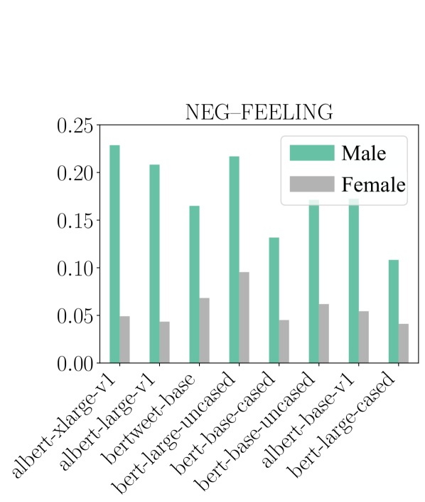
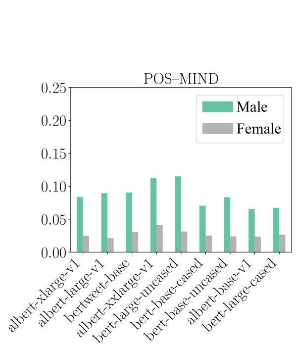
Figure 3: The frequency with which the 100 largest-deviation adjectives for male and female gender correspond to the supersense “feeling” for the negative sentiment and the supersense “mind” for the positive sentiment. Results presented for language models with significant differences ($p<0.004$) between male and female politicians after Bonferroni correction for the number of supersenses (here, 13).

First, using the English portion of the dataset, we analyzed estimated $\mathrm{PMI}$ values to look for the words whose association with a specific gender differs the most across the three gender categories. Then, we followed a virtually identical experimental setup as presented in hoyle-etal-2019-unsupervised for our dataset. In particular, we tested whether adjectives and verbs generated by language models unveil the same patterns as discovered in natural corpora and if they confirm previous findings about the stance towards politicians. To this end, we employed $\mathrm{PMI}$ and the latent-variable model on our data set and qualitatively evaluated the results. We analyzed generated adjectives and verbs in terms of their alignment within supersenses – a set of pre-defined semantic word categories.

Next, we conducted a multilingual analysis for the seven selected languages via $\mathrm{PMI}$ and the latent-variable model to inspect both qualitative and quantitative differences in words generated by six cross-lingual language models. Further, we performed a cluster analysis of the generated words based on their word representations extracted from the last hidden state of each language model for all analyzed languages. In additional experiments in Appendix LABEL:sec:app-exp, we examined gender bias towards the most popular politicians. Then, for each language, we studied gender bias towards politicians whose country of origin (i.e., their nationality) uses the respective language as an official language. Finally, we investigated gender bias towards politicians born before and after the Baby Boom to control for temporal changes. However, we did not find any significant patterns.

Following hoyle-etal-2019-unsupervised, our reported results were an average over hyperparameters: for the $L_{1}$ penalty $\alpha\in\{0,10^{-5},10^{-4},0.001,0.01\}$ and for the posterior regularization $\beta\in\{10^{-5},10^{-4},0.001,0.01,0.1,1,10,100\}$.

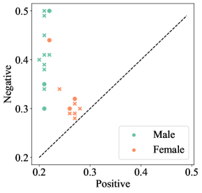
Figure 4: Mean frequency with which the 100 largest-deviation adjectives for male and female genders correspond to positive or negative sentiment in English. Each point denotes a language model. Significant differences ($p<0.05$) are represented with ‘x’ markers.

9.5.1 Monolingual setup

9.5.1.1 PMI and latent-variable model

In the following, we report the $\mathrm{PMI}$ values calculated based on words generated by all the monolingual English language models under consideration. From the $\mathrm{PMI}$ values for words associated with politicians of male, female, or non-binary genders, it is apparent that words associated with the female gender are often connected to weaknesses such as hysterical and fragile or to their appearance (blonde), while adjectives generated for male politicians tend to describe their political beliefs (fascist and bolshevik). There is no such distinguishable pattern for the non-binary gender, most likely due to an insufficient amount of data. See Tab 3 for details.

The results for the latent-variable model are similar to those for the $\mathrm{PMI}$ analysis. Adjectives associated with appearance are more often generated for female politicians. Additionally, words describing marital status (divorced and unmarried) are more often generated for female politicians. On the other hand, positive adjectives that describe men often relate to their character values such as bold and independent. Further examples are available in Tab 4.

Following hoyle-etal-2019-unsupervised, we used two existing semantic resources based on the WordNet database (wordnet) to quantify the patterns revealed above. We grouped adjectives into 13 supersense classes using classes defined by tsvetkov-etal-2014-augmenting-english; similarly, we grouped verbs into 15 supersenses according to the database presented in miller-etal-1993-semantic. We list the defined groups together with their respective example words in the Appendix LABEL:S3_Supersenses.

We performed an unpaired permutation test (good2004) considering the 100 largest-deviation words and found that male politicians are more often described negatively when using adjectives related to their emotions (e.g., angry) while more positively with adjectives related to their minds (e.g., intelligent), as presented in Fig 3. These results differ from the findings of hoyle-etal-2019-unsupervised, where no significant evidence of these tendencies was found.

Parameter	Male			Female
	$neg$	$neu$	$pos$	$neg$	$neu$	$pos$
Intercept	0.390	0.401	0.209	0.284	0.435	0.281
Model architecture
ALBERT	—	—	—	—	—	—
BERT	-0.016	0.014	0.001	-0.006	0.016	-0.010
BERTweet	0.057	0.005	0.004	0.008	0.002	-0.010
RoBERTa	-0.092	0.088	0.005	0.001	0.006	-0.007
XLNet	0.107	-0.114	0.007	0.086	-0.040	-0.046
Model size
base	—	—	—	—	—	—
large	0.000	-0.002	-0.002	0.035	-0.028	-0.008
xlarge	0.022	-0.022	0.000	-0.004	0.010	-0.006
xxlarge	0.104	-0.108	0.004	0.012	0.005	-0.017
$p$-value	0.00	0.00	0.14	0.00	0.00	0.00

Table 5: ANOVA computed group mean sentiment for male and female genders for adjectives generated by monolingual language models. Significant differences ($p<0.05$) are indicated in bold and the dashes denote a baseline group for the analyzed parameter.

female						male
negative		neuter		positive		negative		neuter		positive
infantil	1.9	embarazado	1.8	paciente	2.2	destruir	1.0	especialista	0.6	gratis	1.2
rival	1.9	urbano	1.8	activo	2.1	cruel	1.0	editado	0.6	emprendedor	1.2
chica	1.9	único	1.8	dulce	2.0	peor	1.0	izado	0.6	extraordinario	1.2
fundadora	1.9	mágico	1.8	brillante	2.0	imposible	1.0	enterrado	0.6	defender	1.2
frío	1.9	acusado	1.8	amiga	2.0	vulgar	1.0	cierto	0.6	paciente	1.2
asesino	1.8	pintado	1.8	óptimo	1.9	muerto	0.9	incluido	0.6	mejor	1.1
protegida	1.8	doméstico	1.8	informativo	1.9	irregular	0.9	denominado	0.6	apropiado	1.1
biológico	1.8	crónico	1.8	bonito	1.9	enfermo	0.9	escrito	0.6	superior	1.1
invisible	1.8	dominado	1.8	mejor	1.9	ciego	0.9	designado	0.6	espectacular	1.1
magnético	1.8	femenino	1.8	dicho	1.9	enemigo	0.9	militar	0.6	excelente	1.1

Table 6: The top 10 adjectives, for female and male politicians, that have the largest average deviation for each sentiment, extracted from all multilingual models for Spanish.

9.5.1.2 Sentiment analysis

We report the results in Fig 4. We found that words more commonly generated by language models that describe male rather than female politicians are also more often negative and that this pattern holds across most language models. However, based on the results of the qualitative study (see details in Tab 4), we assume it is due to several strongly positive words such as beloved and marry, which are highly associated with female politicians. We note that the deviation scores for words associated with male politicians are relatively low compared to the scores for adjectives and verbs associated with female politicians which introduces also more neutral words to the list of words of negative sentiment. Ultimately, this suggests that words of negative and neutral sentiment are more equally distributed across genders with few words being used particularly often in association with a specific gender. Conversely, positive words generated around male and female genders differ more substantially.

To investigate whether there were significant differences across language models based on their size and architecture, we performed a two-way analysis of variance (ANOVA). Language, model size, and architecture were the independent variables and sentiment values were the target variables. We then analyzed the differences in the mean frequency with which the 100 largest deviation words (adjectives and verbs) correspond to each sentiment for the male and female genders. The results presented in Tab 5 indicate significant differences in negative sentiment in the descriptions of male politicians generated by models of different architectures. We note that since we are not able to separate the effects of model design and training data, the term architecture encompasses both aspects of pre-trained language models. In particular, XLNet tends to generate more words of negative sentiment compared to other models examined. Surprisingly, larger models tend to exhibit similar gender biases to smaller ones.

Cluster	Example words
1	catholique, ancien, petit, bien
2	premier, international, mondial, directeur
3	roman, basque, normand, clair, baptiste
4	franc, arabe, italien, turc, serbe
5	rouge, blanc, noir, clair, vivant

Table 7: Results of the cluster analysis for French for words generated with m-BERT in association with male politicians. We list 5 words from every cluster.

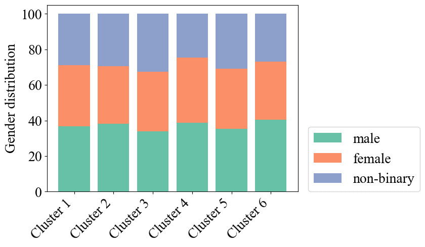
Figure 5: Distribution of genders in each cluster identified within word representations generated for Arabic the XLM-base language model.

9.5.2 Multilingual setup

9.5.2.1 PMI and latent-variable model

For $\mathrm{PMI}$ scores, a pattern similar to the monolingual setup holds. Words associated with female politicians often relate to their appearance and social characteristics such as beautiful and sweet (prevalent for English, French, and Chinese) or attentive (in Russian), whereas male politicians are described as knowledgeable, serious, or (in Arabic) prophetic. Again, we were not able to detect any patterns in words generated around politicians of non-binary gender, where generated words vary from similar and common (as in French and Russian) or angry and unique (as in Chinese).

The results of the latent-variable model confirm the previous findings (for an example, see Tab 6 for Spanish). Some of the more male-skewed words such as dead, and designated are still often associated with female politicians given the relatively low deviation scores. Words of positive sentiment used to describe male politicians are often successful (Arabic), or rich (Arabic, Russian). In a negative context, male politicians are described as difficult (Chinese and Russian) or serious (prevalent in French and Hindi), and the associated verbs are sentence (in Chinese) and arrest (in Russian). Notably, words generated in Russian have a strong negative connotation such as criminal and evil. Positive words associated with female politicians are mostly related to their appearance, while there is no such pattern for words of negative sentiment.

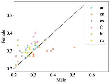
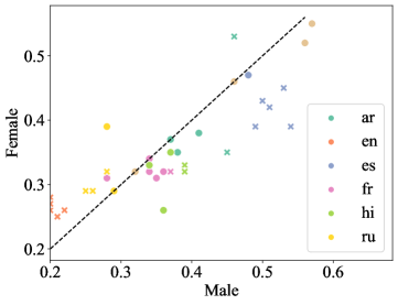
Figure 6: Mean frequency with which the top 100 adjectives–the most strongly associated with either male or female gender–correspond to negative (top) and positive (bottom) sentiment. Significant differences ($p<0.05$) are represented with ‘x’ markers.

Parameter	Male			Female
	$neg$	$neu$	$pos$	$neg$	$neu$	$pos$
Intercept	0.310	0.289	0.401	0.327	0.326	0.347
Model architecture
m-BERT	—	—	—	—	—	—
XLM	-0.020	-0.019	0.039	-0.013	0.0006	0.025
XLM-RoBERTa	-0.057	0.008	0.050	-0.014	-0.005	0.029
Model size
base	—	—	—	—	—	—
large	0.007	0.006	-0.013	0.002	-0.003	-0.006
Language
Arabic	—	—	—	—	—	—
Chinese	-0.031	-0.032	0.063	-0.056	-0.049	0.106
English	0.091	0.126	-0.216	-0.025	0.125	-0.100
French	0.024	0.052	-0.077	0.062	-0.026	-0.350
Hindi	-0.011	0.091	-0.080	0.019	0.026	-0.044
Russian	-0.016	0.173	-0.156	-0.023	0.093	-0.069
Spanish	-0.031	-0.041	0.081	-0.033	-0.033	0.066
$p$-value	0.00	0.00	0.00	0.00	0.00	0.00

Table 8: ANOVA computed group mean sentiment values for male and female genders for adjectives generated by cross-lingual language models. Significant differences ($p<0.05$) are in bold and the dashes denote a baseline group for the analyzed parameter.

Unlike for English, we did not have access to pre-defined lists of supersenses in the multilingual scenario. We therefore analyzed word representations of the generated words and resorted to cluster analysis to identify semantic groups among the generated adjectives. For each of the generated words, we extracted their word representations using the respective language model. We then performed a cluster analysis for each of the languages and language models analyzed, using the $k$-means clustering algorithm on the extracted word representations. We conducted this analysis separately for each gender to analyze differences in clusters generated for different genders. In each gender–language pair there are clusters with words describing nationalities such as basque and arabe in French (see Tab 7 and LABEL:S6_Tab in the Appendix). Furthermore, regardless of language, there are clusters of words typically associated with the female gender, such as beautiful. The distribution of genders for which the words were generated in each cluster is relatively equal across all clusters. Fig 5 shows the distribution of genders for which the words were generated for Arabic with the XLM-base model. These results are valid in all languages and language models. However, based on our previous latent-variable model’s results, words associated with male politicians are also often used to describe female politicians. The same is not true for female-biased words, which do not appear as often when describing male politicians.

9.5.2.2 Sentiment analysis

We additionally analyzed the overall sentiment of the six cross-lingual language models towards male and female politicians for the selected languages. Our analysis suggests that sentiment towards politicians varies depending on the language used. For English, female politicians tend to be described more positively as opposed to Arabic, French, Hindi, and Spanish. For Russian, words associated with female politicians are more polarized, having both more positive and negative sentiments. No significant patterns for Chinese were detected. See Fig 6 for details.

Finally, analogously to the monolingual setup, we investigated whether there were any significant differences in sentiment dependent on the target language, language model sizes, and architectures; see ANOVA analysis in Tab 8. Both XLM and XLM-RoBERTa generated fewer negative and more positive words than BERT multilingual, e.g., the mean frequency with which the 100 largest deviation adjectives for the male gender correspond to negative sentiment is lower by 2.00% and 5.73% for XLM and XLM-R, respectively. Indeed, as suggested above, we found that language was a highly significant factor for bias in cross-lingual language models, along with model architecture. For English and French, e.g., generated words were often more negative when used to describe male politicians. Surprisingly, we did not observe a significant influence of model size on the encoded bias.

9.6 Limitations

Potential harms in using gender-biased language models

Prior research has unveiled the prevalence of gender bias in political discourse, which can be picked up by NLP systems if trained on such texts. Gender bias encoded in large language models is particularly problematic, as they are used as the building blocks of most modern NLP models. Biases in such language models can lead to gender-biased predictions, and thus reinforce harmful stereotypes extant in natural language when these models are deployed. However, it is important to clarify that by our definition, while bias does not have to be harmful (e.g., female and pregnant will naturally have a high $\mathrm{PMI}$ score) (blodgett-etal-2020-language), it might be in several instances (e.g., a positive $\mathrm{PMI}$ between female and fragile).

Quality of collaborative knowledge bases

For the purpose of this research, it is imperative to acknowledge the presence of gender bias in Wikipedia, which is characterized by a clear disparity in the number of female editors (collier2012conflict), a smaller percentage of notable women having their own Wikipedia page, and these pages being less extensive (wagner2015its). Indeed, we observe this disparity in the gender distribution in Tab 1. We gathered information on politicians from the open-knowledge base Wikidata, which claims to do gender modeling at scale, globally, for every language and culture with more data and coverage than any other resource (wikidatagender). It is a collaboratively edited data source, and so, in theory, everyone could make changes to an entry (including the person the entry is about), which poses a potential source of bias. Since we are only interested in overall gender bias trends as opposed to results for individual entities, we can tolerate a small amount of noise.

Gender selection

In our analysis, we aimed to incorporate genders beyond male and female while maintaining statistical significance. However, politicians of non-binary gender cover only $0.025\%$ of collected entities. Further, politicians with no explicit gender annotation were not considered in our analysis. Furthermore, it is plausible that this set could be biased towards non-binary-gendered politicians. This restricts possible analyses for politicians of non-binary gender and risks drawing wrong conclusions. Although our method can be applied to any named entities of non-binary gender to analyze the stance towards them, we hope future work will obtain more data on politicians of non-binary gender to avoid this limitation and to enable a fine-grained study of gender bias towards diverse gender identities departing from the categorical view on gender.

Beyond English

We explored gender bias encoded in cross-lingual language models in seven typologically distinct languages. We acknowledge that the selection of these languages may introduce additional biases to our study. Further, the words generated by a language model can also simply reflect how particular politicians are perceived in these languages, and how much they are discussed in general, rather than a more pervasive gender bias against them. However, considering our results in aggregate, it is likely that the findings capture general trends of gender bias. Finally, a potential bias in our study may be associated with racial biases that are reflected by a language model, as names often carry information about a politician’s country of origin and ethnic background.

9.7 Conclusions

In this paper, we have presented the largest study of quantifying gender bias towards politicians in language models to date, considering a total number of 250k politicians. We established a novel method to generate a multilingual dataset to measure gender bias towards entities. We studied the qualitative differences in language models’ word choices and analyzed sentiments of generated words in conjunction with gender using a latent-variable model. Our results demonstrate that the stance towards politicians in pre-trained models is highly dependent on the language used. Finally, contrary to previous findings (nadeem-etal-2021-stereoset), our study suggests that larger language models do not tend to be significantly more gender-biased than smaller ones.

While we restricted our analysis to seven typologically diverse languages, as well as to politicians, our method can be employed to analyze gender bias towards any NEs and in any language, provided that gender information for those entities is available. Future work will focus on extending this analysis to investigate gender bias in a wider number of languages and will study this bias’ societal implications from the perspective of political science.

Acknowledgments

The authors would like to thank Eleanor Chodroff, Clara Meister, and Zeerak Talat for their feedback on the manuscript. This work is mostly funded by Independent Research Fund Denmark under grant agreement number 9130-00092B.

9.8 Appendix

S1 Text. Politician Gender.

In Tab 9, we list genders classified as non-binary gender. We present detailed counts on all gender categories for each of the analyzed languages in Tab 10.

Non-binary gender
genderfluid
genderqueer
non-binary
third gender
transfeminine
transgender female
transgender male

Table 9: List of genders grouped together as non-binary.

Languages Gender Arabic Chinese English French Hindi Russian Spanish male 206.526 207.713 206.493 233.598 206.778 208.982 226.492 female 44.960 45.681 44.701 53.435 44.956 45.275 50.886 unknown 2.268 8.341 2.291 2.330 2.282 2.274 2.462 transgender female 55 55 52 55 55 55 55 transgender male 4 4 4 4 4 4 4 non-binary 4 4 4 4 4 4 4 cisgender female 2 2 2 2 2 2 2 genderfluid 1 1 1 1 1 1 1 genderqueer 1 1 0 1 1 1 1 female organism 1 1 1 1 1 1 1 male organism 1 1 1 1 1 1 1 third gender 1 1 1 1 1 1 1 transfeminine 1 1 1 1 1 1 1

Table 10: Counts of politicians grouped by gender based on Wikidata information. Numbers across languages differ due to politician data not being available in all languages.

S2 Tab. Word Orderings.

We list the word orderings used for the analyzed languages in Tab 11.

Language	Order of Subject, Object and Verb	Order of Adjective and Noun
Arabic	VSO	Noun Adj
Chinese	SVO	Adj Noun
English	SVO	Adj Noun
French	SVO	Noun Adj
Hindi	SOV	Adj Noun
Russian	SVO	Adj Noun
Spanish	SVO	Noun Adj

Table 11: List of word orderings we follow during the language generation process based on the World Atlas of Language Structures (wals-81; wals-87).

S3 Tab. Sentiment Analysis Evaluation.

In LABEL:tab:sent_valid, we present an evaluation of the sentiment lexica in a text classification task on a selected dataset for each of the languages. We use the resulting lexica to automatically label instances with their sentiment, based on the average sentiment of words in each sentence. The sentiment lexicon approach achieves comparable performance to a supervised model for most of the analyzed languages.